Optimal and Robust Controller Synthesis - arxiv.org · Optimal and Robust Controller Synthesis 3...

Optimal and Robust Controller Synthesis?

Using Energy Timed Automata with Uncertainty

Giovanni Bacci1, Patricia Bouyer2, Uli Fahrenberg3, Kim G. Larsen1,Nicolas Markey4, and Pierre-Alain Reynier5

1 Department of Computer Science, Aalborg University, Denmark2 LSV, CNRS & ENS Cachan, Universite Paris-Saclay, Cachan, France

3 Ecole Polytechnique, Palaiseau, France4 Univ. Rennes, IRISA, CNRS & INRIA, Rennes, France

5 Aix-Marseille Univ, LIF, CNRS, Marseille, France

Abstract. In this paper, we propose a novel framework for the synthesisof robust and optimal energy-aware controllers. The framework is based onenergy timed automata, allowing for easy expression of timing constraintsand variable energy rates. We prove decidability of the energy-constrainedinfinite-run problem in settings with both certainty and uncertainty of theenergy rates. We also consider the optimization problem of identifying theminimal upper bound that will permit existence of energy-constrainedinfinite runs. Our algorithms are based on quantifier elimination forlinear real arithmetic. Using Mathematica and Mjollnir, we illustrate ourframework through a real industrial example of a hydraulic oil pump.Compared with previous approaches our method is completely automatedand provides improved results.

1 Introduction

Design of controllers for embedded systems is a difficult engineering task. Con-trollers must ensure a variety of safety properties as well as optimality withrespect to given performance properties. Also, for several systems, e.g. [8,27,25],the properties involve non-functional aspects such as time and energy.

We provide a novel framework for automatic synthesis of safe and optimal con-trollers for resource-aware systems based on energy timed automata. Synthesis ofcontrollers is obtained by solving time- and energy-constrained infinite run prob-lems. Energy timed automata [12] extend timed automata [2] with a continuousenergy variable that evolves with varying rates and discrete updates during the be-haviour of the model. Closing an open problem from [12], we prove decidability ofthe infinite run problem in settings, where rates and updates may be both positiveand negative and possibly subject to uncertainty. Additionally, the accumulatedenergy may be subject to lower and upper bounds reflecting constraints on ca-pacity. Also we consider the optimization problems of identifying minimal upperbounds that will permit the existence of infinite energy-constrained runs. Our deci-sion and optimization algorithms for the energy-constrained infinite run problems

? Work supported by ERC projects Lasso and EQualIS.

arX

iv:1

805.

0084

7v2

[cs

.FL

] 3

May

201

8

2 G. Bacci, P. Bouyer, U. Fahrenberg, K.G. Larsen, N. Markey, P.A. Reynier

Pump

Machine

2.2 l/s

Vmax

Vmin

Accumulator

(a) System Components

Automatic Synthesis of Robust and Optimal Controllers – An Industrial Case Study 93

i1 i2 i3 i4 i5

i6i7i8i9

[t ≤ 2][t ≤ 4] [t ≤ 8] [t ≤ 10] [t ≤ 12]

[t ≤ 14][t ≤ 16][t ≤ 18][t ≤ 20]

mr := 0t := 0

t = 2mr :=1.2

t = 4mr :=0

t = 8mr :=1.2

t = 10mr :=2.5

t = 12mr :=0

t = 14mr :=1.7

t = 16mr :=0.5

t = 18mr :=0

t = 20t :=0

(a) The Machine

dvdt ∈ [pr − m+

r (ϵ); pr − m−r (ϵ)]

dVaccdt = v

[true]

v := 10.0Vacc := 0

(b) The Accumulator

Off On

[true] [true]

z := 2pr := 0

z ≥ 2, switch on!pr := 2.2, z := 0

z ≥ 2, switch off!pr := 0, z := 0

(c) The Pump

0 2 4 6 8 10 12 14 16 18 200.00.20.40.60.81.01.21.41.61.82.02.22.42.62.83.0

Time (second)

1.2 1.2

2.5

1.7

0.5

Mac

hine

Rat

e (l

itre/

seco

nd)

(d) Cycle of the Machine

Fig. 2. Hybrid Automaton Model of the System

– (R2): a large amount of oil in the accumulator implies a high pressure of gas in theaccumulator. This requires more energy from the pump to fill in the accumulatorand also speeds up the wear of the machine. This is why the level of oil should bekept minimal during operation, in the sense that

! t=T

t=0v(t)dt, that is Vacc(T ), is

minimal for a given operation period T .

While (R1) is a safety requirement and so must never be violated by any controller, (R2)is an optimality requirement and will be used to compare different controllers.

Note that as the power of the pump is not always larger than the demand of the ma-chine during one period of consumption (see Fig. 2(d) between 10and 12), some extraamount of oil must be present in the accumulator before that period of consumption toensure that the minimal amount of oil constraint (requirement R1) is not violated1.

Additional Requirements on the Controller. When designing a controller, we must de-cide what are the possible actions that the controller can take. Here are some consid-erations about that. First, as the consumptions are subject to noise, it is necessary toallow the controller to check periodically the level of oil in the accumulator (as it is notpredictable in the long run). Second, as the consumption of the machine has a cyclicbehavior, the controller should use this information to optimize the level of oil. So, it isnatural to allow the controller to take control decisions at predefined instants during thecycle. Finally, we want a robust solution in the sense that if the controller has to turnon (or off) the pump at time t, it can do it a little before or after, that is at time t ± ∆

1 It might be too late to switch the pump on when the volume reaches Vmin.

(b) Cycle of the Machine

Fig. 1: Overview of the HYDAC system

are based on reductions to quantifier elimination (QE) for linear real arithmetic,for which we combine Mathematica [28] and Mjollnir [24] into a tool chain.

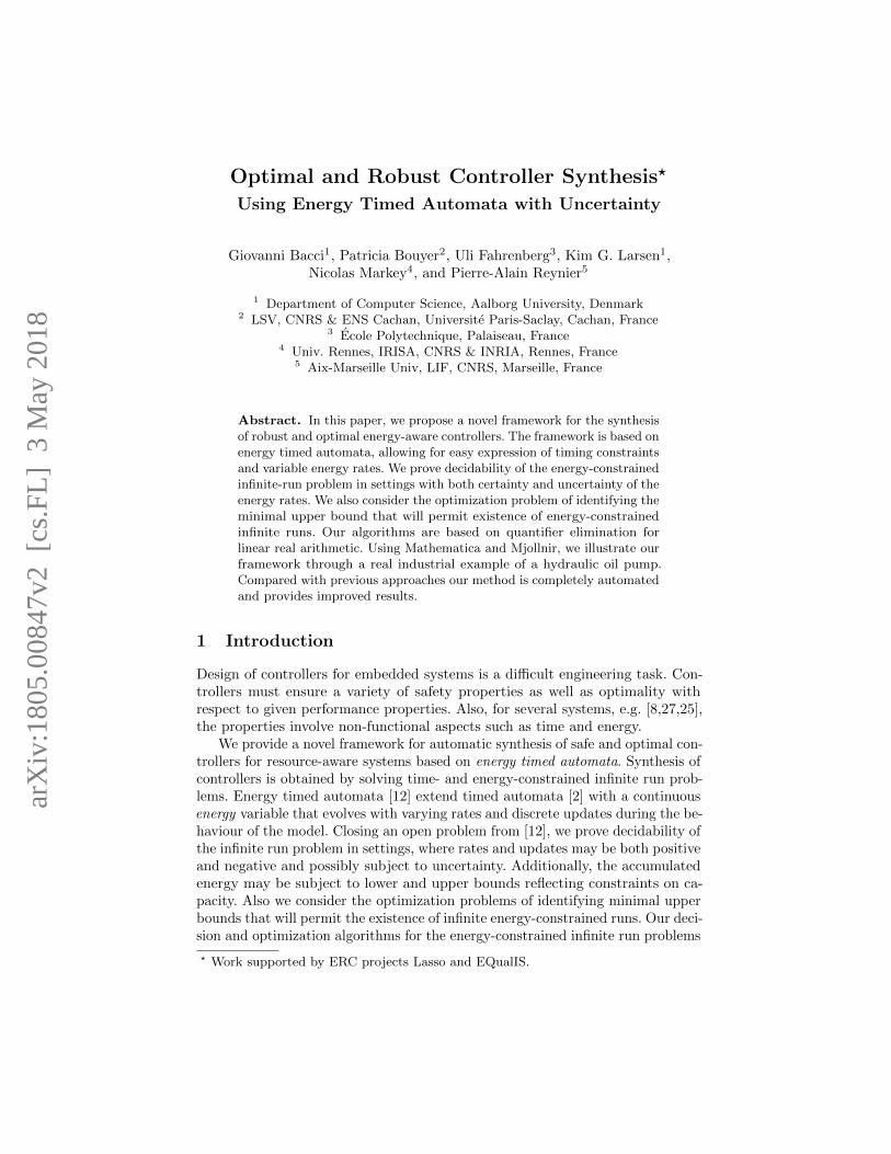
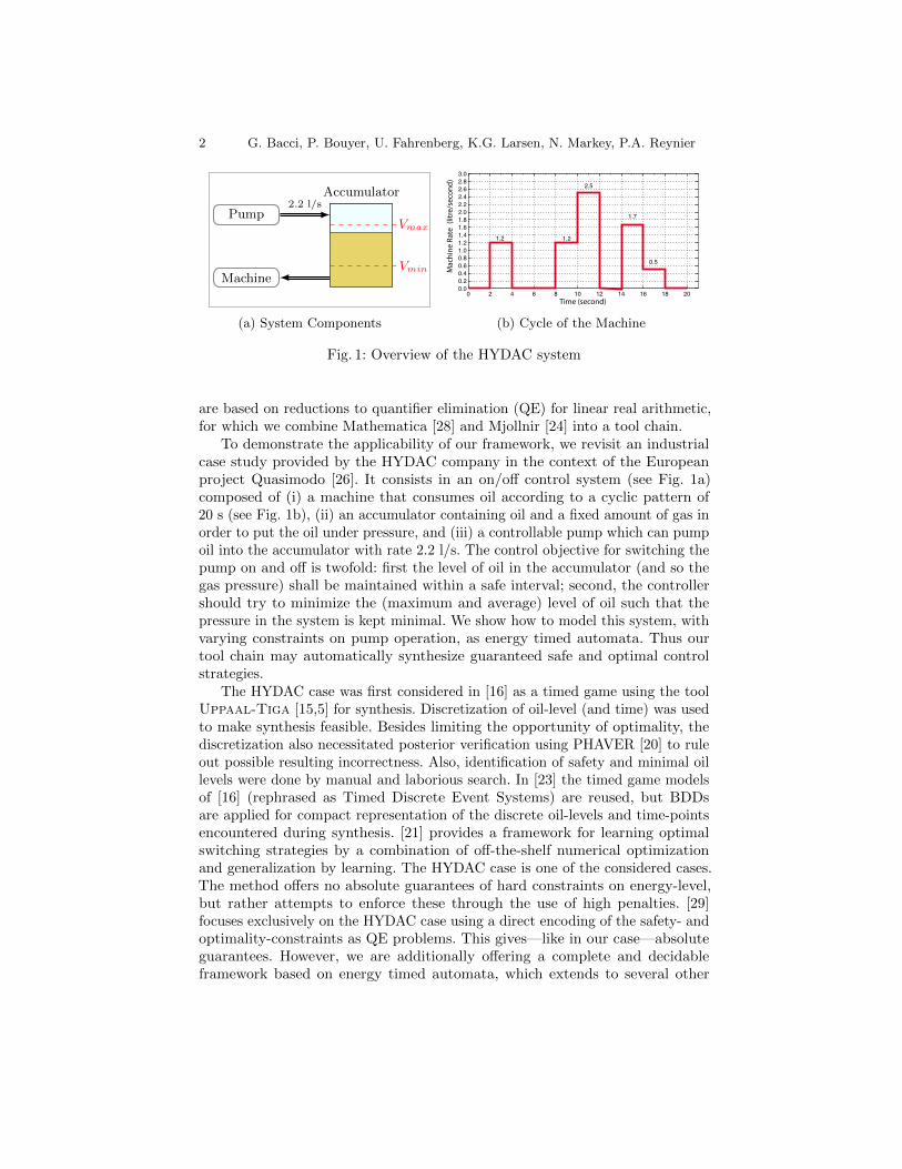
To demonstrate the applicability of our framework, we revisit an industrialcase study provided by the HYDAC company in the context of the Europeanproject Quasimodo [26]. It consists in an on/off control system (see Fig. 1a)composed of (i) a machine that consumes oil according to a cyclic pattern of20 s (see Fig. 1b), (ii) an accumulator containing oil and a fixed amount of gas inorder to put the oil under pressure, and (iii) a controllable pump which can pumpoil into the accumulator with rate 2.2 l/s. The control objective for switching thepump on and off is twofold: first the level of oil in the accumulator (and so thegas pressure) shall be maintained within a safe interval; second, the controllershould try to minimize the (maximum and average) level of oil such that thepressure in the system is kept minimal. We show how to model this system, withvarying constraints on pump operation, as energy timed automata. Thus ourtool chain may automatically synthesize guaranteed safe and optimal controlstrategies.

The HYDAC case was first considered in [16] as a timed game using the toolUppaal-Tiga [15,5] for synthesis. Discretization of oil-level (and time) was usedto make synthesis feasible. Besides limiting the opportunity of optimality, thediscretization also necessitated posterior verification using PHAVER [20] to ruleout possible resulting incorrectness. Also, identification of safety and minimal oillevels were done by manual and laborious search. In [23] the timed game modelsof [16] (rephrased as Timed Discrete Event Systems) are reused, but BDDsare applied for compact representation of the discrete oil-levels and time-pointsencountered during synthesis. [21] provides a framework for learning optimalswitching strategies by a combination of off-the-shelf numerical optimizationand generalization by learning. The HYDAC case is one of the considered cases.The method offers no absolute guarantees of hard constraints on energy-level,but rather attempts to enforce these through the use of high penalties. [29]focuses exclusively on the HYDAC case using a direct encoding of the safety- andoptimality-constraints as QE problems. This gives—like in our case—absoluteguarantees. However, we are additionally offering a complete and decidableframework based on energy timed automata, which extends to several other

Optimal and Robust Controller Synthesis 3

systems. Moreover, the controllers we obtain perform significantly better thanthose of [16] and [29] (respectively up to 22% and 16% better) and are obtainedautomatically by our tool chain combining Mjollnir and Mathematica. Thiscombination permits quantifier elimination and formula simplification to bedone in a compositional manner, resulting in performance surpassing each toolindividually. We believe that this shows that our framework has a level of maturitythat meets the complexity of several relevant industrial control problems.

Our work is related to controllability of (constrained) piecewise affine (PWA) [7]and hybrid systems [1]. In particular, the energy-constrained infinite-run problemis related to the so called stability problem for PWAs. Blondel and Tsitsiklis [10]have shown that verifying stability of autonomous piecewise-linear (PWL) sys-tems is NP-hard, even in the simple case of two-component subsystems; severalglobal properties (e.g. global convergence, asymptotic stability and mortality) ofPWA systems have been shown undecidable in [9].

2 Energy Timed Automata

Definitions. Given a finite set X of clocks, the set of closed clock constraintsover X, denoted C(X), is the set of formulas built using g ::= x ∼ n | g∧g, wherex ranges over X, ∼ ranges over {≤,≥} and n ranges over Q≥0. That a clockvaluation v : X → R≥0 satisfies a clock constraint g, denoted v |= g, is defined inthe natural way. For a clock valuation v, a real t ∈ R≥0, and a subset R ⊆ X,we write v + t for the valuation mapping each clock x ∈ X to v(x) + t, andv[R → 0] for the valuation mapping clocks in R to zero and clocks not in Rto their value in v. Finally we write 0X (or simply 0) for the clock valuationassigning 0 to every x ∈ X.

For E ⊆ R, we let I(E) be the set of closed intervals of R with boundsin E ∩Q. Notice that any interval in I(E) is bounded, for any E ⊆ R.

Definition 1. An energy timed automaton ( ETA for short; a.k.a. priced orweighted timed automaton [3,6]) is a tuple A = (S, S0, X, I, r, T ) where S is afinite set of states, S0 ⊆ S is the set of initial states, X is a finite set of clocks,I : S → C(X) assigns invariants to states, r : S → Q assigns rates to states, andT ⊆ S × C(X)×Q× 2X × S is a finite set of transitions.

An energy timed path ( ETP, a.k.a. linear energy timed automaton) is anenergy timed automaton for which S can be written as {si | 0 ≤ i ≤ n} in such away that S0 = {s0}, and T = {(si, gi, ui, zi, si+1) | 0 ≤ i < n}. We additionallyrequire that all clocks are reset on the last transition, i.e., zn−1 = X.

Let A = (S, S0, X, I, r, T ) be an ETA. A configuration of A is a triple(`, v, w) ∈ S × (R≥0)X × R, where v is a clock valuation, and w is the en-ergy level. Let τ = (ti)0≤i<n be a finite sequence of transitions, with ti =(si, gi, ui, zi, si+1) for every i. A finite run in A on τ is a sequence of configura-tions ρ = (`j , vj , wj)0≤j≤2n such that there exists a sequence of delays (di)0≤i<nfor which the following requirements hold:


s0

y ≤ 1

r : +2

P: s1

y ≤ 1

r : +4

s2y ≥ 1

4 u : −3

y := 0

x = 1

x := 0, y := 0

u : 0

w

t10

s0

s0

s1

s1s2

ρ

Fig. 2: An energy timed path P, and a run ρ of P with initial energy level 3.

– for all 0 ≤ j < n, `2j = `2j+1 = sj , and `2n = sn;– for all 0 ≤ j < n, v2j+1 = v2j + dj and v2j+2 = v2j+1[zj → 0];– for all 0 ≤ j < n, v2j |= I(sj) and v2j+1 |= I(sj) ∧ gj ;– for all 0 ≤ j < n, w2j+1 = w2j + dj · r(sj) and w2j+2 = w2j+1 + uj .

We will by extension speak of runs read on ETPs (those runs will then end withclock valuation 0). The notion of infinite run is defined similarly. Given E ∈ I(Q),such a run is said to satisfy energy constraint E if wj ∈ E for all j.

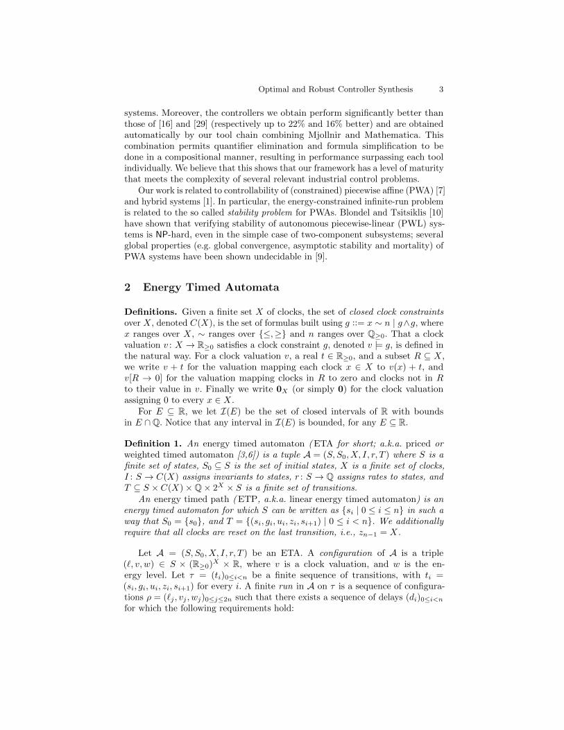
Example 1. Fig. 2 displays an example of an ETP P and one of its runs ρ. Sinceno time will be spent in s2, we did not indicate the invariant and rate of thatstate. The sequence ρ is a run of P. Spending 0.6 time units in s0, the value ofclock x reaches 0.6, and the energy level grows to 3 + 0.6× 2 = 4.2; it equals4.2− 3 = 1.2 when entering s1. Then ρ satisfies energy constraint [0; 5]. /

Definition 2. A segmented energy timed automaton ( SETA for short) is atuple A = (S, T, P ) where (S, T ) is a finite graph (whose states and transitionsare called macro-states and macro-transitions), S0 is a set of initial macro-states,and P associates with each macro-transition t = (s, s′) of A an ETP with initialstate s and final state s′. We require that for any two different transitions t and t′

of A, the state spaces of P (t) and P (t′) are disjoint and contain no macro-states,except (for both conditions) for their first and last states.

A SETA is flat if the underlying graph (S, T ) is (i.e., for any s ∈ S, thereis at most one non-empty path in the graph (S, T ) from s to itself [17,14]). It iscalled depth-1 whenever the graph (S, T ) is tree-like, with only loops at leaves.

A (finite or infinite) execution of a SETA is a (finite or infinite) sequence ofruns ρ = (ρi)i such that for all i, writing ρi = (ìj , v

ij , w

ij)0≤j≤2ni

, it holds:

– ì0 and ì2niare macro-states of A, and ρi is a run of the ETP P (ì0, `

i2ni

);

– ì+10 = ì2ni

and wi+10 = wi2ni

.

Hence a run in a SETA should be seen as the concatenation of paths ρi betweenmacro-states. Notice also that each ρi starts and ends with all clock values zero,since all clocks are reset at the end of each ETP, when a main state is entered. Fi-nally, given an interval E ∈ I(Q), an execution (ρi)i satisfies energy constraint Ewhenever all individual runs ρi do.


s0(S, T ) : s2

P0,2 =

P2,2 =

s0

r:0

s2s1

r:−1

y:=0

u:+1

x:=0y:=0

x≥1

s2

r:+2

s3

r:+4

s2y≥0.25 u:−3

y:=0

x=1

x:=0y:=0

w

t1 2 30

s0s0

s1 s1s2

ρ1

s2

s3

s3s2

ρ2

s2

s3

s3s2

ρ3

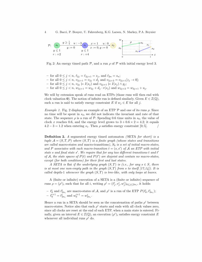
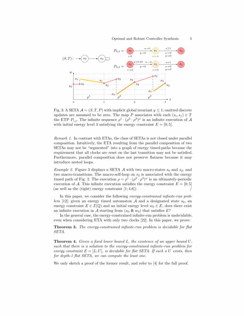
Fig. 3: A SETAA = (S, T, P ) with implicit global invariant y ≤ 1; omitted discreteupdates are assumed to be zero. The map P associates with each (si, sj) ∈ Tthe ETP Pi,j . The infinite sequence ρ1 · (ρ2 · ρ3)ω is an infinite execution of Awith initial energy level 3 satisfying the energy constraint E = [0; 5].

Remark 1. In contrast with ETAs, the class of SETAs is not closed under parallelcomposition. Intuitively, the ETA resulting from the parallel composition of twoSETAs may not be “segmented” into a graph of energy timed-paths because therequirement that all clocks are reset on the last transition may not be satisfied.Furthermore, parallel composition does not preserve flatness because it mayintroduce nested loops.

Example 2. Figure 3 displays a SETA A with two macro-states s0 and s2, andtwo macro-transitions. The macro-self-loop on s2 is associated with the energytimed path of Fig. 2. The execution ρ = ρ1 · (ρ2 · ρ3)ω is an ultimately-periodicexecution of A. This infinite execution satisfies the energy constraint E = [0; 5](as well as the (tight) energy constraint [1; 4.6]). /

In this paper, we consider the following energy-constrained infinite-run prob-lem [12]: given an energy timed automaton A and a designated state s0, anenergy constraint E ∈ I(Q) and an initial energy level w0 ∈ E, does there existan infinite execution in A starting from (s0,0, w0) that satisfies E?

In the general case, the energy-constrained infinite-run problem is undecidable,even when considering ETA with only two clocks [22]. In this paper, we prove:

Theorem 3. The energy-constrained infinite-run problem is decidable for flatSETA.

Theorem 4. Given a fixed lower bound L, the existence of an upper bound U ,such that there is a solution to the energy-constrained infinite-run problem forenergy constraint E = [L;U ], is decidable for flat SETA. If such a U exists, thenfor depth-1 flat SETA, we can compute the least one.

We only sketch a proof of the former result, and refer to [4] for the full proof.


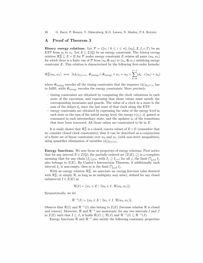
Binary energy relations. Let P = ({si | 0 ≤ i ≤ n}, {s0}, X, I, r, T ) be anETP from s0 to sn. Let E ⊆ I(Q) be an energy constraint. The binary energyrelation REP ⊆ E ×E for P under energy constraint E relates all pairs (w0, w1)for which there is a finite run of P from (s0,0, w0) to (sn,0, w1) satisfying energyconstraint E. This relation is characterized by the following first-order formula:

REP(w0, w1) ⇐⇒ ∃(di)0≤i<n. Φtiming ∧ Φenergy ∧ w1 = w0 +

n−1∑

k=0

(dk · r(sk) + uk)

where Φtiming encodes all the timing constraints that the sequence (di)0≤i<nhas to fulfill (derived from guards and invariants, by expressing the values ofthe clocks in terms of (di)0≤i<n), while Φenergy encodes the energy constraints(in each state, the accumulated energy must be in E).

w0

w1

00

1

1

2

2

3

3

4

4

5

5

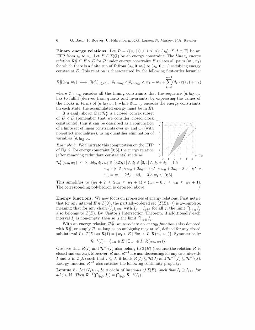
It is easily shown that REP is a closed, convex subsetof E × E (remember that we consider closed clockconstraints); thus it can be described as a conjunctionof a finite set of linear constraints over w0 and w1 (withnon-strict inequalities), using quantifier elimination ofvariables (di)0≤i<n.

Example 3. We illustrate this computation on the ETPof Fig. 2. For energy constraint [0; 5], the energy relation(after removing redundant constraints) reads as

REP(w0, w1) ⇐⇒ ∃d0, d1. d0 ∈ [0.25; 1] ∧ d1 ∈ [0; 1] ∧ d0 + d1 = 1 ∧w0 ∈ [0; 5] ∧ w0 + 2d0 ∈ [0; 5] ∧ w0 + 2d0 − 3 ∈ [0; 5] ∧w1 = w0 + 2d0 + 4d1 − 3 ∧ w1 ∈ [0; 5].

This simplifies to (w1 + 2 ≤ 2w0 ≤ w1 + 4) ∧ (w1 − 0.5 ≤ w0 ≤ w1 + 1).The corresponding polyhedron is depicted above. /

Energy functions. We now focus on properties of energy relations. First noticethat for any interval E ∈ I(Q), the partially-ordered set (I(E),⊇) is ω-complete,meaning that for any chain (Ij)j∈N, with Ij ⊇ Ij+1 for all j, the limit

⋂j∈N Ij

also belongs to I(E). By Cantor’s Intersection Theorem, if additionally eachinterval Ij is non-empty, then so is the limit

⋂j∈N Ij .

With an energy relation REP , we associate an energy function (also denotedwith REP , or simply R, as long as no ambiguity may arise), defined for any closedsub-interval I ∈ I(E) as R(I) = {w1 ∈ E | ∃w0 ∈ I. R(w0, w1)}. Symmetrically:

R−1(I) = {w0 ∈ E | ∃w1 ∈ I. R(w0, w1)}.Observe that R(I) and R−1(I) also belong to I(E) (because the relation R isclosed and convex). Moreover,R andR−1 are non-decreasing: for any two intervalsI and J in I(E) such that I ⊆ J , it holds R(I) ⊆ R(J) and R−1(I) ⊆ R−1(J).Energy function R−1 also satisfies the following continuity property:

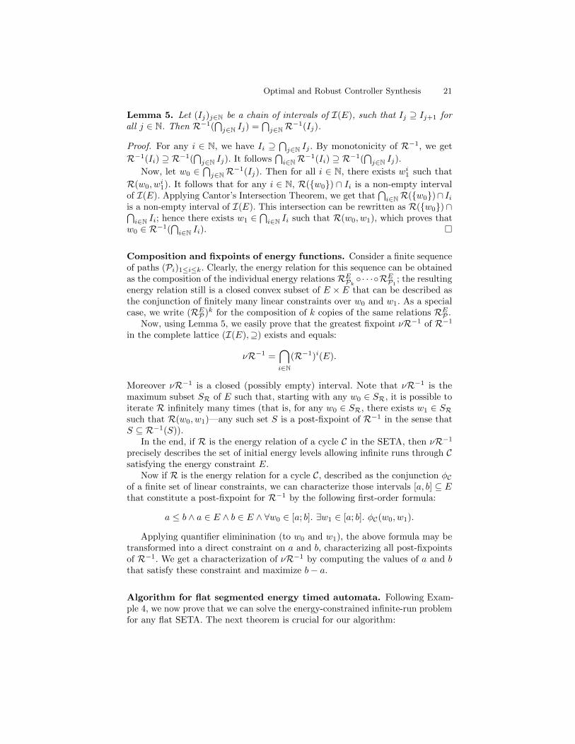
Lemma 5. Let (Ij)j∈N be a chain of intervals of I(E), such that Ij ⊇ Ij+1 forall j ∈ N. Then R−1(

⋂j∈N Ij) =

⋂j∈NR−1(Ij).


Composition and fixpoints of energy functions. Consider a finite sequenceof paths (Pi)1≤i≤k. Clearly, the energy relation for this sequence can be obtainedas the composition of the individual energy relations REPk

◦· · ·◦REP1; the resulting

energy relation still is a closed convex subset of E ×E that can be described asthe conjunction of finitely many linear constraints over w0 and w1. As a specialcase, we write (REP)k for the composition of k copies of the same relations REP .

Now, using Lemma 5, we easily prove that the greatest fixpoint νR−1 of R−1

in the complete lattice (I(E),⊇) exists and equals:

νR−1 =⋂

i∈N(R−1)i(E).

Moreover νR−1 is a closed (possibly empty) interval. Note that νR−1 is themaximum subset SR of E such that, starting with any w0 ∈ SR, it is possible toiterate R infinitely many times (that is, for any w0 ∈ SR, there exists w1 ∈ SRsuch that R(w0, w1)—any such set S is a post-fixpoint of R−1, i.e. S ⊆ R−1(S)).

If R is the energy relation of a cycle C in the flat SETA, then νR−1 preciselydescribes the set of initial energy levels allowing infinite runs through C satisfyingthe energy constraint E. If R is described as the conjunction φC of a finite setof linear constraints, then we can characterize those intervals [a, b] ⊆ E thatconstitute a post-fixpoint for R−1 by the following first-order formula:

a ≤ b ∧ a ∈ E ∧ b ∈ E ∧ ∀w0 ∈ [a; b]. ∃w1 ∈ [a; b]. φC(w0, w1). (1)

Applying quantifier elimination (to w0 and w1), the above formula may betransformed into a direct constraint on a and b, characterizing all post-fixpointsof R−1. We get a characterization of νR−1 by computing the values of a and bthat satisfy these constraint and maximize b− a.

Example 4. We again consider the flat SETA of Fig. 3, and consider the energyconstraint E = [0; 5]. We first focus on the cycle C on the macro-state s2: using theenergy relation computed in Example 3, our first-order formula for the fixpointthen reads as follows:

0 ≤ a ≤ b ≤ 5 ∧ ∀w0 ∈ [a; b]. ∃w1 ∈ [a; b].((w1 + 2 ≤ 2w0 ≤ w1 + 4) ∧ (w1 − 0.5 ≤ w0 ≤ w1 + 1)

).

Applying quantifier elimination, we end up with 2 ≤ a ≤ b ≤ 4. The maximalfixpoint then is [2; 4]. Similarly, for the path P from s0 to s2:

REP(w0, w1) ⇐⇒ ∃d0, d1. 0 ≤ d0 ≤ 1 ∧ 0 ≤ d1 ≤ 1 ∧ d0 + d1 ≥ 1 ∧0 ≤ w0 ≤ 5 ∧ 0 ≤ w0 + 1 ≤ 5 ∧ w1 = w1 + 1− d1 ∧ 0 ≤ w1 ≤ 5

which reduces to 0 ≤ w0 ≤ 4 ∧ w0 ≤ w1 ≤ w0 + 1. Finally, the initial energylevels w0 for which there is an infinite-run in the whole SETA are characterizedby ∃w1. (0 ≤ w0 ≤ 4 ∧ w0 ≤ w1 ≤ w0 + 1) ∧ (2 ≤ w1 ≤ 4), which reduces to1 ≤ w0 ≤ 4. /


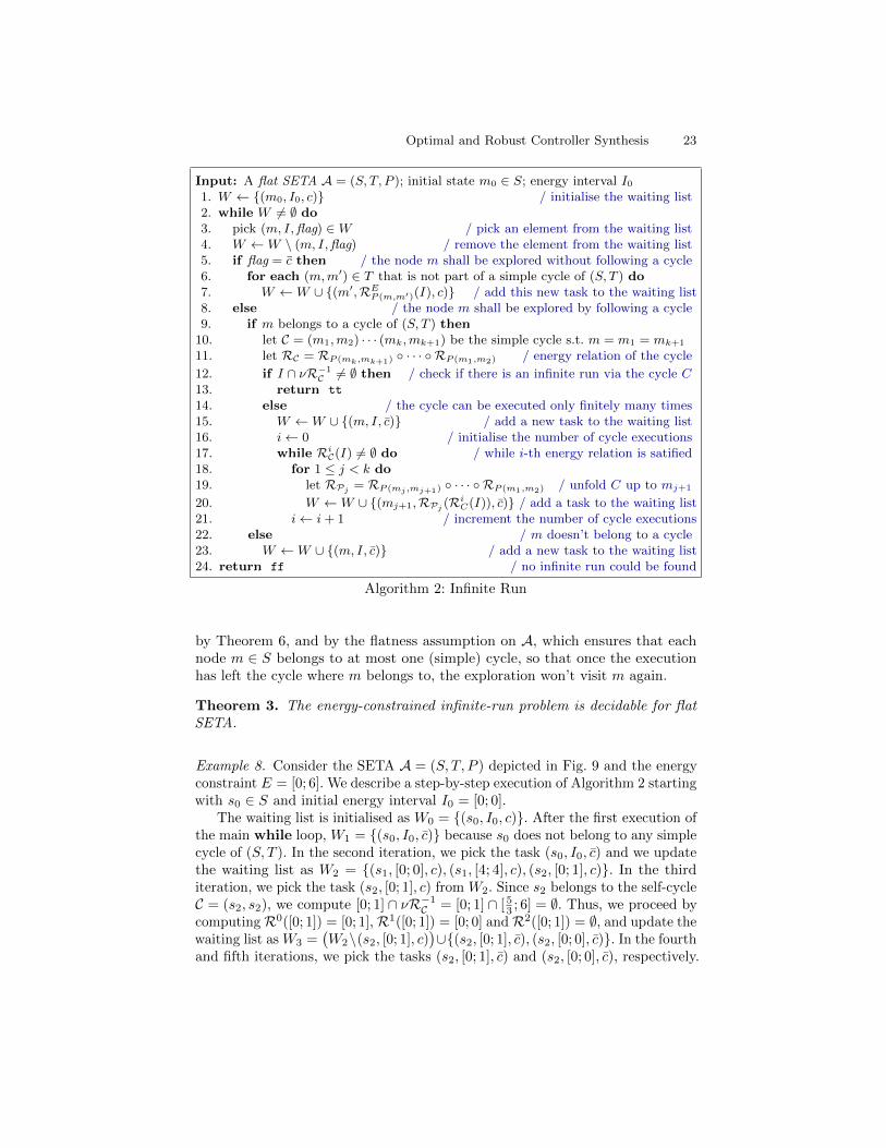
Input: A flat SETA A = (S, T, P ); initial state m0 ∈ S; energy interval I01. W ← {(m0, I0, c)} / initialize the waiting list2. while W 6= ∅ do3. pick (m, I,flag) ∈W / pick an element from the waiting list4. W ←W \ (m, I,flag) / remove the element from the waiting list5. if flag = c then / the node m shall be explored without following a cycle6. for each (m,m′) ∈ T that is not part of a simple cycle of (S, T ) do7. W ←W ∪ {(m′,RE

P (m,m′)(I), c)} / add this new task to the waiting list8. else / the node m shall be explored by following a cycle9. if m belongs to a cycle of (S, T ) then

10. let C = (m1,m2) · · · (mk,mk+1) be the simple cycle s.t. m = m1 = mk+1

11. let RC = RP (mk,mk+1) ◦ · · · ◦ RP (m1,m2) / energy relation of the cycle

12. if I ∩ νR−1C 6= ∅ then / check if there is an infinite run via the cycle C

13. return tt

14. else / the cycle can be executed only finitely many times15. W ←W ∪ {(m, I, c)} / add a new task to the waiting list16. i← 0 / initialize the number of cycle executions17. while Ri

C(I) 6= ∅ do / while i-th energy relation is satisfied18. for 1 ≤ j < k do19. let RPj = RP (mj ,mj+1) ◦ · · · ◦ RP (m1,m2) / unfold C up to mj+1

20. W ←W ∪ {(mj+1,RPj (RiC(I)), c)}/ add a task to the waiting list

21. i← i+ 1 / increment the number of cycle executions22. else / m doesn’t belong to a cycle23. W ←W ∪ {(m, I, c)} / add a new task to the waiting list24. return ff / no infinite run could be found

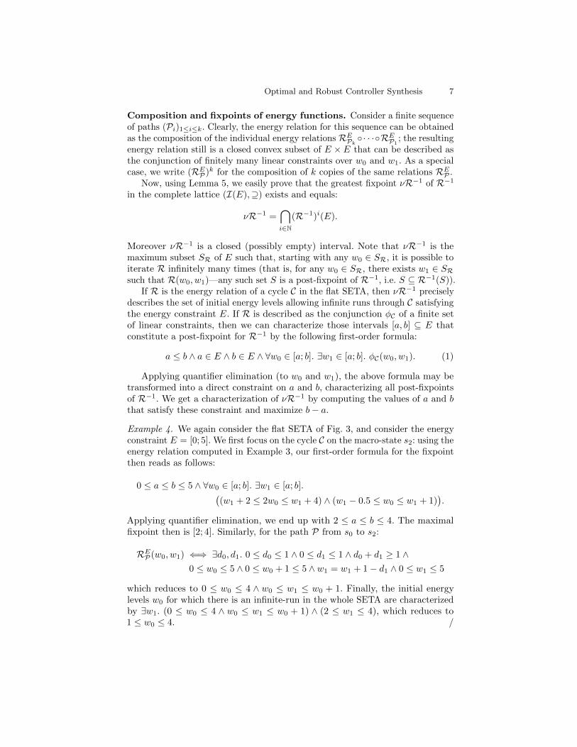
Algorithm 1: Existence of energy-constrained infinite runs in flat SETA

Algorithm for flat segmented energy timed automata. Following Exam-ple 4, we now prove that we can solve the energy-constrained infinite-run problemfor any flat SETA. The next theorem is crucial for our algorithm:

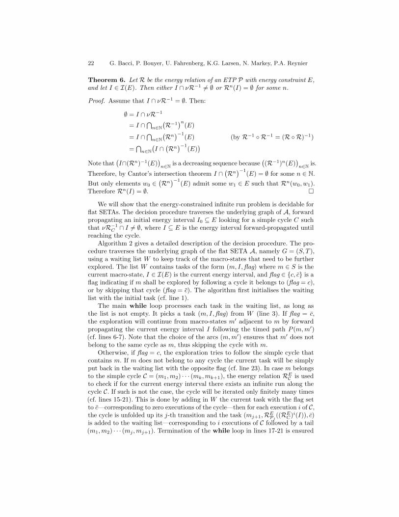
Theorem 6. Let R be the energy relation of an ETP P with energy constraint E,and let I ∈ I(E). Then either I ∩ νR−1 6= ∅ or Rn(I) = ∅ for some n.

It follows that the energy-constrained infinite-run problem is decidable forflat SETAs. The decision procedure traverses the underlying graph of A, forwardpropagating an initial energy interval I0 ⊆ E looking for a simple cycle C suchthat νR−1

C ∩ I 6= ∅, where I ⊆ E is the energy interval forward-propagateduntil reaching the cycle. Algorithm 1 gives a detailed description of the decisionprocedure. It traverses the underlying graph (S, T ) of the flat SETA A, using awaiting list W to keep track of the macro-states that need to be further explored.The list W contains tasks of the form (m, I,flag) where m ∈ S is the currentmacro-state, I ∈ I(E) is the current energy interval, and flag ∈ {c, c} is a flagindicating if m shall be explored by following a cycle it belongs to (flag = c), orproceed by exiting that cycle (flag = c). Theorem 6 ensures termination of thewhile loop of lines 17-21, whereas flatness ensures the correctness of Algorithm 1.


It is worth noting that the flatness assumption for the SETA A implies thatthe graph (S, T ) has finitely many cycles (each macro-state belongs to at mostone simple cycle of (S, T ), therefore the number of cycles is bounded by thenumber of macro-states). As a consequence, Algorithm 1 performs in the worstcase an exhaustive search of all cycles in A. The technique does not triviallyextend to SETAs with nested cycles, because they may have infinitely manycycles.

3 Energy Timed Automata with Uncertainties

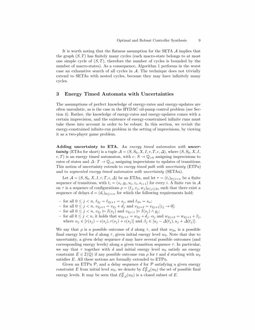
The assumptions of perfect knowledge of energy-rates and energy-updates areoften unrealistic, as is the case in the HYDAC oil-pump control problem (see Sec-tion 4). Rather, the knowledge of energy-rates and energy-updates comes with acertain imprecision, and the existence of energy-constrained infinite runs musttake these into account in order to be robust. In this section, we revisit theenergy-constrained infinite-run problem in the setting of imprecisions, by viewingit as a two-player game problem.

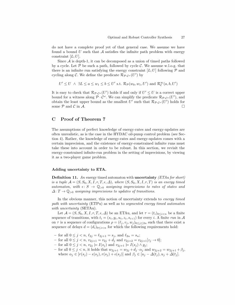
Adding uncertainty to ETA. An energy timed automaton with uncer-tainty (ETAu for short) is a tuple A = (S, S0, X, I, r, T, ε,∆), where (S, S0, X, I,r, T ) is an energy timed automaton, with ε : S → Q>0 assigning imprecisions torates of states and ∆ : T → Q>0 assigning imprecisions to updates of transitions.This notion of uncertainty extends to energy timed path with uncertainty (ETPu)and to segmented energy timed automaton with uncertainty (SETAu).

Let A = (S, S0, X, I, r, T, ε,∆) be an ETAu, and let τ = (ti)0≤i<n be a finitesequence of transitions, with ti = (si, gi, ui, zi, si+1) for every i. A finite run in Aon τ is a sequence of configurations ρ = (`j , vj , wj)0≤j≤2n such that there exist asequence of delays d = (di)0≤i<n for which the following requirements hold:

– for all 0 ≤ j < n, `2j = `2j+1 = sj , and `2n = sn;– for all 0 ≤ j < n, v2j+1 = v2j + dj and v2j+2 = v2j+1[zj → 0];– for all 0 ≤ j < n, v2j |= I(sj) and v2j+1 |= I(sj) ∧ gj ;– for all 0 ≤ j < n, it holds that w2j+1 = w2j +dj ·αj and w2j+2 = w2j+1 +βj ,

where αj ∈ [r(sj)− ε(sj), r(sj) + ε(sj)] and βj ∈ [uj −∆(tj), uj +∆(tj)].

We say that ρ is a possible outcome of d along τ , and that w2n is a possiblefinal energy level for d along τ , given initial energy level w0. Note that due touncertainty, a given delay sequence d may have several possible outcomes (andcorresponding energy levels) along a given transition sequence τ . In particular,we say that τ together with d and initial energy level w0 satisfy an energyconstraint E ∈ I(Q) if any possible outcome run ρ for t and d starting with w0

satisfies E. All these notions are formally extended to ETPu.Given an ETPu P, and a delay sequence d for P satisfying a given energy

constraint E from initial level w0, we denote by EEP,d(w0) the set of possible final

energy levels. It may be seen that EEP,d(w0) is a closed subset of E.


s0

y ≤ 1

r : +2± 0.1

P: s1

y ≤ 1

r : +4± 0.1

s2y ≥ 1

4

u : −3± 0.1

y := 0

x = 1

x := 0

y := 0

u : 0± 0.1

w

t10

s0

s0

s1

s1

s2

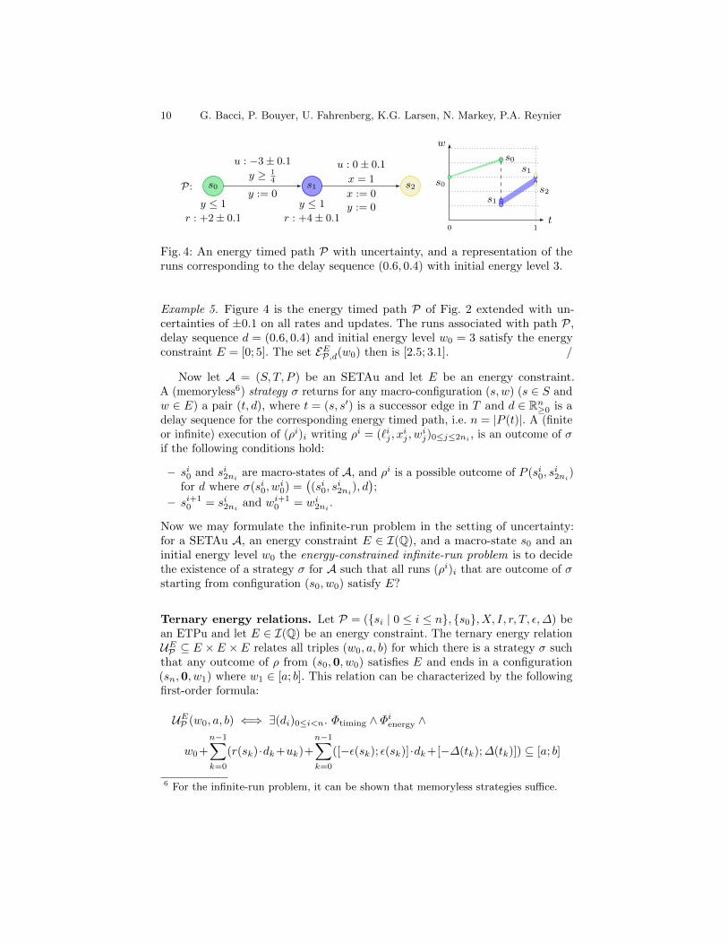
Fig. 4: An energy timed path P with uncertainty, and a representation of theruns corresponding to the delay sequence (0.6, 0.4) with initial energy level 3.

Example 5. Figure 4 is the energy timed path P of Fig. 2 extended with un-certainties of ±0.1 on all rates and updates. The runs associated with path P,delay sequence d = (0.6, 0.4) and initial energy level w0 = 3 satisfy the energyconstraint E = [0; 5]. The set EEP,d(w0) then is [2.5; 3.1]. /

Now let A = (S, T, P ) be an SETAu and let E be an energy constraint.A (memoryless6) strategy σ returns for any macro-configuration (s, w) (s ∈ S andw ∈ E) a pair (t, d), where t = (s, s′) is a successor edge in T and d ∈ Rn≥0 is adelay sequence for the corresponding energy timed path, i.e. n = |P (t)|. A (finiteor infinite) execution of (ρi)i writing ρi = (ìj , x

ij , w

ij)0≤j≤2ni

, is an outcome of σif the following conditions hold:

– si0 and si2niare macro-states of A, and ρi is a possible outcome of P (si0, s

i2ni

)for d where σ(si0, w

i0) =

((si0, s

i2ni

), d);

– si+10 = si2ni

and wi+10 = wi2ni

.

Now we may formulate the infinite-run problem in the setting of uncertainty:for a SETAu A, an energy constraint E ∈ I(Q), and a macro-state s0 and aninitial energy level w0 the energy-constrained infinite-run problem is to decidethe existence of a strategy σ for A such that all runs (ρi)i that are outcome of σstarting from configuration (s0, w0) satisfy E?

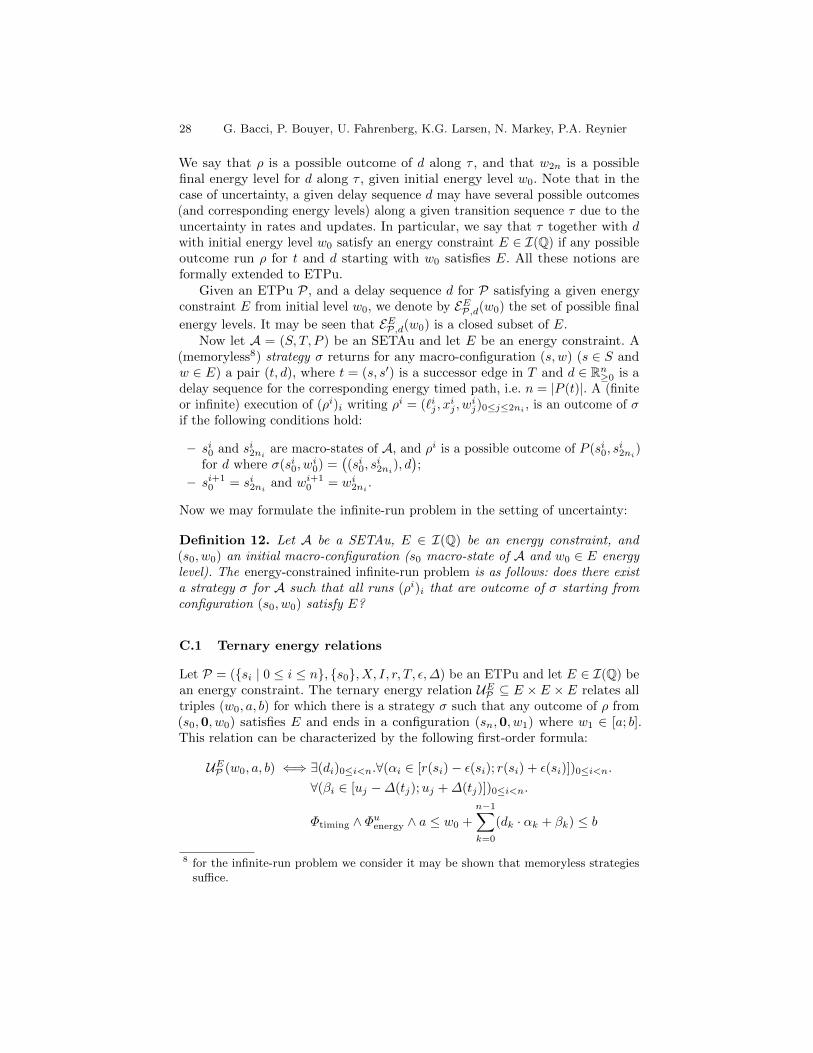
Ternary energy relations. Let P = ({si | 0 ≤ i ≤ n}, {s0}, X, I, r, T, ε,∆) bean ETPu and let E ∈ I(Q) be an energy constraint. The ternary energy relationUEP ⊆ E ×E ×E relates all triples (w0, a, b) for which there is a strategy σ suchthat any outcome of ρ from (s0,0, w0) satisfies E and ends in a configuration(sn,0, w1) where w1 ∈ [a; b]. This relation can be characterized by the followingfirst-order formula:

UEP (w0, a, b) ⇐⇒ ∃(di)0≤i<n. Φtiming ∧ Φienergy ∧

w0 +

n−1∑

k=0

(r(sk)·dk+uk)+

n−1∑

k=0

([−ε(sk); ε(sk)]·dk+[−∆(tk);∆(tk)]) ⊆ [a; b]

6 For the infinite-run problem, it can be shown that memoryless strategies suffice.


where Φienergy encodes the energy constraints as the inclusion of the interval ofreachable energy levels in the energy constraint (in the same way as we do on thesecond line of the formula). Interval inclusion can then be expressed as constraintson the bounds of the intervals. It is clear that UEP is a closed, convex subset ofE ×E ×E and can be described as a finite conjunction of linear constraints overw0, a and b using quantifier elimination.

Example 6. We illustrate the above translation on the ETPu of Fig. 4. For energyconstraint [0; 5], the energy relation can be written as:

UEP (w0, a, b) ⇐⇒ ∃d0, d1. d0 ∈ [0.25; 1] ∧ d1 ∈ [0; 1] ∧ d0 + d1 = 1 ∧ w0 ∈ [0; 5] ∧w0 + [1.9; 2.1] · d0 ⊆ [0; 5] ∧w0 + [1.9; 2.1] · d0 + [−3.1;−2.9] ⊆ [0; 5] ∧w0 + [1.9; 2.1] · d0 + [−3.1;−2.9] + [3.9; 4.1] · d1 ⊆ [0; 5] ∧w0 + [1.9; 2.1] · d0 + [−3.1;−2.9] + [3.9; 4.1] · d1 + [−0.1; 0.1] ⊆ [a; b] ⊆ [0; 5]]

Applying quantifier elimination, we end up with:

UEP (w0, a, b) ⇐⇒ 0 ≤ a ≤ b ≤ 5 ∧ b ≥ a+ 0.6 ∧ a− 0.2 ≤ w0 ≤ b+ 0.7 ∧(4.87 + 1.9 · a)/3.9 ≤ w0 ≤ (7.27 + 2.1 · b)/4.1

We can use this relation in order to compute the set of initial energy levels fromwhich there is a strategy to end up in [2.5; 3.1] (which was the set of possiblefinal energy levels in the example of Fig. 4). We get w0 ∈ [37/15; 689/205], whichis (under-)approximately w0 ∈ [2.467; 3.360]. /

Algorithm for SETAu. Let A = (S, T, P ) be a SETAu and let E ∈ I(Q)be an energy constraint. Let W ⊆ S × E be the maximal set of configurationssatisfying the following:

(s, w) ∈ W ⇒∃t = (s, s′) ∈ T.∃a, b ∈ E.UEP (t)(w, a, b) ∧ ∀w′ ∈ [a; b].(s′, w′) ∈ W (2)

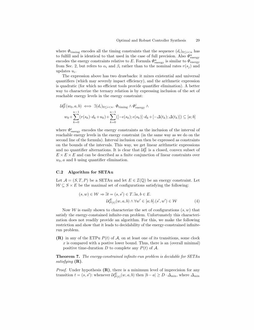
NowW is easily shown to characterize the set of configurations (s, w) that satisfythe energy-constrained infinite-run problem. Unfortunately this characterizationdoes not readily provide an algorithm. We thus make the following restriction andshow that it leads to decidability of the energy-constrained infinite-run problem:

(R) in any of the ETPu P (t) of A, on at least one of its transitions, some clock xis compared with a positive lower bound. Thus, there is an (overall minimal)positive time-duration D to complete any P (t) of A.

Theorem 7. The energy-constrained infinite-run problem is decidable for SETAusatisfying (R).


It is worth noticing that we do not assume flatness of the model for provingthe above theorem. Instead, the minimal-delay assumption (R) has to be made:it entails that any stable set is made of intervals whose size is bounded below,which provides an upper bound on the number of such intervals. We can thenrewrite the right-hand-size expression of (2) as:

∧

s∈S

∧

1≤j≤N[as,j ; bs,j ] ⊆ E ∧ w0 ∈

∨

1≤j≤N[as0,j ; bs0,j ] ∧ ∀w ∈ [as,j ; bs,j ].

∨

(s,s′)∈T

[∃a, b ∈ E. UEP (s,s′)(w, a, b) ∧

∨

1≤k≤N([a; b] ⊆ [as′,k; bs′,k])

](3)

Example 7. We pursue on Example 6. If ETPu P is iterated (as on the loopon state s2 of Fig. 3, but now with uncertainty), the set W (there is a singlemacro-state) can be captured with a single interval [a, b]. We characterize theset of energy levels from which the path P can be iterated infinitely often whilesatisfying the energy constraint E = [0; 5] using equation (3), as follows:

0 ≤ a ≤ b ≤ 5 ∧ ∀w0 ∈ [a; b]. UEP (w0, a, b).

We end up with 2.435 ≤ a ∧ b ≤ 3.635 ∧ b ≥ a+ 0.6, so that the largest intervalis [2.435; 3.635] (which can be compared to the maximal fixpoint [2; 4] that weobtained in Example 4 for the same cycle without uncertainty). /

As in the setting without uncertainties, we can also synthesize an (optimal)upper-bound for the energy constraint:

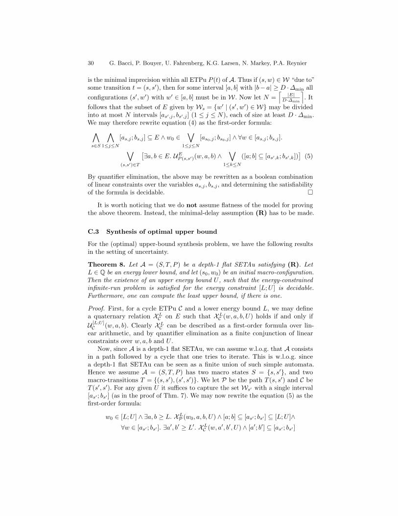
Theorem 8. Let A = (S, T, P ) be a depth-1 flat SETAu satisfying (R). LetL ∈ Q be an energy lower bound, and let (s0, w0) be an initial macro-configuration.Then the existence of an upper energy bound U , such that the energy-constrainedinfinite-run problem is satisfied for the energy constraint [L;U ] is decidable.Furthermore, one can compute the least upper bound, if there is one.

4 Case Study

Modelling the Oil Pump System. In this section we describe the character-istics of each component of the HYDAC case, which we then model as a SETA.

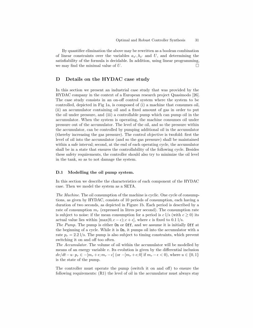
The Machine. The oil consumption of the machine is cyclic. One cycle of consump-tions, as given by HYDAC, consists of 10 periods of consumption, each having aduration of two seconds, as depicted in Figure 1b. Each period is described by arate of consumption mr (expressed in litres per second). The consumption rateis subject to noise: if the mean consumption for a period is c l/s (with c ≥ 0) itsactual value lies within [max(0, c− ε); c+ ε], where ε is fixed to 0.1 l/s.The Pump. The pump is either On or Off, and we assume it is initially Off atthe beginning of a cycle. While it is On, it pumps oil into the accumulator with arate pr = 2.2 l/s. The pump is also subject to timing constraints, which preventswitching it on and off too often.


The Accumulator. The volume of oil within the accumulator will be modelled bymeans of an energy variable v. Its evolution is given by the differential inclusiondv/dt−u ·pr ∈ −[mr + ε;mr− ε] (or −[mr + ε; 0] if mr− ε < 0), where u ∈ {0, 1}is the state of the pump.

The controller must operate the pump (switch it on and off) to ensure thefollowing requirements: (R1) the level of oil in the accumulator must always staywithin the safety bounds E = [Vmin;Vmax] = [4.9; 25.1] l (R2) the average level ofoil in the accumulator is kept as low as possible.

By modelling the oil pump system as a SETA H, the above control problemcan be reduced to finding a deterministic schedule that results in a safe infiniterun in H. Furthermore, we are also interested in determining the minimal safetyinterval E, i.e., finding interval bounds that minimize Vmax−Vmin, while ensuringthe existence of a valid controller for H.

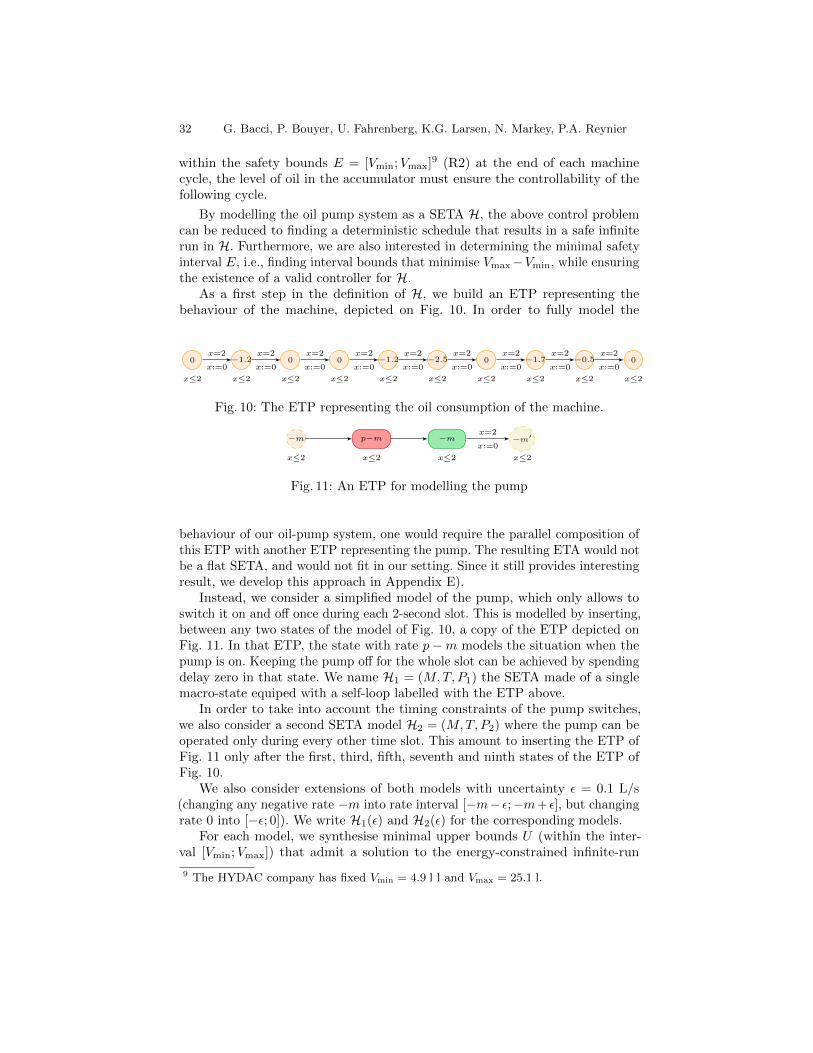
As a first step in the definition of H, we build an ETP representing thebehaviour of the machine, depicted on Fig. 5. In order to fully model the behaviour

0

x≤2

−1.2

x≤2

0

x≤2

0

x≤2

−1.2

x≤2

−2.5

x≤2

0

x≤2

−1.7

x≤2

−0.5

x≤2

0

x≤2

x=2

x:=0

x=2

x:=0

x=2

x:=0

x=2

x:=0

x=2

x:=0

x=2

x:=0

x=2

x:=0

x=2

x:=0

x=2

x:=0

Fig. 5: The ETP representing the oil consumption of the machine.

−m

x≤2

p−m

x≤2

−m

x≤2

−m′

x≤2

x=2

x:=0

Fig. 6: An ETP for modelling the pump

of our oil-pump system, one would require the parallel composition of this ETPwith another ETP representing the pump. The resulting ETA would not be aflat SETA, and is too large to be handled by our algorithm with uncertainty.Since it still provides interesting results, we develop this (incomplete) approachin Appendix E.

Instead, we consider an alternative model of the pump, which only allows toswitch it on and off once during each 2-second slot. This is modelled by inserting,between any two states of the model of Fig. 5, a copy of the ETP depicted onFig. 6. In that ETP, the state with rate p −m models the situation when thepump is on. Keeping the pump off for the whole slot can be achieved by spendingdelay zero in that state. We name H1 = (M,T, P1) the SETA made of a singlemacro-state equipped with a self-loop labelled with the ETP above.

In order to represent the timing constraints of the pump switches, we alsoconsider a second SETA model H2 = (M,T, P2) where the pump can be operatedonly during every other time slot. This amounts to inserting the ETP of Fig. 6only after the first, third, fifth, seventh and ninth states of the ETP of Fig. 5.

We also consider extensions of both models with uncertainty ε = 0.1 l/s(changing any negative rate −m into rate interval [−m− ε;−m+ ε], but changingrate 0 into [−ε; 0]). We write H1(ε) and H2(ε) for the corresponding models.


0 3 6 9 12 15 18

49

52

55

58

61

64

67

70

time (seconds)

initialvolume(decilitre)

0 3 6 9 12 15 18

49

53

57

61

65

69

73

77

81

85

89

time (seconds)


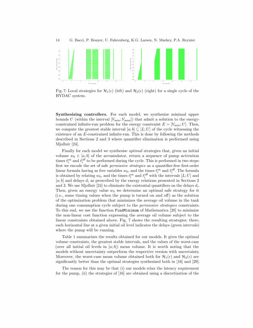
Fig. 7: Local strategies for H1(ε) (left) and H2(ε) (right) for a single cycle of theHYDAC system.

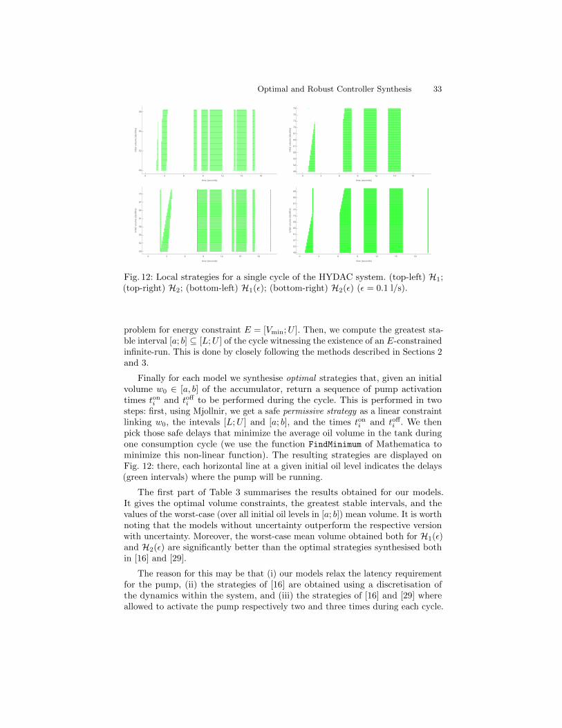
Synthesizing controllers. For each model, we synthesize minimal upperbounds U (within the interval [Vmin;Vmax]) that admit a solution to the energy-constrained infinite-run problem for the energy constraint E = [Vmin;U ]. Then,we compute the greatest stable interval [a; b] ⊆ [L;U ] of the cycle witnessing theexistence of an E-constrained infinite-run. This is done by following the methodsdescribed in Sections 2 and 3 where quantifier elimination is performed usingMjollnir [24].

Finally for each model we synthesise optimal strategies that, given an initialvolume w0 ∈ [a, b] of the accumulator, return a sequence of pump activationtimes ton

i and toffi to be performed during the cycle. This is performed in two steps:

first we encode the set of safe permissive strategies as a quantifier-free first-orderlinear formula having as free variables w0, and the times ton

i and toffi . The formula

is obtained by relating w0, and the times toni and toff

i with the intervals [L;U ] and[a; b] and delays di as prescribed by the energy relations presented in Sections 2and 3. We use Mjollnir [24] to eliminate the existential quantifiers on the delays di.Then, given an energy value w0 we determine an optimal safe strategy for it(i.e., some timing values when the pump is turned on and off) as the solutionof the optimization problem that minimizes the average oil volume in the tankduring one consumption cycle subject to the permissive strategies constraints.To this end, we use the function FindMinimum of Mathematica [28] to minimizethe non-linear cost function expressing the average oil volume subject to thelinear constraints obtained above. Fig. 7 shows the resulting strategies: there,each horizontal line at a given initial oil level indicates the delays (green intervals)where the pump will be running.

Table 1 summarizes the results obtained for our models. It gives the optimalvolume constraints, the greatest stable intervals, and the values of the worst-case(over all initial oil levels in [a; b]) mean volume. It is worth noting that themodels without uncertainty outperform the respective version with uncertainty.Moreover, the worst-case mean volume obtained both for H1(ε) and H2(ε) aresignificantly better than the optimal strategies synthesized both in [16] and [29].

The reason for this may be that (i) our models relax the latency requirementfor the pump, (ii) the strategies of [16] are obtained using a discretization of the


Controller [L;U ] [a; b] Mean vol. (l)

H1 [4.9; 5.84] [4.9; 5.84] 5.43

H1(ε) [4.9; 7.16] [5.1; 7.16] 6.15

H2 [4.9; 7.9] [4.9; 7.9] 6.12

H2(ε) [4.9; 9.1] [5.1; 9.1] 7.24

G1M1 [16] [4.9; 25.1](∗) [5.1; 9.4] 8.2

G2M1 [16] [4.9; 25.1](∗) [5.1; 8.3] 7.95

[29] [4.9; 25.1](∗) [5.2; 8.1] 7.35(∗) Safety interval given by the HYDAC company.

Table 1: Characteristics of the synthesized strategies, compared with the strategiesproposed in [16,29].

0 10 20 30 40 50 60 70 80 90 100

495255586164677073767982858891

time (seconds)

pump[off/on

];volume(decilitre)

0 10 20 30 40 50 60 70 80 90 100

495255586164677073767982858891

time (seconds)

pump[off/on

];volume(decilitre)

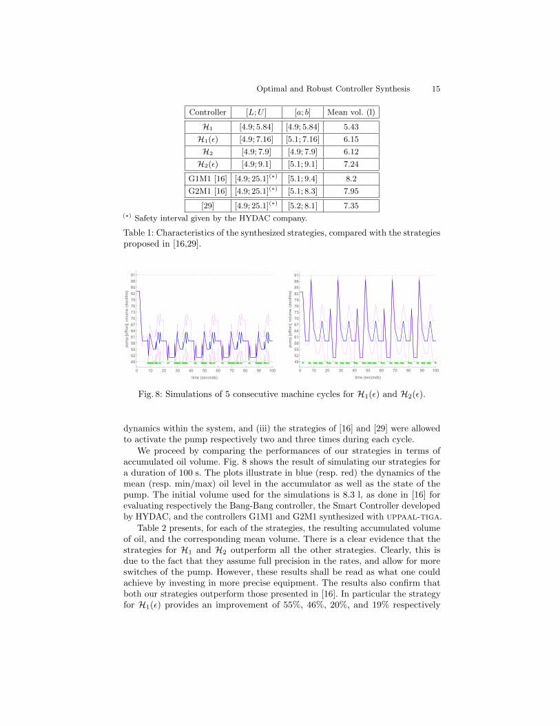
Fig. 8: Simulations of 5 consecutive machine cycles for H1(ε) and H2(ε).

dynamics within the system, and (iii) the strategies of [16] and [29] were allowedto activate the pump respectively two and three times during each cycle.

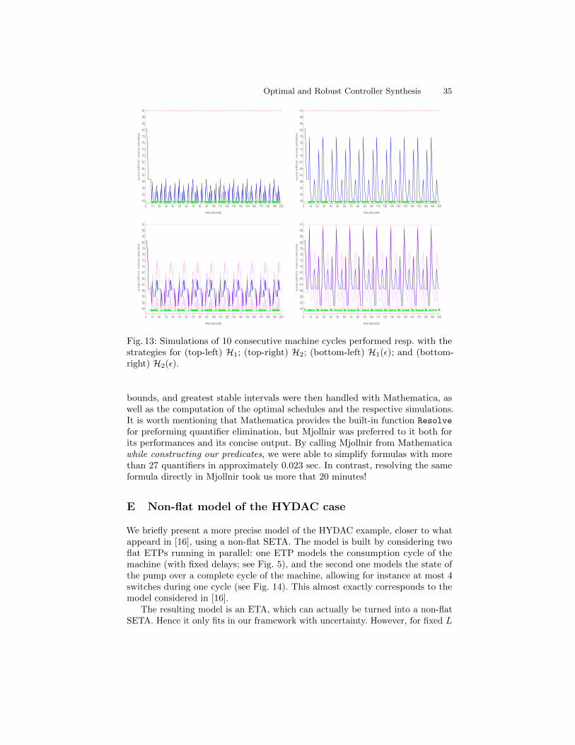
We proceed by comparing the performances of our strategies in terms ofaccumulated oil volume. Fig. 8 shows the result of simulating our strategies fora duration of 100 s. The plots illustrate in blue (resp. red) the dynamics of themean (resp. min/max) oil level in the accumulator as well as the state of thepump. The initial volume used for the simulations is 8.3 l, as done in [16] forevaluating respectively the Bang-Bang controller, the Smart Controller developedby HYDAC, and the controllers G1M1 and G2M1 synthesized with uppaal-tiga.

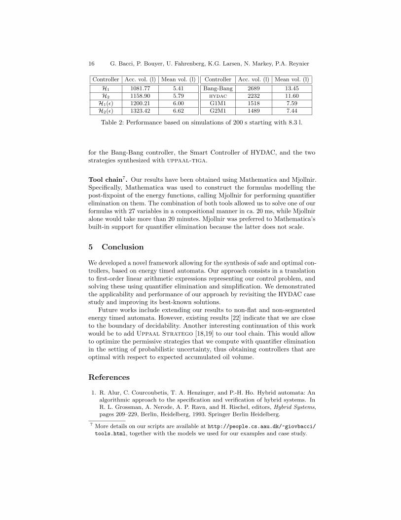
Table 2 presents, for each of the strategies, the resulting accumulated volumeof oil, and the corresponding mean volume. There is a clear evidence that thestrategies for H1 and H2 outperform all the other strategies. Clearly, this isdue to the fact that they assume full precision in the rates, and allow for moreswitches of the pump. However, these results shall be read as what one couldachieve by investing in more precise equipment. The results also confirm thatboth our strategies outperform those presented in [16]. In particular the strategyfor H1(ε) provides an improvement of 55%, 46%, 20%, and 19% respectively


Controller Acc. vol. (l) Mean vol. (l)

H1 1081.77 5.41

H2 1158.90 5.79

H1(ε) 1200.21 6.00

H2(ε) 1323.42 6.62


Bang-Bang 2689 13.45

hydac 2232 11.60

G1M1 1518 7.59

G2M1 1489 7.44

Table 2: Performance based on simulations of 200 s starting with 8.3 l.

for the Bang-Bang controller, the Smart Controller of HYDAC, and the twostrategies synthesized with uppaal-tiga.

Tool chain7. Our results have been obtained using Mathematica and Mjollnir.Specifically, Mathematica was used to construct the formulas modelling thepost-fixpoint of the energy functions, calling Mjollnir for performing quantifierelimination on them. The combination of both tools allowed us to solve one of ourformulas with 27 variables in a compositional manner in ca. 20 ms, while Mjollniralone would take more than 20 minutes. Mjollnir was preferred to Mathematica’sbuilt-in support for quantifier elimination because the latter does not scale.

5 Conclusion

We developed a novel framework allowing for the synthesis of safe and optimal con-trollers, based on energy timed automata. Our approach consists in a translationto first-order linear arithmetic expressions representing our control problem, andsolving these using quantifier elimination and simplification. We demonstratedthe applicability and performance of our approach by revisiting the HYDAC casestudy and improving its best-known solutions.

Future works include extending our results to non-flat and non-segmentedenergy timed automata. However, existing results [22] indicate that we are closeto the boundary of decidability. Another interesting continuation of this workwould be to add Uppaal Stratego [18,19] to our tool chain. This would allowto optimize the permissive strategies that we compute with quantifier eliminationin the setting of probabilistic uncertainty, thus obtaining controllers that areoptimal with respect to expected accumulated oil volume.

References

1. R. Alur, C. Courcoubetis, T. A. Henzinger, and P.-H. Ho. Hybrid automata: Analgorithmic approach to the specification and verification of hybrid systems. InR. L. Grossman, A. Nerode, A. P. Ravn, and H. Rischel, editors, Hybrid Systems,pages 209–229, Berlin, Heidelberg, 1993. Springer Berlin Heidelberg.

7 More details on our scripts are available at http://people.cs.aau.dk/~giovbacci/tools.html, together with the models we used for our examples and case study.

http://people.cs.aau.dk/~giovbacci/tools.html

http://people.cs.aau.dk/~giovbacci/tools.html


2. R. Alur and D. L. Dill. A theory of timed automata. Theoretical Computer Science,126(2):183–235, Apr. 1994.

3. R. Alur, S. La Torre, and G. J. Pappas. Optimal paths in weighted timed automata.In M. D. Di Benedetto and A. L. Sangiovani-Vincentelli, editors, Proceedings ofthe 4th International Workshop on Hybrid Systems: Computation and Control(HSCC’01), volume 2034 of Lecture Notes in Computer Science, pages 49–62.Springer-Verlag, Mar. 2001.

4. G. Bacci, P. Bouyer, U. Fahrenberg, K. G. Larsen, N. Markey, and P.-A. Reynier.Optimal and Robust Controller Synthesis: Using Energy Timed Automata withUncertainty, 2018. arXiv:1805.00847 [cs.FL].

5. G. Behrmann, A. Cougnard, A. David, E. Fleury, K. G. Larsen, and D. Lime.UPPAAL-Tiga: Time for playing games! In W. Damm and H. Hermanns, editors,Computer Aided Verification, 19th International Conference, CAV 2007, Berlin,Germany, July 3-7, 2007, Proceedings, volume 4590 of Lecture Notes in ComputerScience, pages 121–125. Springer, 2007.

6. G. Behrmann, A. Fehnker, T. Hune, K. G. Larsen, P. Pettersson, J. Romijn, andF. Vaandrager. Minimum-cost reachability for priced timed automata. In M. D.Di Benedetto and A. L. Sangiovani-Vincentelli, editors, Proceedings of the 4thInternational Workshop on Hybrid Systems: Computation and Control (HSCC’01),volume 2034 of Lecture Notes in Computer Science, pages 147–161. Springer-Verlag,Mar. 2001.

7. A. Bemporad, G. Ferrari-Trecate, and M. Morari. Observability and controllabilityof piecewise affine and hybrid systems. IEEE Transactions on Automatic Control,45(10):1864–1876, 2000.

8. M. Bisgaard, D. Gerhardt, H. Hermanns, J. Krcal, G. Nies, and M. Stenger. Battery-aware scheduling in low orbit: The GomX-3 case. In J. S. Fitzgerald, C. L. Heitmeyer,S. Gnesi, and A. Philippou, editors, FM 2016: Formal Methods - 21st InternationalSymposium, Limassol, Cyprus, November 9-11, 2016, Proceedings, volume 9995 ofLecture Notes in Computer Science, pages 559–576, 2016.

9. V. D. Blondel, O. Bournez, P. Koiran, and J. N. Tsitsiklis. The stability of saturatedlinear dynamical systems is undecidable. Journal of Computer and System Sciences,62(3):442–462, 2001.

10. V. D. Blondel and J. N. Tsitsiklis. Complexity of stability and controllability ofelementary hybrid systems. Automatica, 35(3):479–489, 1999.

11. P. Bouyer, U. Fahrenberg, K. G. Larsen, and N. Markey. Timed automata withobservers under energy constraints. In K. H. Johansson and W. Yi, editors,Proceedings of the 13th International Workshop on Hybrid Systems: Computationand Control (HSCC’10), pages 61–70. ACM Press, Apr. 2010.

12. P. Bouyer, U. Fahrenberg, K. G. Larsen, N. Markey, and J. Srba. Infinite runs inweighted timed automata with energy constraints. In F. Cassez and C. Jard, editors,Proceedings of the 6th International Conferences on Formal Modelling and Analysisof Timed Systems (FORMATS’08), volume 5215 of Lecture Notes in ComputerScience, pages 33–47. Springer-Verlag, Sept. 2008.

13. P. Bouyer, K. G. Larsen, and N. Markey. Lower-bound constrained runs in weightedtimed automata. Performance Evaluation, 73:91–109, Mar. 2014.

14. M. Bozga, R. Iosif, and Y. Lakhnech. Flat parametric counter automata. InM. Bugliesi, B. Preneel, V. Sassone, and I. Wegener, editors, Proceedings of the 33rdInternational Colloquium on Automata, Languages and Programming (ICALP’06)) –Part II, volume 4052 of Lecture Notes in Computer Science, pages 577–588. Springer-Verlag, July 2006.


15. F. Cassez, A. David, E. Fleury, K. G. Larsen, and D. Lime. Efficient on-the-flyalgorithms for the analysis of timed games. In M. Abadi and L. de Alfaro, editors,CONCUR 2005 - Concurrency Theory, 16th International Conference, CONCUR2005, San Francisco, CA, USA, August 23-26, 2005, Proceedings, volume 3653 ofLecture Notes in Computer Science, pages 66–80. Springer, 2005.

16. F. Cassez, J. J. Jensen, K. G. Larsen, J.-F. Raskin, and P.-A. Reynier. Automaticsynthesis of robust and optimal controllers – an industrial case study. In R. Ma-jumdar and P. Tabuada, editors, Proceedings of the 12th International Workshopon Hybrid Systems: Computation and Control (HSCC’09), volume 5469 of LectureNotes in Computer Science, pages 90–104. Springer-Verlag, Apr. 2009.

17. H. Comon and Y. Jurski. Multiple counters automata, safety analysis, and Pres-burger arithmetic. In A. J. Hu and M. Y. Vardi, editors, Proceedings of the 10thInternational Conference on Computer Aided Verification (CAV’98), volume 1427of Lecture Notes in Computer Science, pages 268–279. Springer-Verlag, June-July1998.

18. A. David, P. G. Jensen, K. G. Larsen, A. Legay, D. Lime, M. G. Sørensen, and J. H.Taankvist. On time with minimal expected cost! In F. Cassez and J. Raskin, editors,Automated Technology for Verification and Analysis - 12th International Symposium,ATVA 2014, Sydney, NSW, Australia, November 3-7, 2014, Proceedings, volume8837 of Lecture Notes in Computer Science, pages 129–145. Springer, 2014.

19. A. David, P. G. Jensen, K. G. Larsen, M. Mikucionis, and J. H. Taankvist. Up-paal Stratego. In C. Baier and C. Tinelli, editors, Tools and Algorithms for theConstruction and Analysis of Systems - 21st International Conference, TACAS2015, Held as Part of the European Joint Conferences on Theory and Practice ofSoftware, ETAPS 2015, London, UK, April 11-18, 2015. Proceedings, volume 9035of Lecture Notes in Computer Science, pages 206–211. Springer, 2015.

20. G. Frehse. Phaver: algorithmic verification of hybrid systems past hytech. STTT,10(3):263–279, 2008.

21. S. Jha, S. A. Seshia, and A. Tiwari. Synthesis of optimal switching logic for hybridsystems. In S. Chakraborty, A. Jerraya, S. K. Baruah, and S. Fischmeister, editors,Proceedings of the 11th International Conference on Embedded Software, EMSOFT2011, part of the Seventh Embedded Systems Week, ESWeek 2011, Taipei, Taiwan,October 9-14, 2011, pages 107–116. ACM, 2011.

22. N. Markey. Verification of Embedded Systems – Algorithms and Complexity. Memoired’habilitation, Ecole Normale Superieure de Cachan, France, Apr. 2011.

23. S. Miremadi, Z. Fei, K. Akesson, and B. Lennartson. Symbolic supervisory controlof timed discrete event systems. IEEE Trans. Contr. Sys. Techn., 23(2):584–597,2015.

24. D. Monniaux. Quantifier elimination by lazy model enumeration. In T. Touili,B. Cook, and P. B. Jackson, editors, Computer Aided Verification, 22nd Inter-national Conference, CAV 2010, Edinburgh, UK, July 15-19, 2010. Proceedings,volume 6174 of Lecture Notes in Computer Science, pages 585–599. Springer, 2010.

25. A. Phan, M. R. Hansen, and J. Madsen. EHRA: Specification and analysis ofenergy-harvesting wireless sensor networks. In S. Iida, J. Meseguer, and K. Ogata,editors, Specification, Algebra, and Software - Essays Dedicated to Kokichi Futatsugi,volume 8373 of Lecture Notes in Computer Science, pages 520–540. Springer, 2014.

26. Quasimodo. Quantitative system properties in model-driven design of embeddedsystems. http://www.quasimodo.aau.dk/.

27. G. von Bochmann, M. Hilscher, S. Linker, and E. Olderog. Synthesizing and verifyingcontrollers for multi-lane traffic maneuvers. Formal Asp. Comput., 29(4):583–600,2017.

http://www.quasimodo.aau.dk/


28. Wolfram Research, Inc. Mathematica, Version 11.2. Champaign, IL, 2017.29. H. Zhao, N. Zhan, D. Kapur, and K. G. Larsen. A “hybrid” approach for synthesizing

optimal controllers of hybrid systems: A case study of the oil pump industrialexample. In D. Giannakopoulou and D. Mery, editors, FM 2012: Formal Methods- 18th International Symposium, Paris, France, August 27-31, 2012. Proceedings,volume 7436 of Lecture Notes in Computer Science, pages 471–485. Springer, 2012.


A Proof of Theorem 3

Binary energy relations. Let P = ({si | 0 ≤ i ≤ n}, {s0}, X, I, r, T ) be anETP from s0 to sn. Let E ⊆ I(Q) be an energy constraint. The binary energyrelation REP ⊆ E ×E for P under energy constraint E relates all pairs (w0, w1)for which there is a finite run of P from (s0,0, w0) to (sn,0, w1) satisfying energyconstraint E. This relation is characterized by the following first-order formula:

REP(w0, w1) ⇐⇒ ∃(di)0≤i<n. Φtiming ∧ Φenergy ∧ w1 = w0 +

n−1∑

k=0

(dk · r(sk) + uk)

where Φtiming encodes all the timing constraints that the sequence (di)0≤i<n hasto fulfill, while Φenergy encodes the energy constraints. More precisely:

– timing constraints are obtained by computing the clock valuations in eachstate of the execution, and expressing that those values must satisfy thecorresponding invariants and guards. The value of a clock in a state is thesum of the delays dj since the last reset of that clock along the ETP.

– energy constraints are obtained by expressing the value of the energy level ineach state as the sum of the initial energy level, the energy r(si) ·di gained orconsumed in each intermediary state, and the updates ui of the transitionsthat have been traversed. All those values are constrained to lie in E.

It is easily shown that REP is a closed, convex subset of E×E (remember thatwe consider closed clock constraints); thus it can be described as a conjunctionof a finite set of linear constraints over w0 and w1 (with non-strict inequalities),using quantifier elimination of variables (di)0≤i<n.

Energy functions. We now focus on properties of energy relations. First noticethat for any interval E ∈ I(Q), the partially-ordered set (I(E),⊇) is ω-complete,meaning that for any chain (Ij)j∈N, with Ij ⊇ Ij+1 for all j, the limit

⋂j∈N Ij

also belongs to I(E). By Cantor’s Intersection Theorem, if additionally eachinterval Ij is non-empty, then so is the limit

⋂j∈N Ij .

With an energy relation REP , we associate an energy function (also denotedwith REP , or simply R, as long as no ambiguity may arise), defined for any closedsubinterval I ∈ I(E) as

R(I) = {w1 ∈ E | ∃w0 ∈ I. R(w0, w1)}.

Symmetrically, we let

R−1(I) = {w0 ∈ E | ∃w1 ∈ I. R(w0, w1)}.

Observe that R(I) and R−1(I) also belong to I(E) (because relation R is closedand convex). Moreover, R and R−1 are monotonic: for any two intervals I and Jin I(E) such that I ⊆ J , it holds R(I) ⊆ R(J) and R−1(I) ⊆ R−1(J).

Energy functions R and R−1 also satisfy the following continuity properties:


Lemma 5. Let (Ij)j∈N be a chain of intervals of I(E), such that Ij ⊇ Ij+1 forall j ∈ N. Then R−1(

⋂j∈N Ij) =

⋂j∈NR−1(Ij).

Proof. For any i ∈ N, we have Ii ⊇⋂j∈N Ij . By monotonicity of R−1, we get

R−1(Ii) ⊇ R−1(⋂j∈N Ij). It follows

⋂i∈NR−1(Ii) ⊇ R−1(

⋂j∈N Ij).

Now, let w0 ∈⋂j∈NR−1(Ij). Then for all i ∈ N, there exists wi1 such that

R(w0, wi1). It follows that for any i ∈ N, R({w0}) ∩ Ii is a non-empty interval

of I(E). Applying Cantor’s Intersection Theorem, we get that⋂i∈NR({w0})∩ Ii

is a non-empty interval of I(E). This intersection can be rewritten as R({w0})∩⋂i∈N Ii; hence there exists w1 ∈

⋂i∈N Ii such that R(w0, w1), which proves that

w0 ∈ R−1(⋂i∈N Ii). �

Composition and fixpoints of energy functions. Consider a finite sequenceof paths (Pi)1≤i≤k. Clearly, the energy relation for this sequence can be obtainedas the composition of the individual energy relations REPk

◦· · ·◦REP1; the resulting

energy relation still is a closed convex subset of E ×E that can be described asthe conjunction of finitely many linear constraints over w0 and w1. As a specialcase, we write (REP)k for the composition of k copies of the same relations REP .

Now, using Lemma 5, we easily prove that the greatest fixpoint νR−1 of R−1

in the complete lattice (I(E),⊇) exists and equals:

νR−1 =⋂

i∈N(R−1)i(E).

Moreover νR−1 is a closed (possibly empty) interval. Note that νR−1 is themaximum subset SR of E such that, starting with any w0 ∈ SR, it is possible toiterate R infinitely many times (that is, for any w0 ∈ SR, there exists w1 ∈ SRsuch that R(w0, w1)—any such set S is a post-fixpoint of R−1 in the sense thatS ⊆ R−1(S)).

In the end, if R is the energy relation of a cycle C in the SETA, then νR−1

precisely describes the set of initial energy levels allowing infinite runs through Csatisfying the energy constraint E.

Now if R is the energy relation for a cycle C, described as the conjunction φCof a finite set of linear constraints, we can characterize those intervals [a, b] ⊆ Ethat constitute a post-fixpoint for R−1 by the following first-order formula:

a ≤ b ∧ a ∈ E ∧ b ∈ E ∧ ∀w0 ∈ [a; b]. ∃w1 ∈ [a; b]. φC(w0, w1).

Applying quantifier eliminination (to w0 and w1), the above formula may betransformed into a direct constraint on a and b, characterizing all post-fixpointsof R−1. We get a characterization of νR−1 by computing the values of a and bthat satisfy these constraint and maximize b− a.

Algorithm for flat segmented energy timed automata. Following Exam-ple 4, we now prove that we can solve the energy-constrained infinite-run problemfor any flat SETA. The next theorem is crucial for our algorithm:


Theorem 6. Let R be the energy relation of an ETP P with energy constraint E,and let I ∈ I(E). Then either I ∩ νR−1 6= ∅ or Rn(I) = ∅ for some n.

Proof. Assume that I ∩ νR−1 = ∅. Then:

∅ = I ∩ νR−1

= I ∩⋂n∈N(R−1

)n(E)

= I ∩⋂n∈N(Rn)−1

(E) (by R−1 ◦ R−1 = (R ◦R)−1)

=⋂n∈N

(I ∩

(Rn)−1

(E))

Note that(I∩(Rn)−1(E)

)n∈N is a decreasing sequence because

((R−1)n(E)

)n∈N is.

Therefore, by Cantor’s intersection theorem I ∩(Rn)−1

(E) = ∅ for some n ∈ N.

But only elements w0 ∈(Rn)−1

(E) admit some w1 ∈ E such that Rn(w0, w1).Therefore Rn(I) = ∅. �

We will show that the energy-constrained infinite run problem is decidable forflat SETAs. The decision procedure traverses the underlying graph of A, forwardpropagating an initial energy interval I0 ⊆ E looking for a simple cycle C suchthat νR−1

C ∩ I 6= ∅, where I ⊆ E is the energy interval forward-propagated untilreaching the cycle.

Algorithm 2 gives a detailed description of the decision procedure. The pro-cedure traverses the underlying graph of the flat SETA A, namely G = (S, T ),using a waiting list W to keep track of the macro-states that need to be furtherexplored. The list W contains tasks of the form (m, I,flag) where m ∈ S is thecurrent macro-state, I ∈ I(E) is the current energy interval, and flag ∈ {c, c} is aflag indicating if m shall be explored by following a cycle it belongs to (flag = c),or by skipping that cycle (flag = c). The algorithm first initialises the waitinglist with the initial task (cf. line 1).

The main while loop processes each task in the waiting list, as long asthe list is not empty. It picks a task (m, I,flag) from W (line 3). If flag = c,the exploration will continue from macro-states m′ adjacent to m by forwardpropagating the current energy interval I following the timed path P (m,m′)(cf. lines 6-7). Note that the choice of the arcs (m,m′) ensures that m′ does notbelong to the same cycle as m, thus skipping the cycle with m.

Otherwise, if flag = c, the exploration tries to follow the simple cycle thatcontains m. If m does not belong to any cycle the current task will be simplyput back in the waiting list with the opposite flag (cf. line 23). In case m belongsto the simple cycle C = (m1,m2) · · · (mk,mk+1), the energy relation REC is usedto check if for the current energy interval there exists an infinite run along thecycle C. If such is not the case, the cycle will be iterated only finitely many times(cf. lines 15-21). This is done by adding in W the current task with the flag setto c—corresponding to zero executions of the cycle—then for each execution i of C,the cycle is unfolded up its j-th transition and the task (mj+1,REPj

((REC)i(I)), c)is added to the waiting list—corresponding to i executions of C followed by a tail(m1,m2) · · · (mj ,mj+1). Termination of the while loop in lines 17-21 is ensured


Input: A flat SETA A = (S, T, P ); initial state m0 ∈ S; energy interval I01. W ← {(m0, I0, c)} / initialise the waiting list2. while W 6= ∅ do3. pick (m, I,flag) ∈W / pick an element from the waiting list4. W ←W \ (m, I,flag) / remove the element from the waiting list5. if flag = c then / the node m shall be explored without following a cycle6. for each (m,m′) ∈ T that is not part of a simple cycle of (S, T ) do7. W ←W ∪ {(m′,RE

P (m,m′)(I), c)} / add this new task to the waiting list8. else / the node m shall be explored by following a cycle9. if m belongs to a cycle of (S, T ) then

10. let C = (m1,m2) · · · (mk,mk+1) be the simple cycle s.t. m = m1 = mk+1

11. let RC = RP (mk,mk+1) ◦ · · · ◦ RP (m1,m2) / energy relation of the cycle

12. if I ∩ νR−1C 6= ∅ then / check if there is an infinite run via the cycle C

13. return tt

14. else / the cycle can be executed only finitely many times15. W ←W ∪ {(m, I, c)} / add a new task to the waiting list16. i← 0 / initialise the number of cycle executions17. while Ri

C(I) 6= ∅ do / while i-th energy relation is satified18. for 1 ≤ j < k do19. let RPj = RP (mj ,mj+1) ◦ · · · ◦ RP (m1,m2) / unfold C up to mj+1

20. W ←W ∪ {(mj+1,RPj (RiC(I)), c)} / add a task to the waiting list

21. i← i+ 1 / increment the number of cycle executions22. else / m doesn’t belong to a cycle23. W ←W ∪ {(m, I, c)} / add a new task to the waiting list24. return ff / no infinite run could be found

Algorithm 2: Infinite Run

by Theorem 6, and by the flatness assumption on A, which ensures that eachnode m ∈ S belongs to at most one (simple) cycle, so that once the executionhas left the cycle where m belongs to, the exploration won’t visit m again.

Theorem 3. The energy-constrained infinite-run problem is decidable for flatSETA.

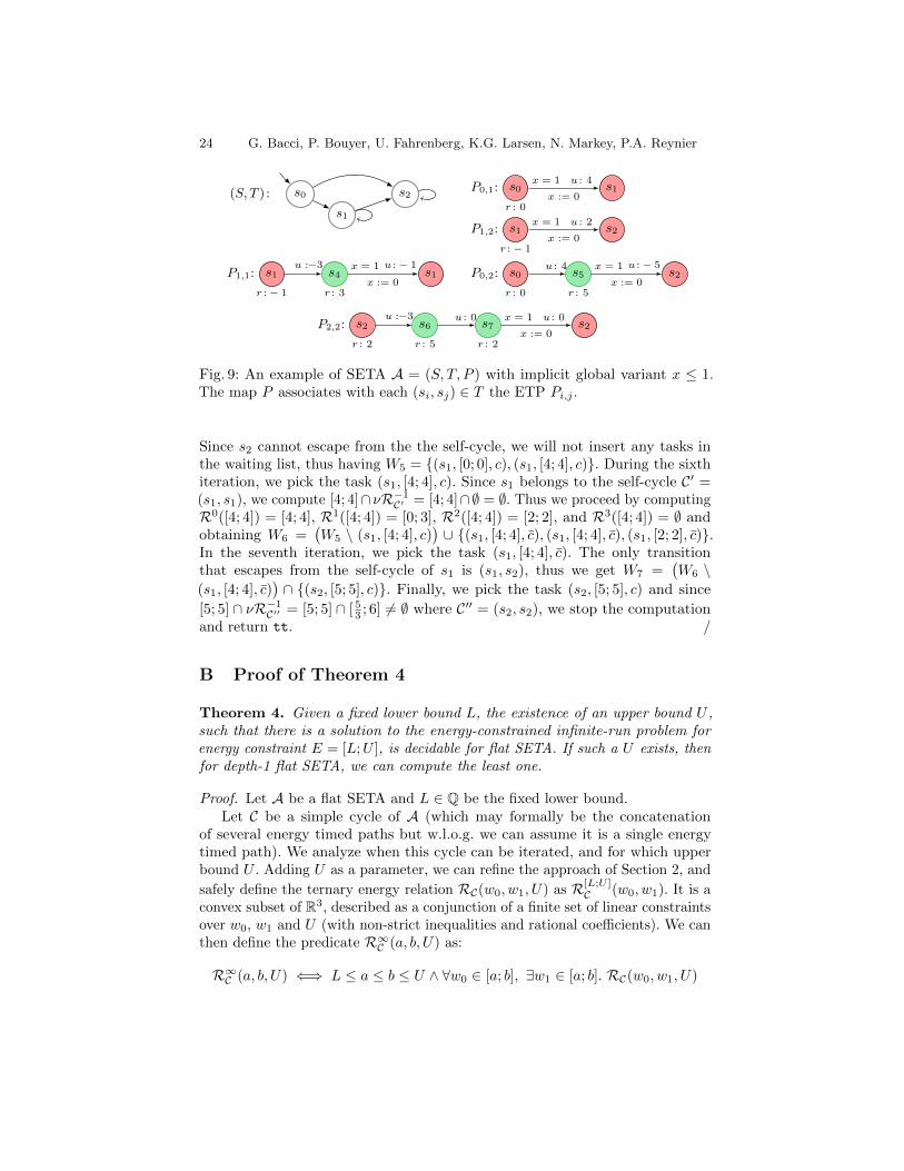
Example 8. Consider the SETA A = (S, T, P ) depicted in Fig. 9 and the energyconstraint E = [0; 6]. We describe a step-by-step execution of Algorithm 2 startingwith s0 ∈ S and initial energy interval I0 = [0; 0].

The waiting list is initialised as W0 = {(s0, I0, c)}. After the first execution ofthe main while loop, W1 = {(s0, I0, c)} because s0 does not belong to any simplecycle of (S, T ). In the second iteration, we pick the task (s0, I0, c) and we updatethe waiting list as W2 = {(s1, [0; 0], c), (s1, [4; 4], c), (s2, [0; 1], c)}. In the thirditeration, we pick the task (s2, [0; 1], c) from W2. Since s2 belongs to the self-cycleC = (s2, s2), we compute [0; 1] ∩ νR−1

C = [0; 1] ∩ [ 53 ; 6] = ∅. Thus, we proceed by

computingR0([0; 1]) = [0; 1],R1([0; 1]) = [0; 0] andR2([0; 1]) = ∅, and update thewaiting list as W3 =

(W2\(s2, [0; 1], c)

)∪{(s2, [0; 1], c), (s2, [0; 0], c)}. In the fourth

and fifth iterations, we pick the tasks (s2, [0; 1], c) and (s2, [0; 0], c), respectively.


s0(S, T ) :

s1

s2

s1

r :− 1

P1,1: s4

r : 3

s1u :−3 u :− 1x = 1

x := 0

s0

r : 0

P0,1: s1u : 4x = 1

x := 0

s1

r :− 1

P1,2: s2u : 2x = 1

x := 0

s0

r : 0

P0,2: s5

r : 5

s2u : 4 u :− 5x = 1

x := 0

s2

r : 2

P2,2: s6

r : 5

s7

r : 2

s2u :−3 u : 0 u : 0x = 1

x := 0

Fig. 9: An example of SETA A = (S, T, P ) with implicit global variant x ≤ 1.The map P associates with each (si, sj) ∈ T the ETP Pi,j .

Since s2 cannot escape from the the self-cycle, we will not insert any tasks inthe waiting list, thus having W5 = {(s1, [0; 0], c), (s1, [4; 4], c)}. During the sixthiteration, we pick the task (s1, [4; 4], c). Since s1 belongs to the self-cycle C′ =(s1, s1), we compute [4; 4]∩ νR−1

C′ = [4; 4]∩∅ = ∅. Thus we proceed by computingR0([4; 4]) = [4; 4], R1([4; 4]) = [0; 3], R2([4; 4]) = [2; 2], and R3([4; 4]) = ∅ andobtaining W6 =

(W5 \ (s1, [4; 4], c)

)∪ {(s1, [4; 4], c), (s1, [4; 4], c), (s1, [2; 2], c)}.

In the seventh iteration, we pick the task (s1, [4; 4], c). The only transitionthat escapes from the self-cycle of s1 is (s1, s2), thus we get W7 =

(W6 \

(s1, [4; 4], c))∩ {(s2, [5; 5], c)}. Finally, we pick the task (s2, [5; 5], c) and since

[5; 5] ∩ νR−1C′′ = [5; 5] ∩ [ 5

3 ; 6] 6= ∅ where C′′ = (s2, s2), we stop the computationand return tt. /

B Proof of Theorem 4

Theorem 4. Given a fixed lower bound L, the existence of an upper bound U ,such that there is a solution to the energy-constrained infinite-run problem forenergy constraint E = [L;U ], is decidable for flat SETA. If such a U exists, thenfor depth-1 flat SETA, we can compute the least one.

Proof. Let A be a flat SETA and L ∈ Q be the fixed lower bound.Let C be a simple cycle of A (which may formally be the concatenation

of several energy timed paths but w.l.o.g. we can assume it is a single energytimed path). We analyze when this cycle can be iterated, and for which upperbound U . Adding U as a parameter, we can refine the approach of Section 2, and

safely define the ternary energy relation RC(w0, w1, U) as R[L;U ]C (w0, w1). It is a

convex subset of R3, described as a conjunction of a finite set of linear constraintsover w0, w1 and U (with non-strict inequalities and rational coefficients). We canthen define the predicate R∞C (a, b, U) as:

R∞C (a, b, U) ⇐⇒ L ≤ a ≤ b ≤ U ∧ ∀w0 ∈ [a; b], ∃w1 ∈ [a; b]. RC(w0, w1, U)


characterizing the intervals [a; b] and upper-bounds U such that C can be iteratedinfinitely many times from any initial value in [a; b] with energy constraint [L;U ].This relation is again a convex subset of R3, described as a conjunction of a finiteset of linear constraints over a, b and U (with non-strict inequalities and rationalcoefficients).

For a fixed U ∈ Q, this predicate coincides with the greatest fixpoint

ν(R[L;U ]C )−1 that was discussed on page 7. Hence R∞C (a, b, U) holds if and only

if for every w0 ∈ [a; b], there is an infinite run starting at (s0,0, w0) (where s0 isthe first state of C) satisfying the energy constraint [L;U ]. Furthermore, sincea ≥ L and L is fixed, and because we only have non-strict constraints, there isa least value aCmin ∈ Q such that the set {(b, U) | R∞C (aCmin, b, U)} is non-empty.In particular:

Lemma 9. – For any energy level w < aCmin, and for any U , there are noinfinite run from (s0,0, w) cycling around C and satisfying energy con-straint [L;U ];

– For every w ≥ aCmin, there exist U and an infinite run from (s0,0, w) cyclingaround C and satisfying energy constraint [L;U ].

Proof. The first part of the lemma is a direct consequence of the analysis of the

fixpoint ν(R[L;U ]C

)−1

made in Sec. 2.

For the second property, we first realize that there is (b, U) ∈ Q2 such thatR∞C (aCmin, b, U), which means in particular that there is an infinite run from(s0,0, a

Cmin) cycling around C and satisfying the energy constraint [L;U ]. Now,

by mimicking the same delays, it is easy to get that for every w ≥ aCmin, there isan infinite run from (s0,0, w) satisfying the energy constraint [L;U +w− aCmin].

�

Coming back to our automaton A: if there is a solution to the energy-constrained infinite-run problem in A for some upper bound U , the witnessinfinite run must end up cycling in one of the cycles of A. Let C be a cycle. Weknow from the lemma above that, to be able to generate a witness infinite runcycling around C, one needs to be able to reach the start of that cycle with atleast energy level aCmin. Note that if we find a finite run reaching the start ofcycle C with energy level w ≥ aCmin and satisfying the energy constraint [L; +∞)(only a lower bound constraint) along the way, then for some U ′ this finite pathsatisfies the energy constaint [L;U ′]; the concatenation of that finite run with awitness infinite run cycling along C while satisfying some [L;U ]-energy constraintgives a witness infinite run for the existence of an upper bound (with upperbound max(U ;U ′)).

We therefore study finite runs leading to the start of cycle C, with only thelower bound L on the energy level. Recall that this problem is in general noteasy to solve [13], and only single-clock automata can be handled in general [11].However in the special setting of flat SETA, we are able to decide the existenceof a well-adapted finite run reaching the start of cycle C. Let P be an energytimed path. Following a similar approach to the approach developed on page 6,


one can easily define a predicate SP(w0, w1) that is true whenever there is arun satisfying the energy constraint [L; +∞), starting with energy level w0 andending with energy level w1. From that predicate, one can derive the predicatesS↑P(w0) (resp. S=

P (w0), S×P (w0)) such that:

– S↑P(w0) ⇐⇒ ∃w1 > w0 s.t. SP(w0, w1);

– S=P (w0) ⇐⇒ SP(w0, w0) and ¬S↑P(w0);

– S×P (w0) ⇐⇒ ∀w1 ≥ w0, ¬SP(w0, w1).

In the two first cases, and only in these cases, the path can be iterated whilesatisfying the energy constraint [L; +∞). In the first case, by iterating the path,one can increase the energy level up to an arbitrarily high value. In the secondcase, only energy level w0 can be reached. These properties are very easy to prove(since there is no upper bound), and are therefore omitted.

Let A be a SETA with initial energy level w0. We perform the following(partial) labelling λ of the graph in a forward manner:

– we label the initial macro-state m0 with λ(m0) = > if there is a path Pfrom m0 to itself, where S↑P(e0) holds; Otherwise we set λ(m0) = w0.

– let m be a macro-state which does not belong to a cycle, and such that allits predecessors have been already labelled with λ. Write (mi)1≤i≤p for anon-empty list of its predecessors, with redundancies if there are multipletransitions between macro-states. For each 1 ≤ i ≤ p, write Pi for theETP labelling the edge (mi,m). If there is some i such that λ(mi) = >,then set λ(m) = >. Otherwise, define w′i for the largest energy level suchthat SPi

(wi, w′i) holds (w′i can be equal to +∞ whenever w′i can be made

arbitrarily large). If there is a cycle C starting at mi such that S↑C(w′i), thenset λ(m) = >. If w′i = +∞ for some i, then set λ(m) = >, otherwise setλ(m) = max1≤i≤p w′i.

The following lemma concludes the decidability proof for the existence of anupper bound.

Lemma 10. There is a solution to the upper-bound existence problem if, andonly if, there is a cycle C starting at some macro-state m in A such that aCmin iswell-defined, and such that λ(m) = > or λ(m) ≥ aCmin.

Proof. We can prove the following invariant to the labelling algorithm:

– λ(m) = > if and only if for every α ∈ R there is w ≥ α such that energylevel w can be achieved when reaching m;

– λ(m) = α if, and only if, α is the maximal energy level that can be reachedat m. �

It remains to discuss the synthesis of the least upper bound for which thereis a solution to the upper bound synthesis problem. In this case, we will restrictto depth-1 flat SETA, that is the graph underlying the SETA is a tree, withself-loops at leaves. The general case of flat SETA might be solvable, but we


do not have a complete proof yet of that general case. We assume we havefound a bound U such that A satisfies the infinite path problem with energyconstraint [L;U ].

Since A is depth-1, it can be decomposed as a union of timed paths followedby a cycle. Let P be such a path, followed by cycle C. We assume w.l.o.g. thatthere is an infinite run satisfying the energy constraint [L;U ] following P andcycling along C. We define the predicate RP·Cω (U ′) by

U ′ ≤ U ∧ ∃L ≤ a ≤ w1 ≤ b ≤ U ′ s.t. RP(w0, w1, U′) and R∞C (a, b, U ′)

It is easy to check that RP·Cω (U ′) holds if and only if U ′ ≤ U is a correct upperbound for a witness along P · Cω. We can simplify the predicate RP·Cω (U ′), andobtain the least upper bound as the smallest U ′ such that RP·Cω (U ′) holds forsome P and C in A. �

C Proof of Theorem 7

The assumptions of perfect knowledge of energy-rates and energy-updates areoften unrealistic, as is the case in the HYDAC oil-pump control problem (see Sec-tion 4). Rather, the knowledge of energy-rates and energy-updates comes with acertain imprecision, and the existence of energy-constrained infinite runs musttake these into account in order to be robust. In this section, we revisit theenergy-constrained infinite-run problem in the setting of imprecisions, by viewingit as a two-player game problem.

Adding uncertainty to ETA.

Definition 11. An energy timed automaton with uncertainty (ETAu for short)is a tuple A = (S, S0, X, I, r, T, ε,∆), where (S, S0, X, I, r, T ) is an energy timedautomaton, with ε : S → Q>0 assigning imprecisions to rates of states and∆ : T → Q>0 assigning imprecisions to updates of transitions.

In the obvious manner, this notion of uncertainty extends to energy timedpath with uncertainty (ETPu) as well as to segmented energy timed automatonwith uncertainty (SETAu).

Let A = (S, S0, X, I, r, T, ε,∆) be an ETAu, and let τ = (ti)0≤i<n be a finitesequence of transitions, with ti = (si, gi, ui, zi, si+1) for every i. A finite run in Aon τ is a sequence of configurations ρ = (`j , vj , wj)0≤j≤2n such that there exist asequence of delays d = (di)0≤i<n for which the following requirements hold:

– for all 0 ≤ j < n, `2j = `2j+1 = sj , and `2n = sn;– for all 0 ≤ j < n, v2j+1 = v2j + dj and v2j+2 = v2j+1[zj → 0];– for all 0 ≤ j < n, v2j |= I(sj) and v2j+1 |= I(sj) ∧ gj ;– for all 0 ≤ j < n, it holds that w2j+1 = w2j +dj ·αj and w2j+2 = w2j+1 +βj ,

where αj ∈ [r(sj)− ε(sj), r(sj) + ε(sj)] and βj ∈ [uj −∆(tj), uj +∆(tj ].


We say that ρ is a possible outcome of d along τ , and that w2n is a possiblefinal energy level for d along τ , given initial energy level w0. Note that in thecase of uncertainty, a given delay sequence d may have several possible outcomes(and corresponding energy levels) along a given transition sequence τ due to theuncertainty in rates and updates. In particular, we say that τ together with dwith initial energy level w0 satisfy an energy constraint E ∈ I(Q) if any possibleoutcome run ρ for t and d starting with w0 satisfies E. All these notions areformally extended to ETPu.

Given an ETPu P, and a delay sequence d for P satisfying a given energyconstraint E from initial level w0, we denote by EEP,d(w0) the set of possible final

energy levels. It may be seen that EEP,d(w0) is a closed subset of E.Now let A = (S, T, P ) be an SETAu and let E be an energy constraint. A

(memoryless8) strategy σ returns for any macro-configuration (s, w) (s ∈ S andw ∈ E) a pair (t, d), where t = (s, s′) is a successor edge in T and d ∈ Rn≥0 is adelay sequence for the corresponding energy timed path, i.e. n = |P (t)|. A (finiteor infinite) execution of (ρi)i writing ρi = (ìj , x

ij , w

ij)0≤j≤2ni

, is an outcome of σif the following conditions hold:

– si0 and si2niare macro-states of A, and ρi is a possible outcome of P (si0, s

i2ni

)for d where σ(si0, w

i0) =

((si0, s

i2ni

), d);

– si+10 = si2ni

and wi+10 = wi2ni

.

Now we may formulate the infinite-run problem in the setting of uncertainty:

Definition 12. Let A be a SETAu, E ∈ I(Q) be an energy constraint, and(s0, w0) an initial macro-configuration (s0 macro-state of A and w0 ∈ E energylevel). The energy-constrained infinite-run problem is as follows: does there exista strategy σ for A such that all runs (ρi)i that are outcome of σ starting fromconfiguration (s0, w0) satisfy E?

C.1 Ternary energy relations

Let P = ({si | 0 ≤ i ≤ n}, {s0}, X, I, r, T, ε,∆) be an ETPu and let E ∈ I(Q) bean energy constraint. The ternary energy relation UEP ⊆ E × E × E relates alltriples (w0, a, b) for which there is a strategy σ such that any outcome of ρ from(s0,0, w0) satisfies E and ends in a configuration (sn,0, w1) where w1 ∈ [a; b].This relation can be characterized by the following first-order formula:

UEP (w0, a, b) ⇐⇒ ∃(di)0≤i<n.∀(αi ∈ [r(si)− ε(si); r(si) + ε(si)])0≤i<n.

∀(βi ∈ [uj −∆(tj);uj +∆(tj)])0≤i<n.

Φtiming ∧ Φuenergy ∧ a ≤ w0 +

n−1∑

k=0

(dk · αk + βk) ≤ b

8 for the infinite-run problem we consider it may be shown that memoryless strategiessuffice.


where Φtiming encodes all the timing constraints that the sequence (di)0≤i<n hasto fulfill and is identical to that used in the case of full precision. Also Φuenergy

encodes the energy constraints relative to E. Formula Φuenergy is similar to Φenergy

from Sec. 2, but refers to αi and βi rather than to the nominal rates r(sj) andupdates ui.

The expression above has two drawbacks: it mixes existential and universalquantifiers (which may severely impact efficiency), and the arithmetic expressionis quadratic (for which no efficient tools provide quantifier elimination). A betterway to characterize the ternary relation is by expressing inclusion of the set ofreachable energy levels in the energy constraint:

UEP (w0, a, b) ⇐⇒ ∃(di)0≤i<n. Φtiming ∧ Φienergy ∧

w0 +

n−1∑

k=0

(r(sk)·dk+uk)+

n−1∑

k=0

([−ε(sk); ε(sk)]·dk+[−∆(tk);∆(tk)]) ⊆ [a; b]

where Φienergy encodes the energy constraints as the inclusion of the interval ofreachable energy levels in the energy constraint (in the same way as we do on thesecond line of the formula). Interval inclusion can then be expressed as constraintson the bounds of the intervals. This way, we get linear arithmetic expressionsand no quantifier alternations. It is clear that UEP is a closed, convex subset ofE ×E ×E and can be described as a finite conjunction of linear constraints overw0, a and b using quantifier elimination.

C.2 Algorithm for SETAu

Let A = (S, T, P ) be a SETAu and let E ∈ I(Q) be an energy constraint. LetW ⊆ S × E be the maximal set of configurations satisfying the following:

(s, w) ∈ W ⇒∃t = (s, s′) ∈ T.∃a, b ∈ E.UEP (t)(w, a, b) ∧ ∀w′ ∈ [a; b].(s′, w′) ∈ W (4)

Now W is easily shown to characterize the set of configurations (s, w) thatsatisfy the energy-constained infinite-run problem. Unfortunately this characteri-zation does not readily provide an algorithm. For this, we make the followingrestriction and show that it leads to decidability of the energy-constrained infinite-run problem.

(R) in any of the ETPu P (t) of A, on at least one of its transitions, some clockx is compared with a postive lower bound. Thus, there is an (overall minimal)positive time-duration D to complete any P (t) of A.

Theorem 7. The energy-constrained infinite-run problem is decidable for SETAusatisfying (R).

Proof. Under hypothesis (R), there is a minimum level of imprecision for anytransition t = (s, s′): whenever UEP (t)(w, a, b) then |b− a| ≥ D ·∆min, where ∆min


is the minimal imprecision within all ETPu P (t) of A. Thus if (s, w) ∈ W “due to”some transition t = (s, s′), then for some interval [a, b] with |b− a| ≥ D ·∆min all

configurations (s′, w′) with w′ ∈ [a, b] must be in W. Now let N =⌈|E|

D·∆min

⌉. It

follows that the subset of E given by Ws = {w′ | (s′, w′) ∈ W} may be dividedinto at most N intervals [as′,j , bs′,j ] (1 ≤ j ≤ N), each of size at least D ·∆min.We may therefore rewrite equation (4) as the first-order formula:

∧

s∈S

∧

1≤j≤N[as,j ; bs,j ] ⊆ E ∧ w0 ∈

∨

1≤j≤N[as0,j ; bs0,j ] ∧ ∀w ∈ [as,j ; bs,j ].

∨

(s,s′)∈T

[∃a, b ∈ E. UEP (s,s′)(w, a, b) ∧

∨

1≤k≤N([a; b] ⊆ [as′,k; bs′,k])

](5)

By quantifier elimination, the above may be rewritten as a boolean combinationof linear constraints over the variables as,j , bs,j , and determining the satisfiabilityof the formula is decidable. �

It is worth noticing that we do not assume flatness of the model for provingthe above theorem. Instead, the minimal-delay assumption (R) has to be made.

C.3 Synthesis of optimal upper bound

For the (optimal) upper-bound synthesis problem, we have the following resultsin the setting of uncertainty.

Theorem 8. Let A = (S, T, P ) be a depth-1 flat SETAu satisfying (R). LetL ∈ Q be an energy lower bound, and let (s0, w0) be an initial macro-configuration.Then the existence of an upper energy bound U , such that the energy-constrainedinfinite-run problem is satisfied for the energy constraint [L;U ] is decidable.Furthermore, one can compute the least upper bound, if there is one.

Proof. First, for a cycle ETPu C and a lower energy bound L, we may definea quaternary relation XLC on E such that XLC (w, a, b, U) holds if and only if

U [L;U ]C (w, a, b). Clearly XLC can be described as a first-order formula over lin-

ear arithmetic, and by quantifier elimination as a finite conjunction of linearconstraints over w, a, b and U .

Now, since A is a depth-1 flat SETAu, we can assume w.l.o.g. that A consistsin a path followed by a cycle that one tries to iterate. This is w.l.o.g. sincea depth-1 flat SETAu can be seen as a finite union of such simple automata.Hence we assume A = (S, T, P ) has two macro states S = {s, s′}, and twomacro-transitions T = {(s, s′), (s′, s′)}. We let P be the path T (s, s′) and C beT (s′, s′). For any given U it suffices to capture the set Ws′ with a single interval[as′ ; bs′ ] (as in the proof of Thm. 7). We may now rewrite the equation (5) as thefirst-order formula:

w0 ∈ [L;U ] ∧ ∃a, b ≥ L. XLP (w0, a, b, U) ∧ [a; b] ⊆ [as′ ; bs′ ] ⊆ [L;U ]∧∀w ∈ [as′ ; bs′ ]. ∃a′, b′ ≥ L′. XLC (w, a′, b′, U) ∧ [a′; b′] ⊆ [as′ ; bs′ ]


By quantifier elimination the above may be rewritten as a boolean combinationof linear constraints over the variables as′ , bs′ and U , and determining thesatisfiability of the formula is decidable. In addition, using linear programming,we may find the minimal value of U . �

D Details on the HYDAC case study

In this section we present an industrial case study that was provided by theHYDAC company in the context of a European research project Quasimodo [26].The case study consists in an on-off control system where the system to becontrolled, depicted in Fig 1a, is composed of (i) a machine that consumes oil,(ii) an accumulator containing oil and a fixed amount of gas in order to putthe oil under pressure, and (iii) a controllable pump which can pump oil in theaccumulator. When the system is operating, the machine consumes oil underpressure out of the accumulator. The level of the oil, and so the pressure withinthe accumulator, can be controlled by pumping additional oil in the accumulator(thereby increasing the gas pressure). The control objective is twofold: first thelevel of oil into the accumulator (and so the gas pressure) shall be maintainedwithin a safe interval; second, at the end of each operating cycle, the accumulatorshall be in a state that ensures the controllability of the following cycle. Besidesthese safety requirements, the controller should also try to minimize the oil levelin the tank, so as to not damage the system.

D.1 Modelling the oil pump system.

In this section we describe the characteristics of each component of the HYDACcase. Then we model the system as a SETA.

The Machine. The oil consumption of the machine is cyclic. One cycle of consump-tions, as given by HYDAC, consists of 10 periods of consumption, each having aduration of two seconds, as depicted in Figure 1b. Each period is described by arate of consumption mr (expressed in litres per second). The consumption rateis subject to noise: if the mean consumption for a period is c l/s (with c ≥ 0) itsactual value lies within [max(0, c− ε); c+ ε], where ε is fixed to 0.1 l/s.The Pump. The pump is either On or Off, and we assume it is initially Off atthe beginning of a cycle. While it is On, it pumps oil into the accumulator with arate pr = 2.2 l/s. The pump is also subject to timing constraints, which preventswitching it on and off too often.The Accumulator. The volume of oil within the accumulator will be modelled bymeans of an energy variable v. Its evolution is given by the differential inclusiondv/dt−u ·pr ∈ −[mr + ε;mr− ε] (or −[mr + ε; 0] if mr− ε < 0), where u ∈ {0, 1}is the state of the pump.

The controller must operate the pump (switch it on and off) to ensure thefollowing requirements: (R1) the level of oil in the accumulator must always stay


within the safety bounds E = [Vmin;Vmax]9 (R2) at the end of each machinecycle, the level of oil in the accumulator must ensure the controllability of thefollowing cycle.

By modelling the oil pump system as a SETA H, the above control problemcan be reduced to finding a deterministic schedule that results in a safe infiniterun in H. Furthermore, we are also interested in determining the minimal safetyinterval E, i.e., finding interval bounds that minimise Vmax−Vmin, while ensuringthe existence of a valid controller for H.

As a first step in the definition of H, we build an ETP representing thebehaviour of the machine, depicted on Fig. 10. In order to fully model the

0

x≤2

−1.2

x≤2

0

x≤2

0

x≤2

−1.2

x≤2

−2.5

x≤2

0

x≤2

−1.7

x≤2

−0.5

x≤2

0

x≤2

x=2

x:=0

x=2

x:=0

x=2

x:=0

x=2

x:=0

x=2

x:=0

x=2

x:=0

x=2

x:=0

x=2

x:=0

x=2

x:=0

Fig. 10: The ETP representing the oil consumption of the machine.

−m

x≤2

p−m

x≤2

−m

x≤2

−m′

x≤2

x=2

x:=0

Fig. 11: An ETP for modelling the pump

behaviour of our oil-pump system, one would require the parallel composition ofthis ETP with another ETP representing the pump. The resulting ETA would notbe a flat SETA, and would not fit in our setting. Since it still provides interestingresult, we develop this approach in Appendix E).

Instead, we consider a simplified model of the pump, which only allows toswitch it on and off once during each 2-second slot. This is modelled by inserting,between any two states of the model of Fig. 10, a copy of the ETP depicted onFig. 11. In that ETP, the state with rate p−m models the situation when thepump is on. Keeping the pump off for the whole slot can be achieved by spendingdelay zero in that state. We name H1 = (M,T, P1) the SETA made of a singlemacro-state equiped with a self-loop labelled with the ETP above.

In order to take into account the timing constraints of the pump switches,we also consider a second SETA model H2 = (M,T, P2) where the pump can beoperated only during every other time slot. This amount to inserting the ETP ofFig. 11 only after the first, third, fifth, seventh and ninth states of the ETP ofFig. 10.

We also consider extensions of both models with uncertainty ε = 0.1 L/s(changing any negative rate −m into rate interval [−m− ε;−m+ ε], but changingrate 0 into [−ε; 0]). We write H1(ε) and H2(ε) for the corresponding models.

For each model, we synthesise minimal upper bounds U (within the inter-val [Vmin;Vmax]) that admit a solution to the energy-constrained infinite-run

9 The HYDAC company has fixed Vmin = 4.9 l l and Vmax = 25.1 l.


0 3 6 9 12 15 18

49

52

55

58

time (seconds)


0 3 6 9 12 15 18

49

52

55

58

61

64

67

70

73

76

79

time (seconds)


0 3 6 9 12 15 18

49

52

55

58

61

64

67

70

time (seconds)


0 3 6 9 12 15 18

49

53

57

61

65

69

73

77

81

85

89

time (seconds)


Fig. 12: Local strategies for a single cycle of the HYDAC system. (top-left) H1;(top-right) H2; (bottom-left) H1(ε); (bottom-right) H2(ε) (ε = 0.1 l/s).

problem for energy constraint E = [Vmin;U ]. Then, we compute the greatest sta-ble interval [a; b] ⊆ [L;U ] of the cycle witnessing the existence of an E-constrainedinfinite-run. This is done by closely following the methods described in Sections 2and 3.

Finally for each model we synthesise optimal strategies that, given an initialvolume w0 ∈ [a, b] of the accumulator, return a sequence of pump activationtimes ton

i and toffi to be performed during the cycle. This is performed in two

steps: first, using Mjollnir, we get a safe permissive strategy as a linear constraintlinking w0, the intevals [L;U ] and [a; b], and the times ton

i and toffi . We then

pick those safe delays that minimize the average oil volume in the tank duringone consumption cycle (we use the function FindMinimum of Mathematica tominimize this non-linear function). The resulting strategies are displayed onFig. 12: there, each horizontal line at a given initial oil level indicates the delays(green intervals) where the pump will be running.

The first part of Table 3 summarises the results obtained for our models.It gives the optimal volume constraints, the greatest stable intervals, and thevalues of the worst-case (over all initial oil levels in [a; b]) mean volume. It is worthnoting that the models without uncertainty outperform the respective versionwith uncertainty. Moreover, the worst-case mean volume obtained both for H1(ε)and H2(ε) are significantly better than the optimal strategies synthesised bothin [16] and [29].

The reason for this may be that (i) our models relax the latency requirementfor the pump, (ii) the strategies of [16] are obtained using a discretisation ofthe dynamics within the system, and (iii) the strategies of [16] and [29] whereallowed to activate the pump respectively two and three times during each cycle.


Controller [L;U ] [a; b] Mean vol. (l)

H1 [4.9; 5.84] [4.9; 5.84] 5.43

H1(ε) [4.9; 7.16] [5.1; 7.16] 6.15

H2 [4.9; 7.9] [4.9; 7.9] 6.12

H2(ε) [4.9; 9.1] [5.1; 9.1] 7.24

G1M1 [16] [4.9; 25.1](∗) [5.1; 9.4] 8.2

G2M1 [16] [4.9; 25.1](∗) [5.1; 8.3] 7.95

[29] [4.9; 25.1](∗) [5.2; 8.1] 7.35

Table 3: Characteristics of the synthesised strategies, compared with the strategiesproposed in [16,29] (∗) Safety interval given by the HYDAC company.


H1 1081.77 5.41

H2 1158.9 5.79

H1(ε) 1200.21 6.00

H2(ε) 1323.42 6.62


Bang-Bang 2689 13.45

hydac 2232 11.6

G1M1 1518 7.59

G2M1 1489 7.44

Table 4: Performance based on simulations of 200 s starting with 8.3 l.

We proceed by comparing the performances of our strategies in terms ofaccumulated oil volume. Figure 13 shows the result of simulating our strategiesfor a duration of 200 s, i.e., 10 machine cycles. The plots illustrate the dynamics ofthe oil level in the accumulator as well as the state of the pump. The initial volumeused for evaluating the strategies is 8.3 l, as done in [16] for evaluating respectivelythe Bang-Bang controller, the Smart Controller developed by HYDAC, and thecontrollers G1M1 and G2M1 synthesised with uppaal-tiga10.

Table 4 presents, for each of the strategies, the resulting accumulated volumeof oil, and the corresponding mean volume. There is a clear evidence that thestrategies for H1 and H2 outperform all the other strategies. Clearly, this isdue to the fact that they assume full precision in the rates, and allow for moreswitches of the pump. However, these results shall be read as what one couldachieve by investing in more precise equipment. The results also confirm thatboth our strategies outperform those presented in [16]. In particular the strategyfor H1(ε) provides an improvement of 55%, 46%, 20%, and 19% respectivelyfor the Bang-Bang controller, the Smart Controller of HYDAC, and the twostrategies synthesised with uppaal-tiga.

Tool Chain. Our results have been obtained using Mathematica [28] and Mjoll-nir [24]. Specifically, Mathematica was used to construct the formulas modellingthe post fixed-points of the energy functions while Mjollnir was used for per-forming quantifier elimination on them. The computation of the optimal upper

10 We refer the reader to [16] for a more detailed description of the controllers.


0 10 20 30 40 50 60 70 80 90 100 110 120 130 140 150 160 170 180 190 200

49

52

55

58

61

64

67

70

73

76

79

82

85

88

91

time (seconds)

pump[off/on];volume(decilitre)

0 10 20 30 40 50 60 70 80 90 100 110 120 130 140 150 160 170 180 190 200

49

52

55

58

61

64

67

70

73

76

79

82

85

88

91

time (seconds)


0 10 20 30 40 50 60 70 80 90 100 110 120 130 140 150 160 170 180 190 200

49

52

55

58

61

64

67

70

73

76

79

82

85

88

91

time (seconds)


0 10 20 30 40 50 60 70 80 90 100 110 120 130 140 150 160 170 180 190 200

49

52

55

58

61

64

67

70

73

76

79

82

85

88

91

time (seconds)


Fig. 13: Simulations of 10 consecutive machine cycles performed resp. with thestrategies for (top-left) H1; (top-right) H2; (bottom-left) H1(ε); and (bottom-right) H2(ε).

bounds, and greatest stable intervals were then handled with Mathematica, aswell as the computation of the optimal schedules and the respective simulations.It is worth mentioning that Mathematica provides the built-in function Resolve

for preforming quantifier elimination, but Mjollnir was preferred to it both forits performances and its concise output. By calling Mjollnir from Mathematicawhile constructing our predicates, we were able to simplify formulas with morethan 27 quantifiers in approximately 0.023 sec. In contrast, resolving the sameformula directly in Mjollnir took us more that 20 minutes!

E Non-flat model of the HYDAC case

We briefly present a more precise model of the HYDAC example, closer to whatappeard in [16], using a non-flat SETA. The model is built by considering twoflat ETPs running in parallel: one ETP models the consumption cycle of themachine (with fixed delays; see Fig. 5), and the second one models the state ofthe pump over a complete cycle of the machine, allowing for instance at most 4switches during one cycle (see Fig. 14). This almost exactly corresponds to themodel considered in [16].

The resulting model is an ETA, which can actually be turned into a non-flatSETA. Hence it only fits in our framework with uncertainty. However, for fixed L


0 2.2 0 2.2 0

t ≤ 20

y≥2

y:=0

y≥2

y:=0

y≥2

y:=0

y≥2

y:=0

t=20

Fig. 14: An ETP modelling the pump

and U , it is still possible to write down the energy relation, with or withoutuncertainty: it results in a (large) list of cases, because of interleavings.

Following [16], we then compute m-stable intervals, i.e., intervals [a; b] of oillevels for which there is a schedule to end up with final oil level in [a+m; b−m].In the absence of uncertainties, fixing L = 4.9 l and m = 0.4 l, we could thenprove that there are m-stable intervals as soon as U ≥ 8.1 l.

With uncertainties, we obtain an m-stable interval [5.1; 8.9] l as soon asU ≥ 11.5 l. This again significantly improves on [16] (which considered discretetime). Notice we did not apply our algorithm based on Formula (3) here (hencewe may have missed better solutions): the formula would be very large, and wouldinvolve (U − L)/0.2 intervals [as,j ; bs,j ].

For the m-stable interval [5.1; 8.9] l, we computed the constraints characteris-ing all safe strategies. Figure 15 displays our strategies (notice the similaritieswith Fig. 5 of [16]). We were not able to select the optimal strategy for the meanvolume because expressing the mean volume results in a piecewise-quadraticfunction. Instead we selected the strategy that fills in the tank as late as possible(which intuitively tends to reduce the mean volume over one cycle). A simulationover 10 cycles is displayed on Fig. 16.

3 6 9 12 15 1851

55

59

63

67

71

75

79

83

87

91

95

99

103

107

111

115

time (seconds)


Fig. 15: Strategies for the m-stableinterval [5.1; 8.9] l (for U = 11.5 l)

0 10 20 30 40 50 60 70 80 90 100 110 120 130 140 150 160 170 180 190 200

51

56

61

66

71

76

81

86

91

96

101

106

111

time (seconds)

pump[off/on

];volume(decilitre)

Fig. 16: Simulation of 10 cycles

Date post:	20-Oct-2019
Category:	Documents
Upload:	others
View:	19 times
Download:	0 times

Optimal and Robust Controller Synthesis - arxiv.org · Optimal and Robust Controller Synthesis 3...

Documents