HAL Id: hal-00664449https://hal.inria.fr/hal-00664449

Submitted on 30 Jan 2012

HAL is a multi-disciplinary open accessarchive for the deposit and dissemination of sci-entific research documents, whether they are pub-lished or not. The documents may come fromteaching and research institutions in France orabroad, or from public or private research centers.

L’archive ouverte pluridisciplinaire HAL, estdestinée au dépôt et à la diffusion de documentsscientifiques de niveau recherche, publiés ou non,émanant des établissements d’enseignement et derecherche français ou étrangers, des laboratoirespublics ou privés.

Optimal control with random parameters: a multiscaleapproach

Martino Bardi, Annalisa Cesaroni

To cite this version:Martino Bardi, Annalisa Cesaroni. Optimal control with random parameters: a multiscale approach.European Journal of Control, Lavoisier, 2011, 17 (1), pp.30-45. 10.3166/ejc.17.30-45. hal-00664449

Optimal control with random parameters:

a multiscale approach∗

Martino Bardi† and Annalisa Cesaroni†

Revised version, June 2010

Dedicated to Francis Clarke and Richard Vinter for their 60th birthday.

Abstract

We model the parameters of a control problem as an ergodic diffusion process evolvingat a faster time scale than the state variables. We study the asymptotics as the speed of theparameters gets large. We prove the convergence of the value function to the solution ofa limit Cauchy problem for a Hamilton-Jacobi equation whose Hamiltonian is a suitableaverage of the initial one. We give several examples where the effective Hamiltonianallows to define a limit control problem whose dynamics and payoff are linear or nonlinearaverages of the initial data. This is therefore a constant-parameter approximation of thecontrol problem with random entries. Our results hold if the fast random parameters arethe only disturbances acting on the system, and then the limit system is deterministic, butalso for dynamics affected by a white noise, and then the limit is a controlled diffusion.

Keywords: singular perturbations, viscosity solutions, deterministic control, stochasticcontrol, asymptotic approximation, multiscale problems, well-posedness of control prob-lems, sensitivity of control problems.AMS subject classification: 35B25, 91B28, 93C70, 49L25.

1 Introduction

In all control problems the data (dynamical system, payoff functional,...) depend on severalparameters that are often assumed constant, at least for short intervals of time, but may in factchange over time in a way that is usually unknown a priori. These parameters summarize thebehaviour of all external un-modelled variables. A sequence of observations of these variablesoften looks like a sample of a stochastic process. One can take an average of them and useit as a constant parameter in the model. Alternatively, one can add some parameters to thestate variables, assuming a dynamics consistent with the observed behavior. As an example,

∗Work partially supported by the Italian M.I.U.R. project ”Viscosity, metric, and control theoretic methodsfor nonlinear partial differential equations”.

†Dipartimento di Matematica P. e A., Universita di Padova, via Trieste 63, 35121 Padova, Italy(bardi@math.unipd.it, acesar@math.unipd.it).

1

let us take a deterministic system in IRn with state Xt and control ut (with the notations ofstochastic processes) and model the parameters Yt ∈ IRm as a given diffusion process:

Xt = f(Xt, Yt, ut),

dYt = b(Yt)dt+√

2τ(Yt)dWt,

(1)

where Wt is a Brownian motion. For the payoff functional, the most reasonable choice istaking the expectation with respect to the distribution of the process Yt:

E[∫ T

tl(Xs, Ys, us) ds+ g(XT , YT )

]. (2)

This model is more realistic than the one with constant parameters, but much harder toanalyze, because the new system is a degenerate controlled diffusion and the increased di-mension of the state space makes all computations more costly. The goal of this paper isto reconcile the two approaches by showing that, with a careful choice of the quantities toaverage, the constant-parameters model is a good approximation of the one with augmentedstate variables.

The main assumption we make is that the parameters Yt are an ergodic process evolvingon a faster time-scale than the ”true” state variables Xt (see Section 2.4). This means thatYt = Yt/ε for a small ε > 0 and the process Yt has an invariant probability measure µ suchthat

limT→+∞

E[

1T

∫ T

0φ(Yt) dt

]=∫

IRm

φ(y) dµ(y)

for all continuous µ-integrable functions φ, locally uniformly with respect to the initial positionY0. Our result shows that in the limit as ε → 0 the problem of maximizing (2) for then + m dimensional system (1) converges to a suitably µ-averaged optimization problem fora deterministic n-dimensional system. Such effective problem is not always the same as foruncontrolled systems, because the limits f, l of the drift and running cost f, l can be differentfrom the simple linear averages

∫IRm f(x, y, u) dµ(y),

∫IRm l(x, y, u) dµ(y).

Before describing the result more precisely let us comment these assumptions. The ergod-icity means that the process Yτ forgets its initial condition for large time and its distributionbecomes stationary. The rescaled process Yt satisfies a SDE of the form

dYt =1εb(Yt)dt+

√2ετ(Yt)dWt

and has the same properties on a finite time interval for small ε. Moreover its trajectoriesundergo rapid oscillations, therefore describing variables with a bursty behaviour. For thesereasons the process Yt was introduced to model some unknown parameters in financial math-ematics since the 80s, with ε = 1 first and then with ε small, see the books [26], [25] and thereferences therein. In that context the initial model for the state Xt is a diffusion processwhose volatility is supposed to be a function of Yt. The book by Fouque, Papanicolaou andSircar [26] gives a nice survey of the empirical data supporting the stochastic volatility models,of the formal asymptotic expansion method for analyzing them, and of their applications tooption pricing and hedging and to some optimization problems in financial markets. In theseapplications most authors choose for Yt an Ornstein-Uhlenbeck process, that is also mean-reverting, Gaussian, and has an explicit formula for the density of the invariant measure µ.See also [27, 28, 42, 7] for more recent developments and further references.

2

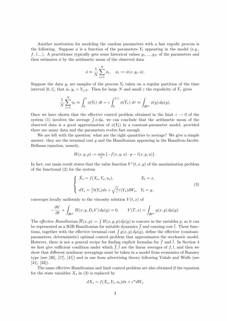
Another motivation for modeling the random parameters with a fast ergodic process isthe following. Suppose φ is a function of the parameters Yt appearing in the model (e.g.,f , l....). A practitioner typically gets some historical values y1, ..., yN of the parameters andthen estimates φ by the arithmetic mean of the observed data

φ ≈ 1N

N∑i=1

φi, φi := φ(x, yi, u).

Suppose the data yi are samples of the process Yt taken on a regular partition of the timeinterval [0, 1], that is, yi = Yi/N . Then for large N and small ε the ergodicity of Yτ gives

1N

N∑i=1

φi ≈∫ 1

0φ(Yt) dt = ε

∫ 1/ε

0φ(Yτ ) dτ ≈

∫IRm

φ(y) dµ(y).

Once we have shown that the effective control problem obtained in the limit ε → 0 of thesystem (1) involves the average

∫φdµ, we can conclude that the arithmetic mean of the

observed data is a good approximation of φ(Yt) in a constant-parameter model, providedthere are many data and the parameters evolve fast enough.

We are left with the question: what are the right quantities to average? We give a simpleanswer: they are the terminal cost g and the Hamiltonian appearing in the Hamilton-Jacobi-Bellman equation, namely,

H(x, y, p) := minu−f(x, y, u) · p− l(x, y, u) .

In fact, our main result states that the value function V ε(t, x, y) of the maximization problemof the functional (2) for the system

Xs = f(Xs, Ys, us), Xt = x,

dYs = 1εb(Ys)ds+

√2ετ(Ys)dWs, Yt = y,

(3)

converges locally uniformly to the viscosity solution V (t, x) of

−∂V∂t

+∫

IRm

H(x, y,DxV ) dµ(y) = 0, V (T, x) =∫

IRm

g(x, y) dµ(y).

The effective Hamiltonian H(x, p) :=∫H(x, y, p) dµ(y) is concave in the variables p, so it can

be represented as a HJB Hamiltonian for suitable dynamics f and running cost l. These func-tions, together with the effective terminal cost

∫g(x, y) dµ(y), define the effective (constant-

parameters, deterministic) optimal control problem that approximates the stochastic model.However, there is not a general recipe for finding explicit formulas for f and l. In Section 4we first give sufficient condition under which f, l are the linear averages of f, l, and then weshow that different nonlinear averagings must be taken in a model from economics of Ramseytype (see [30], [17], [41]) and in one from advertising theory following Vidale and Wolfe (see[41], [33]).

The same effective Hamiltonian and limit control problem are also obtained if the equationfor the state variables Xs in (3) is replaced by

dXs = f(Xs, Ys, us)ds+ εαdWs

3

for some α > 0. Therefore the effective control problem is the same if the dynamics is alsoaffected by a small white noise, in addition to the fast oscillating stochastic parameters.

Our method is based on the HJB equation and uses the theory of viscosity solutions (see[6] and [20]). It allows us to treat a more general problem than (3), namely

dXt = f(Xt, Yt, ut)dt+√

2σε(Xt, Yt, ut)dWt Xto = x ∈ IRn,

dYt = 1εb(Xt, Yt)dt+

√2ετ(Xt, Yt)dWt Yto = y ∈ IRm,

(4)

with σε → σ locally uniformly. Here the evolution of the Xs variables is disturbed by a whitenoise and the matrices σε, σ satisfy only standard regularity and growth assumptions and canbe degenerate, so that the previous cases are recovered by taking σ ≡ 0 and either σε ≡ 0 orσε = εαI. Moreover, the evolution of the Ys variables is now no more decoupled, thereforedescribing the case when the parameters are influenced by the state Xs. This generalityapplies also to models where Ys are not parameters but true state variables that evolve on afaster time scale than Xs, provided they are uncontrolled.

Our results fall within the domain of singular perturbations of diffusion processes andof control systems. There is a wide literature on this subject and its applications, see therecent survey papers [22, 38] and their large bibliographies. For results based on probabilisticmethods we refer to the books [35, 34], the recent papers [39, 40, 13, 14], and the referencestherein. An approach based on the HJB equations started with [32, 10] and was developedwithin the theory of viscosity solutions by Alvarez and one of the authors in [1, 2, 3], seealso [4, 5] for problems with an arbitrary number of scales. These methods originate inperiodic homogenization theory [37, 24] and work nicely for fast variables restricted to acompact set, in particular the m-dimensional torus. The contribution of this paper is thetreatment of unbounded fast variables Yt, such as the classical Ornstein-Uhlenbeck process.In the companion paper [7] similar results were given for financial models with stochasticvolatility, that have a special structure, null running cost, and dynamics of the fast variablesindependent of Xs. We use here some ergodic results of [7]. A convergence theorem in theunbounded setting was proved by Kushner [35] with probabilistic methods in the case of fastvariables and controls appearing in a decoupled way, so that the effective system and cost arethe linear averages of f and l. We get a variant of his theorem as a special case of ours inSection 4.1. Our results are also related to the theory of well-posedness of control problems[23] and to sensitivity analysis in optimization [18, 43, 12].

Finally let us mention that a different model of stochastic control problems with fastrandom oscillations was studied by Bensoussan and Blankenship [11]. It fits in the recenttheory of homogenization of fully nonlinear elliptic PDEs in stationary ergodic media [16].

The paper is organized as follows. Section 2 presents the mathematical problem withthe precise assumptions, the HJB equation, and the initial value problem satisfied by V ε.In Section 3 we construct the effective Hamiltonian and terminal cost and prove the mainresult, Theorem 3.2, on the convergence of V ε to the solution of the effective Cauchy problem.Section 4 is devoted to examples and applications. For the economic model of Section 4.2 wealso discuss the convergence of the optimal feedback control for the problem with ε > 0 tothe one for the effective problem.

4

2 The two-scale stochastic control problem

2.1 The stochastic system

Let (Ω,F ,Ft,P) be a complete filtered probability space and let (Wt)t be an Ft-adaptedstandard r-dimensional Brownian motion. We consider the stochastic control system (4)where ε > 0 and the coefficients satisfy the following standard conditions. We will usethe symbols Mk,j and Sk to denote, respectively, the set of k × j matrices and the set ofk × k symmetric matrices. For a given compact set U , f : IRn × IRm × U → IRn andσε : IRn × IRm ×U → Mn,r are continuous functions, Lipschitz continuous in (x, y) uniformlyw.r.t. u ∈ U and ε > 0 and with linear growth in x, i.e.

for some C > 0 |f(x, y, u)|, ‖σε(x, y, u)‖ ≤ C(1 + |x|) ∀x, y, ∀ε > 0. (5)

Moreover we assume that

limε→0

σε(x, y, u) = σ(x, y, u) locally uniformly,

where σ : IRn × IRm × U → Mn,r satisfies the same conditions as σε. The coefficientsb : IRn × IRm → IRm and τ : IRn × IRm → Mm,r are locally Lipschitz continuous functionswith linear growth, i.e.

for some C > 0 |b(x, y)|, ‖τ(x, y)‖ ≤ C(1 + |x|+ |y|) for every x, y. (6)

Finally, the diffusion driving the fast variables Yt is uniformly non degenerate, i.e.,

∃Λ(y) > 0 such that ξτ(x, y)τT (x, y) · ξ = |ξτ(x, y)|2 ≥ Λ(y)|ξ|2 ∀x, y, ξ. (7)

We will not make any non-degeneracy assumption on the matrices σε, σ, so the case σ ≡ 0 isallowed.

2.2 The optimal control problem

We define the following pay off functional for a finite horizon optimal control problem asso-ciated to system (4)

J(t, x, y, u) := E[eλ(t−T )g(XT , YT ) +

∫ T

tl(Xs, Ys, us)eλ(s−T )ds | Xt = x, Yt = y

], t ∈ [0, T ],

where E denotes the conditional expectation. The associated value function is

V ε(t, x, y) := supu·∈U

J(t, x, y, u).

The discount factor is λ ≥ 0. The utility function g : IRn × IRm → IR and the running costl : IRn × IRm × U → IR are continuous functions and satisfy

∃K > 0 such that supy∈IRm

|g(x, y)|, supy∈IRm,u∈U

|l(x, y, u)| ≤ K(1 + |x|2) ∀x ∈ IRn. (8)

The set of admissible control functions U is the standard one in stochastic control problems(see [25, Ch. IV, Definition 2]), i.e. it is the set of Ft−progressively measurable processestaking values in U .

These conditions and those of the preceding Section will hold throughout the paper.

5

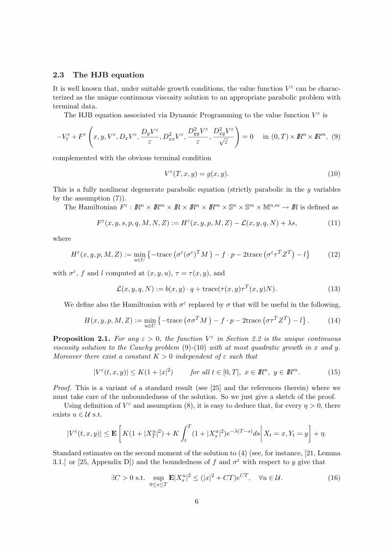
2.3 The HJB equation

It is well known that, under suitable growth conditions, the value function V ε can be charac-terized as the unique continuous viscosity solution to an appropriate parabolic problem withterminal data.

The HJB equation associated via Dynamic Programming to the value function V ε is

−V εt +F ε

(x, y, V ε, DxV

ε,DyV

ε

ε,D2

xxVε,D2

yyVε

ε,D2

xyVε

√ε

)= 0 in (0, T )× IRn× IRm, (9)

complemented with the obvious terminal condition

V ε(T, x, y) = g(x, y). (10)

This is a fully nonlinear degenerate parabolic equation (strictly parabolic in the y variablesby the assumption (7)).

The Hamiltonian F ε : IRn × IRm × IR× IRn × IRm × Sn × Sm ×Mn,m → IR is defined as

F ε(x, y, s, p, q,M,N,Z) := Hε(x, y, p,M,Z)− L(x, y, q,N) + λs, (11)

where

Hε(x, y, p,M,Z) := minu∈U

−trace

(σε(σε)TM

)− f · p− 2trace

(σετTZT

)− l

(12)

with σε, f and l computed at (x, y, u), τ = τ(x, y), and

L(x, y, q,N) := b(x, y) · q + trace(τ(x, y)τT (x, y)N). (13)

We define also the Hamiltonian with σε replaced by σ that will be useful in the following,

H(x, y, p,M,Z) := minu∈U

−trace

(σσTM

)− f · p− 2trace

(στTZT

)− l. (14)

Proposition 2.1. For any ε > 0, the function V ε in Section 2.2 is the unique continuousviscosity solution to the Cauchy problem (9)-(10) with at most quadratic growth in x and y.Moreover there exist a constant K > 0 independent of ε such that

|V ε(t, x, y)| ≤ K(1 + |x|2) for all t ∈ [0, T ], x ∈ IRn, y ∈ IRm. (15)

Proof. This is a variant of a standard result (see [25] and the references therein) where wemust take care of the unboundedness of the solution. So we just give a sketch of the proof.

Using definition of V ε and assumption (8), it is easy to deduce that, for every η > 0, thereexists u ∈ U s.t.

|V ε(t, x, y)| ≤ E[K(1 + |Xu

T |2) +K

∫ T

t(1 + |Xu

s |2)e−λ(T−s)ds

∣∣∣∣Xt = x, Yt = y

]+ η.

Standard estimates on the second moment of the solution to (4) (see, for instance, [21, Lemma3.1.] or [25, Appendix D]) and the boundedness of f and σε with respect to y give that

∃C > 0 s.t. sup0≤s≤T

E|Xus |2 ≤ (|x|2 + CT )eCT , ∀u ∈ U . (16)

6

From this we get immediately (15) and this estimate in particular implies that the functionsV ε are locally equibounded.

We define the lower and upper semicontinuous envelope of V ε as

V ε∗ (t, x, y) = lim inf

(t′,x′,y′)→(t,x,y)V ε(t′, x′, y′) and (V ε)∗(t, x, y) = lim sup

(t′,x′,y′)→(t,x,y)V ε(t′, x′, y′).

By definition V ε∗ (t, x, y) ≤ V ε(t, x, y) ≤ (V ε)∗(t, x, y). A standard argument in viscosity

solution theory, based on the dynamic programming principle (see, e.g., [25, Ch. IV, Thm7.1], [15, Thm 4.1]), gives that V ε

∗ and (V ε)∗ are, respectively, a viscosity supersolution anda viscosity subsolution to (9), at every point (t, x, y) ∈ (0, T )× IRn × IRm.

Moreover limt→T Vε(t, x, y) = g(x, y) locally uniformly in (x, y) ∈ IRn×IRm. This result is

well known and follows from (8), (16), and from the continuity in mean square of Xt, Yt. Forexample, the same argument detailed in the proof of Proposition 3.1 in [7] can be repeatedwith minor changes.

Then the conclusion is obtained using a recent comparison result between sub and super-solutions to parabolic problems satisfying the quadratic growth condition

|V (t, x, y)| ≤ K(1 + |x|2 + |y|2)

proved in Theorem 2.1 in [21]. Since V ε satisfies (15) the result applies in our case, so(V ε)∗(t, x, y) ≤ V ε

∗ (t, x, y). Recalling the definition of semicontinuous envelopes, we get

(V ε)∗(t, x, y) = V ε∗ (t, x, y) = V ε(t, x, y) ∀ (t, x, y) ∈ [0, T ]× IRn × IRm.

This implies that V ε is a continuous viscosity solutions of (9), and, again by Theorem 2.1 in[21], that it is the unique solution with at most quadratic growth in x and y.

2.4 Ergodicity of the fast variables

Consider the diffusion processes in IRm obtained putting ε = 1 in (4) and fixing x ∈ IRn

dYt = b(x, Yt)dt+√

2τ(x, Yt)dWt, (17)

called the fast subsystems. To recall the dependance on the parameter x, we will denote theprocess in (17) as Y x

· . Observe that its infinitesimal generator is Lxw := L(x, y,Dyw,D2yyw),

with L defined by (13) .Throughout the paper, we will assume the following condition:

∀x ∈ IRn there exists w ∈ C(IRm), k > 0, R0 > 0 such that

−Lxw ≥ k for |y| > R0 in viscosity sense , and w(y) → +∞ as |y| → +∞. (18)

This condition is reminiscent of other similar conditions about ergodicity of diffusionprocesses in the whole space, see for example [29], [10], [36], [14], [13]. Lions and Musiela [36]also state that (18) is indeed equivalent to the ergodicity of the process in (17) and to theclassical Lyapunov-type condition of Hasminskii [29].

Remark 2.1. Condition (18) can be interpreted as a weak Lyapunov condition for the process(17) relative to the set |y| ≤ R0. Indeed, a Lyapunov function for the system (17) relativeto a compact invariant set K is a continuous, positive definite function L such that L(y) = 0if and only if y ∈ K, the sublevel sets y |L(y) ≤ k are compact and −LxL(y) = l(y) in IRm,where l is a continuous function with l = 0 on K and l > 0 outside. For more details see [29].

7

Example 2.1. Condition (18) is satisfied if, for every x ∈ IRn,

lim sup|y|→+∞

[b(x, y) · y + trace(τ(x, y)τT (x, y))

]< 0.

In this case it is immediate to check (18) by choosing w(y) = |y|2 and R0 sufficiently big. Atypical model process which satisfies the previous condition is the Ornstein-Uhlenbeck processwith equation

dYt = (m(x)− Yt)dt+√

2τ(x)dWt.

Pardoux and Veretennikov [39, 40] assume ττT bounded and lim|y|→+∞ supx b(x, y) ·y = −∞,and call it recurrence condition.

In the following we give two results from [7] saying that, under (18) and the standingassumptions in Section 2.1, the process Y x

· in (17) is ergodic, in the sense that it has a uniqueinvariant measure, and a Liouville property holds. Moreover, we will discuss the regularityof the invariant measure w.r.t. the frozen variable x. The Liouville property replaces thestandard strong maximum principle of the periodic case and is the key ingredient for extendingsome results of [3] to the non-periodic setting. The proof is in [7], Lemma 4.1.

Lemma 2.1. For x ∈ IRn fixed, consider the problem

−LxV = −L(x, y,DV (y), D2V (y)) = 0 y ∈ IRm. (19)

Then

i) every bounded viscosity subsolution to (19) is constant;

ii) every bounded viscosity supersolution to (19) is constant.

Next we state the existence and uniqueness of an invariant measure, see Proposition 4.2in [7] (see also chapter IV in [29]).

Proposition 2.2. Under the standing assumptions, for every x ∈ IRn, there exists a uniqueinvariant probability measure µx on IRm for the process Y x

· .

Example 2.2. For the multi-dimensional Ornstein-Uhlenbeck process

dYt = (m(x)− Yt)dt+√

2τ(x)dWt.

the invariant measure has the explicit expression (see e.g. Section 4.1.2 in [19], see also Section3.2.3 in [26])

dµx(y) =1

(2π)m/2 det(ττT (x))exp

[−1

2(ττT (x))−1(y −m(x)) · (y −m(x))

]dy ∀x.

Finally, the last result is about the Lipschitz regularity of µx with respect to x. This resultwill be a key ingredient to prove locally Lipschitz regularity in x of the effective Hamiltonian(24). Obviously, when b, τ do not depend on x this regularity property is trivially satisfied.

8

Proposition 2.3. Besides the standing assumptions, assume that

b ∈ C1(IRn × IRm, IRm) and τ ∈ C1(IRn × IRm,Mm,r) (20)

with all their derivatives bounded and Holder continuous in y uniformly in x. Then theinvariant measure µx of the process Y x

· has a density ϕx(y) and there exist k > 1, C > 0,such that

|ϕx1(y)− ϕx2(y)| ≤ C1

1 + |y|k|x1 − x2|, ∀x1, x2 ∈ IRn, y ∈ IRm.

Proof. For the proof we refer to Theorem 6 in [40], where such result is proved by PDEmethods. The idea is to consider the adjoint operator to Lx and to study the dependenceof the solutions of the adjoint equation on the parameter x. The main tools are non trivialestimates on the fundamental solutions of nondegenerate second order parabolic PDEs.

Remark 2.2. In [13] there is an analogous result (Prop. 5.2) about the Lipschitz regularityw.r.t. x of the effective system obtained by the average of a singularly perturbed stochasticsystem such as (4), under different assumptions and using mainly stochastic control methods.The authors replace regularity conditions such as (20) with appropriate estimates on thetrajectories of the system, such as:

∃C > 0 s.t. E|Y x1t − Y x2

t | ≤ C|x1 − x2| ∀t ≥ 0

where Y xi· is the process in (17) with x = xi and Y0 = y. The authors state that this estimatecan be obtained by an exponential stability condition on the process Y such as

∃a, b > 0 s.t. E|(Y ′)xt − (Y ′′)x

t | ≤ ae−bt|y′ − y′′|, ∀t ≥ 0, ∀x,

where (Y ′)x· and (Y ′′)x

· both satisfy (17) with initial condition respectively (Y ′)x0 = y′ and

(Y ′′)x0 = y′′.

3 The convergence result

This section is devoted to the main result of the paper, namely, the convergence theorem forthe singular perturbation problem. First of all, we will construct the effective Hamiltonian Hand the effective terminal data g. Then we will prove in Theorem 3.2 that the value functionV ε(t, x, y), solution to (9), converges locally uniformly, as ε→ 0, to a function V (t, x) whichwill be characterized as the unique solution of the Cauchy problem

−Vt +H(x,DxV,D

2xxV

)+ λV (x) = 0 in (0, T )× IRn

V (T, x) = g(x) in IRn.(21)

3.1 The effective Hamiltonian and initial data

Section 2.4 contains the main tools to define the candidate limit Cauchy problem of thesingularly perturbed problem (9) as ε → 0. We start showing the existence of an effective

9

Hamiltonian giving the limit PDE. In principle, for each (x, p, P ) one expects the effectiveHamiltonian H(x, p, P ) to be the unique constant c ∈ IR such that the cell problem

−L(x, y,Dχ,D2χ) +H(x, y, p, P , 0) = c in IRm, (22)

where H is defined in (14), has a viscosity solution χ, called corrector (see [37], [24], [1]).Actually, for our approach, it is sufficient to consider, as in [2], a δ-cell problem

δwδ − L(x, y,Dwδ, D2wδ) +H(x, y, p, P , 0) = 0 in IRm, (23)

whose solution wδ is called approximate corrector. The next result states that δwδ convergesto −H and it is smooth.

Theorem 3.1. Under the standing assumptions in Sections 2.1, 2.2 and 2.4, for any fixed(x, p, P ) and δ > 0 there exists a solution wδ = wδ;x,p,P (y) in C2(IRm) of (23) such that

− limδ→0

δwδ = H(x, p, P ) :=∫

IRm

H(x, y, p, P , 0) dµx(y) locally uniformly in IRm, (24)

where µx is the invariant probability measure on IRm for the process Y x· .

The proof is given in [7], Theorem 4.3.We define now the effective terminal value for the limit as ε → 0 of the singular pertur-

bation problem (9). We fix x and consider the following Cauchy initial problem:wt − L(x, y,Dw,D2w) = 0 in (0,+∞)× IRm

w(0, y) = g(x, y),(25)

where g satisfies assumption (8).

Proposition 3.1. Under the standing assumptions in Sections 2.1, 2.2 and 2.4, for every xthere exists a unique bounded classical solution w(·, ·;x) to (25) and

limt→+∞

w(t, y;x) =∫

IRm

g(x, y)dµx(y) =: g(x) locally uniformly in y. (26)

Moreover g is continuous and satisfy a quadratic growth condition as (8).

Proof. The proof can be found in [7] Proposition 4.4. The regularity of g and the growthcondition can be obtained, using the definition of g, from condition (8) and the regularity ofthe invariant measure stated in Proposition 2.3.

We say that the Comparison Principle holds for a Cauchy problem as (21) ifgiven U ∈ USC([0, T ] × IRn) and V ∈ LSC([0, T ] × IRn), respectively, a subsolution and asupersolution to the PDE and such that

U(T, x) ≤ V (T, x) for every x,∃C > 0 s.t. |U(t, x)|, |V (t, x)| ≤ C(1 + |x|2) for every t, x,

then U(t, x) ≤ V (t, x) in [0, T ]× IRn.

10

Proposition 3.2. Under the standing assumptions in Sections 2.1, 2.2 and 2.4, the Com-parison Principle holds for the effective Cauchy problem (21) with H and g given by (24) and(26) if at least one of the following five sets of assumptions is verified:

(i) b, τ are independent of x;

(ii) σε → σ ≡ 0 and b, τ satisfy the regularity assumptions (20);

(iii) the fast subsystem is Ornstein-Uhlenbeck, i.e., b(x, y) = m(x) − y and τ(x, y) = τ(x),with m ∈ C1(IRn, IRm), τ ∈ C1(IRn,Mm,r), and τ(x)τT (x) ≥ τ0I with τ0 > 0;

(iv) σε → σ(x, u) (independent of y) and b, τ satisfy the regularity assumptions (20);

(v) σε → σ(x, y) (independent of u), there exists a Lipschitz σ : IRn → Mn,r such that

σ(x)σ(x)T =∫

IRm

σ(x, y)σT (x, y) dµx(y),

f and l are bounded, b, τ satisfy the regularity assumptions (20), for some C > 0 gsatisfies

|g(x1, y)− g(x2, y)| ≤ C(1 + |x1|+ |x2|)|x1 − x2| ∀x1, x2, y,

and either g is independent of y, or it has at most linear growth in x:

|g(x, y)| ≤ C(1 + |x|).

Proof. In the case (i) the effective Hamiltonian is the average with respect to a measure µ(y)of a Hamiltonian satisfying the structural assumptions of [21] for the Comparison Principle,uniformly in y. It is immediate to check that the same proof as in [21, Thm 2.1] holds for theCauchy problem with averaged Hamiltonian as well. Similarly, it is easy to check that thesame arguments work also in case (iv). Finally, also in case (iii) the Comparison Principlecan be obtained following the proof of [21, Thm 2.1]. Indeed the main point in this case is tocheck that for every R > 0 there exists some CR > 0 such that, for every u ∈ U ,∫

IRm

∣∣∣σ(x1, y, u)√ϕx1(y)− σ(x2, y, u)

√ϕx2(y)

∣∣∣2 dy ≤ CR|x1 − x2|2, ∀x1, x2 ∈ B(0, R).

This is satisfied when, e.g.,∫IRm

|Dxϕx(y)|2

ϕx(y)dy ≤ CR, ∀x ∈ B(0, R).

This is the case of the Ornstein-Uhlenbeck process under the assumptions in (iii), as it ispossible to check with straightforward computations on the explicit formula given in Example2.2.

Case (ii) is actually a particular case of (iv), but we state it separately because theeffective Hamiltonian H is of the first order and so the proof is much easier. Using thestanding assumptions and Proposition 2.3 one checks that H satisfies the following structuralconditions: there exists C > 0 such that

|H(x, p1)−H(x, p2)| ≤ C(1 + |x|)|p1 − p2|, ∀x, p1, p2 ∈ IRn, (27)

11

and for every R > 0 there exists a continuity modulus ωR s.t.

|H(x1, p)−H(x2, p)| ≤ ωR(|x1 − x2|(1 + |p|)), ∀x1, x2 ∈ B(0, R), p ∈ IRn. (28)

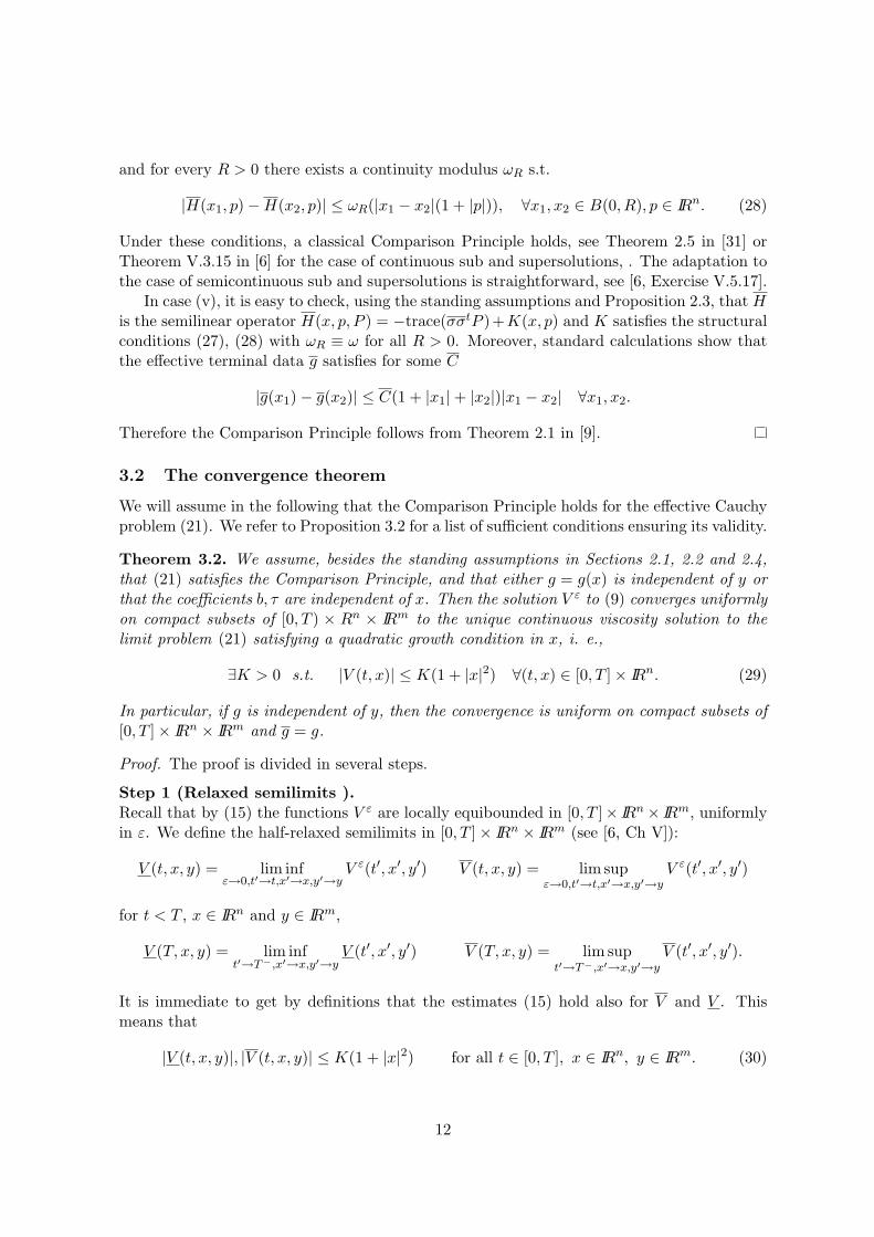
Under these conditions, a classical Comparison Principle holds, see Theorem 2.5 in [31] orTheorem V.3.15 in [6] for the case of continuous sub and supersolutions, . The adaptation tothe case of semicontinuous sub and supersolutions is straightforward, see [6, Exercise V.5.17].

In case (v), it is easy to check, using the standing assumptions and Proposition 2.3, that His the semilinear operator H(x, p, P ) = −trace(σσtP )+K(x, p) and K satisfies the structuralconditions (27), (28) with ωR ≡ ω for all R > 0. Moreover, standard calculations show thatthe effective terminal data g satisfies for some C

|g(x1)− g(x2)| ≤ C(1 + |x1|+ |x2|)|x1 − x2| ∀x1, x2.

Therefore the Comparison Principle follows from Theorem 2.1 in [9].

3.2 The convergence theorem

We will assume in the following that the Comparison Principle holds for the effective Cauchyproblem (21). We refer to Proposition 3.2 for a list of sufficient conditions ensuring its validity.

Theorem 3.2. We assume, besides the standing assumptions in Sections 2.1, 2.2 and 2.4,that (21) satisfies the Comparison Principle, and that either g = g(x) is independent of y orthat the coefficients b, τ are independent of x. Then the solution V ε to (9) converges uniformlyon compact subsets of [0, T ) × Rn × IRm to the unique continuous viscosity solution to thelimit problem (21) satisfying a quadratic growth condition in x, i. e.,

∃K > 0 s.t. |V (t, x)| ≤ K(1 + |x|2) ∀(t, x) ∈ [0, T ]× IRn. (29)

In particular, if g is independent of y, then the convergence is uniform on compact subsets of[0, T ]× IRn × IRm and g = g.

Proof. The proof is divided in several steps.

Step 1 (Relaxed semilimits ).Recall that by (15) the functions V ε are locally equibounded in [0, T ]× IRn × IRm, uniformlyin ε. We define the half-relaxed semilimits in [0, T ]× IRn × IRm (see [6, Ch V]):

V (t, x, y) = lim infε→0,t′→t,x′→x,y′→y

V ε(t′, x′, y′) V (t, x, y) = lim supε→0,t′→t,x′→x,y′→y

V ε(t′, x′, y′)

for t < T , x ∈ IRn and y ∈ IRm,

V (T, x, y) = lim inft′→T−,x′→x,y′→y

V (t′, x′, y′) V (T, x, y) = lim supt′→T−,x′→x,y′→y

V (t′, x′, y′).

It is immediate to get by definitions that the estimates (15) hold also for V and V . Thismeans that

|V (t, x, y)|, |V (t, x, y)| ≤ K(1 + |x|2) for all t ∈ [0, T ], x ∈ IRn, y ∈ IRm. (30)

12

Step 2 (V , V do not depend on y).We check that V (t, x, y), V (t, x, y) do not depend on y, for every t ∈ [0, T ) and x ∈ IRn.We claim that V (t, x, y) (resp., V (t, x, y)) is, for every t ∈ (0, T ) and x ∈ IRn, a viscositysubsolution (resp., supersolution) to

−L(x, y,DyV,D2yyV ) = 0 in IRm (31)

where L is the differential operator defined in (13). If the claim is true, we can use Lemma2.1, since V , V are bounded in y according to estimates (30), to conclude that the functionsy → V (t, x, y), y → V (t, x, y) are constants for every (t, x) ∈ (0, T )× IRn. Finally, using thedefinition it is immediate to see that this implies that also V (T, x, y) and V (T, x, y) do notdepend on y. We prove the claim only for V , since the other case is completely analogous.

First of all we show that the function V (t, x, y) is a viscosity subsolution to (31). To dothis, we fix a point (t, x, y) and a smooth function ψ such that V −ψ has a maximum at (t, x, y)in B = B((t, x, y), r), for some fixed r > 0. Using the definition of weak relaxed semilimits itis possible to prove (see [6, Lemma V.1.6]) that there exists εn → 0 and B 3 (tn, xn, yn) →(t, x, y) maxima for V εn − ψ in B such that V εn(tn, xn, yn) → V (t, x, y). Therefore, recallingthat V ε is a subsolution to (9), we get

−ψt +H

(xn, yn, Dxψ,D

2xxψ,

1√εnD2

xyψ

)− 1εnL(xn, yn, Dyψ,D

2yyψ) + λV εn(tn, xn, yn) ≤ 0,

where all the derivatives of ψ are computed resp. in (tn, xn, yn). This implies

−L(xn, yn, Dyψ,D2yyψ) ≤ εn

[ψt −H

(xn, yn, Dxψ,D

2xxψ,

1√εnD2

xyψ

)− λV εn(tn, xn, yn)

].

We observe that the part between brackets in the right-hand side of the previous is uniformlybounded with respect to n in B and using the regularity properties of ψ and of the coefficientsin the equation we get, as εn → 0, the desired conclusion.

We show now that if V (t, x, y) is a subsolution to (31), then for every fixed (t, x) thefunction y 7→ V (t, x, y) is a subsolution to (31), which was our claim. To do this, we fix y anda smooth function φ such that V (t, x, ·)−φ has a strict local maximum at y in B(y, δ) and suchthat φ(y) ≥ 1 for all y ∈ B(y, δ). We define, for η > 0, φη(t, x, y) = φ(y)

(1 + |x−x|2+|t−t|2

η

)and we consider (tη, xη, yη) a maximum point of V −φη in B((t, x, y), δ). Repeating the sameargument as in [6, Lemma II.5.17], it is possible to prove, eventually passing to subsequences,that, as η → 0, (tη, xη, yη) → (t, x, y) and Kη :=

(1 + |xη−x|2+|tη−t|2

η

)→ K > 0. Moreover,

using the fact that V is a subsolution to (31), we get −L(xη, yη,KηDφ(yη),KηD2φ(yη) ≤ 0,

which gives, using the linearity of L and passing to the limit as η → 0, the desired conclusion−L(x, y,Dφ(y), D2φ(y)) ≤ 0.

Step 3 (V and V are sub and supersolutions of the limit PDE).First we claim that V and V are sub and supersolution to the PDE in (21) in (0, T ) × IRn.We prove the claim only for V since the other case is completely analogous. The proofadapts the perturbed test function method introduced in [24] for the periodic setting. Wefix (t, x) ∈ ((0, T ) × IRn) and we show that V is a viscosity subsolution at (t, x) of the limitproblem. This means that if ψ is a smooth function such that ψ(t, x) = V (t, x) and V − ψhas a maximum at (t, x) then

−ψt(t, x) +H(x,Dxψ(t, x), D2xxψ(t, x)) + λV (t, x) ≤ 0. (32)

13

Without loss of generality we assume that the maximum is strict in B((t, x), r) and that0 < t − r < t + r < T . We fix y ∈ IRm, η > 0 and consider a solution χ = wδ ∈ C2 of theδ-cell problem (23) at (x,Dxψ(t, x), D2

xxψ(t, x)) (see Theorem 3.1) such that

|δχ(y) +H(x,Dxψ(t, x), D2xxψ(t, x))| ≤ η ∀ y ∈ B(y, r). (33)

We define the perturbed test function as

ψε(t, x, y) := ψ(t, x) + εχ(y).

Observe that

lim supε→0,t′→t,x′→x,y′→y

V ε(t′, x′, y′)− ψε(t′, x′, y′) = V (t, x)− ψ(t, x).

By a standard argument in viscosity solution theory (see [6, Lemma V.1.6], [20]) we get thatthere exist sequences εn → 0 and (tn, xn, yn) ∈ B := B((t, x, y), r) such that:

(tn, xn, yn) → (t, x, y), for some y ∈ B(y, r),

V εn(tn, xn, yn)− ψεn(tn, xn, yn) → V (t, x)− ψ(t, x),

(tn, xn, yn) is a strict maximum of V εn − ψεn in B.

Then, using the fact that V ε is a subsolution to (9), we get

−ψt +Hεn(xn, yn, Dxψ,D

2xxψ, 0

)+ λV εn(tn, xn, yn)− L(xn, yn, Dyχ,D

2yyχ) ≤ 0 (34)

where the derivatives of ψ and χ are computed respectively in (tn, xn) and in yn. Using thefact that χ solves the δ-cell problem (23), we obtain

−ψt(tn, xn)− δχ(yn) + λV εn(tn, xn, yn) ≤≤ H(x, yn, Dxψ(t, x), D2

xxψ(t, x), 0)−Hεn(xn, yn, Dxψ(tn, xn), D2xxψ(tn, xn), 0)

+ L(xn, yn, Dyχ,D2yyχ)− L(x, yn, Dyχ,D

2yyχ).

By taking the limit as n→ +∞ the r.h.s. of this inequality cancel out. Next we use (33) toreplace −δχ with H − η and get that the left hand side of (32) is ≤ η. Finally, by lettingη → 0 we obtain (32).

Step 4 (Behaviour of V and V at time T ).We show that, at every x, V (x, T ) ≤ g(x) and V (x, T ) ≥ g(x).

We start with V . If g = g(x, y) and the coefficients b, τ are independent of x, we reproduceand complete the argument given in [7, Thm 5.1, Step 4]. We fix x ∈ IRn and denote wr theunique bounded classical solution to

wt − L(y,Dw,D2w) = 0 in (0,+∞)× IRm

wr(0, y) = sup|x−x|≤r g(x, y) in IRm.(35)

By Proposition 3.1, limt→+∞wr(t, y) =∫IRm sup|x−x|≤r g(x, y)dµ(y) =: gr(x) locally uni-

formly in y, where µ is the invariant probability measure on IRm for the process Y . Note thatsup|x−x|≤r1

g(x, y) ≥ sup|x−x|≤r2g(x, y) for r1 ≥ r2 ≥ 0, y ∈ IRm and limr→0 sup|x−x|≤r g(x, y) =

g(x, y). So, by monotone convergence theorem, limr→0 gr(x) = g(x).

14

We fix r > 0 and a constant Kr > 0 such that V ε(t, x, y) ≤ Kr and |g(x, y)| ≤ Kr/2 forevery ε > 0, x ∈ Br := B(x, r), y ∈ IRm and t ∈ [0, T ]. Observe that this is possible byestimates (15) and assumption (8). Moreover we fix a smooth nonnegative function ψr suchthat ψr(x) = 0 and ψr(x)+infy g(x, y) ≥ Kr for every x ∈ ∂Br. Let Cr be a positive constantsuch that

|Hε(x, y,Dψr(x), D2ψr(x), 0)| ≤ Cr for x ∈ Br, y ∈ IRm and ε > 0

where Hε is defined in (12). Note that such constant exists due to assumptions (5) and (8).We define the function

ψεr(t, x, y) = wr

(T − t

ε, y

)+ ψr(x) + Cr(T − t)

and we claim that it is a supersolution to the parabolic problem−Vt + F ε

(x, y, V,DxV,

DyVε , D2

xxV,D2

yyV

ε ,D2

xyV√ε

)= 0 in (0, T )×Br × IRm

V (t, x, y) = Kr in (0, T )× ∂Br × IRm

V (T, x, y) = g(x, y) in Br × IRm

(36)

where F ε is defined in (11). Indeed

−(ψεr)t + F ε

(x, y,Dxψ

εr ,Dyψ

εr

ε,D2

xxψεr ,D2

yyψεr

ε,D2

xyψεr√

ε

)=

=1ε

[(wr)t − L(y,Dwr, D

2wr)]+ Cr +Hε(y, x,Dψr(x), D2ψr(x), 0) ≥ 0.

Moreover ψεr(T, x, y) = sup|x−x|≤r g(x, y) + ψr(x) ≥ g(x, y). Finally, observe that the con-

stant function infy sup|x−x|≤r g(x, y) is always a subsolution to (35) and then by a standardcomparison principle we obtain wr(t, y) ≥ infy sup|x−x|≤r g(x, y). This implies

ψεr(t, x, y) ≥ inf

ysup

|x−x|≤rg(x, y) +Kr − inf

yg(x, y) + Cr(T − t) ≥ Kr ∀ x ∈ ∂Br.

Then ψε is a supersolution to (36). For our choice of Kr, we get that V ε is a subsolution to(36). Moreover both V ε and ψε

r are bounded in [0, T ]×Br×IRm, because of the estimate (15),of the boundedness of wr and of the regularity of ψr. So, a standard comparison principle forviscosity solutions gives

V ε(t, x, y) ≤ ψεr(t, x, y) = wr

(T − t

ε, y

)+ ψr(x) + Cr(T − t)

for every r > 0, ε > 0, (t, x, y) ∈ ([0, T ] × Br × IRm). We compute the upper limit of bothsides of the previous inequality as (ε, t, x, y) → (0, t′, x′, y′) for t′ ∈ (0, T ), x′ ∈ Br, y′ ∈ IRm

and getV (t′, x′) ≤ gr(x) + ψr(x′) + Cr(T − t′).

Then, taking the upper limit for (t′, x′) → (T, x), we obtain V (T, x) ≤ gr(x), for every r > 0.This permits to conclude, sending r → 0.

If g does not depend on y, we get that the function ψεr(t, x, y) = sup|x−x|≤r g(x)+ψr(x)+

Cr(T − t) is a supersolution to (36), and the conclusion easily follows.

15

The proof for V is completely analogous, once we replace the Cauchy problem (35) withwt − L(y,Dw,D2w) = 0 in (0,+∞)× IRm

w(0, y) = inf|x−x|≤r g(x, y) in IRm.

Step 5 (Uniform convergence).Observe that both V and V satisfy the same quadratic growth condition (30). Moreover weassume that the Comparison Principle holds for the problem (21), so V ≥ V . Therefore, sinceby definition V ≤ V , we conclude V = V =: V . This implies that V is continuous and that,by the definition of semilimits, V ε converges loc. uniformly to V (see [6, Lemma V.1.9]).

4 Examples and applications

In this section we look for a control problem whose value function is the limit V of the valuefunctions V ε. It is enough to represent the effective Hamiltonian H as a HJB Hamiltonian,that is,

H(x, p, P ) = minu∈U

−trace(σσT (x, u)P )− f(x, u) · p− l(x, u)

, (37)

for some compact set U and continuous f, σ, l, with f, σ Lipschitz in x. Indeed in this casethe uniqueness of the viscosity solution to the Cauchy problem for HJB equations gives theformula

V (t, x) := supu.

E[∫ T

tl(Xs, us)ds+ 〈g〉(XT )

],

for Xs solvingdXs = f(Xs, us)ds+

√2σ(Xs, us)dWs, Xt = x,

where we used the notation

〈φ〉(x) :=∫

IRm

φ(x, y) dµx(y), µx invariant measure of the fast subsystem.

Therefore we get an effective control problem which is the variational limit of the two-scaleoptimal control problem. If σ ≡ 0 the Hamiltonian is of first order, H = H(x, p), and so theeffective problem is deterministic, namely,

supu.

(∫ T

tl(Xs, us)ds+ 〈g〉(XT )

), Xs = f(Xs, us).

Note that a HJB representation of the effective Hamiltonian always exists becauseH(x, p,X)is concave with respect to p and X, by convex duality. However, such an abstract represen-tation of the effective problem is not very useful and we rather seek an explicit one givenby averaging the data with respect to the invariant measure µx. In the rest of the sectionwe present various cases where explicit formulas for the effective control problem can begiven. The first leads to the most natural linear averaging of the data, as for the uncontrolledsystems. The others, instead, lead to different kinds of averages.

16

4.1 Controls decoupled from the fast variables

In this section we consider slow systems in split form

dXs = [f1(Xs, us) + f2(Xs, Ys)] ds+√

2 [σ1(Xs, us) + σ2(Xs, Ys)] dWs, (38)

and cost functionals with split running cost

Jε(t, x, y, u) := E[∫ T

t(l1(Xs, us) + l2(Xs, Ys)) ds+ g(XT , YT ) | Xt = x, Yt = y

]. (39)

In other words, in all the data the control us is decoupled from the fast variables Ys. We alsoassume that

σ1(x, u)σT2 (x, y) = 0 for all x, u, y. (40)

This is a condition of uncorrelation of the two diffusion terms σ1dWs and σ2dWs. In factit is satisfied if the diffusion term σdWs of the slow system is of the form

σ1(Xs, us)dW 1s + σ2(Xs, Ys)dW 2

s with W 1. and W 2

. independent.

Indeed, in this case

σ(x, y, u) =(σ1(x, u) 0

0 0

)+(

0 00 σ2(x, y)

).

By the decoupling assumption on the data and the uncorrelation condition (40), theeffective Hamiltonian is

H(x, p, P ) :=∫H(x, y, p, P, 0) dµx(y)

= minu∈U

−trace[Pσ1σ

T1 (x, u)]− p · f1(x, u)− l1(x, u)

− trace

[P

∫σ2σ

T2 (x, y) dµx(y)

]− p ·

∫f2(x, y) dµx(y)−

∫l2(x, y) dµx(y).

The last condition we assume is the existence of a Lipschitz square root of the matrix 〈σ2σT2 〉,

i.e., a Lipschitz continuous n× r matrix valued function σ2(x) such that

σ2(x)σ2(x)T =∫

IRm

σ2(x, y)σT2 (x, y) dµx(y).

Then we have the representation (37) for H with U = U and

σ = σ1 + σ2 = σ1 + 〈σ2σT2 〉1/2, f = f1 + 〈f2〉 = 〈f〉, l = l1 + 〈l2〉 = 〈l〉.

We therefore get the effective optimal control problem governed by the system

dXs = [f1(Xs, us) + 〈f2〉(Xs)] ds+√

2 [σ1(Xs, us) + σ2(Xs)] dWs, (41)

and with payoff functional

J(t, x, u) := E[∫ T

t(l1(Xs, us) + 〈l2〉(Xs)) ds+ 〈g〉(XT ) |Xt = x

]. (42)

17

The convergence of the value functions V ε to the value function V of this limit controlproblem was proved by Kushner [35] in the special case of uncontrolled diffusion matrix, thatis, σ1 ≡ 0, and under more stringent assumptions than ours on g and on the fast subsystem(17). Note that in this case σσT = 〈σσT 〉, so all terms of the effective problem are thelinear average of the corresponding data of the two-scale problem. Kushner used probabilisticmethods completely different from ours. We recover his result under the additional conditionthat f and l are bounded, by Theorem 3.2 and point (v) of Proposition 3.2.

Remark 4.1. If the initial system is deterministic for frozen Yt, that is, σ = σ1 + σ2 ≡ 0,then the effective control problem is deterministic. The effective system is

Xs = f1(Xs, us) + 〈f2〉(Xs), Xt = x,

and the effective payoff functional is

J(t, x, u) :=∫ T

t[l1(Xs, us) + 〈l2〉(Xs)] ds+ 〈g〉(XT ).

4.2 Optimal economic growth

The most classical model of optimal growth of a one-sector economy goes back to Ramsey,see [30, 17, 41]. Let Ks denote the capital per worker and us the consumption per worker.The dynamics is

Ks = f(Ks)− us, for s > t, Kt = k.

The running cost depends only on the control, l = l(u), with the utility function l strictlyincreasing and concave, and we take a Hyperbolic Absolute Risk Aversion (HARA) function

l(u) = θuγ

γ, θ > 0, 0 < γ < 1. (43)

The payoff functional is

J(t, k, u.) =∫ T

te−λ(T−s)θ

uγs

γds+ e−λ(T−t)g(KT ), λ ≥ 0.

The constraint on the control depends in general on the state

0 ≤ us ≤ R(Ks), R > 0,

and often it is taken R(Ks) = f(Ks) + δKs, where δ is the rate of depreciation of the capital.The Hamiltonian is

H(k, p) = min0≤u≤R(k)

up− θ

uγ

γ

− f(k)p.

The min is always attained in the interior of U = [0, R(k)] or at the right endpoint, and thetwo cases give

H(k, p) =

θ

11−γ γ−1

γ pγ

γ−1 − f(k)p, p ≥ θR(k)γ−1,

R(k)p− θR(k)γ

γ − f(k)p, p < θR(k)γ−1.

18

The two-scale problem and its limit. Now we consider the problem with randomparameters

Ks = f(Ks, Ys)− us, Kt = k,

dYs = 1εb(Ys)ds+

√2ετ(Ys)dWs Yt = y,

Jε(t, k, y, u.) = E[∫ T

te−λ(T−s)θ(Ys)

uγs

γds+ e−λ(T−t)g(KT , YT )

],

assuming for simplicity that the dynamics of Ys does not depend on the capital. Then µ isindependent of k and we denote 〈φ〉(k) :=

∫IRm φ(k, y) dµ(y). To fit in the assumptions of the

previous sections we assume R =constant, although the theory could be extended to coverthe case of R(·) Lipschitz and bounded. By averaging H(k, y, p) with respect to µ(y) we getthe effective Hamiltonian

H(k, p) = h(p)− 〈f〉(k)p,

where

h(p) :=γ − 1γ

pγ

γ−1

∫y : θ(y)≤pR1−γ

θ(y)1

1−γ dµ(y) +∫y : θ(y)>pR1−γ

[Rp− θ(y)

Rγ

γ

]dµ(y).

This corresponds to an effective control problem with linearly averaged dynamics

Ks = 〈f〉(Ks)− us, us ≥ 0,

and the effective payoff

J(t, k, u.) =∫ T

te−λ(T−s)l(us)ds+ e−λ(T−t)〈g〉(KT ),

where the effective utility function l is the Legendre-Fenchel conjugate of h, i.e.,

l(u) := infu≥0

up− h(p)

.

Note that, for any p ”not too small”, in the sense that µy : θ(y) ≤ pR1−γ = 1, theeffective Hamiltonian takes the much simpler form

H(k, p) = 〈θ1

1−γ 〉γ − 1γ

pγ

γ−1 − 〈f〉(k)p,

which is the same as in the constant coefficients case, but the effective parameter θ is thegeneralized harmonic nonlinear power-like average

θ = 〈θ1

1−γ 〉1−γ ,

different from the preceding Section 4.1.

A remark on the limit of the optimal control. The behavior of the optimal controlsof the problem with random parameters as ε → 0 is much harder to understand than theconvergence of the Hamiltonians and value function. To illustrate what can be expected wepropose some formal calculations on a special case of the economic growth model.

19

We consider l as in (43) with γ = 1/2 and assume that also the terminal cost is a HARAfunction of k, whereas f is linear in k

g(k, y) = a(y)2k1/2, f(k, y) = r(y)k, a(y) ≥ ao > 0.

We allow all locally integrable controls us ≥ 0 (i.e., R = +∞), and we impose the naturalstate constraint

Ks ≥ 0 for all s.

This is equivalent to stopping the process when the capital reaches 0 and getting a nullterminal cost. In this case we can exhibit an explicit solution of the effective Cauchy problem.However the model problem does not fit into the assumptions of the previous sections fortwo reasons. One is that the HJB equation holds only for k > 0 and there is a boundarycondition at k = 0 (either of state-constrained or Dirichlet, see [6]). This requires an additionalargument in the convergence analysis, see [7] for a different example. The second difficulty isthe unboudedness of the control set, leading to different growth conditions on the Hamiltonianand the value functions. We believe the convergence result is still true under suitable coercivityassumptions on the costs, but the proof would require some nontrivial variants to the onepresented here.

The HJB equation for V ε under the current assumptions is

−V εt + min

u≥0

uV ε

k − 2θ(y)√u− r(y)kV ε

k + λV =1εL(y,DyV

ε, D2yyV

ε)

and the nonlinear term in the Hamiltonian is

minu≥0

up− 2θ(y)

√u

= −θ(y)2

p,

the min being attained at (p/θ)−2. The effective HJB equation suggested by the previoussections is

−Vt −〈θ2〉Vk

− 〈r〉kVk + λV = 0

with the terminal condition V (T, k) = 〈a〉2k1/2. It is natural to look for a solution of theHARA form V (t, k) = 2k1/2v(t). Then we get the ODE

−2v − 〈θ2〉v

− 〈r〉v + 2λv = 0.

The sign of the singular term ensures the existence in (−∞, T ] of a solution satisfying v(T ) =〈a〉 > 0. Moreover, the control where the min is attained in the Hamiltonian is

u∗(t, k) =(Vk(t, k)

θ

)−2

=〈θ2〉v(t)2

k,

and this is therefore the optimal (feedback) control of the effective problem. Next we guessthat also V ε has the HARA form V ε(t, k, y) = 2k1/2vε(t, y). If it is so, then the optimalfeedback control for the problem with random parameters is

u∗ε(t, k, y) =(V ε

k (t, k, y)θ(y)

)−2

=θ(y)2

vε(t, y)2k.

20

Motivated by the previous sections we conjecture that V ε → V (say, pointwise) and therefore

limε→0

u∗ε(t, k, y) =θ(y)2

v(t)2k.

Note that this limit is different from the optimal control u∗ of the limit problem (if θ is notconstant...). However, u∗ is the average of the limit of the u∗ε as well as the limit of theaverages:

u∗(t, k) =∫

IRm

limε→0

u∗ε(t, k, y) dµ(y) = limε→0

∫IRm

u∗ε(t, k, y) dµ(y).

A similar result was proved in [7] (see also [26]) for the Merton problem of optimizing theinvestment in a portfolio containing a riskless bond and a risky stock with fast stochasticvolatility.

4.3 An advertising model

The most classical model of optimal advertising is due to Vidale and Wolfe. In a market withtotal sales M > 0 the sales of a given firm are Ss and 0 ≤ us ≤ R is the advertising effort.The dynamics is

Ss = γ(M − Ss)us − δSs, for s > t, St = S

where γ > 0 measures the effectiveness of the advertising (which acts on the unsold portionof the market) and δ > 0 measures the loss due to forgetting (which acts on the sold portionof the market). Note that the set [0,M ] is invariant for this control system.

The firm wants to maximize its total revenue net of advertising costs. We assume theincome proportional to the sales and the advertising cost quadratic in u, and so the payofffunctional is

J(t, S, u.) =∫ T

t

(rSs − θu2

s

)ds,

with θ, r > 0, see [41, 33]. The Hamiltonian is

H(S, p) = min0≤u≤R

θu2 − γ(M − S)up

+ δSp− rS.

We expect that the value function V (t, S) := supu.J(t, S, u.) be nondecreasing with respect

to the initial sales S. Then VS ≥ 0, and for p ≥ 0 we compute

H(S, p) =

−γ2

4θ (M − S)2p2 + δSp− rS, 0 ≤ p ≤ 2θRγ(M−S) ,

θR2 − γ(M − S)Rp+ δSp− rS, p > 2θRγ(M−S) .

The two-scale problem and the effective Hamiltonian. Now we consider the prob-lem with random parameters

Ss = γ(Ys)(M(Ys)− Ss)us − δ(Ys)Ss, St = S,

dYs = 1εb(Ys)ds+

√2ετ(Ys)dWs Yt = y,

Jε(t, S, y, u.) = E[∫ T

t

(r(Ys)Ss − θ(Ys)u2

s

)ds

],

21

assuming for simplicity that the dynamics of Ys does not depend on the sales. Then µ isindependent of S and we denote 〈φ〉 :=

∫IRm φ(S, y) dµ(y). By averaging H(S, y, p) with

respect to µ(y) we get the following effective Hamiltonian for the limit as ε→ 0:

H(S, p) = h(S, p) + 〈δ〉Sp− 〈r〉S, (44)

where

h(S, p) := −p2

∫y : pγ(M−S)≤2θR

γ(y)2

4θ(y)(M(y)− S)2 dµ(y)+∫

y : pγ(M−S)>2θR

[θ(y)R2 − γ(y)(M(y)− S)Rp

]dµ(y). (45)

Note that, for any p ”not too large”, in the sense that µy : pγ(y)(M(y)−S) ≤ 2θ(y)R = 1,the effective Hamiltonian takes the much simpler form

H(S, p) = −〈γ2

4θ(M − S)2〉p2 + 〈δ〉Sp− 〈r〉S. (46)

In some cases this form is the same as in the constant coefficients case, with suitable effectiveparameters θ and γ. For instance, if γ and M are constants independent of Ys the first termis

h(S, p) = −γ2

4θ(M − S)2p2 for θ = 〈1

θ〉−1,

i.e., the effective coefficient θ is the harmonic average of θ(y), instead of the linear averagesthat appeared in Section 4.1. Similarly, if M and θ do not depend on the random parametersYs the first term is

h(S, p) = −γ2

4θ(M − S)2p2 for γ =

√〈γ2〉,

i.e., the effective γ is a nonlinear power-like average of γ(y).The effective control problem and its interpretation. We can find an explicit

effective control problem letting the upper bound R of the control go to +∞ in the case ofM constant. Let HR denote the Hamiltonian given by (44) and (45) and H

∞ the one givenby (46) for all S ∈ [0,M ], p ≥ 0. Let V R be the viscosity solution of the effective Cauchyproblem

−V Rt +H

R(S, V RS ) = 0 in (0, T )× (0,M), V R(T, S) = 0,

whose uniqueness, despite the lack of boundary conditions at S = 0,M , follows from theinvariance of the interval [0,M ] (see Proposition 3.1 in [7]). Now define

V∞(t, S) := supu.∈L∞([0,T ],[0,+∞))

∫ T

t

(〈r〉Ss − u2

s

)ds, (47)

where Ss is the state of the system

Ss = 〈γ2

θ〉

12 (M − Ss)us − 〈δ〉Ss for s > t, St = S. (48)

22

Then, by standard methods as in [8], V∞ is Lipschitz in S and 12 -Holder continuous in t and

it is the unique viscosity solution Lipschitz in S of the Cauchy problem

−V∞t +H

∞(S, V∞S ) = 0 in (0, T )× (0,M), V∞(T, S) = 0, (49)

as well as the minimal supersolution. We claim that V∞ = supR>0 VR = limR→∞ V R. In

fact, HR ≥ H∞ and the Comparison Principle imply supR>0 V

R ≤ V∞. On the other hand,H

R converges locally uniformly to H∞. Then a standard argument in the theory of viscositysolutions (see, e.g., Chapter V of [6]) implies that supR>0 V

R is a supersolution of (49),therefore it is ≥ V∞, which completes the proof of the claim.

Observe that the limit control problem (47) (48) with value function V∞ is a Vidale -Wolfe problem with constant (effective) parameters, although some effective coefficients areobtained by a nonlinear average, as remarked above. In particular, if θ is also constant, theeffective control problem can be written as

Ss =√〈γ2〉(M − Ss)us − 〈δ〉Ss, J(t, S, u.) =

∫ T

t

(〈r〉Ss − θu2

s

)ds,

whereas for γ constant it becomes

Ss = γ(M − Ss)us − 〈δ〉Ss, J(t, S, u.) =∫ T

t

(〈r〉Ss − 〈1

θ〉−1u2

s

)ds.

Finally we note that, if γ and θ are constant but M does depend on Ys, the HamiltonianH∞ in (46) can be formally associated to the following control problem

Ss = γ√〈M2〉 − 2〈M〉Ss + S2

s us − 〈δ〉Ss, J(t, S, u.) =∫ T

t

(〈r〉Ss − θu2

s

)ds.

which is not a Vidale - Wolfe problem.

References

[1] O. Alvarez, M. Bardi: Viscosity solutions methods for singular perturbations in deter-ministic and stochastic control, SIAM J. Control Optim. 40 (2001/02), 1159–1188.

[2] O. Alvarez, M. Bardi: Singular perturbations of nonlinear degenerate parabolic PDEs:a general convergence result, Arch. Ration. Mech. Anal. 170 (2003), 17–61.

[3] O. Alvarez, M. Bardi: Ergodicity, stabilization, and singular perturbations for Bellman-Isaacs equations, Mem. Amer. Math. Soc., 204 (2010), no. 960.

[4] O. Alvarez, M. Bardi, C. Marchi: Multiscale problems and homogenization for second-order Hamilton-Jacobi equations, J. Differential Equations 243 (2007), 349–387.

[5] O. Alvarez, M. Bardi, C. Marchi: Multiscale singular perturbations and homogenizationof optimal control problems, in Geometric control and nonsmooth analysis (ed. F. An-cona et al.), Series on Advances in Mathematics for Applied Sciences, vol. 76 (WorldScientific, 2008).

23

[6] M. Bardi, I. Capuzzo-Dolcetta: Optimal control and viscosity solutions ofHamilton-Jacobi-Bellman equations, Birkauser, Boston, 1997.

[7] M. Bardi, A. Cesaroni, L. Manca: Convergence by viscosity methods in multiscale fi-nancial models with stochastic volatility, SIAM J. Finan. Math. 1 (2010), pp. 230-265.

[8] M. Bardi, F. Da Lio: On the Bellman equation for some unbounded control problems,NoDEA Nonlinear Differential Equations Appl. 4 (1997), no. 4, 491–510.

[9] G. Barles, S. Biton, M. Bourgoing, O. Ley: Uniqueness results for quasilinear parabolicequations through viscosity solutions’ methods, Calc. Var. Partial Differential Equations18 (2003), no. 2, 159–179.

[10] A. Bensoussan: Perturbation methods in optimal control, John Wiley & Sons,Montrouge, 1988.

[11] A Bensoussan, G. Blankenship: Controlled diffusions in a random medium, Stochastics24 (1988), no. 2, 87–120.

[12] J.F. Bonnans, A. Shapiro: Perturbation analysis of optimization problems,Springer Series in Operations Research. Springer-Verlag, New York, 2000

[13] V.S. Borkar, V. Gaitsgory: Averaging of singularly perturbed controlled stochastic dif-ferential equations, Appl. Math. Optim. 56 (2007), 169–209.

[14] V.S. Borkar, V. Gaitsgory: Singular perturbations in ergodic control of diffusions, SIAMJ. Control Optim. 46 (2007), 1562–1577.

[15] B. Bouchard, N. Touzi: Weak Dynamic Programming Principle for Viscosity Solutions,preprint 2009, available at HAL preprint server.

[16] L.A. Caffarelli, P.E. Souganidis, L. Wang : Homogenization of fully nonlinear, uniformlyelliptic and parabolic partial differential equations in stationary ergodic media, Comm.Pure Appl. Math. 58 (2005), no. 3, 319–361.

[17] L. Cesari: Optimization—theory and applications. Springer-Verlag, New York,1983.

[18] F.H. Clarke, Yu.S. Ledyaev, R.J. Stern, P.R. Wolenski: Nonsmooth analysis andcontrol theory. Springer-Verlag, New York, 1998.

[19] F. Comets, T. Meyre: Calcul stochastique et modeles de diffusions, Dunod, Paris,2006.

[20] M.G. Crandall, H. Ishii, P.-L. Lions: Users guide to viscosity solutions of second orderpartial differential equations, Bull. Amer. Math. Soc. (N.S.) 27 (1992), 1–67.

[21] F. Da Lio, O. Ley: Uniqueness results for second-order Bellman-Isaacs equations underquadratic growth assumptions and applications, SIAM J. Control Optim. 45 (2006),74–106.

[22] M.G. Dmitriev, G.A. Kurina: Singular perturbations in control problems. Autom. Re-mote Control 67 (2006), no. 1, 1–43

24

[23] A.L. Dontchev, T. Zolezzi: Well-posed optimization problems. Lecture Notes inMathematics, 1543. Springer-Verlag, Berlin, 1993

[24] L. C. Evans: The perturbed test function method for viscosity solutions of nonlinearPDE, Proc. Roy. Soc. Edinburgh Sect. A 111 (1989), 359–375.

[25] W. H. Fleming, H. M. Soner: Controlled Markov processes and viscosity solu-tions, 2nd edition, Springer, New York, 2006.

[26] J.-P. Fouque, G. Papanicolaou, R. Sircar: Derivatives in financial markets withstochastic volatility, Cambridge University Press, Cambridge, 2000.

[27] J.-P. Fouque, G. Papanicolaou, R. Sircar, K. Solna: Singular perturbations in optionpricing, SIAM J. Appl. Math. 63 (2003), no. 5, 1648–1665.

[28] J.-P. Fouque, G. Papanicolaou, R. Sircar, K. Solna: Multiscale stochastic volatilityasymptotics, Multiscale Model. Simul. 2 (2003), no. 1, 22–42.

[29] R.Z. Hasminskii: Stochastic stability of differential equations, Sijthoff & Noord-hoff, Alphen aan den Rijn–Germantown, 1980.

[30] M.D. Intriligator: Mathematical optimization and economic theory. Prentice-Hall, Inc., Englewood Cliffs, N.J., 1971.

[31] H. Ishii, Uniqueness of unbounded viscosity solution of Hamilton Jacobi equations, In-diana Univ. Math. J. 33 (1984), no. 5, 721–748.

[32] R. Jensen and P.-L. Lions, Some asymptotic problems in fully nonlinear elliptic equationsand stochastic control, Ann. Scuola Norm. Sup. Pisa Cl. Sci. (4) 11 (1984), 129–176.

[33] S. Jorgensen, G. Zaccour: Differential Games in Marketing, Kluwer AcademicPublishers, 2004.

[34] Y. Kabanov and S. Pergamenshchikov: Two-scale stochastic systems. Asymptoticanalysis and control, Springer-Verlag, Berlin, 2003.

[35] H. J. Kushner: Weak convergence methods and singularly perturbed stochas-tic control and filtering problems. Birkhauser Boston, Boston, 1990.

[36] P.-L. Lions, M. Musiela: Ergodicity of diffusion processes, preprint 2002.

[37] P.-L. Lions, G. Papanicolaou, S.R.S. Varadhan: Homogenization of Hamilton-Jacobiequations, Unpublished, 1986.

[38] D.S. Naidu, Singular perturbations and time scales in control theory and applications:an overview, Dyn. Contin. Discrete Impuls. Syst. Ser. B Appl. Algorithms 9 (2002),233–278.

[39] E. Pardoux, A.Yu. Veretennikov: On the Poisson equation and diffusion approximation,I , Ann. Probab. 29 (2001), 1061–1085.

[40] E. Pardoux, A.Yu. Veretennikov: On the Poisson equation and diffusion approximation,II , Ann. Probab. 31 (2003), 1166–119.

25

[41] S.P. Sethi, G.L. Thompson: Optimal control theory. Applications to manage-ment science and economics. Second edition. Kluwer Academic Publishers, Boston,MA, 2000

[42] R. Sircar, T. Zariphopoulou: Bounds and asymptotic approximations for utility priceswhen volatility is random, SIAM J. Control Optim. 43 (2004/05), no. 4, 1328–1353.

[43] R. Vinter: Optimal control. Birkhauser Boston, Boston, MA, 2000.

26