1

Optimal Feature Manipulation Attacks AgainstLinear Regression

Fuwei Li, Lifeng Lai, and Shuguang Cui

Abstract—In this paper, we investigate how to manipulate thecoefficients obtained via linear regression by adding carefullydesigned poisoning data points to the dataset or modifying theoriginal data points. Given the energy budget, we first providethe closed-form solution of the optimal poisoning data point whenour target is modifying one designated regression coefficient. Wethen extend the analysis to a more challenging scenario wherethe attacker aims to change one particular regression coefficientwhile making others to be changed as small as possible. Forthis scenario, we introduce a semidefinite relaxation method todesign the best attack scheme. Finally, we study a more powerfuladversary who can perform a rank-one modification on thefeature matrix. We propose an alternating optimization methodto find the optimal rank-one modification matrix. Numericalexamples are provided to illustrate the analytical results obtainedin this paper.

Index Terms—Linear regression, adversarial robustness, poi-soning attack, non-convex optimization.

I. INTRODUCTION

Linear regression plays a fundamental role in machinelearning and is used in a wide spectrum of applications[1]–[5]. In linear regression, one assumes that there is asimple linear relationship between the explanatory variablesand the response variable. The goal of linear regression isto find out the regression coefficients through the methodsof ordinary least square (OLS), ridge regression, Lasso [6],etc. Having the regression coefficients learned from the datapoints, one can predict the response values given the valuesof the explanatory variables. The regression coefficients alsohelp us explain the variation in the response variable thatcan be attributed to the variation in the explanatory variables.They can quantify the strength of the relationship betweencertain explanatory variables and the response variable. Largemagnitude of the regression coefficient usually indicates astrong relationship while small valued regression coefficientmeans a weak relationship. This is especially true whenlinear regression is accomplished by the parameter regularizedmethod such as ridge regression and Lasso. In addition, thesign of the regression coefficients indicates whether the valueof the response variable increases or decreases when the valueof an explanatory variable changes, which is very important inbiologic science [7], financial analysis [8], and environmentalscience [9].

Machine learning is being used in various applications, in-cluding security and safety critical applications such as medi-cal image analysis [10] and autonomous driving [11]. For theseapplications, it is important to understand the robustness ofmachine learning algorithms in adversarial environments [12]–[17]. In such an environment, there may exist a malicious

adversary who has the full knowledge of the machine learningsystem and has the ability to observe the whole data points.After seeing the data points, the adversary can add somecarefully designed poisoning data points or directly modifythe data points so as to corrupt the learning system or leavea backdoor in this system [18]. Recent studies also revealthat it is easy to carry out evasion attacks against deep neuralnetworks [12], [17].

The goal of this paper is to investigate the optimal wayto attack linear regression methods. In the considered linearregression system, there exists an adversary who can observethe whole dataset and then inject carefully designed poisoningdata points or directly modify the original dataset in orderto manipulate the regression coefficients. The manipulatedregression coefficients can later be used by the adversary as abackdoor of this learning system or mislead our interpretationof the linear regression model. For example, by changingthe magnitude of a regression coefficient to be small, itmakes us believe that its corresponding explanatory variable isirrelevant. Similarly, the adversary can change the magnitudeof a regression coefficient to a larger value to increase itsimportance. Furthermore, changing the sign of a regressioncoefficient can also lead us to misinterpret the correlationbetween its explanatory variable and the response variable.

Depending on the objective of the adversary and the waythe adversary changes the regression coefficients, we havedifferent problem formulations. We first consider a scenariowhere the adversary tries to manipulate one specific regressioncoefficient by adding one carefully designed poisoning datapoint that has a limited energy budget to the dataset. We showthat finding the optimal attack data point is equivalent to solvean optimization problem where the objective function is aratio of two quadratic functions with a quadratic inequalityconstraint. Even though this type of problem is non-convex ingeneral, our particular problem has a hidden convex structure.With the help of this convex structure, we further convert theoptimization problem into a quadratic constrained quadraticprogram (QCQP). Since strong duality exists in this problem[19], we manage to identify its closed-form optimal solutionsfrom its Karush-Kuhn-Tucker (KKT) conditions.

We next consider a more sophisticated objective where theattacker aims to change one particular regression coefficientwhile making others to be changed as small as possible. Weshow that the problem of finding the optimal attack data pointis equivalent to solving an optimization problem where theobjective function is a ratio of two fourth order multivari-ate polynomials with a quadratic inequality constraint. Thisoptimization problem is much more complicated than the

optimization above. We introduce a semidefinite relaxationmethod to solve this problem. The numerical examples showthat we can find the global optimal solutions with very lowrelaxation order. Hence, the complexity of this method is lowin practical problems.

Finally, we consider a more powerful adversary who candirectly modify the feature matrix. Particularly, we consider arank-one modification attack [20], where the attacker carefullydesigns a rank-one matrix and adds it to the existing datamatrix. A rank-one modification attack is general enough tocapture most of the common modifications, such as modifyingone feature, deleting or adding one data point, changing oneentry of the data matrix, etc. Hence, studying the rank-onemodification provides us universal bounds on these kinds ofattacks. By leveraging the rank-one structure, we develop analternating optimization method to find the optimal modifica-tion matrix. We also prove that the solution obtained by theproposed optimization method is one of the critical points ofthe optimization problem.

Our study is related to several recent works on the adver-sarial machine learning. For example, Pimentel-Alarcon et al.studied how to add one adversarial data point in order tomaximize the error of the subspace estimated by principalcomponent [21], Li et al. derived a closed-form optimalmodification to the original dataset in order to maximizethe subspace distance between the original one the one aftermodification [20], Alfeld et al. studied how to manipulate thetraining data so as to increase the validation or test error for thelinear regression task [22], [23], Biggio et al. used a gradientbased algorithm to design one poisoning data point with theaim of worsening the testing error in a support vector machine(SVM) learning system and they also proposed a heuristicapproach to flip parts of the training labels in order to achievea similar goal [24], [25]. Furthermore, a series of worksfocused on the adversarial robustness of deep neural networkbased image classification system and examined its robustnessagainst poisoning, evasion, and backdoor attacks [12], [13],[15], [26]–[29]. In addition, there are recent work that focus onthe adversarial robustness of machine learning in various otherapplications. For example, Kwon et al. proposed a gradientbased method to generate adversarial audio examples [30],Li et al. presented an ensemble method to enhance the ro-bustness of the malware detection system against adversarialattacks [17], and Flowers et al. demonstrated the vulnerabilityof communication system against adversarial noises [31]. Mostof the papers mentioned above focused on how to manipulatethe data in order to deteriorate the overall performance of thelearned model, evade their attacks, or leave a backdoor in themodel. Different from these papers, in our paper, we targetmaneuvering the interpretation of the linear regression modelsby adding poisoning data points or modifying the original data.

The work that is most relevant to our paper is [32], wherethe authors develop a bi-level optimization framework todesign the attack matrix. [32] used the projected gradientdescent method to solve the bi-level optimization problem.However, a general bi-level problem is known to be NP hardand solving it depends on the convexity of the lower levelproblem. In addition, the convergence of projected gradient

descent for a non-convex problem is not clear. Comparedwith [32], we obtain the global optimal solution for the casewith adding one poisoning data point, and we also provethat the proposed alternating optimization method convergesto one of the critical points for the case where the attackercan perform rank-one modification attack. Furthermore, forthe projected gradient descent method, different datasets needdifferent parameters, which means we must do parametertuning before applying this algorithm. By contrast, we providea closed-form solution for the case with adding one poisoningdata point to attack one of the regression coefficients, andthe designed alternating optimization method for the case ofrank-one attack does not need parameter tuning. Furthermore,compared with the projected gradient descent method, ouralternating optimization method provides smaller objectivevalues, faster convergence rate, and more stable behavior.

The remainder of this paper is organized as follows. InSection II, we consider the scenario where the attack addone carefully designed poisoning data point to the dataset.In Section III, we investigate the rank-one attack strategy.Numerical examples are provided in Section IV to illustratethe results we obtained in this paper. Finally, we provideconcluding remarks in Section V.

II. ATTACKING WITH ONE ADVERSARIAL DATA POINT

In this section, we consider the scenario where the attackercan add one carefully crafted data point to the existing dataset.We will extend the analysis to the case with more sophisticatedattacks in Section III.

A. Problem formulation

Consider a dataset with n data samples, {yi,xi}ni=1, whereyi is the response variable, xi ∈ Rm is the feature vector,where each component of xi represents an explanatory vari-able. In this section, we consider an adversarial setup in whichthe adversary first observes the whole dataset {y,X}, in whichy := [y1, y2, . . . , yn]> and X := [x1, x2, . . . ,xn]>, and thencarefully designs an adversarial data point, {y0,x0}, and addsit into the existing data samples. After inserting this adversarialdata point, we have the poisoned dataset {y, X}, wherey := [y0, y1, y2, . . . , yn]>, X := [x0, x1,x2, . . . ,xn]>.

From the dataset, we intend to learn a linear regressionmodel. From the poisoned dataset, the learned model isobtained by solving

argminβ

: ‖y − Xβ‖2, (1)

where ‖·‖ denotes the `2 norm for a vector and the induced 2-norm for a matrix throughout this paper. Let β be the optimalsolution to problem (1). The goal of the adversary is to min-imize some objective function, f(β), by carefully designingthe adversarial data point. The form of f(β) depends on thespecific goal of the attacker. For example, the attacker can tryto reduce the importance of feature i by setting f(β) = |βi|, inwhich βi is the ith component of β. Or the attacker can try toincrease the importance of feature i by setting f(β) = −|βi|.To make the problem meaningful, in this paper, we impose

2

the energy constraint on the adversarial data point and use the`2 norm to measure its energy. With the objective f(β) andthe energy constraint of the adversary data point, our problemcan be formulated as

min‖[x>

0 ,y0]‖≤η: f(β) (2)

s.t. β = argminβ

: ‖y − Xβ‖2,

where η is the energy budget. The objective function, f(β),depends on the poisoning data point, {x0, y0}, not in a directway, but through a lower level optimization problem. Whatmakes this problem even harder is the complication of theobjective function. Depending on the goal of the adversary,the objective can be in various forms. In the following twosubsections, we will discuss two important objectives and theirsolutions, respectively. The methods and insights obtainedfrom these two cases could then be extended to cases withother objectives.

B. Attacking one regression coefficient

In this subsection, the goal of the adversary is to design theadversarial data point {y0,x0} to decrease (or increase) theimportance of a certain explanatory variable. If the goal is todecrease the importance of explanatory variable i, we can setf(β) = |βi|, and the optimization problem can be written as

min‖[x>

0 , y0]‖2≤η: |βi| (3)

s.t. β = argminβ

: ‖y − Xβ‖2.

Similarly, if the goal of the adversary is to increase theimportance of the explanatory variable i, we can set ourobjective as

min : −|βi| (4)

withe the same constraints as in problem (3).To solve the optimization problems (3) and (4), we first

solve the following two optimization problems

min‖[x>

0 , y0]‖≤η: βi (5)

s.t. β = minβ

: ‖y − Xβ‖2, (6)

and

max‖[x>

0 , y0]‖≤η: βi (7)

s.t. β = minβ

: ‖y − Xβ‖2. (8)

It is easy to check that the solutions to problems (3) and (4)can be obtained from the solutions to problem (5) and (7).In particular, let (β∗i )min and (β∗i )max be optimal values ofproblem (5) and (7) respectively. Then, if βi ≥ 0, we cancheck that max{0, (β∗i )min} and max{|(β∗i )min|, |(β∗i )max|}are the solutions to problem (3) and (4) respectively. Similararguments can be made if βi < 0.

In the following, we will focus on solving the minimizationproblem (5). The solution to the maximization problem (7)

can be obtained by using a similar approach. To solve this bi-level optimization problem, we can first solve the optimizationproblem in the subjective. Assume X is full column rank.Problem (6) is just an ordinary least squares problem, whichhas a simple closed-form solution: β = (X>X)−1X>y.Substitute in X = [x0,X

>]> and y = [y0,y>]>, and we

have

β = (X>X + x0x>0 )−1[x0,X

>][y0,y>]>.

According to the Sherman-Morrison formula [33], we have

(X>X + x0x>0 )−1 = A− Ax0x

>0 A

1 + x>0 Ax0, (9)

where

A = (X>X)−1. (10)

The inverse of X>X + x0x>0 always exists because 1 +

x>0 Ax0 6= 0 and X>X is invertible. Plug this inverse in theexpression of β, we get

β = β0 +Ax0(y0 − x>0 β0)

1 + x>0 Ax0, (11)

where

β0 = AX>y. (12)

We can observe that β0 is the coefficient that is obtained fromthe clean data. Problem (5) is equivalent to

minx0,y0

:a>x0(y0 − x>0 β0)

1 + x>0 Ax0(13)

s.t. ‖[x>0 , y0]‖ ≤ η,

where a is the ith column of A. The optimization problem (13)is the ratio of two quadratic functions with a quadratic con-straint. To further simplify this optimization problem, we canwrite our objective and subjective in a more compact formby performing variable change: u = [x>0 , y0]>. Using thiscompact representation, the optimization problem (13) can bewritten as

minu

:12u>Hu

1 + u>[ A 00 0 ]u

(14)

s.t. u>u ≤ η2,

in which

H =

[−aβ>0 − β0a

> aa> 0

]. (15)

(14) is a non-convex optimization problem. To solve thisproblem, we employ the technique introduced in [34]. We firstperform variable change u = z

s by introducing variable z andscalar s. Inserting this into problem (14), adding constraint1 to the denominator of the objective and moving it to thesubjective, we have a new optimization problem

minz,s

:1

2z>Hz (16)

s.t. s2 + z>[ A 00 0 ]z = 1, (17)

z>z ≤ s2η2. (18)

3

To validate the equivalence between problem (14) and (16),we only need to check if the optimal value of problem (14) isless than the optimal value of problem (16) when s = 0 [34].Firstly, since H is not positive semi-definite (which will beshown later), the optimal value of problem (14) is less thanzero. Secondly, when s = 0, the optimal value of problem (16)is zero, which is apparently larger than the optimal value ofproblem (14). Therefore, the two problems are equivalent.

To solve problem (16), we substitute s2 in equation (17) forthat in equation (18) and obtain

minz

:1

2z>Hz (19)

s.t.1

2z>Dz ≤ η2, (20)

where

D = 2

(I + η2

[A 00 0

]). (21)

Notice that H is not positive semi-definite; hence prob-lem (19) is not a standard convex QCQP problem [19].However, it is proved that strong duality holds for this type ofproblem [19], [35]. Hence, to solve this problem, we can startby investigating its KKT necessary conditions. The Lagrangianof problem (19) is

L(z, λ) =1

2z>Hz + λ

(1

2z>Dz− η2

),

where λ is the dual variable. According to the KKT conditions,we have

(H + λD) z = 0, (22)1

2z>Dz ≤ η2, (23)

λ

(1

2z>Dz− η2

)= 0, (24)

λ ≥ 0. (25)

By inspecting the complementary slackness condition (24),we consider two cases based on the value of λ.Case 1: λ = 0. In this case, we must have Hz = 0 accordingto (22). As a result, the objective value of (19) is zero, whichcontradicts the fact that the optimal value should be negative.Hence, this case is not possible.Case 2: λ > 0. In this case, equality in (23) must hold basedon (24). According to the stationary condition (22), if thematrix H + λD is full rank, we must have z = 0, for whichequality in (23) cannot hold. Hence, H + λD is not full-rankand we have det(H + λD) = 0. As D is positive definite,we also have det(D−1/2HD−1/2 + λI) = 0. Since λ > 0,this equality tells us that −λ belongs to one of the negativeeigenvalues of D−1/2HD−1/2. In the following, we will showthat D−1/2HD−1/2 has one and only one negative eigenvalue.

By definition, D is a block diagonal matrix. Hence, itsinverse is also block diagonal. Let us define D−1/2 =diag{G, g}, where G = 1/

√2(I + η2A)−1/2 and g = 1/

√2.

Thus, we have

D−1/2HD−1/2 =

[−ch> − hc> gc

gc> 0

],

where c = Ga and h = Gβ0. Define ξ as one eigenvalue ofD−1/2HD−1/2, and compute its eigenvalues by computingthe characteristic polynomial:

det(ξI−D−1/2HD−1/2

)= ξm−1

(ξ2 + 2ξc>h + c>hh>c− g2c>c− c>ch>h

).

Thus, the eigenvalues of D−1/2HD−1/2 are ξ = 0 ((m-1) multiplicities) and ξ = −c>h ± ‖c‖

√g2 + h>h. Since

‖c‖√g2 + h>h > |c>h|, the eigenvalues of D−1/2HD−1/2

satisfy: ξm+1 < 0, ξm = ξm−1 = · · · = ξ2 = 0, ξ1 > 0.Now, it is clear that D−1/2HD−1/2 has one and only onenegative eigenvalue and one positive eigenvalue, respectively.Thus, we have λ = −ξm+1. Assume ν1 and νm+1 aretwo eigenvectors corresponding to eigenvalues ξ1 and ξm+1.Through simple calculation, we have

νi = ki

[−c>h + ξi

c>cc> + h>,

gc>

ξi

(−c>h + ξi

c>cc + h

)]>,

(26)

where i = 1, m+1 and scalar ki is the normalization constantto guarantee the eigenvectors to be of unit length. Accordingto (22), we have

(H + λD) z = D1/2(D−1/2HD−1/2 + λI

)D1/2z = 0;

thus the solution to problem (19) is

z∗ = k ·D−1/2νm+1. (27)

Since 12z>Dz = η2, we have k =

√2η. Having the expression

of the optimal z∗, we can then compute s according toequation (17):

s = ±√

1− (z∗1:m)>A z∗1:m, (28)

where z∗1:m is the vector that comprises the first m elementsof z∗. Hence, the corresponding solution to problem (13) is

x∗0 = z∗1:m/s, y∗0 = z∗m+1/s. (29)

We now compute the optimal value of problem (16). Sinceour objective function is 1

2 (z∗)>Hz∗, substituting z∗ in (27)leads to the objective value: η2ν>m+1D

−1/2HD−1/2νm+1.Since ν>m+1D

−1/2HD−1/2νm+1 = ξm+1, our optimal ob-jective value is η2ξm+1.

Following similar analysis as above, we can find the optimalz∗ for problem (7), which is z∗ =

√2ηD−1/2ν1. Also, we

can compute the optimal x∗0 and y∗0 according to equation (29)and its optimal objective value, which is η2ξ1.

In summary, the optimal values for problems (5) and (7)are η2ξm+1 + (β0)i and η2ξ1 + (β0)i respectively. We havesummarized the process to design the optimal adversarialdata point in Algorithm 1 with respect to objective (5) andthe process with respect to objective (7) can be obtainedaccordingly. Based on our optimal values of problems (5) and(7), we can further decide the optimal values of problems (3)and (4) as discussed at the beginning of this section.

Moreover, if we use the ridge regression method in linearregression, there is only a slight difference in the matrix A inproblem (13) and the whole analysis remains the same.

4

Algorithm 1 Optimal Adversarial Data Point Design1: Input: the data set, {yi,xi}ni=1, energy budget η, and the

index of feature to be attacked.2: Steps:3: compute A according to equation (10), compute β0 ac-

cording to (12).4: compute H and D according to (15) and (21), respectively.5: compute the smallest eigenvalue, ξm+1, of

D−1/2HD−1/2 and its corresponding eigenvectoraccording to (26).

6: design the adversarial data point, {x0, y0}, according toequations (27), (28), and (29).

7: Output: return the optimal adversarial data point {x0, y0}and the optimal value η2ξm+1 + (β0)i.

One may concern that the proposed adversarial data pointmay behave as an outlier and can be easily detected by thelearning system. We can mitigate this by a simple repeatingstrategy, in which we repeat the proposed adversarial datapoint K times and shrink the magnitude of these poisoningdata by

√K. This can be simply verified by

β = (X>X)−1Xy

=(X>X + x0x

>0

)−1(X>y + x0y0)

=

(X>X +

k∑i=1

1√K

x01√K

x>0

)−1 (X>y

+

K∑i=1

1√K

x01√Ky0

)= (X>X)−1X>y,

where X = [X>,1√K

x0, . . . ,1√K

x0︸ ︷︷ ︸K times

]> and y =

[y>,1√Ky0, . . . ,

1√Ky0︸ ︷︷ ︸

K times

]>. By shrinking the poisoning data

points, it will make the detection of these points more difficult,especially when the dataset is standardized.

We now analyze the impact of parameters, such as η,on the objective value. Even though we have a closed-formsolution to the optimal adversarial data point, the objective isa complex function of the original dataset. Hence, it will bedifficult to analyze this for the general case. Instead, we willfocus on some special cases. In particular, we analyze howthe energy budget affects the value of objective function inthe large data sample scenario. As our analysis shows, ouroptimal values are η2ξ, where ξ = −c>h± ‖c‖

√g2 + h>h,

c = Ga, h = Gβ0, G = 1/√

2(I + η2A)−1/2, g = 1/√

2,A = (X>X)−1, and β0 is the original regression coeffi-cient. In the large data sample limit and the assumption thatthe features are independent and standardized, we have theapproximation A = I. Recall that a is the ith column ofA, a = ei. As the result, the objective value is η2ξ =12

η2

1+η2

[−βi0 ±

√η2 + 1 + ||β0||2

]. For objective (5) with

optimal value 12

η2

1+η2

[−βi0 −

√η2 + 1 + ||β0||2

], this func-

tion is monotonically decreasing with η. For the objective (7)with optimal value 1

2η2

1+η2

[−βi0 +

√η2 + 1 + ||β0||2

], it is

a monotonically increasing function of η.

C. Attacking with small changes of other regression coeffi-cients

In Section II-B, we have discussed how to design theadversarial data points to attack one specific regression coeffi-cient. However, as we only focus on one particular regressioncoefficient, other regression coefficients may also be changedas well. In this subsection, we consider a more complexobjective function, where we aim to make the changes toother regression coefficients to be as small as possible whileattacking one of the regression coefficients.

Suppose our objective is to minimize the ith regression coef-ficient (the scenario of maximize the ith regression coefficientcan be solved using similar approach), i.e., to minimize ‖βi‖2.At the same time, we would also like to minimize the changesto the rest of the regression coefficients, i.e., to minimize‖β−i0 −β

−i‖2, where β−i0 = [β1

0 , . . . , βi−10 , 0, βi+1

0 , . . . , βm0 ]>

and β−i

= [β1, . . . , βi−1, 0, βi+1, βm]>. Combine the twoobjectives, we have our new objective function

f(β) =1

2

∥∥∥β−i0 − β−i∥∥∥2 +

λ

2

∥∥∥βi∥∥∥2 ,where λ is the trade-off parameter. The larger the λ is, themore effort will be made to keep the ith regression coefficientsmall. A negative λ means the adversary attempts to make themagnitude of the ith regression coefficient large. Again, weassume that the attack energy budget is η. As the result, wehave the following optimization problem

min‖[x>

0 ,y0]‖≤η:

1

2

∥∥∥β−i0 − β−i∥∥∥2 +

λ

2

∥∥∥βi∥∥∥2 (30)

s.t. β = argminβ

: ‖y − Xβ‖2.

As the objective function is a quadratic function with respect toβ, we can write it in a more compact form: 1

2 (β−β−i0 )>Λ(β−β−i0 ), where Λ = diag(1, 1, . . . , λ, . . . , 1) and λ is at the ithcoordinate. With this compact form, our optimization problemcan be written as

min‖[x>

0 ,y0]‖≤η:

1

2(β − β−i0 )>Λ(β − β−i0 ) (31)

s.t. β = argminβ

: ‖y − Xβ‖2.

To solve this problem, same as in the previous subsection, westart by solving the lower level optimization problem. Sincewe have the same lower level problem as in (5), substitute βin the objective with the expression (11), and we have the onelevel optimization problem

minx0,y0

:1

2g>Λg

s.t.∥∥[x>0 , y0]

∥∥ ≤ η,5

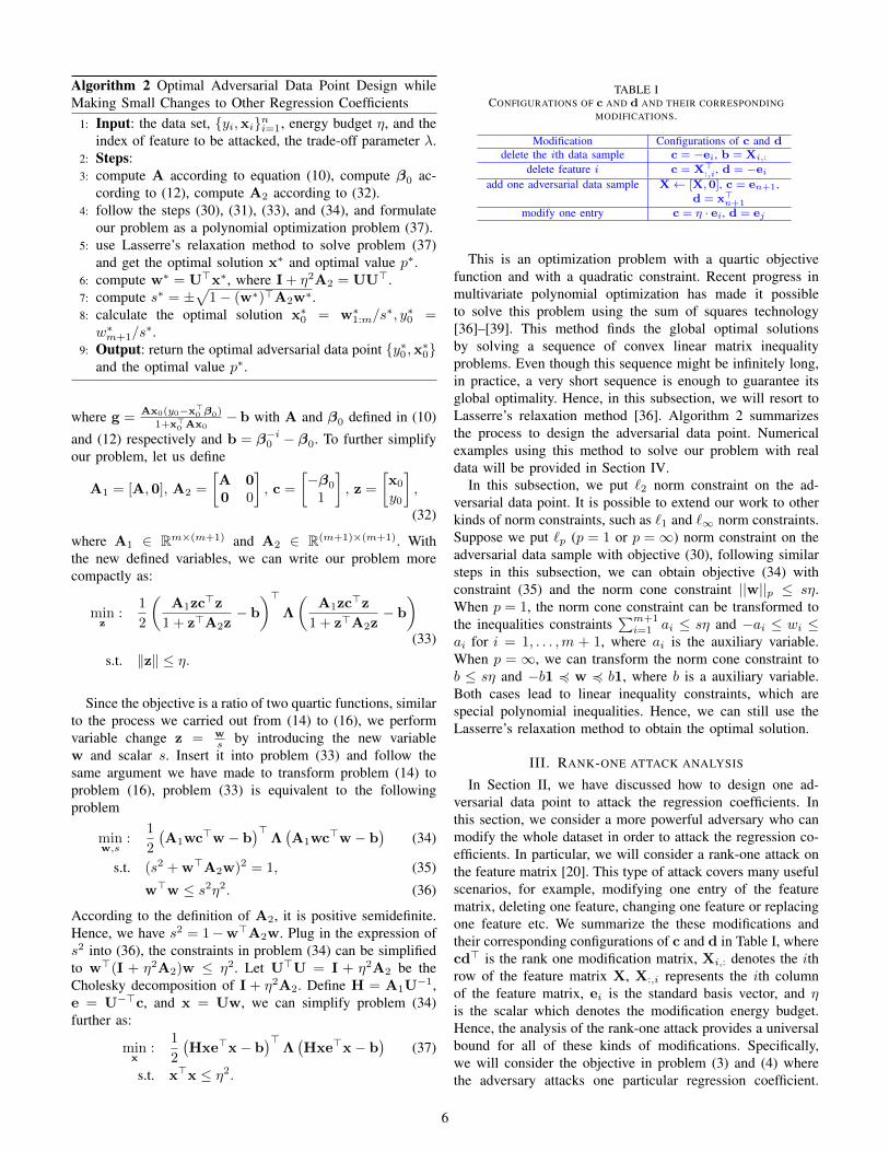
Algorithm 2 Optimal Adversarial Data Point Design whileMaking Small Changes to Other Regression Coefficients

1: Input: the data set, {yi,xi}ni=1, energy budget η, and theindex of feature to be attacked, the trade-off parameter λ.

2: Steps:3: compute A according to equation (10), compute β0 ac-

cording to (12), compute A2 according to (32).4: follow the steps (30), (31), (33), and (34), and formulate

our problem as a polynomial optimization problem (37).5: use Lasserre’s relaxation method to solve problem (37)

and get the optimal solution x∗ and optimal value p∗.6: compute w∗ = U>x∗, where I + η2A2 = UU>.7: compute s∗ = ±

√1− (w∗)>A2w∗.

8: calculate the optimal solution x∗0 = w∗1:m/s∗, y∗0 =

w∗m+1/s∗.

9: Output: return the optimal adversarial data point {y∗0 ,x∗0}and the optimal value p∗.

where g =Ax0(y0−x>

0 β0)

1+x>0 Ax0

−b with A and β0 defined in (10)

and (12) respectively and b = β−i0 − β0. To further simplifyour problem, let us define

A1 = [A,0], A2 =

[A 00 0

], c =

[−β0

1

], z =

[x0

y0

],

(32)

where A1 ∈ Rm×(m+1) and A2 ∈ R(m+1)×(m+1). Withthe new defined variables, we can write our problem morecompactly as:

minz

:1

2

(A1zc>z

1 + z>A2z− b

)>Λ

(A1zc>z

1 + z>A2z− b

)(33)

s.t. ‖z‖ ≤ η.

Since the objective is a ratio of two quartic functions, similarto the process we carried out from (14) to (16), we performvariable change z = w

s by introducing the new variablew and scalar s. Insert it into problem (33) and follow thesame argument we have made to transform problem (14) toproblem (16), problem (33) is equivalent to the followingproblem

minw,s

:1

2

(A1wc>w − b

)>Λ(A1wc>w − b

)(34)

s.t. (s2 + w>A2w)2 = 1, (35)

w>w ≤ s2η2. (36)

According to the definition of A2, it is positive semidefinite.Hence, we have s2 = 1−w>A2w. Plug in the expression ofs2 into (36), the constraints in problem (34) can be simplifiedto w>(I + η2A2)w ≤ η2. Let U>U = I + η2A2 be theCholesky decomposition of I + η2A2. Define H = A1U

−1,e = U−>c, and x = Uw, we can simplify problem (34)further as:

minx

:1

2

(Hxe>x− b

)>Λ(Hxe>x− b

)(37)

s.t. x>x ≤ η2.

TABLE ICONFIGURATIONS OF c AND d AND THEIR CORRESPONDING

MODIFICATIONS.

Modification Configurations of c and ddelete the ith data sample c = −ei, b = Xi,:

delete feature i c = X>:,i, d = −ei

add one adversarial data sample X← [X,0], c = en+1,d = x>

n+1

modify one entry c = η · ei, d = ej

This is an optimization problem with a quartic objectivefunction and with a quadratic constraint. Recent progress inmultivariate polynomial optimization has made it possibleto solve this problem using the sum of squares technology[36]–[39]. This method finds the global optimal solutionsby solving a sequence of convex linear matrix inequalityproblems. Even though this sequence might be infinitely long,in practice, a very short sequence is enough to guarantee itsglobal optimality. Hence, in this subsection, we will resort toLasserre’s relaxation method [36]. Algorithm 2 summarizesthe process to design the adversarial data point. Numericalexamples using this method to solve our problem with realdata will be provided in Section IV.

In this subsection, we put `2 norm constraint on the ad-versarial data point. It is possible to extend our work to otherkinds of norm constraints, such as `1 and `∞ norm constraints.Suppose we put `p (p = 1 or p =∞) norm constraint on theadversarial data sample with objective (30), following similarsteps in this subsection, we can obtain objective (34) withconstraint (35) and the norm cone constraint ||w||p ≤ sη.When p = 1, the norm cone constraint can be transformed tothe inequalities constraints

∑m+1i=1 ai ≤ sη and −ai ≤ wi ≤

ai for i = 1, . . . ,m + 1, where ai is the auxiliary variable.When p = ∞, we can transform the norm cone constraint tob ≤ sη and −b1 4 w 4 b1, where b is a auxiliary variable.Both cases lead to linear inequality constraints, which arespecial polynomial inequalities. Hence, we can still use theLasserre’s relaxation method to obtain the optimal solution.

III. RANK-ONE ATTACK ANALYSIS

In Section II, we have discussed how to design one ad-versarial data point to attack the regression coefficients. Inthis section, we consider a more powerful adversary who canmodify the whole dataset in order to attack the regression co-efficients. In particular, we will consider a rank-one attack onthe feature matrix [20]. This type of attack covers many usefulscenarios, for example, modifying one entry of the featurematrix, deleting one feature, changing one feature or replacingone feature etc. We summarize the these modifications andtheir corresponding configurations of c and d in Table I, wherecd> is the rank one modification matrix, Xi,: denotes the ithrow of the feature matrix X, X:,i represents the ith columnof the feature matrix, ei is the standard basis vector, and ηis the scalar which denotes the modification energy budget.Hence, the analysis of the rank-one attack provides a universalbound for all of these kinds of modifications. Specifically,we will consider the objective in problem (3) and (4) wherethe adversary attacks one particular regression coefficient.

6

In the following, we will first formulate our problem andthen provide our alternating optimization method to solve thisproblem.

In the considered rank one attack model, the attacker willcarefully design a rank-one feature modification matrix ∆ andadd it to the original feature matrix X. As the result, themodified feature matrix is X = X + ∆. As ∆ has rank one,we can write ∆ = cd>, where c ∈ Rn and d ∈ Rm. Similarto the previous section, we restrict the adversary to havingconstrained energy budget, η. Here, we use the Frobenius normto measure the energy of the modification matrix. Hence, wehave ‖∆‖F ≤ η, where ‖ · ‖F denotes the Frobenius norm ofa matrix. If the attacker’s goal is to increase the importanceof feature i, our problem can be written as

max‖cd>‖F≤η

: |βi| (38)

s.t. β = argminβ‖y − Xβ‖2,

X = X + cd>.

If the adversary is trying to minimize the magnitude of the ithregression coefficient, our problem is

min‖cd>‖F≤η

: |βi| (39)

s.t. β = argminβ

: ‖y − Xβ‖2,

X = X + cd>.

Similar to Section II-B, the solutions to problems (38) and (39)can be obtained by the solutions to the following two prob-lems:

max‖cd>‖F≤η

: βi (40)

and

min‖cd>‖F≤η

: βi (41)

with the same constraints as in (38) and (39).We can further write the above two problems in a more

unified form:

min‖cd>‖F≤η

: e>β (42)

s.t. β = argminβ

: ‖y − Xβ‖2,

X = X + cd>.

If e = ei, in which ei is a vector with the ith entry being1 and all other entries being zero, problem (42) is equivalentto problem (41). If e = −ei, problem (42) is equivalent toproblem (40). Hence, in the following part, we will focus onsolving this unified problem (42).

To solve problem (42), we can first solve the lower leveloptimization problem in the constraints. It admits a simplesolution that β = X†y and X† is the pseudo-inverse of X.

This pseudo-inverse can be written as X† = X† + G [40],where

G =1

γX†nw> − γ

‖n‖2‖w‖2 + γ2·(

‖w‖2

γX†n + v

)(‖n‖2

γw + n

)>, (43)

γ = 1 + d>X†c, v = X†c, n = (X†)>d, and w = (I −XX†)c.

Since β = X†y = (X†+ G)y and X† does not depend onc and d, our problem is equivalent to

minc,d

: e>Gy (44)

s.t. ‖c · d>‖F ≤ η.

Suppose (c∗,d∗) is the optimal solution of (44), it is easy tosee that for nonzero k, (kc∗,d∗/k) is also a valid optimalsolution. To avoid the ambiguity, it is necessary and possibleto further reduce the feasible region. Hence, we put an extraconstraint on c, where we restrict the norm of c to be lessthan or equal to 1. As the result, our problem can be furtherwritten as

minc,d

: e>Gy (45)

s.t. ‖c‖ ≤ 1, ‖d‖ ≤ η,

in which we use the identity ‖cd>‖F = ‖c‖‖d‖. It is clearthat problem (44) and problem (45) have the same optimalobjective value.

Since G is determined by c, d, and X, different values ofc and d may result in different objective functions. Beforefurther discussion, let us assume the singular value decompo-sition of the original feature matrix is X = UΣV>, whereΣ = [diag(σ1, σ2, · · · , σm),0]> and σ1 ≥ σ2 ≥ · · · ≥ σm >0. With this decomposition, we have X† = VΣ†U>, whereΣ† = [diag(σ−11 , σ−12 , · · · , σ−1m ),0]. In (43), if η ≥ σm, byletting γ → 0, we have our objective being minus infinity bysetting (c,d) = (um,−σmvm) or (c,d) = (−um, σmvm),where um and vm are the mth column of matrices U and V,respectively. Hence, we conclude that, when η ≥ σm, the op-timal value of problem (45) is unbounded from below. As theresult, throughout this section, we assume η < σm. Thus, wealso have γ = 1+d>X†c ≥ 1−‖c ·d>‖‖X†‖ ≥ 1− η

σm> 0.

We note that when η approaches σm, it does not mean to killall of the signals in the feature matrix but only some signalswith the energy equals to the smallest singular value of thefeature matrix.

Let h denote our objective h(c,d) = e>Gy, plug in theexpression of G, and we have

h(c,d) =1

‖n‖2‖w‖2 + γ2(γe>X†nw>y − γe>vn>y

− ‖w‖2e>X†nn>y − ‖n‖2e>vw>y). (46)

We need to optimize h(c,d) over c and d with the constraint‖c‖ ≤ 1 and ‖d‖ ≤ η. However, h(c,d) is a ratio of twoquartic functions, which is known to be a hard non-convexproblem in general. To solve this problem, similar to [32], wecan use the projected gradient descent method. However, it is

7

Algorithm 3 Optimal Rank-one Attack Matrix Design via theAlternating Optimization Algorithm

1: Input: data set {yi,xi}ni=1 and energy budget η.2: Initialize: randomly initialize c0 and d0, set number of

iterations k = 0.3: compute G according to (43).4: plug in the expression of G into (45), and obtain our

objective, h(c,d), as in (46).5: Do6: update ck by solving: ck = argmin

‖c‖≤1: h(c,dk−1),

7: update dk by solving: dk = argmin‖d‖≤η

: h(ck,d),

8: set k = k + 1,9: While convergence conditions are not meet.

10: compute the modification matrix ∆ = ck(dk)>.11: Output: return the modification matrix, ∆.

hard to choose a proper stepsize and its convergence is notclear when the projected gradient descent is used on a non-convex problem. In the following, we provide an alternatingoptimization algorithm with provable convergence.

The enabling observation of our approach is that, eventhough the optimization problem is a complex non-convexproblem, for a fixed c, h is a ratio of two quadratic functionswith respect to d. Similarly, for a fixed d, h is a ratio of twoquadratic functions with respect to c. A ratio of two quadraticfunctions admits a hidden convex structure [41]. Inspired bythis, we decompose our optimization variables into c and d,and then use alternating optimization algorithm described inAlgorithm 3 to sequentially optimize c and d.

The core of this algorithm is to solve the following twoproblems

ck = argmin‖c‖≤1

: h(c,dk−1), (47)

and

dk = argmin‖d‖≤η

: h(ck,d). (48)

For a fixed d, the objective of problem (47) becomes h(c,d) =h1(c)/h2(c), where we omit the superscript of d,

h1(c) = c>[e>X†nny>(I−XX†)− n>yne>X†

− e>X†nn>y(I−XX†)− ‖n‖2(X†)>ey>(I−XX†)]c

+[e>X†n(I−XX†)y − n>y(X†)>e

]>c, (49)

and

h2(c) =c>[‖n‖2(I−XX†) + nn>

]c + 2n>c + 1. (50)

Hence, problem (47) can be written as:

minc

:h1(c)

h2(c)(51)

s.t. ‖c‖ ≤ 1, (52)

where the forms of hi(c) = c>Aic + 2b>i c + li, i = 1, 2 andAi, bi and li can be derived from (49) and (50). The objectiveof this problem is the ration of two quadratic functions.

Even though it is non-convex, it has certain hidden convexstructures. The following theorem characterizes its optimalsolution by solving a semidefinite programming [41].

Theorem 1. ( [41]) If there exists µ > 0 such that[A2 b2

b>2 l2

]+ µ

[I 00 −1

]� 0, (53)

the optimal value of problem (51) is equivalent to thefollowing optimal value

maxα, ν≥0

: α (54)

s.t.[A1 b1

b>1 l1

]� α

[A2 b2

b>2 l2

]− ν

[I 00 −1

]Proof. Please see [41] for detail.

We now show that our problem (51) satisfies condition (53).As the result, we can find the solution to problem (51) bysolving problem (54).

To prove the left hand side of (53) is positive definite, wecan show the following two inequalities are true according toSchur complement condition for positive definite matrix

l2 − µ > 0, (55)

A2 + µI− 1

1− µb2b

>2 � 0, (56)

where l2 = 1. Plug in the expression of A2, the left hand ofinequality (56) can be written as

A2 + µI− 1

1− µb2b

>2

= ‖n‖2(I−XX†) + µI− µ

1− µnn>.

Since I − XX† is a projection matrix, it is positive semi-definite. So, we only need to prove

µI− µ

1− µnn> � 0. (57)

Since nn> is rank-one and its non-zero eigenvalue is ‖n‖2,it equals to proving ‖n‖2/(1 − µ) < 1. To guarantee thisinequality, we only need to make sure µ < 1 − ‖n‖2. Since‖X†‖ ≤ 1/σm and ‖d‖ ≤ η, we get ‖n‖2 = ‖(X†)>d‖2 ≤‖X†‖2‖d‖2 ≤ η2/σ2

m < 1. By choosing 0 < µ < 1−‖n‖2 <1, we can ensure (55) and (56) are both satisfied, and henceinequality (53) is satisfied.

From Theorem 1, we know the optimal value of (51) isequivalent to the optimal value of problem (54). Problem (54)is a semidefinite programming problem, which is convex andcan be easily solved by modern tools such as [42] and [43].We now discuss how to find the optimal c which achievesthis value. Suppose the optimal solution of problem (54) is(α∗, ν∗). Since, h2(c) > 0, we have h1(c) ≥ α∗h2(c) forany feasible c. Hence, we can compute the optimal solutionof problem (51) by solving

argminc

: h1(c)− α∗h2(c) (58)

s.t. ‖c‖2 ≤ 1 (59)

8

This problem is just a trust region problem. There are severalexisting methods to solve it efficiently. In this paper, weemploy the method described in [44].

Now, we turn to solve problem (48). Since (48) and (47)have similar structure, we can employ the methods describedin Theorem 1 and (58) to find its optimal value and optimalsolution for problem (48).

Until now, we have fully described how to solve theintermediate problems in the alternating optimization method.The following theorem shows that the proposed alternatingoptimization algorithm will converge. Suppose the generatedsequence of solution is {ck, dk}, k = 0, 1, · · · , and we havethe following corollary:

Corollary 1. The sequence {ck, dk} admits a limit point{c , d} and we have

limk→∞

h(ck,dk) = h(c, d). (60)

Furthermore, every limit point is a critical point, which means

∇h(c, d)>[

c− cd− d

]≥ 0, (61)

for any ‖c‖ ≤ 1 and ‖d‖ ≤ η.

Proof. We first give the proof of (60). Since the sequence{ck,dk} lies in the compact set, {(c,d) | ‖c‖ ≤ 1, ‖d‖ ≤η}, and according to the Bolzano-Weierstrass Theorem [45],{ck,dk} must have limit points. Hence, there is a subsequenceof {hk} which converges to h(c, d). As the objective is acontinuous function with respect to c and d, the compactnessof the constraint also implies the sequence of the objectivevalue, {hk}, is bounded from below. In addition, {hk} is anon-increasing sequence, which indicates that the sequence ofthe function value must converge. In summary, the sequence{hk} must converge to h(c, d). For the rest of the proof, pleaserefer to Corollary 2 of [46] for more details.

IV. NUMERICAL EXAMPLES

In this section, we test our adversarial attack strategies onpractical regression problems. In the first regression task, weuse seven international indexes to predict the returns of theIstanbul Stock Exchange [47]. The data set contains 536 datasamples, which are the records of the returns of Istanbul StockExchange with seven other international indexes starting fromJun. 5, 2009 to Feb. 22, 2011. Also, we demonstrate how ourattack impacts the quality of a regression task using the winedataset [48].

A. Attacking one specific regression coefficient

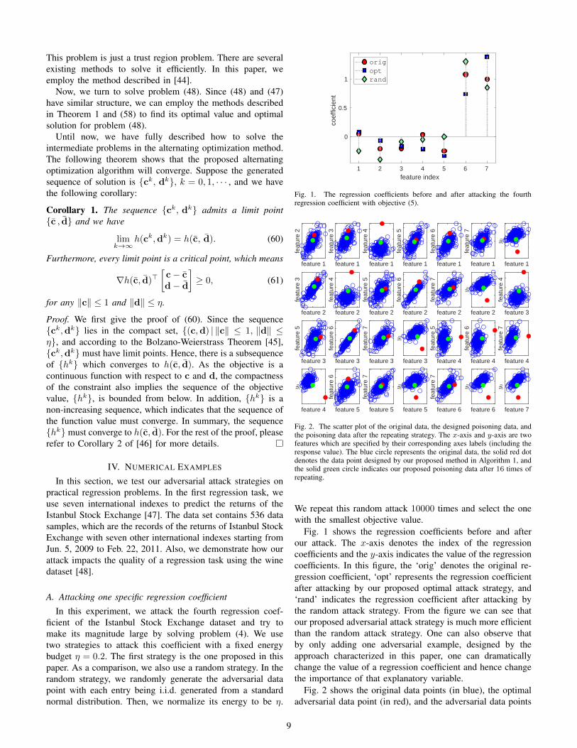
In this experiment, we attack the fourth regression coef-ficient of the Istanbul Stock Exchange dataset and try tomake its magnitude large by solving problem (4). We usetwo strategies to attack this coefficient with a fixed energybudget η = 0.2. The first strategy is the one proposed in thispaper. As a comparison, we also use a random strategy. In therandom strategy, we randomly generate the adversarial datapoint with each entry being i.i.d. generated from a standardnormal distribution. Then, we normalize its energy to be η.

0

0.5

1

co

eff

icie

nt

1 2 3 4 5 6 7

feature index

orig

opt

rand

Fig. 1. The regression coefficients before and after attacking the fourthregression coefficient with objective (5).

feature 1

fea

ture

2

feature 1

fea

ture

3

feature 1

fea

ture

4

feature 1

fea

ture

5

feature 1

fea

ture

6

feature 1

fea

ture

7

feature 1

feature 2

fea

ture

3

feature 2

fea

ture

4

feature 2

fea

ture

5

feature 2

fea

ture

6

feature 2

fea

ture

7

feature 2 feature 3

fea

ture

4

feature 3

fea

ture

5

feature 3

fea

ture

6

feature 3fe

atu

re 7

feature 3 feature 4

fea

ture

5

feature 4

fea

ture

6

feature 4

fea

ture

7

feature 4 feature 5

fea

ture

6

feature 5

fea

ture

7

feature 5 feature 6

fea

ture

7

feature 6 feature 7

Fig. 2. The scatter plot of the original data, the designed poisoning data, andthe poisoning data after the repeating strategy. The x-axis and y-axis are twofeatures which are specified by their corresponding axes labels (including theresponse value). The blue circle represents the original data, the solid red dotdenotes the data point designed by our proposed method in Algorithm 1, andthe solid green circle indicates our proposed poisoning data after 16 times ofrepeating.

We repeat this random attack 10000 times and select the onewith the smallest objective value.

Fig. 1 shows the regression coefficients before and afterour attack. The x-axis denotes the index of the regressioncoefficients and the y-axis indicates the value of the regressioncoefficients. In this figure, the ‘orig’ denotes the original re-gression coefficient, ‘opt’ represents the regression coefficientafter attacking by our proposed optimal attack strategy, and‘rand’ indicates the regression coefficient after attacking bythe random attack strategy. From the figure we can see thatour proposed adversarial attack strategy is much more efficientthan the random attack strategy. One can also observe thatby only adding one adversarial example, designed by theapproach characterized in this paper, one can dramaticallychange the value of a regression coefficient and hence changethe importance of that explanatory variable.

Fig. 2 shows the original data points (in blue), the optimaladversarial data point (in red), and the adversarial data points

9

0 0.5 1 1.5 2

-5

-4

-3

-2

-1

0

grad-avg

grad-min

rand

poly

(a)

0 0.5 1 1.5 2

0

0.1

0.2

0.3

0.4

0.5

0.6

0.7

grad-avg

grad-min

rand

poly

(b)

0 0.5 1 1.5 2

0

1

2

3

4

5

grad-avg

grad-min

rand

poly

(c)

Fig. 3. Attack the fourth regression coefficient with objective (30) and λ = −1 under different energy budgets.

-2

-1.5

-1

-0.5

0

0.5

1

1.5

coeffic

ient

1 2 3 4 5 6 7

feature index

orig

grad

rand

poly

Fig. 4. The regression coefficients before and after different kinds of strategiesthat attack the fourth regression coefficient with energy budget η = 1.

after the 16 times repeating strategy (in green) in this exper-iment. The figure demonstrates that the proposed adversarialdata point may behave as an outlier. However, after our simplerepeating strategy, the adversarial data points act just likenormal data points. Hence, our repeating strategy can mitigatethe adversarial data point being detected by the regressionsystem.

B. Attacking without changing untargeted regression coeffi-cients too much

From the numerical examples in the previous subsection, wecan see the untargeted regression coefficients may change dra-matically while we attacking one specific regression coefficientwith an adversarial data point. For example, as demonstratedin Fig. 1, the sixth and seventh regression coefficients changesignificantly when we attack the fourth regression coefficient.To mitigate the undesirable changes of untargeted regressioncoefficients, we need more sophisticated attacking strategies.In this subsection, we will test different strategies with a moregeneral objective function as demonstrated in Section II-C. Wealso use the same data set as described in the previous sub-section. We first try to attack the fourth regression coefficientto increase its importance while making only small changesto the rest of the regression coefficients. To accomplish thistask, we aim to solve problem (30) with λ = −1. Given theenergy budget, firstly, we use our semidefinite relaxation basedalgorithm to solve problem (37), and then follow Algorithm 2to find the adversarial data point. For comparison, we also

carry out the random attack strategy, in which we randomlygenerate the data point with each entry being i.i.d. accordingto the standard normal distribution. Then, we normalize itsenergy being η and added it to the original data points.We repeat these random attacks 10000 times and select theone with the smallest objective value. The third strategy isthe projected gradient descent based strategy, where we useprojected gradient descent algorithm to solve (37) and followsimilar steps of Algorithm 2 to find the adversarial datapoint. Projected gradient descent works much like the gradientdescent except with an additional operation that projects theresult of each step onto the feasible set after moving in thedirection of negative gradient [49]. In our experiment, we usediminishing stepsize, 1/(t + 1). Since the projected gradientdescent algorithm depends on the initial points heavily, giventhe energy budget, we repeat it 100 times with differentrandom initial points and treat the average of its objectivevalues as the objective value of this algorithm. Also, amongthe 100 times attacks, we record the one with the smallestobjective value.

Fig. 3 shows the objective values under different energybudgets with different attacking strategies and Fig. 4 demon-strates the regression coefficients after one of the attacks ofdifferent strategies with η = 1. In these figures, ‘orig’ isthe original regression coefficient, ‘rand’ means the randomstrategy, ‘poly’ indicates our semidefinite relaxation strategy,‘grad-avg’ is the average objective value of the 100 timesattacks based on projected gradient descent algorithm, and‘grad-min’ is the one with the smallest objective value amongthe 100 times attacks based on projected gradient descentalgorithm. From these two figures, we can see our semidefiniterelaxation based strategy performs much better than the othertwo strategies. Among the 100 times attacks based on pro-jected gradient descent, the minimal one can achieve similarobjective values as our proposed attacks based the semidefiniterelaxation. In addition, in our experiment, our semidefiniterelaxation method with relaxation order 2 or 3 can alwayslead to global optimal solutions. Hence, the computationalcomplexity of this method is still low. Fig. 4 also shows ourrelaxation based method leads to the largest magnitude of thefourth regression coefficient while keeping other regressioncoefficients almost unchanged.

In the second experiment, we attack the sixth regression

10

0 0.5 1 1.5 2

0

0.05

0.1

0.15

0.2

grad-avg

grad-min

rand

poly

(a)

0 0.5 1 1.5 2

0

0.05

0.1

0.15

grad-avg

grad-min

rand

poly

(b)

0 0.5 1 1.5 2

0

0.02

0.04

0.06

0.08

0.1

grad-avg

grad-min

rand

poly

(c)

Fig. 5. Attack the sixth regression coefficient with objective (30) and λ = 1 under different energy budgets.

-0.4

-0.2

0

0.2

0.4

0.6

0.8

1

1.2

coeffic

ient

1 2 3 4 5 6 7

feature index

orig

grad

rand

poly

Fig. 6. The regression coefficients after different kinds of strategies that attackthe sixth regression coefficient with energy budget η = 1.

0.2 0.4 0.6 0.8 1

/m

-2

-1.5

-1

-0.5

0

obje

ctive v

alu

e

GD-1

GD-10

GD-100

AO

Fig. 7. The averaged objective values of the projected gradient descent withdifferent stepsizes and the proposed alternating optimization method.

coefficient and attempt to make its magnitude small whilekeeping the change of the rest of the coefficients to besmall. So, we set λ = 1 in problem (30) to achieve thisgoal. The settings of each strategy is similar to the ones inthe first experiment. Fig. 5 shows the objective values withdifferent strategies under different energy budgets and Fig. 6demonstrates the regression coefficients after one of the attacksof those strategies respectively with energy budget η = 1.From Fig. 5 we know the projected gradient descent basedstrategy and semidefinite relaxation based strategy achievemuch lower objective values compared to the random attackstrategy. Specifically, when the energy budget is smaller than0.7, both of the two strategies behave similarly. However, whenthe energy budget is larger than 0.7, the projected gradient

descent based strategy leads to larger objective values as theenergy budget grows. This is because the projected gradientdescent algorithm tends to find solutions at the boundary ofthe feasible set. Only some attacks with good initializationcan lead to the global minimum. By contrast, our semidefiniterelaxation based strategy can find the global optimal solutionswith relaxation order 2 or 3. Thus, it gives the best perfor-mance among the three strategies. Fig. 6 also demonstrates ourrelaxation based method achieves the global optimum whenη = 1 as it leads the sixth regression coefficient to zero andother regression coefficients to be unchanged.

C. Rank-one attack

In this subsection, we carry out different rank-one attackstrategies. Our goal is to minimize the magnitude of the fourthregression coefficient with objective (41). We compare twostrategies: the projected gradient descent based strategy dis-cussed in Section IV-B and our proposed alternating optimiza-tion based strategy. For the projected gradient descent basedstrategies, we use different step sizes: 1/(1+t), 10/(1+t), and100/(1 + t). As our analysis shows, when the energy budgetis larger than the smallest singular value, our objective can beminus infinity. Hence, in our experiment, we vary the energybudget from 0 to the smallest singular value, which is 0.053.Given a certain energy budget, we set all the algorithms withthe same randomly initialized point and run these algorithmsuntil they stop with the same convergence condition that is twoconsecutive function values change too small or it reaches themaximal allowable iterations. We repeat this process 100 timesand record their average objective values.

Fig. 7 shows the averaged objective values of the four al-gorithms, where ‘GD-1’, ‘GD-10’ and ‘GD-100’ stand for theprojected gradient descent with stepsizes 1/(1+t), 10/(1+t),and 100/(1 + t), respectively, and ‘AO’ denotes the proposedalternating optimization method. As Fig. 7 shows, when theenergy budget increases, the objectives decrease for bothof these algorithms. Furthermore, the proposed alternatingoptimization based algorithm provides much smaller objectivevalues, especially when the energy budget approaches thesmallest singular value. When the energy budget approachesthe smallest singular value, the gradient descent based algo-rithm becomes very unstable. This is due to the fact that whenthe energy budget is large, the objective is very sensitive to theenergy budget. So, a small stepsize may result in significant

11

0 50 100 150 200

iteration

-20

-15

-10

-5

0

obje

ctive v

alu

e

10-3

GD

AO

(a)

0 20 40 60 80

iteration

-0.1

-0.08

-0.06

-0.04

-0.02

0

0.02

ob

jective

va

lue

GD

AO

(b)

0 50 100 150 200 250 300

iteration

-0.15

-0.1

-0.05

0

0.05

0.1

obje

ctive v

alu

e

GD

AO

(c)

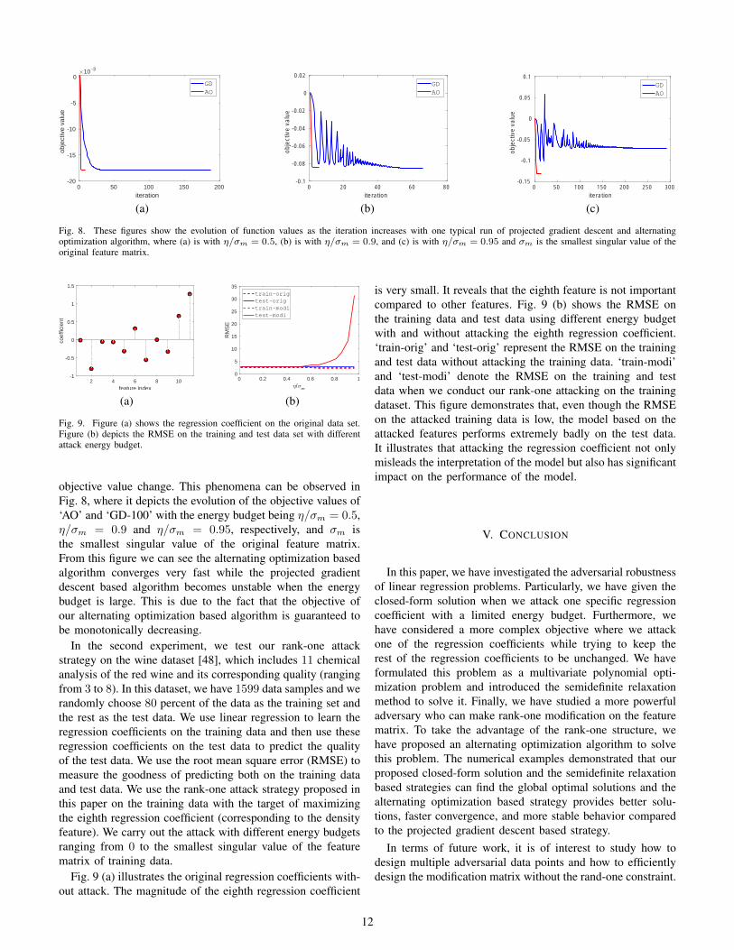
Fig. 8. These figures show the evolution of function values as the iteration increases with one typical run of projected gradient descent and alternatingoptimization algorithm, where (a) is with η/σm = 0.5, (b) is with η/σm = 0.9, and (c) is with η/σm = 0.95 and σm is the smallest singular value of theoriginal feature matrix.

-1

-0.5

0

0.5

1

1.5

co

eff

icie

nt

2 4 6 8 10

feature index

(a)

0 0.2 0.4 0.6 0.8 1

/m

0

5

10

15

20

25

30

35

RM

SE

train-orig

test-orig

train-modi

test-modi

(b)

Fig. 9. Figure (a) shows the regression coefficient on the original data set.Figure (b) depicts the RMSE on the training and test data set with differentattack energy budget.

objective value change. This phenomena can be observed inFig. 8, where it depicts the evolution of the objective values of‘AO’ and ‘GD-100’ with the energy budget being η/σm = 0.5,η/σm = 0.9 and η/σm = 0.95, respectively, and σm isthe smallest singular value of the original feature matrix.From this figure we can see the alternating optimization basedalgorithm converges very fast while the projected gradientdescent based algorithm becomes unstable when the energybudget is large. This is due to the fact that the objective ofour alternating optimization based algorithm is guaranteed tobe monotonically decreasing.

In the second experiment, we test our rank-one attackstrategy on the wine dataset [48], which includes 11 chemicalanalysis of the red wine and its corresponding quality (rangingfrom 3 to 8). In this dataset, we have 1599 data samples and werandomly choose 80 percent of the data as the training set andthe rest as the test data. We use linear regression to learn theregression coefficients on the training data and then use theseregression coefficients on the test data to predict the qualityof the test data. We use the root mean square error (RMSE) tomeasure the goodness of predicting both on the training dataand test data. We use the rank-one attack strategy proposed inthis paper on the training data with the target of maximizingthe eighth regression coefficient (corresponding to the densityfeature). We carry out the attack with different energy budgetsranging from 0 to the smallest singular value of the featurematrix of training data.

Fig. 9 (a) illustrates the original regression coefficients with-out attack. The magnitude of the eighth regression coefficient

is very small. It reveals that the eighth feature is not importantcompared to other features. Fig. 9 (b) shows the RMSE onthe training data and test data using different energy budgetwith and without attacking the eighth regression coefficient.‘train-orig’ and ‘test-orig’ represent the RMSE on the trainingand test data without attacking the training data. ‘train-modi’and ‘test-modi’ denote the RMSE on the training and testdata when we conduct our rank-one attacking on the trainingdataset. This figure demonstrates that, even though the RMSEon the attacked training data is low, the model based on theattacked features performs extremely badly on the test data.It illustrates that attacking the regression coefficient not onlymisleads the interpretation of the model but also has significantimpact on the performance of the model.

V. CONCLUSION

In this paper, we have investigated the adversarial robustnessof linear regression problems. Particularly, we have given theclosed-form solution when we attack one specific regressioncoefficient with a limited energy budget. Furthermore, wehave considered a more complex objective where we attackone of the regression coefficients while trying to keep therest of the regression coefficients to be unchanged. We haveformulated this problem as a multivariate polynomial opti-mization problem and introduced the semidefinite relaxationmethod to solve it. Finally, we have studied a more powerfuladversary who can make rank-one modification on the featurematrix. To take the advantage of the rank-one structure, wehave proposed an alternating optimization algorithm to solvethis problem. The numerical examples demonstrated that ourproposed closed-form solution and the semidefinite relaxationbased strategies can find the global optimal solutions and thealternating optimization based strategy provides better solu-tions, faster convergence, and more stable behavior comparedto the projected gradient descent based strategy.

In terms of future work, it is of interest to study how todesign multiple adversarial data points and how to efficientlydesign the modification matrix without the rand-one constraint.

12

REFERENCES

[1] X. Yan and X. Su, Linear regression analysis: theory and computing.World Scientific, 2009.

[2] G. Papageorgiou, P. Bouboulis, and S. Theodoridis, “Robust linearregression analysis— a greedy approach,” IEEE Transactions on SignalProcessing, vol. 63, no. 15, pp. 3872–3887, Aug. 2015.

[3] X. Jiang, W. Zeng, H. C. So, A. M. Zoubir, and T. Kirubarajan,“Beamforming via nonconvex linear regression,” IEEE Transactions onSignal Processing, vol. 64, no. 7, pp. 1714–1728, Apr. 2016.

[4] J. Chien and J. Chen, “Recursive Bayesian linear regression for adaptiveclassification,” IEEE Transactions on Signal Processing, vol. 57, no. 2,pp. 565–575, Feb. 2009.

[5] T. Gustafsson and B. D. Rao, “Statistical analysis of subspace-basedestimation of reduced-rank linear regressions,” IEEE Transactions onSignal Processing, vol. 50, no. 1, pp. 151–159, Jan. 2002.

[6] R. Tibshirani, “Regression shrinkage and selection via the lasso,” Jour-nal of the Royal Statistical Society: Series B (Methodological), vol. 58,no. 1, pp. 267–288, 1996.

[7] J. H. McDonald, Handbook of biological statistics. Sparky HousePublishing, 2009.

[8] O. E. Barndorff-Nielsen and N. Shephard, “Econometric analysis ofrealized covariation: High frequency based covariance, regression, andcorrelation in financial economics,” Econometrica, vol. 72, no. 3, pp.885–925, May 2004.

[9] C. J. ter Braak and S. Juggins, “Weighted averaging partial least squaresregression (WA-PLS): an improved method for reconstructing envi-ronmental variables from species assemblages,” in Proc. InternationalDiatom Symposium, Renesse, The Netherlands, Aug. 1993, pp. 485–502.

[10] S. G. Finlayson, J. D. Bowers, J. Ito, J. L. Zittrain, A. L. Beam, and I. S.Kohane, “Adversarial attacks on medical machine learning,” Science,vol. 363, no. 6433, pp. 1287–1289, Mar. 2019.

[11] A. E. Sallab, M. Abdou, E. Perot, and S. Yogamani, “Deep reinforcementlearning framework for autonomous driving,” Electronic Imaging, vol.2017, no. 19, pp. 70–76, Jan. 2017.

[12] I. Goodfellow, J. Shlens, and C. Szegedy, “Explaining and harnessingadversarial examples,” arXiv:1412.6572, Dec. 2014.

[13] A. Kurakin, I. Goodfellow, and S. Bengio, “Adversarial machine learningat scale,” arXiv:1611.01236, Nov. 2016.

[14] I. Goodfellow, P. McDaniel, and N. Papernot, “Making machine learningrobust against adversarial inputs,” Communications of the ACM, vol. 61,no. 7, pp. 56–66, Jun. 2018.

[15] L. G. Hafemann, R. Sabourin, and L. S. Oliveira, “Characterizingand evaluating adversarial examples for offline handwritten signatureverification,” IEEE Transactions on Information Forensics and Security,vol. 14, no. 8, pp. 2153–2166, Aug. 2019.

[16] W. Tang, B. Li, S. Tan, M. Barni, and J. Huang, “CNN-based adversarialembedding for image steganography,” IEEE Transactions on InformationForensics and Security, vol. 14, no. 8, pp. 2074–2087, Aug. 2019.

[17] D. Li and Q. Li, “Adversarial deep ensemble: Evasion attacks anddefenses for malware detection,” IEEE Transactions on InformationForensics and Security, vol. 15, pp. 3886–3900, Jun. 2020.

[18] X. Chen, C. Liu, B. Li, K. Lu, and D. Song, “Targeted backdoor attackson deep learning systems using data poisoning,” arXiv:1712.05526, Dec.2017.

[19] S. Boyd and L. Vandenberghe, Convex optimization. CambridgeUniversity Press, 2004.

[20] F. Li, L. Lai, and S. Cui, “On the adversarial robustness of subspacelearning,” IEEE Transactions on Signal Processing, vol. 68, pp. 1470–1483, Mar. 2020.

[21] D. L. Pimentel-Alarcon, A. Biswas, and C. R. Solıs-Lemus, “Adversarialprincipal component analysis,” in Proc. IEEE International Symposiumon Information Theory, Aachen, Germany, Jun. 2017, pp. 2363–2367.

[22] S. Alfeld, X. Zhu, and P. Barford, “Data poisoning attacks against autore-gressive models,” in Proc. AAAI Conference on Artificial Intelligence,Phoenix, Arizona, Feb. 2016, pp. 1452–1458.

[23] M. Jagielski, A. Oprea, B. Biggio, C. Liu, C. Nita-Rotaru, and B. Li,“Manipulating machine learning: Poisoning attacks and countermeasuresfor regression learning,” in Proc. IEEE Symposium on Security andPrivacy, San Francisco, CA, May 2018, pp. 19–35.

[24] B. Biggio, B. Nelson, and P. Laskov, “Poisoning attacks against sup-port vector machines,” in Proc. International Conference on MachineLearning, Edinburgh, Scotland, Jun. 2012, pp. 1807–1814.

[25] ——, “Support vector machines under adversarial label noise,” in Proc.Asian Conference on Machine Learning, Taoyuan, Taiwan, Nov. 2011,pp. 97–112.

[26] X. Yuan, P. He, Q. Zhu, and X. Li, “Adversarial examples: Attacks anddefenses for deep learning,” IEEE transactions on neural networks andlearning systems, vol. 30, no. 9, pp. 2805–2824, Sep. 2019.

[27] T. Gu, K. Liu, B. Dolan-Gavitt, and S. Garg, “Badnets: Evaluatingbackdooring attacks on deep neural networks,” IEEE Access, vol. 7,pp. 47 230–47 244, Apr. 2019.

[28] Y. Chen, H. Xu, C. Caramanis, and S. Sanghavi, “Robust matrixcompletion and corrupted columns,” in Proc. International Conferenceon Machine Learning, Bellevue, Washington, Jun. 2011, pp. 873–880.

[29] B. Biggio and F. Roli, “Wild patterns: Ten years after the rise ofadversarial machine learning,” Pattern Recognition, vol. 84, pp. 317–331, Dec. 2018.

[30] H. Kwon, Y. Kim, H. Yoon, and D. Choi, “Selective audio adversarialexample in evasion attack on speech recognition system,” IEEE Trans-actions on Information Forensics and Security, vol. 15, pp. 526–538,Jun. 2019.

[31] B. Flowers, R. M. Buehrer, and W. C. Headley, “Evaluating adversarialevasion attacks in the context of wireless communications,” IEEETransactions on Information Forensics and Security, vol. 15, pp. 1102–1113, Aug. 2019.

[32] S. Mei and X. Zhu, “Using machine teaching to identify optimaltraining-set attacks on machine learners,” in Proc. AAAI Conference onArtificial Intelligence, Austin, Texas, Jan. 2015, pp. 2871–2877.

[33] R. A. Horn and C. R. Johnson, Matrix analysis. Cambridge UniversityPress, 2012.

[34] A. Beck and M. Teboulle, “On minimizing quadratically constrainedratio of two quadratic functions,” Journal of Convex Analysis, vol. 17,no. 3, pp. 789–804, 2010.

[35] A. Konar and N. D. Sidiropoulos, “Fast approximation algorithms for aclass of non-convex QCQP problems using first-order methods,” IEEETransactions on Signal Processing, vol. 65, no. 13, pp. 3494–3509, Apr.2017.

[36] J. B. Lasserre, “Global optimization with polynomials and the problemof moments,” SIAM Journal on Optimization, vol. 11, no. 3, pp. 796–817, 2001.

[37] M. Laurent, “Sums of squares, moment matrices and optimizationover polynomials,” in Emerging Applications of Algebraic Geometry.Springer, 2009, pp. 157–270.

[38] T. Weisser, J. B. Lasserre, and K.-C. Toh, “Sparse-BSOS: a boundeddegree SOS hierarchy for large scale polynomial optimization withsparsity,” Mathematical Programming Computation, vol. 10, no. 1, pp.1–32, 2018.

[39] M. J. Wainwright and M. I. Jordan, “Log-determinant relaxation forapproximate inference in discrete markov random fields,” IEEE trans-actions on signal processing, vol. 54, no. 6, pp. 2099–2109, Jun. 2006.

[40] K. B. Petersen and M. S. Pedersen, “The matrix cookbook,” TechnicalUniversity of Denmark, 2008.

[41] A. Beck and M. Teboulle, “A convex optimization approach for min-imizing the ratio of indefinite quadratic functions over an ellipsoid,”Mathematical Programming, vol. 118, no. 1, pp. 13–35, Apr. 2009.

[42] F. Rendl, “A matlab toolbox for semidefinite programming,”The program can be found at ftp://orion. uwaterloo.ca/pub/henry/teaching/co769g, 1994.

[43] J. Lofberg, “Yalmip: A toolbox for modeling and optimization inmatlab,” in Proc. International Conference on Robotics and Automation,New Orleans, LA, Apr. 2004, pp. 284–289.

[44] A. Beck, A. Ben-Tal, and M. Teboulle, “Finding a global optimalsolution for a quadratically constrained fractional quadratic problem withapplications to the regularized total least squares,” SIAM Journal onMatrix Analysis and Applications, vol. 28, no. 2, pp. 425–445, 2006.

[45] R. G. Bartle and D. R. Sherbert, Introduction to real analysis. WileyNew York, 2000.

[46] L. Grippo and M. Sciandrone, “On the convergence of the blocknonlinear Gauss–Seidel method under convex constraints,” OperationsResearch Letters, vol. 26, no. 3, pp. 127–136, Apr. 2000.

[47] O. Akbilgic, H. Bozdogan, and M. E. Balaban, “A novel hybrid RBFneural networks model as a forecaster,” Statistics and Computing,vol. 24, no. 3, pp. 365–375, May 2014.

[48] D. Dua and C. Graff, “UCI machine learning repository,” 2017.[Online]. Available: http://archive.ics.uci.edu/ml

[49] N. Parikh and S. Boyd, “Proximal algorithms,” Foundations andTrends R© in Optimization, vol. 1, no. 3, pp. 127–239, Jan. 2014.

13