Optimal Multiple Stopping Approach to Mean Reversion Trading Xin Li Submitted in partial fulfillment of the requirements for the degree of Doctor of Philosophy in the Graduate School of Arts and Sciences COLUMBIA UNIVERSITY 2015
Transcript
Optimal Multiple Stopping Approachto Mean Reversion Trading
2.1 MLE estimates of OU process parameters . . . . . . . . . . . 13
v
Acknowledgments
The compilation and completion of this dissertation marks the end of my
journey as a doctoral student and signals the commencement of the next stage
of my life. I am extremely fortunate to be able to spend five years at the
Department of Industrial Engineering and Operations at Columbia University
working alongside exceptional academic researchers and forging friendships
with some of the most brilliant people that I have the privilege of meeting.
The knowledge and experience that I have acquired as a PhD student is a
valuable source of wisdom that will benefit me in future endeavors.
First and foremost, my achievements would not be possible without the
continued support of my advisor, Professor Tim Leung. Professor Leung has
devoted much time and effort in seeking a research topic that not only makes
use of my strengths but also challenges me. Throughout our collaboration,
Professor Leung has been very supportive and often comes up with interesting
ideas that inspires me. Professor Leung’s constant motivation and encourage-
ment has helped me overcome many obstacles. As a role model, Professor
Leung is very intelligent and enthusiastic; he takes great pride in his work and
has remarkable insights in the field of quantitative finance. In the face of chal-
lenges, Professor Leung never fails to display confidence and optimism. This
attribute influences the people around him and is in particular, an inspiration
to his students. Under his tutelage, I have matured both as an academic pro-
fessional and as a person. I am immensely grateful for his help and guidance.
I am also grateful to members of my dissertation committee: Professor
vi
David Yao, Professor Mariana Olvera-Cravioto, Professor Hongzhong Zhang
and Professor Victor de la Pena for their careful reading of my thesis manuscript
and providing constructive comments.
I also wish to express my sincere gratitude to Professor David Yao, Pro-
fessor Ward Whitt and Professor Donald Goldfarb for believing in me and
encouraging me to apply for the doctoral program. I am thankful for the op-
portunity to become a member of the IEOR family. This was only made pos-
sible by their support. In addition, taking their doctoral courses in stochastic
processes and optimization as a masters student introduced me to the fascinat-
ing world of operations research and equipped me with the tools and resources
to conduct academic research. They are not only foremost researchers in their
fields but also excellent teachers. In addiiton, I wish to thank Professor Daniel
Bienstock, Professor Emmanuel Derman, Professor Martin Haugh, Professor
Xuedong He, Professor Jay Sethuraman and Professor Cliff Stein. The courses
I took with them broadened my perspective.
I would like to thank all my fellow PhD students of the department for
their sincere friendship and for all the good and bad time we have shared
together. I wish to express my sincere gratitude to Ningyuan Chen, Brian Lu,
Bo Huang, Marco Santoli, Aya Wallwater, Carlos Adrian Abad Lopez, Xinyun
Chen, Juan Li, Chun Wang, Jing Dong, Yupeng Chen, Chen Chen, Zhen Qiu,
Jinbeom Kim, Hailey Song Hee Kim, Yunan Liu, Shiqian Ma, Haowen Zhong,
Zhiwei Qin, Xingbo Xu, Yina Lu, Jing Guo, Cun Mu, Chun Ye, Linan Yang,
Anran Li, Antoine Desir, Itai Feigenbaum, Di Xiao, Liao Wang, Ni Ma, Yanan
Pei, Fei He.
I am deeply indebted to my parents for their unconditional love and support
throughout the years. No words can express my gratitude to them. Last but
not the least, I give my most special thanks to my husband, Zheng Wang, for
being with me along this journey.
vii
To my parents and my husband
viii
CHAPTER 1. INTRODUCTION 1
Chapter 1
Introduction
One important problem commonly faced by individual and institutional in-
vestors is to determine when to open and close a position. While observing
the prevailing market prices, a speculative investor can choose to enter the
market immediately or wait for a future opportunity. After completing the
first trade, the investor will need to decide when is the best to close the po-
sition. This motivates the investigation of the optimal sequential timing of
trades.
Naturally, the optimal sequence of trading times should depend on the price
dynamics of the risky asset. For instance, if the price process is a super/sub-
martingale, then the investor, who seeks to maximize the expected liquidation
value, will either sell immediately or wait forever. Such a trivial timing arises
when the underlying price follows a geometric Brownian motion (see Example
A below). Similar observations can also be found in, among others, Shiryaev
et al. [2008].
On the other hand, it has been widely observed that many asset prices ex-
hibit mean reversion, including commodities (see Schwartz [1997]), foreign ex-
change rates (see Engel and Hamilton [1989]; Anthony and MacDonald [1998];
Larsen and Sørensen [2007]), volatility indices (see Metcalf and Hassett [1995],
CHAPTER 1. INTRODUCTION 2
Bessembinder et al. [1995], Casassus and Collin-Dufresne [2005], and references
therein), as well as US and global equities (see Poterba and Summers [1988];
Malliaropulos and Priestley [1999]; Balvers et al. [2000]; Gropp [2004]). Mean-
reverting processes are also used to model the dynamics of interest rate, and
default risk. In industry, hedge fund managers and investors often attempt
to construct mean-reverting prices by simultaneously taking positions in two
highly correlated or co-moving assets. The advent of exchange-traded funds
(ETFs) has further facilitated this pairs trading approach since some ETFs
are designed to track identical or similar indexes and assets. For instance,
Triantafyllopoulos and Montana [2011] investigate the mean-reverting spreads
between commodity ETFs and design model for statistical arbitrage. Dunis
et al. [2013] also examine the mean-reverting spread between physical gold and
gold equity ETFs.
In this thesis, we study the optimal timing of trades under the Ornstein-
Uhlenbeck (OU), exponential Ornstein-Uhlenbeck (XOU), or Cox-Ingersoll-
Ross (CIR) model. In Chapter 2, we discuss a pairs trading example where
we model the value of resulting position by an OU process. To incorporate
mean-reversion for positive price processes, one popular choice for pricing and
investment applications is the exponential OU model, as proposed by Schwartz
[1997] for commodity prices, due to its analytical tractability. It also serves
as the building block of more sophisticated mean-reverting models. The CIR
process has been widely used as the model for short interest rates, volatility,
and energy prices (see, for example, Cox et al. [1985], Heston [1993], Ribeiro
and Hodges [2004], respectively). In the real option literature, mean reverting
processes have been used to model the value of a project. For instance, Ewald
and Wang [2010] studies the timing of an irreversible investment whose value
is modeled by a CIR process, and they solve the associated optimal single
stopping problem. Carmona and Leon [2007] examine the optimal investment
CHAPTER 1. INTRODUCTION 3
timing where the interest rate evolves according to a CIR process.
In Chapter 2, we study the optimal timing of trades subject to transaction
costs under the OU model. Specifically, our formulation leads to an optimal
double stopping problem that gives the optimal entry and exit decision rules.
We obtain analytic solutions for both the entry and exit problems. In addition,
we incorporate a stop-loss constraint to our trading problem. We find that a
higher stop-loss level induces the investor to voluntarily liquidate earlier at
a lower take-profit level. Moreover, the entry region is characterized by a
bounded price interval that lies strictly above stop-loss level. In other words,
it is optimal to wait if the current price is too high or too close to the lower stop-
loss level. This is intuitive since entering the market close to stop-loss implies
a high chance of exiting at a loss afterwards. As a result, the delay region
(complement of the entry region) is disconnected. Furthermore, we show that
optimal liquidation level decreases with the stop-loss level until they coincide,
in which case immediate liquidation is optimal at all price levels. Chapter 2
is adapted from Leung and Li [2015].
In Chapter 3, we study the optimal timing of trades under the XOU model.
We consider the optimal double stopping problem, as well as a different but re-
lated formulation. In the second formulation, the investor is assumed to enter
and exit the market infinitely many times with transaction costs. This gives
rise to an optimal switching problem. We analytically derive the non-trivial
entry and exit timing strategies. Under both approaches, it is optimal to sell
when the asset price is sufficiently high, though at different levels. As for entry
timing, we find that, under some conditions, it is optimal for the investor not
to enter the market at all when facing the optimal switching problem. In this
case for the investor who has a long position, the optimal switching problem
reduces into an optimal stopping problem, where the optimal liquidation level
is identical to that of the optimal double stopping problem. Otherwise, the
CHAPTER 1. INTRODUCTION 4
optimal entry timing strategies for the double stopping and switching problem
are described by the underlying’s first passage time to an interval that lies
above level zero. In other words, the continuation region for entry is discon-
nected of the form (0, A) ∪ (B,+∞), with critical price levels A and B (see
Theorems 3.2.4 and 3.2.7 below). This means that the investor generally en-
ters when the price is low, but may find it optimal to wait if the current price
is too close to zero. We find that this phenomenon is a distinct consequence
due to fixed transaction costs under the XOU model. Indeed, when there is
no fixed costs, even if there are proportional transaction costs (see Zhang and
Zhang [2008]), the entry timing is simply characterized by a single price level.
Chapter 3 is based on Leung et al. [2014a].
Our main contribution in Chapter 4 is the analytical derivation of the
non-trivial optimal entry and exit timing strategies and the associated value
functions. Under both double stopping and switching approaches, it is optimal
to exit when the process value is sufficiently high, though at different levels.
As for entry timing, we find the necessary and sufficient conditions whereby it
is optimal not to enter at all when facing the optimal switching problem. In
this case, the optimal switching problem in fact reduces to an optimal single
stopping problem, where the optimal stopping level is identical to that of the
optimal double stopping problem. Chapter 4 is built on Leung et al. [2014b].
A typical solution approach for optimal stopping problems driven by diffu-
sion involves the analytical and numerical studies of the associated free bound-
ary problems or variational inequalities (VIs); see e.g. Bensoussan and Lions
[1982], Øksendal [2003], and Sun [1992]. For our double optimal stopping
problem, this method would determine the value functions from a pair of VIs
and require regularity conditions to guarantee that the solutions to the VIs
indeed correspond to the optimal stopping problems. As noted by Dayanik
[2008], “the variational methods become challenging when the form of the re-
CHAPTER 1. INTRODUCTION 5
ward function and/or the dynamics of the diffusion obscure the shape of the
optimal continuation region.” In our optimal entry timing problem, the reward
function involves the value function from the exit timing problem, which is not
monotone and can be positive and negative.
In contrast to the variational inequality approach, our proposed methodol-
ogy starts with a characterization of the value functions as the smallest concave
majorant of any given reward function. A key feature of this approach is that
it allows us to directly construct the value function, without a priori finding
a candidate value function or imposing conditions on the stopping and delay
(continuation) regions, such as whether they are connected or not. In other
words, our method will derive the structure of the stopping and delay regions
as an output.
Having solved the optimal double stopping problem, we determine the
optimal structures of the buy/sell/wait regions. We then apply this to infer a
similar solution structure for the optimal switching problem and verify using
the variational inequalities.
In earlier studies, Dynkin and Yushkevich [1969] analyze the concave char-
acterization of excessive functions for a standard Brownian motion, and Dayanik
and Karatzas [2003] and Dayanik [2008] apply this idea to study the optimal
single stopping of a one-dimensional diffusion. Alvarez [2003] discusses the
conditions for the convexity of an r-excessive mapping under a linear, time-
homogeneous and regular diffusion process. In this regard, we contribute to
this line of work by solving a number of optimal double stopping problems
under the OU, XOU, or CIR model, and incorporating a stop-loss exit under
the OU model.
Among other related studies, Ekstrom et al. [2011] analyze the optimal
single liquidation timing under the OU model with zero long-run mean and
no transaction cost. Chapter 2 extends their model in a number of ways.
CHAPTER 1. INTRODUCTION 6
First, we analyze the optimal entry timing as well as the optimal liquidation
timing. Our model allows for a non-zero long-run mean and transaction costs,
along with a stop-loss level. Song et al. [2009] propose a numerical stochastic
approximation scheme to solve for the optimal buy-low-sell-high strategies over
a finite horizon. Song and Zhang [2013] study the optimal switching problem
with stop-loss under the OU price dynamics. Under a similar setting, Zhang
and Zhang [2008] and Kong and Zhang [2010] also investigate the infinite
sequential buying and selling/shorting problem under exponential OU price
dynamics with slippage cost. In contrast to these studies, we study both
optimal double stopping and switching problems specifically under exponential
OU with fixed transaction costs. In particular, the optimal entry timing with
fixed transaction costs is characteristically different from that with slippage.
Zervos et al. [2013] consider an optimal switching problem with fixed trans-
action costs under a class of time-homogeneous diffusions, including the GBM,
mean-reverting CEV underlying, and other models. However, their results are
not applicable to the exponential OU model as it violates Assumption 4 of
their paper (see also Remark 3.3.4 below). Indeed, their model assumptions
restrict the optimal entry region to be represented by a single critical thresh-
old, whereas we show that in the XOU model the optimal entry region is
characterized by two positive price levels.
As for related applications of optimal stopping, Karpowicz and Szajowski
[2007] analyze the double stopping times for a risk process from the insurance
company’s perspective. The problem of timing to buy/sell derivatives has also
been studied in Leung and Ludkovski [2011] (European and American options).
Leung and Liu [2012] study the optimal timing to liquidate credit derivatives
where the default intensity is modeled by an OU or CIR process. They focus
on the finite-horizon trading problem, and identify the conditions under which
immediate stopping or perpetual holding is optimal. Menaldi et al. [1996]
CHAPTER 1. INTRODUCTION 7
study an optimal starting-stopping problem for general Markov processes, and
provide the mathematical characterization of the value functions. Czichowsky
et al. [2015] investigate the optimal trading problem under exponential OU
dynamics with proportional transaction costs and log utility.
In the context of pairs trading, a number of studies have also considered
market timing strategy with two price levels. For example, Gatev et al. [2006]
study the historical returns from the buy-low-sell-high strategy where the en-
try/exit levels are set as ±1 standard deviation from the long-run mean. Sim-
ilarly, Avellaneda and Lee [2010] consider starting and ending a pairs trade
based on the spread’s distance from its mean. In Elliott et al. [2005], the
market entry timing is modeled by the first passage time of an OU process,
followed by an exit at a fixed finite horizon. In comparison, rather than assign-
ing ad hoc price levels or fixed trading times, our approach will generate the
entry and exit thresholds as solutions of an optimal double stopping problem.
Considering an exponential OU asset price with zero log mean, Bertram [2010]
numerically computes the optimal enter and exit levels that maximize the ex-
pected return per unit time. Gregory et al. [2010] also apply this approach
to log-spread following the CIR and GARCH diffusion models. Other tim-
ing strategies adopted by practitioners have been discussed in Vidyamurthy
[2004].
On the other hand, the related problem of constructing portfolios and
hedging with mean reverting asset prices has been studied. For example,
Benth and Karlsen [2005] study the utility maximization problem that involves
dynamically trading an exponential OU underlying asset. Jurek and Yang
[2007] analyze a finite-horizon portfolio optimization problem with an OU
asset subject to the power utility and Epstein-Zin recursive utility. Chiu and
Wong [2012] consider the dynamic trading of co-integrated assets with a mean-
variance criterion. Tourin and Yan [2013] derive the dynamic trading strategy
CHAPTER 1. INTRODUCTION 8
for two co-integrated stocks in order to maximize the expected terminal utility
of wealth over a fixed horizon. They simplify the associated Hamilton-Jacobi-
Bellman equation and obtain a closed-form solution. In the stochastic control
approach, incorporating transaction costs and stop-loss exit can potentially
limit model tractability and is not implemented in these studies.
A summary of the chapters is presented in Table 1.1.
OU XOU CIR
Double Stopping Chapter 2 Chapter 3 Chapter 4
Switching – Chapter 3 Chapter 4
Table 1.1: Summary of our results on the optimal double stopping and swiching
problems under the OU, XOU, and CIR processes.
CHAPTER 2. TRADING UNDER OU DYNAMICS 9
Chapter 2
Trading under OU Dynamics
Motivated by the industry practice of pairs trading, we study the optimal
timing strategies for trading a mean-reverting price spread. An optimal double
stopping problem is formulated to analyze the timing to start and subsequently
liquidate the position subject to transaction costs. Modeling the price spread
by an Ornstein-Uhlenbeck process, we apply a probabilistic methodology and
rigorously derive the optimal price intervals for market entry and exit. A
number of extensions are also considered, such as incorporating a stop-loss
constraint, or a minimum holding period. We show that the entry region is
characterized by a bounded price interval that lies strictly above the stop-loss
level. As for the exit timing, a higher stop-loss level always implies a lower
optimal take-profit level. Both analytical and numerical results are provided
to illustrate the dependence of timing strategies on model parameters such as
transaction costs and stop-loss level.
In Section 2.1, we discuss a pairs trading example with OU price spreads,
and formulate the optimal trading problem. Our method of solution is pre-
sented in Section 2.2. In Section 2.3, we analytically solve the optimal double
stopping problem and examine the optimal entry and exit strategies. In Sec-
tion 2.4, we study the trading problem with a stop-loss constraint. In Section
CHAPTER 2. TRADING UNDER OU DYNAMICS 10
2.5, we present a number of extensions. The proofs of all lemmas are provided
in Appendix B.
2.1 Problem Overview
In the background, we fix the probability space (Ω,F ,P) with the histori-
cal probability measure P. We consider an Ornstein-Uhlenbeck (OU) process
driven by the SDE:
dXt = µ(θ −Xt) dt+ σ dBt, (2.1.1)
with constants µ, σ > 0, θ ∈ R, and state space R. Here, B is a standard
Brownian motion under P. Denote by F ≡ (Ft)t≥0 the filtration generated by
X .
2.1.1 A Pairs Trading Example
Let us discuss a pairs trading example where we model the value of the re-
sulting position by an OU process. The primary objective is to motivate our
trading problem, rather than proposing new estimation methodologies or em-
pirical studies on pairs trading. For related studies and more details, we refer
to the seminal paper by Engle and Granger [1987], the books Hamilton [1994],
Tsay [2005], and references therein.
We construct a portfolio by holding α shares of a risky asset S(1) and
shorting β shares of another risky asset S(2), yielding a portfolio value Xα,βt =
αS(1)t − βS
(2)t at time t ≥ 0. The pair of assets are selected to form a mean-
reverting portfolio value. In addition, one can adjust the strategy (α, β) to
enhance the level of mean reversion. For the purpose of testing mean reversion,
only the ratio between α and β matters, so we can keep α constant while
varying β without loss of generality. For every strategy (α, β), we observe the
CHAPTER 2. TRADING UNDER OU DYNAMICS 11
resulting portfolio values (xα,βi )i=0,1,...,n realized over an n-day period. We then
apply the method of maximum likelihood estimation (MLE) to fit the observed
portfolio values to an OU process and determine the model parameters. Under
the OU model, the conditional probability density of Xti at time ti given
Xti−1= xi−1 with time increment ∆t = ti − ti−1 is given by
fOU(xi|xi−1; θ, µ, σ) =1√2πσ2
exp
(
−(xi − xi−1e−µ∆t − θ(1− e−µ∆t))2
2σ2
)
,
with the constant
σ2 = σ21− e−2µ∆t
2µ.
Using the observed values (xα,βi )i=0,1,...,n, we maximize the average log-likelihood
defined by
ℓ(θ, µ, σ|xα,β0 , xα,β1 , . . . , xα,βn )
:=1
n
n∑
i=1
ln fOU(
xα,βi |xα,βi−1; θ, µ, σ)
= −1
2ln(2π)− ln(σ)− 1
2nσ2
n∑
i=1
[xα,βi − xα,βi−1e−µ∆t − θ(1− e−µ∆t)]2,
and denote by ℓ(θ∗, µ∗, σ∗) the maximized average log-likelihood over θ, µ, and
σ for a given strategy (α, β). For any α, we choose the strategy (α, β∗), where
β∗ = argmaxβ
ℓ(θ∗, µ∗, σ∗|xα,β0 , xα,β1 , . . . , xα,βn ).
For example, suppose we invest A dollar(s) in asset S(1), so α = A/S(1)0 shares
is held. At the same time, we short β = B/S(2)0 shares in S(2), for B/A =
0.001, 0.002, . . . , 1. This way, the sign of the initial portfolio value depends
on the sign of the difference A − B, which is non-negative. Without loss of
generality, we set A = 1.
In Figure 2.1, we illustrate an example based on two pairs of exchange-
traded funds (ETFs), namely, the Market Vectors Gold Miners (GDX) and
CHAPTER 2. TRADING UNDER OU DYNAMICS 12
0 0.2 0.4 0.6 0.8 12.7
2.8
2.9
3
3.1
3.2
3.3
3.4
3.5
B
Ave
rage
log-
likel
ihood
ℓ
GLD−GDXGLD−SLV
(a)
0 50 100 150 2000.46
0.48
0.5
0.52
0.54
0.56
0.58
0.6
0.62
Days
GLD-GDX
GLD-SLV
(b)
Figure 2.1: (a) Average log-likelihood plotted against B. (b) Historical price paths
with maximum average log-likelihood. The solid line plots the portfolio price with
longing $1 GLD and shorting $0.454 GDX, and the dashed line plots the portfolio
price with longing $1 GLD and shorting $0.493 SLV.
iShares Silver Trust (SLV) against the SPDR Gold Trust (GLD) respectively.
These liquidly traded funds aim to track the price movements of the NYSE
Arca Gold Miners Index (GDX), silver (SLV), and gold bullion (GLD) re-
spectively. These ETF pairs are also used in Triantafyllopoulos and Montana
[2011] and Dunis et al. [2013] for their statistical and empirical studies on ETF
pairs trading.
Using price data from August 2011 to May 2012 (n = 200, ∆t = 1/252), we
compute and plot in Figure 2.1(a) the average log-likelihood against the cash
amount B, and find that ℓ is maximized at B∗ = 0.454 (resp. 0.493) for the
GLD-GDX pair (resp. GLD-SLV pair). From this MLE-optimal B∗, we obtain
the strategy (α, β∗), where α = 1/S(1)0 and β∗ = B∗/S
(2)0 . In this example,
the average log-likelihood for the GLD-SLV pair happens to dominate that for
GLD-GDX, suggesting a higher degree of fit to the OU model. Figure 2.1(b)
depicts the historical price paths with the strategy (α, β∗).
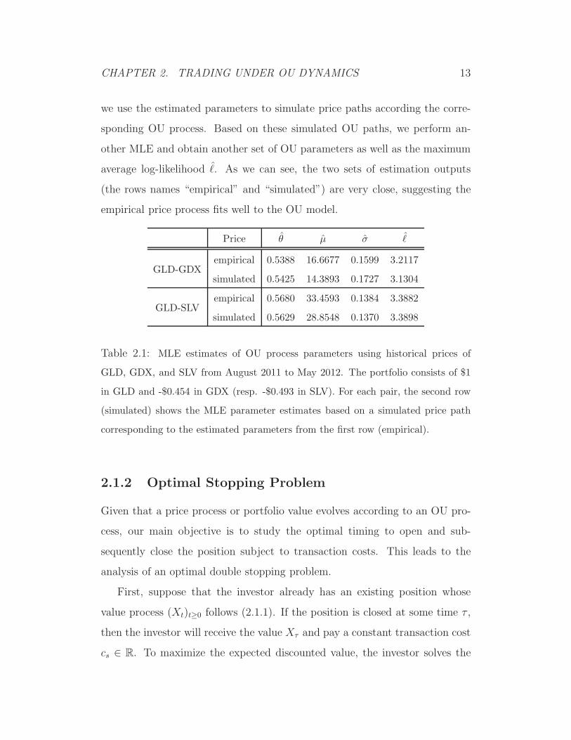
We summarize the estimation results in Table 2.1. For each pair, we first
estimate the parameters for the OU model from empirical price data. Then,
CHAPTER 2. TRADING UNDER OU DYNAMICS 13
we use the estimated parameters to simulate price paths according the corre-
sponding OU process. Based on these simulated OU paths, we perform an-
other MLE and obtain another set of OU parameters as well as the maximum
average log-likelihood ℓ. As we can see, the two sets of estimation outputs
(the rows names “empirical” and “simulated”) are very close, suggesting the
empirical price process fits well to the OU model.
Price θ µ σ ℓ
GLD-GDXempirical 0.5388 16.6677 0.1599 3.2117
simulated 0.5425 14.3893 0.1727 3.1304
GLD-SLVempirical 0.5680 33.4593 0.1384 3.3882
simulated 0.5629 28.8548 0.1370 3.3898
Table 2.1: MLE estimates of OU process parameters using historical prices of
GLD, GDX, and SLV from August 2011 to May 2012. The portfolio consists of $1
in GLD and -$0.454 in GDX (resp. -$0.493 in SLV). For each pair, the second row
(simulated) shows the MLE parameter estimates based on a simulated price path
corresponding to the estimated parameters from the first row (empirical).
2.1.2 Optimal Stopping Problem
Given that a price process or portfolio value evolves according to an OU pro-
cess, our main objective is to study the optimal timing to open and sub-
sequently close the position subject to transaction costs. This leads to the
analysis of an optimal double stopping problem.
First, suppose that the investor already has an existing position whose
value process (Xt)t≥0 follows (2.1.1). If the position is closed at some time τ ,
then the investor will receive the value Xτ and pay a constant transaction cost
cs ∈ R. To maximize the expected discounted value, the investor solves the
CHAPTER 2. TRADING UNDER OU DYNAMICS 14
optimal stopping problem
V (x) = supτ∈T
Ex
e−rτ (Xτ − cs)
, (2.1.2)
where T denotes the set of all F-stopping times, and r > 0 is the investor’s
subjective constant discount rate. We have also used the shorthand notation:
Ex· ≡ E·|X0 = x.From the investor’s viewpoint, V (x) represents the expected liquidation
value associated with X . On the other hand, the current price plus the trans-
action cost constitute the total cost to enter the trade. The investor can always
choose the optimal timing to start the trade, or not to enter at all. This leads
us to analyze the entry timing inherent in the trading problem. Precisely, we
solve
J(x) = supν∈T
Ex
e−rν(V (Xν)−Xν − cb)
, (2.1.3)
with r > 0, cb ∈ R. In other words, the investor seeks to maximize the
expected difference between the value function V (Xν) and the current Xν ,
minus transaction cost cb. The value function J(x) represents the maximum
expected value of the investment opportunity in the price process X , with
transaction costs cb and cs incurred, respectively, at entry and exit. For our
analysis, the pre-entry and post-entry discount rates, r and r, can be different,
as long as 0 < r ≤ r. Moreover, the transaction costs cb and cs can also differ,
as long as cs+ cb > 0. Furthermore, since τ = +∞ and ν = +∞ are candidate
stopping times for (2.1.2) and (2.1.3) respectively, the two value functions V (x)
and J(x) are non-negative.
As extension, we can incorporate a stop-loss level of the pairs trade, that
caps the maximum loss. In practice, the stop-loss level may be exogenously
imposed by the manager of a trading desk. In effect, if the price X ever reaches
level L prior to the investor’s voluntary liquidation time, then the position will
CHAPTER 2. TRADING UNDER OU DYNAMICS 15
be closed immediately. The stop-loss signal is given by the first passage time
τL := inft ≥ 0 : Xt ≤ L.
Therefore, we determine the entry and liquidation timing from the constrained
optimal stopping problem:
JL(x) = supν∈T
Ex
e−rν(VL(Xν)−Xν − cb)
, (2.1.4)
VL(x) = supτ∈T
Ex
e−r(τ∧τL)(Xτ∧τL − cs)
. (2.1.5)
Due to the additional timing constraint, the investor may be forced to exit
early at the stop-loss level for any given liquidation level. Hence, the stop-loss
constraint reduces the value functions, and precisely we deduce that x− cs ≤VL(x) ≤ V (x) and 0 ≤ JL(x) ≤ J(x). As we will show in Sections 2.3 and 2.4,
the optimal timing strategies with and without stop-loss are quite different.
2.2 Method of Solution
In this section, we disucss our method of solution. First, we denote the in-
finitesimal generator of the OU process X by
L =σ2
2
d2
dx2+ µ(θ − x)
d
dx, (2.2.1)
and recall the classical solutions of the differential equation
Lu(x) = ru(x), (2.2.2)
for x ∈ R, are (see e.g. p.542 of Borodin and Salminen [2002] and Prop. 2.1
of Alili et al. [2005]):
F (x) ≡ F (x; r) :=
∫ ∞
0
urµ−1e
√
2µ
σ2 (x−θ)u−u2
2 du, (2.2.3)
G(x) ≡ G(x; r) :=
∫ ∞
0
urµ−1e
√
2µ
σ2 (θ−x)u−u2
2 du. (2.2.4)
CHAPTER 2. TRADING UNDER OU DYNAMICS 16
Direct differentiation yields that F ′(x) > 0, F ′′(x) > 0, G′(x) < 0 and G′′(x) >
0. Hence, we observe that both F (x) and G(x) are strictly positive and convex,
and they are, respectively, strictly increasing and decreasing.
Define the first passage time of X to some level κ by τκ = inft ≥ 0 : Xt =
κ. As is well known, F and G admit the probabilistic expressions (see Ito
and McKean [1965] and Rogers and Williams [2000]):
Exe−rτκ =
F (x)F (κ)
if x ≤ κ,
G(x)G(κ)
if x ≥ κ.
A key step of our solution method involves the transformation
ψ(x) :=F
G(x). (2.2.5)
Starting at any x ∈ R, we denote by τa∧τb the exit time from an interval [a, b]
with −∞ ≤ a ≤ x ≤ b ≤ +∞. With the reward function h(x) = x − cs, we
compute the corresponding expected discounted reward:
Exe−r(τa∧τb)h(Xτa∧τb)
= h(a)Exe−rτa11τa<τb+ h(b)Exe−rτb11τa>τb (2.2.6)
= h(a)F (x)G(b)− F (b)G(x)
F (a)G(b)− F (b)G(a)+ h(b)
F (a)G(x)− F (x)G(a)
F (a)G(b)− F (b)G(a)(2.2.7)
= G(x)
[h(a)
G(a)
ψ(b)− ψ(x)
ψ(b)− ψ(a)+h(b)
G(b)
ψ(x)− ψ(a)
ψ(b)− ψ(a)
]
= G(ψ−1(z))
[
H(za)zb − z
zb − za+H(zb)
z − zazb − za
]
, (2.2.8)
where za = ψ(a), zb = ψ(b), and
H(z) :=
hG ψ−1(z) if z > 0,
limx→−∞
(h(x))+
G(x)if z = 0.
(2.2.9)
The second equality (2.2.7) follows from the fact that f(x) := Exe−r(τa∧τb)11τa<τbis the unique solution to (2.2.2) with boundary conditions f(a) = 1 and f(b) =
CHAPTER 2. TRADING UNDER OU DYNAMICS 17
0. Similar reasoning applies to the function g(x) := Exe−r(τa∧τb)11τa>τb with
g(a) = 0 and g(b) = 1. The last equality (2.2.8) transforms the problem from
x coordinate to z = ψ(x) coordinate (see (2.2.5)).
The candidate optimal exit interval [a∗, b∗] is determined by maximizing
the expectation in (2.2.6). This is equivalent to maximizing (2.2.8) over za
and zb in the transformed problem. This leads to
W (z) := supza,zb:za≤z≤zb
[
H(za)zb − z
zb − za+H(zb)
z − zazb − za
]
. (2.2.10)
This is the smallest concave majorant of H . Applying the definition of W to
(2.2.8), we can express the maximal expected discounted reward as
G(x)W (ψ(x)) = supa,b:a≤x≤b
Exe−r(τa∧τb)h(Xτa∧τb).
Remark 2.2.1. If a = −∞, then we have τa = +∞ and 11τa<τb = 0 a.s.
In effect, this removes the lower exit level, and the corresponding expected
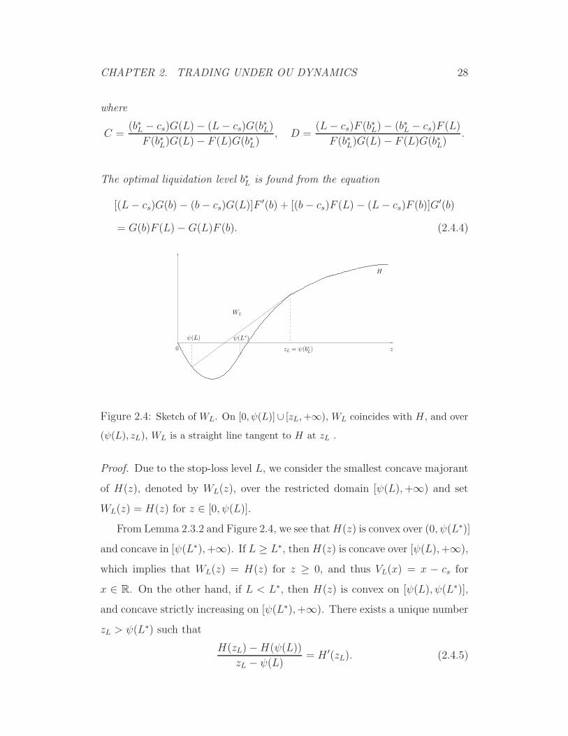
where the last equality follows from the fact that (L− r)V (x) = 0 for x < b∗,
since W is a straight line for z ≤ ψ(b∗), and b < L∗ < b∗. Hence, for z ∈(0, ψ(b)), Hδ′′(z) ≤ H ′′(z) ≤ 0 and Hδ(z) is also concave.
Since V (x) ≥ V δ(x) ≥ 0, we have H(z) ≥ Hδ(z) for z ∈ (0,+∞). Con-
sidering H(0) = Hδ(0) = 0 and H(0+), Hδ(0+) > 0, we have H ′(0+) ≥Hδ′(0+) ≥ 0. This, along with Hδ′′(z) ≤ H ′′(z) ≤ 0 for z ∈ (0, ψ(b)), imply
that H ′(z) ≥ Hδ′(z) for z ∈ (0, ψ(b)). So Hδ′(z) ≤ H ′(z) = 0. Considering
Hδ′(zδ) = 0 and the concavity of Hδ, we conclude that zδ ≤ z, which by the
monotonicity of ψ is equivalent to dδ ≤ d∗.
To show Jδ(x) ≤ J(x), it is equivalent to establish W δ(z) ≤ W (z) for all
z ∈ [0,∞): (i) For z ∈ [0, zδ], this holds since W δ(z) = Hδ(z), W (z) = H(z),
and Hδ(z) ≤ H(z). (ii) For z ∈ (zδ, z], W δ(z) = Hδ(zδ) ≤ H(zδ) ≤ H(z) =
W (z), where the last inequality follows from the fact that H ′(z) ≥ 0 for
z ∈ (zδ, z]. (iii) For z ∈ (z,+∞), W δ(z) = Hδ(zδ) ≤ H(z) = W (z).
This means that the minimum holding period leads to a lower optimal
entry level and lower value function as compared to the original value function
J in (2.1.3).
2.5.2 Path-Dependent Risk Penalty
In addition to maximizing the expected liquidation value, a risk-sensitive in-
vestor may be concerned about the price fluctuation over time, and therefore,
be willing to adjust her liquidation timing depending on the path behavior of
prices. This motivates the incorporation of a path-dependent risk penalty up
to the liquidation time τ . To illustrate this idea, we apply a penalty term of
the form Ex∫ τ
0e−ruq(Xu) du, where q(x) could be any positive penalty func-
tion. This risk penalty only applies when the investor is holding the position,
but not before entry. Hence, the investor solves the penalized optimal timing
CHAPTER 2. TRADING UNDER OU DYNAMICS 41
problems:
J q(x) = supν∈T
Ex
e−rτ (Vq(Xν)−Xν − cb)
,
Vq(x) = supτ∈T
Ex
e−rτ (Xτ − cs)−∫ τ
0
e−ruq(Xu) du
. (2.5.3)
As a special case, let q(x) ≡ q, a strictly positive constant. Then, by
computing the integral in (2.5.3),
Vq(x) = supτ∈T
E
e−rτ (Xτ − (cs −q
r))
− q
r. (2.5.4)
This presents an interesting connection between the penalized problem Vq(x)in (2.5.4) and the unpenalized optimal stopping problem V in (2.1.2). Indeed,
we observe that the penalty term amounts to reducing the transaction cost
cs by the positive constant q
r. In other words, the optimal stopping time τ ∗q
for Vq(x) is identical to the optimal stopping time τ ∗ for V (x) in (2.1.2) but
with cs replaced by cs − q
r. Furthermore, since b∗ is increasing in cs, a higher
penalty q lowers the optimal liquidation level. As for the entry problem J q,
the solution is found from Theorem 2.3.7 by modifying the transaction cost to
be cb+q
r. More sophisticated path-dependent risk penalties can be considered
under this formulation, including those based on the (integrated) shortfall with
q(x) = ρ((m − x)+) where m is a constant benchmark and ρ is an increasing
convex loss function (see e.g. [Follmer and Schied, 2004, Chap 4.9]).
CHAPTER 3. TRADING UNDER EXPONENTIAL OU DYNAMICS 42
Chapter 3
Trading under Exponential OU
Dynamics
In this chapter, we solve an optimal double stopping problem to determine
the optimal times to enter and subsequently exit the market, when prices are
driven by an exponential Ornstein-Uhlenbeck process. In addition, we ana-
lyze a related optimal switching problem that involves an infinite sequence
of trades, and identify the conditions under which the double stopping and
switching problems admit the same optimal entry and/or exit timing strate-
gies. Among our results, we find that the investor generally enters when the
price is low, but may find it optimal to wait if the current price is sufficiently
close to zero. In other words, the continuation (waiting) region for entry is
disconnected. Numerical results are provided to illustrate the dependence of
timing strategies on model parameters and transaction costs.
In Section 3.1, we formulate both the optimal double stopping and optimal
switching problems. Then, we present our analytical and numerical results in
Section 3.2. The proofs of our main results are detailed in Section 3.3. Finally,
Appendix C contains the proofs for a number of lemmas.
CHAPTER 3. TRADING UNDER EXPONENTIAL OU DYNAMICS 43
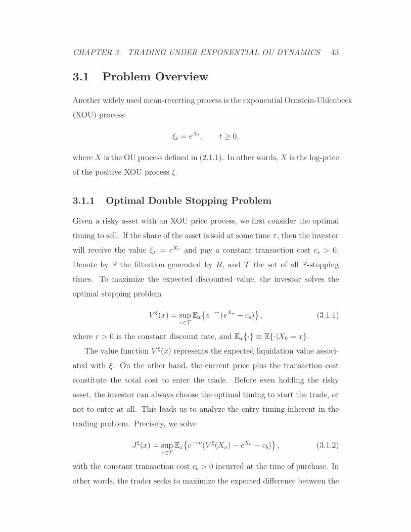
3.1 Problem Overview
Another widely used mean-reverting process is the exponential Ornstein-Uhlenbeck
(XOU) process:
ξt = eXt , t ≥ 0,
where X is the OU process defined in (2.1.1). In other words, X is the log-price
of the positive XOU process ξ.
3.1.1 Optimal Double Stopping Problem
Given a risky asset with an XOU price process, we first consider the optimal
timing to sell. If the share of the asset is sold at some time τ , then the investor
will receive the value ξτ = eXτ and pay a constant transaction cost cs > 0.
Denote by F the filtration generated by B, and T the set of all F-stopping
times. To maximize the expected discounted value, the investor solves the
optimal stopping problem
V ξ(x) = supτ∈T
Ex
e−rτ (eXτ − cs)
, (3.1.1)
where r > 0 is the constant discount rate, and Ex· ≡ E·|X0 = x.The value function V ξ(x) represents the expected liquidation value associ-
ated with ξ. On the other hand, the current price plus the transaction cost
constitute the total cost to enter the trade. Before even holding the risky
asset, the investor can always choose the optimal timing to start the trade, or
not to enter at all. This leads us to analyze the entry timing inherent in the
trading problem. Precisely, we solve
Jξ(x) = supν∈T
Ex
e−rν(V ξ(Xν)− eXν − cb)
, (3.1.2)
with the constant transaction cost cb > 0 incurred at the time of purchase. In
other words, the trader seeks to maximize the expected difference between the
CHAPTER 3. TRADING UNDER EXPONENTIAL OU DYNAMICS 44
value function V ξ(Xν) and the current eXν , minus transaction cost cb. The
value function Jξ(x) represents the maximum expected value of the investment
opportunity in the price process ξ, with transaction costs cb and cs incurred,
respectively, at entry and exit. For our analysis, the transaction costs cb and
cs can be different. To facilitate presentation, we denote the functions
hξs(x) = ex − cs and hξb(x) = ex + cb. (3.1.3)
If it turns out that Jξ(X0) ≤ 0 for some initial value X0, then the investor
will not start to trade X (see Appendix A below). In view of the example
in Appendix A, it is important to identify the trivial cases under any given
dynamics. Under the XOU model, since supx∈R(Vξ(x) − hξb(x)) ≤ 0 implies
that Jξ(x) ≤ 0 for x ∈ R, we shall therefore focus on the case with
supx∈R
(V ξ(x)− hξb(x)) > 0, (3.1.4)
and solve for the non-trivial optimal timing strategy.
3.1.2 Optimal Switching Problem
Under the optimal switching approach, the investor is assumed to commit to
an infinite number of trades. The sequential trading times are modeled by the
stopping times ν1, τ1, ν2, τ2, · · · ∈ T such that
0 ≤ ν1 ≤ τ1 ≤ ν2 ≤ τ2 ≤ . . . .
A share of the risky asset is bought and sold, respectively, at times νi and τi,
i ∈ N. The investor’s optimal timing to trade would depend on the initial
position. Precisely, under the XOU model, if the investor starts with a zero
position, then the first trading decision is when to buy and the corresponding
optimal switching problem is
Jξ(x) = supΛ0
Ex
∞∑
n=1
[e−rτnhξs(Xτn)− e−rνnhξb(Xνn)]
, (3.1.5)
CHAPTER 3. TRADING UNDER EXPONENTIAL OU DYNAMICS 45
with the set of admissible stopping times Λ0 = (ν1, τ1, ν2, τ2, . . . ), and the
reward functions hξs and hξb defined in (3.1.3). On the other hand, if the investor
is initially holding a share of the asset, then the investor first determines when
to sell and solves
V ξ(x) = supΛ1
Ex
e−rτ1hξs(Xτ1) +∞∑
n=2
[e−rτnhξs(Xτn)− e−rνnhξb(Xνn)]
, (3.1.6)
with Λ1 = (τ1, ν2, τ2, ν3, . . . ).
In summary, the optimal double stopping and switching problems differ in
the number of trades. Observe that any strategy for the double stopping prob-
lems (3.1.1) and (3.1.2) are also candidate strategies for the switching problems
(3.1.6) and (3.1.5) respectively. Therefore, it follows that V ξ(x) ≤ V ξ(x) and
Jξ(x) ≤ Jξ(x). Our objective is to derive and compare the corresponding
optimal timing strategies under these two approaches.
3.2 Summary of Analytical Results
We first summarize our analytical results and illustrate the optimal trading
strategies. The method of solutions and their proofs will be discussed in Sec-
tion 3.3. We begin with the optimal stopping problems (3.1.1) and (3.1.2)
under the XOU model.
3.2.1 Optimal Double Stopping Problem
We now present the result for the optimal exit timing problem under the XOU
model. First, we obtain a bound for the value function V ξ.
Lemma 3.2.1. There exists a positive constant Kξ such that, for all x ∈ R,
0 ≤ V ξ(x) ≤ ex +Kξ.
CHAPTER 3. TRADING UNDER EXPONENTIAL OU DYNAMICS 46
Theorem 3.2.2. The optimal liquidation problem (3.1.1) admits the solution
V ξ(x) =
ebξ∗
−csF (bξ∗)
F (x) if x < bξ∗,
ex − cs if x ≥ bξ∗,
(3.2.1)
where the optimal log-price level bξ∗ for liquidation is uniquely found from the
Indeed, this is the approach used by Zervos et al. [2013] for checking the solu-
tions of their optimal switching problems.
4.2.3 Numerical Examples
We numerically implement Theorems 4.2.2, 4.2.4, and 4.2.7, and illustrate the
associated starting and stopping thresholds. In Figure 4.1 (left), we observe
the changes in optimal starting and stopping levels as speed of mean reversion
increases. Both starting levels dχ∗ and dχ∗ rise with µ, from 0.0964 to 0.1219
and from 0.1460 to 0.1696, respectively, as µ increases from 0.3 to 0.85. The
optimal switching stopping level bχ∗ also increases. On the other hand, stop-
ping level bχ∗ for the starting-stopping problem stays relatively constant as µ
changes.
In Figure 4.1 (right), we see that as the stopping cost cs increases, the
increase in the optimal stopping levels is accompanied by a fall in optimal
starting levels. In particular, the stopping levels, bχ∗ and bχ∗ increase. In
comparison, both starting levels dχ∗ and dχ∗ fall. The lower starting level and
higher stopping level mean that the entry and exit times are both delayed as a
result of a higher transaction cost. Interestingly, although the cost cs applies
only when the process is stopped, it also has an impact on the timing to start,
as seen in the changes in dχ∗ and dχ∗ in the figure.
In Figure 4.1, we can see that the continuation (waiting) region of the
switching problem (dχ∗, bχ∗) lies within that of the starting-stopping problem
(dχ∗, bχ∗). The ability to enter and exit multiple times means it is possible to
earn a smaller reward on each individual start-stop sequence while maximizing
aggregate return. Moreover, we observe that optimal entry and exit levels of
the starting-stopping problem is less sensitive to changes in model parameters
than the entry and exit thresholds of the switching problem.
Figure 4.2 shows a simulated CIR path along with optimal entry and exit
CHAPTER 4. TRADING UNDER CIR DYNAMICS 81
levels for both starting-stopping and switching problems. Under the starting-
stopping problem, it is optimal to start once the process reaches dχ∗ = 0.0373
and to stop when the process hits bχ∗ = 0.4316. For the switching problem, it
is optimal to start once the process values hits dχ∗ = 0.1189 and to stop when
the value of the CIR process rises to bχ∗ = 0.2078. We note that both stopping
levels bχ∗ and bχ∗ are higher than the long-run mean θ = 0.2, and the starting
levels dχ∗ and dχ∗ are lower than θ. The process starts at Y0 = 0.15 > dχ∗,
under the optimal switching setting, the first time to enter occurs on day 8
when the process falls to 0.1172 and subsequently exits on day 935 at a level
of 0.2105. For the starting-stopping problem, entry takes place much later on
day 200 when the process hits 0.0306 and exits on day 2671 at 0.4369. Under
the optimal switching problem, two entries and two exits will be completed
by the time a single entry-exit sequence is realized for the starting-stopping
problem.
0.3 0.4 0.5 0.6 0.7 0.80.05
0.1
0.15
0.2
0.25
0.3
µ
dχ∗
bχ∗
dχ∗
bχ∗
0.01 0.02 0.03 0.04 0.050.1
0.15
0.2
0.25
cs
dχ∗
bχ∗
dχ∗
bχ∗
Figure 4.1: (Left) The optimal starting and stopping levels vs speed of mean rever-
sion µ. Parameters: σ = 0.15, θ = 0.2, r = 0.05, cs = 0.001, cb = 0.001. (Right) The
optimal starting and stopping levels vs transaction cost cs. Parameters: µ = 0.6,
σ = 0.15, θ = 0.2, r = 0.05, cb = 0.001.
CHAPTER 4. TRADING UNDER CIR DYNAMICS 82
0 1000 2000 3000 4000 50000
0.1
0.2
0.3
0.4
0.5
0.6
0.7
0.8
Days
bχ∗
b∗
d∗
dχ∗
Figure 4.2: A sample CIR path, along with starting and stopping levels. Under
the starting-stopping setting, a starting decision is made at νdχ∗ = inft ≥ 0 : Yt ≤dχ∗ = 0.0373, and a stopping decision is made at τbχ∗ = inft ≥ νdχ∗ : Yt ≥bχ∗ = 0.4316. Under the optimal switching problem, entry and exit take place at
for every x ∈ R and every τ ∈ T . Hence, J(x) ≤ KG(x). Since τ = +∞ is a
candidate stopping time, we have J(x) ≥ 0.
APPENDIX B. APPENDIX FOR CHAPTER 2 104
B.4 Proof of Lemma 2.3.6 (Properties of H)
We first show that V (x) and h(x) are twice differentiable everywhere, except
for x = b∗. Recall that
V (x) =
(b∗ − cs)F (x)F (b∗)
if x ∈ (−∞, b∗),
x− cs otherwise,
and h(x) = V (x)− x− cb.
Therefore, it follows from (2.3.3) that
V ′(x) =
(b∗ − cs)F ′(x)F (b∗)
= F ′(x)F ′(b∗)
if x ∈ (−∞, b∗),
1 if x ∈ (b∗,+∞),
which implies that V ′(b∗−) = 1 = V ′(b∗+). Therefore, V (x) is differentiable
everywhere and so is h. However, V (x) is not twice differentiable since
V ′′(x) =
F ′′(x)F ′(b∗)
if x ∈ (−∞, b∗),
0 if x ∈ (b∗,+∞),
and V ′′(b∗−) 6= V ′′(b∗+). Consequently, h(x) = V (x) − x − cb is not twice
differentiable at b∗.
The twice differentiability of G and ψ are straightforward. The continuity
and differentiability of H on (0,+∞) and twice differentiability on (0, ψ(b∗))∪(ψ(b∗),+∞) follow directly. Observing that h(x) > 0 as x → −∞, H is also
continuous at 0 by definition. We now establish the properties of H.
(i) First we prove the value of H at 0:
H(0) = limx→−∞
(h(x))+
G(x)= lim sup
x→−∞
(b∗−cs)F (b∗)
F (x)− x− cb
G(x)
= lim supx→−∞
(b∗−cs)F (b∗)
F ′(x)− 1
G′(x)= 0.
Next, observe that limx→−∞ h(x) = +∞ and h(x) = −(cs + cb), for x ∈[b∗,+∞). Since F ′(x) is strictly increasing and F ′(x) > 0 for x ∈ R, we have,
APPENDIX B. APPENDIX FOR CHAPTER 2 105
for x < b∗,
h′(x) = V ′(x)− 1 =F ′(x)
F ′(b∗)− 1 <
F ′(b∗)
F ′(b∗)− 1 = 0,
which implies that h(x) is strictly decreasing for x ∈ (−∞, b∗). Therefore,
there exists a unique solution d to h(x) = 0, and d < b∗, such that h(x) > 0
if x ∈ (−∞, d) and h(x) < 0 if x ∈ (d,+∞). It is trivial that ψ(x) ∈ (0,+∞)
for x ∈ R and is a strictly increasing function. Therefore, along with the fact
that G(x) > 0, property (i) follows directly.
(ii) With z = ψ(x), for x > b∗,
H ′(z) =1
ψ′(x)(h
G)′(x) =
1
ψ′(x)(−(cs + cb)
G(x))′ =
1
ψ′(x)
(cs + cb)G′(x)
G2(x)< 0,
since ψ′(x) > 0, G′(x) < 0, and G2(x) > 0. Therefore, H(z) is strictly
decreasing for z > ψ(b∗).
(iii) By the definition of H ,
H ′′(z) =2
σ2G(x)(ψ′(x))2(L− r)h(x), z = ψ(x).
Since σ2, G(x) and (ψ′(x))2 are all positive, we only need to determine the
Since µ, r > 0 by assumption, (Lχ − r)hχ(y) is strictly increasing on (0, bχ∗).
Next, we show that 0< yb < ys < bχ∗. By the fact that F χ′(0) = rµθ
and the
assumption that V χ(0) = bχ∗−csFχ(bχ∗)
> cb, we have
V χ′(0) =bχ∗ − csF χ(bχ∗)
F χ′(0) =bχ∗ − csF χ(bχ∗)
r
µθ>rcbµθ.
In addition, by the convexity of V χ and V χ′(bχ∗) = 1, it follows that
rcbµθ
< V χ′(0) < V χ′(bχ∗) = 1,
which implies µθ > rcb and hence yb > 0. By simply comparing the definitions
of yb and ys, it is clear that yb < ys. Therefore, by observing that (Lχ −r)hχ(yb) = 0, we conclude (Lχ−r)hχ(y) < 0 if y ∈ [0, yb), and (Lχ−r)hχ(y) > 0
if y ∈ (yb,+∞). This suggests the concavity and convexity of Hχ as desired.