Page 1
Page1
OptimalPowerFlowPaper8
StaffpaperbyMehrdadPirniaRichardO’NeillPaulaLipkaClayCampaigne
June2013TheviewspresentedarethepersonalviewsoftheauthorsandnottheFederalEnergyRegulatoryCommissionoranyofitsCommissioners.
Page 2
Page2
AComputationalStudyofLinearApproximationstotheConvexConstraintsintheIterativeLinearIV‐ACOPFFormulation
MehrdadPirnia,RichardO’Neill,PaulaLipka,ClayCampaigne
[email protected] ;[email protected] ;[email protected] ;[email protected]
June2013
AbstractandExecutiveSummaryInthispaper,wetesttheeffectofpreprocessedanditerativelinearcutsontheconvexconstraintsmaximumvoltageandmaximumcurrent initerativelinearapproximationofthecurrentvoltageIV formulationoftheACOPF ILIV‐ACOPF problem.ThenonconvexconstraintsarelinearizedusingiterativefirstorderTaylorseriesapproximation.TheILIV‐ACOPFissolvedasasinglelinearprogramorasequenceoflinearprograms.TheILIV‐ACOPFmodelistestedonthe14‐bus,30‐bus,57‐busand118‐busIEEEtestsystems.TheexecutiontimeandthequalityofthesolutionobtainedfromtheILIV‐ACOPFarecomparedfordifferenttestsystemsandbenchmarkedagainsttheequivalentnonlinearACOPFformulation.Theresultsshowexecutiontimeupto8timesfasterandsolutionsclosetothenonlinearsolver.Theperformanceofdifferentalgorithmicparametersvariesdependingonthetestproblem.Asthenumberofpreprocessedcutsforeachbusandlineincreases,therelativeerrordecreases.Theresultsindicatethat16to32constraintsarethebestnumberofpreprocessedconstraintsinatradeoffbetweenaccuracyandsolutiontime.Themarginalvalueofmorethan32andmaybe16preprocessedconstraintsinthissettingisnegative.Nevertheless,thenumberofpreprocessedconstraintscanbesetbasedontheperformanceandrequirementsofthespecificproblembeingsolved.Usingiterativecutsoftenresultsinfasterconvergencetoafeasiblesolution.Whensolvingwithoutusingiterativecuts,thesolutioniswithin18%ofthebest‐knownnonlinearfeasiblesolution;withiterativecuts,thesolutioniswithin2.5%ofthebest‐knownnonlinearsolution.At16or32preprocessedconstraints,solutiontimeisuptoabout8timesfasterthanthenonlinearsolver IPOPT .Disclaimer:TheviewspresentedarethepersonalviewsoftheauthorsandnottheFederalEnergyRegulatoryCommissionoranyofitsCommissioners.
Page 3
Page3
TableofContents
1.Introduction 42.Nomenclature 53.Formulations 64.LinearApproximations 75.ComputationalResults 96.Conclusion 15References 16
Page 4
Page4
1.Introduction
SinceCarpentier 1962 introducedACoptimalpowerflow ACOPF problem,theACOPFhasreceivedconsiderableattention.Itisattheheartofpowersystemefficiency.TheACOPFoptimizesthesteadystateperformanceofanACpowersystembyminimizinganobjectivefunctionsuchasgenerationcostormaximizingmarketsurpluswhilesatisfyingsystemconstraintsincludingnodalrealpowerbalance,nodalreactivepowerbalance,boundsonbusvoltages,boundsontransmissionlinesflow,boundsonrealandreactivepowerinjections,andsystemcontingencies.SincetheACOPF’sintroduction,differentobjectivefunctionsandformulationshavebeentried seeCainetal .ThecanonicalACOPFproblemusesrealandreactivepowerinjectionsandthepolarrepresentationofvoltageforthenetworkequations.ACOPFproblemshavenonconvexcontinuousfunctionsandcanbelarge.Moredifficultvariationsincludebinaryvariablesfortopologycontrolandunitcommitment see,forexample,PotluriandHedman .
SolvinganACOPFproblemthatmeetspowersystem’sphysicalcriteriahascontinuedtobeachallengeinpowersystemoperations.WhilemostNLPsolversfindlocaloptimalsolutionsmostofthetime,theirlengthysolutiontimesandpoorconvergence especiallywiththeintroductionofbinaryvariables havefocusedattentiononlinearapproximations.Linearprogramming LP methodsplayasignificantroleinsolvingtheseproblemswithmorerobustsolutionsandbetterexecutiontimes.Onecommonlinearprogramapproachisthedistributionfactormodel.Inanotherlinearprogramapproach,therealpartoftheadmittancematrixisconsiderednegligible,reactivepowerandvoltagemagnitudearedroppedfromtheformulation,andbusvoltageanglesareassumedtobenear‐zero Stott,etal.,2009 .
AvastbodyofliteratureproposesdifferentoptimizationmethodstosolvetheACOPFincludingLagrangianapproaches,sequentialquadraticprogramming,sequentiallinearprogramming,interiorpointmethods,andheuristics.Literaturereviewsappearperiodically see,forexample,DommelandTinney,HuneaultandGaliana,Momoh,etal,FrankandSteponaviceandCastilloandO’Neill,2013a).TheliteraturereviewspresentanevolutionofapproachestosolvetheACOPF.Capitanescuetal(2011)reviewsthestateoftheartandchallengestotheoptimalpowerflowcomputationsincludingcorrectivepost‐contingencyactions,voltageandtransientstabilityconstraints,problemsizereduction,discretevariablesanduncertainty.
O’Neillelal(2012a)formulatetheACOPFinseveralways,compareeachformulation’sproperties,andarguethattherectangularcurrent‐voltageor“IV”formulationanditslinearapproximationsmaybeeasiertosolvethanthetraditionalquadraticpowerflow“PQV”formulation.O’Neilletal(2012b)comparesolvingtheIVlinearapproximationoftheACOPFtosolvingtheACOPFwithseveralnonlinearsolvers.Ingeneral,thelinearapproximationapproachismorerobustandfasterthanseveralofthecommercialnonlinearsolvers.Onseveralstartingpoints,thenonlinearsolversfailedtoconvergeorcontainedpositiverelaxationvariablesabovethethreshold.Theiterativelinearprogramapproachfindsanear‐feasiblenear‐optimalinalmostallproblemsandstartingpoints.CastilloandO’Neill(2013b)presentanexperimentalframework,statisticalmethodsandnumericalresultsfromtestingcommercialnonlinearsolverswithseveralACOPFformulationsandinitializations.Theexperimentsindicateaclearadvantagetoemployingarectangularformulationoverapolarformulationandusingmultiplesolvers.
Page 5
Page5
Inspiteofalltheworkthathasbeendone,theACOPFremains‘verymuchaworkinprogress’ StottandAlsaç,2012 .Further,theystatethatsolutionstotheproblemsencounteredin‘real‐life’are‘noteasytoobtain’andstillrequiresignificantindividualinterventionandtuning.
Inthispaper,wetesttheiterativelinearization IL approachtotheIVACOPFformulation,proposedin O'Neill,etal.,2012 onfourIEEEstandardtestproblems 14‐bus,30‐bus,57‐busand118‐bustestsystems withlinecurrentconstraintsadded.Wevarythenumberofpreprocessedlinearcuts,toapproximatetheconvexquadraticvoltageandcurrentconstraintswithandwithoutiterativeconstraints.Wereportthesolutiontimeandaccuracy.
Therestofthepaperisorganizedasfollows.Section2presentsthenotationtobeusedinfollowingsections.Section3presentsabriefreviewoftheIV‐ACOPFandILIV‐ACOPFformulations.Section4presentsanddiscussesthelinearapproximationtechniques,suchaspre‐processedcuts,iterativecutsandnon‐convexconstraintlinearizations,whichareusedtoapproximatetheIV‐ACOPFformulation.Section5presentsnumericalresultsforthetestsystemsshowingtheperformanceofthismethodcomparedtothenonlinearOPFproblem.Finally,Section6highlightsthemainconclusionsandcontributionsofthepaper.Theappendixcontainsthenumericalresults.2.NotationIndicesandSetsn,m arebus node indices;n,mϵ 1,…,N where Nisthenumberofbuses.k isatransmissionelement.kϵ 1,…,K where Kisthenumberoftransmissionelements.Each
khasapairofterminalbusesnandm.r realpartofthecomplexnumberorvariable superscriptj imaginarypartofthecomplexnumberorvariable superscriptj is ‐1 1/2s istheindexofthepreprocessedconstraintswhere sϵ S 0,1,…,S‐1 .h indexesamajoriteration solvingalinearprogram ofthealgorithmVariablespn istherealpowerinjection positive orwithdrawal negative atbus nqn isthereactivepowerinjectionorwithdrawalatbus nvrn realpartofthevoltageatbusnvjn imaginarypartofthevoltageatbusnvn isthevoltagemagnitudeatbusn.vn vrn 2 vjn 2 1/2
irn realpartofthecurrentatbusnijn imaginarypartofthecurrentatbusnin isthecurrentmagnitudeatbus nwherein irn 2 ijn 2 1/2
irnmk realpartofthecurrentfrombusn tobusm onlinekijnmk imaginarypartofthecurrentfrombusn tobusm onlinekinmk isthecurrentmagnitudeintokatbus n tobusm ;inmk irnmk 2 ijnmk 2 1/2 thecomplexvectorofbusvoltages; thecomplexvectorofbuscurrentinjections, thevectorofrealpowerinjections thevectorofreactivepowerinjections
Page 6
Page6
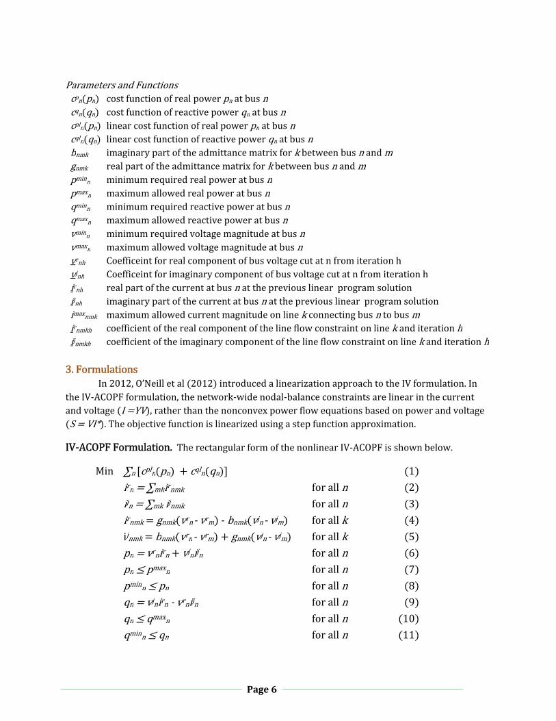
ParametersandFunctionscpn pn costfunctionofrealpowerpn atbusncqn qn costfunctionofreactivepowerqn atbusncpln pn linearcostfunctionofrealpowerpn atbusncqln qn linearcostfunctionofreactivepowerqn atbusnbnmk imaginarypartoftheadmittancematrixfork betweenbusnandmgnmk realpartoftheadmittancematrixfork betweenbusnandmpminn minimumrequiredrealpoweratbusnpmaxn maximumallowedrealpoweratbusnqminn minimumrequiredreactivepoweratbusnqmaxn maximumallowedreactivepoweratbusnvminn minimumrequiredvoltagemagnitudeatbusnvmaxn maximumallowedvoltagemagnitudeatbusnvrnh Coefficeintforrealcomponentofbusvoltagecutatnfromiterationhvjnh Coefficeintforimaginarycomponentofbusvoltagecutatnfromiterationhirnh realpartofthecurrentatbusn atthepreviouslinearprogramsolutionijnh imaginarypartofthecurrentatbusn atthepreviouslinearprogramsolutionimaxnmk maximumallowedcurrentmagnitudeonlinekconnectingbusn tobusmirnmkh coefficientoftherealcomponentofthelineflow constraint onlinekanditeration hijnmkh coefficientoftheimaginarycomponentofthelineflow constraint onlinekanditeration h3.Formulations
In2012,O’Neilletal 2012 introducedalinearizationapproachtotheIVformulation.IntheIV‐ACOPFformulation,thenetwork‐widenodal‐balanceconstraintsarelinearinthecurrentandvoltage I YV ,ratherthanthenonconvexpowerflowequationsbasedonpowerandvoltageS VI* .Theobjectivefunctionislinearizedusingastepfunctionapproximation.
IV‐ACOPFFormulation.TherectangularformofthenonlinearIV‐ACOPFisshownbelow.
Min ∑n cpln pn cqln qn 1
irn ∑mkirnmk foralln 2
ijn ∑mkijnmk foralln 3
irnmk gnmk vrn‐vrm ‐ bnmk vjn ‐ vjm forallk 4
ijnmk bnmk vrn‐vrm gnmk vjn ‐ vjm forallk 5
pn vrnirn vjnijn foralln 6
pn pmaxn foralln 7
pminn pn foralln 8
qn vjnirn‐vrnijn foralln 9
qn qmaxn foralln 10
qminn qn foralln 11
Page 7
Page7
vrn 2 vjn 2 vmaxn 2 foralln 12
vminn 2 vrn 2 vjn 2 foralln 13
irnmk 2 ijnmk 2 imaxnmk 2 forallk 14
TheaboveIV‐ACOPFformulationhas6Nvariablesas P,Q,Vr,Vj,Ir,Ij .Asshownin 2 ‐ 5 ,thecurrentflowequationsarelinear.Theseequationsreplacethequadraticortrigonometricformsofthepowerflowequations rectangularandpolarforms intraditionalACOPFmodels.Inthisformulation,realpowerequation 6 andreactivepowerequation 9 arequadraticnonconvexfunctionsofcurrentandvoltagewithbounds 7 , 8 , 10 ,and 11 .Maximumbusvoltagemagnitudeandcurrentflowlimits 12 and 14 arequadraticconvexconstraints.Theminimumvoltagemagnitudeconstraintisanonconvexquadraticconstraint 13 .
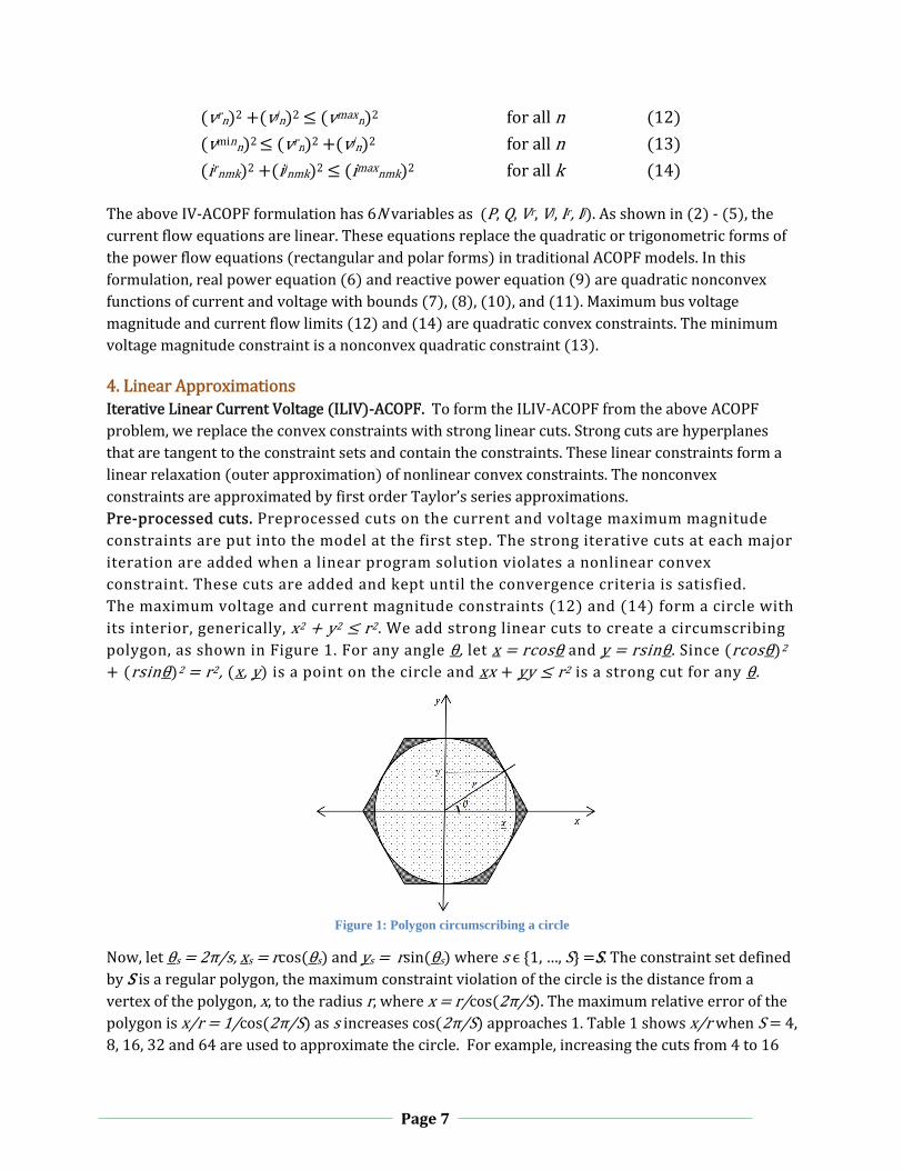
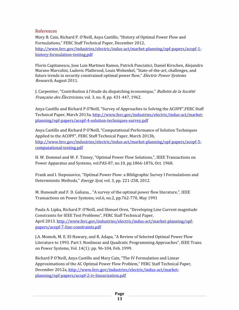
4.LinearApproximationsIterativeLinearCurrentVoltage ILIV ‐ACOPF.ToformtheILIV‐ACOPFfromtheaboveACOPFproblem,wereplacetheconvexconstraintswithstronglinearcuts.Strongcutsarehyperplanesthataretangenttotheconstraintsetsandcontaintheconstraints.Theselinearconstraintsformalinearrelaxation outerapproximation ofnonlinearconvexconstraints.ThenonconvexconstraintsareapproximatedbyfirstorderTaylor’sseriesapproximations.Pre‐processedcuts.Preprocessedcutsonthecurrentandvoltagemaximummagnitudeconstraintsareputintothemodelatthefirststep.Thestrongiterativecutsateachmajoriterationareaddedwhenalinearprogramsolutionviolatesanonlinearconvexconstraint.Thesecutsareaddedandkeptuntiltheconvergencecriteriaissatisfied.Themaximumvoltageandcurrentmagnitudeconstraints 12 and 14 formacirclewithitsinterior,generically,x2 y2 r2.Weaddstronglinearcutstocreateacircumscribingpolygon,asshowninFigure1.Foranyangleθ,letx rcosθandy rsinθ.Since rcosθ 2 rsinθ 2 r2, x,y isapointonthecircleandxx yy r2isastrongcutforanyθ.
Figure 1: Polygon circumscribing a circle
Now,letθs 2π/s,xs rcos θs andys rsin θs wheresϵ 1,…,S S.TheconstraintsetdefinedbySisaregularpolygon,themaximumconstraintviolationofthecircleisthedistancefromavertexofthepolygon,x,totheradiusr,wherex r/cos 2π/S .Themaximumrelativeerrorofthepolygonisx/r 1/cos 2π/S assincreasescos 2π/S approaches1.Table1showsx/rwhenS 4,8,16,32and64areusedtoapproximatethecircle.Forexample,increasingthecutsfrom4to16
Page 8
Page8
cutsincreasestheratiox/rfrom1.41to1.02.Adding32cutsprovidesacloseapproximationtotheactualfeasibleareaoftheconvexconstraints.
Table1:MaximumrelativeerrorNumber of linear cuts
Angle in radians (π/n)
Cos (angle) 1/ Cos (angle)
4 0.785 0.707 1.414 8 0.393 0.924 1.082 16 0.196 0.981 1.020 32 0.098 0.995 1.005 64 0.049 0.999 1.001
Iterativecuts.Letxh,yhbeasolutionatthemajoriterationh.Ifxh,yhviolatesamaximummagnitudeconstraint,thatis,zh2 xh2 yh2 r2.Leta r/zh,x axhandy ayh,then
x2 y2 axh 2 ayh 2 a2 xh2 yh2 a2 zh2 r2
Forvoltageconstraints,x,yandrarereplacedwithvrnh,vjnhandvmaxn.Forthecurrentconstraintsx,yandrarereplacedwithirnmh,irnmhandimaxnmk.Thesenewiterativeconstraintsreducethefeasibleareaandmakethecurrentoptimalsolutioninfeasible.Ateachiteration,theiterativeconstraintsareadded:
vrnhvrn vjnhvjn vmaxn 2
irnmkhirnmk ijnmkhijnmk imaxnmk 2
Theminimumvoltageconstraintisaddressedbyanactivesetapproach,thatis,itisonlyactivatedwhentheconstraintisviolated.Nonconvexconstraintlinearization.ThenonconvexconstraintapproximationisafirstorderTaylorseriesapproximationandisupdatedateachmajoriteration.Theminimumvoltageconstraintisaddressedbyanactivesetapproach.
Usingthepre‐processediterativecutsandfirstorderTaylorseriesapproximationthelinearproblematmajoriterationhis:
LPh Min∑n cpln pn cqln qn 15
irn ∑mkirnmk foralln 16
ijn ∑mkijnmk foralln 17
irnmk gnmk vrn‐vrm ‐bnmk vjn ‐ vjm forallk 18
ijnmk bnmk vrn‐vrm gnmk vjn ‐ vjm forallk 19
pn vrnhirn vjnhijn vrnirnh vjnijnh‐vrnhirnh‐vjnhijnh foralln 20
pn pmaxn foralln 21
pminn pn foralln 22
qn vjnhirn‐vrnhijn vjnirnh ‐ vrnijnh ‐ vjnhirnh vrnhijnh for handalln 23
qn qmaxn foralln 24
qminn qn foralln 25
cosθsvrn sinθsvjn vmaxn foralln,s 26
Page 9
Page9
vrnhvrn vjnhvjn vmaxn 2 foralln,h 27
cosθsirnmk sinθsijnmk imaxnmk forallk,s 28
irnmkhirnmk ijnmkhijnmk imaxnmk 2 forallk,h 29
Equations 15 ‐ 19 , 21 , 22 , 24 and 25 arethesameinbothformulations.Equations 26 and 28 arethepreprocessedcuts.TheminimumandmaximumlimitsforrealandreactivepowerarelinearizedateachiterationusingfirstorderTaylorseriesapproximationin 20 and 23 .Finallyanewvoltageandcurrentcutforeachinfeasibilityin 27 and 29 areaddedineachiteration.
ThelinearizedproceduretosolvetheaboveACOPFproblemis:
1. Initialization:seth 0andvrn0 1,vjn0 0forallbusesn.Computethestartingvaluesof irnmk and ijnmk using equations 2 and 3 . Calculate and add the preprocessedconstraints.
2. Seth h 1.SolvetheaboveLPhmodel.3. Computetherealandreactivepowermagnitudeusingthenonlinearequations.Compute
the voltage magnitude vnh vrnh 2 vjnh 2 1/2. Calculate the average and maximumpercentviolationofthevoltage,realpower,andreactivepowerfromtheirminimumandmaximumlimits.Ifthesumoftheaveragepercentviolationsofthevoltage,realpower,and reactive power is under a certain threshold, and the maximum violations of thenodalvoltage,realpower,andreactivepower isalsoundera threshold, thesolution isdeclaredtobeACfeasible.Thesolutionprocess isstoppedandtheanswerisreturned.Otherwisecontinue.
4. The optimal values from this iteration are used to calculate the iterative cuts and theTaylor’sseriesapproximationasdescribedabove.Gotostep2.
Steps2,3and4arecalledamajoriteration.
5.ComputationalResultsWeexaminetheperformanceoftheILIV‐ACOPFproblemwiththepreprocessedcutsand
withiterativecuts LP‐IterIVCut andwithoutiterativecuts LP‐NoIterIVCut .TheIEEE14‐bus,30‐bus,57‐busand118‐bustestsystemswithtightandlooselinecurrentlimitsareusedtotesttheperformanceofeachprocedure.SincetheIEEEtestproblemshavenogenericlinecurrentlimits,weusedtheapproachin Lipka,O’NeillandOren,2013 toestablishthelinecurrentlimitsshowninTable2.TheresultsarethenbenchmarkedagainstanonlinearIV‐ACOPFproblem NLP LPObjective withthesamelinearobjectivefunctionasthelinearizedproblem.Forthe14‐bus,30‐busand57‐bustestsystems,theconvergencecriteriaforthesumoftheaveragerelative tothebound violationsofthevoltage,realpower,andreactivepowerisunder0.005andthesumofthemaximumviolationsofthevoltage,realpower,andreactivepowerisunder0.001.However,becausethesetolerancelevelscauseconvergencedifficultyforthe118‐bussystem,theyarechangedto0.05and0.01respectively.
Page 10
Page10
Table2:RatiosusedtocalculatecurrentlimitsandNLPobjectivevalueandExecutiontime 14Bus 30Bus 57Bus 118BusTightConstraint %ofMaximumOptimalCurrent 18.5 93.3 76.2 24.3MaxCurrentLevel 0.2264 0.3092 1.4027 0.9294objectivefunctionvalue 107.4 6.092 432.2 1388.4Executiontime sec 1.12 5.23 20.28 87.59LooseConstraint %ofMaximumOptimalCurrent 51.1 95.4 77.0 71.9MaxCurrentLevel 0.6246 0.3162 1.4168 2.7536objectivefunctionvalue 86.51 5.973 425.5 1315.5Executiontime sec 0.89 5.81 30.92 70.72
TheproblemsweresolvedonanIntelXeonE7458serverwith864‐bit2.4GHzprocessorsand64GBmemory.TheproblemswereformulatedinGAMS Rosenthal,etal.,2007 .ThenonlinearsolverusedwasIPOPTversion3.8 Waechter,2007 .ThelinearsolverwasGUROBI5.0Rothberg,etal.,2010 .
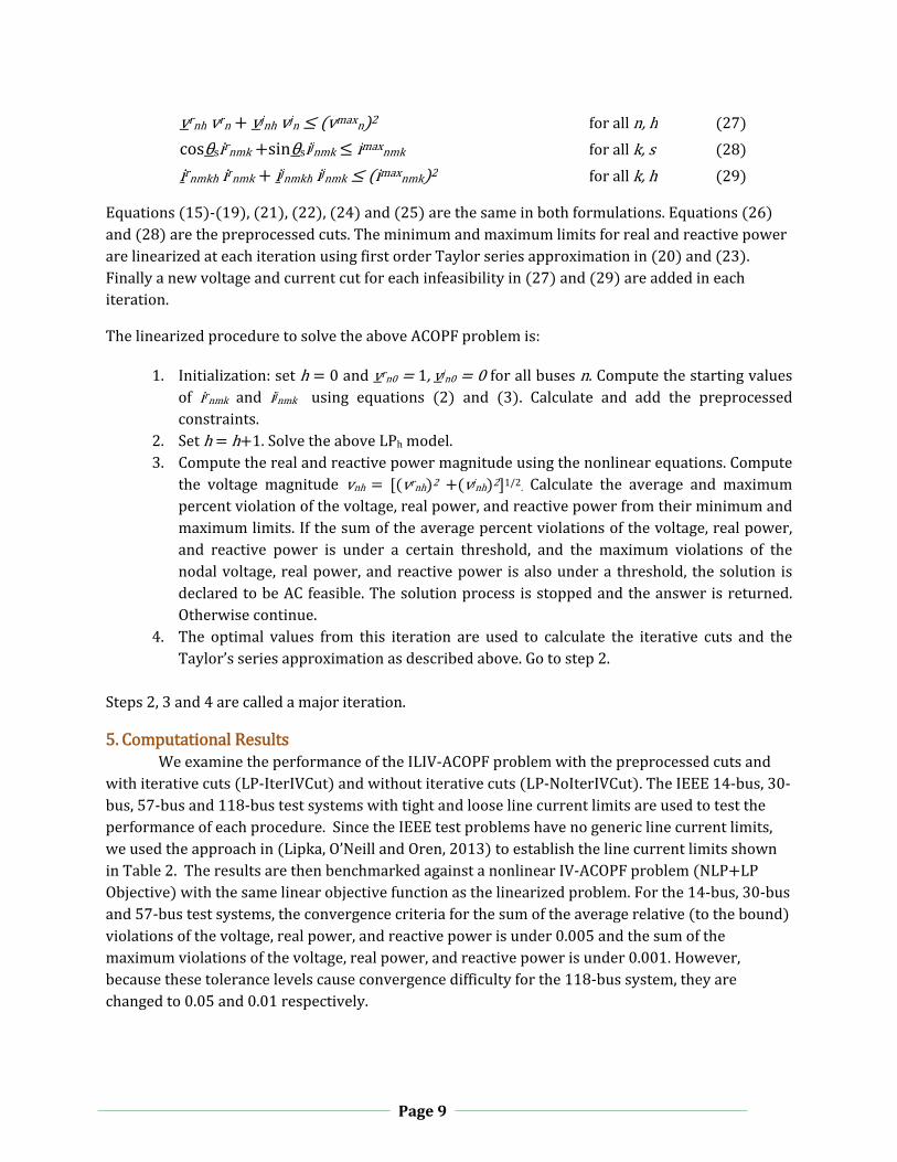
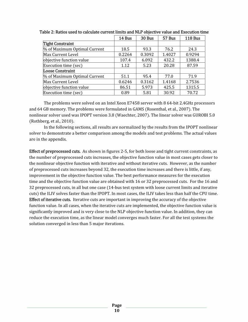
Inthefollowingsections,allresultsarenormalizedbytheresultsfromtheIPOPTnonlinearsolvertodemonstrateabettercomparisonamongthemodelsandtestproblems.Theactualvaluesareintheappendix.Effectofpreprocessedcuts.Asshowninfigures2‐5,forbothlooseandtightcurrentconstraints,asthenumberofpreprocessedcutsincreases,theobjectivefunctionvalueinmostcasesgetsclosertothenonlinearobjectivefunctionwithiterativeandwithoutiterativecuts.However,asthenumberofpreprocessedcutsincreasesbeyond32,theexecutiontimeincreasesandthereislittle,ifany,improvementintheobjectivefunctionvalue.Thebestperformancemeasuresfortheexecutiontimeandtheobjectivefunctionvalueareobtainedwith16or32preprocessedcuts.Forthe16and32preprocessedcuts,inallbutonecase 14‐bustestsystemwithloosecurrentlimitsanditerativecuts theILIVsolvesfasterthantheIPOPT.Inmostcases,theILIVtakeslessthanhalftheCPUtime.Effectofiterativecuts.Iterativecutsareimportantinimprovingtheaccuracyoftheobjectivefunctionvalue.Inallcases,whentheiterativecutsareimplemented,theobjectivefunctionvalueissignificantlyimprovedandisveryclosetotheNLPobjectivefunctionvalue.Inaddition,theycanreducetheexecutiontime,asthelinearmodelconvergesmuchfaster.Forallthetestsystemsthesolutionconvergedinlessthan5majoriterations.
Page 11
Page11
Figure2.ObjectiveFunctionPercentDifferenceandCPUTimeRelativetotheNonlinearSolverforLooseCurrentLimitandNoIterativeCuts
Figure3.ObjectiveFunctionPercentDifferenceandExecutionTimeRelativetotheNonlinearSolverforLooseCurrentLimitandIterativeCuts
Figure4.ObjectiveFunctionPercentDifferenceandExecutionTimeRelativetotheNonlinearSolverforTightCurrentLimitandNoIterativeCuts
0
0.2
0.4
0.6
0.8
1
1.2
1.4
4 16 32 128 360
Per
cen
t d
iffe
ren
ce
Number of Cuts
14-bus30-bus57-bus118-bus
Page 12
Page12
Figure5.ObjectiveFunctionPercentDifferenceandExecutionTimeRelativetotheNonlinearSolverforTightCurrentLimitandIterativeCuts6.ConclusionAsthenumberofpreprocessedconstraintsforeachbusandlineincreases,therelativeerrordecreases.Fortheproblemstested,theresultsindicatethat16to32constraintsarethebestnumberofpreprocessedconstraintsinatradeoffbetweenaccuracyandsolutiontime.Themarginalvalueofmorethan32andmaybe16preprocessedconstraintsinthissettingisnegative.Nevertheless,thenumberofpreprocessedconstraintscanbesetbasedontheperformanceandrequirementsofthespecificproblembeingsolved.Usingiterativecutsoftenresultsinfasterconvergencetoafeasiblesolution.Whensolvingwithoutusingiterativecuts,thesolutioniswithin18%ofthebest‐knownnonlinearfeasiblesolution;withiterativecuts,thesolutioniswithin2.5%ofthebest‐knownnonlinearsolution.At16or32preprocessedconstraints,solutiontimeisuptoabout8timesfasterthanthenonlinearsolver IPOPT .Thisapproachmaybeusefulinsolvingoptimaltransmissiontopologyandunitcommitmentproblemsbecausemixed‐integerlinearsolversaremuchfasterthanmixed‐linearnonlinearsolvers.
Page 13
Page13
ReferencesMaryB.Cain,RichardP.O’Neill,AnyaCastillo,“HistoryofOptimalPowerFlowandFormulations,”FERCStaffTechnicalPaper,December2012,http://www.ferc.gov/industries/electric/indus‐act/market‐planning/opf‐papers/acopf‐1‐history‐formulation‐testing.pdfFlorinCapitanescu,JoseLuisMartinezRamos,PatrickPanciatici,DanielKirschen,AlejandroMaranoMarcolini,LudovicPlatbrood,LouisWehenkel,“State‐of‐the‐art,challenges,andfuturetrendsinsecurityconstrainedoptimalpowerflow,”ElectricPowerSystemsResearch,August2011.J.Carpentier,"Contributionál’étudedudispatchingéconomique,"BulletindelaSociétéFrançaisedesÉlectriciens,vol.3,no.8,pp.431‐447,1962.AnyaCastilloandRichardPO’Neill,“SurveyofApproachestoSolvingtheACOPF”,FERCStaffTechnicalPaper,March2013a,http://www.ferc.gov/industries/electric/indus‐act/market‐planning/opf‐papers/acopf‐4‐solution‐techniques‐survey.pdf
AnyaCastilloandRichardPO’Neill,“ComputationalPerformanceofSolutionTechniquesAppliedtotheACOPF”,FERCStaffTechnicalPaper,March2013b,http://www.ferc.gov/industries/electric/indus‐act/market‐planning/opf‐papers/acopf‐5‐computational‐testing.pdf
H.W.DommelandW.F.Tinney,"OptimalPowerFlowSolutions,",IEEETransactionsonPowerApparatusandSystems,vol.PAS‐87,no.10,pp.1866‐1876,Oct.1968.FrankandI.Steponavice,"OptimalPowerFlow:aBibligraphicSurveyIFormulationsandDeterministicMethods,"EnergySyst,vol.3,pp.221‐258,2012.M.HuneaultandF.D.Galiana,,"Asurveyoftheoptimalpowerflowliterature,",IEEETransactionsonPowerSystems,vol.6,no.2,pp.762‐770,May1991PaulaA.Lipka,RichardP.O’Neill,andShmuelOren,“DevelopingLineCurrentmagnitudeConstraintsforIEEETestProblems”,FERCStaffTechnicalPaper,April2013.http://www.ferc.gov/industries/electric/indus‐act/market‐planning/opf‐papers/acopf‐7‐line‐constraints.pdf
J.A.Momoh,M.E.El‐Hawary,andR.Adapa,“AReviewofSelectedOptimalPowerFlowLiteratureto1993.PartI:NonlinearandQuadraticProgrammingApproaches”,IEEETrans.onPowerSystems,Vol.14 1 :pp.96‐104,Feb.1999.
RichardPO’Neill,AnyaCastilloandMaryCain,“TheIVFormulationandLinearApproximationsoftheACOptimalPowerFlowProblem,”FERCStaffTechnicalPaper,December2012a,http://www.ferc.gov/industries/electric/indus‐act/market‐planning/opf‐papers/acopf‐2‐iv‐linearization.pdf
Page 14
Page14
RichardPO’Neill,AnyaCastilloandMaryCain,“TheComputationalTestingofACOptimalPowerFlowUsingtheCurrentVoltageFormulations,”FERCStaffTechnicalPaper,December2012b,http://www.ferc.gov/industries/electric/indus‐act/market‐planning/opf‐papers/acopf‐3‐iv‐linearization‐testing.pdf
T.PotluriandK.W.Hedman,"ImpactsoftopologycontrolontheACOPF,"IEEEPowerandEnergySocietyGeneralMeeting,pp.1‐7,2012.R.E.RosenthalandA.Brooke,"GAMS,auser'sguide,"GAMSDevelopmentCorporation,2007.E.RothbergandR.Bixby,"Gurobioptimization,"2010.AaronSchecterandRichardPO’Neill,“ExplorationoftheACOPFFeasibleRegionfortheStandardIEEETestSet”,FERCStaffTechnicalPaper,February2013,http://www.ferc.gov/industries/electric/indus‐act/market‐planning/opf‐papers/acopf‐6‐test‐problem‐properties.pdf
B.Stott,O.AlsacandA.Monticelli,"DCpowerflowrevisited,"IEEETrans.PowerSyst.,vol.24,no.3,pp.1290‐1300,2009.BrianStottandOngunAlsaç,‘BasicRequirementsforReal‐LifeProblemsandTheirSolutions”,July1,2012,www.ieee.hr/_download/repository/Stott‐Alsac‐OPF‐White‐Paper.pdfWaechter,IntroductiontoIPOPT,CarnegieMellonUniversity,2007.
Page 15
Page15
APPENDIX:NUMERICALRESULTS
14‐BUSSYSTEMTableA1:ObjectiveFunctionValues:14‐bussystem,tightcurrentconstraint
Number ofcuts 4 16 32 128 360
LP‐NoIterIVCut 89.2100 99.9100 105.3400 106.6800 107.0600LP‐IterIVCut 106.5500 105.6900 106.5300 106.9400 107.0700NLP LPObj 107.3686 107.3686 107.3686 107.3686 107.3686
TableA2:ExecutionTime:14‐bussystem,tightcurrentconstraint
Number ofcuts4 16 32 128 360
LP‐NoIterIVCut 1.940 0.220 1.070 1.170 2.660LP‐IterIVCut 0.140 0.300 0.310 1.280 2.580NLP LPObj 1.125 1.125 1.125 1.125 1.125
TableA3:ObjectiveFunctionValues:14‐bussystem,loosecurrentconstraint
Number ofcuts 4 16 32 128 360
LP‐NoIterIVCut 79.7700 85.8100 86.0500 86.1600 86.1700LP‐IterIVCut 86.0900 85.9600 85.9600 86.1600 86.1700NLP LPObj 86.5062 86.5062 86.5062 86.5062 86.5062
TableA4:ExecutionTime:14‐bussystem,loosecurrentconstraint
Number ofcuts 4 16 32 128 360
LP‐NoIterIVCut 1.690 0.170 0.230 0.830 2.420LP‐IterIVCut 0.190 0.790 1.030 1.490 4.760NLP LPObj 0.891 0.891 0.891 0.891 0.891
30‐BUSSYSTEMTableA5:ObjectiveFunctionValues:30‐bussystem,tightcurrentlimit
Numberofcuts 4 16 32 128 360LP‐NoIterIVCut 5.8200 5.9600 6.0300 6.0900 6.1000LP‐IterIVCut 6.0100 6.0600 6.0800 6.0900 6.1000NLP LPObj 6.0920 6.0920 6.0920 6.0920 6.0920
TableA6:ExecutionTime:30‐bussystem,tightcurrentlimit
Numberofcuts 4 16 32 128 360LP‐NoIterIVCut 4.540 0.950 0.990 3.870 10.520LP‐IterIVCut 0.270 0.630 1.310 4.010 10.090NLP LPObj 5.234 5.234 5.234 5.234 5.234
Page 16
Page16
TableA7:ObjectiveFunctionValues:30‐bussystem,loosecurrentlimitNumberofcuts 4 16 32 128 360LP‐NoIterIVCut 5.8200 5.9300 5.9700 5.9700 5.9700LP‐IterIVCut 5.9500 5.9800 5.9800 5.9700 5.9700NLP LPObj 5.9738 5.9738 5.9738 5.9738 5.9738
Table3:executionTime:30‐bussystem,loosecurrentlimit
Numberofcuts 4 16 32 128 360LP‐NoIterIVCut 16.870 1.490 1.420 3.310 10.600LP‐IterIVCut 0.480 1.630 2.400 5.340 15.330NLP LPObj 5.812 5.812 5.812 5.812 5.812
57‐BUSSYSTEMTableA9:ObjectiveFunctionValues:57‐bussystem,tightcurrentlimit
Numberofcuts 4 16 32 128 360LP‐NoIterIVCut 416.9117 422.9959 422.8063 422.4807 422.5419LP‐IterIVCut 422.6372 423.4306 422.7098 422.4812 422.5419NLP LPObj 432.1900 432.1900 432.1900 432.1900 432.1900
TableA10:executionTime:57‐bussystem,tightcurrentlimit
Numberofcuts 4 16 32 128 360LP‐NoIterIVCut 19.709 2.436 5.780 27.088 87.331LP‐IterIVCut 1.127 2.041 4.832 21.268 59.018NLP LPObj 20.281 20.281 20.281 20.281 20.281
TableA11:ObjectiveFunctionValues:57‐bussystem,loosecurrentlimit
Numberofcuts 4 16 32 128 360LP‐NoIterIVCut 416.7944 424.7595 422.4737 422.3770 422.4237LP‐IterIVCut 422.0834 422.5992 422.4155 422.3798 422.4236NLP LPObj 425.4805 425.4805 425.4805 425.4805 425.4805
TableA12:ExecutionTime:57‐bussystem,loosecurrentlimitNumberofcuts 4 16 32 128 360LP‐NoIterIVCut 16.144 1.969 4.545 21.344 76.306LP‐IterIVCut 0.989 2.874 6.614 24.608 60.344NLP LPObj 30.922 30.922 30.922 30.922 30.922
Page 17
Page17
118‐BUSSYSTEMTableA13:ObjectiveFunctionValues:118‐bussystem,tightcurrentlimit
Numberofcuts 4 16 32 128 360LP‐ 1357.1281 1383.0689 1379.9237 1379.1194 1379.0062
LP‐IterIVCut 1382.1567 1381.0145 1380.2231 1379.1220 1379.0067NLP LPObj 1388.4251 1388.4251 1388.4251 1388.4251 1388.4251
TableA14:ExecutionTime:118‐bussystem,tightcurrentlimit
Numberofcuts 4 16 32 128 360LP‐NoIterIVCut 93.134 14.373 18.289 73.726 124.514LP‐IterIVCut 38.001 8.472 15.817 53.749 124.637NLP LPObj 87.594 87.594 87.594 87.594 87.594
Table4:ObjectiveFunctionValues:118‐bussystem,loosecurrentlimit
Numberofcuts 4 16 32 128 360LP‐ 1268.3334 1284.7513 1295.2132 1295.8839 1291.0350
LP‐IterIVCut 1287.1712 1287.5420 1298.0719 1291.0000 1296.2755NLP LPObj 1315.4988 1315.4988 1315.4988 1315.4988 1315.4988
Table5:ExecutionTime:118‐bussystem,loosecurrentlimit
Numberofcuts 4 16 32 128 360LP‐NoIterIVCut 68.232 259.395 446.980 1885.862 3869.237LP‐IterIVCut 130.440 256.572 438.003 1497.221 3983.677NLP LPObj 70.719 70.719 70.719 70.719 70.719