http://www.econometricsociety.org/ Econometrica, Vol. 82, No. 2 (March, 2014), 765–784 OPTIMAL TEST FOR MARKOV SWITCHING PARAMETERS MARINE CARRASCO University of Montreal, Montréal, Quebec H3C3J7, Canada LIANG HU Wayne State University, Detroit, MI 48202, U.S.A. WERNER PLOBERGER Washington University in St. Louis, St. Louis, MO 63130, U.S.A. The copyright to this Article is held by the Econometric Society. It may be downloaded, printed and reproduced only for educational or research purposes, including use in course packs. No downloading or copying may be done for any commercial purpose without the explicit permission of the Econometric Society. For such commercial purposes contact the Office of the Econometric Society (contact information may be found at the website http://www.econometricsociety.org or in the back cover of Econometrica). This statement must be included on all copies of this Article that are made available electronically or in any other format.
MARINE CARRASCOUniversity of Montreal, Montréal, Quebec H3C3J7, Canada
LIANG HUWayne State University, Detroit, MI 48202, U.S.A.
WERNER PLOBERGERWashington University in St. Louis, St. Louis, MO 63130, U.S.A.
The copyright to this Article is held by the Econometric Society. It may be downloaded,printed and reproduced only for educational or research purposes, including use in coursepacks. No downloading or copying may be done for any commercial purpose without theexplicit permission of the Econometric Society. For such commercial purposes contactthe Office of the Econometric Society (contact information may be found at the websitehttp://www.econometricsociety.org or in the back cover of Econometrica). This statement mustbe included on all copies of this Article that are made available electronically or in any otherformat.
BY MARINE CARRASCO, LIANG HU, AND WERNER PLOBERGER1
This paper proposes a class of optimal tests for the constancy of parameters in ran-dom coefficients models. Our testing procedure covers the class of Hamilton’s models,where the parameters vary according to an unobservable Markov chain, but also appliesto nonlinear models where the random coefficients need not be Markov. We show thatthe contiguous alternatives converge to the null hypothesis at a rate that is slower thanthe standard rate. Therefore, standard approaches do not apply. We use Bartlett-typeidentities for the construction of the test statistics. This has several desirable properties.First, it only requires estimating the model under the null hypothesis where the param-eters are constant. Second, the proposed test is asymptotically optimal in the sense thatit maximizes a weighted power function. We derive the asymptotic distribution of ourtest under the null and local alternatives. Asymptotically valid bootstrap critical valuesare also proposed.
KEYWORDS: Information matrix test, optimal test, Markov switching model, Ney-man–Pearson lemma, random coefficients model.
1. INTRODUCTION
IN THIS PAPER, WE FOCUS ON testing the constancy of parameters in dynamicmodels. The parameters are constant under the null hypothesis, whereas theyare random and weakly dependent under the alternative. The model of inter-est is very general and includes as a special case the state space models andthe Markov switching model initially introduced by Baum and Petrie (1966)and further studied by Hamilton (1989), where the regime changes in the pa-rameters are driven by an unobservable two-state Markov chain. The modelunder the null need not be linear and could be a GARCH model, for instance.Moreover, the random coefficients need not be Markov.
Two distinct features make testing the stability of coefficients particularlychallenging. The first is that the hyperparameters that enter in the dynamicsof the random coefficients are not identified under the null hypothesis. As aresult, the usual tests, like the likelihood ratio test, do not have a chi-squareddistribution. The second feature is that the information matrix is singular un-der the null hypothesis. This is due to the fact that the underlying regimesare not observable. The first feature, known as the problem of nuisance pa-rameters that are not identified under the null hypothesis, also arises whentesting for structural change or threshold effects. It has been investigated inmany papers, for example, Davies (1977, 1987), Andrews (1993), Andrews and
1An earlier version of this paper has circulated under the title “Optimal Test for MarkovSwitching.” The authors are grateful to an editor and three referees for helpful comments. Car-rasco gratefully acknowledges partial financial support from the National Science Foundationunder Grant SES-0211418.
Ploberger (1994), Hansen (1996), among others. However, the second featureof our testing problem implies that the “right” (i.e., contiguous) local alterna-tives are of order T−1/4 (where T is the sample size), while they are of the orderT−1/2 in the case of structural change and threshold models. The asymptotic lo-cal optimality discussed below shows that there do not exist tests with nontrivialpower against local alternatives that converge faster than T−1/4. Therefore, itis necessary to consider this rate of convergence when discussing power. Con-sequently, the results of Andrews and Ploberger (1994) do not apply here andwe need to expand the likelihood to the fourth order to derive the propertiesof our test.
Our contribution is twofold. First, we propose a new test for parameter sta-bility. This test is based on functionals of the first two derivatives of the like-lihood evaluated under the null and the autocorrelations of the process de-scribing the random parameters. It can be viewed as a time-series extension ofWhite’s (1982) information matrix test and shares some of its advantages. Inparticular, it requires the estimation of the model under the null hypothesisonly. This feature is particularly desirable when bootstrapping critical values.Another advantage of our test is that it does not require a full specification ofthe dynamics of the random coefficients. We only need to know their covari-ance structure. It means that our test will have power against a wide variety ofalternatives. The second contribution of our paper is to show that the proposedtest is asymptotically locally optimal in the sense that there exists no test that ismore powerful for a specific alternative that we are going to characterize. Theproof consists in showing that, for fixed values of the nuisance parameters, ourtest is asymptotically locally equivalent to the likelihood ratio test. Then, thenuisance parameters are integrated out with respect to some prior distribution.We appeal to the Neyman–Pearson lemma to prove optimality.
There are few papers proposing tests for Markov switching. Garcia (1998)studied the asymptotic distribution of a sup-type likelihood ratio test. Hansen(1992) treated the likelihood as an empirical process indexed by all the param-eters (those identified and those unidentified under the null). His test reliedon taking the supremum of LR over the nuisance parameters. Both papersrequire estimating the model under the alternatives, which may be cumber-some. None investigates local powers. Gong and Mariano (1997) reparameter-ized their linear model in the frequency domain and constructed a test basedon the differences in the spectrum between null and alternative. A Bayesianmodel selection procedure for Markov switching was proposed by Kim andNelson (2001).
The connection between the information matrix test of White (1982) andthe score test for independent mixture has been outlined by Chesher (1984).Lee and Chesher (1986) showed that, when the information matrix is singular,the likelihood ratio test may only have power against local alternatives of or-der T−1/4 but remains optimal provided the true parameter vector under H0
is an interior point of the parameter space. Recently, Cho and White (2007)proposed a likelihood ratio test for an independent and identically distributed
OPTIMAL TEST FOR MARKOV SWITCHING PARAMETERS 767
(i.i.d.) mixture in dynamic models and showed that this test has power againstMarkov switching alternatives even though it ignores the temporal dependenceof the Markov chain.
Published applications of our test include Hamilton (2005), Warne andVredin (2006), Kahn and Rich (2007), Hu and Shin (2008), Morley and Piger(2012), and Dufrénot, Mignon, and Péguin-Feissolle (2011).
The outline of the paper is as follows. Section 2 describes the test statistic.Section 3 derives the null distribution of the test and a bootstrap method tocompute its p-values. Section 4 establishes the optimality. Section 5 investi-gates the power of the test. In Section 6, we describe simulation results andinvestigate the nonlinearity in the GNP growth. Using U.S. data over the past60 years, we found that while our test cannot reject the null hypothesis of a lin-ear model against a Markov switching mean, it strongly rejects the same nullagainst varying mean and variance. Finally, Section 7 concludes. Further ex-amples and the proofs are collected in the Supplemental Material (Carrasco,Hu, and Ploberger (2014); CHP hereafter). Moreover, Appendix B of CHPdefines the tensor notations used to derive the fourth order expansion of thelikelihood. These notations are interesting in their own right, as they could beused in other econometric problems involving higher-order expansions.
2. ASSUMPTIONS AND TEST STATISTIC
The observations are denoted by y1� y2� � � � � yT (univariate or multivariate).Let ft(·) denote the conditional density (with respect to some dominating mea-sure) of yt given yt−1� � � � � y1. ft(·) is known up to a p-dimensional vector ofparameters, say θt . We are interested in testing whether these parameters areconstant over time. Namely, we test
H0 :θt = θ0� for some unspecified θ0(2.1)
against
H1 :θt = θ0 +ηt�(2.2)
where the switching variable ηt is not observable. We will construct asymp-totically optimal tests for this testing problem under some assumptions onthe structure of the ηt . So our basic probability spaces are the sets of all(y1� y2� � � � � yT �η1�η2� � � � �ηT ).
ASSUMPTION 1: The latent variable ηt is stationary and its distribution maydepend on some unknown parameters β. They are nuisance parameters thatare not identified under H0. We assume that β belongs to a compact set B.Moreover, ηt is strongly exogenous in the sense that the joint likelihood of(y1� y2� � � � � yT �η1�η2� � � � �ηT ) factorizes as
∏T
t=1 f (yt |θt� yt−1� yt−2� � � � � y1)q(ηt |ηt−1�ηt−2� � � � �η1;β) and the values of θt belong to some compact subset of R
p,Θ, containing θ0.
768 M. CARRASCO, L. HU, AND W. PLOBERGER
So we assume that even under the null there exists a distribution of the ηt .Nevertheless, under the null (2.1), this distribution does not play any role withregard to the distribution of the data (yT � yT−1� yT−2� � � � � y1). Under H0, theyt and the ηt are mutually independent. Hence we can—when we fix θ0—consider our null to be simple.
ASSUMPTION 2: yt is stationary under H0 and the following conditions on theconditional log-density of yt given yt−1� � � � � y1 (under H0), lt , are satisfied: lt =lt(θ), as a function of the parameter θ, is at least five times differentiable, and fork= 1� � � � �5,
Eθ0 supθ∈N
(∥∥l(k)t (θ)∥∥20)
<∞�
where l(k)t denotes the kth derivative of the log-likelihood with respect to the pa-rameter θ and N is a neighborhood around θ0. Eθ0 is the expectation with respectto the probability measure corresponding to the parameter θ0 and ‖ · ‖ denotes theFrobenius norm. Moreover, θ0 is an interior point of Θ and the information matrixI(θ0)=Eθ0(l
(1)t (θ0)l
(1)′t (θ0)) is nonsingular.
REMARK 1: Assumption 2 is maintained for mathematical convenience. Itguarantees, in particular, the uniform convergence of the information matrixand the consistency and asymptotic normality of the maximum likelihood es-timator (MLE) of θ under H0. Suitable generalizations of the Kolmogorov–Cencov theorem (cf. Kunita (1990, Theorem 1.4.7, p. 38)) might yield criteriawhich only depend on expressions like supθ∈N Eθ0(‖l(k)t (θ)‖M). However, wethink that the present version is general enough to cover most of the standardcases. In Section A.2 of CHP, we show that Assumption 2 is satisfied for ARCHand GARCH models with normal errors.
REMARK 2: As in Andrews and Ploberger (1994, Section 4.1), the vector ofobservable variables yt may include exogenous variables. We do not impose re-strictions on the moments of yt . For instance, yt could be a stationary IGARCHprocess. However, we rule out the case where yt is a random walk. To deal withunit root, we would have to alter the test statistic by proper rescaling, and itsasymptotic distribution would be different; see Hu (2011).
For technical reasons, we need to maintain some restrictions on the pro-cess ηt .
ASSUMPTION 3: ηt is a function κ of a latent Markov process ϑt . We assumethat ϑt is stationary and β-mixing with geometric decay. It implies in particularthat there exist 0 < λ< 1 and a measurable nonnegative function g such that
sup|h|≤1
∣∣E[h(ϑt+m)|ϑt
] −E[h(ϑt)
]∣∣ ≤ λmg(ϑt)�(2.3)
OPTIMAL TEST FOR MARKOV SWITCHING PARAMETERS 769
and Eg(ϑt) < ∞. Furthermore, we assume that Eηt = 0 and maxt ‖ηt‖ ≤M < ∞. Moreover, the constant λ and the bound M are independent of β de-fined in Assumption 1 and E‖g‖ can be bounded by a constant independent of β.Finally, E(ηtηt−k), for any integer k, is assumed to be continuous in β.
The assumption Eηt = 0 is not restrictive, as the model can always be repa-rameterized to ensure this condition. ϑt β-mixing is satisfied by, for example,an irreducible and aperiodic Markov chain with finite state space. The prop-erty that ϑt is β-mixing with geometric decay will imply that ηt is geomet-ric ergodic. maxt ‖ηt‖ ≤ M < ∞ will also be satisfied by any finite state spaceMarkov chain; however, it will not be satisfied by an AR(1) process with nor-mal error. This condition could be relaxed to allow for distributions of ηt withthin tails, but this extension is beyond the scope of the present paper. Althoughsome form of mixing is necessary for the ηt , one should be able to relax condi-tion (2.3).
Note that Assumption 3 does not require ηt itself to be Markov. Our as-sumption allows, for example, ηt to be a MA-process of the form
ηt = et + a1et−1 + · · · + apet−p�
where the et are i.i.d. In this case, ϑt = (ηt� et� � � � � et−p)′ is Markov. This ex-
ample illustrates the potential autocorrelation functions of ηt . In fact, the setof autocorrelations satisfying our assumption approximates an arbitrary auto-correlation in any of the usual topologies.
The test statistic TST , for a given β, is of the form
TST (β) = TST (β� θ̂) = ΓT − 12T
ε̂(β)′ε̂(β)�(2.4)
where ΓT = 1√T
∑t μ2�t(β� θ̂) with
μ2�t(β�θ) = 12
(tr
((l(2)t + l(1)t l(1)′t
)Eβ
(ηtη
′t
))(2.5)
+ 2∑s<t
tr(l(1)t l(1)′s Eβ
(ηtη
′s
)))�
where tr denotes the trace and ε̂(β) is the residual from the OLS regression ofμ2�t(β� θ̂) on l(1)t (θ̂), and θ̂ is the constrained maximum likelihood estimator ofθ under H0 (i.e., the ML estimator under the assumption of constant parame-ters). As β is unknown and cannot be estimated consistently under H0, we usesup-type tests as in Davies (1987):
supTS = supβ∈B̄
TST (β)�
770 M. CARRASCO, L. HU, AND W. PLOBERGER
or exponential-type tests as in Andrews and Ploberger (1994):
expTS =∫B̄
exp(TST (β)
)dJ(β)�(2.6)
where J is some prior distribution for β with support on B̄, a compact subsetof B. We will establish admissibility for a class of expTS statistics.
REMARKS: 1. In some applications, it may be of interest to test for the vari-ability of one subset of parameters. To accommodate this case, it suffices toset the elements of ηt corresponding to the constant coefficients equal to zero.Then, ΓT involves only the elements of the score and Hessian correspondingto the varying coefficients. However, in the computation of ε̂(β), one needs toproject μ2�t(β� θ̂) on the whole vector l(1)t (θ̂) (including the score with respectto the constant coefficients).
2. The test statistic TST (β) depends only on the score and derivative of thescore under the null and on the estimator of θ under H0. Therefore, it does notrequire estimating the model under the alternative. This is a great advantagewhen applying bootstrap to compute the critical values or p-values of the test.
3. The test relies on the second Bartlett identity (Bartlett (1953a, 1953b))and is related to the information matrix test introduced by White (1982). Later,Chesher (1984) showed that the score test of the hypothesis that random coef-ficients have zero variance is equivalent to the information matrix test. David-son and MacKinnon (1991) derived information-matrix-type tests for testingrandom parameters. Both papers assumed that the random parameters are in-dependent, whereas we assume that the parameters are serially correlated andwe fully exploit this correlation. As shown in Equation (2.5), our test statisticsinvolve the second derivatives of the log-likelihood and the outer products ofthe scores as in the information matrix test, plus an extra term. This term actu-ally arises from the serial dependence of the time-varying coefficients. Specif-ically, it captures the correlations between the conditional scores at differenttime periods.
4. The form of our test depends on the latent process ηt solely through itssecond-order properties.
5. We assume throughout the paper that the model under the null is correctlyspecified. The issue of misspecification is not addressed here.
3. NULL DISTRIBUTION AND IMPLEMENTATION
First of all, we establish the distribution of the test statistics under the null.For this purpose, define
d(β)= d(β�θ0)= (I(θ0)
)−1cov
(μ2�t(β�θ0)� l
(1)t (θ0)
)�(3.1)
OPTIMAL TEST FOR MARKOV SWITCHING PARAMETERS 771
where I(θ0) denotes the information matrix of θ under H0. Then, we have thefollowing result.
THEOREM 3.1: Under H0,(i) ΓT converges to a Gaussian process, N(β), with mean 0 and covariance
∑ε̂2t (β) converges to Eθ0((μ2�t(β�θ0) − d(β)′l(1)t (θ0))
2) in probabilityuniformly in β.
(iii) TST (β) converges weakly to N(β)− 12k(β�β) and
supTSd→ sup
β∈B̄
{N(β)− 1
2k(β�β)
}�
expTSd→
∫B̄
exp(N(β)− 1
2k(β�β)
)dJ(β)�
The asymptotic distribution of the test statistic might not be nuisance param-eter free. We think that the advantage of being optimal outweighs this disad-vantage. Modern computing technology makes it possible to get critical valuesby parametric bootstrapping (see Davidson and MacKinnon (2004) or Hall(1992)). In particular, we propose the following strategy to approximate the αcritical values cα and the p-value of expTS (the same strategy can be used forsupTS):
1. Using the observed data, estimate θ0 by θ̂, the maximum likelihood esti-mator under H0. Compute the test statistic expTS.
2. Given θ̂, generate S independent samples {ys1� � � � � y
sT }s=1�����S under H0
with θ = θ̂.3. Using each simulated sample {ys
1� � � � � ysT }, estimate θ by θ̂s the MLE un-
der H0 and compute expTS with θ̂s. The resulting statistics are denoted expTSs,s = 1�2� � � � � S.
4. Define cα�S as the empirical critical values using expTSs, s = 1�2� � � � � S,that is, cα�S is the (1 − α) quantile of expTSs, s = 1�2� � � � � S. Moreover, thebootstrap p-value is given by 1
S
∑S
s=1 I(expTSs > expTS).Letting S → ∞ will force the empirical critical values to converge to the
critical values for the distribution of the test statistic under Pθ̂. We will provethat when T goes to infinity, these critical values converge to the true ones (theones corresponding to the data generated by a Pθ0 , θ0 ∈ H0). It should be notedthat the consistency of the above bootstrap is also preserved under contiguouslocal alternatives. Contiguity guarantees that convergence under the null alsoholds true under the probability measure describing the local alternative.
THEOREM 3.2: The bootstrap critical values cα�S converge to cα in probabilityas T and S go to infinity under H0 and under local alternatives θT = θ0 + h/
√T .
772 M. CARRASCO, L. HU, AND W. PLOBERGER
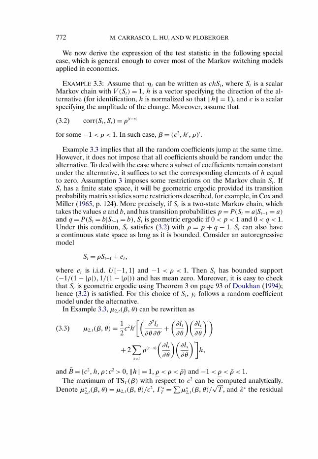
We now derive the expression of the test statistic in the following specialcase, which is general enough to cover most of the Markov switching modelsapplied in economics.
EXAMPLE 3.3: Assume that ηt can be written as chSt , where St is a scalarMarkov chain with V (St) = 1, h is a vector specifying the direction of the al-ternative (for identification, h is normalized so that ‖h‖ = 1), and c is a scalarspecifying the amplitude of the change. Moreover, assume that
corr(St� Ss)= ρ|t−s|(3.2)
for some −1 < ρ< 1. In such case, β= (c2�h′�ρ)′.
Example 3.3 implies that all the random coefficients jump at the same time.However, it does not impose that all coefficients should be random under thealternative. To deal with the case where a subset of coefficients remain constantunder the alternative, it suffices to set the corresponding elements of h equalto zero. Assumption 3 imposes some restrictions on the Markov chain St . IfSt has a finite state space, it will be geometric ergodic provided its transitionprobability matrix satisfies some restrictions described, for example, in Cox andMiller (1965, p. 124). More precisely, if St is a two-state Markov chain, whichtakes the values a and b, and has transition probabilities p = P(St = a|St−1 = a)and q = P(St = b|St−1 = b), St is geometric ergodic if 0 <p< 1 and 0 < q < 1.Under this condition, St satisfies (3.2) with ρ = p + q − 1. St can also havea continuous state space as long as it is bounded. Consider an autoregressivemodel
St = ρSt−1 + et�
where et is i.i.d. U[−1�1] and −1 < ρ < 1. Then St has bounded support(−1/(1 − |ρ|)�1/(1 − |ρ|)) and has mean zero. Moreover, it is easy to checkthat St is geometric ergodic using Theorem 3 on page 93 of Doukhan (1994);hence (3.2) is satisfied. For this choice of St , yt follows a random coefficientmodel under the alternative.
In Example 3.3, μ2�t(β�θ) can be rewritten as
μ2�t(β�θ) = 12c2h′
[(∂2lt
∂θ∂θ′ +(∂lt
∂θ
)(∂lt
∂θ
)′)(3.3)
+ 2∑s<t
ρ(t−s)
(∂lt
∂θ
)(∂ls
∂θ
)′]h�
and B̄ = {c2�h�ρ : c2 > 0�‖h‖ = 1�ρ < ρ < ρ̄} and −1 < ρ< ρ̄ < 1.The maximum of TST (β) with respect to c2 can be computed analytically.
Denote μ∗2�t(β�θ) = μ2�t(β�θ)/c
2, Γ ∗T = ∑
μ∗2�t(β�θ)/
√T , and ε̂∗ the residual
OPTIMAL TEST FOR MARKOV SWITCHING PARAMETERS 773
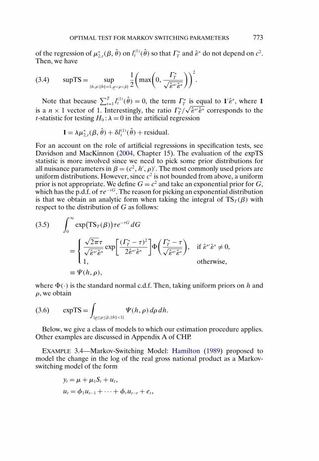
of the regression of μ∗2�t(β� θ̂) on l(1)t (θ̂) so that Γ ∗
T and ε̂∗ do not depend on c2.Then, we have
supTS = sup{h�ρ:‖h‖=1�ρ<ρ<ρ̄}
12
(max
(0�
Γ ∗T√
ε̂∗′ε̂∗
))2
�(3.4)
Note that because∑T
t=1 l(1)t (θ̂) = 0, the term Γ ∗
T is equal to 1′ε̂∗, where 1is a n × 1 vector of 1. Interestingly, the ratio Γ ∗
T /√ε̂∗′ε̂∗ corresponds to the
t-statistic for testing H0 :λ= 0 in the artificial regression
1 = λμ∗2�t(β� θ̂)+ δl(1)t (θ̂)+ residual�
For an account on the role of artificial regressions in specification tests, seeDavidson and MacKinnon (2004, Chapter 15). The evaluation of the expTSstatistic is more involved since we need to pick some prior distributions forall nuisance parameters in β = (c2�h′�ρ)′. The most commonly used priors areuniform distributions. However, since c2 is not bounded from above, a uniformprior is not appropriate. We define G= c2 and take an exponential prior for G,which has the p.d.f. of τe−τG. The reason for picking an exponential distributionis that we obtain an analytic form when taking the integral of TST (β) withrespect to the distribution of G as follows:∫ ∞
0exp
(TST (β)
)τe−τG dG(3.5)
=⎧⎨⎩
√2πτ√ε̂∗′ε̂∗
exp[(Γ ∗
T − τ)2
2ε̂∗′ε̂∗
]�
(Γ ∗T − τ√ε̂∗′ε̂∗
)� if ε̂∗′ε̂∗ = 0,
1� otherwise,
≡Ψ(h�ρ)�
where �(·) is the standard normal c.d.f. Then, taking uniform priors on h andρ, we obtain
expTS =∫
{ρ≤ρ≤ρ�‖h‖<1}Ψ(h�ρ)dρdh�(3.6)
Below, we give a class of models to which our estimation procedure applies.Other examples are discussed in Appendix A of CHP.
EXAMPLE 3.4—Markov-Switching Model: Hamilton (1989) proposed tomodel the change in the log of the real gross national product as a Markov-switching model of the form
yt = μ+μ1St + ut�
ut =φ1ut−1 + · · · +φrut−r + et�
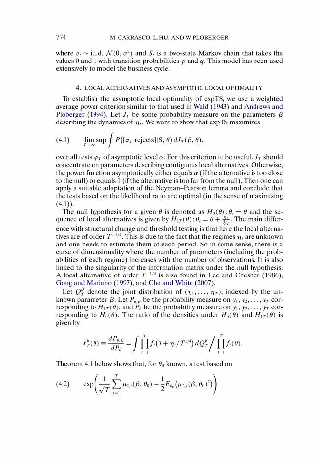
774 M. CARRASCO, L. HU, AND W. PLOBERGER
where et ∼ i�i�d� N (0�σ2) and St is a two-state Markov chain that takes thevalues 0 and 1 with transition probabilities p and q. This model has been usedextensively to model the business cycle.
4. LOCAL ALTERNATIVES AND ASYMPTOTIC LOCAL OPTIMALITY
To establish the asymptotic local optimality of expTS, we use a weightedaverage power criterion similar to that used in Wald (1943) and Andrews andPloberger (1994). Let JT be some probability measure on the parameters βdescribing the dynamics of ηt . We want to show that expTS maximizes
limT→∞
sup∫
P([ϕT rejects]|β�θ)
dJT (β�θ)�(4.1)
over all tests ϕT of asymptotic level α. For this criterion to be useful, JT shouldconcentrate on parameters describing contiguous local alternatives. Otherwise,the power function asymptotically either equals α (if the alternative is too closeto the null) or equals 1 (if the alternative is too far from the null). Then one canapply a suitable adaptation of the Neyman–Pearson lemma and conclude thatthe tests based on the likelihood ratio are optimal (in the sense of maximizing(4.1)).
The null hypothesis for a given θ is denoted as H0(θ) :θt = θ and the se-quence of local alternatives is given by H1T (θ) :θt = θ + ηt
4√T
. The main differ-ence with structural change and threshold testing is that here the local alterna-tives are of order T−1/4. This is due to the fact that the regimes ηt are unknownand one needs to estimate them at each period. So in some sense, there is acurse of dimensionality where the number of parameters (including the prob-abilities of each regime) increases with the number of observations. It is alsolinked to the singularity of the information matrix under the null hypothesis.A local alternative of order T−1/4 is also found in Lee and Chesher (1986),Gong and Mariano (1997), and Cho and White (2007).
Let QβT denote the joint distribution of (η1� � � � �ηT ), indexed by the un-
known parameter β. Let Pθ�β be the probability measure on y1� y2� � � � � yT cor-responding to H1T (θ), and Pθ be the probability measure on y1� y2� � � � � yT cor-responding to H0(θ). The ratio of the densities under H0(θ) and H1T (θ) isgiven by
�βT (θ) ≡ dPθ�β
dPθ
=∫ T∏
t=1
ft(θ+ηt/T
1/4)dQβ
T
/ T∏t=1
ft(θ)�
Theorem 4.1 below shows that, for θ0 known, a test based on
exp
(1√T
T∑t=1
μ2�t(β�θ0)− 12Eθ0
(μ2�t(β�θ0)
2))
(4.2)
OPTIMAL TEST FOR MARKOV SWITCHING PARAMETERS 775
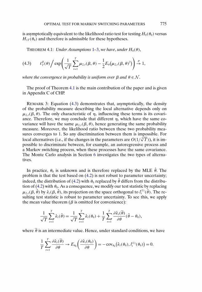
is asymptotically equivalent to the likelihood ratio test for testing H0(θ0) versusH1T (θ0) and therefore is admissible for these hypotheses.
THEOREM 4.1: Under Assumptions 1–3, we have, under H0(θ),
�βT (θ)/
exp
(1√T
T∑t=1
μ2�t(β�θ)− 12Eθ
(μ2�t(β�θ)
2)) P→ 1�(4.3)
where the convergence in probability is uniform over β and θ ∈ N .
The proof of Theorem 4.1 is the main contribution of the paper and is givenin Appendix C of CHP.
REMARK 3: Equation (4.3) demonstrates that, asymptotically, the densityof the probability measure describing the local alternative depends only onμ2�t(β�θ). The only characteristic of ηt influencing these terms is its covari-ance. Therefore, we may conclude that different ηt which have the same co-variance will have the same μ2�t(β�θ), hence generating the same probabilitymeasure. Moreover, the likelihood ratio between these two probability mea-sures converges to 1. So any discrimination between them is impossible. Forlocal alternatives (i.e., if the changes in the parameters are O(1/ 4
√T)), it is im-
possible to discriminate between, for example, an autoregressive process anda Markov switching process, when these processes have the same covariance.The Monte Carlo analysis in Section 6 investigates the two types of alterna-tives.
In practice, θ0 is unknown and is therefore replaced by the MLE θ̂. Theproblem is that the test based on (4.2) is not robust to parameter uncertainty;indeed, the distribution of (4.2) with θ0 replaced by θ̂ differs from the distribu-tion of (4.2) with θ0. As a consequence, we modify our test statistic by replacingμ2�t(β� θ̂) by ε̂t(β� θ̂), its projection on the space orthogonal to l(1)t (θ̂). The re-sulting test statistic is robust to parameter uncertainty. To see this, we applythe mean value theorem (β is omitted for convenience):
1√T
T∑t=1
ε̂t(θ̂) = 1√T
T∑t=1
ε̂t(θ0)+ 1T
T∑t=1
∂ε̂t(θ)
∂θ(θ̂− θ0)�
where θ is an intermediate value. Hence, under standard conditions, we have
1T
T∑t=1
∂ε̂t(θ)
∂θ→Eθ0
(∂ε̂t(θ0)
∂θ
)= − covθ0
(ε̂t(θ0)� l
(1)t (θ0)
) = 0�
776 M. CARRASCO, L. HU, AND W. PLOBERGER
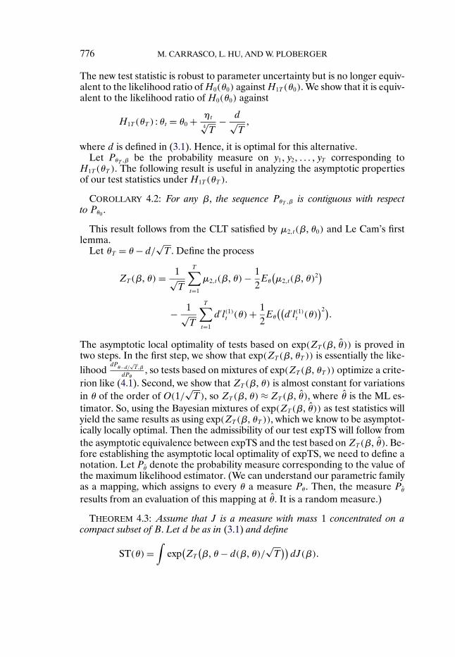
The new test statistic is robust to parameter uncertainty but is no longer equiv-alent to the likelihood ratio of H0(θ0) against H1T (θ0). We show that it is equiv-alent to the likelihood ratio of H0(θ0) against
H1T (θT ) :θt = θ0 + ηt
4√T
− d√T�
where d is defined in (3.1). Hence, it is optimal for this alternative.Let PθT �β be the probability measure on y1� y2� � � � � yT corresponding to
H1T (θT ). The following result is useful in analyzing the asymptotic propertiesof our test statistics under H1T (θT ).
COROLLARY 4.2: For any β, the sequence PθT �β is contiguous with respectto Pθ0 .
This result follows from the CLT satisfied by μ2�t(β�θ0) and Le Cam’s firstlemma.
Let θT = θ− d/√T . Define the process
ZT(β�θ) = 1√T
T∑t=1
μ2�t(β�θ)− 12Eθ
(μ2�t(β�θ)
2)
− 1√T
T∑t=1
d′l(1)t (θ)+ 12Eθ
((d′l(1)t (θ)
)2)�
The asymptotic local optimality of tests based on exp(ZT(β� θ̂)) is proved intwo steps. In the first step, we show that exp(ZT(β�θT )) is essentially the like-lihood
dPθ−d/
√T�β
dPθ, so tests based on mixtures of exp(ZT(β�θT )) optimize a crite-
rion like (4.1). Second, we show that ZT(β�θ) is almost constant for variationsin θ of the order of O(1/
√T), so ZT(β�θ) ≈ ZT(β� θ̂), where θ̂ is the ML es-
timator. So, using the Bayesian mixtures of exp(ZT(β� θ̂)) as test statistics willyield the same results as using exp(ZT(β�θT )), which we know to be asymptot-ically locally optimal. Then the admissibility of our test expTS will follow fromthe asymptotic equivalence between expTS and the test based on ZT(β� θ̂). Be-fore establishing the asymptotic local optimality of expTS, we need to define anotation. Let Pθ̂ denote the probability measure corresponding to the value ofthe maximum likelihood estimator. (We can understand our parametric familyas a mapping, which assigns to every θ a measure Pθ. Then, the measure Pθ̂
results from an evaluation of this mapping at θ̂. It is a random measure.)
THEOREM 4.3: Assume that J is a measure with mass 1 concentrated on acompact subset of B. Let d be as in (3.1) and define
ST(θ) =∫
exp(ZT
(β�θ− d(β�θ)/
√T
))dJ(β)�
OPTIMAL TEST FOR MARKOV SWITCHING PARAMETERS 777
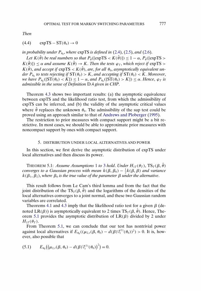
Then
expTS − ST(θ0)→ 0(4.4)
in probability under Pθ0 , where expTS is defined in (2.4), (2.5), and (2.6).Let K(θ̂) be real numbers so that Pθ̂([expTS <K(θ̂)]) ≤ 1 − α, Pθ̂([expTS >
K(θ̂)]) ≤ α and assume K(θ̂) → K. Then the tests ϕT , which reject if expTS >
K(θ̂), and accept if expTS <K(θ̂), are, for all θ0, asymptotically equivalent un-der Pθ0 to tests rejecting if ST(θ0) > K, and accepting if ST(θ0) < K. Moreover,we have Pθ0([ST(θ0) < K]) ≤ 1 − α, and Pθ0([ST(θ0) > K]) ≤ α. Hence, ϕT isadmissible in the sense of Definition D.4 given in CHP.
Theorem 4.3 shows two important results: (a) the asymptotic equivalencebetween expTS and the likelihood ratio test, from which the admissibility ofexpTS can be inferred, and (b) the validity of the asymptotic critical valueswhere θ̂ replaces the unknown θ0. The admissibility of the sup test could beproved using an approach similar to that of Andrews and Ploberger (1995).
The restriction to prior measures with compact support might be a bit re-strictive. In most cases, we should be able to approximate prior measures withnoncompact support by ones with compact support.
5. DISTRIBUTION UNDER LOCAL ALTERNATIVES AND POWER
In this section, we first derive the asymptotic distribution of expTS underlocal alternatives and then discuss its power.
THEOREM 5.1: Assume Assumptions 1 to 3 hold. Under H1T (θT ), TST (β� θ̂)converges to a Gaussian process with mean k(β�β0) − 1
2k(β�β) and variancek(β1�β2), where β0 is the true value of the parameter β under the alternative.
This result follows from Le Cam’s third lemma and from the fact that thejoint distribution of the TST (β� θ̂) and the logarithms of the densities of thelocal alternatives converges to a joint normal, and these two Gaussian randomvariables are correlated.
Theorems 4.1 and 4.3 imply that the likelihood ratio test for a given β (de-noted LR(β)) is asymptotically equivalent to 2 times TST (β� θ̂). Hence, The-orem 5.1 provides the asymptotic distribution of LR(β) divided by 2 underH1T (θT ).
From Theorem 5.1, we can conclude that our test has nontrivial poweragainst local alternatives if Eθ0((μ2�t(β�θ0) − d(β)′l(1)t (θ0))
2) > 0. It is, how-ever, also possible that
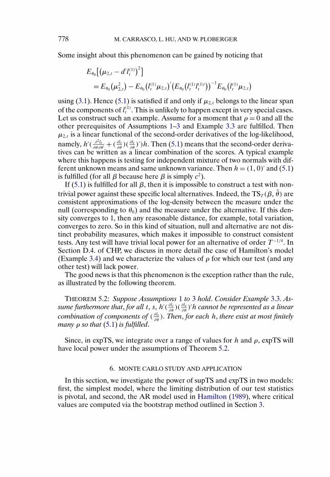
Eθ0
((μ2�t(β�θ0)− d(β)′l(1)t (θ0)
)2) = 0�(5.1)
778 M. CARRASCO, L. HU, AND W. PLOBERGER
Some insight about this phenomenon can be gained by noticing that
Eθ0
[(μ2�t − d′l(1)t
)2]=Eθ0
(μ2
2�t
) −Eθ0
(l(1)t μ2�t
)′(Eθ0
(l(1)t l(1)′t
))−1Eθ0
(l(1)t μ2�t
)using (3.1). Hence (5.1) is satisfied if and only if μ2�t belongs to the linear spanof the components of l(1)t . This is unlikely to happen except in very special cases.Let us construct such an example. Assume for a moment that ρ= 0 and all theother prerequisites of Assumptions 1–3 and Example 3.3 are fulfilled. Thenμ2�t is a linear functional of the second-order derivatives of the log-likelihood,namely, h′( ∂2lt
∂θ∂θ′ + ( ∂lt∂θ)( ∂lt
∂θ)′)h. Then (5.1) means that the second-order deriva-
tives can be written as a linear combination of the scores. A typical examplewhere this happens is testing for independent mixture of two normals with dif-ferent unknown means and same unknown variance. Then h= (1�0)′ and (5.1)is fulfilled (for all β because here β is simply c2).
If (5.1) is fulfilled for all β, then it is impossible to construct a test with non-trivial power against these specific local alternatives. Indeed, the TST (β� θ̂) areconsistent approximations of the log-density between the measure under thenull (corresponding to θ0) and the measure under the alternative. If this den-sity converges to 1, then any reasonable distance, for example, total variation,converges to zero. So in this kind of situation, null and alternative are not dis-tinct probability measures, which makes it impossible to construct consistenttests. Any test will have trivial local power for an alternative of order T−1/4. InSection D.4. of CHP, we discuss in more detail the case of Hamilton’s model(Example 3.4) and we characterize the values of ρ for which our test (and anyother test) will lack power.
The good news is that this phenomenon is the exception rather than the rule,as illustrated by the following theorem.
THEOREM 5.2: Suppose Assumptions 1 to 3 hold. Consider Example 3.3. As-sume furthermore that, for all t, s, h′( ∂lt
∂θ)( ∂ls
∂θ)′h cannot be represented as a linear
combination of components of ( ∂lt∂θ). Then, for each h, there exist at most finitely
many ρ so that (5.1) is fulfilled.
Since, in expTS, we integrate over a range of values for h and ρ, expTS willhave local power under the assumptions of Theorem 5.2.
6. MONTE CARLO STUDY AND APPLICATION
In this section, we investigate the power of supTS and expTS in two models:first, the simplest model, where the limiting distribution of our test statisticsis pivotal, and second, the AR model used in Hamilton (1989), where criticalvalues are computed via the bootstrap method outlined in Section 3.
OPTIMAL TEST FOR MARKOV SWITCHING PARAMETERS 779
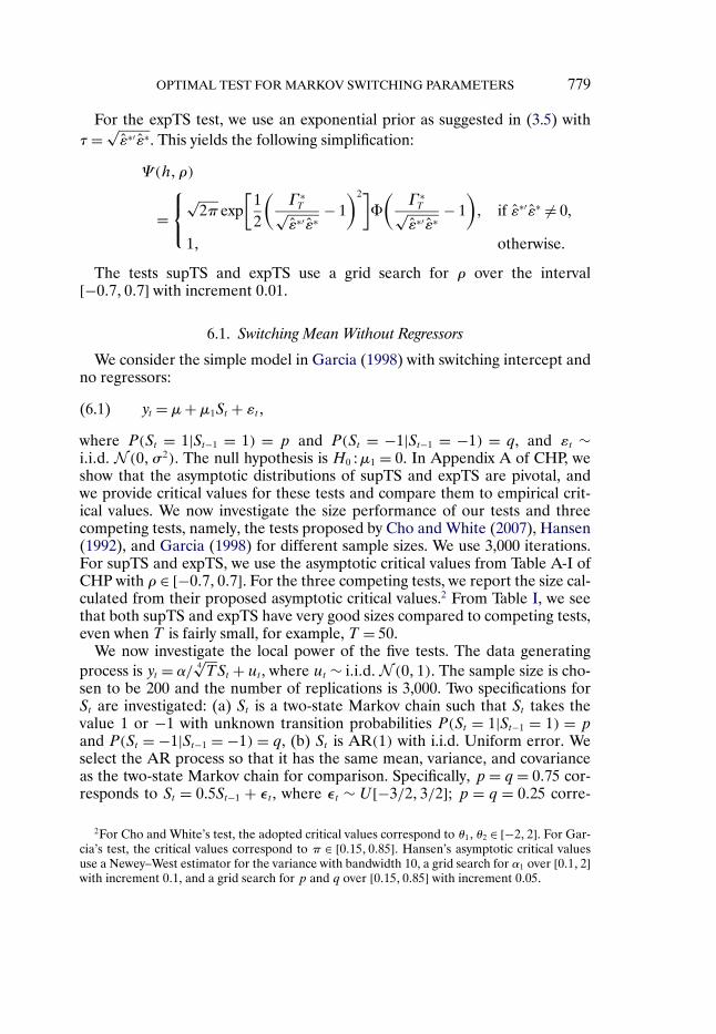
For the expTS test, we use an exponential prior as suggested in (3.5) withτ = √
ε̂∗′ε̂∗. This yields the following simplification:
Ψ(h�ρ)
=⎧⎨⎩
√2π exp
[12
(Γ ∗T√
ε̂∗′ε̂∗− 1
)2]�
(Γ ∗T√
ε̂∗′ε̂∗− 1
)� if ε̂∗′ε̂∗ = 0,
1� otherwise.
The tests supTS and expTS use a grid search for ρ over the interval[−0�7�0�7] with increment 0�01.
6.1. Switching Mean Without Regressors
We consider the simple model in Garcia (1998) with switching intercept andno regressors:
yt = μ+μ1St + εt�(6.1)
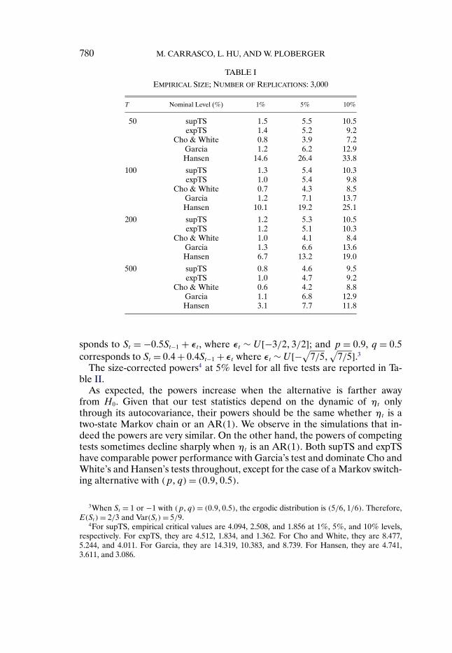
where P(St = 1|St−1 = 1) = p and P(St = −1|St−1 = −1) = q, and εt ∼i�i�d� N (0�σ2). The null hypothesis is H0 :μ1 = 0. In Appendix A of CHP, weshow that the asymptotic distributions of supTS and expTS are pivotal, andwe provide critical values for these tests and compare them to empirical crit-ical values. We now investigate the size performance of our tests and threecompeting tests, namely, the tests proposed by Cho and White (2007), Hansen(1992), and Garcia (1998) for different sample sizes. We use 3,000 iterations.For supTS and expTS, we use the asymptotic critical values from Table A-I ofCHP with ρ ∈ [−0�7�0�7]. For the three competing tests, we report the size cal-culated from their proposed asymptotic critical values.2 From Table I, we seethat both supTS and expTS have very good sizes compared to competing tests,even when T is fairly small, for example, T = 50.
We now investigate the local power of the five tests. The data generatingprocess is yt = α/
4√TSt + ut , where ut ∼ i�i�d� N (0�1). The sample size is cho-
sen to be 200 and the number of replications is 3,000. Two specifications forSt are investigated: (a) St is a two-state Markov chain such that St takes thevalue 1 or −1 with unknown transition probabilities P(St = 1|St−1 = 1) = pand P(St = −1|St−1 = −1) = q, (b) St is AR(1) with i.i.d. Uniform error. Weselect the AR process so that it has the same mean, variance, and covarianceas the two-state Markov chain for comparison. Specifically, p = q = 0�75 cor-responds to St = 0�5St−1 + εt , where εt ∼ U[−3/2�3/2]; p = q = 0�25 corre-
2For Cho and White’s test, the adopted critical values correspond to θ1� θ2 ∈ [−2�2]. For Gar-cia’s test, the critical values correspond to π ∈ [0�15�0�85]. Hansen’s asymptotic critical valuesuse a Newey–West estimator for the variance with bandwidth 10, a grid search for α1 over [0�1�2]with increment 0�1, and a grid search for p and q over [0�15�0�85] with increment 0�05.
780 M. CARRASCO, L. HU, AND W. PLOBERGER
TABLE I
EMPIRICAL SIZE; NUMBER OF REPLICATIONS: 3,000
T Nominal Level (%) 1% 5% 10%
50 supTS 1�5 5�5 10�5expTS 1�4 5�2 9�2
Cho & White 0�8 3�9 7�2Garcia 1�2 6�2 12�9Hansen 14�6 26�4 33�8
100 supTS 1�3 5�4 10�3expTS 1�0 5�4 9�8
Cho & White 0�7 4�3 8�5Garcia 1�2 7�1 13�7Hansen 10�1 19�2 25�1
200 supTS 1�2 5�3 10�5expTS 1�2 5�1 10�3
Cho & White 1�0 4�1 8�4Garcia 1�3 6�6 13�6Hansen 6�7 13�2 19�0
500 supTS 0�8 4�6 9�5expTS 1�0 4�7 9�2
Cho & White 0�6 4�2 8�8Garcia 1�1 6�8 12�9Hansen 3�1 7�7 11�8
sponds to St = −0�5St−1 + εt , where εt ∼ U[−3/2�3/2]; and p = 0�9, q = 0�5corresponds to St = 0�4 + 0�4St−1 + εt where εt ∼ U[−√
7/5�√
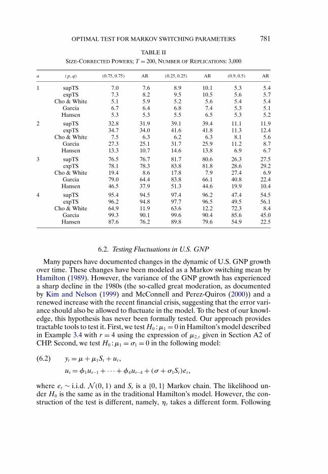
7/5].3The size-corrected powers4 at 5% level for all five tests are reported in Ta-
ble II.As expected, the powers increase when the alternative is farther away
from H0. Given that our test statistics depend on the dynamic of ηt onlythrough its autocovariance, their powers should be the same whether ηt is atwo-state Markov chain or an AR(1). We observe in the simulations that in-deed the powers are very similar. On the other hand, the powers of competingtests sometimes decline sharply when ηt is an AR(1). Both supTS and expTShave comparable power performance with Garcia’s test and dominate Cho andWhite’s and Hansen’s tests throughout, except for the case of a Markov switch-ing alternative with (p�q) = (0�9�0�5).
3When St = 1 or −1 with (p�q) = (0�9�0�5), the ergodic distribution is (5/6�1/6). Therefore,E(St)= 2/3 and Var(St) = 5/9.
4For supTS, empirical critical values are 4.094, 2.508, and 1.856 at 1%, 5%, and 10% levels,respectively. For expTS, they are 4.512, 1.834, and 1.362. For Cho and White, they are 8.477,5.244, and 4.011. For Garcia, they are 14.319, 10.383, and 8.739. For Hansen, they are 4.741,3.611, and 3.086.
OPTIMAL TEST FOR MARKOV SWITCHING PARAMETERS 781
TABLE II
SIZE-CORRECTED POWERS; T = 200, NUMBER OF REPLICATIONS: 3,000
α (p�q) (0�75�0�75) AR (0�25�0�25) AR (0�9�0�5) AR
Many papers have documented changes in the dynamic of U.S. GNP growthover time. These changes have been modeled as a Markov switching mean byHamilton (1989). However, the variance of the GNP growth has experienceda sharp decline in the 1980s (the so-called great moderation, as documentedby Kim and Nelson (1999) and McConnell and Perez-Quiros (2000)) and arenewed increase with the recent financial crisis, suggesting that the error vari-ance should also be allowed to fluctuate in the model. To the best of our knowl-edge, this hypothesis has never been formally tested. Our approach providestractable tools to test it. First, we test H0 :μ1 = 0 in Hamilton’s model describedin Example 3.4 with r = 4 using the expression of μ2�t given in Section A2 ofCHP. Second, we test H0 :μ1 = σ1 = 0 in the following model:
yt = μ+μ1St + ut�(6.2)
ut =φ1ut−1 + · · · +φ4ut−4 + (σ + σ1St)et�
where et ∼ i�i�d� N (0�1) and St is a {0�1} Markov chain. The likelihood un-der H0 is the same as in the traditional Hamilton’s model. However, the con-struction of the test is different, namely, ηt takes a different form. Following
782 M. CARRASCO, L. HU, AND W. PLOBERGER
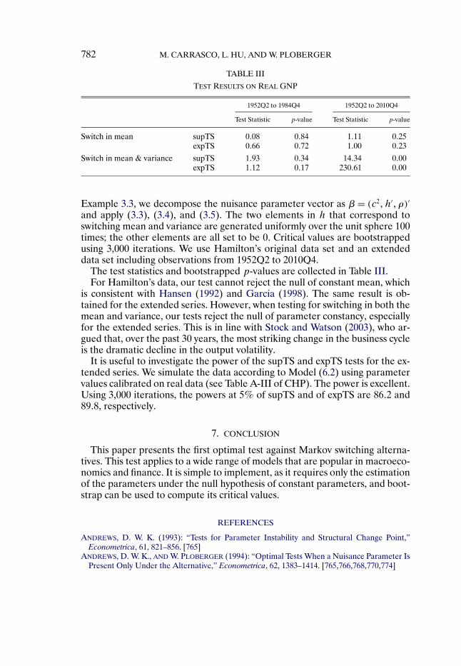
TABLE III
TEST RESULTS ON REAL GNP
1952Q2 to 1984Q4 1952Q2 to 2010Q4
Test Statistic p-value Test Statistic p-value
Switch in mean supTS 0�08 0�84 1�11 0�25expTS 0�66 0�72 1�00 0�23
Switch in mean & variance supTS 1�93 0�34 14�34 0�00expTS 1�12 0�17 230�61 0�00
Example 3.3, we decompose the nuisance parameter vector as β = (c2�h′�ρ)′
and apply (3.3), (3.4), and (3.5). The two elements in h that correspond toswitching mean and variance are generated uniformly over the unit sphere 100times; the other elements are all set to be 0. Critical values are bootstrappedusing 3,000 iterations. We use Hamilton’s original data set and an extendeddata set including observations from 1952Q2 to 2010Q4.
The test statistics and bootstrapped p-values are collected in Table III.For Hamilton’s data, our test cannot reject the null of constant mean, which
is consistent with Hansen (1992) and Garcia (1998). The same result is ob-tained for the extended series. However, when testing for switching in both themean and variance, our tests reject the null of parameter constancy, especiallyfor the extended series. This is in line with Stock and Watson (2003), who ar-gued that, over the past 30 years, the most striking change in the business cycleis the dramatic decline in the output volatility.
It is useful to investigate the power of the supTS and expTS tests for the ex-tended series. We simulate the data according to Model (6.2) using parametervalues calibrated on real data (see Table A-III of CHP). The power is excellent.Using 3,000 iterations, the powers at 5% of supTS and of expTS are 86�2 and89�8, respectively.
7. CONCLUSION
This paper presents the first optimal test against Markov switching alterna-tives. This test applies to a wide range of models that are popular in macroeco-nomics and finance. It is simple to implement, as it requires only the estimationof the parameters under the null hypothesis of constant parameters, and boot-strap can be used to compute its critical values.
REFERENCES
ANDREWS, D. W. K. (1993): “Tests for Parameter Instability and Structural Change Point,”Econometrica, 61, 821–856. [765]
ANDREWS, D. W. K., AND W. PLOBERGER (1994): “Optimal Tests When a Nuisance Parameter IsPresent Only Under the Alternative,” Econometrica, 62, 1383–1414. [765,766,768,770,774]
(1995): “Admissibility of the Likelihood Ratio Test When a Nuisance Parameter isPresent Only Under the Alternative,” The Annals of Statistics, 23, 1609–1629. [777]
BARTLETT, M. S. (1953a): “Approximate Confidence Intervals,” Biometrika, 40, 12–19. [770](1953b): “Approximate Confidence Intervals, II. More Than One Parameter,”
Biometrika, 40, 306–317. [770]BAUM, L., AND T. PETRIE (1966): “Statistical Inference for Probabilistic Functions of Finite State
Markov Chains,” Annals of Mathematical Statistics, 37, 1554–1563. [765]CARRASCO, M., L. HU, AND W. PLOBERGER (2014): “Supplement to ‘Optimal Test for
CHESHER, A. (1984): “Testing for Neglected Heterogeneity,” Econometrica, 52, 865–872. [766,770]
CHO, J. S., AND H. WHITE (2007): “Testing for Regime Switching,” Econometrica, 75, 1671–1720.[766,774,779]
COX, D. R., AND H. D. MILLER (1965): The Theory of Stochastic Processes. London: Methuen.[772]
DAVIDSON, R., AND J. MACKINNON (1991): “Une nouvelle forme du test de la matriced’information,” Annales d’Economie et de Statistique, 20/21, 171–192. [770]
(2004): Econometric Theory and Methods. New York: Oxford University Press. [771,773]DAVIES, R. B. (1977): “Hypothesis Testing When a Nuisance Parameter Is Present Only Under
the Alternatives,” Biometrika, 64, 247–254. [765](1987): “Hypothesis Testing When a Nuisance Parameter Is Present Only Under the
Alternatives,” Biometrika, 74, 33–43. [765,769]DOUKHAN, P. (1994): Mixing: Properties and Example. New York: Springer-Verlag. [772]DUFRÉNOT, G., V. MIGNON, AND A. PÉGUIN-FEISSOLLE (2011): “The Effects of the Subprime
Crisis on the Latin American Financial Markets: An Empirical Assessment,” Economic Mod-elling, 28, 2342–2357. [767]
GARCIA, R. (1998): “Asymptotic Null Distribution of the Likelihood Ratio Test in Markov Switch-ing Models,” International Economic Review, 39, 763–788. [766,779,782]
GONG, F., AND R. S. MARIANO (1997): “Testing Under Non-Standard Conditions in FrequencyDomain: With Applications to Markov Regime Switching Models of Exchange Rates and theFederal Funds Rate,” Staff Report 23, Federal Reserve Bank of New York. [766,774]
HALL, P. (1992): The Bootstrap and Edgeworth Expansion. New York: Springer-Verlag. [771]HAMILTON, J. D. (1989): “A New Approach to the Economic Analysis of Nonstationary Time
Series and the Business Cycle,” Econometrica, 57, 357–384. [765,773,778,781](2005): “What’s Real About the Business Cycle?” Federal Reserve Bank of St. Louis
Review, 87, 435–452. [767]HANSEN, B. (1992): “The Likelihood Ratio Test Under Non-Standard Conditions: Testing the
Markov Switching Model of GNP,” Journal of Applied Econometrics, 7, 61–82. [766,779,782](1996): “Inference When a Nuisance Parameter Is Not Identified Under the Null Hy-
pothesis,” Econometrica, 64, 413–430. [766]HU, L. (2011): “Optimal Test for Stochastic Unit Root With Markov Switching,” Report, Wayne
State University. [768]HU, L., AND Y. SHIN (2008): “Optimal Testing for Markov Switching GARCH Models,” Studies
in Nonlinear Dynamics and Econometrics, 12 (3), Article 3. [767]KAHN, J. A., AND R. W. RICH (2007): “Tracking the New Economy: Using Growth Theory to
Detect Changes in Trend Productivity,” Journal of Monetary Economics, 54, 1670–1701. [767]KIM, C. J., AND C. NELSON (1999): “Has the U.S. Economy Become More Stable? A Bayesian
Approach Based on a Markov-Switching Model of the Business Cycle,” The Review of Eco-nomics and Statistics, 81, 608–616. [781]
(2001): “A Bayesian Approach to Testing for Markov Switching in Univariate and Dy-namic Factor Models,” International Economic Review, 42, 989–1013. [766]
KUNITA, H. (1990): Stochastic Flows and Stochastic Differential Equations. Cambridge: CambridgeUniversity Press. [768]
LEE, L. F., AND A. CHESHER (1986): “Specification Testing When Score Test Statistics Are Iden-tically Zero,” Journal of Econometrics, 31, 121–149. [766,774]
MCCONNELL, M., AND G. PEREZ-QUIROS (2000): “Output Fluctuations in the United States:What Has Changed Since the Early 1980’s?” American Economic Review, 90, 1464–1476. [781]
MORLEY, J., AND J. PIGER (2012): “The Asymmetric Business Cycle,” The Review of Economicsand Statistics, 94, 208–221. [767]
STOCK, J., AND M. WATSON (2003): “Has the Business Cycle Changed and Why?” in NBERMacroeconomics Annual. Chicago: University of Chicago, 159–218. [782]
WALD, A. (1943): “Tests of Statistical Hypotheses Concerning Several Parameters When theNumber of Observations Is Large,” Transactions of the American Mathematical Society, 54,426–482. [774]
WARNE, A., AND A. VREDIN (2006): “Unemployment and Inflation Regimes,” Studies in Nonlin-ear Dynamics and Econometrics, 10 (2), 1–52. [767]
WHITE, H. (1982): “Maximum Likelihood Estimation of Misspecified Models,” Econometrica,50, 1–25. [766,770]
Département de Sciences Economiques, University of Montreal, CP 6128,succ Centre Ville, Montréal, Quebec H3C3J7, Canada; [email protected],
Dept. of Economics, Wayne State University, 656 W. Kirby St., Detroit, MI48202, U.S.A.; [email protected],
andDept. of Economics, Washington University in St. Louis, Campus Box 1208, St.