86
Jos´ e A. Carrillo Optimal Transport and Partial Differential Equations Mathematical Institute, Notes MT21

Jose A. Carrillo
Optimal Transportand
Partial Differential Equations
Mathematical Institute, Notes MT21


Preface
This course will serve as an introduction to optimal transportation theory, its appli-cation in the analysis of PDE, and its connections to the macroscopic description ofinteracting particle systems. The optimal transportation problem started with Gas-pard Monge in late XVIII century with his seminal work “Memoire sur la theoriedes deblais et des remblais” and expanded by Leonid Kantorovich with connectionsto economics. Brenier’s dynamical formulation of optimal transport in the 80’s-90’sgave rise to a flurry of applications of optimal mass transportation theory in PDEtheory, geometry, engineering, and lately in data science, that has been increasing inthe last 30 years. This course will cover some of the basic notions of transportationmetrics between probability measures as well as applications in mean-field limitsand PDE as gradient flows or steepest descent in spaces of probability measures.
The main learning outcomes are: Getting familiar with the Monge-Kantorovichproblem and transport distances. Derivation of macroscopic models via the mean-field limit and their analysis based on stability of transport distances. Dynamic In-terpretation and Geodesic convexity. A brief introduction to gradient flows and ex-amples. Prerequisites: A4 Integration. The short option in Calculus of Variation inPart A and functional analysis courses will ease understanding concepts but notcompulsory.
Regarding textbooks to find basic material I advice to look up the general mono-graphs in optimal transport theory [21, 18], the book [12] for basic related materialin functional analysis, the lecture notes from summer schools [11, 2, 8], and finally[14] for the mean-field limit and [20] for nonlinear diffusions. Additional materialcan be found related to courses taught at University of Cambridge [19] and at ETH-Zurich [13]. Further complementary material can also be found in [22, 4, 3].
v

Contents
1 Interacting Particle Systems & PDE . . . . . . . . . . . . . . . . . . . . . . . . . . . . . . 11.1 Aggregation Equation: Granular Flow Models. . . . . . . . . . . . . . . . . . . 11.2 Aggregation-Diffusion: McKean-Vlasov Equations. . . . . . . . . . . . . . . 41.3 Nonlinear Diffusions. . . . . . . . . . . . . . . . . . . . . . . . . . . . . . . . . . . . . . . . 61.4 Nonlinear Aggregation-Diffusion Equations: The Patlak-Keller-
Segel model. . . . . . . . . . . . . . . . . . . . . . . . . . . . . . . . . . . . . . . . . . . . . . . 91.5 Nonlinear Aggregation-Diffusion Equations: Phase Transitions in
collective behavior models. . . . . . . . . . . . . . . . . . . . . . . . . . . . . . . . . . . 11
2 Optimal Transportation: The metric side . . . . . . . . . . . . . . . . . . . . . . . . . 132.1 Functional Analysis tools: measures and weak convergence. . . . . . . . 132.2 A brief introduction to optimal transport . . . . . . . . . . . . . . . . . . . . . . . 152.3 The Kantorovich Formulation and Duality. The Brenier Theorem. . . 182.4 Transport distances between measures: properties. . . . . . . . . . . . . . . 292.5 One-dimensional Wasserstein metric . . . . . . . . . . . . . . . . . . . . . . . . . . 36
3 Mean Field Limit & Couplings . . . . . . . . . . . . . . . . . . . . . . . . . . . . . . . . . . 433.1 Measures sliding down a convex potential . . . . . . . . . . . . . . . . . . . . . . 433.2 Dobrushin approach: existence, stability, and derivation of the
Aggregation Equation. . . . . . . . . . . . . . . . . . . . . . . . . . . . . . . . . . . . . . . 473.3 Boltzmann Equation in the Maxwellian approximation: Tanaka
Theorem. . . . . . . . . . . . . . . . . . . . . . . . . . . . . . . . . . . . . . . . . . . . . . . . . . 54
4 An introduction to Gradient Flows . . . . . . . . . . . . . . . . . . . . . . . . . . . . . . . 614.1 Brenier’s Theorem and Dynamic Interpretation of optimal transport. 614.2 McCann’s Displacement Convexity: Internal, Interaction and
Confinement Energies. . . . . . . . . . . . . . . . . . . . . . . . . . . . . . . . . . . . . . . 634.3 Gradient Flows: the differential viewpoint. . . . . . . . . . . . . . . . . . . . . . 684.4 Gradient Flows: the metric viewpoint . . . . . . . . . . . . . . . . . . . . . . . . . . 72References . . . . . . . . . . . . . . . . . . . . . . . . . . . . . . . . . . . . . . . . . . . . . . . . . . . . . 79
vii


Chapter 1Interacting Particle Systems & PDE
This course is devoted to the analysis of solutions of the following family of PartialDifferential Equations
∂ρ
∂ t= ∇ · [ρ∇(V +W ∗ρ)]+∆P(ρ), (1.1)
where the unknown ρ(t, ·) is a time-dependent probability measure on Rd (d ≥ 1),P : [0,∞)→ R is an increasing function with P(0) = 0, V : Rd → R is a confine-ment potential and W : Rd → R is an interaction potential. The symbols ∇ and ∆
denote the gradient and the Laplacian operators and will always be applied to func-tions, while ∇· stands for the divergence operator, and will always be applied tovector fields. In the sequel, we identify both the probability measure ρ(t, ·) = ρtwith its Radon-Nikodym density dρt/dx with respect to Lebesgue, and thus, we usethe notation dρt = dρ(t,x) = ρ(t,x)dx unless discussing about general probabilitymeasures. The basic assumptions on P implies that the last term in (1.1) representsa diffusion term. The interaction potential W is always assumed to be symmetric:∀z ∈Rd , W (−z) =W (z). Finally, the smoothness on the potentials V and W will bespecified in each particular case.
We will be interested in understanding the well-posednes and the qualitativeproperties of solutions to (1.1) given by curves of probability densities, i.e., we arelooking for solutions such that ρ(t, ·) ∈ L1
+(Rd) for all t ≥ 0, and even sometimeswe will work with curves of probability measures. Sometimes in particular modelsthe measures will not be normalized to unit mass, but we will be assuming that welook for nonnegative integrable solutions with a fixed given mass.
1.1 Aggregation Equation: Granular Flow Models.
Rapid granular flow models were developed to describe dissipative or inelastic col-lisions between particles by statistical mechanic approaches. A basic model that
1

2 1 Interacting Particle Systems & PDE
triggered the attention of researchers in kinetic theory at the end of the 90’s on thistype of equations (1.1) with P = 0 can be introduced on the real line. Assume wehave particles on the real line moving freely until they collide, while they loose partof the relative velocity in each collision. Denopting by v and w the velocities ofthese particle before collision, and assuming conservation of the momentum but aloss of their relative velocity measured by the restitution coefficient 0 ≤ r ≤ 1, wecan write the post-collisional velocities by
v′ =12(v+w)+
r2(v−w); w′ =
12(v+w)− r
2(v−w). (1.2)
A more suitable form of (1.2) can be obtained by setting the coefficient of restitutionr = 1− 2r, where now 0 ≤ r ≤ 1/2 is the dissipation parameter. In terms of r, thedissipative collision reads
v′ = (1− r)v+ rw; w′ = rv+(1− r)w. (1.3)
Note that r = 1 corresponds to elastic collisions that in one dimension leads to triv-ial dynamics, swapping of labels for the particles. An integral equation given theevolution of the statistical distribution of the velocities of the particles on the linecan be phenomenologically introduced of the form
∂ f∂ t
+ v∂ f∂x
= Qr( f , f ), (1.4)
usually called a Boltzmann type equation, where the unknown is the statistical dis-tribution f (t,x,v) in position x and velocity v at time t ≥ 0. The right hand sidemodels the gain and loss of particles with a given velocity v due to collisions withother particles. The dissipative Boltzmann collision operator Qr( f , f ) is usually de-fined in its weak form, that is, in how it acts on given test functions ϕ ∈C∞(R)
< ϕ,Qr( f , f )>=∫R
∫R
B(|v−w|) f (v) f (w)[ϕ(v′)−ϕ(v)
]dvdw, (1.5)
with B(z), z ∈ [0,∞), being the collision frequency, i. e., the probability of collisionof two particles may depend on the relative velocity at which they are colliding.Typical values of the collision frequency are B(z) = |z|γ with γ ≥ −1, being γ = 1refered as inelastic hard spheres.
Notice that in order for the right hand side in (1.5) to be well defined, f must be-long to some Lp spaces and satisfy certain moments in v bounded depending on thegrowth of the test functions, but we proceed formally in order to understand furtherthe model. As mentioned earlier, in one–dimension of velocity space an elastic bi-nary collision particles simply exchange their velocities and the Bolzmann collisionoperator for elastic collisions disappears Q1 = 0. By the symmetry of the collisionmechanism (1.3), we can write the collision operator as

1.1 Aggregation Equation: Granular Flow Models. 3
<ϕ,Qr( f , f )>=12
∫R
∫R
B(|v−w|) f (v) f (w)[ϕ(v′)+ϕ(w′)−ϕ(v)−ϕ(w)
]dvdw.
(1.6)Let us now focus on the homogeneous problem, meaning that we assume the
initial data is homogeneous in space and we look for solutions only depending onthe velocity variable in order to understand just the velocity distribution, i.e., f (t,v)satisfies
∂ f∂ t
= Qr( f , f ). (1.7)
It is easy to check that the homogeneous Boltzmann equation conserves mass, mo-mentum and dissipates energy, meaning that
< 1,Qr( f , f )>=< v,Qr( f , f )>= 0
and
< v2,Qr( f , f )>=− (1− r)2
4
∫R
∫R
B(|v−w|)(v−w)2 f (v) f (w)dvdw.
These properties mean that solutions to (1.7) should be probability measures con-serving their mean and dissipating the kinetic energy by multiplying (1.7) by 1, vand v2 and integrating in v. Due to translational invariance, let us assume that themean velocity is zero, i.e., ∫
Rv f (t,v)dv = 0, ∀t ≥ 0. (1.8)
Let us look for simpler models, assuming that the inelasticity is small r ' 1 orequivalentely r' 0, we approximate the Boltzmann collision operator by expandingin the expression (1.5) to get
ϕ(v′)−ϕ(v)' ∂ϕ
∂v(v)(v′− v) =−r(v−w)
∂ϕ
∂v(v).
Therefore, we can approximate the collision operator Qr( f , f ) by
< ϕ,Qr( f , f )>'−r∫R
∫R
B(|v−w|)(v−w) f (v) f (w)∂ϕ
∂v(v)dvdw. (1.9)
The right-hand side of (1.9) is the weak form of a differential operator, thus we canfinally write a one-dimensional simplified granular flow model as
∂ f∂ t
=∂
∂v
[f(
∂W∂v∗ f)]
, with∂W∂v
= vB(|v|), (1.10)
where the factor r is absorbed in the time derivative. Notice that for the typical casesof collision frequencies, W (v) = |v|γ+2
γ+2 , γ ≥ −1. Therefore, this simplified granular
4 1 Interacting Particle Systems & PDE
flow model corresponds to cases of the general family of PDE (1.1) with V = 0,P = 0 and convex interaction potentials W .
Intuitively, we should expect concentration in velocity variable as time evolvesdue to the inelasticity of the interactions, particles will start to decrease their rela-tive velocities until eventually reaching rest state. Is this captured by the simplifiedmodel (1.10)? Let us look at the evolution of the variance of the distribution invelocity variable, that is
ddt
∫R|v|2 f (t,v)dv =−
∫R
∫R
B(|v−w|)(v−w)2 f (v) f (w)dvdw
by substituting in (1.9) and symetrizing. In case γ = 0, we can expand the squareand use the conservation of zero mean velocity (1.8) to simplify the right-handside. Therefore, denoting the variance of f (t, ·) by x(t), then it follows the ODEx′(t) ≤ −cx(t), and thus x(t)→ 0 as t → ∞ exponentially fast for γ = 0. We con-clude that the variance is decreasing and converging to 0 as t → ∞. Let us assumethat there is no concentration in finite time, as a consequence as t→∞ the probabil-ity densities f (t, ·) δ0 weakly-∗ as measures as t → ∞. Now the question is howthis concentration in velocity happens for the solutions of (1.10), does it really hap-pen in finite or infinite time and if so, can we understand the convergence towardsconcentration? Is there any typical profile? What is the long-time behavior for othervalues of −1≤ γ?
1.2 Aggregation-Diffusion: McKean-Vlasov Equations.
Consider a confinement potential V ∈C1, and a particle that moves in this potentialwith a large friction such that we can neglect the inertia term. Thus a given particleXt follow the ODE system dXt
dt =−∇V (Xt). Let us also assume that we perturb thismotion stochastically by a Brownian noise added to the system of strength σ . There-fore, the SDE system followed by the particle is given by the Langevin equation
dXt =−∇V (Xt)dt +√
2σ dBt , (1.11)
where Bt is the standard Brownian motion. Ito’s formula implies that the law ρ(t, ·)of the random variable Xt satisfies the Fokker-Planck equation
∂ρ
∂ t= ∇ · (ρ∇V )+σ∆ρ, (1.12)
that is a particular case of the general family of PDE (1.1) with general confinementpotential V , zero interaction W = 0 and linear diffusion P(ρ) = σρ . One can easilyobserve that convexity properties of V will play an important role in the long timedynamics of this equations (1.11) or equivalently (1.12). In fact, let us take tworealizations Xt and Yt , t ≥ 0, of the SDE (1.11), meaning two solutions of (1.11)with differential initial data but constructed with the same Brownian motion. This
1.2 Aggregation-Diffusion: McKean-Vlasov Equations. 5
means that the solutions Xt and Yt are correlated for t > 0 even if we assume theminitially independent. Since they are constructed from the same Brownian motion,even if separately both trajectories Xt and Yt do not have good regularity, it is notdifficult to deduce from stochastic analysis theory that the difference αt = Xt−Yt isC1, and it satisfies
dαt
dt=−(∇V (Xt)−∇V (Yt)), t ≥ 0,
and therefore, we deduce
12
ddt|αt |2 =−(∇V (Xt)−∇V (Yt)) · (Xt −Yt), t ≥ 0.
Therefore, if the potential V is uniformly convex, there exists λ > 0 such that D2V ≥λ Id , then 1
2ddt |αt |2 ≤ −λ |αt |2, for all t ≥ 0, and thus |αt |2 ≤ |αt |2e−2λ t . Now, take
the initial random variables X0 and Y0 with finite variance, i.e., E[|X0|2] < ∞ andE[|Y0|2]< ∞, we can compute the expectation of |αt |2 as
E[|Xt −Yt |2]≤ E[|X0−Y0|2]e−2λ t ≤ 2(E[|X0|2 +E[|Y0|2]
)e−2λ t , t ≥ 0.
Therefore, two solutions of the SDE converge towards each other exponentially fastin the above sense. It is easy to check by direct inspection that the normalized Gaus-sian
ρ∞(x) =1Z
e−V (x)/σ with Z =∫Rd
e−V (x)/σ dx,
is a stationary state of (1.12). By taking Y0 the random variable whose distributionis given by ρ∞, we have shown that all solutions of the Langevin equation (1.11)converge in the sense above to the stationary state (1.11). The Gaussian measureρ∞ is usually referred as invariant measure in stochastic analysis. We will see howthis convergence translates onto the convergence of solutions ρ(t, ·) of the linearFokker-Planck equation (1.12) towards ρ∞ in a suitable sense.
Finally, we can also introduce a pairwise interaction potential W between parti-cles and introduce a systems of N interacting particles perturbed by Brownian noiseof the form
dX it =−
1N
N
∑i6= j
∇W (X it −X j
t )dt +√
2σ dBit , (1.13)
where Bit , i = 1, . . . ,N, are N independent Brownian motions. Now, it is more dif-
ficult to analyse the correlations between the particles and what is the PDE, if any,that gives the typical behavior of one of the particles as N→ ∞. The answer to thisquestion is the so-called mean-field limit that allows to identifiy the limiting PDEthat satisfies the law of a particle in the large number of particles limit N→ ∞. No-tice that the interaction potential has the factor 1
N in front in the SDE system (3.9),which is crucial to identify a sort of mean-field potential created by the particle en-

6 1 Interacting Particle Systems & PDE
semble. It is proven that under certain assumptions on the interaction potential thelimiting PDE is given by the McKean-Vlasov equation
∂ρ
∂ t= ∇ · [ρ(∇W ∗ρ)]+σ∆ρ. (1.14)
Convexity properties of the interaction potential will give information on the longtime asymptotics of both the SDE system (3.9) and the McKean-Vlasov equation(1.14). Let us finally remark that McKean-Vlasov equation (1.14) are ubiquitous inapplications in the sciences from sinchronysation to swarming models for collectivebehavior in mathematical biology, to opinion formation in social sciences or to self-assembly alloys and granular flows in material science, and lately they have founda renewed interest in data science.
1.3 Nonlinear Diffusions.
The most well-known cases of nonlinear diffusions are the homogeneus nonlineari-ties, P(ρ) = ρm with m> 0. The flow of gas in an d-dimensional porous medium isdescribed by Darcy’s law, pressure proportional to the density of the gas, leading to
∂u∂ t
= ∆um, (x ∈ Rd , t > 0), (1.15)
The function u represents the density of the gas in the porous medium and m > 1is a physical constant. This equation can be thought as a nonlinear heat equationin which the thermal conductivity is mρm−1, and therefore directly proportional tothe density for m> 1. The porous medium equation degenerates in vacuum, i.e. forρ = 0, leading to the interesting phenomena of free boundaries and finite speed ofpropagation due to slow diffusion for small values of the density. We refer to [20]for a comprehensive treatment of this problem. The equation for 0<m< 1 receivesthe name of fast diffusion equation since the heat conduction is now inversely pro-portional to the density, and thus very fast diffusion happens for small values of thedensity u.
Equation (1.15) has some important explicit solutions that led to the advance offunctional analysis and techniques for understading long-time behavior of nonlineardiffusion equations since the 1970’s. There are self-similar solutions generalizingthe role of the heat kernel for the heat equation. Let us remind that the solution tothe Cauchy problem for the heat equation
∂u∂ t
= σ∆u, (x ∈ Rd , t > 0), (1.16)
with initial data a probability measure ρ0 = µ can be obtained by the Poisson’sformula ρt = K(t, ·)∗µ donde K(t,x) is the heat kernel given by
1.3 Nonlinear Diffusions. 7
K(t,x) = (4πσt)−d2 exp
(− x2
4σt
). (1.17)
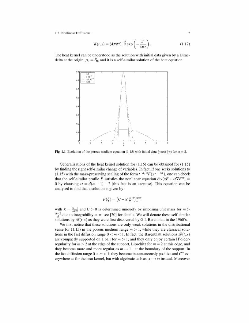
The heat kernel can be understood as the solution with initial data given by a Dirac-delta at the origin, ρ0 = δ0, and it is a self-similar solution of the heat equation.
−8 −6 −4 −2 0 2 4 6 80
0.1
0.2
0.3
0.4
0.5
0.6
0.7
0.8
x
t=0
t=10−1
t=5⋅ 10−1
t=20
Fig. 1.1 Evolution of the porous medium equation (1.15) with initial data π
4 cos( π
2 x) for m = 2.
Generalizations of the heat kernel solution for (1.16) can be obtained for (1.15)by finding the right self-similar change of variables. In fact, if one seeks solutions to(1.15) with the mass-preserving scaling of the form t−d/α F(xt−1/α), one can checkthat the self-similar profile F satisfies the nonlinear equation div(xF +α∇Fm) =0 by choosing α = d(m− 1) + 2 (this fact is an exercise). This equation can beanalysed to find that a solution is given by
F(ξ ) =(C−κ|ξ |2
) 1m−1+
with κ = m−12mα
and C > 0 is determined uniquely by imposing unit mass for m >d−2
d due to integrability at ∞, see [20] for details. We will denote these self-similarsolutions by B(t,x) as they were first discovered by G.I. Barenblatt in the 1960’s.
We first notice that these solutions are only weak solutions in the distributionalsense for (1.15) in the porous medium range m > 1, while they are classical solu-tions in the fast diffusion range 0 < m < 1. In fact, the Barenblatt solutions B(t,x)are compactly supported on a ball for m > 1, and they only enjoy certain H’older-regularity for m> 2 at the edge of the support, Lipschitz for m = 2 at this edge, andthey become more and more regular as m→ 1+ at the boundary of the support. Inthe fast diffusion range 0<m< 1, they become instantaneously positive and C∞ ev-erywhere as for the heat kernel, but with algebraic tails as |x|→∞ instead. Moreover
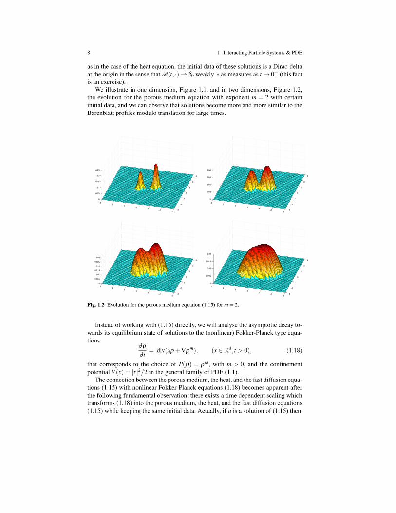
8 1 Interacting Particle Systems & PDE
as in the case of the heat equation, the initial data of these solutions is a Dirac-deltaat the origin in the sense that B(t, ·) δ0 weakly-∗ as measures as t→ 0+ (this factis an exercise).
We illustrate in one dimension, Figure 1.1, and in two dimensions, Figure 1.2,the evolution for the porous medium equation with exponent m = 2 with certaininitial data, and we can observe that solutions become more and more similar to theBarenblatt profiles modulo translation for large times.
−3
−2
−1
0
1
2
3
−3−2
−10
12
3
0
0.05
0.1
0.15
0.2
0.25
−3
−2
−1
0
1
2
3
−3−2
−10
12
3
0
0.02
0.04
0.06
0.08
−3
−2
−1
0
1
2
3
−3−2
−10
12
3
0
0.005
0.01
0.015
0.02
0.025
0.03
−3
−2
−1
0
1
2
3
−3−2
−10
12
3
0
0.005
0.01
0.015
0.02
Fig. 1.2 Evolution for the porous medium equation (1.15) for m = 2.
Instead of working with (1.15) directly, we will analyse the asymptotic decay to-wards its equilibrium state of solutions to the (nonlinear) Fokker-Planck type equa-tions
∂ρ
∂ t= div(xρ +∇ρ
m), (x ∈ Rd , t > 0), (1.18)
that corresponds to the choice of P(ρ) = ρm, with m > 0, and the confinementpotential V (x) = |x|2/2 in the general family of PDE (1.1).
The connection between the porous medium, the heat, and the fast diffusion equa-tions (1.15) with nonlinear Fokker-Planck equations (1.18) becomes apparent afterthe following fundamental observation: there exists a time dependent scaling whichtransforms (1.18) into the porous medium, the heat, and the fast diffusion equations(1.15) while keeping the same initial data. Actually, if u is a solution of (1.15) then
1.4 Nonlinear Aggregation-Diffusion Equations: The Patlak-Keller-Segel model. 9
ρ(t,x) = edtu(
eαt −1α
,et x)
(1.19)
is a solution of (1.18) and vice versa, if ρ is a solution of (1.18), then
u(t,x) = (1+αt)−d/αρ
(1α
log(
1+αt),(
1+αt)−1/α
x)
(1.20)
is a solution of (1.15) (these facts are an exercise). We finally remark that a stationarysolution of (1.18) is given by the Barenblatt type formula
ρ∞(x) =(
C− m−12m|x|2) 1
m−1
+
(1.21)
for a C> 0 such that ρ∞ has unit mass. In fact, one can check that this is a stationarysolution of (1.18) by noticing that the flux xρ +∇ρm is zero,
xρ∞ +∇ρm∞ = ρ∞
(m
m−1∇ρ
m−1∞ + x
)= 0.
Notice that the last computation makes sense since ρm−1∞ is a Lipschitz function.
We point out that ρ∞(x) corresponds to B(t + 1α,x) through the change of vari-
ables (1.19)–(1.20). As a conclusion, if we are able to derive any property aboutthe asymptotic behavior of ρ(t,x) towards ρ∞(x) we can translate it into a resultabout the asymptotic behavior of u(t,x) towards the Barenblatt profile B(t,x). Moreprecisely, showing the exponential decay of the solutions to (1.18) towards the sta-tionary state ρ∞ translates into algebraic decay towards self-similar profiles of theporous medium, the heat, and the fast diffusion equations (1.15) via the change ofvariables (1.19)–(1.20).
1.4 Nonlinear Aggregation-Diffusion Equations: ThePatlak-Keller-Segel model.
The Patlak-Keller-Segel (PKS) equation is widely used in mathematical biology tomodel the collective motion of cells which are attracted by a self-emitted chemi-cal substance, being the slime mold amoebae Dictyostelium discoideum a prototypeorganism for this behaviour. Moreover, the PKS equation has become a paradig-matic mathematical problem since it shows a concentration-collapse dichotomy: formasses larger than a critical value solutions aggregate their mass, as Dirac-deltas, infinite time while solutions exist globally and disperse collapsing down to zero belowthis critical mass threshold.
Historically, the first mathematical models in chemotaxis were introduced in1953 by C. S. Patlak and E. F. Keller and L. A. Segel in 1970 in two dimensionssince they were interested in the chemotactic movement of cells in Petri dishes. The

10 1 Interacting Particle Systems & PDE
basic model in any dimension reads as∂ρ
∂ t= ∆ρ−χ∇·[ρ∇c] t > 0 , x ∈ Rd ,
c(t,x) =− 1dπ
∫Rd
log |x− y|ρ(t,y)dy , t > 0 , x ∈ Rd ,(1.22)
Here (t,x) 7→ ρ(t,x) represents the normalized cell density, and (t,x) 7→ c(t,x) is theconcentration of chemo-attractant. The constant χ > 0 is the sensitivity of the bac-teria to the chemo-attractant. Mathematically, it measures the attractive interactionforce between cells, and hence, the strength of the non-linear coupling. Note that(1.22) corresponds to the choice P(ρ) = ρ and W (x) = − 1
dπlog |x| in the general
family of PDE (1.1).We first remind that a notion of weak solution ρ in the space C0
([0,T );L1
+(Rd)),
with fixed T > 0, using the symmetry in x, y for the concentration gradient, can beintroduced to handle even measure solutions. We shall say that ρ is a weak solutionto the system (1.22) if for all test functions ζ ∈C2
b(Rd),
ddt
∫Rd
ζ (x)ρ(t,x)dx =∫Rd
∆ζ (x)ρ(t,x)dx
− χ
2d π
∫∫Rd×Rd
[∇ζ (x)−∇ζ (y)] · x− y|x− y|2 ρ(t,s)ρ(t,y)dxdy (1.23)
in the distributional sense in (0,T ). Here, the Banach space C2b(Rd) is defined as the
set of C2-functions with bounded second derivatives. Notice that the singularity dueto the derivative of the log-kernel dissappears by symmetrization of the term usingthe mean value theorem. Any weak solution in the previous sense with initial data aprobability density function satisfies mass and center of mass conservations, i. e.,∫Rd
ρ(t,x) dx =∫Rd
ρ0(t,x) dx = 1 and∫Rd
xρ(t,x) dx =∫Rd
xρ0(t,x) dx = 0,
the latter being assumed without loss of generality by translational invariance. Inorder to check the behavior of the system, we can check the evolution of the varianceof the distribution as done in the first example of this section. By taking ζ (x) = |x|2as test function in (1.23), we obtain
ddt
∫Rd|x|2 ρ(t,x)dx = 2d− χ
d π.
Therefore, if χ > 2d2π , the variance of the distribution ρ(t,x) becomes zero in finitetime. This means that in finite time, there should be a concentration as a Dirac-deltaat the origin contradicting the existence of a weak solution in the sense of (1.23) atthat time.
This intuition can be made rigorous at certain extent. The Cauchy problem for thePKS equation (1.22) presents the following dichotomy: either L1-solutions blow-up

1.5 Nonlinear Aggregation-Diffusion Equations: Phase Transitions in collective behavior models.11
in finite time for the super-critical case χ > 2d2π or rather solutions exist globallyin time and spread in space decaying towards a stationary solution in rescaled vari-ables as t→ ∞ in the sub-critical case χ < 2d2π . The critical case χ = 2d2π is alsofairly well understood leading to infinite time blow-up or convergence to station-ary states depending on the initial data. We refer to the recent survey [9] and thereferences therein for further details and even more general cases with nonlineardiffusions and general interaction kernels. This example show us that concentrationand diffusion phenomena can coexist for the same type of equations depending onjust one parameter.
1.5 Nonlinear Aggregation-Diffusion Equations: PhaseTransitions in collective behavior models.
The final example arises in collective behavior models for animal swarming. Werefer to the survey [10] for details about the modelling and the mean-field limit frominteracting particle systems of 2nd order leading to the following localized Cucker-Smale model for aligment for self-propelled particles with noise. Here, f representsthe distribution in both space x and velocity v at time t of individuals, and the modelfeatures a Cucker-Smale term which aligns the velocity of points nearby in space, aterm adding noise in the velocity, and a friction term which relaxes velocities backto norm one leading to
∂ f∂ t
+ v ·∇x f = ∇v ·(β (|v|2−1)v f +(v−u f ) f +σ∇v f
),
where
u f (t,x) =∫
K(x,y)v f (t,y,v)dvdy∫K(x,y) f (t,y,v)dvdy
.
Here K(x,y) is a suitably defined compactly supported localization kernel and β andσ are respectively the self-propulsion force and noise intensities. If we first look forthe behavior in the spatially homogeneous case, the model reduces to
∂t f = ∇v ·(β (|v|2−1)v f +(v−u f ) f +σ∇v f
). (1.24)
whereu f (t) =
∫Rd
v f (t,v)dv, (1.25)
and where f = f (t,v) is the velocity distribution at time t. This alignment model canbe again recast as the general PDE (1.1) by the changing the notation from f (t,v) toρ(t,x) with the choices
P(ρ) = σρ, V (x) = β
(|x|44 −
|x|22
)and W (x) = |x|2
2 .

12 1 Interacting Particle Systems & PDE
The interesting phenomena happening in this particular model is that as soon as oneof the potentials, in this case the confinement potential, is not convex, complicateddynamics can happen. In fact, there is a phase transition between unpolarized andpolarized motion as the noise intensity σ is varied, for a specific range of the valuesof β . More precislely, one can analytically prove that, for large noise σ , there is onlyone isotropic stationary solution, while for small σ , there is an additional infinitefamily of stationary states parameterized by a unit vector on the sphere, referred toas the polarized equilibria. Moreover the change from one single isotropic stationarystate to infintely many steady states happens at a precise threshold critical valueof σc, depending on β , that is known in dimensions 1 and 2, see Fig. 1.3. Thesequestions are nowadays of current interest in research.
0 0.1 0.2 0.3 0.4 0.5 0.60
0.1
0.2
0.3
0.4
0.5
0.6
0.7
0.8
0.9
1
sigma (diffusion coefficient)
u (
magnitude o
f m
ean v
elo
city o
f sta
tionary
solu
tion)
Two dimensional bifurcation diagram
beta=1 beta=10beta=20 beta=40 beta=60 beta=80beta=100
Fig. 1.3 Mean speed u of the stationary state as a function of the diffusion parameter σ for severalvalues of the self-propulsion strength β . There is a continuous bifurcation critical diffusion σc fromthe existence of polarized to unpolarized stationary states.
Chapter 2Optimal Transportation: The metric side
In this chapter, we will do a short primer on the classical optimal transport and theirassociated transport distances. Let us start by introducing quickly the basic notationof the objects we are dealing with, probability mesures.
2.1 Functional Analysis tools: measures and weak convergence.
Let us consider the space of continuous functions with zero limit at infinity C0(Rd),i.e., f ∈ C0(Rd) if it is continuous and for all ε > 0, there exists R > 0 such that| f (x)| ≤ ε for |x| ≥R. C0(Rd) is a separable Banach space endowed with the uniformnorm. We recall a basic notion in measure theory
Definition 2.1. A finite signed measure µ on Rd is a map that assigns to every Borelsubset A⊂ Rd a value µ(A) ∈ R such that
µ (∪i≥1Ai) = ∑i≥1
µ (Ai) and ∑i≥1|µ (Ai) |< ∞
hold for every countable disjoint union Ai∩A j = /0, i 6= j. The set of all finite signedmeasures on Rd will be denoted by M (Rd). It is a Banach space endowed with thenorm
‖µ‖= sup
∑i≥1|µ (Ai) | : Rd = ∪i≥1Ai with Ai∩A j = /0, i 6= j
.
Riesz’s representation theorem provides a very useful characterization of the setof finite signed measures, every element of the dual Banach space X ′ of X =C0(Rd) can be represented in a unique way by a finite signed measure µ ∈M (Rd).The weak-∗ convergence on finite signed measures is then defined based on the dualpairing (C0(Rd),M (Rd)) and its representation
13
14 2 Optimal Transportation: The metric side
< µ,ϕ >=∫Rd
ϕ(x)dµ(x).
We say that the sequence of measures µn converges weakly-∗ to µ if and only if< µn,ϕ >→< µ,ϕ > for all ϕ ∈C0(Rd). This will be denoted by µn µ weakly-∗. In short, the dual space to C0(Rd) is by definition the set of locally finite signedRadon measures in Rd . The set of probability measures P(Rd) is defined as thesubset of nonnegative finite signed measures such that µ(Rd) = 1.
Let us denote by L the Lebesgue measure on Rd . When a probability measureµ ∈P(Rd) is absolutely continous with respect to the Lebesgue measure, that isit has at least the same zero measures sets, denoted by µ ÎL , then the measure µ
has a density ρ ∈ L1+(Rd), meaning that by the Radon-Nikodym theorem, it can be
represented by the density ρ , i. e.
< µ,ϕ >=∫Rd
ϕ(x)dµ(x) =∫Rd
ϕ(x)ρ(x)dx.
We will use in these set of notes the notation of measure and its associated density in-distinctively unless there is confusion. To finish these measure theory preliminaries,let us introduce another notion of convergence by duality for probability measures.We say that the sequence of measures µn narrow or weakly converges to µ if andonly if < µn,ϕ >→< µ,ϕ > for all ϕ ∈Cb(Rd) or in other words that the measuresconvergences in the duality with Cb(Rd). This will also be denoted abusing the no-tation by µn µ . We point out that the dual of Cb(Rd) can also be characterized interms of certain set of measures larger than M (Rd) but it is a weird space, see [21,Section 1.3] for further details.
Finally, let us remind few Functional Analysis results on the compactness ofsubsets of measures. Given a dual pair of Banach spaces (X ,X ′) and its associatedduality < ·, · >, Banach-Alaoglu’s theorem asserts that any bounded set in X ′ isprecompact in the weak-∗ topology. In practice, this implies that any sequence ofprobability measures has a weakly-∗ subsequence towards a nonnegative measurenot necessarily being a probability measure. In order for the weak-∗ limit to be aprobability measure, we need an additional property.
Definition 2.2. A sequence µn in P(Rd) is said to be tight if for every ε > 0, thereexists R > 0 such that µn(Rd \BR) ≤ ε for every n, where BR is the euclidean ballof radius R centered at the origin.
We refer to [6] for futher details on duality pairings and weak topologies.Prokhorov’s Theorem gives a characterization of weakly-∗ precompact subsets
of probability measures.
Theorem 2.1. (Prokhorov) Every tight sequence µn in P(Rd) has a weakly or nar-rowly convergent subsequence to a limiting probability measure. Conversely, everyweakly converging sequence of probability measures µn µ is tight.
In order to explain better the classical optimal transportation problem, we needsome further definitions.
2.2 A brief introduction to optimal transport 15
Definition 2.3. Let µ and ν be in P(Rd) the space of probability measure in Rd ,and T be a measurable map Rd → Rd . We say that T transports µ onto ν , ν is thepush-forward or the image measure of µ through T , and we denote it by ν = T #µ ,if for any measurable set B⊂ Rd , ν(B) = µ(T−1(B)).
In fact, the previous definition of pushforward is equivalent to∫Rd(ζ T )(x)dµ(x) =
∫Rd
ζ (y)dν(y) ∀ζ ∈ Cb(Rd) . (2.1)
Actually, the change of variables formula (2.1) is true for all ζ ∈ L1(Rd). We leavethis as a warm-up in integration, measure theory and dominated/monotone conver-gence theorems (this fact is an exercise). The image measure through a map T canalso be directly connected to basic probability theory. In fact, a random variable Xwith law µ is by definition a measurable map X : (S ,A ,P) −→L from a proba-bility space of reference (S ,A ,P) onto the Lebesgue space L such that the imagemeasures through X of P is µ , i.e. X#P = µ .
2.2 A brief introduction to optimal transport
Let us first introduce intuitively the optimal transportation problem. Let us assumethat the probability measure µ represents the density of frozen fish-and-chips sup-pliers in the United Kingdom while the probability measure ν represents the densityof pubs (it is a good approximation to assume that at least the measure ν has partswhich are absolutely continuous with respect to Lebesgue and atomic parts, thinkabout the London area or the Costwolds while the first measure µ might be con-centrated in coastal areas in the Southwest of England and Scotland). Assume thatthe market is in equilibrium, meaning supply=demand, so all the produced frozenfish-and-chips are consumed by the pubs. The question we want to solve is how tofind a way of transporting all the product from the suppliers at each specified loca-tion x to the the consumers at locations y optimally. The optimality here has to bespecified and it should include an estimate of the cost needed for the transportation.The union of frozen fish-and-chips suppliers is overseeing the whole operation oftransportation, thus they would like to know how to transport all the frozen fish-and-chips from the suppliers to the consumers minimizing the overall cost of thistask. Let us represent by c(x,y) the cost of sending a unit of the product from sup-plier location x ∈ Rd to consumer location y ∈ Rd , i.e., we define a cost functionc : Rd×Rd 7→ [0,∞).
The transportation problem was mathematically set up for the first time by Gas-pard Monge, a French mathematician and engineer in the late 1700’s in his essay“Memoire sur la theorie des deblais et remblais” in 1781. His transportation prob-lem was very much related to French army’s operations and less to fish-and-chipsdistribution though. He posed the problem in the following way, from all possibleways of transporting the goods from location x to location y, can we find the optimal

16 2 Optimal Transportation: The metric side
one minimizing the total incurred cost? More precisely and in modern mathemati-cal terms, given two probability measures µ and ν , can we find an optimal map Ttransporting µ onto ν , ν = T #µ , minimizing the total cost given by∫
Rdc(x,T (x))dµ(x)?
This classical problem from Calculus of Variation, sketched in Figure 2.1, is the
Fig. 2.1 Monge trasnportation problem between two probability measures µ0 and µ1. Figure takenfrom Wikipedia.
so-called Monge transportation problem, that is to find, if possible, the solution tothe following minimization problem:
IM := infT
∫Rd
c(x,T (x)dµ(x) : ν = T #µ
.
He posed this question with the cost given by the distance between the locationsc(x,y) = |x− y|. It is very easy to see that this problem does not have a solutionfor general probability measures. In fact, the set of maps pushing one probabil-ity measure µ onto ν might be even empty making the classical Monge problemtrivially impossible. Take µ = δx0 and ν = 1
2 δx0 +12 δx1 with x0 6= x1 where δx0 is
the Dirac delta measure at x0. Then ν(x1) = 12 but either µ(T−1(x1)) = 1 or
µ(T−1(x1)) = 0 depending if T (x0) = x1 or not. Thus, there is no map pushingforward µ onto ν .
The issue here is that in the classical Monge transportation problem choosingtransportation maps is not a good idea. It is a better idea “to split the mass”, thisis even more advantageous economically. In fact, Leonyd Kantorovich in 1942 re-alized that a better way to pose the transportation problems lies in the basic ideathat for each producer it will be generically more economic to split its productionamong several consumers that sending all its production to a unique location. Heintroduced the concept of transportation or transference plan, that is a probabilitymeasure Π(x,y) on the product space Rd ×Rd with marginals µ and ν . The basicmeaning of Π(x,y) is the number of units of production at location x sent to locationy while using fully the total number of produced units by the supplier located at xand fulfilling the total number of units demanded by the consumer located at y. Themathematical statement of the last sentence is translated in the fact that the marginalmeasures of Π must be µ and ν respectively. Let us denote by Γ (µ,ν) the set of
2.2 A brief introduction to optimal transport 17
all transference plans, that is, the set of joint probability measures on Rd×Rd withmarginals µ and ν , i.e.,∫∫
Rd×Rdϕ(x)dΠ(x,y) =
∫Rd
ϕ(x)dµ(x)
and ∫∫Rd×Rd
ϕ(y)dΠ(x,y) =∫Rd
ϕ(y)dν(y)
for all ϕ ∈Cb(Rd). Allowing splitting of the mass, Kantorovich proposed a relaxedvariational problem that avoids the problems of the Monge transportation problem:find among all possible transference plans Π ∈ Γ (µ,ν) an optimal one minimizingthe total cost ∫
Rd×Rdc(x,y)dΠ(x,y) .
More precisely, the relaxed Monge-Kantorovich transportation problem consists infinding, if possible, the solutions to the minimization problem:
IK := infΠ∈Γ (µ,ν)
∫Rd×Rd
c(x,y)dΠ(x,y).
Let us remark that the product measure µ×ν always belongs to Γ (µ,ν), and thusΓ (µ,ν) 6= /0. Proving that the infimum in the Kantorovich formulation of the trans-portation problem is achieved, and thus there is a minimum, is the main objective ofthe next section. Kantorovich received the Nobel Prize in Economics in 1975 ”forhis contributions to the theory of optimum allocation of resources.”
In fact, let us check that the Kantorovich formulation is really a relaxed varia-tional problem of the Monge transportation problem. Given any measurable mapT transporting µ onto ν , ν = T #µ , let us define the transference plan ΠT =(1Rd ×T )#µ as the element in P(Rd×Rd) such that∫
Rd×Rdψ(x,y)dΠT (x,y) =
∫Rd
ψ(x,T (x))dµ(x)
for all ψ ∈Cb(Rd ×Rd). It is easy to check that ΠT ∈ Γ (µ,ν), and thus IK ≤ IM .Conversely, if there is an optimal transference plan of the form ΠTo for certain Tofor the Kantorovich problem, then To is an optimal map for the Monge problem.Sufficient conditions for this to happen will be discussed in Chapter 4. For the timebeing, let us just say that for the quadratic cost c(x,y) = |x− y|2 and wheneverν ÎL , then there is an optimal map achieving the infimum in the Monge and theKantorovich transportation problems.
The beauty and strength of the Monge and Kantorovich problems is that theyallowed for natural interpolation between probability measures. Assume that an op-timal map To for the Monge problem exists between µ and ν . We can define thecurves of measures
18 2 Optimal Transportation: The metric side
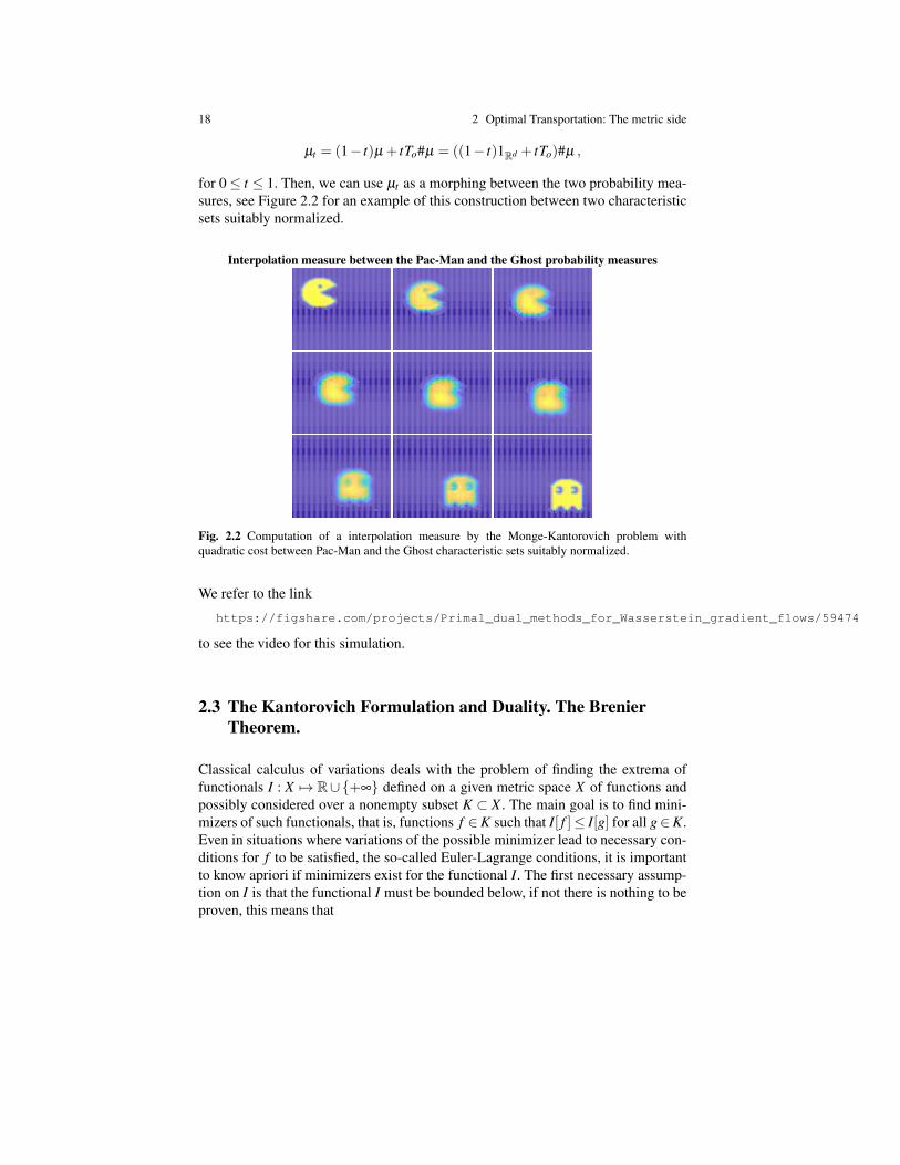
µt = (1− t)µ + tTo#µ = ((1− t)1Rd + tTo)#µ ,
for 0≤ t ≤ 1. Then, we can use µt as a morphing between the two probability mea-sures, see Figure 2.2 for an example of this construction between two characteristicsets suitably normalized.
Interpolation measure between the Pac-Man and the Ghost probability measures
Fig. 2.2 Computation of a interpolation measure by the Monge-Kantorovich problem withquadratic cost between Pac-Man and the Ghost characteristic sets suitably normalized.
We refer to the link
https://figshare.com/projects/Primal_dual_methods_for_Wasserstein_gradient_flows/59474
to see the video for this simulation.
2.3 The Kantorovich Formulation and Duality. The BrenierTheorem.
Classical calculus of variations deals with the problem of finding the extrema offunctionals I : X 7→ R∪+∞ defined on a given metric space X of functions andpossibly considered over a nonempty subset K ⊂ X . The main goal is to find mini-mizers of such functionals, that is, functions f ∈K such that I[ f ]≤ I[g] for all g∈K.Even in situations where variations of the possible minimizer lead to necessary con-ditions for f to be satisfied, the so-called Euler-Lagrange conditions, it is importantto know apriori if minimizers exist for the functional I. The first necessary assump-tion on I is that the functional I must be bounded below, if not there is nothing to beproven, this means that
2.3 The Kantorovich Formulation and Duality. The Brenier Theorem. 19
I∗ := inffI[ f ] : f ∈ K ⊂ X>−∞.
This shows the existence of a minimizing sequence, that is, a sequence fn ∈ K suchthat I[ fn]→ I∗. Notice that it is not even clear that if there is f ∈ X achieving theinfimum, then f does belong to K. The direct method of the calculus of variationsis an adapted version for general metric spaces of the classical Weierstrass criterionfor the existence of extremal points of continuous functions in compact sets in fi-nite dimensions. It can be summarized as “compactness + semi-continuity” leads toexistence of nontrivial minimization problems.
Definition 2.4. A functional I : X 7→ R∪+∞ on a metric space X is said to belower semi-continuous (l.s.c), if for every sequence fn ∈ X such that fn → f , wehave I[ f ]≤ liminfn I[ fn].
Theorem 2.2 (Direct Method of Calculus of Variations). A lower semi-continuousfunctional I : X 7→ R∪+∞ defined on a metric space X achieves its infimum inany compact subset K⊂X where I is bounded from below, that is, there exists fo ∈Ksuch that I[ fo] = minI[ f ] : f ∈ K.Proof. Since I is bounded below in K, there exists a minimizing sequence in K, thatis, a sequence fn ∈ K such that I[ fn]→ I∗ with I∗ = inf f I[ f ] : f ∈ K ⊂ X>−∞.Since K is a compact subset of X , then fn has a convergent subsequence to a limitingfunction fo ∈ K. Without loss of generality, we can assume that the minimizingsequence is convergent to fo ∈ K with I[ fo]≥ I∗ by its definition. By virtue of lowersemi-continuity we deduce that I[ fo]≤ liminfn I[ fn] = I∗, and therefore the infimumof the functional in K is achieved at fo, I∗ = I[ fo], and actually the infimum is aminimum. ut
A direct application of the previous theorem leads to the existence of optimaltransference plans.
Theorem 2.3 (Existence of optimal transference plans). Assume that the costfunction c : Rd×Rd 7→ [0,∞) is lower semi-continuous. Given two probability mea-sures µ and ν , then there exists an optimal transference plan, that is, there existsa Πo ∈ Γ (µ,ν) achieving the infimum in the Kantorovich formulation of optimaltransport
I∗ :=∫Rd×Rd
c(x,y)dΠo(x,y) = minΠ∈Γ (µ,ν)
∫Rd×Rd
c(x,y)dΠ(x,y).
Proof. Since µ and ν are probability measures, then for any ε > 0 there exists R> 0such that
µ(Rd \BR)≤ ε and ν(Rd \BR)≤ ε ,
and thus
Π((Rd×Rd)\ (BR×BR))≤Π(Rd× (Rd \BR))+Π((Rd \BR)×Rd)
= µ(Rd \BR)+ν(Rd \BR)≤ 2ε ,

20 2 Optimal Transportation: The metric side
for all Π ∈Γ (µ,ν). Hence the set of transference plans Γ (µ,ν) is tight in P(Rd×Rd). By Prokhorov’s theorem, the closure of the set of transference plans in theweak topology is compact. By definition of the convergence in the weak or narrowtopology, it is easy to check that the set of transference plans Γ (µ,ν) is closed.Therefore, we consider the functional
I[Π ] =∫Rd×Rd
c(x,y)dΠ(x,y)
defined on the compact set of all transference plans Π ∈ Γ (µ,ν), w.r.t. the weaktopology of measures. On the other hand, since c is a l.s.c. bounded from belowfunction in Rd×Rd , it can be approximated by an increasing sequence of continuousand bounded functions cn in Rd ×Rd (this statement is an exercise). Monotoneconvergence theorem implies that
In[Π ] =∫Rd×Rd
cn(x,y)dΠ(x,y) I[Π ]
for all Π ∈Γ (µ,ν). Notice that since cn is continuous and bounded, the functionalsIn are trivially continuous in the weak topology. Moreover, I[Π ] = supn In[Π ], andthus I is l.s.c in the weak topology as a supremum of continuous functionals in theweak topology (this statement is an exercise). We now have all the ingredients torepeat the same argument of the direct method of the calculus of Variations The-orem 2.2, but with the weak topology instead of the metric topology to obtain theannounced result. ut
Notice that if we use that the set of probability measures P(Rd) endowed withthe weak topology is metrizable, the previous result can be considered a direct ap-plication of Theorem 2.2.
The previous theorem gives a rough answer to the existence of optimal transfer-ence plans but much more can be obtained by realizing that the Kantorovich refor-mulation of the transportation problem is a linear optimization problem under con-vex constraints, given by linear equalities or inequalities. Therefore, this is the placein which convex analysis and duality in optimization plays an important role. Kan-torovich realized this and he introduced duality together with an economic interpre-tation of the dual variables as shadow prices. The idea is to include the constraints onthe marginals as Lagrange multipliers rewriting the minimization problem with con-straints as an inf−sup optimization problem without constraints. More precisely, letus express the constraint Π ∈ Γ (µ,ν) as follows: if Π ∈M+(Rd ×Rd), then taketwo functions ϕ,ψ ∈Cb(Rd), acting as Lagrange multipliers, to have
R =
0 if Π ∈ Γ (µ,ν)
+∞ otherwise,
with R defined by

2.3 The Kantorovich Formulation and Duality. The Brenier Theorem. 21
R := supϕ,ψ∈Cb(Rd)
∫Rd
ϕ(x)dµ(x)+∫Rd
ψ(y)dν(y)−∫Rd×Rd
(ϕ(x)+ψ(y))dΠ(x,y).
Hence, we can remove the constraint on Π if we add the quantity R to I[Π ], sinceif the constraint is satisfied we are not adding anything and if not the infinity valueswill be avoided by the minimization. Therefore the Kantorovich problem is equiva-lent to the following inf−sup problem: finding Π ∈M+(Rd×Rd) such that
infΠ
supϕ,ψ
∫Rd
ϕ(x)dµ(x)+∫Rd
ψ(y)dν(y)+∫Rd×Rd
(c(x,y)−ϕ(x)−ψ(y))dΠ(x,y).
Notice that we have also relaxed the mass constraint on Π too.Assume now that the inf and sup can be exchanged, that is, the inf−sup problem
is equivalent to the sup− inf problem. This is not always possible, the main tool infinite dimensional convex analysis is called the Rockafellar theorem. The more gen-eral Fenchel-Rockafellar duality theorem is needed in order to show this rigorously,this is outside the scope of this course, we refer to [21, 18] for further information.The exchange of infimum and supremum is true for the Kantorovich reformulationof the transportation problem under the assumption of a l.s.c. cost function c. Now,coming back to the sup− inf problem written as
supϕ,ψ
∫Rd
ϕ dµ +∫Rd
ψ dν + infΠ
(∫Rd×Rd
(c(x,y)−ϕ(x)−ψ(y))dΠ(x,y))
,
we again notice that the infimum problem can be written as a constraint on the pairof functions (ϕ,ψ) by realizing that
S =
0 if ϕ(x)+ψ(y)≤ c(x,y) on Rd×Rd
−∞ otherwise,
with
S := infΠ
(∫Rd×Rd
(c(x,y)−ϕ(x)−ψ(y))dΠ(x,y)),
(this statement is an exercise). Therefore, the sup− inf can be rewritten as an opti-mization problem with constraints:
J∗ := supϕ,ψ∈Cb(Rd)
∫Rd
ϕ dµ +∫Rd
ψ dν : ϕ(x)+ψ(y))≤ c(x,y).
This the the so-called dual optimization problem to the Kantorovich problem. It iseasy to observe that J∗ ≤ I∗ just by integrating the constraint ϕ(x)+ψ(y))≤ c(x,y)against the measure Π(x,y), and thus J∗ < +∞. In order to cope with probabilitymeasures in the whole space Rd , we need to further relax the dual optimizationproblem by considering

22 2 Optimal Transportation: The metric side
J∗ := sup(ϕ,ψ)∈Φc
J[ϕ,ψ] , with J[ϕ,ψ] :=∫Rd
ϕ dµ +∫Rd
ψ dν
and
Φc :=(ϕ,ψ) ∈ L1(dµ)×L1(dν) : ϕ(x)+ψ(y)≤ c(x,y)a.e. w.r.t. µ×ν
.
It is not difficult to check that J∗ ≤ I∗ still holds for this relaxed problem (this state-ment is an exercise). Let us now state the duality theorem in full generality whoseproof is outside the scope of this basic course, see [21, 18] for details.
Theorem 2.4. Given two probability measures µ,ν ∈P(Rd), and a lower semi-continuous cost function c : Rd×Rd 7→ [0,∞), then there is no duality gap J∗ = I∗.
Let us know focus on the particular but important case of the euclidean costfunction c(x,y) = 1
2 |x− y|2 and show the existence of maximizers to the dual opti-mization problem. We first introcuce some basic concepts of convex analysis. Givena function f : Rd 7→ R∪+∞, we say that it is proper if f is not identically +∞.Given a proper function, we define its Legendre-Fenchel transform f ∗ as
f ∗(y) = supx∈Rd
(x · y− f (x)) for all y ∈ Rd .
Notice that the Legendre-Fenchel transform of 1p |x|p is 1
q |x|q with 1p +
1q = 1, 1 <
p< ∞. Similarly, given a function ϕ : Rd 7→R∪−∞, we say that it is proper if ϕ
is not identically −∞ and its c-transform is defined as
ϕc(y) = inf
x∈Rd( 1
2 |x− y|2−ϕ(x)) for all y ∈ Rd .
We define c-concave functions as functions that are the c-transform of some func-tion.
Let us remark that since f ∗ is defined as the supremum of affine functions ony then f ∗ is a convex function. It is important to notice that the Legendre-Fencheltransform f ∗ induces a duality between l.s.c. proper convex functions. More pre-cisely, one can prove that a proper function is convex and l.s.c. if and only if thereexists g proper function with f = g∗, in which case f ∗∗ = f . It is a classical resultin convex analysis that convex functions are locally Lipschitz and a.e. differentiablein the interior of the set where they are finite. We refer to [17] as a good source ofconvex analysis results, a summary can be found in [21, Chapter 2] and [18, Section1.6].
It is easy to check by definition that for a proper function ϕ : Rd 7→ R∪−∞,then
12 |y|2−ϕ
c(y) =( 1
2 |x|2−ϕ(x))∗. (2.2)
Notice we infer that 12 |y|2−ϕc(y) is convex for a c-concave function f = ϕc. In
particular, this implies that if f is continuous and concave then f cc = f . In fact, thislast result is more general: f cc = f characterizes the set of c-concave functions, see[18].

2.3 The Kantorovich Formulation and Duality. The Brenier Theorem. 23
With these notions at hand, let us check that in order to solve the dual optimiza-tion problem, we can restrict ourselves to pairs of c-concave functions. Let us alsodenote by P2(Rd) the set of probability measures with bounded second moment,i.e.,
P2(Rd) :=
µ ∈P(Rd) :∫Rd|x|2 dµ(x)< ∞
.
Given two probability measures µ,ν ∈P(Rd), let us denote by M the quantity
M :=∫Rd|x|2 dµ(x)+
∫Rd|x|2 dν(x).
Lemma 2.1. Given two probability measures µ,ν ∈P(Rd), then for any a∈R andany (ϕ,ψ) ∈ Φc, one can change the values of (ϕ,ψ) on a zero measure set withrespect to µ×ν such that ϕ(x)+ψ(y)≤ c(x,y) for all x,y ∈ Rd . Moreover, for thenew pair, denoted the same for simplicity, we have J[ϕcc−a,ϕc +a]≥ J[ϕ,ψ] andϕcc(x)+ϕc(y)≤ c(x,y) for all x,y ∈ Rd .
Furthermore, if there exists (Cx,CY ) ∈ L1(dµ)×L1(dν) such that ϕcc ≤Cx andϕc ≤CY and J[ϕ,ψ]>−∞, then (ϕcc−a,ϕc +a) ∈Φc.
Proof. Since J[ϕcc−a,ϕc +a] = J[ϕcc,ϕc] for all a ∈R, we are reduced to show itfor a = 0. Since the value of
J[ϕ,ψ] :=∫Rd
ϕ dµ +∫Rd
ψ dν
does not change by changing the values of (ϕ,ψ) on a zero measure set with respectto µ×ν , then we can set (ϕ,ψ)= (−∞,−∞) whenever the inequality ϕ(x)+ψ(y)≤c(x,y) is not satisfied. Therefore, we can assume the inequality ϕ(x)+ψ(y)≤ c(x,y)for all x,y ∈ Rd . Let us remark that by definition of the c-transform we get
ϕc(y) = inf
x∈Rd( 1
2 |x− y|2−ϕ(x))≥ ψ(y)
since ϕ(x)+ψ(y)≤ c(x,y) for all x,y ∈ Rd , and thus ϕc(y)≥ ψ(y) for all y ∈ Rd .Similarly, one can prove that
ϕcc(x) = inf
y∈Rdsupz∈Rd
( 12 |x− y|2− 1
2 |y− z|2 +ϕ(z))≥ ϕ(x)
by choosing z = x. By definition we have
ϕcc(x)+ϕ
c(y) = infz∈Rd
( 12 |x− z|2−ϕ
c(z)+ϕc(y))≤ c(x,y),
where the last inequality holds by choosing z = y. For the furthermore part of thelemma, one only needs to show the integrability statement: (ϕcc,ϕc) ∈ L1(dµ)×L1(dν). Note that by assumption

24 2 Optimal Transportation: The metric side∫Rd(Cx−ϕ
cc)dµ +∫Rd(Cy−ϕ
c)dν ≤ M− J[ϕ,ψ]
with M given by
M =∫Rd
Cx dµ +∫Rd
Cy dν .
Since Cx−ϕcc ≥ 0 and Cy−ϕc ≥ 0, then it follows that Cx−ϕcc ∈ L1(dµ) andCy − ϕc ∈ L1(dν), and thus by the assumption (Cx,CY ) ∈ L1(dµ)× L1(dν), weobtain (ϕcc,ϕc) ∈ L1(dµ)×L1(dν) as desired. ut
We now get an upperbound on maximizing sequences.
Lemma 2.2. Given two probability measures µ,ν ∈P2(Rd), then there exists amaximizing sequence (ϕk,ψk) ∈ Φc for the dual optimization problem, that is,J[ϕk,ψk] J∗ such that ϕk(x)+ψk(y) ≤ c(x,y), ϕk(x) ≤ |x|2 and ψk(y) ≤ |y|2 forall x,y ∈ Rd and k ∈ N.
Proof. Notice that 0 = J[0,0]≤ J∗ ≤ I∗ ≤M since 12 |x−y|2 ≤ |x|2+ |y|2. Therefore,
there exists a maximizing sequence composed by proper functions (ϕk,ψk) ∈ Φc.Using the first part of Lemma 2.1, we can assume without loss of generality thatϕk(x)+ψk(y)≤ c(x,y) for all x,y ∈ Rd and all k ∈ Rd . We define the sequence
ak = infy∈Rd
(|y|2−ϕck (y)) .
Let us first show that ak ∈ R. Since (ϕk,ψk) ∈ Φc, then ϕk(x) ≤ c(x,y)−ψk(y) forall y ∈ Rd . Since ψk is a proper function, there exists bo (possibly depending on k),such that ϕk(x)≤ c(x,yo)+bo. Then
ϕck (yo) = inf
x∈Rd( 1
2 |x− yo|2−ϕk(x))≥−bo ,
and thus ak ≤ |yo|2−ϕck (yo)≤ |yo|2 +bo <+∞. Similarly, we also have
|y|2−ϕck (y)= sup
x∈Rd(|y|2− 1
2 |x−y|2+ϕk(x))≥ supx∈Rd
(−|x|2+ϕk(x))≥−|xo|2+ϕk(xo)
for any xo ∈Rd and for all y∈Rd , where again we used 12 |x−y|2 ≤ |x|2+ |y|2. Since
ϕk is proper, then we have ak ≥−|xo|2+ϕk(xo)>−∞ for some xo ∈Rd . With this athand, the new pair (ϕk, ψk) := (ϕcc
k −ak,ϕck +ak) is well defined and due to Lemma
2.1 it satisfies J[ϕk, ψk]≥ J[ϕk,ψk] and ϕk(x)+ ψk(y)≤ c(x,y)a.e. w.r.t. µ×ν .Therefore, we only need to show the integrability (ϕk, ψk) ∈ L1(dµ)×L1(dν) to
deduce that (ϕk, ψk)∈Φc by the last part of Lemma 2.1 and finish the proof. Clearlyby definition of ak, we get ψk(y) = ϕc
k (y)+ ak ≤ |y|2. By definition of ϕcck (x), we
deduce
ϕk(x)−|x|2 = infy∈Rd
( 12 |x− y|2−ϕ
ck (y)−ak−|x|2)≤ inf
y∈Rd(|y|2−ϕ
ck (y)−ak) = 0
due to 12 |x− y|2 ≤ |x|2 + |y|2 again. ut

2.3 The Kantorovich Formulation and Duality. The Brenier Theorem. 25
We finally can arrive to show the existence of maximizers for the dual optimiza-tion problem.
Theorem 2.5. Given two probability measures µ,ν ∈ P2(Rd), then there exists(ϕo,ψo) ∈Φc such that J∗ = J[ϕo,ψo], and thus
J[ϕo,ψo] = J∗ = max(ϕ,ψ)∈Φc
J[ϕ,ψ] .
Furthermore, it can be chosen such that (ϕo,ψo) = (ηcco ,η
co) with ηo ∈ L1(dµ) and
satisfying the inequalities ϕo(x)+ψo(y)≤ c(x,y), ϕo(x)≤ |x|2 and ψo(y)≤ |y|2 forall x,y ∈ Rd .
Proof. Notice again that 0 = J[0,0] ≤ J∗ ≤ I∗ ≤ M by the assumption, there-fore using Lemma 2.2 we have a maximing sequence (ϕk,ψk) ∈ Φc satisfyingJ[ϕk,ψk] J∗ such that ϕk(x)+ψk(y) ≤ c(x,y), ϕk(x) ≤ |x|2 and ψk(y) ≤ |y|2 forall x,y ∈ Rd and k ∈ N. Take l ∈ N and we define the cut-off sequence of functions(ϕ
(l)k ,ψ
(l)k ) as
ϕ(l)k (x) = maxϕk(x)−|x|2,−l+ |x|2
ψ(l)k (y) = maxψk(y)−|y|2,−l+ |y|2 .
It is easy to check that both sequences are decreasing in l ∈N converging as l→∞ atall points to the original pair (ϕk,ψk), that is, ϕk ≤ ϕ
(l+1)k ≤ ϕ
(l)k and ψk ≤ ψ
(l+1)k ≤
ψ(l)k with ϕ
(l)k → ϕk and ψ
(l)k →ψk as l→∞. Moreover,−l ≤ ϕ
(l)k (x)−|x|2 ≤ 0 and
−l ≤ ψ(l)k (y)−|y|2 ≤ 0 for all x,y ∈ Rd and k, l ∈ N. Moreover, one can also check
that
ϕ(l)k (x)+ψ
(l)k (y)≤maxϕk(x)+ψk(y)−|x|2−|y|2,−l+ |x|2 + |y|2
≤maxc(x,y)−|x|2−|y|2,−l+ |x|2 + |y|2 , (2.3)
for all x,y ∈ Rd and k, l ∈ N.For each fixed l ∈ N, the sequence ϕ
(l)k (x)− |x|2 is bounded in L∞(Rd), and
therefore bounded in Lp(dµ), 1≤ p≤∞ since the Lp(dµ)-norms are monotone in pfor a probability measure µ . Without loss of generality, we can assume the existenceof ϕ(l)(x)−|x|2 ∈ L2(dµ) such that ϕ
(l)k (x)−|x|2 ϕ(l)(x)−|x|2 weakly in L2(dµ).
Since |x|2 ∈ L1(dµ), then ϕ(l) ∈ L1(dµ), since L2(dµ)⊂ L1(dµ) and |x|2 ∈ L1(dµ).Moreover, since L∞(dµ)⊂ L2(dµ), then we can use 1 as a test function for the weakconvergence ϕ
(l)k (x)−|x|2 ϕ(l)(x)−|x|2 to get∫
Rdϕ(l)(x)dµ(x) = lim
k→∞
∫Rd
ϕ(l)k (x)dµ(x) . (2.4)
By a diagonalization argument and after extraction of subsequences, we can assumethat the above arguments apply for the same subsequence k for all l ∈ N. Since the

26 2 Optimal Transportation: The metric side
weak convergence preserves the ordering, we conclude that the limiting sequenceϕ(l) ∈ L1(dµ) satisfies ϕ(l+1) ≤ ϕ(l) ≤ |x|2 with |x|2 ∈ L1(dµ). Let us denote by ϕothe pointwise limit of the sequence ϕ(l), then the monotone convergence theoremimplies that the pointwise limits of ϕo satisfies∫
Rdϕo(x)dµ(x) = lim
l→∞
∫Rd
ϕ(l)(x)dµ(x) . (2.5)
An analogous procedure can be done with the sequence ψ(l)k (x), to define the limit-
ing function ψo.The pair (ϕo,ψo) is the our candidate maximiser. We need to show that (ϕo,ψo)∈
Φc. We first observe that
J∗ = limk→∞
J[ϕk,ψk]≤ limk→∞
J[ϕ(l)k ,ψ
(l)k ] = J[ϕ(l),ψ(l)]
since ϕk ≤ ϕ(l)k , ψk ≤ ψ
(l)k , and (2.4). Then,
J∗ ≤ liml→∞
J[ϕ(l),ψ(l)] = J[ϕo,ψo]
due to (2.5). Hence, if (ϕo,ψo) ∈ Φc then (ϕo,ψo) maximises J[ϕ,ψ] and is a so-lution to the dual optimization problem. By taking the limit k→ ∞ and then l→ ∞
in (2.3), we get ϕo(x)+ψo(y) ≤ c(x,y) for all x,y ∈ Rd . Notice here that we usethat weak limits preserve ordering. Moreover, since ϕ(l) ≤ |x|2 and ψ(l) ≤ |x|2 thenϕo(x)≤ |x|2 and ψo(y)≤ |y|2 for all x,y ∈ Rd . Finally, integrability follows from
0≤∫Rd(|x|2−ϕo(x))dµ(x)+
∫Rd(|y|2−ψo(y))dν(y)≤−J[ϕo,ψo]+M≤−J∗+M ,
where we used ϕo(x)+ψo(y) ≤ c(x,y) in the first inequality, and then since |x|2−ϕo ≥ 0 and |x|2−ψo ≥ 0, both integrals are finite and thus, |x|2−ϕo(x) ∈ L1(dµ)and |y|2−ψo(y)∈ L1(dν). Hence, ϕo(x)∈ L1(dµ) and ψo(y)∈ L1(dν) since µ,ν ∈P2(Rd) finalizing the proof of the claim (ϕo,ψo) ∈Φc. A further application of thedouble c-transform trick in Lemma 2.1 shows the additional statement in the formof the obtained maximizer (this statement is an exercise). ut
The pair of functions (ϕo,ψo) achieving the maximum are called Kantorovichpotentials for the dual optimization problem, and they can be assumed to be c-concave functions without loss of generality. In fact, given a maximizer of the dualoptimization problem (ϕo,ψo), it is not difficult to show that it is equal µ and ν-a.e.respectively to c-concave Kantorovich potentials. We now take advantage further oftheir definitions as c-transforms of a given η ∈ L1(dµ). We insisted to do all the pre-vious computations with c-concave functions to show that this proof has the poten-tial to be generalizable to a family of costs functions much larger than the quadraticcost. Let us check that the Kantorovich c-concave potentials are in fact more regularthan simply integrable functions taking advantage of its particular form.
2.3 The Kantorovich Formulation and Duality. The Brenier Theorem. 27
Corollary 2.1. Any c-concave Kantorovich potentials for the dual optimizationproblem are locally Lipschitz in the interior of the set where they are finite. Fur-thermore, the Kantorovich potentials can be chosen of the form (ϕo,ϕ
co) with ϕo
c-concave and satisfying the inequalities ϕo(x)+ϕco(y) ≤ c(x,y), ϕo(x) ≤ |x|2 and
ϕco(y)≤ |y|2 for all x,y ∈ Rd .
Proof. Since (ϕo,ψo) = (ηcco ,η
co) with ηo ∈ L1(dµ), then each Kantorovich poten-
tial is the c-transform of some ηo ∈ L1(dµ). Since 12 |y|2−ϕc(y) is convex for a
c-concave function ϕ due to (2.2), and convex functions are locally Lipschitz con-tinuous and a.e. differentiable in the interior of the set wherever they are finite, weobtain the same property for ϕ . A further application of the double c-transform trickin Lemma 2.1 shows the additional statement in the form of the obtained maximizer(this statement is an exercise) using that for c-concave functions f cc = f . ut
The previous corollary asserts that c-concave Kantorovich potentials are a.e. dif-ferentiable with respect to the Lebesgue measure in the interior of the set whereverthey are finite. In fact, from the duality Theorem 2.4 and the existence of minimiz-ers and maximizers of the primal and the dual optimization problems in Theorems2.3 and 2.5, we deduce that given Πo optimal transference plan and a ϕo concaveKantorovich potential, then
J∗ = I∗ =∫Rd×Rd
c(x,y)dΠo(x,y) =∫Rd
ϕo(x)dµ(x)+∫Rd
ϕco(y)dν(x)
=∫Rd×Rd
(ϕo(x)+ϕco(y))dΠo(x,y).
Since ϕo(x)+ϕco(y)≤ c(x,y) for all x,y ∈ Rd from Theorem 2.5 and Corollary 2.1,
then one expects ϕo(x)+ϕco(y) = c(x,y) Πo-a.e. Let us define the support of the
measure Πo as:
Definition 2.5. The support of a measure µ ∈P(Rd) is defined as the smallestclosed set in which µ is not zero, i.e.
spt(µ) :=⋂A : A is closed and µ(Rd \A) = 0
= x ∈ Rd : µ(Br)> 0 for all r > 0 .
Therefore, one can prove that ϕo(x)+ϕco(y) = c(x,y) on spt(Πo). A full proof
of this fact needs the Knott-Smith optimality criteria using that ϕo is c-concavethat we refer to [21]. Now, given (xo,yo) ∈ spt(Πo) and using the definition ofthe c-transform ϕc
o(yo), the function x 7→ ϕo(x)− c(x,yo) achieves its minimumat x = xo. Assuming the Kantorovich potential is differentiable at xo, we deducethat ∇ϕo(xo) = xo − yo. This implies that yo is uniquely determined in terms ofxo if the Kantorovich potential ϕo is differentiable at xo by yo = xo−∇ϕo(xo) for(xo,yo)∈ spt(Πo). Since ϕo ∈ L1(dµ) and J∗ ∈R, then ϕ0 is finite µ-a.e. Since con-vex functions are differentiable a.e. on the closure of set of points where they arefinite (this is a consequence of Alexandrov’s theorem, an advanced result in con-
28 2 Optimal Transportation: The metric side
vex analysis, see [22]) and if we further assume that µ ÎL , then the Kantorovichpotential is µ-a.e. differentiable.
Therefore, if the measure µ ∈P2(Rd) is absolutely continuous, then the Kan-torovich potential is µ-a.e. differentiable and its gradient is defined uniquely µ-a.e.by the relation yo = xo−∇ϕo(xo). Therefore, we have shown that any optimal trans-ference plan in the Kantorovich reformulation of the optimal transport problem withquadratic cost can be characterized as Πo = (1Rd ×T )#µ with T (x) = x−∇ϕo(x),and therefore the optimal transference plan is unique µ-a.e. since it only depends onthe values of ∇ϕo µ-a.e.
To make the last statements completely rigorous, one can use disintegration ofmeasures that in the case of probability measures Π ∈ Γ (µ,ν) reads as: given Π ∈Γ (µ,ν) and any test function ζ ∈Cb(Rd×Rd), we can find a unique µ-a.e. definedfamily of probabilty measures µx ∈P(Rd), x∈Rd , supported inside x×Rd suchthat ∫
Rd×Rdζ (x,y)dΠ(x,y) =
∫Rd
∫Rd
ζ (x,y)dµx(y)dµ(x).
This is also the precise definition of conditional law in probability theory. If X is arandom variable with law µ and Y is a random variable with law ν , Π ∈ Γ (µ,ν)represents the law of a coupling (X ,Y ) between X and Y . Then, µx represents the lawof the conditional probability of the random variable Y subject to knowing X = x.With the disintegration of measures at hand, see [3] for a proof, we have previouslyshown that by disintegrating the measure Πo with respect to µ then µx = δy=T (x)since T (x) is the only point on the support of Πo for x µ-a.e. The above consider-ations can now be stated as the following result which is due to Yann Brenier in amore general form.
Theorem 2.6. [Monge finally meets Kantorovich] Given two probability measuresµ,ν ∈P2(Rd) with µ ÎL , then there exists an unique optimal transference planfor the quadratic cost of the form Πo = (1Rd ×T )#µ ∈ Γ (µ,ν) achieving the infi-mum in the Kantorovich formulation of optimal transport∫
Rd|x−T (x))|2 dµ(x) = min
Π∈Γ (µ,ν)
∫Rd×Rd
|x− y|2 dΠ(x,y).
Moreover, this map is given by T (x) = x−∇ϕo(x) defined uniquely µ-a.e. whereϕo(x) is a c-concave Kantorovich potential.
The previous theorem finally connects the Monge transportation problem to theKantorovich reformulation by showing the the infimum on the Monge problem isachieved and coincides with the minimum of the Kantorovich reformulation forthe quadratic cost if µ Î L . Notice also that the optimal transport map can bechosen as T = ∇Ψ with Ψ a convex function by taking Ψ = 1
2 |x|2−ϕo(x). Theuniqueness part is not proven here and we refer to the literature. All the resultspresented for the quadratic cost can be similarly generalized to costs functions of theform c(x,y) = h(x− y) with h strictly convex. For instance, h(s) = |s|p, 1 < p < ∞.We refer to [21, 22, 18].

2.4 Transport distances between measures: properties. 29
2.4 Transport distances between measures: properties.
The goal of this section is to introduce transport distances based on the optimaltransport introduced in the previous section. Let us take simple cases first. Assumethat µ,ν ∈P2(Rd) are just two Dirac Deltas at two different points µ = δxo andν = δx1 with xo,x1 ∈Rd and xo 6= x1. Then, it is easy to see that the norm introducedin the set of finite signed measures is ‖δxo − δx1‖ = 2 no matter how close the twopoints are. Notice that in fact the norm introduced in Definition 2.1 is just the totalvariation norm between measures. It is clearly not a good distance if we think abouthow close or how far are δxo , δx1 in terms of the distance between the points wherethey are concentrated on. Now, let us take any Π ∈ Γ (δxo ,δx1). It is clear that theonly possible transference plan is the product measure δxo ×δx1 , for instance usingthe disintegration of measures theorem. Therefore, any map that sends xo onto x1is an optimal map for the optimal mass transportation problem for any l.s.c. costfunction c(x,y) and therefore the optimal cost is c(x0,x1). A desirable property ofthe cost function satisfied by all the basic costs c(x,y) = |x− y|p, 1 ≤ p < ∞, isthat the cost is continuous and has zero value for x = y. Thus we could considerthe value of the cost transporting δxo onto δx1 as a measure of the distance betweenthe probability measures δxo and δx1 . Moreover, it is a measure that is continuous asxo→ x1. These ideas lead to the following definition.
Definition 2.6. The Wasserstein distance between µ and ν , dp, 1 ≤ p < ∞ can bedefined by
dpp(µ,ν) = inf
Π∈Γ (µ,ν)
∫Rd×Rd
|x− y|p dΠ(x,y),
i.e., by the p-th root of the value of the optimum in the Kantorovich reformulationof the mass transport problem with cost c(x,y) = |x− y|p, 1≤ p< ∞.
Notice that the Wasserstein distance dp is finite for any measures µ,ν ∈Pp(Rd),being
Pp(Rd) :=
µ ∈P(Rd) :∫Rd|x|p dµ(x)< ∞
,
1 ≤ p < ∞. The classical Monge-Kantorovich problem was posed for the case ofthe Euclidean distance, p = 1, and it is usually refered as the Monge-Kantorovichdistance. Another name in the engineering and applied mathematical sciences usedis the earth movers distance alluding to the origin of the Monge problem. The nameWasserstein was used due to classical papers popularizing the use of d2 in PartialDifferential Equations, and it has kept that name for the last 20+ years. However,historically attributing to Wasserstein the name of this distance is not wrong butnot completely fair either. Many people call the distances dp as transport distancestoo. More information about other appearances in the literature of these transportdistances can be read in the summer school notes in [11].
From a probabilistic point of view, the Wasserstein distance dp can be alterna-tively defined as
30 2 Optimal Transportation: The metric side
dpp(µ,ν) = inf
(X ,Y )∈Γ
E [|X−Y |p] , (2.6)
where Γ is the set of all possible couplings of random variables (X ,Y ) with laws µ
and ν respectively, i.e., X ,Y : (S ,A ,P) −→ L measurable maps from a prob-ability space of reference (S ,A ,P) onto the Lebesgue space L and (X ,Y ) :(S ,A ,P) −→ L ×L such that the laws or image measures are X#P = µ ,Y #P = ν , and (X ,Y )#P = Π with Π ∈ Γ (µ,ν).
In order to prove the triangle inequality, we need some preliminary results.
Lemma 2.3. [Gluing lemma] Given probability measures µ,ν ,ω ∈P(Rd), Π1 ∈Γ (µ,ν) and Π2 ∈Γ (ν ,ω), there exists a measure γ ∈P(R3d) such that P12#γ =Π1and P23#γ = Π2 being P12 and P23 the projections maps into the first and the lasttwo variables respectively, i.e., P12(x,y,z) = (x,y) and P23(x,y,z) = (y,z) for allx,y,z ∈ Rd .
Proof. By the disintegration of measures, we can write
Π1(A×B) =∫
Bν
1y (A)dν(y) and Π2(B×C) =
∫B
ν2y (C)dν(y)
for some family of probability measures ν iy, i1,2, and any Borel sets A,B,C in Rd .
We define γ ∈P(R3d) given by
γ(A×B×C) =∫
Bν
1y (A)ν
2y (C)dν(y) .
It is easy to check that γ(A×B×Rd) = Π1(A×B) and γ(Rd×B×C) = Π2(B×C)as desired.
Proposition 2.1. The distance dp is a metric on Pp(Rd).
Proof. Since the cost c(x,y) = |x− y|p is nonnegative and symetric, it is easy tosee that the optimal value is nonnegative and that the distance is symmetric on itsarguments dp
p(µ,ν) = dpp(ν ,µ). For the last statement, notice that Π ∈ Γ (µ,ν) if
and only if S#Π ∈ Γ (ν ,µ) with S : Rd ×Rd 7→ Rd ×Rd given by S(x,y) = (y,x).Now, if µ = ν , we can take Π(x,y) = δx(y)µ(x) ∈ Γ (µ,ν) to obtain that
0≤ dpp(µ,µ)≤
∫Rd×Rd
|x− y|p dΠ(x,y) = 0
since x = y Π -a.e. Now, if dpp(µ,µ) = 0 then there exists Π(x,y) ∈ Γ (µ,ν) such
that x = y Π -a.e. Hence, for any test function ζ ∈Cb(Rd), we have∫Rd
ζ (x)dµ(x) =∫Rd×Rd
ζ (x)dΠ(x,y) =∫Rd×Rd
ζ (y)dΠ(x,y) =∫Rd
ζ (y)dν(y) ,
and thus µ = ν by the Riesz representation theorem. The only remaining propertyto show is the triangular inequality. Let µ,ν ,ω ∈P(Rd), Π1 ∈ Γ (µ,ν) and Π2 ∈
2.4 Transport distances between measures: properties. 31
Γ (ν ,ω) optimal transference plans by Theorem 2.3. Lemma 2.3 implies there existsa measure γ ∈P(R3d) such that P12#γ =Π1 and P23#γ =Π2. We define Π3 =P13#γ
being P13(x,y,z) = (x,z) for all x,y,z ∈ Rd . One can check that Π3 ∈ Γ (µ,ω) (thisstatement is an exercise). Using the definition of the distance dp, the definition of γ ,the triangle inequality, the Minkowski inequality for Lp spaces, and the optimalityof Π1 and Π2, we obtain
dp(µ,ω)≤(∫
Rd×Rd|x− z|p dΠ3(x,y)
) 1p
=
(∫Rd×Rd×Rd
|x− z|p dγ(x,y,z)) 1
p
≤(∫
Rd×Rd×Rd(|x− y|+ |y− z|)p dγ(x,y,z)
) 1p
≤(∫
Rd×Rd×Rd|x− y|p dγ(x,y,z)
) 1p
+
(∫Rd×Rd×Rd
|y− z|p dγ(x,y,z)) 1
p
=
(∫Rd×Rd
|x− y|p dΠ1(x,y)) 1
p
+
(∫Rd×Rd
|y− z|p dΠ2(y,z)) 1
p
= dp(µ,ν)+dp(ν ,ω) ,
as desired. ut
Finally, let us remark that the sequence of metrics dp(µ,ν) is nondecreasing inp, 1≤ p<∞. This is a simple consequence of the Holder’s inequality for Lp-spaces.This allows to define a quantity that we call the ∞-Wasserstein distance as
d∞(µ,ν) := limp∞
dp(µ,ν).
This is at least a metric on the set of compactly supported probability measures. Wewill not discuss much more on this interesting transport distance and refer to theliterature for more details. By the monotone property of the distances dp, we deducethat for compactly supported probability measures, the topology induced by dp getsfiner as p increases.
Notice also that if µ,ν ∈P(Rd) are both supported on a ball BR then
dp(µ,ν)≤ (2R)(p−1)/pd1(µ,ν)1/p . (2.7)
This is due to the fact that for any Π ∈Γ (µ,ν) we have Π(Rd×(Rd \BR))= ν(Rd \BR) = 0 and Π((Rd \ BR)×Rd) = µ(Rd \ BR) = 0. Thus, we deduce Π((Rd×Rd)\(BR×BR))= 0, and therefore, spt(Π)⊂ BR×BR. Take now the optimal transferenceplan Πo ∈ Γ (µ,ν) for the distance d1, then
dpp(µ,ν)≤
∫Rd×Rd
|x− y|p dΠo(x,y) =∫
BR×BR
|x− y|p dΠo(x,y)
≤ (2R)(p−1)∫
BR×BR
|x− y|dΠo(x,y) = (2R)(p−1)d1(µ,ν) ,

32 2 Optimal Transportation: The metric side
leading to the desired inequality.Let us focus now in understading the notion of convergence in transport metrics
dp. We will denote by Lip(Rd) the set of Lipschitz functions on Rd and by W 1,∞(Rd)the set of bounded and Lipschitz functions on Rd .
Corollary 2.2 (Convergence of averages with dp). Given probability measuresµ,ν ∈Pp(Rd) and ϕ ∈ Lip(Rd) with Lipschitz constant L, then we have∣∣∣∣∫Rd
ϕ(x)dµ(x)−∫Rd
ϕ(x)dν(x)∣∣∣∣≤ Ldp(µ,ν).
Proof. Since dp(µ,ν) is nondecreasing in p, we can reduce to show the statementfor d1. Let Πo(x,y) an optimal plan between µ,ν ∈P1 for d1. Then∫
Rd×Rd|x− y|dΠo(x,y) = d1(µ,ν),
and we can write∫Rd
ϕ(x)dµ(x)−∫Rd
ϕ(x)dν(x) =∫Rd×Rd
(ϕ(x)−ϕ(y))dΠo(x,y).
Using that ϕ is Lipschitz with constant L and estimating, we get∣∣∣∣∫Rdϕ(x)dµ(x)−
∫Rd
ϕ(x)dν(x)∣∣∣∣≤ ∫Rd×Rd
|ϕ(x)−ϕ(y)|dΠo(x,y)
≤ L∫Rd×Rd
|x− y|dΠo(x,y)≤ Ld1(µ,ν)
giving the assertion. ut
In the noticeable case of the Monge-Kantorovich distance d1, the previous corol-lary is a characterization by duality. More precisely, as a consequence of Fenchel-Rockafellar’s duality principle, one can deduce the Kantorovich-Rubinstein theorem[21, Theorem 1.14] giving that
d1(µ,ν)=sup∣∣∣∣∫Rd
ϕ(x)d(µ−ν)(x)∣∣∣∣,ϕ ∈ Lip(Rd),‖ϕ‖Lip(Rd) ≤ 1
. (2.8)
Another classical distance between measures , not necessarily probabilty measures,is the so-called Bounded Lipschitz (BL) distance, that is defined as
‖µ−ν‖BL=sup∣∣∣∣∫Rd
ϕ(x)d(µ−ν)(x)∣∣∣∣,ϕ ∈W 1,∞(Rd),‖ϕ‖W 1,∞(Rd) ≤ 1
,
that is, the dual W 1,∞(Rd)-norm. The convergence in BL-distance is equivalent toweak convergence of measures by the Pormanteau theorem. We will see next thatthe topology in d1 is finer than the topology induced by the BL-distance in Rd .
2.4 Transport distances between measures: properties. 33
However, we start by showing that on compact sets of Rd the convergence in anytransport distance is also equivalent to weak convergence of measures.
Proposition 2.2. Given a sequence of probability measures µn ∈Pp(Rd) and µ ∈Pp(Rd) supported on some euclidean ball BR. Then dp(µn,µ)→ 0 if and only ifµn converges weakly to µ .
Proof. We first notice that due to (2.7) and that d1(µn,µ) ≤ dp(µn,µ), we are re-duced to show the result for d1. The charaterization (2.8) implies directly that ifd1(µn,µ)→ 0 then µn converges weakly to µ . Here, we can use the Pormanteautheorem, a result that can be seen in basic courses of probability, or an argumentby density to go from Lipschitz to bounded continuous functions. Conversely, let ustake the subsequence µnk such that
limsupn→∞
d1(µn,µ) = limk→∞
d1(µnk ,µ) .
By the characterization (2.8), we have the existence of a sequence of 1-Lispschitzfunctions ϕk such that
d1(µnk ,µ)≤∫Rd
ϕk(x)d(µnk−µ)(x)+1k=∫
BR
(ϕk(x)−ϕk(0))d(µnk−µ)(x)+1k,
since µn ∈Pp(Rd) and µ ∈Pp(Rd) supported on BR. The sequence of functionsϕk(x) := ϕk(x)− ϕk(0) is now 1-Lipschitz and bounded defined on BR, then byAscolı-Arzela theorem, there exists a further subsequence, that we denote with thesame index, converging uniformly to a 1-Lispchitz function ϕ . Hence, we concludethat
limsupn→∞
d1(µn,µ)≤ limsupk→∞
∫BR
ϕk(x)d(µnk −µ)(x)
≤ limsupk→∞
∫BR
(ϕk(x)− ϕ(x))dµnk(x)+ limsupk→∞
∫BR
ϕ(x)d(µnk −µ)(x)
− limsupk→∞
∫BR
(ϕk(x)− ϕ(x))dµ(x)
≤ 2limsupk→∞
‖ϕk(x)−ϕ(x)‖L∞(BR)+ limsup
k→∞
∫BR
ϕ(x)d(µnk −µ)(x) = 0 ,
where we used in the last line the weak convergence of µn towards µ , and thusd1(µn,µ)→ 0 as n→ ∞. ut
Now, we come back to the whole space to study the notion of dp convergence.
Theorem 2.7. Given a sequence of probability measures µn ∈Pp(Rd) and µ ∈Pp(Rd). Then dp(µn,µ)→ 0 if and only if µn converges weakly to µ and∫
Rd|x|p dµn(x)→
∫Rd|x|p dµ(x) as n→ ∞.
34 2 Optimal Transportation: The metric side
Proof. The necessary implication is a consequence of Corollary 2.2 together withthe triangle inequality. In fact, observing that∫
Rd|x|p dµn(x) = dp
p(µn,δ0) and∫Rd|x|p dµ(x) = dp
p(µ,δ0) ,
we get by the triangle inequality for dp that
|dp(µn,δ0)−dp(µ,δ0)| ≤ dp(µn,µ)→ 0
as n→ ∞.Conversely, let us truncate the p-th moment by defining φR(x) = min(|x|,R)p
which is continuous and bounded. Therefore, by weak convergence of the sequenceµn towards µ and the convergence of the p-th moments, we get∫
Rd(|x|p−φR(x))dµn(x)→
∫Rd(|x|p−φR(x))dµ(x) as n→ ∞.
Now, we can take R large enough such that∫Rd(|x|p−φR(x))dµ(x) =
∫|x|>R
(|x|p−Rp)dµ(x)≤∫|x|>R|x|p dµ(x)≤ ε
2,
for a given fixed ε > 0, since µ ∈Pp(Rd). Therefore, for n large enough, we alsohave ∫
Rd(|x|p−φR(x))dµn(x)≤ ε .
For 0 < b < a and p ≥ 1, it is easy to check that ap + bp ≤ (a+ b)p. We can inferthat for |x|> R then (|x|−R)p ≤ |x|p−Rp = |x|p−φR(x). So for n large enough∫
|x|>R(|x|−R)p dµn(x)≤ ε and
∫|x|>R
(|x|−R)p dµ(x)≤ ε .
Let us consider the euclidean projection onto the ball BR denoted by PR, this mapis continuous, leaves invariant BR and otherwise |x−PR(x)| = |x| −R. Hence, wededuce that
dpp(µ,PR#µ)≤
∫Rd|x−PR(x)|p dµ(x) =
∫|x|>R
(|x|−R)p dµ(x)≤ ε ,
and analogously dpp(µn,PR#µn) ≤ ε . Since µn µ weakly, it is easy to check that
PR#µn PR#µ weakly, and thus using the characterization of the convergence formeasures supported in BR in Proposition 2.2, we get dp(PR#µn,PR#µ)→ 0 as n→∞.We conclude by estimating using the triangle inequality as follows:
dp(µn,µ)≤ dp(µn,PR#µn)+dp(PR#µn,PR#µ)+dp(µ,PR#µ)
≤ 2ε1/p +dp(PR#µn,PR#µ) ,
2.4 Transport distances between measures: properties. 35
for n large enough. Taking the limit n→ ∞, we get
limsupn→∞
dp(µn,µ)≤ 2ε1/p
and then, taking the limit ε → 0, we finally obtain dp(µn,µ) → 0 as n → ∞ asdesired. ut
We end this section by making a summary of the main properties of the dp dis-tances.
Proposition 2.3 (dp-properties). The space (Pp(Rd),dp) is a complete metricspace, 1≤ p< ∞. Moreover, the following properties of the distance dp hold:
i) Optimal transference plan: The infimum in the definition of the distance dp isachieved at a joint probability measure Πo called an optimal transference plansatisfying:
dpp(µ,ν) =
∫∫Rd×Rd
|x− y|2 dΠo(x,y).
ii) Convergence of measures: Given µn and µ in Pp(Rd), 1≤ p<∞, the followingassertions are equivalent:
a) dp(µn,µ) tends to 0 as n goes to infinity.b) µn tends to µ weakly and∫
Rd|x|p dµn(x)→
∫Rd|x|p dµ(x) as n→+∞.
iii) Lower semicontinuity: dp is weakly-* lower semicontinuous in each argument,1≤ p< ∞.
iv) Moments as distances: If µ ∈Pp(Rd), then
dpp(µ,δa) =
∫Rd|x|2 dµ(x).
v) Convexity: Given f1, f2, g1 and g2 in Pp(Rd) and α in [0,1], then
dpp(α f1 +(1−α) f2,αg1 +(1−α)g2)≤ αdp
p( f1,g1)+(1−α)dpp( f2,g2).
As a simple consequence, given f ,g and h in Pp(Rd), then
dp(h∗ f ,h∗g)≤ dp( f ,g)
where ∗ stands for the convolution of measures in Rd .vi) Additivity with respect to convolution of d2: Given f1, f2, g1 and g2 in P2(Rd)
with equal mean values, then
d22( f1 ∗ f2,g1 ∗g2)≤ d2
2( f1,g1)+d22( f2,g2).
36 2 Optimal Transportation: The metric side
Proof. Most of the properties have been shown except Property iii) and the last two.Properties iii) and v) are left to the reader (these statements are exercises). Noticehere that the convolution between measures is defined as usual by duality on testfunctions, meaning f ∗g for f ,g ∈P(Rd) is defined as the measure f ∗g ∈P(Rd)such that∫
Rdζ (x)d( f ∗g)(x) =
∫Rd
∫Rd
ζ (x+ y)d f (x)dg(y) ∀ζ ∈ Cb(Rd) .
Property vi) is a direct consequence of the definition of d2 in terms of random vari-ables. Let (X1,Y1), (X2,Y2) be two independent pairs of random variables, and let fi(resp. gi) be the laws of Xi (resp. Yi) i = 1,2. Suppose moreover that Xi and Yi havethe same mean value, namely E[Xi] = E[Yi] i = 1,2. If the pairs (X1,Y1), (X2,Y2)realize the optimal transference plans, then for i = 1,2
d22( fi,gi) = E
[|Xi−Yi|2
].
Notice that the law of the random variable X1 +X2 is given by f1 ∗ f2 since X1 andX2 are independent (this statement is an exercise), then
d22( f1 ∗ f2,g1 ∗g2)≤ E
[|(X1 +X2)− (Y1 +Y2)|2
]= E
[|X1−Y1|2
]+E
[|X2−Y2|2
]+2E [(X1−Y1) · (X2−Y2)]
= d22( f1,g1)+d2
2( f2,g2)
In fact, the term E [(X1−Y1) · (X2−Y2)] is equal to zero due to the independence ofthe pairs, and to the equality of the mean values. ut
2.5 One-dimensional Wasserstein metric
Given a probability measure in one dimension, µ ∈P(R), we define as usual itsdistribution function F : R 7→ [0,1] as
F(x) =∫ x
−∞
dµ(x) = µ((−∞,x]) .
Notice that the definite integral is just a notation here made precise by the secondequality. With this definition, F is a monotone nondecreasing right-continuous func-tion with F(−∞) = 0 and F(+∞) = 1, in fact it is a cadlag function. In principle, Fdoes not have an inverse since it can have plateaus, but we can define its generalizedinverse or pseudo-inverse function X : [0,1] 7→ R∪±∞ as follows:
X(η) = infx∈Rx ∈ R : F(x)≥ η
2.5 One-dimensional Wasserstein metric 37
for all η ∈ [0,1]. The infimum is a minimum as soon as the set is not empty (oth-erwise is +∞) and bounded from below (otherwise it is −∞), thanks to the rightcontinuity of F . Note that X(η)≤ x ⇐⇒ η ≤ F(x) or equivalently X(η)> x ⇐⇒η > F(x). By definition X(η) is a nondecreasing function and F(X(η)) ≥ η andX(F(x)) ≤ x. If F is increasing and continuous then F(X(η)) = η . We remind thereader some basic properties about monotone funcitions that we will use below. Amonotone function can have only a countable number of discontinuities and they arejump discontinuities if they exist. Moreover, the set of possible discontinuities haszero Lebesgue measure. In our case, this implies that both F and X have a countablenumber of jump discontinuities and plateaus, note that a plateau for F is a jumpdiscontinuity for X and viceversa, and both sets are of zero Lebesgue measure.
Proposition 2.4. Given µ ∈ P(R), and X the pseudo-inverse of its distributionfunction F, then X#L = µ . Moreover, given µ,ν ∈P(R), and X and Y their cor-responding pseudo-inverses with distribution functions F and G, then the measureγm := (X,Y)#L belongs to the admissible set Γ (µ,ν) and γm((−∞,a]×(−∞,b]) =min(F(a),G(b)). Furthermore, if µ ∈P(R) is atomless, then F#µ = L , and as aconsequence, for every l ∈ [0,1], the set x ∈ R : F(x) = l is µ-negligible.
Proof. Let us clarify that by L we mean the Lebesgue measure on the interval ofdefinition of the pseudo-inverses [0,1]. We first realize that
L (η ∈ [0,1] : X(η)≤ x) = L (η ∈ [0,1] : η ≤ F(x)) = F(x) ,
which implies that X#L and µ coincide by definition on the intervals (−∞,x] for allx ∈R. Then the two measures X#L = µ , since this family of intervals generate thewhole Borel σ -algebra on the real line. We proceed similarly to prove the secondone by computing
γm((−∞,a]× (−∞,b]) = L (η ∈ [0,1] : X(η)≤ a and Y(η)≤ b)= L (η ∈ [0,1] : η ≤ F(a) and η ≤ G(b))= min(F(a),G(b)) .
Since µ is atomless then F is a continuous function. Hence, for all a ∈ (0,1) the setF−1((−∞,a]) = (−∞,xa] with F(xa)= a. Hence, µ(F−1([0,a])) =F(xa)= a givingthe first part of the last statement. The second part is by contradiction, otherwise ifone of these sets of the form x ∈ R : F(x) = l has µ positive measure, then thiswill mean that the Lebesgue measure should have an atom at l by the first part ofthe last statement.
The mass transference plan γm is called the monotone mass transference plan.
Proposition 2.5. Given µ,ν ∈P(R). Assume that µ ∈P(R) is atomless, and Xand Y their corresponding pseudo-inverses with distribution functions F and G,then there exists a unique µ-a.e. defined nondecreasing map Tm : R 7→ R such thatν = Tm#µ given by Tm = YF.

38 2 Optimal Transportation: The metric side
Proof. Notice that the map Tm = Y F is well defined with values on R as soonas F(x) ∈ (0,1). Since the sets x ∈ R : F(x) = 0 and x ∈ R : F(x) = 1 are µ-negligible, then Tm = YF is well defined µ-a.e. The fact that Tm is nondecreasingis obvious by composition of nondecreasing function. Using Proposition 2.4, wehave that Y#L = ν and F#µ = L since µ is atomless, and thus ν = Tm#µ by thedefinition of push-forward.
Let us know prove the uniqueness part. Consider any monotone nondecreas-ing map T such that ν = T #µ . From the monotonicity, we deduce that (−∞,x] ⊂T−1((−∞,T (x)]). Thus, we have
F(x) = µ((−∞,x])≤ µ(T−1((−∞,T (x)])) = ν((−∞,T (x)]) = G(T (x)) ,
and thus by definition of pseudo-inverse T (x)≥ Y(F(x)). Assume that the inequal-ity is strict now, there there exists εo > 0 such that G(T (x)− ε) ≥ F(x) for everyε ∈ (0,εo). By monotonicity again, we have T−1((−∞,T (x)− ε]) ⊂ (−∞,x] andthen, G(T (x)−ε)≤ F(x). Thus, we get that G(T (x)−ε) = F(x) for all ε ∈ (0,εo).Then F(x) is the value that G(x) takes on an interval that is constant. We know thatthe set of plateaus on G is countable, so then it is the set of possible values that Ftakes on those intervals. The last statement in Proposition 2.4 says that each of thesesets is negligible µ-a.e. and thus it is the case for a countable union of them. There-fore the set of points x such that T (x) > Y(F(x)) is µ negligible, and thus T = Tmµ-a.e. ut
The first main result of this section characterizes the monotone plan and mapbetween two one dimensional probability measures.
Proposition 2.6. Let γ ∈ Γ (µ,ν) be a transport plan between the probability mea-sures µ,ν ∈P(R). Assume that it satisfies the property
(x,y),(x′,y′) ∈ spt(γ) and x< x′ =⇒ y≤ y′ ,
then γ = γm. In particular, there is a unique γ satisfying the previous property.
Proof. We just need to prove that
γ((−∞,a]× (−∞,b]) = min(F(a),G(b))
according to Proposition 2.4. Consider the sets A = (−∞,a]× (b,+∞) and B =(a,+∞)× (−∞,b]. By assumption it is not possible to have both γ(A) > 0 andγ(B)> 0, otherwise we contradict the assumption. Since these two sets have emptyintersection with (−∞,a]× (−∞,b] and at least, one of them has zero γ measure,then
γ((−∞,a]× (−∞,b]) = min(γ((−∞,a]× (−∞,b]∪A),γ((−∞,a]× (−∞,b]∪B)).
It is easy to see that γ((−∞,a]×(−∞,b]∪A)= γ((−∞,a]×R)=F(a). Analogouslyfor γ((−∞,a]× (−∞,b]∪B) = G(b), obtaining the desired result. ut

2.5 One-dimensional Wasserstein metric 39
The previous result allows to find the solution to the transportation problem inone dimension and leads to a more general concept that characterizes optimal trans-port in higher dimensions, the concept of cyclical monotone sets. We just finish thissection by stating the theorem without a proof that we refer to [21, 18].
Theorem 2.8. Given two probability measures µ,ν ∈ P(R), h : R 7→ [0,∞) astrictly convex function, and the cost function of the form c(x,y) = h(x−y). Assumethat the Kantorovich problem associate to the cost c among these two measures isfinite, i.e.
I∗ := minΠ∈Γ (µ,ν)
∫R×R
c(x,y)dΠ(x,y)<+∞ .
Then the infimum is achieved uniquely by γm. If µ ∈P(R) is atomless, this optimalplan is induced by the map Tm. Moreover, if we assume plain convexity for h thenγm is an optimal transport plan but the uniqueness is not guaranteed. Finally, in allcases the optimal cost can be expressed as
I∗ =∫ 1
0h(X(η)−Y(η))dη ,
where X and Y are the pseudoinverses of µ,ν ∈P(R).
Note that the previous theorem implies that the Wasserstein distance dp, 1≤ p≤∞, between two one dimensional probability measures is given by the Lp-norm ofthe difference of their corresponding pseudoinverses functions. In particular, for theMonge-Kantorovich distance, we have
d1(µ,ν) =∫ 1
0|X(η)−Y(η)|dη =
∫R|F(x)−G(x)|dx ,
(this last equality is an exercise).Finally, let us see how to connect again to some of the PDE models we saw in
the first chapter. Consider the one dimensional PDE
∂ρ
∂ t=
∂
∂x
(ρV ′), (2.9)
with V a C2 confinement potential such that V is uniformly convex, V ′(x)≥ λ > 0,with global minimum at zero. Let us consider smooth positive probability measuresolutions of (2.9), and let us denote by F(t,x) the distribution function associatedto the solution ρ(t,x) of (2.9), and X(t,η) its pseudo inverse. By the definition ofpseudo-inverse function we have
F(t,X(t,η)) = η . (2.10)
Differentiating (2.10) with respect to η gives
∂F∂x
∣∣∣x=X
∂X∂η
= 1, (2.11)

40 2 Optimal Transportation: The metric side
and twice gives∂ρ
∂x
∣∣∣x=X
(∂X∂η
)2+ρ(t,X)
∂ 2X∂η2 = 1. (2.12)
Differentiating (2.10) with respect to t gives
∂F∂ t
∣∣∣x=X
+∂F∂x
∣∣∣x=X
∂X∂ t
= 0 (2.13)
Then we collect from (2.11)-(2.12) that
∂F∂ t
∣∣∣x=X
=∫ X
−∞
∂ρ
∂ t(t,x)dx =
∫ X
−∞
∂
∂x
(ρV ′)
dx =[ρ(t,x)V ′(x)
]x=X =V ′(X)ρ(t,X) ,
which, in light of (2.13), leads us to the following evolution problem
Xt =−V ′(X), η ∈ (0,1), t > 0, (2.14)
Therefore, we can deduce that if ρ1 and ρ2 are two such solutions of (2.9) and iftheir corresponding pseudoinverses are X1 and X2, then
12
ddt
∫ 1
0(X1(t,η)−X2(t,η))2 dη =
−∫ 1
0(X1(t,η)−X2(t,η))(V ′(X1(t,η))−V ′(X2(t,η)))dη .
If the confinement potential V is uniformly convex, then V ′′(x) ≥ λ > 0 and usingTheorem 2.8, we get
ddt
d22(ρ1(t),ρ2(t))≤−2λd2
2(ρ1(t),ρ2(t)) ,
for all t ≥ 0. Gronwall’s lemma implies that
d22(ρ1(t),ρ2(t))≤ e−2λ td2
2(ρ1(0),ρ2(0)).
Therefore, for a uniformly convex confinement potential, the flow of the PDE (2.9)is a contraction in the d2 metric. Let us finally point out that X = 0 is a solutionof (2.14) that corresponds to a Dirac Delta at the minimum of the potential V inoriginal variables. In fact, one can show that δ0 is a stationary solution to (2.9) (thisstatement is left as a simple exercise). Therefore, by taking the stationary solutionδ0 as one of the solutions, then d2
2(ρ(t),δ0) ≤ e−2λ td22(ρ(0),δ0) for all solutions
of (2.9). So, solutions of (2.9) concentrate in infinite time to the Delta Dirac at theorigin. We again see that the convexity of the potential is essential to discuss thelong time asymptotics of (2.9).
We leave as an exercise to compute the equation satisfied by the pseudoinverseof the solutions of the linear Fokker-Planck equation (1.12) in one dimension and todraw conclusions about the asymptotic behavior.

2.5 One-dimensional Wasserstein metric 41
We finish this section by pointing out that this approach can be turned into aneffective numerical method to compute solutions of PDEs in one dimension of thegeneral form (1.1). We showcase this in Figures 2.3 and 2.4, where we show theevolution of the pseudoinverse function associated to the solution of the PKS model(1.22) in one dimension in sub- and supercritical cases. We see how the numericalmethod is able to capture the diffusion of the solution in the subcritical case and theconcentration in the supercritical case leading to a Dirac Delta forming in finite timeaccording to the numerical simulations.
corresponding to a compact supported density n0, we numerically solve the PKSequation on the time interval [0, 400] with χ = π. Figures 4.1 and 4.2 show theevolution of the solution both for the density (Fig. 4.2) and its inverse distributionfunction (Fig. 4.1).
0
0.5
1
0
500
1000−100
0
100
t
Figure 4.1. Inverse cumulative distri-bution function for χ = π. Note that theinitial data seems to be flat relatively to thevery large scale on the V−axis, as opposedto Figure 4.5.
−500
50
0
500
1000
0.2
0.4
xt
Figure 4.2. Cell density n as timeevolves, obtained from its inverse cumu-lative distribution function. Accordinglyto Figure 4.1, the space scale is alsovery large, and therefore the density seemshighly concentrated at t = 0.
Observe in Figure 4.1 that the branches of the inverse cumulative function Vgoes eventually to ±∞. This is expected because the support of the cell densityspreads as time goes on, and therefore the distribution tails are wider. Remind thatin the sub-critical regime, the diffusion process dominates. The scheme captureswell the collapse down to zero of the cell density and the spreading of the solution.Interestingly, this scheme handles easily with moving density’s support (note thatfinite speed of propagation is a numerical artifact) whereas the reference domain [0, 1]is fixed because we deal with probability densities (mass is conserved).
100
102
10−2
10−1
100
log(t)
log(
||n||)
Figure 4.3. L2-norm’s evolution forthe cell density n, in a log− log scale. Thedecay appears to be polynomial.
0 200 400 600 800 1000−5
−4
−3
−2
−1
t
S[n
]
Figure 4.4. Evolution of the entropyS [n] showing slow decay.
Moreover, the spreading towards zero seems to be polynomial from Figure 4.3showing the evolution of the L2-norm of the cell density in log-log scale. The entropydecay is plotted in Figure 4.4.
20
Fig. 2.3 Solution of the equation for the pseudoinverse associated to the PKS (1.22) in one dimen-sion in a subcritical case.
00.5
1
00.10.20.3−4
−2
0
2
4
t
Figure 4.15. Cumulative distributionfunction V for χ > χc. The solution blows-up exhibiting a plateau in finite time.
−20
2
00.1
0.2
0
20
40
60
80
xt
Figure 4.16. Cell density n. We ob-serve blow-up in finite time.
because it is entirely determined by the ratio χc/χ. However this does not provide anynew insight of what happens after blow-up, and it is known from theoretical worksthat the behavior highly depends upon the regularization procedure [41, 42].
0 0.05 0.1 0.15 0.2 0.2510
−3
10−2
10−1
100
t
log(
||V−
Vfin
al||)
Figure 4.17. Wasserstein distance tothe Dirac mass at zero δ0. Blow-up occurspreviously, and part of the mass has notyet reached zero at this time.
0 0.1 0.2 0.3−1
−0.5
0
0.5
1
1.5
2
t
S[n
]
Figure 4.18. The variation of the en-tropy S [n] seems to blow-up.
Interestingly, numerics are able to track the blow-up phenomenon quite precisely,without mesh refinement. Indeed, if the space step is even uniform, the number ofspace points at the density level adapt to the highly concentrated (blow-up) regions,corresponding to plateaus (compare Figure 4.15 and Figure 4.16). This is the coun-terpart of the ’moving support’ observed in Section 4.2.1.
4.3.2. Two symmetric peaks: case χ = 3 π. Given the compactly supportedinitial data,
V i0 =
exp [10 (wi − 0.5)]− 1
[(wi + 0.01) (1.01− wi)]1/4
,
we numerically solve the PKS equation in original variables on the time interval [0, 1.3]with χ = 3 π.
24
Fig. 2.4 Solution of the equation for the pseudoinverse associated to the PKS (1.22) in one dimen-sion in a supercritical case.


Chapter 3Mean Field Limit & Couplings
We start this chapter by studying in detail a linear continuity equation resultingfrom eliminating the nonlinearities in (1.1). We will focus on stability estimates forthis linear equation in transport distances. We will see in the rest of this chapterhow to take advantage of these estimates to derive the mean-field limit for nonlocalinteraction potentials and then in next chapter we will use convexity properties ofthe potentials to discuss detailed properties of the gradient flows.
3.1 Measures sliding down a convex potential
Let us consider the particular case of (1.1) with W = 0 and U = 0, that is the linearcontinuity equation
∂ρ
∂ t= ∇ · (ρ∇V ) , (3.1)
for the evolution of a probability density in a velocity field given by u = −∇Vwhere V : Rd −→ R is a C2 function with bounded second derivatives on Rd suchthat D2V (x) ≥ λ Id for λ > 0. We can assume without loss of generality that thisfunction has a unique global minimum at zero whose value is zero by changingvariables in x and adding a constant to the potential V if necessary. The first stepwe want to do is to give a sense to unique weak solutions to (3.1) with initial dataa probability measure. In fact we will be looking for solutions to (3.1) as curves inρ ∈C([0,T ],Pp(Rd) continuous with the topology induced by dp making Pp(Rd)a complete metric space, 1≤ p<∞. We say that ρ ∈C([0,T ],Pp(Rd)) is a solutionto (1.1) with initial data µ ∈Pp(Rd) if for any ψ ∈C∞
o ([0,∞)×Rd) we have∫ T
0
∫Rd
∂ψ
∂ tdρ(t)dt+
∫Rd
ψ(0)dµ
=∫ T
0
∫Rd(∇ψ ·∇V )dρ(t)dt +
∫Rd
ψ(T )dρ(T ).
(3.2)
43

44 3 Mean Field Limit & Couplings
Let us define Φs,t(x) to be the general solution of the finite dimensional gradientflow
drdτ
= u(r) =−∇V (r) in s< τ < t,
r(s) = x ∈ Rd .
Notice that due to the assumptions on V , the velocity field u is globally Lispchitzwith constant L > 0 and the solutions exists globally since the velocity field haslinear growth |u(x)| ≤C(1+ |x|), and thus the Cauchy-Lispchitz theory tells me thatΦs,t(x) are a family of diffeomorphisms from Rd onto itself. Let us call the flowmap associated to the finite dimensional gradient flow to the particular case of s = 0that we denoted by Φt(x). Moreover, due to the linear growth of u, then the flowmap has linear growth in x, meaning for all T > 0, there exists C(T )> 0 such that
Φt(x)≤C(T )(1+ |x|), 0≤ t ≤ T, x ∈ Rd .
Let us use a duality argument to find that solutions to (3.1) are unique and theirexplicit solution by the method of characteristics. In fact, let us consider the Cauchyproblem
∂ψ
∂ t− (∇V ·∇ψ) =
∂ψ
∂ t+(u ·∇ψ) = 0 in t < T,x ∈ Rd
ψ(T,x) = ϕ(x) ∈C∞o (Rd),
that has a unique classical solution given by ψ(t,x) = ϕ(Φt,T (x)) by the method ofcharacteristics. By linearity of (3.1), we are reduced to show that the unique solutionto (3.2) with initial data µ = 0 is the zero solution. Assume that µ = 0 in (3.2) andtake as test function ψ(t,x) = ϕ(Φt,T (x)) in (3.2), then we deduce that∫
Rdψ(T,x)dρ(T )(x) =
∫Rd
ϕ(x)dρ(T )(x) = 0,
for all ϕ(x) ∈ C∞o (Rd), and thus ρ(T ) = 0. Thus, the solution to (3.2) is unique.
Moreover, by direct inspection we can check that ρ(t) = Φt#µ is a weak solution to(3.2) for all T > 0. Actually, we can obtain by Definition 2.3 of push foward that∫ T
0
∫Rd
[∂ψ
∂ t− (∇ψ ·∇V )
]dρ(t)dt =
∫ T
0
∫Rd
[∂ψ
∂ t− (∇ψ ·∇V )
](t,Φt(x))dµ(x)dt
=∫ T
0
∫Rd
ddt
[ψ(t,Φt(x))] dµ(x)dt
=∫Rd
[ψ(T,ΦT (x))−ψ(0,x)] dµ(x)
=∫Rd
ψ(T,x)dρ(T )(x)−∫Rd
ψ(0,x)dµ(x) .
3.1 Measures sliding down a convex potential 45
It is an exercise to show that ρ(t) = Φt#µ ∈ C([0,T ],Pp(Rd)) if µ ∈Pp(Rd).Therefore, ρ(t) = Φt#µ is the unique weak solution to (3.2) in C([0,T ],Pp(Rd))with initial data µ ∈Pp(Rd).
Let us know see that we can obtain stability in d1 for weak solutions to (3.1).Since the velocity field u(x) =−∇V (x) is globally Lispchitz with constant L> 0, itis straightforward to show that the flow map Φt is also Lipschitz with constant eLt .Actually by the definition of flow map, we have
Φt(x)−Φt(y) = x− y−∫ t
0[∇V (Φs(x))∇V (Φs(y))] ds,
so we can estimate it as
|Φt(x)−Φt(y)| ≤ |x− y|+L∫ t
0|Φs(x)−Φs(y)|ds.
Gronwall’s Lemma implies the claim that Φt is Lipschitz with constant eLt . Givenϕ ∈ Lip(Rd) with ‖ϕ‖Lip(Rd) ≤ 1, we get∫
Rdϕ(x)d(Φt#µ1−Φt#µ2)(x) =
∫Rd
ϕ(Φt(x))d(µ1−µ2)(x)
=∫Rd(ϕ(Φt(x))−ϕ(Φt(y)))dΠo(x,y) ,
where Πo ∈ Γ (µ1,µ2) is an optimal plan for the d1 distance. Estimating we inferthat∣∣∣∣∫Rd
ϕ(x)d(Φt#µ1−Φt#µ2)(x)∣∣∣∣≤ eLt
∫Rd|x− y|dΠo(x,y) = eLtd1(µ1,µ2) .
Now, we use the characterization of the Monge-Kantorovich distance by Rubinstein-Kantorovich duality (2.8), to deduce that
d1(Φt#µ1,Φt#µ2)≤ eLtd1(µ1,µ2) ,
showing the well-posedness of solutions ρ(t) = Φt#µ ∈ C([0,T ],P1(Rd)) in d1.Much more can be obtained by studying carefully the evolution of transport dis-tances between two solutions. Let us check that we have been very rough in theprevious estimates in d1 in this particular case of measures sliding down a convexpotential.
Notice that if µ = δx0 , the unique weak solutions to (3.1) is ρ(t) = δx0(t) wherex0(t) is the solution to the finite dimensional gradient flow
dx0
dt=−∇V (x0(t)) in t > 0
x0(0) = x0 ∈ Rd

46 3 Mean Field Limit & Couplings
Observe also that ρ∞ = δ0 is a stationary solution since 0 is the unique minimum ofthe potential V . It seems intuitive that the uniform convexity of V controls the rateof convergence towards the equilibrium ρ∞ for all weak solutions of (3.1). It is easyto check that given two solutions x1(t) and x2(t) of dr
dτ=−∇V (r), we have
d2(δx1(t),δx2(t))≤ e−λ td2(δx1(0),δx2(0)).
This is left as an exercise. This shows that all Dirac Delta (particle) solutions to(3.1) converge exponentially fast to the steady state ρ∞ = δ0. It is possible to provea convergence much more general than this for general initial data in P2(Rd).
Theorem 3.1 (Asymptotic Behavior W = U = 0). Given V ∈ C2(Rd) such thatD2V (x)≥ λ I in Rd with λ > 0 and |D2V (x)| ≤C with global minimum at 0. Givenany two weak solutions ρ1(t) and ρ2(t) of (3.1) in C([0,T ],P2(Rd)), we have
d2(ρ1(t),ρ2(t))≤ e−λ td2(ρ1(0),ρ2(0)),
and as a consequence,
d2(ρ1(t),ρ∞) = d2(ρ1(t),δ0)≤ e−λ td2(ρ1(0),δ0).
Proof. Let us take Πo the optimal transference plan between ρ1(0) and ρ2(0) forthe d2 distance. Let us consider the two solutions ρ1(t) and ρ2(t) given by ρ1(t) =Φt#ρ1(0) and ρ2(t) = Φt#ρ2(0). Define Πt = (Φt ×Φt)#Πo, it is clear that Πt ∈Γ (ρ1(t),ρ2(t)), then
d22(ρ1(t),ρ2(t))≤
∫Rd×Rd
|x− y|2 dΠt(x,y) =∫Rd×Rd
|Φt(x)−Φt(y)|2 dΠo(x,y).
(3.3)We claim that
ddt
∣∣∣∣0+
d22(ρ1(t),ρ2(t))/2≤−
∫Rd×Rd
(x− y) · (∇V (x)−∇V (y))dΠo(x,y) .
For this it suffices to justify the exchange of the integral and the time derivative onthe right hand side, since we can substract
d22(ρ1(0),ρ2(0)) =
∫Rd×Rd
|x− y|2 dΠo(x,y)
in each side of (3.3), divide by t and take the limit as t→ 0+. Notice that
∣∣∣∣ ddt|Φt(x)−Φt(y)|2
∣∣∣∣= 2|(Φt(x)−Φt(y)) · (∇V (Φt(x))−∇V (Φt(y)))|
≤C|Φt(x)−Φt(y)|2

3.2 Dobrushin approach: existence, stability, and derivation of the Aggregation Equation. 47
by the assumptions on V . Using the flow map equation, it is also easy to check that|Φt(x)| ≤C(T )|x| for 0≤ t ≤ T , and thus
|(Φt(x)−Φt(y)) · (∇V (Φt(x))−∇V (Φt(y)))| ≤C(|x|+ |y|)2 .
Therefore, we can apply dominated convergence to show that
ddt
∣∣∣∣0+
∫Rd×Rd
|Φt(x)−Φt(y)|2 dΠo(x,y)=−∫Rd×Rd
(x−y)·(∇V (x)−∇V (y))dΠo(x,y) .
Finally, using the uniform convexity of V we get
ddt
∣∣∣∣0+
d22(ρ1(t),ρ2(t))≤
∫Rd×Rd
ddt
∣∣∣∣0+|Φt(x)−Φt(y)|2 dΠo(x,y)
=−2λ
∫Rd×Rd
|x− y|2 dΠo(x,y) =−2λd22(ρ1(0),ρ2(0)).
Since this inequality derived at time 0 can be done at any arbitrary time to ≥ 0, weobtain
d+
dtd2
2(ρ1(t),ρ2(t))≤−2λ d22(ρ1(t),ρ2(t))
for all t ≥ 0. Integrating in time, we deduce the first statement. The last part is animmediate consequence of choosing one of the solutions as the stationary solutionρ∞ = δ0.
In summary, we have proven that for weak solutions of the (3.1), we obtain astrict contraction in d2. Moreover, we have obtained a kind of semiflow in time inthe metric space P2(Rd) for solutions of the PDE (3.1) leading to the exponentialconvergence towards the unique steady state ρ∞. Moreover, we could have obtainedthe existence of this unique steady state as the unique fixed point of this semiflowssince they are strict contractions. We will now focus on this chapter in taking advan-tage of the rough estimate of stability in d1 obtained above in nonlinear situations,and we will come back to the more refined estimates using the detailed structure ofthe equation in the last chapter about gradient flows.
3.2 Dobrushin approach: existence, stability, and derivation ofthe Aggregation Equation.
Let us assume in this section that W ∈C2(Rd) with bounded second derivatives isan interaction potential for the aggregation equation
∂ρ
∂ t= ∇ · [ρ(∇W ∗ρ)] . (3.4)

48 3 Mean Field Limit & Couplings
that corresponds to (1.1) with U = 0 and V = 0. We want to show the well-posednessof solutions to (3.4) in C([0,T ],P1(Rd)) with initial data µ ∈P1(Rd). In order todo this, we will proceed by a fixed point argument to get the existence and unique-ness of solutions to (3.4) as a first step.
Given ρ ∈C([0,T ],P1(Rd)), we define the associated velocity field u(ρ)(t,x) =−∇W ∗ ρ . By the assumptions on W , we have that there exists C > 0 such that|∇W (x)| ≤C(1+ |x|) and ∇W is globally Lipschitz with Lipschitz constant L > 0.As a consequence, we have that the associated velocity field u(ρ)(t,x) =−∇W ∗ρ
satisfies
|u(ρ)(t,x)| ≤C∫Rd(1+ |x− y|)dρ(t)(y)≤CM(ρ)(1+ |x|) ,
for all 0≤ t ≤ T and x ∈ Rd with
M(ρ) := max0≤t≤T
∫Rd|x|dρ(t)(x) .
Moreover, the velocity field is also globally Lispchitz since
|u(ρ)(t,x)−u(ρ)(t,y)| ≤∫Rd|∇W (x− z)−∇W (y− z)|dρ(t)(z)≤ L|x− y|
for all 0≤ t ≤ T and x,y ∈ Rd . Moreover, it is continuous in time since
|u(ρ)(t,x)−u(ρ)(s,x)| ≤∣∣∣∣∫Rd
∇W (x− y)d(ρ(t)−ρ(s))(y)∣∣∣∣≤ Ld1(ρ(t),ρ(s)) ,
since ∇W (x−y) is Lipschitz in y with constant L and the d1 characterization in (2.8).Since u(ρ) satisfies the linear growth condition and is globally Lispchitz in x andcontinuous in t, we can apply the Cauchy-Lispchitz theory to have a well definedflow map associated to u(ρ)(t,x) satisfying
drdτ
= u(ρ)(τ,r) =−(∇W ∗ρ(τ))(τ,r) in 0< τ < t,
r(0) = x ∈ Rd .
We denote the flow map by Φt(ρ). The following lemma summarizes properties ofthis flow map.
Lemma 3.1. Given ρ ∈C([0,T ],P1(Rd)) and their associated velocity field u(ρ)and flow map Φt(ρ), then the following properties hold:
i) Linear growth of the flow map: for all T > 0, there is constant C(T )> 0 depend-ing only on M(ρ) and T such that
|Φt(ρ)(x)| ≤C(T )(1+ |x|)
for all 0≤ t ≤ T and x ∈ Rd .

3.2 Dobrushin approach: existence, stability, and derivation of the Aggregation Equation. 49
ii) Lipschitz in x:|Φt(ρ)(x)−Φt(ρ)(y)| ≤ eLt |x− y|
for all t ≥ 0 and x,y ∈ Rd .iii) Continuity in t: for all T > 0, there is constant C(T )> 0 depending only on M(ρ)
and T such that
|Φt(ρ)(x)−Φs(ρ)(x)| ≤C(T )(1+ |x|)|t− s|
for all 0≤ t,s≤ T and x ∈ Rd .
Proof. The flow map satisfies
Φt(ρ)(x) = x+∫ t
0u(s,Φs(ρ)(x))ds
for all 0≤ t ≤ T and x ∈Rd . The first statement uses the linear growth of u to show
|Φt(ρ)(x)| ≤ |x|+∫ t
0|u(s,Φs(ρ)(x))|ds≤ |x|+C(T )
∫ t
0(1+ |Φs(ρ)(x)|)ds .
A direct application of Gronwall’s lemma implies the claim. Estimating again fromthe flow map equation, we get
|Φt(ρ)(x)−Φt(ρ)(y)| ≤ |x− y|+∫ t
0|u(s,Φs(ρ)(x))−u(s,Φs(ρ)(y))|ds
≤ |x− y|+L∫ t
0|Φs(ρ)(x)−Φs(ρ)(y)|ds
due to the Lispchitz property of u(ρ). Thus, another direct application of Gronwall’slemma leads to the second claim. The last claim follows a similar proof as the firstone using the estimate on the linear growth of u(ρ) and Φt(ρ). ut
We now need an estimate between two different flow maps from two given curvesin C([0,T ],P1(Rd)). We will endow the space C([0,T ],P1(Rd)) with the metric
D1,T (ρ1,ρ2) := max0≤t≤T
d1(ρ1(t),ρ2(t))
that makes it a complete metric space for all T > 0.
Lemma 3.2. Given ρi ∈C([0,T ],P1(Rd)), and their associated velocity field ui =u(ρi) and flow map Φ i
t = Φt(ρi), then
|Φ1t (x)−Φ
2t (x)| ≤ L
∫ t
0eL(t−s)d1(ρ1(s),ρ2(s))ds ,
for all 0≤ t ≤ T and x ∈ Rd , and as a consequence
d1(Φ1t #µ,Φ2
t #µ)≤ (eLt −1)D1,T (ρ1,ρ2)
50 3 Mean Field Limit & Couplings
for all 0≤ t ≤ T and for any µ ∈P1(Rd).
Proof. The flow map associated to each velocity field ui satisfies
Φit (ρ)(x) = x+
∫ t
0ui(s,Φ i
s(x))ds
for all 0≤ t ≤ T and x ∈ Rd , i = 1,2. Taking the difference and estimating we get
|Φ1t (x)−Φ
2t (x)| ≤
∫ t
0|u1(s,Φ1
s (x))−u2(s,Φ2s (x))|ds
≤∫ t
0|u1(s,Φ1
s (x))−u1(s,Φ2s (x))|ds
+∫ t
0|u1(s,Φ2
s (x))−u2(s,Φ2s (x))|ds
≤ L∫ t
0|Φ1
s (x)−Φ2s (x)|ds+
∫ t
0|u1(s,Φ2
s (x))−u2(s,Φ2s (x))|ds
due to the Lipschitz property of u(ρ). We now proceed with the last term similarlyto the continuity in time of u(ρ) above. Let us denote by z = Φ2
s (x), then
|u1(s,z)−u2(s,z)| ≤∣∣∣∣∫Rd
∇W (z− y)d(ρ1(s)−ρ2(s))(y)∣∣∣∣≤ Ld1(ρ1(s),ρ2(s)) ,
since ∇W (z−y) is Lipschitz in y with constant L and the d1 characterization in (2.8).Collecting terms we have obtained
|Φ1t (x)−Φ
2t (x)| ≤ L
∫ t
0|Φ1
s (x)−Φ2s (x)|ds+L
∫ t
0d1(ρ1(s),ρ2(s))ds
for all 0 ≤ t ≤ T and x ∈ Rd . An application of Gronwall’s lemma leads to theclaim (this is an exercise in the problem sheet). We now take the transference plan(Φ1
t ×Φ2t )#µ ∈ Γ (Φ1
t #µ,Φ2t #µ) as candidate transference plan to estimate
d1(Φ1t #µ,Φ2
t #µ)≤∫Rd|Φ1
t (x)−Φ2t (x)|dµ(x)≤ L
∫ t
0eL(t−s)d1(ρ1(s),ρ2(s))ds ,
having used the first claim in the last inequality. The second statement is a directconsequence of taking the maximum outside in the last integral. ut
With these ingredients, we can put together a Banach fixed point argument fol-lowing a similar strategy to the Picard’s theorem in the Cauchy-Lipschitz theory.
Theorem 3.2. Given W ∈ C2(Rd) with bounded second derivatives, there exists aunique global in time weak solution ρ in C([0,∞),P1(Rd)) to the aggregation equa-tion (3.4) with initial data µ ∈P1(Rd).
Proof. Let us consider T > 0 to be chosen later and the complete metric spaceX =C([0,T ],P1(Rd)) endowed with the distance D1,T . Define the map F : X −→X
3.2 Dobrushin approach: existence, stability, and derivation of the Aggregation Equation. 51
defined by F(ρ) = Φt(ρ)#µ with Φt(ρ) being the flow map associated to u(ρ). Byrepeating the same arguments as in Section 3.1, one can check that ρ = F(ρ) is theunique weak solution in X to the linear problem
∂ ρ
∂ t+∇ · [ρu(ρ)] = 0 , (3.5)
with initial data µ ∈P1(Rd) (this last statement is left as an exercise). To showexistence and local uniqueness of solution to (3.4), we are reduced to show theexistence and uniqueness of a fixed point of the map F . Notice that by Lemma 3.2,the map F satisfies
D1,T (F(ρ1),F(ρ2))≤ (eLT −1)D1,T (ρ1,ρ2)
and therefore by choosing T small enough depending only on L, we have that F is astrict contraction in X . By the Banach fixed point Theorem, we deduce the existenceof a unique fixed point of F , and therefore of unique local solution of (3.4). Sincethe time of existence of this unique local solution only depends on the Lipschitzconstant L, we can extend the solution recursively in a unique way for all times, asusually done in the Picard’s theorem for ODEs. Details are left to be filled as anexercise. ut
Let us now prove a result that is due to Dobrushin about stability of solutionsleading to well-posedness for solutions to (3.4) in P1(Rd).
Theorem 3.3 (Dobrushin Stability Estimate). Given W ∈ C2(Rd) with boundedsecond derivatives. Let us consider two solutions ρi, i = 1,2, in C([0,∞),P1(Rd))to the aggregation equation (3.4), then
d1(ρ1(t),ρ2(t))≤ e2Ltd1(ρ1(0),ρ2(0)) (3.6)
for all t ≥ 0.
Proof. To simplify notation, let us denote by µ and ν the initial data ρ1(0) andρ2(0) respectively, and by Φ i
t = Φt(ρi) the flow maps of both solutions, i = 1,2. Wecan use Lemma 3.2 to estimate
d1(ρ1(t),ρ2(t)) = d1(Φ1t #µ,Φ2
t #ν)≤ d1(Φ1t #µ,Φ2
t #µ)+d1(Φ2t #µ,Φ2
t #ν)
≤∫Rd|Φ1
t (x)−Φ2t (x)|dµ(x)+d1(Φ
2t #µ,Φ2
t #ν)
≤ L∫ t
0eL(t−s)d1(ρ1(s),ρ2(s))ds+d1(Φ
2t #µ,Φ2
t #ν)
for all t ≥ 0.Given Πo ∈ Γ (µ,ν) optimal for the d1 distance, we define the probability mea-
sure (Φ2t ×Φ2
t )#Πo. It is easy to check that (Φ2t ×Φ2
t )#Πo ∈ Γ (Φ2t #µ,Φ2
t #ν), andthus
52 3 Mean Field Limit & Couplings
d1(Φ2t #µ,Φ2
t #ν)≤∫Rd
∫Rd|Φ2
t (x)−Φ2t (y)|Πo(x,y)| ≤ eLtd1(µ,ν)
for all t ≥ 0, due to Lemma 3.1.Collecting terms, we deduce that x(t) = e−Lt d1(ρ1(t),ρ2(t)) satisfies
x(t)≤ d1(µ,ν)+L∫ t
0x(s)ds ,
for all t ≥ 0. Gronwall’s Lemma implies the claim. ut
Now that we have obtained the Dobrushin stability estimate in (3.6), we obtainas a simple consequence the uniqueness and continuous dependence of global weaksolutions in C([0,∞),P1(Rd)) to (3.4) with respect to initial data in P1(Rd). Letus now discuss a different viewpoint on the aggregation equation. Let us start withN interacting particles in Rd following the system of ODEs
dX it
dt=− 1
N
N
∑i6= j
∇W (X it −X j
t ) , (3.7)
with initial data X io, i = 1, . . . ,N. Since W ∈ C2(Rd) with bounded second deriva-
tives, the system of ODEs (3.7) has a unique globally defined solution. Associatedto this global solution, we can define the empirical measure
µN(t) =
1N
N
∑i=1
δX it.
Let us define the velocity field associated to µN as uN(t,x) = u(µN)(t,x) =−(∇W ∗µN(t))(x). By direct inspection, one can check that dX i
tdt = uN(t,X i
t ), i = 1, . . . ,N,since W is symmetric implies that ∇W (0) = 0. Moreover, if the associated flowmaps are denoted by ΦN
t = Φt(µN), then X i
t = ΦNt (X i
o), i = 1, . . . ,N. It is left as anexercise to check that µN ∈C([0,∞),P1(Rd)) is the unique weak solution to (3.4)with initial data µN(0). We have just proved the following result.
Corollary 3.1 (Empirical measures). Given W ∈ C2(Rd) with bounded secondderivatives and any initial data of the form
µN(0) =
1N
N
∑i=1
δX io.
with X io, i = 1, . . . ,N. Then the unique weak solution in C([0,∞),P1(Rd)) to (3.4)
with initial data in µN(0) is given by
µN(t) =
1N
N
∑i=1
δX it,
3.2 Dobrushin approach: existence, stability, and derivation of the Aggregation Equation. 53
where X it , i = 1, . . . ,N, is the unique solution to (3.7) with initial data X i
o, i =1, . . . ,N.
For our equation (3.4), the empirical measures are weak solutions to the equa-tion (3.4) with “particles “ initial data for all N. Using now the Dobrushin stabilityestimate (3.6), we can reinterpret this estimate as a proof of derivation of the PDE(3.4) from the particle dynamics (3.7). This is precisely the question of mean-fieldlimit problem: given the dynamics of particles specified by the system (3.7), can weidentify the limit as N→ ∞ of their empirical measures as the probability measureρ of finding particles at a particular location x at time t? If so, can we identify thelaw giving the evolution of ρ? In other words, can we identify ρ as the solution ofa PDE? If this is possible, it is said that the PDE obtained is the mean-field PDEassociated to the dynamical system (3.7). The name of mean-field comes from theintuition that in this scaling limit, with respect to N, particles in (3.4) feel a meanvelocity field associated to many particles in the limit N→ ∞.
Corollary 3.2 (Mean Field Limit). Given W ∈C2(Rd) with bounded second deriva-tives and take a sequence of empirical measures initially of the form
µN(0) =
1N
N
∑i=1
δX io.
with X io, i = 1, . . . ,N, such that d1(µ
N(0),µ)→ 0 as N → ∞ with µ ∈P1(Rd).Define the sequence of empirical measures µN(t) by
µN(t) =
1N
N
∑i=1
δX it,
where X it , i = 1, . . . ,N, is the unique solution to (3.7) with initial data X i
o, i =1, . . . ,N. Then d1(µ
N(t),ρ(t))→ 0, for all t > 0, as N → ∞ with ρ being char-acterized as the unique weak solution in C([0,∞),P1(Rd)) to (3.4) with initial datain µ .
Proof. This result is a direct application of the Dobrushin estimate in Theorem 3.3for the solutions given by the empirical measure µN(t) and the solution with initialdata µ ∈P1(Rd) given by Theorem (3.2). Actually, (3.6) implies
d1(µN(t),ρ(t))≤ e2Ltd1(µ
N(0),ρ(0)) = e2Ltd1(µN(0),µ) . (3.8)
Since the right-hand side of (3.8) converges to 0 as N→ ∞ by assumption, the left-hand side does so too finishing the proof. utRemark 3.1. In order to have a full proof of the mean-field derivation, one needs toshow that the set of empirical measures is dense on P1(Rd) that one can find in [14,Subsection 1.4.4].
These Dobrushin stability estimates can be generalized to the case of SDEs. Infact, given the Langevin equations
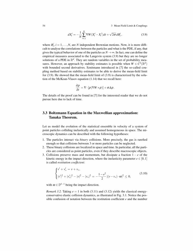
54 3 Mean Field Limit & Couplings
dX it =−
1N
N
∑i6= j
∇W (X it −X j
t )dt +√
2σ dBit , (3.9)
where Bit , i = 1, . . . ,N, are N independent Brownian motions. Now, it is more diffi-
cult to analyse the correlations between the particles and what is the PDE, if any, thatgives the typical behavior of one of the particles as N→∞. In fact, one can define theempirical measures associated to the Langevin system (3.9) but they are no longersolutions of a PDE in Rd . They are random variables in the set of probability mea-sures. However, an approach by stability estimates is possible when W ∈ C2(Rd)with bounded second derivatives. Sznitmann introduced in [7] the so-called cou-pling method based on stability estimates to be able to derive the mean-field limitfor (3.9). He showed that the mean-field limit of (3.9) is characterized by the solu-tion of the McKean-Vlasov equation (1.14) that we recall here:
∂ρ
∂ t= ∇ · [ρ(∇W ∗ρ)]+σ∆ρ.
The details of the proof can be found in [7] for the interested reader that we do notpursue here due to lack of time.
3.3 Boltzmann Equation in the Maxwellian approximation:Tanaka Theorem.
Let us model the evolution of the statistical ensemble in velocity of a system ofpoint particles colliding inelastically and assumed homogeneous in space. The mi-croscopic dynamics can be described with the following hypotheses:
1. The particles interact via binary collisions. More precisely, the gas is rarefiedenough so that collisions between 3 or more particles can be neglected.
2. These binary collisions are localized in space and time. In particular, all the parti-cles are considered as point particles, even if they describe macroscopic objects.
3. Collisions preserve mass and momentum, but dissipate a fraction 1− e of thekinetic energy in the impact direction, where the inelasticity parameter e ∈ [0,1]is called restitution coefficient:
v′ + v′∗ = v + v∗,
|v′|2 + |v′∗|2 − |v|2 − |v∗|2 = −1− e2
2|(v− v∗) ·ω|2 ≤ 0,
(3.10)
with ω ∈ Sd−1 being the impact direction.
Remark 3.2. Taking e = 1 in both (3.11) and (3.12) yields the classical energy-conservative elastic collision dynamics, as illustrated in Fig. 3.1. Notice the pos-sible confusion of notation between the restitution coefficient e and the number
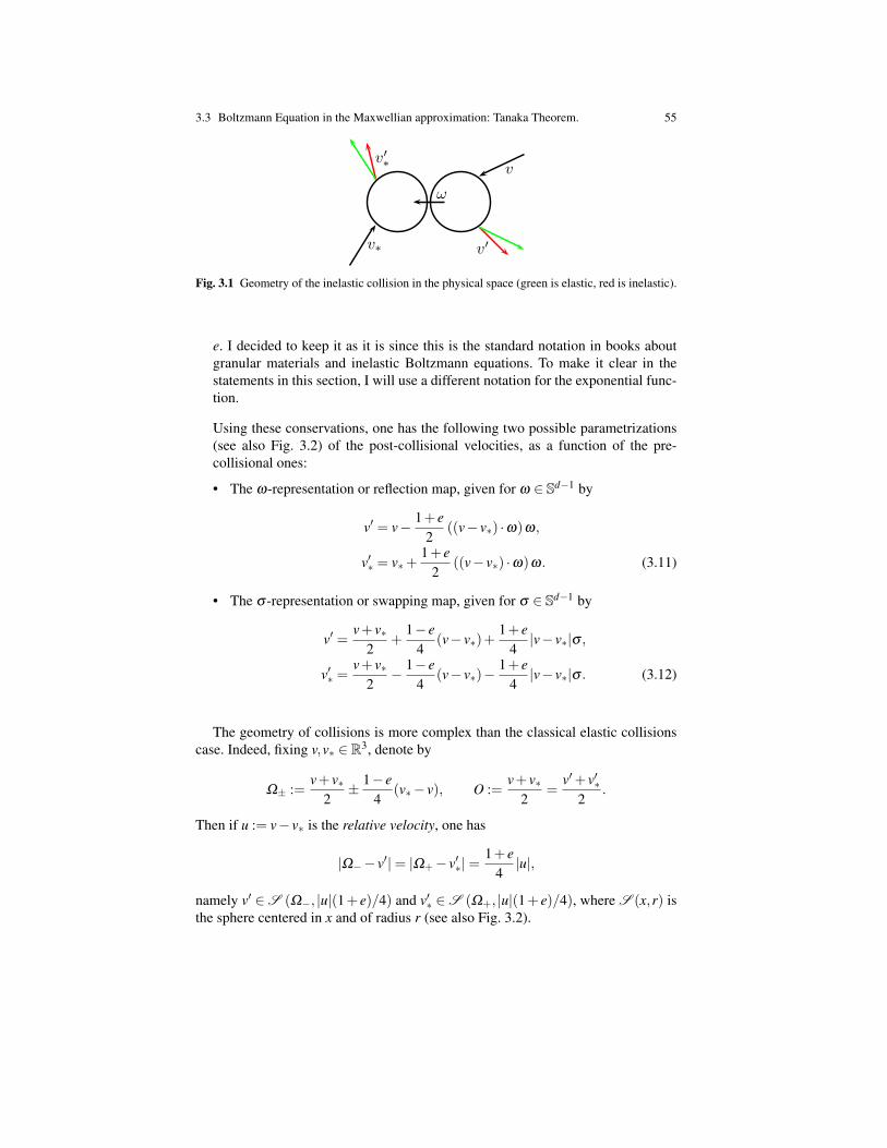
3.3 Boltzmann Equation in the Maxwellian approximation: Tanaka Theorem. 55
ω
v
v∗
v′∗
v′
Fig. 3.1 Geometry of the inelastic collision in the physical space (green is elastic, red is inelastic).
e. I decided to keep it as it is since this is the standard notation in books aboutgranular materials and inelastic Boltzmann equations. To make it clear in thestatements in this section, I will use a different notation for the exponential func-tion.
Using these conservations, one has the following two possible parametrizations(see also Fig. 3.2) of the post-collisional velocities, as a function of the pre-collisional ones:
• The ω-representation or reflection map, given for ω ∈ Sd−1 by
v′ = v− 1+ e2
((v− v∗) ·ω)ω,
v′∗ = v∗+1+ e
2((v− v∗) ·ω)ω. (3.11)
• The σ -representation or swapping map, given for σ ∈ Sd−1 by
v′ =v+ v∗
2+
1− e4
(v− v∗)+1+ e
4|v− v∗|σ ,
v′∗ =v+ v∗
2− 1− e
4(v− v∗)−
1+ e4|v− v∗|σ . (3.12)
The geometry of collisions is more complex than the classical elastic collisionscase. Indeed, fixing v,v∗ ∈ R3, denote by
Ω± :=v+ v∗
2± 1− e
4(v∗− v), O :=
v+ v∗2
=v′+ v′∗
2.
Then if u := v− v∗ is the relative velocity, one has
|Ω−− v′|= |Ω+− v′∗|=1+ e
4|u|,
namely v′ ∈S (Ω−, |u|(1+ e)/4) and v′∗ ∈S (Ω+, |u|(1+ e)/4), where S (x,r) isthe sphere centered in x and of radius r (see also Fig. 3.2).
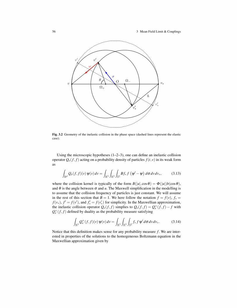
56 3 Mean Field Limit & Couplings
bv b v∗bO
b
Ω+
bΩ−
bv′
b
v′∗
bv′
b v′∗
θσ
h
ω
Fig. 3.2 Geometry of the inelastic collision in the phase space (dashed lines represent the elasticcase).
Using the microscopic hypotheses (1–2–3), one can define an inelastic collisionoperator Qe( f , f ) acting on a probability density of particles f (t,v) in its weak formas ∫
RdQe( f , f )(v)ψ(v)dv =
∫R3
∫R3
∫S2
B f∗ f(ψ′−ψ
)dσ dvdv∗, (3.13)
where the collision kernel is typically of the form B(|u|,cosθ) = Φ(|u|)b(cosθ),and θ is the angle between σ and u. The Maxwell simplification in the modelling isto assume that the collision frequency of particles is just constant. We will assumein the rest of this section that B = 1. We here follow the notation f = f (v), f∗ =f (v∗), f ′ = f (v′), and f ′∗ = f (v′∗) for simplicity. In the Maxwellian approximation,the inelastic collision operator Qe( f , f ) simplies to Qe( f , f ) = Q+
e ( f , f )− f withQ+
e ( f , f ) defined by duality as the probability measure satisfying∫R3
Q+e ( f , f )(v)ψ(v)dv =
∫R3
∫R3
∫S2
f∗ f ψ′ dσ dvdv∗. (3.14)
Notice that this definition makes sense for any probability measure f . We are inter-ested in properties of the solutions to the homogeneous Boltzmann equation in theMaxwellian approximation given by

3.3 Boltzmann Equation in the Maxwellian approximation: Tanaka Theorem. 57
∂ f∂ t
= Qe( f , f ) = Q+e ( f , f )− f . (3.15)
The basic properties of solutions to (3.15) are conservation of mass and mean ve-locity and disipation of the kinetic energy.
In this section, we will analyse the behavior of solutions to (3.15) as curves ofprobability measures in velocity space. Observe though that we will use the notationas if they were densities as it is customary in kinetic equations. We wil not attemptto develop a full well-posedness theory of solutions in these notes but let us focus inunderstanding the main properties of the gain part of the collision operator that onecan use to build the theory of well-posedness and to study the long-time asymptoticproperties of the solutions.
Let us first reinterpret the gain operator: given a probability measure f on R3, thegain operator is the probability measure Q+
e ( f , f ) defined by
(ϕ,Q+e ( f , f )) =
∫R3
∫R3
f (v) f (v∗)(ϕ,Uv,v∗)dvdv∗
where Uv,v∗ is the uniform probability distribution on the sphere S (Ω−, |u|(1+ e)/4).In probabilistic terms, the gain operator is defined as an expectation:
Q+e ( f , f ) = E [UV,V∗ ]
where V and V∗ are independent random variables with law f .
Theorem 3.4 (Contraction of Q+e ( f , f ) in d2). Given f and g in P2(R3) with
equal mean velocity, then
d2(Q+e ( f , f ),Q+
e (g,g))≤√
3+ e2
4d2( f ,g).
Proof. The main steps of the proof can be summarized as follows: Let us take twoindependent pairs of random variables (V,X) and (W,Y ) such that V and W havelaw f and X and Y have law g.
Step 1.- Convexity of d22 in Theorem 2.3 implies
d22(Q
+e ( f , f ),Q+
e (g,g)) = d22(E [UV,W ] ,E [UX ,Y ])≤ E
[d2
2(UV,W ,UX ,Y )]. (3.16)
Here, the independency of the pairs of random variables has been used.Step 2.- The d2
2 distance between the uniform distributions on the sphere withcenter O and radius r, UO,r, and on the sphere with center O′ and radius r′, UO′,r′ ,in R3 is bounded by |O′−O|2 +(r′− r)2.
This is an estimate over the euclidean cost of transporting one sphere onto theother made by explicitly constructing a transport map T , UO′,r′ = T #UO,r. Then,the transport plan ΠT = (1Rd ×T )#UO,r given by∫∫
R3×R3η(v,w)dΠT (v,w) =
∫R3
η(v,T (v))dUO,r(v)
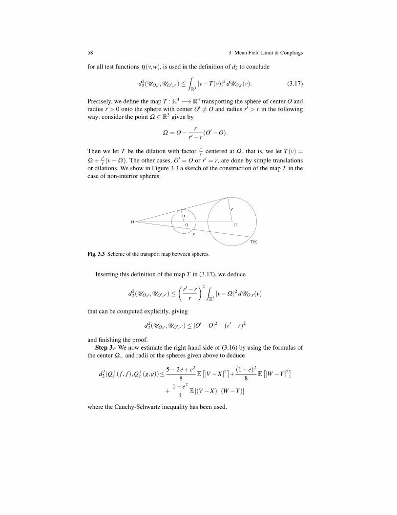
58 3 Mean Field Limit & Couplings
for all test functions η(v,w), is used in the definition of d2 to conclude
d22(UO,r,UO′,r′)≤
∫R3|v−T (v)|2 dUO,r(v). (3.17)
Precisely, we define the map T : R3 −→ R3 transporting the sphere of center O andradius r > 0 onto the sphere with center O′ 6= O and radius r′ > r in the followingway: consider the point Ω ∈ R3 given by
Ω = O− rr′− r
(O′−O).
Then we let T be the dilation with factor r′r centered at Ω , that is, we let T (v) =
Ω + r′r (v−Ω). The other cases, O′ = O or r′ = r, are done by simple translations
or dilations. We show in Figure 3.3 a sketch of the construction of the map T in thecase of non-interior spheres.
O O’
r’
r
Ω
v
T(v)
Fig. 3.3 Scheme of the transport map between spheres.
Inserting this definition of the map T in (3.17), we deduce
d22(UO,r,UO′,r′)≤
(r′− r
r
)2 ∫R3|v−Ω |2 dUO,r(v)
that can be computed explicitly, giving
d22(UO,r,UO′,r′)≤ |O′−O|2 +(r′− r)2
and finishing the proof.Step 3.- We now estimate the right-hand side of (3.16) by using the formulas of
the center Ω− and radii of the spheres given above to deduce
d22(Q
+e ( f , f ),Q+
e (g,g))≤5−2e+ e2
8E[|V −X |2
]+(1+ e)2
8E[|W −Y |2
]+
1− e2
4E [(V −X) · (W −Y )]
where the Cauchy-Schwartz inequality has been used.
3.3 Boltzmann Equation in the Maxwellian approximation: Tanaka Theorem. 59
Step 4.- Finally, we take both pairs (V,X) and (W,Y ) as independent pairs ofvariables with each of them being an optimal couple for the d2( f ,g) to obtain
d22(Q
+e ( f , f ),Q+
e (g,g))≤3+ e2
4d2
2( f ,g)+1− e2
4E [(V −X) · (W −Y )]
=3+ e2
4d2
2( f ,g) ,
due to independency and having equal mean velocity. ut
As a consequence, one can deduce the following property for solutions of theBoltzmann equation in the maxwellian approximation (3.15). We assume here theexistence and uniqueness of solutions to (3.15) as continuous curves in P2(R3)that can be obtained similarly to the previous section based on the estimates on thecontraction of d2 in the previous theorem (this is left as an exercise for e ∈ [0,1)).Since the mean velocity of solutions to (3.15) is conserved, we can assume withoutloss of generality that solutions have zero mean velocity.
Theorem 3.5 (Contraction in d2). If f1 and f2 are two solutions to (3.15) withrespective initial data f 0
1 and f 02 in P2(R3) and zero mean velocity, then
d2( f1(t), f2(t))≤ exp(−αt)d2( f 01 , f 0
2 )
for all t ≥ 0 with α = 1−e2
8 .
Proof. Duhamel’s formula for (3.15) reads as
fi(t) = exp(−t) f 0i +
∫ t
0exp(−(t− s))Q+
e ( fi(s), fi(s))ds, i = 1,2.
As before, the convexity of the squared Wasserstein distance in Theorem 2.3 andthe contraction of the gain operator in Theorem 3.4 imply
d22( f1(t), f2(t))≤ exp(−t)d2
2( f 01 , f 0
2 )
+∫ t
0exp(−(t− s))d2
2(Q+
e ( f1(s), f1(s)),Q+e ( f2(s), f2(s))
)ds
≤ exp(−t)d22( f 0
1 , f 02 )+
3+ e2
4
∫ t
0exp(−(t− s))d2
2( f1(s), f2(s))ds.
Gronwall’s lemma concludes the proof. ut
Notice that Theorem 3.5 does not give a strict contraction for the classical Boltz-mann equation for Maxwell molecules when e = 1. However, one can improve thisresult by studying the cases of equality in the contraction estimate showing that infact one converges in d2 to the Maxwellian equilibria in d2. This together with thenon strict contraction is called the Tanaka theorem for the Boltzmann equation.

Chapter 4An introduction to Gradient Flows
This chapter is devoted to a brief and partly informal introduction to gradient flowsin the space of probability measures. The objective is to illustrate by means of themost basic examples the main ideas of this approach. This is complemented byformal computations for developing some of the intuitions for applications of thistheory in many areas of modelling from biological problems to problems in big dataor social sciences.
4.1 Brenier’s Theorem and Dynamic Interpretation of optimaltransport.
Let us consider u(t,x) a bounded smooth vector field in Rd meaning that u isbounded and globally Lispchitz in x and continuous in t, we can apply the Cauchy-Lispchitz theory to have a well defined flow map associated to u(t,x) satisfying
drds
= u(s,r) in 0≤ s≤ 1,
r(0) = x ∈ Rd .
We denote the flow map by Φt . Reproducing the proof in the first section ofChapter 3, one can show that given ρ0 ∈ P2(Rd), the unique weak solution inC([0,1],P2(Rd)) of the continuity equation
∂sρ +∇ · (ρu) = 0 in (0,1)×Rd (4.1)
is given by ρ(s) = Φs#ρ0 ∈C([0,1],P2(Rd)). Given a pair of a curve of probabilitymeasures and a velocity field (ρ,u) satisfying the continuity equation (4.1) in thedistributional sense, we can define its action as
61

62 4 An introduction to Gradient Flows
A [ρ,u] :=∫ 1
0
∫Rd|u(s,x)|2 dρ(s)(x)ds .
The following remarkable formula is due to Benamou and Brenier giving an alter-native characterization of the d2 distance in terms of the path joining two probabilitymeasures through the continuity equation (4.1) with the minimal kinetic energy.
Theorem 4.1. Given probability measures µ,ν ∈P2(Rd), then
d22(µ,ν) = inf
(ρ,u)
A [ρ,u] : (ρ,u) satisfying (4.1) and ρ0 = µ and ρ1 = ν
holds.
Proof. We give a formal proof since a full proof goes beyond the scope of this in-troductory course. Given an admissible pair (ρ,u) of a curve in C([0,1],P2(Rd))and a smooth velocity field satisfying (4.1), ρ0 = µ , and ρ1 = ν , we discussed abovethat the curve can be expressed in terms of the flow map as ρ(s) = Φs#ρ0. In partic-ular, Φ1 is a transport map from µ to ν . By definition of push-forward and Holder’sinequality we obtain
A [ρ,u] =∫ 1
0
∫Rd|u(s,x)|2 dρ(s)(x)ds =
∫ 1
0
∫Rd|u(s,Φs(x))|2 dρ0(x)ds
=∫ 1
0
∫Rd
∣∣∣∣dΦs(x)ds
∣∣∣∣2 dρ0(x)ds =∫Rd
∫ 1
0
∣∣∣∣dΦs(x)ds
∣∣∣∣2 dsdρ0(x)
≥∫Rd
∣∣∣∣∫ 1
0
dΦs(x)ds
ds∣∣∣∣2 dρ0(x) =
∫Rd|Φ1(x)− x|2 dρ0(x)≥ d2
2(µ,ν) .
Hence, d22(µ,ν) is less or equal than the infimum in the statement.
To show equality, assume that the target measure µ ÎL , then we can use Bre-nier’s Theorem 2.6 to have a well defined transport map leading to the optimalcost for d2
2(µ,ν), i.e., ν = T #µ and the optimal transference plan is of the formΠo = (1Rd ×T )#µ ∈Γ (µ,ν). Then, define Ts(x) = (1− s)x+ sT (x) and choose thevelocity field such that dTs(x)
ds = u(s,Ts(x)). Then, one can easily checked that all theabove inequalities become identities, and thus the infimum is achieved. We leave asan exercise to show that u(s,x) is well defined by proving that Ts(x) in invertible andLispchitz for 0≤ s< 1 using that T = ∇ϕ with ϕ convex. ut
This dynamic interpretation of the transport distance has been crucial both fromthe theoretical and numerical viewpoints. It has led to connections to fluid mechan-ics and to computational transport tools based on optimization methods and numer-ical approximation of PDEs. It is also crucial to interpret the family of general PDE(1.1) as gradient flows as we will see in the last section. It was a key element foran interpretation of the tangent to a curve of probability measures as introduced byOtto in the seminal work [16] and the nowadays known as Otto’s calculus. We donot have time to cover this aspect of the theory.

4.2 McCann’s Displacement Convexity: Internal, Interaction and Confinement Energies. 63
4.2 McCann’s Displacement Convexity: Internal, Interactionand Confinement Energies.
We will start by constructing geodesics between probabilty measures with generaltransport distances dp, 1≤ p< ∞.
Lemma 4.1. [Geodesics] Given probability measures µ,ν ∈Pp(Rd), 1 ≤ p < ∞.Given Π ∈ Γ (µ,ν) an optimal plan for dp(µ,ν), define µt = Tt#Π with the mapTt : Rd×Rd −→ Rd given by Tt(x,y) = (1− t)x+ ty. Then, µt is a constant speeddp geodesic curve joining µ to ν , that is,
dp(µs,µt) = |t− s|dp(µ0,µ1) = |t− s|dp(µ,ν) for all 0≤ s≤ t ≤ 1 .
Proof. Since Π ∈ Γ (µ,ν), it is obvious that µ0 = µ and µ1 = ν . Moreover, takingthe plan Πs,t = (Ts,Tt)#Π ∈ Γ (µs,µt), we get
dpp(µs,µt)≤
∫Rd×Rd
|x− y|p dΠs,t(x,y)
=∫Rd×Rd
|Ts(x)−Tt(y)|p dΠ(x,y) = |t− s|pdpp(µ,ν).
If we use this estimate now on the intervals [0,s], [s, t] and [t,1], we get
dp(µ,µs)+dp(µs,µt)+dp(µt ,ν)≤ (s+ t− s+1− t)dp(µ,ν) = dp(µ,ν) .
Notice that the reverse inequality is always true due to the triangular inequality sincedp is a metric, then all the inequalities in between must be equalities, and thus theclaim of the Lemma is true. ut
Notice that any optimal coupling for dp(µ,ν) generates a constant speed geodesicjoining the measures. In case the optimal transference plan is given by an opti-mal map as in Brenier’s Theorem 2.6, i.e., the optimal transference plan is of theform Πo = (1Rd ×T )#µ ∈ Γ (µ,ν), then the geodesic is given by µt = Tt#µ withTt(x) = (1− t)x+ tT (x) and ν = T #µ . In other words, the geodesic is obtained bypushing-forward the density through the linear interpolant of the identity map andthe optimal transport map T between the measures µ and ν . Remember we alreadydiscussed an application of these interpolants between measures in “image process-ing” in Figure 2.2.
We have already seen that convexity properties of functionals are very importantto understand the dynamics of PDEs of the form (1.1) in various particular cases.Based on the geodesics in transport distances, we can now introduce a notion ofconvexity that plays an important role in the understanding of gradient flows inprobability measures as we will see in the next section.
Definition 4.1 (Displacement Convexity). We say that a functional F : P2(Rd)−→R∪ +∞ is d2-convex or displacement convex, if the one dimensional function

64 4 An introduction to Gradient Flows
F [µt ] is convex in t ∈ [0,1] for all d2 geodesics µt joining any two measuresµ,ν ∈P2(Rd), that is,
F [µt ]≤ (1− t)F [µ0]+ tF [µ1]
for all d2 geodesics µt .
Assume that U : [0,∞) → R is a C([0,∞),R) ∩C2((0,∞),R) function withU(0) = 0, V : Rd → R is a bounded below confinement potential and W : Rd → Ris a bounded below interaction potential as defined in Chapter 1. Associated to thePDE (1.1), we define the following functionals: internal, confinement, and interac-tion energy U ,V ,W : P2(Rd)−→ R∪+∞, as
U (ρ) =∫Rd
U(ρ)dx , (4.2)
if µ ÎL with density ρ and U =+∞ otherwise,
V [µ] =∫Rd
V (x)dµ(x) , (4.3)
andW [ρ] =
12
∫Rd×Rd
W (x− y)dµ(x)dµ(y). (4.4)
Lemma 4.2 (Convexity of confinement and interaction energies). If V : Rd → Ris convex then the confinement energy V is d2-convex. If W : Rd→R is convex thenthe confinement energy W is d2-convex. Morever, if V is strictly convex then V isstrictly d2-convex., and if W is strictly convex then W is strictly d2-convex unlessthe geodesic joining the measures is a translation of a given measure.
Proof. Given probability measures µ,ν ∈P2(Rd), any d2-geodesic joining them isof the form µt =Tt#Π with Π ∈Γ (µ,ν) an optimal plan for d2(µ,ν). We can nowcompute the values of the confinement and interaction energies on the geodesic toget
V [µt ] =∫Rd
V (x)dµt(x) =∫Rd×Rd
V ((1− t)x+ ty)dΠ(x,y)
and
W [µt ] =12
∫Rd×Rd
W (x− y)dµt(x)dµt(y)
=12
∫Rd×Rd
∫Rd×Rd
W ((1− t)(x− y)+ t(z−w))dΠ(x,z)dΠ(y,w) .
Using the convexity of V and W in the integrands above implies immediately thefirst statements of the lemma. The strictly convex claims are an exercise. ut
We now focus on the internal energy. Since the internal energy is infinite unlessthe measure is absolutely continuous with respect to the Lebesgue measure, we

4.2 McCann’s Displacement Convexity: Internal, Interaction and Confinement Energies. 65
can reduce to the case of a geodesic joining two absolutely continuous measuresµ,ν ∈P2(Rd) with respect to Lebesgue, otherwise there is nothing to prove. In thiscase, we can use Brenier’s Theorem 2.6 to write ν =∇ϕ#µ with ϕ a convex functionand the geodesic as µt = Tt#µ with Tt(x) = (1− t)x+ t∇ϕ(x). Let us denote byρt(x) the density of the measure µt with respect to Lebesgue. If the convex functionϕ were C2 and the map ∇ϕ a diffeomorphism, we could use change of variables towrite the internal energy as
U [µt ] =∫Rd
U(ρt(x))dx =∫
ρt>0
U(ρt(x))ρt(x)
ρt(x)dx
=∫
ρ0>0
U((ρt Tt)(x))(ρt Tt)(x)
ρ0(x)dx =∫
ρ0>0U(
ρ0(x)det∇Tt(x)
)det∇Tt(x)dx
=∫Rd
U(
ρ0(x)det((1− t)Id + tD2ϕ(x))
)det((1− t)Id + tD2
ϕ(x))dx .
In these identities, we formally used the change of variables formula in the push-forward as Exercise 5 in Problem Sheet 1. Now, convex analysis again comes tohelp us. Since ϕ is a convex function, it is differentiable almost everywhere and ithas distributional second derivatives in the Aleksandrov sense with a hessian matrixD2ϕ that is a symmetric and nonnegative measure. Moreover, the previous change ofvariables formula makes sense, we refer to [21, Chapter 4] for further details. Usingthe notation D(x, t) = det((1− t)Id + tD2ϕ(x))1/d , we have finally shown that
U [µt ] =∫Rd
U(
ρ0(x)D(x, t)d
)D(x, t)d dx.
We leave as an exercise to show the following lemma.
Lemma 4.3. Let Λ be a nonnegative symmetric matrix and v(t) = det((1− t)Id +tΛ)1/d . Then v is concave on t ∈ [0,1] and strictly concave unless Λ = λ Id .
Applying this to D(x, t), we deduce that D(x, t) is concave in t for all x ∈ Rd .Moreover, defining G(x,s) = sdU(ρ0(x)s−d) for s > 0, we can write the internalenergy of the geodesic as
U [µt ] =∫Rd
G(x,D(x, t))dx.
Assume that the function g(s) = sdU(s−d), s> 0, is convex and nonincreasing, thenit is left as an exercise to show that the map t −→ G(x,D(x, t)) is a convex functionin t for all x ∈ Rd , and thus the internal energy of the geodesic is convex in t. Wehave shown the so-called McCann’s condition for displacement convexity of theinternal energy.
Theorem 4.2. [McCann’s condition] Assume U : [0,∞) → R is a C([0,∞),R) ∩C2((0,∞),R) function with U(0) = 0 such that sdU(s−d), s> 0, is convex and non-increasing, then the internal energy U is d2-convex.

66 4 An introduction to Gradient Flows
Particular important choices of internal energies satisfying the McCann’s con-dition are the Boltzmann entropy with U(s) = s log(s) and the power-law caseU(s) = sm for all m≥ 1− 1
d , m 6= 1. We leave as an exercise to check that U satisfiesthe McCann’s condition if and only if P(s) ≥ 0 and (1− 1
d )P(s) ≤ sP′(s) for alls> 0 with P defined from U by sU ′′(s) = P′(s) and P(0) = 0.
We will now learn how to obtain these conditions from the dynamic interpretationseen in the previous section in a formal way by computing optimality conditions.Given µ,ν ∈P2(Rd), we first obtain the optimality condition for the geodesic equa-tions in the fluid dynamical formulation of the d2 distance by the Benamou-Brenierformula in Theorem 4.1. We insert the continuity equation
∂sρ +∇ · (ρu) = 0 in (0,1)×Rd (4.5)
inside the minimization problem as a Lagrange multiplier in its weak form using atest function ψ ∈C∞
o ([0,1]×Rd). As a result, we get the unconstrained minimizationproblem
12
d22(µ,ν) = inf
(ρ,u)sup
ψ
∫ 1
0
∫Rd
12|us(x)|2ρs(x) dxds
−∫ 1
0
∫Rd
[ρs(x)∂sψ(s,x)+ρs(x)(us(x) ·∇ψ(s,x))] dxds
+∫Rd
ψ(1,x)dρ1(x)−∫Rd
ψ(0,x)dρ0(x).
The factor 1/2 is for convenience for the computations below. Applying a formalminimax principle, swapping infimum and supremum, and thus taking first an infi-mum with respect to u we obtain the optimality condition u=∇ψ, and the followingformal characterization of the distance
12
d22(µ,ν) = sup
ψ
infρ
− 1
2
∫ 1
0
∫Rd|∇ψ|2ρ dxds−
∫ 1
0
∫Rd
ρ∂sψ dxds
+∫Rd
ψ(1,x)dρ1(x)−∫Rd
ψ(0,x)dρ0(x),
which provides the further optimality condition
∂sψ +12|∇ψ|2 = 0. (4.6)
We thus end up with a coupled system of differential equations in (0,1)×Rd asoptimality conditions for the geodesic curves in the dynamic formulation
∂sρ +∇ · (ρ∇ψ) = 0,
∂sψ +12|∇ψ|2 = 0,
(4.7)

4.2 McCann’s Displacement Convexity: Internal, Interaction and Confinement Energies. 67
together with the boundary conditions ρ0 = µ and ρ1 = ν . Let us now use the for-mal equations (4.7) for the geodesics associated to the distance d2 to compute theconditions under which the internal energy functional is displacement convex. As-suming (ρs,ψs) is a smooth solution of (4.7), which decays sufficiently at infinity,we proceed by integration by parts to obtain the following formulas:
dds
U [ρ] =−∫Rd
P(ρ)∆ψ dx,
with P defined by P′(r) = rU ′′(r) and P(0) = 0. Furthermore, one can further com-pute to obtain
d2
ds2 U [ρ] =∫Rd(P′(ρ)ρ−P(ρ))(∆ψ)2 dx
+∫Rd
P(ρ)(−∇ψ ·∇∆ψ +12
∆ |∇ψ|2) dx.
The Bochner formula implies that
−∇ψ ·∇∆ψ +12
∆ |∇ψ|2 = |D2ψ|2 = trace
[(D2
ψ)2]≥ 1
d(∆ψ)2 =
1d
[trace(D2
ψ)]2,
the last inequality using the fact that D2ψ is a symmetric matrix. Assuming thatP(ρ)≥ 0, we can estimate it as
d2
ds2 U [ρ]≥∫Rd(P′(ρ)ρ− (1−1/d)P(ρ))(∆ψ)2 dx.
Therefore, under the displacement McCann’s condition, P(s)≥ 0 and (1− 1d )P(s)≤
sP′(s) for all s > 0 with P defined from U by sU ′′(s) = P′(s) and P(0) = 0, thefunctional U is convex along the geodesics of the distance d2 based on these formalcomputations. This is a very useful procedure to guess the convexity properties offunctionals. Let us do a similar computation for the confinement energy V . Theformulas of the first and second derivatives along geodesics satisfying (4.7) are
dds
V [ρ] =∫Rd
ρ∇V ·∇ψ dx,
andd2
ds2 V [ρ] =∫Rd
ρ (D2V ∇ψ) ·∇ψ dx .
Again, we observe that if V is convex, D2V ≥ 0 and we have displacement convexityof V . Moreover, this computation shows that if V is 2-uniform convex, i.e., D2V ≥λ Id for λ > 0, then
68 4 An introduction to Gradient Flows
d2
ds2 V [ρ]≥ λ
∫Rd
ρ |∇ψ|2 dx = λd22(µ,ν) .
This leads to a definition of 2-uniform displacement convexity for functionals inprobability measures. We leave as exercise to use the same procedure for analysingthe convexity of the interaction energies W .
In fact, this approach can be generalized to find formal optimality conditionsfor many different variants of transport distances defined by the dynamical formu-lation introduced in Theorem 4.1. Examples of these variants are nonlinear con-tinuity equations with different mobility functions, nonlocal mobilities, fractionaldiffusions, the Landau equation in plasma physics, the relativistic heat equation andmany other partial differential equations can be connected in this way to variants ofthese transport distances.
4.3 Gradient Flows: the differential viewpoint.
Before attempting to construct an abstract argument in a context fraught with perilsof nonsmoothness, infinite dimensions, and degenerate convexity, it is instructive torecall basic ideas about gradient flows. The setting will be so simple that not onlyare the results well-known, they could all be deduced by a good sophomore calculusstudent. Fix E ∈C2(Rd) and consider solutions of the ordinary differential equation
dxt
dt=−∇E(xt) (4.8)
corresponding to steepest descent or gradient flow on the energy (entropy) landscapedetermined by E. Solutions satisfy
ddt
E(xt) =−|∇E(xt)|2 , (4.9)
and thus the energy decays along the curves xt solutions to (4.8). Moreover, theenergy E is a strict Liapunov functional in the sense that d
dt E(xt) = 0 if and only ifxt is a critical point of E.
Lemma 4.4 (Bounding contraction / expansion rates). Fix λ ∈ R. If E ∈C2(Rd)satisfies D2E(x)≥ λ Id throughout Rd , and the curves xt and t ∈ [0,∞)−→ yt ∈ Rd
both solve the differential equation (4.8), then |xt − yt | ≤ e−λ t |x0− y0|.Proof. Set f (t) = |xt − yt |2/2. Then
f ′(t) =−< xt − yt ,∇E(xt)−∇E(yt)>
=−< xt − yt ,∫ 1
0D2E[(1− s)xt + syt ] (yt − xt)ds>≤−2λ f (t)
∫ 1
0ds.
Gronwall’s inequality (integration) implies the desired result: f (t)≤ e−2λ t f (0). ut

4.3 Gradient Flows: the differential viewpoint. 69
Corollary 4.1 (Contraction in a convex valley). Taking λ = 0 in the precedingproposition implies |xt − yt | is monotone nonincreasing as a function of t ∈ [0,∞).
Proof. Obviously |xt−yt | ≤ |x0−y0|. Since the equation is autonomous, time trans-lation invariance implies |xT+t − yT+t | ≤ |xT − yT | for all t,T ≥ 0. ut
If λ > 0, more can be achieved. The convexity of E is said to be 2-uniform,and we have shown that the solution map x0 ∈ Rd −→ Xt(x0) = xt of the initialvalue problem (4.8) defines a uniform contraction on Rd for each t > 0. The C2
smoothness of E ensures that the solution map is well-defined locally in space andtime; the map is globally defined for all future times since xt is constrained to liein the level set x | E(x) ≤ E(x0), whose compactness follows from the coerciv-ity of E(x) ≥ E(x0)+ < ∇E(x0),x− x0 > +λ |x− x0|2/2. Since Rd is complete,the contraction mapping principle dictates that this map has a unique fixed pointXt(x∞) = x∞ ∈ Rd , and each solution curve xt = Xt(x0) must converge to x∞ inthe long time limit t → ∞. The quantity estimated is the decay rate of the slope|∇E(xt)| → 0, that we can call the information.
Lemma 4.5 (Entropy production and information decay rate). Let E ∈C2(Rd)satisfy D2E(x) ≥ λ Id > 0 throughout Rd . Then any solution t ∈ [0,∞) −→ xt ∈ Rd
of (4.8) satisfies |∇E(xt)| ≤ e−λ t |∇E(x0)|.
Proof. Let f (t) := |∇E(xt)|2/2. Then
f ′(t) =< ∇E(xt),D2E(xt) xt >=−< ∇E(xt),D2E(xt)∇E(xt)>≤−2λ f (t),
and Gronwall’s inequality proves the desired estimate: f (t)≤ e−2λ t f (0). ut
While the conclusions of these two lemmas are not immediately comparable,the following consequence (4.10) of 2-uniform convexity relates them. It showsthat information dominates the altitude or relative entropy E(x)−E(x∞), which inturn dominates horizontal distance squared. Thus in its limited range of validity —λ > 0 and yt := x∞ — and apart from constants, Proposition 4.5 trumps Proposi-tion 4.4. On the other hand, (4.11) also shows that if information remains bounded,then convergence in the weakest sense, namely of distance (unsquared), also impliesconvergence in the stronger sense of relative entropy.
Lemma 4.6 (Manifestations of 2-uniform convexity). Let 0 ≤ f ∈ C2(R) satisfyf (0) = 0 and f ′′(s)> λ > 0 for all s ∈ R. Then λ s2 ≤ 2 f (s)≤ λ−1| f ′(s)|2 and
f (s)≤ s f ′(s)−λ s2/2.
Proof. Let g(s) := f (s)−λ s2/2. Taking two derivatives shows g(s) is convex, soits critical point at the origin must be a minimum: g(s)≥ g(0) = 0. This proves thefirst inequality.
Since f (s)≥ 0 is strictly convex, its minimum f (0) = 0 is its only critical point.Defining h(s) := | f ′(s)|2/2−λ f (s), we see h′(s)= f ′(s)( f ′′(s)−λ ) can vanish onlywhere f ′(s) does — namely, at zero. Since h′′(0) = f ′′(0)( f ′′(0)−λ )+0 f ′′′(0) >
70 4 An introduction to Gradient Flows
0, the unique critical point of h(s) is a strict local minimum; it must be a globalminimum since the absence of other critical points ensures that monotonicity of h(s)changes only at zero. Thus h(s)≥ h(0) = 0, which establishes the second inequality.
Finally, let e(s) = s f ′(s)− λ s2/2− f (s). Then e′(s) = s( f ′′(s)− λ ) vanishesonly when s = 0. A second derivative e′′(0) = f ′′(0)− λ > 0 shows this uniquecritical point of e(s) to be a strict local minimum, hence a global minimum as above:e(s)≥ e(0) = 0 to complete the proof of the lemma. ut
Corollary 4.2 (Cartoon Log Sobolev, Talagrand, and HWI inequalities). Sup-pose E(x∞)≤ E(x) ∈C2(Rd) and D2E(x)≥ λ Id > 0 for all x ∈ Rd . Then
λ
2|x− x∞|2 ≤ E(x)−E(x∞) ≤
12λ|∇E(x)|2 (4.10)
and E(x)−E(x∞) ≤ |x− x∞||∇E(x)|−λ |x− x∞|2/2. (4.11)
As a consequence, any solution t ∈ [0,∞) −→ xt ∈ Rd of (4.8) satisfies E(xt)−E(x∞)≤ e−2λ t(E(x0)−E(x∞)).
Proof. The conclusions of the lemma continue to hold under the relaxed hypothesisf (s) ≥ λ , as is easily seen by replacing λ with λ − 1/n and taking a limit n→ ∞.Given x ∈Rd , the function f (s) := E(x∞ + s x−x∞
|x−x∞| )−E(x∞) satisfies the hypothesisf ′′(s) ≥ λ . Setting s = |x− x∞| in the conclusion of the lemma, Cauchy-Schwarzyields the desired inequalities (4.10–4.11). Notice that (4.10) together with (4.9)and Gronwall’s lemma leads to the exponential decay of the relative energy. ut
These intuitions can be applied to particular cases of the general PDE equation(1.1). In particular, let us consider the case of the linear Fokker-Planck equation(1.12) with W = 0, P(ρ) = σρ and V such that D2V (x)≥ λ Id with λ > 0, that is,
∂ρ
∂ t= ∇ · (ρ∇V )+σ∆ρ, (4.12)
We already proved in Section 1.2 that
d2(ρ1(t),ρ2(t))≤ e−λ td2(ρ1(0),ρ2(0))
for any two solutions of (4.12) based on the definition of d2 in terms of randomvariables. However, the deeper reason is that this equation has a “gradient flow”structure in the following sense. Defining the total free energy of the system as
F [ρ] = σ
∫Rd
ρ logρ dx+∫Rd
V (x)ρ dx , (4.13)
we can compute formal variations of the functional around a density ρ ∈ L1+(Rd) by
taking perturbations in the set
S := v ∈ L1(Rd)with zero mean such that ρ + ε v≥ 0 for ε > 0 small enough .

4.3 Gradient Flows: the differential viewpoint. 71
By doing so and assuming the necessary conditions to apply the dominated conver-gence theorem, we obtain
limε→0
F [ρ + ε v]−F [ρ]
ε=∫Rd
δF
δρ(ρ)v dx
with δFδρ
(ρ) := σ log(ρ)+V . Therefore, the linear Fokker-Planck equation can bewritten as
∂sρ +∇ · (ρu) = 0 in (0,∞)×Rd
u =−∇δF
δρ
, (4.14)
where we eliminated the dependence of the variation of F in ρ to ease the notation,we will do so in the sequel when there is no confusion. The free energy (4.13) is aLiapunov functional for (4.12) since
ddt
F [ρ] =−I[ρ] :=−∫Rd
∣∣∣∣∇δF
δρ
∣∣∣∣2 ρ(x)dx , (4.15)
at least by formal integration by parts. Notice that this identity resembles the decayof the energy E in the finite dimensional case, and thus the right hand side shouldbe dissipated by the squared norm of the gradient of the energy if this were a realgradient flow. Here, we observe the connection to the dynamical interpretation of thesquared Wassertein distance d2 in Theorem 4.1. The right hand side is the opossiteof the kinetic energy associated to the vector field −∇
δFδρ
. As mentioned in theprevious section, this is the starting point for a much deeper connection formallyintroduced by Otto in [16]. The resemblance of the linear Fokker-Planck equation(4.12) to the case of 2-uniform gradient flows in finite dimensions goes further. Aswe showed in Section 1.2, the function
ρ∞(x) =1Z
e−V (x)/σ with Z =∫Rd
e−V (x)/σ dx,
is a steady state of (4.12). Notice that δFδρ
(ρ∞) = σ log(ρ∞)+V is constant. There-fore, we can define the relative free energy as F (ρ|ρ∞) = F [ρ]−F [ρ∞] that sat-isfies
F [ρ|ρ∞] = σ
∫Rd
η logη ρ∞ dx ,
with η = ρ/ρ∞. A simple application of Jensen’s inequality with respect to theGaussian measure ρ∞ using that x logx is convex gives
F [ρ]−F [ρ∞]≥ σ
(∫Rd
η ρ∞ dx)
log(∫
Rdη ρ∞ dx
)= 0
and the equality holds if and only if η = 1. Therefore, the Gaussian ρ∞ is the globalminimum of the functional F [ρ]. Moreover, due to the results of the previous sec-

72 4 An introduction to Gradient Flows
tion, the free energy functional F [ρ] is 2-uniform d2 displacement convex sinceit is the sum of a displacement convex functional with a 2-uniform displacementfunctional. So, we are in the best of the worlds, a uniforly convex functional with aglobal minimum but in the displacement sense in the Wasserstein metric space.
A very detailed theory for gradient flows for 2-uniform displacement convexfunctionals has been developed [3, 22, 2]. The theory of 2-uniform d2 gradient flowsapplies and it leads to the following conclusions for the linear Fokker-Planck equa-tion. One can show the following functional inequalities known as the Log-Sobolev,the Talagrand, and the HWI inequalities:
F [ρ|ρ∞]≤1
2λI[ρ] , (4.16)
d2(ρ,ρ∞)≤√
2λ
F [ρ|ρ∞] , (4.17)
and
F [ρ|ρ∞]≤ d2(ρ,ρ∞)√
I[ρ]− λ
2d2
2(ρ,ρ∞). (4.18)
The name of HWI for (4.18) comes from the H-theorem of the Boltzmann entropy,W for Wasserstein distance, and I for the Fisher information functional I[ρ] ascoined by C. Villani. All of them are manifestations of the uniform convexity inthis infinite dimensional setting and they correspond to the results in Corollary 4.2in disguise. These inequalities imply directly a convergence rate towards the steadystate ρ∞ in relative entropy and d2 sense. Just make use of (4.16) in (4.15) to deducethat
ddt
F [ρ|ρ∞] =−I[ρ]≤−2λF [ρ|ρ∞]
giving by Gronwall’s Lemma the exponential decay F [ρ|ρ∞] ≤ e−2λ tF [ρ0|ρ∞],and then Talagrand’s inequality (4.17) to deduce the exponential decay of d2(ρ,ρ∞).However, the 2-uniform displacement convexity of F [ρ] implies a further conse-quence, the uniform contraction in d2 for solutions of (4.12) as proven in Section1.2. This is a general property for this type of gradient flows [3, 22]. Finally, noticethat the general family of PDEs (1.1) introduced in the first chapter of this coursecan be written formally in the form of a gradient flow as in (4.14) with the free en-ergy given by F [ρ] = U [ρ]+V [ρ]+W [ρ] for a suitable function U related to toP, we leave this as an exercise.
4.4 Gradient Flows: the metric viewpoint
Let us come back to the case of gradient flows in Rd . Given E ∈C2(Rd), we considerthe gradient flow dxt
dt =−∇E(xt) for which solutions satisfy (4.9)

4.4 Gradient Flows: the metric viewpoint 73
ddt
E(xt) =−|∇E(xt)|2 .
The previous formula encodes important ingredients for gradient flows. We observethe enery decays the fastest at each point xt of the trajectory, since the energy decaysthe fastest in the direction −∇E(xt) at xt . To even being able to write this we needthe notion of gradient of a function. The theory of gradient flows can be generalizedto Hilbert spaces [5]. However, when we want to generalize this theory to the case ofmetric spaces we do not have this notion of gradient defined properly. Even more ourvelocity fields might not be even C1 as we saw in the case of the Barenblatt solutionto the porous medium equation in Chapter 1. Therefore, a different generalizationof gradient flows is needed. A classical way to construct solutions to the gradientflow (4.8) is by discretizing in time via the implicit Euler scheme: given a time step∆ t and an approximation to the solution at time tk = k∆ t, we find the approximationat time tk+1 by solving
xk+1 = xk−∆ t∇E(xk+1) .
It is easy to see that this identitiy is nothing else than the critical point condition forthe following functional
Ek(x) =1
2∆ t|x− xk|2 +E(x) ,
that is, xk+1 is a critical point of the function Ek. Therefore, a natural way to con-struct xk+1 is by looking for a global minimizer of the energy Ek. Assume now thatE is a convex function in Rd , then the critical point is equivalent to
xk+1 = arg minx∈Rd
1
2∆ t|x− xk|2 +E(x)
since Ek is uniformly convex for all ∆ t > 0 and all k. The previous variational char-acterization of the implicit Euler scheme for gradient flows of convex functionsis useful in two ways: the smoothness of E is only needed to characterize criticalpoints and it encodes again the steepest descent primary property of gradient flows.As mentioned before, the smoothness assumption E in C1 is very strong, so let ustake a function E : Rd −→ R∪ ∞ such that is convex and lower semicontinu-ous. Associated to a convex function, we can define its subdifferential as the set ofdirections determining all supporting hyperplanes, that is
∂E(x) :=
y ∈ Rd : E(z)≥ E(x)+< y,z− x> for all z ∈ Rd.
Recall that absolutely continuous functions on an interval are a.e. differentiable withrespect to Lebesgue. Now we have the ingredients to generalize the notion of gradi-ent flow solution.
Definition 4.2. An absolutely continuous curve x : [0,∞) −→ R is a gradient flowsolution with initial data x(0) for the convex and lower semicontinuous energy func-tional E : Rd −→ R∪∞ if
74 4 An introduction to Gradient Flows
−dxdt∈ ∂E(x(t)) for a.e. t > 0 .
It is not difficult to generalize the variational characterization of the implicit Eulerscheme to this setting. This is left as an exercise, that is,
−xk+1− xk
∆ t∈ ∂E(xk+1)
if and only if
xk+1 = arg minx∈Rd
1
2∆ t|x− xk|2 +E(x)
.
This formulation can be easily generalized to Hilbert spaces and it is easy to showthat the variational scheme above is well defined, i.e., it has a minimum for all kand ∆ t. The dificulty lies in showing the convergence as ∆ t → 0 to a solution inthe sense of Definition 4.2. We refer to [5, 2] for more details. Let us do a classicalexample in Hilbert spaces, take H = L2(Rd) and define the energy functional
E [u] :=
12
∫Rd|∇u|2 dx if u ∈ H1(Rd)
+∞ otherwise. (4.19)
It is convex in the classical sense and lower semicontinuous by standard resultsof weak convergence. We claim that ∂E (x) 6= /0 if and only if ∆u ∈ L2(Rd), andin that case ∂E (x) = −∆u. Assume p ∈ ∂E (x), that is, p ∈ L2(Rd) such thatE (v) ≥ E (u)+ < p,v− u >2 with an obvious notation for the L2-scalar product.Take v = u+ εw with w ∈ H1(Rd), then this inequality leads to
12
∫Rd|∇u+ ε∇w|2 dx− 1
2
∫Rd|∇u|2 dx≥ ε
∫Rd
p(x)w(x)dx .
Rearranging the terms and taking ε → 0, we get∫Rd
∇u ·∇wdx≥∫Rd
p(x)w(x)dx ,
for all w ∈ H1(Rd). Taking −w in the previous inequality, we conclude that∫Rd
∇u ·∇wdx =∫Rd
p(x)w(x)dx ,
for all w ∈H1(Rd), and thus by definition ∆u ∈ L2(Rd) and−∆u = p. We leave theconverse argument as exercise. Therefore, we can properly say that the heat equa-tion is the gradient flow of the Dirichlet energy (4.19) with respect to the L2 scalarproduct. One can actually show that the heat equation is the limit of the implicit Eu-ler scheme defining a piecewise continuous interpolants in time for the L2-functionsconstructively obtained by the interative variational scheme

4.4 Gradient Flows: the metric viewpoint 75
uk+1 = arg minx∈L2(Rd)
1
2∆ t‖u−uk‖2
L2(Rd)+E (x)
,
and showing their convergence to the heat equation as ∆ t → 0. This approach wasintroduced by Jordan, Kiderlehrer and Otto [15] to derive the linear Fokker-Planckequation (4.12) as the steepest descent of the free energy (4.13) in the Wassersteind2 sense. More precisely, they showed that by defining a sequence of measures iter-atively by
ρk+1 = arg minρ∈P2(Rd)
1
2∆ td2
2(ρ,ρk)+F [ρ]
for any fixed ∆ t > 0 and any k ∈ N starting with a given measure ρ0 ∈P2(Rd),then a suitable interpolant in time of these measures leads to a curve of measuresρ∆ t converging to the unique solution of (4.12) with initial data ρ0 ∈P2(Rd) as∆ t → 0. We do not have time to cover this proof in this course, but let us at leastshow that the variational scheme is well defined in a simpler setting. Let us considerΩ a bounded smooth domain of Rd , and let us take as energy functional just theBoltzmann entropy functional, that is,
E [ρ] =∫
Ω
ρ logρ dx .
The formal d2-gradient flow of E is the heat equation in Ω with Neumann boundaryconditions. Let us finally show that the variational scheme
ρk+1 = arg minρ∈P2(Ω)
1
2∆ td2
2(ρ,ρk)+E [ρ]
= arg min
ρ∈P2(Ω)
1
2∆ td2
2(ρ,ρk)+∫
Ω
ρ logρ dx
is well defined for any fixed ∆ t > 0 starting from ρ0 ∈P(Ω).
Lemma 4.7. Given ∆ t > 0, for any k ∈ N the functional
Ek[ρ] :=1
2∆ td2
2(ρ,ρk)+E [ρ]
has a minimum in P(Ω) for a given ρk ∈P(Ω).
Proof. Taking a suitably normalized Gaussian as ρ and since x logx≥−1, it is clearthat the functional Ek has a finite infimum in P(Ω). Take a minimizing sequenceρn ∈P(Ω) that is
12∆ t
d22(ρn,ρk)+E [ρn]→ I := inf
ρ∈P2(Ω)
1
2∆ td2
2(ρ,ρk)+E [ρ]
.
Using again x logx≥−1 and that Ω is bounded, we deduce that the sequence

76 4 An introduction to Gradient Flows∫Ω
ρn log+ ρn dx≤C
for n ∈ N, where log+(x) = max(0, log(x)). Given M ∈ N, denote by ρn ∧M :=min(ρn,M). The sequence of cut-off functions ρn∧M is bounded in L∞(Ω), thus byBanach-Alaoglu theorem, it is weakly-* compact in L∞(Ω) for each given M ∈ N.By a standard diagonal argument, we can extract a subsequence, denoted with thesame index to simplify the notation, such that ρn∧M ρM weakly-∗ in L∞(Ω) forall M ∈ N. Define ρ = supM ρM . Notice that ρn ∧M ≤ ρn ∧ (M + 1), and thereforetheir weak-∗ limits are also ordered, so ρM is an increasing sequence in M a.e.x ∈ Rd . By monotone convergence theorem, we deduce that∫
Ω
ρM dx→∫
Ω
ρ dx≤ ∞ .
Furthermore, since ρn ∧M ρM weakly-∗ in L∞(Ω), we have the convergencetesting against L1(Ω) functions, in particular against the constant 1 so∫
Ω
ρn∧M dx→∫
Ω
ρM dx ,
as n→ ∞, and since ρn ∈P2(Ω), then ρM is bounded in L1(Ω), and in particularρ ∈ L1(Ω) and
‖ρM− ρ‖L1(Ω)→ 0
as M→ ∞. Furthermore, we can estimate
‖ρn−ρn∧M‖L1(Ω) =∫
Ω
(ρn−ρn∧M)dx =∫
ρn≥M(ρn−M)dx≤
∫ρn≥M
ρn dx
≤ 1log(M)
∫ρn≥M
ρn log(ρn)dx≤ Clog(M)
,
for M≥ 2, and thus the right hand side goes to 0 as M→∞. Our claim is that ρn ρ
weakly in L1(Ω). Take a test function ϕ ∈ L∞(Ω), then we can estimate∣∣∣∣∫Ω
ρnϕ dx−∫
Ω
ρϕ dx∣∣∣∣≤‖ϕ‖L∞(Ω)‖ρn−ρn∧M‖L1(Ω)+‖ϕ‖L∞(Ω)‖ρM− ρ‖L1(Ω)
+
∣∣∣∣∫Ω
ρMϕ dx−∫
Ω
ρn∧Mϕ dx∣∣∣∣ .
We take the limit as M→∞ and n→∞ in that order on the right hand side since thefirst two terms can be made small by taking M large uniformly in n, and the last onecan be made small by taking n large enough afterwards. Therefore, ρn ρ weaklyin L1(Ω) as claimed. Let us also show that ρ ∈P(Ω). Take the set Nε := x ∈Ω :dist(x,∂Ω)≤ ε. It is obvious that |Nε | ≤Cε and

4.4 Gradient Flows: the metric viewpoint 77∫Nε
ρn dx≤∫
Nε∩ρn≤Rρn dx+
∫Nε∩ρn≥R
ρn dx
≤CRε +1
log(R)
∫Nε∩ρn≥R
ρn log(ρn)dx≤CRε +C
log(R)
for all R> 0, taking R = ε| log(ε)| leads to∫Ω\Nε
ρn dx≥ 1− C| log(ε)| and thus,
∫Ω\Nε
ρ dx≥ 1− C| log(ε)|
due to ρn ρ weakly in L1(Ω). Letting now ε → 0, we conclude that ρ ∈P(Ω)and that ρn converges weakly to ρ in P(Ω). Due to the property iii) in Proposition2.3, proven in exercise 6 in Problem sheet 2, we conclude that
d22(ρ,ρk)≤ liminf
n→∞d2
2(ρn,ρk) .
Let us know work with the Boltzmann entropy functional to show that it is lowersemicontinuous too. Note that for each s> 0, we have
s log(s)≥ s(w+1)− ew for all w ∈ R
with equality for w = log(s). Hence, given any continuous function ϕ in Ω , we have
liminfn→∞
∫Ω
ρn logρn dx≥ liminfn→∞
∫Ω
(ρn(x)(ϕ(x)+1)− eϕ(x)
)dx
=∫
Ω
(ρ(x)(ϕ(x)+1)− eϕ(x)
)dx .
Since this is is true for all continuous and bounded functions ϕ , one can take thesupremum in the right hand side. One can prove that this supremum is given byE [ρ∞] by approximating logρ∞ by continuous functions. This result of lower semi-continuity of the entropy is much more general and it can be seen in [1]. Puttingtogether the previous results, we get that
I = liminfn→∞
12∆ t
d22(ρn,ρk)+E [ρn]≥
12∆ t
d22(ρ,ρk)+E [ρ] ,
and thus the infimum of Ek is a minimum achieved at ρ . ut
As we discussed earlier, a suitable interpolation of the variational scheme ob-tained in the previous result leads in the limit ∆ t→ 0 to a solution of the heat equa-tion with Neumann boundary conditions. This can been seen in [21, 3, 2, 13] and ithas been extended to a very general class of equations of the form (1.1) under cer-tain conditions on the potentials V and W and the nonlinearity U . This is certainlyan area of active research still nowadays branching in many different directions interms of other metrics involved, applications in differential geometry, in stochas-tic analysis, mathematical finance, machine learning and many other correspondingevolution PDEs that be cast in this framework.


References 79
References
1. L. Ambrosio, N. Fusco, and D. Pallara. Functions of bounded variation and free discontinuityproblems. Oxford Mathematical Monographs. The Clarendon Press, Oxford University Press,New York, 2000.
2. L. Ambrosio and N. Gigli. A user’s guide to optimal transport. In Modelling and optimi-sation of flows on networks, volume 2062 of Lecture Notes in Math., pages 1–155. Springer,Heidelberg, 2013.
3. L. Ambrosio, N. Gigli, and G. Savare. Gradient flows in metric spaces and in the space ofprobability measures. Lectures in Mathematics ETH Zurich. Birkhauser Verlag, Basel, secondedition, 2008.
4. L. Ambrosio and G. Savare. Gradient flows of probability measures. In Handbook ofdifferential equations: evolutionary equations. Vol. III, Handb. Differ. Equ., pages 1–136.Elsevier/North-Holland, Amsterdam, 2007.
5. H. Brezis. Operateurs maximaux monotones et semi-groupes de contractions dans les es-paces de Hilbert. North-Holland Publishing Co., Amsterdam-London; American ElsevierPublishing Co., Inc., New York, 1973. North-Holland Mathematics Studies, No. 5. Notas deMatematica (50).
6. H. Brezis. Functional analysis, Sobolev spaces and partial differential equations. Universi-text. Springer, New York, 2011.
7. D. L. Burkholder, E. Pardoux, and A. Sznitman. Ecole d’Ete de Probabilites de Saint-FlourXIX—1989, volume 1464 of Lecture Notes in Mathematics. Springer-Verlag, Berlin, 1991.Papers from the school held in Saint-Flour, August 16–September 2, 1989, Edited by P. L.Hennequin.
8. J. A. Carrillo, Y.-P. Choi, and M. Hauray. The derivation of swarming models: mean-fieldlimit and Wasserstein distances. In Collective dynamics from bacteria to crowds, volume 553of CISM Courses and Lect., pages 1–46. Springer, Vienna, 2014.
9. J. A. Carrillo, K. Craig, and Y. Yao. Aggregation-diffusion equations: dynamics, asymptotics,and singular limits. In Active particles, Vol. 2, Model. Simul. Sci. Eng. Technol., pages 65–108. Birkhauser/Springer, Cham, 2019.
10. J. A. Carrillo, M. Fornasier, G. Toscani, and F. Vecil. Particle, kinetic, and hydrodynamicmodels of swarming. In Mathematical modeling of collective behavior in socio-economic andlife sciences, Model. Simul. Sci. Eng. Technol., pages 297–336. Birkhauser Boston, Boston,MA, 2010.
11. J. A. Carrillo and G. Toscani. Contractive probability metrics and asymptotic behavior ofdissipative kinetic equations. Riv. Mat. Univ. Parma (7), 6:75–198, 2007.
12. L. C. Evans. Weak convergence methods for nonlinear partial differential equations, vol-ume 74 of CBMS Regional Conference Series in Mathematics. Published for the ConferenceBoard of the Mathematical Sciences, Washington, DC; by the American Mathematical Soci-ety, Providence, RI, 1990.
13. A. Figalli and F. Glaudo. An invitation to optimal transport, wassertein distances and gradientflows. to appear.
14. F. Golse. On the dynamics of large particle systems in the mean field limit. In Macroscopicand large scale phenomena: coarse graining, mean field limits and ergodicity, volume 3 ofLect. Notes Appl. Math. Mech., pages 1–144. Springer, [Cham], 2016.
15. R. Jordan, D. Kinderlehrer, and F. Otto. The variational formulation of the Fokker-Planckequation. SIAM J. Math. Anal., 29(1):1–17, 1998.
16. F. Otto. The geometry of dissipative evolution equations: the porous medium equation. Comm.Partial Differential Equations, 26(1-2):101–174, 2001.
17. R. T. Rockafellar. Convex analysis. Princeton Landmarks in Mathematics. Princeton Univer-sity Press, Princeton, NJ, 1997. Reprint of the 1970 original, Princeton Paperbacks.
18. F. Santambrogio. Optimal transport for applied mathematicians, volume 87 of Progress inNonlinear Differential Equations and their Applications. Birkhauser/Springer, Cham, 2015.Calculus of variations, PDEs, and modeling.

80 4 An introduction to Gradient Flows
19. M. Thorpe. Introduction to optimal transport. Notes of Course at University of Cambridge.2018.
20. J. L. Vazquez. The porous medium equation. Oxford Mathematical Monographs. The Claren-don Press, Oxford University Press, Oxford, 2007. Mathematical theory.
21. C. Villani. Topics in optimal transportation, volume 58 of Graduate Studies in Mathematics.American Mathematical Society, Providence, RI, 2003.
22. C. Villani. Optimal transport, volume 338 of Grundlehren der Mathematischen Wis-senschaften [Fundamental Principles of Mathematical Sciences]. Springer-Verlag, Berlin,2009. Old and new.


