Optimisation of a desiccant cooling system design with indirect evaporative

cooler

Goldsworthy, M1. and White, S

2.

ABSTRACT

Solar desiccant-based air-conditioning has the potential to significantly reduce cost and/or greenhouse gas

emissions associated with cooling of buildings. Parasitic energy consumption for the operation of supply

fans has been identified as a major hindrance to achieving these savings. The cooling performance is

governed by the trade-off between supplying larger flow-rates of cool air or lower flow-rates of cold air.

The performance of a combined solid desiccant-indirect evaporative cooler system is analysed by solving

the heat and mass transfer equations for both components simultaneously. Focus is placed on varying the

desiccant wheel supply/regeneration and indirect cooler secondary/primary air flow ratios. Results show

that for an ambient reference condition, and 70ºC regeneration temperature, a supply/regeneration flow

ratio of 0.67 and an indirect cooler secondary/primary flow ratio of 0.3 gives the best performance with

20eCOP > . The proposed cooling system thus has potential to achieve substantial energy and

greenhouse gas emission savings.

KEYWORDS

Desiccant wheel; evaporative system; optimisation; air conditioning.

1 Corresponding author. CSIRO Energy Technology, 10 Murray Dwyer Cr. Mayfield 2300, Newcastle

Australia. Ph. (612) 49606112, mark.goldsworthy@csiro.au 2 CSIRO Energy Technology, 10 Murray Dwyer Cr. Mayfield 2300, Newcastle Australia. Ph. (612)

49606070, stephen.white@csiro.au

- 1 -

NOMENCLATURE

a Channel height m Sh Sherwood number -

b Desiccant channel width m T Temperature K c Desiccant wall thickness m W Desiccant moisture capacity -

pc Specific heat capacity 1 1Jkg K− −

Y Air moisture content -

f Friction factor - α Thermal diffusivity 2 1m s−

h Heat transfer coefficient 2 1Wm K− − β Indirect cooler secondary to

water mass flow ratio -

mh Mass transfer coefficient 2 1kgm s− − φ Fan electrical efficiency -

k Thermal conductivity 1 1Wm K− − ε Effectiveness -

mɺ Mass flow rate 1kgs− η

Desiccant channel / indirect

cooler primary channel

dimension

-

u Channel velocity 1ms− κ Desiccant wall thickness -

A Desiccant channel cross-

sectional area m µ Viscosity

2 1kgm s−

Bi Biot number - ν Void fraction -

eCOP

Electrical coefficient of

performance - θ Non-dimensional passage time -

tCOP Thermal coefficient of

performance - ρ Density

3kgm−

D Surface diffusivity 2 1m s− τ Desiccant cycle time -

Fo Fourier number - ω Wheel rotation speed 1rads−

H Indirect cooler height m Ω Stream rotation time s

vapH Heat of vapourisation 1Jkg − ψ Wetability factor -

adsH Heat of adsorption 1Jkg − ζ

Indirect cooler secondary

channel dimension -

H∆ Enthalpy change 1Jkg − Postscripts

L Channel length m a air

fLe Lewis factor - atm atmospheric

Le Lewis number - ,i p r=

Desiccant primary and

regeneration channels

NTU Number of transfer units - surf Desiccant-air surface

Nu Nusselt number - p Primary channel

P Desiccant channel perimeter,

pressure ,m Pa s Secondary channel, saturation

P∆ Pressure change Pa m Mass transfer

Q Total cooling capacity kW d desiccant

R Gas constant (water) 1 1Jkg K− −

ave average

Re Reynolds number - wb Wet bulb

S Desiccant primary stream face

area fraction - w water

IECS Indirect cooler secondary

stream mass flow fraction - * optimum

- 2 -

1. Introduction

Desiccant cooling can be an environmentally attractive alternative to conventional mechanical air-

conditioning. The desiccant cooling cycle contains no harmful synthetic refrigerants and it can be driven

by low greenhouse gas emissions solar or low grade waste heat sources. This enables the displacement of

fossil fuel derived electricity that would otherwise be used in a conventional system. In addition to

greenhouse gas emissions savings, thermally driven desiccant cooling can potentially reduce peak

electricity demand and associated electricity infrastructure costs.

Compared with other thermal cooling technologies, desiccant cooling appears to have potential for

significant cost reduction. It contains only a small number of simple, robust components, there are no

dangerous materials, it operates at atmospheric pressure and the control system is relativity

straightforward. However, key challenges facing developers include:

• Minimising parasitic electricity consumption.

Recent experience with thermal cooling applications (Ouazia et al., 2009; Thur and Vukits, 2009) has

shown that parasitic electricity consumption from fans and other ancillary equipment can be

significant compared with those for conventional airconditioners. Indeed if the parasitic electricity

consumption of the thermal cooling system is not significantly less than the total electricity

consumption of a conventional system, then there is no justification to change from the existing

technology. Desiccant cycle selection and flow optimisation are important opportunities for

minimising electricity consumption at the design stage.

• Cost reduction.

Thermal cooling technologies generally incur higher initial cost than the equivalent conventional

system. Cost reduction potential can be achieved through simplified cycle selection, size reduction

and increasing thermal efficiency. The latter is particularly important where capital intensive solar

collectors are used to provide the required heat. Size reduction can be achieved through optimising

air flow-rates and velocities.

- 3 -

• Minimising building supply air temperature.

On hot days, the temperature of cool air exiting the desiccant process (building supply air) may not

be significantly lower than that desired in the occupied space. Consequently, the system may not be

able to achieve the desired comfort conditions unassisted. The application of indirect evaporative

coolers (wetted surface heat exchangers) provides opportunities for reducing the supply air

temperature from the desiccant cooling process thereby minimising the backup cooling requirement

(White et al., 2009).

In attempts to address these challenges, a number of authors have considered numerical models of either

desiccant wheels or indirect evaporative coolers. Solutions of the heat and mass transfer partial difference

equations for the individual components (Ge et al., 2008; Erens and Dreyer, 1993) have provided

fundamental insights into the respective components, but do not address the cycle performance.

Simplified decoupled models (e.g. Maclaine-cross and Banks, 1972; Maclaine-cross and Banks, 1983;

Stabat and Marchio, 2008), of a specific system have been combined with varying operating conditions to

estimate annual energy savings (Charoensupaya and Worek, 1988; Smith et al. 1993). However, in these

studies, the heat and mass transfer models remain decoupled from the system model. To date there has

been little focus on simultaneous optimisation of design parameters for each of the key components in a

complete model of the cooling cycle. Furthermore, the impact of electrical energy consumption and the

trade-off between delivered air volume and coldness has not received sufficient attention.

In this study, a simplified desiccant cooling cycle has been selected and a multi-variable optimisation

performed to determine both the preferred size and operating points for the key components, and the

flow-rates of each air stream in the system. The chosen cooling cycle incorporates a desiccant wheel and

an indirect evaporative cooler, and has been selected with the aspiration of reducing capital cost,

minimising electricity consumption and providing the potential for lower supply air temperatures.

2. Desiccant Cooling Cycle Description

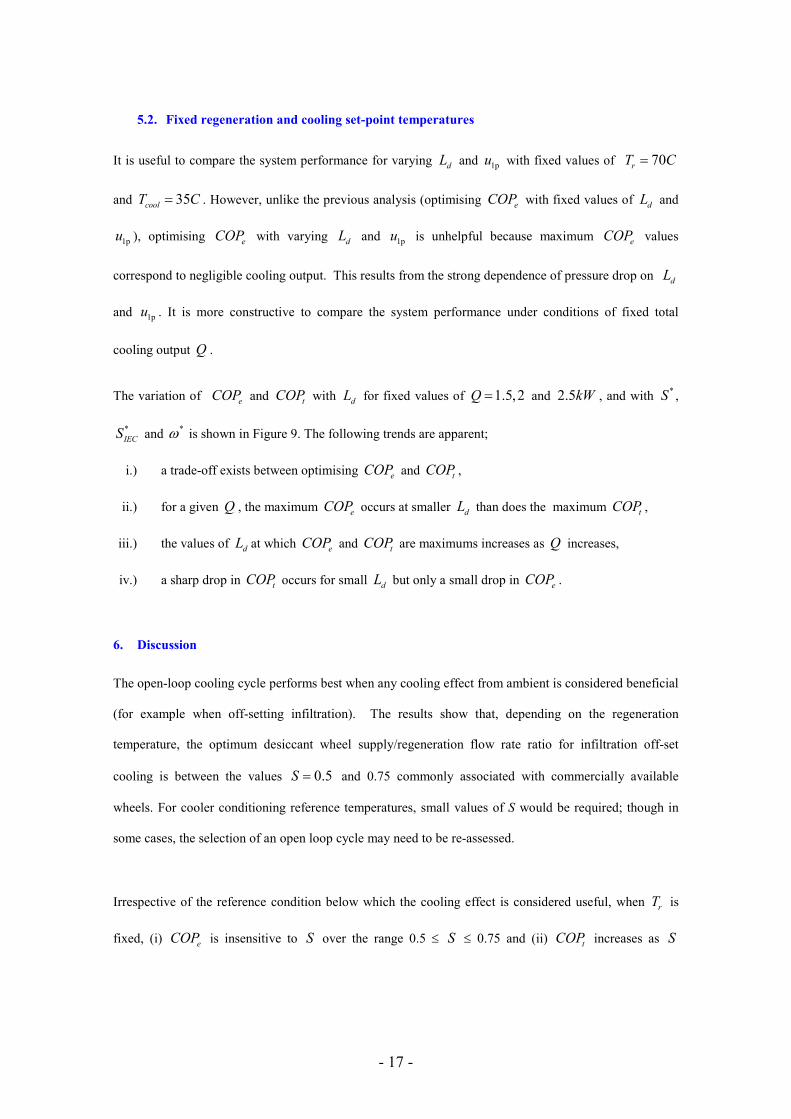
The selected cooling cycle is illustrated in Figure 1. The cycle combines a desiccant dehumidification

wheel with an indirect evaporative cooler and a heat source. A fan blows ‘supply’ air from outside

- 4 -

through the wheel (1p 2p→ ) where it is dried and slightly heated. This air then passes through the

primary channels of the indirect cooler ( 2p 3→ ) where it is sensibly cooled by heat exchange with an

evaporatively cooled air stream diverted from the main supply stream ( 3 5→ ). Depending on building

conditions, the supply air may be further cooled via a direct evaporative cooler (not shown) before it is

passed into the conditioned space.

For continuous operation, the water absorbed from the supply air must be removed from the wheel. This

is accomplished by passing a second air stream, the ‘regeneration’ air, through the wheel (1r 2r→ ),

which rotates sequentially through the dehumidification and regeneration sections. The regeneration air

stream must be hotter than the primary air stream. This can be achieved by heating the regeneration air

with a low greenhouse gas emissions heat source such as solar heat or low grade waste heat. Regeneration

air has the same humidity as the supply air as they are both sourced from ambient.

This system is similar to those proposed by other researchers (Jain and Dhar, 1996), except that there is

no heat recovery exchanger. Particularly at low regeneration temperatures, the absence of the heat

recovery heat exchanger has the potential to reduce pressure drop and associated fan electricity

consumption, without significantly reducing thermal performance.

3. Desiccant Cooling Cycle Modelling

Key design and operational variables that have potential for optimisation include;

• The fraction S of the desiccant wheel face area that is used for dehumidifying supply air. This is

typically between 0.5 and 0.75 in commercial wheels. Increasing S produces a higher flow rate of

cool air to the occupied space but leads to an increase in the humidity and temperature.

• The fraction IECS of primary air leaving the indirect evaporative cooler that is removed as a side-

stream and used to evaporatively cool the secondary side of the indirect cooler. Decreasing IECS

produces a higher flow rate of cool air but leads to an increase in the supply temperature.

- 5 -

• The wheel velocity 1pu . Increasing 1pu increases the flow-rate of supply air. However, the penalty is

an increased pressure drop, increased fan electricity consumption and increased supply air humidity

and temperature.

• The wheel length dL . Increasing dL leads to improved dehumidification and colder supply air.

However, this results in an increased pressure drop with a concomitant increase in fan electricity

consumption.

• The regeneration temperature rT . Increasing rT leads to improved dehumidification and colder

supply air. This enables the flow-rate (and thus the fan electricity consumption) to be reduced for a

given cooling load. However, the additional heating corresponds to a reduction in thermal efficiency.

• The rotational speed ω . Higher rotational speeds generally result in improved dehumidification of

the supply air but increased transfer of heat from the regeneration to supply air streams.

It is apparent that for each of these parameters, a maximum cooling effect is expected where additional

coldness is balanced by limits to either supply air flow, electricity consumption or regeneration heat

demand. A heat and mass transfer model of the complete system incorporating both the desiccant wheel

and indirect evaporative cooler has thus been constructed. The model has been used to simultaneously

optimise the cooling cycle design with respect to the parameters S , IECS , 1pu , dL , rT and ω . The

complete model incorporated two sub-models; (i) a desiccant wheel heat and mass transfer model and; (ii)

an indirect evaporative cooler heat and mass transfer model.

3.1. Desiccant wheel sub-model

A desiccant wheel consists of a large number of axis-symmetric air channels. Supply air flows through a

specified fraction of the channels and regeneration air flows counter-current in the remainder. As the

wheel rotates, the air flow through each channel cycles between the two streams. The channel walls

consist of a water adsorbent material such as silica-gel and are shaped to obtain a high surface area to

volume ratio. The desiccant material may be mechanically supported by another (non-adsorbent) material,

in which case, there is no mass transfer between channels. Typically for modelling purposes it is also

- 6 -

assumed that the channels are thermally insulated from each other and hence, that each may be considered

in isolation. Although circumferential temperature gradients occur near the supply/regeneration

changeover, this assumption is reasonable because the circumferential Fourier time for thermal diffusion

through the channel walls is small in comparison to the rotation rate. Since the channel air flows are

laminar (typically ~ 250Re ) correlations are available for transfer coefficients and hence, the air

velocity, enthalpy and moisture profiles through the channel can be approximated using cross-section

mean values. By neglecting channel curvature effects, either axial flow and lumped solid resistance (i.e.

1-D) models, or axial flow and 2-D solid diffusion models are appropriate.

3.1.1. Two dimensional desiccant wheel model formulation

A 2-D model of a desiccant channel walls is combined with a one-dimensional model of the air flow in

the channels. A sinusoidal air channel cross-section with width b and height a is assumed. The channel

length is dL and the desiccant wall (half-thickness) is c . Since c is small in comparison to the overall

radius of the wheel, radial curvature effects are ignored.

The desiccant material has a pore structure. The moisture diffusion through and along the wall is due to a

combination of (i) gas phase ordinary diffusion and (ii) Knudsen diffusion within the pores of the

desiccant and (iii) surface diffusion along the pore surfaces at desiccant/air interfaces. According to

Pesaran and Mills (1987) for regular density silica gel, the average pore radius is 11A and the ratio of gas

phase to surface diffusion is 0.023-0.06. Hence, only surface diffusion need be considered, and thus it is

approximate to consider the desiccant as a homogenous material with an overall moisture diffusivity D .

For typical wheel parameters (Table 1) 1Bi << and 1mBi > . Hence, a lumped capacitance thermal

model of the solid material in the radial direction would be appropriate. However, the slow moisture

diffusion through the desiccant limits the rate of moisture transfer between the solid and the air stream.

Consequently, a 2-D model is required to determine the moisture profile through the wall.

- 7 -

The system is modelled using moisture and energy conservation equations for the air stream moisture

content iY and temperature iT and the desiccant material moisture content W and temperature dT . The

moisture transfer between the air and the desiccant surface is proportional to the difference between the

air moisture content and the gas phase equilibrium moisture content at the surface surfY . Diffusion in the

air stream is neglected because convection is the dominant transport mechanism.

( )i i i ii surf i

i f

Y Y NTUY Y

Le

θθ

τ η∂ ∂

+ = −∂ ∂

(1)

( )i ii i i surf i

i

T TNTU T Tθ θ

τ η∂ ∂

+ = −∂ ∂

(2)

2 2

, , , ,2 2m i m i

i

W W WFo Foη κτ η κ

∂ ∂ ∂= +

∂ ∂ ∂ (3)

2 2

, ,2 2

d d di i

i

T T TFo Foη κτ η κ

∂ ∂ ∂= +

∂ ∂ ∂ (4)

where ( )2 2, 1p rS S

π πω ω

Ω = Ω = −

Equations (1)-(4) form a set of coupled parabolic partial differential equations. The desiccant is modelled

as insulated and impermeable at the channel ends and at the boundary between channels. The energy of

adsorption is assumed to be released onto the surface when moisture adsorbs onto the desiccant (also

assumed to occur at the surface). The upstream air boundary condition is specified by the inlet air

properties; the downstream air boundary conditions are extrapolated. The inflow condition and flow

direction for each channel cycles between the regeneration and supply cases according to the wheel

rotational position. The channels thus reach a cyclically steady state which is independent of the starting

conditions.

Desiccant boundary conditions:

( ) ( ) ( )

0 0

1 1

0,1 0,1

0, 0

1= ,

0 , 0

d

dm surf i surf i surf i

f pa

d

TW

TW HBi Y Y Bi T T Y Y

Le c

TW

κ κ

κ κ

η η

κ κ

κ κ

η η

= =

= =

= =

∂∂= =

∂ ∂

∂∂− = − + −

∂ ∂

∂∂= =

∂ ∂

(5)

- 8 -

Air boundary conditions:

1p

1p

1r

1r

0, for 0 1

1, for 0 1

p

p

p

r

r

r

T T

Y Y

T T

Y Y

η τ

η τ

= = < <=

= = < <

=

(6)

Non-dimensional parameters are defined as,

2

2 / 3

, , ,2 2

, , ,2 2

, =4

, ,

,

,

i i d di i a

d a pa i i

mm f

d m pa

i ii m i

d pd d d

i ii m i

d pd

u L Lh P Nu PNTU

L c A u A u

h chc hBi Bi Le Le

k fD h c

k DFo Fo

c L L

k DFo Fo

c c c

η η

κ κ

θ αρ

ρ

ρ

ρ

Ω = =

= = = =

Ω Ω= =

Ω Ω= =

(7)

Equations (1)-(4) together with the boundary conditions (Eqs. (5) and (6)) and the silica gel material and

adsorption properties (Table 1) were solved numerically using the Alternating Direct Implicit method.

Cyclical steady state conditions were assumed to exist once the total mass of water vapour entering a

channel during the supply phase was within 0.5% of the total mass leaving the channel during the

regeneration phase.

The equations were solved assuming constant adsH ,D and overall air and desiccant specific heat

capacities. These parameters were evaluated at ( )1ave 1p 1r2

T T T= + and ave 0.1W = . Sensible heat transfer

associated with the moisture transfer process was assumed to be negligible. Collectively these

assumptions were found to result in less than 1K change to the average supply side outlet temperature

and less than 10.3gkg − change in the average supply side outlet humidity compared with the exact

solution for the base case simulation.

The simulations employed constant (average) values of Nu and Sh representative of fully developed air

thermal and moisture concentration profiles throughout the channel. While larger values may be expected

- 9 -

in the entry length region, for the condition tested (1

1 / 20p du L s−> ), the influence of entry conditions is

expected to be small (Antonellis et al., 2009).

For sinusoidal channels with the specified geometry Niu and Zhang (2002) specify 2.14TNu = for the

case of constant axial surface temperature and state that typically, ~1.3H TNu Nu for the case of

constant axial surface heat flux. For the same geometry Shah (1975) gives 2.12TNu = and 2.62HNu =

although Kakac et al. (1987) specify 1.54TNu = and 2.6HNu = . Here neither the axial surface

temperature profile nor the axial surface heat flux profile were constant. Although the solid conduction

rate was high ( 1Bi << ), the insulated boundary condition employed at the internal wall acted to limit the

heat transfer rate to the desiccant (i.e. 1Foκ >> ). For the moisture transfer, the slow diffusion rate

( 1Bi > ) limited the surface moisture gradient but the axial surface moisture concentration profile was not

constant because of the coupled heat transfer. Hence, the actual values of Nu and Sh are likely to be

between TNu and HNu . Based on the more recent data, 2.4Nu = was employed here.

For the moisture transfer, Le was evaluated at aveT and the heat/mass transfer analogy employed to

calculate Sh . Since 1Le < , the mass transfer across the desiccant surface is enhanced relative to the

energy transfer. The influence of varying Le has been investigated by Van den Bulck et al. (1985).

However, in their model, the effect of solid side diffusion was included in the definition of Le , and this

led to 1Le > . Often it may be appropriate to assume that 1Le = . This assumption does not significantly

change the predicted values of 2pY and 2pT .

3.1.2. Desiccant wheel model validation

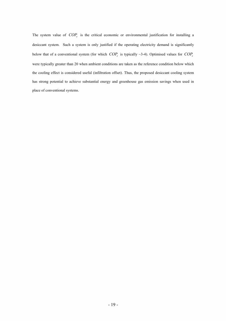
Validation of the wheel model was achieved by comparing the predicted average supply outlet condition

with experimental data (Tsutsui et al., 2008) for varying ω and dL for set inlet conditions. The

parameters and conditions used are listed in Table 1. Simulation results are shown in Figure 2; dots

represent the experimental values and solid lines the simulation results. It is evident that the simulation

- 10 -

model can predict the variations of average supply outlet temperature 2pT and humidity ratio 2pY with ω

and dL over a reasonable range of these parameters. Generally, the simulation 2pT values are lower than

the experimental values by approximately 2K and the agreement is closer for lower rotation speeds.

3.2. Indirect evaporative cooler sub-model

An indirect evaporative cooler, consists of a series of alternating dry and wet flow channels. In the dry

channels, ‘primary’ air stream is cooled sensibly via heat transfer with a ‘secondary’ air stream in the wet

channels. In the wet channels a flow of water along the walls evaporatively cools the secondary air

stream. Multiple geometric flow-arrangements are possible including, parallel, cross and counter-current

flow. For given conditions, the cooling performance may be expressed using the effectiveness defined by

2p 3

2p _3wb

T T

T Tε

−=

−. (8)

Note that the denominator in Eq. (8) contains the primary channel exit wet bulb temperature. That is, the

maximum effectiveness of 1 is obtained when the inlet air is cooled to its dew point temperature.

A cross flow indirect cooler design is described by Pescod (1974). The water flow in the wet air channel

is in the downwards direction opposite to the secondary air flow. Both the wet and dry channels have

protrusions spaced at regular intervals to improve the heat transfer by promoting turbulent flow in the

channels, even though this also increases the air-flow pressure drops. The key design parameters are the

channel spacings, protrusion details, channel lengths, air and water flow-rates and flow velocities.

The performance of a cross-flow regenerative indirect cooler has been analysed numerically by Erens and

Dreyer (1993). For a given inlet design temperature and humidity ratio, they present a graph of the

cooling capacity as a function of IECS for a range of plate spacings, assuming equal spacing for the dry

and wet channels. The optimum value of IECS was found to be between 0.25 and 0.4 for plate spacings

between 2 and 5mm. This corresponds to secondary stream flow rates significantly below those leading to

the maximum effectiveness (for which ~1IECS ) .

- 11 -

Previous numerical and experimental studies of indirect cooler performance have considered inlet flow

conditions representative of ambient summer cooling conditions. However, in this case, the primary air

stream is sourced from the outlet of the desiccant wheel. These inlet conditions are likely to be

significantly hotter and dryer than that used in previous studies. Thus, a 2-D heat and mass transfer model

of the indirect cooler has been used to estimate the variation in ε over a range of inlet conditions and

IECS for a cross-flow regenerative cooler.

3.2.1. Two dimensional indirect evaporative cooler model formulation

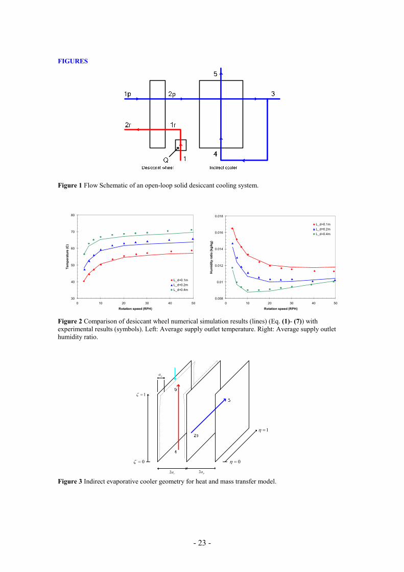
The indirect cooler is shown schematically in Figure 3. Primary air flows through the right (dry) channel

from the inlet at ‘2p’ to the outlet at ‘3’. A portion of the air at ‘3’ is diverted to the left (wet) channel and

passes from ‘4’ to ‘5’. A water film with thickness wa runs down the side of the wet channel from ‘5’ to

‘4’. The dry channel and wet channels have thicknesses of 2 pa and 2 sa respectively.

Because the thermal resistance of the channel walls is small (the Fourier heat transfer time is large), it is

appropriate to assume that the wall and water film temperatures are identical at a given location.

According to Madhawa et al. (2007), the influence on ε of conduction in the plane of the water/wall

surface is small (<5%) for most conditions. Here all conduction effects are neglected.

Assuming that the variation in wa is small, the following five equations may be formulated expressing

conservation of energy and mass of the primary and secondary air streams and the water flow at the

steady state condition. Here satY is the saturated air moisture content at the local water temperature wT ,

,p pT Y are the primary channel air temperature and humidity ratio and ,s sT Y the secondary channel air

temperature and humidity ratio. The wetability factor ψ is an adjustable parameter to account for

incomplete wetting of the plate surface by the water film.

- 12 -

( )p

p w p

TNTU T T

η

∂= − −

∂ (9)

0pY

η

∂=

∂ (10)

( ) ( )sat

1 vapss w s s

f pa

HTNTU T T Y Y

Le cψ

ζ

∂= − − + −

∂ (11)

( )sats s

s

f

Y NTUY Y

Leψ

ζ∂

= − −∂

(12)

( ) ( )pa pws w s w p

pw IEC

c NTUTNTU T T T T

c Sβ

ζ ∂

= − + − ∂ (13)

Equations (9)-(13) form a coupled set of differential equations. For regenerative operation with a closed

loop water cycle, only the inlet temperature 2pT and humidity ratio 2pY of the primary stream and the inlet

water temperature must be specified. Here the water inflow condition employed is equivalent to an

external reservoir which is small in comparison to the water circulation rate and which rapidly reaches the

temperature of the water exiting the flow channels. The resultant boundary conditions are:

( ) ( )

( ) ( ) ( ) ( )

( ) ( )

2p 2p, 0 , , 0

0, , 1 , 0, , 1

1, 0,

p p

s p s p

w w

T T Y Y

T T Y Y

T T

ζ η ζ η

ζ η ζ η ζ η ζ η

ζ η ζ η

= = = =

= = = = = =

= = =

(14)

Non-dimensional parameters are defined as:

2p 4

1 1, , ,

p s s sp s IEC

a pa p a pa s w p

h h m mL HNTU NTU S

c a u c a u m mβ

ρ ρ= = = =

ɺ ɺ

ɺ ɺ (15)

Here it has been assumed that the total air specific heat capacity is constant, that negligible sensible heat

transfer is combined with the moisture transfer and, that the variation in wa is small. Collectively these

assumptions were found to result in less than a 2% change in ε compared with the exact solution for the

base case simulation conditions listed in Table 2.

- 13 -

The performance of the indirect evaporative cooler, measured in terms of ε as defined in Eq. (8), is

highly dependent on the heat transfer coefficients in the dry and wet channels ph and sh . Here a

correlation of the form bh Au= (Pescod, 1979) was employed with parameters as given in Table 2.

3.2.2. Indirect evaporative cooler model validation

Validation of the indirect evaporative cooler model was achieved by comparing the predicted

effectiveness values with experimental data (White et al., 2009) for primary air inlet temperatures

( 2p 303,323T K= ), humidities (1

2p 5,10,15Y gkg −= ) and mass flow ratios ( 0.4,0.6IECS = ). Other

parameters and conditions used are listed in Table 2 and comparisons between calculated and

experimental results are illustrated in Figure 5.

The large uncertainty range associated with the experimental values is due to the high number of sensors

from which data was recorded to determine the cross-sectional averaged properties. The model

predictions are largely within the range of experimental error, though the predicted values for ε only

approximately match the experimental results over the full range of conditions. In particular, the

experimental results indicate a drop in performance at high inlet humidity levels. However, the presence

of the desiccant wheel upstream of the indirect cooler in the system simulations insured that the 15g/kg

humidity level was not reached in subsequent desiccant cycle simulations.

3.3. Desiccant cycle optimisation

The two sub-models were combined into a single open-loop cooling model with the addition of an

optimisation routine used to; (i) calculate and maximise the electrical coefficient of performance eCOP

and; (ii) calculate and report the thermal coefficient of performance tCOP . The eCOP was defined as the

ratio of useful cooling to parasitic fan electricity consumption (Eq. (16)) and tCOP as the ratio of useful

cooling to regeneration heat consumption (Eq. (17)).

- 14 -

( )( )( )

1p 2p 2p 3 1p

1p 2p 2p 3 4 5

1a cool

e IEC

H H HCOP S S

P P P

ρφ → → →

→ → →

∆ + ∆ − ∆= −

∆ + ∆ + ∆ (16)

( )( )

( )1p 2p 2p 3 1p1p

1r 1 1r

1

1

coolIEC

t

H H Hu S SCOP

u S H

→ → →

→

∆ + ∆ − ∆−=

− ∆, (17)

Here H∆ is the enthalpy change between the given state points. The useful cooling effect (numerator)

depends on the reference condition below which the cooling effect is considered to be useful. In some

cases, any enthalpy removal below the ambient (outside) condition is useful (for example for

displacement of ventilation air). In other cases, it is only the enthalpy reduction below the indoor

condition that is useful. Additional flexibility was provided in the model by allowing the user to set their

preferred reference condition coolT and coolY below which useful cooling is obtained.

In Eq. (16) the fan electricity consumption (denominator) is calculated from (i) the fan efficiency and (ii)

the summed pressure drop across both the primary air flow path (desiccant wheel and indirect cooler

primary air channels) and the secondary air flow path of the indirect cooler. This assumes that

• the pressure drop across the supply and regeneration sides of the wheel are equal;

• the pressure drop along the building supply air ductwork matches the pressure drop across

the secondary side of the indirect cooler.

The pressure drops across each of the components were calculated using Eqs. (18)-(20), and the fan

electrical efficiency φ was set to 0.8 for all calculations.

2

2

1p 2p 1 1p 1p 1p 2p

1

32 2

d ad a

f PP F u L u K

A

µρ→ →

∆ = +

, 1

1.65F = (18)

2

2p 3 2 2p 2p 2p 32

1 1

32 2

IEC aa

p

fP F u L u K

a

µρ→ →

∆ = +

,

21.5F = (19)

2

4 5 3 4 4 4 52

1 1

32 2

IEC aa

s

fP F u H u K

a

µρ→ →

∆ = +

,

33.5F = (20)

Here 1 2p pK → is the minor loss coefficient for the desiccant channels. For the (laminar flow) desiccant

channels, the variation in pressure drop with channel velocity is close to linear over a range of typical

velocities since df is constant and the contribution of minor losses is relatively small. For the indirect

- 15 -

cooler, the methodology of Pescod (1979) was employed to express the pressure drop in the turbulent

channels as the combination of a friction effect between the protrusions, the drag induced pressure drop

due to the protrusions and that due to minor (entrance and exit) losses. Scaling factors 1 2 3, ,F F F were

introduced to match the theoretical expressions with experimental measurements (White et al., 2009). The

particularly large value of 3F arises because the theoretical expression ignored the pressure drop due to

passage of air through the demister pad located at the secondary air stream exit. Predicted and

experimental pressure drops are compared for an indirect cooler and an equivalent geometry silica-gel

desiccant wheel (Rossington et al., 2009), as functions of the stream inlet face velocity, in

Figure 5.

4. Procedure

The performance of the desiccant cooling system is a function of a large number of parameters. Here the

system performance was optimised by varying the parameters,

1p, , , , ,IEC r dS S T L uω

with fixed values of the following parameters with values as listed in Table 1 and Table 2.

1r 1p, , , , , , ,

, , , , , , ,

Pd pd d A

p s p s

c k D c Nu u u

L H a a h h

ρ

ψ β

=.

Because the dimensions of the indirect cooler were fixed, the face area of the wheel was set to a constant

value of 20.196m . This is equivalent to setting the scaling between the wheel and indirect cooler face

velocities.

In the following text, the optimum parameter values are indicated using a superscript ‘*’. The optimum

value of ω , (i.e. *ω ) was chosen as that leading to maximum dehumidification at the desiccant supply

side outlet. For all other parameters, eCOP was used as the optimisation criterion. The results are

presented in two parts.

- 16 -

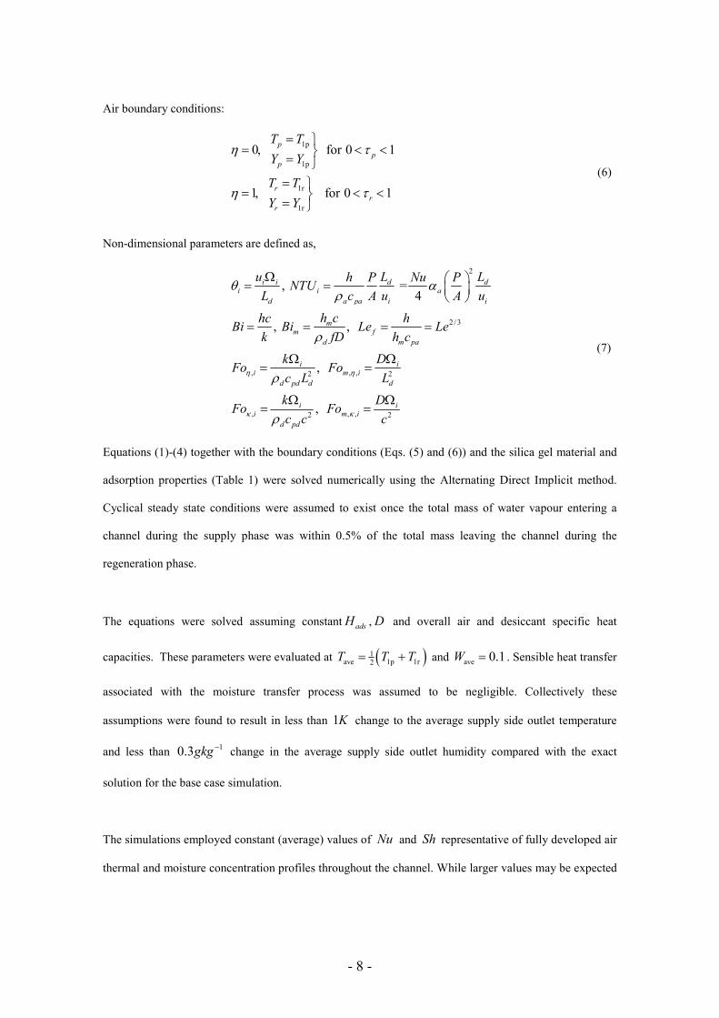
1. In Section 5.1 a fixed value of dL and 1pu is considered and *ω ,

*S and *

IECS calculated for

50 80rC T C≤ ≤ and 24 35coolC T C≤ ≤ with 114.3coolY gkg −= .

2. In Section 5.2, a varying wheel length 0.05 0.4dL≤ ≤ and inlet channel velocity was

considered and *ω ,

*S and *

IECS calculated for 70rT C= and 35coolT C= with

114.3coolY gkg −= .

In all cases, a fixed inlet (ambient) condition of 1p 35T C= and 1

1p 14.3HR gkg −= was employed.

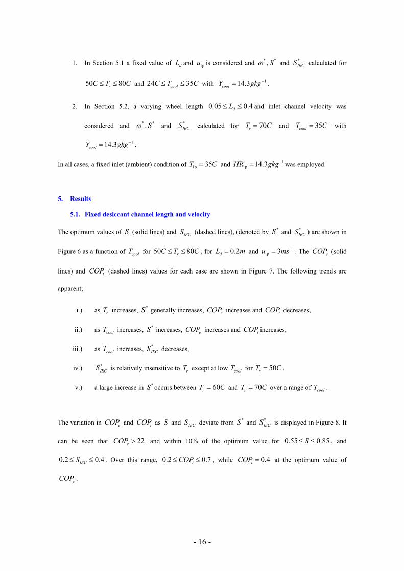
5. Results

5.1. Fixed desiccant channel length and velocity

The optimum values of S (solid lines) and IECS (dashed lines), (denoted by *S and

*

IECS ) are shown in

Figure 6 as a function of coolT for 50 80rC T C≤ ≤ , for 0.2dL m= and 1

1p 3u ms−= . The eCOP (solid

lines) and tCOP (dashed lines) values for each case are shown in Figure 7. The following trends are

apparent;

i.) as rT increases, *S generally increases, eCOP increases and tCOP decreases,

ii.) as coolT increases, *S increases, eCOP increases and tCOP increases,

iii.) as coolT increases, *

IECS decreases,

iv.) *

IECS is relatively insensitive to rT except at low coolT for 50rT C= ,

v.) a large increase in *S occurs between 60rT C= and 70rT C= over a range of coolT .

The variation in eCOP and tCOP as S and IECS deviate from *S and

*

IECS is displayed in Figure 8. It

can be seen that 22eCOP > and within 10% of the optimum value for 0.55 0.85S≤ ≤ , and

0.2 0.4IECS≤ ≤ . Over this range, 0.2 0.7tCOP≤ ≤ , while 0.4tCOP = at the optimum value of

eCOP .

- 17 -

5.2. Fixed regeneration and cooling set-point temperatures

It is useful to compare the system performance for varying dL and 1pu with fixed values of 70rT C=

and 35coolT C= . However, unlike the previous analysis (optimising eCOP with fixed values of dL and

1pu ), optimising eCOP with varying dL and 1pu is unhelpful because maximum eCOP values

correspond to negligible cooling output. This results from the strong dependence of pressure drop on dL

and 1pu . It is more constructive to compare the system performance under conditions of fixed total

cooling output Q .

The variation of eCOP and tCOP with dL for fixed values of 1.5,2Q = and 2.5kW , and with *S ,

*

IECS and *ω is shown in Figure 9. The following trends are apparent;

i.) a trade-off exists between optimising eCOP and tCOP ,

ii.) for a given Q , the maximum eCOP occurs at smaller dL than does the maximum tCOP ,

iii.) the values of dL at which eCOP and tCOP are maximums increases as Q increases,

iv.) a sharp drop in tCOP occurs for small dL but only a small drop in eCOP .

6. Discussion

The open-loop cooling cycle performs best when any cooling effect from ambient is considered beneficial

(for example when off-setting infiltration). The results show that, depending on the regeneration

temperature, the optimum desiccant wheel supply/regeneration flow rate ratio for infiltration off-set

cooling is between the values 0.5S = and 0.75 commonly associated with commercially available

wheels. For cooler conditioning reference temperatures, small values of S would be required; though in

some cases, the selection of an open loop cycle may need to be re-assessed.

Irrespective of the reference condition below which the cooling effect is considered useful, when rT is

fixed, (i) eCOP is insensitive to S over the range 0.5 ≤ S ≤ 0.75 and (ii) tCOP increases as S

- 18 -

increases. This indicates that a small drop in eCOP may be permitted via selection of S slightly larger

than *S to obtain a significant improvement in tCOP .

The system performance was slightly more sensitive to IECS for fixed rT . The optimum range occurred

over relatively low ratios; between * 0.3 0.4IECS = − for the high flow, infiltration offset case and

increasing to * 0.5IECS = for cooler reference conditions.

The values of *S and

*

IECS predicted in the desiccant wheel study of Chung and Lee (2009) and in the

indirect cooler study of Erens and Dreyer (1993) were * 0.6S ≈ at 80rT C= and

* 0.25 0.4IECS ≈ − (for

4mm to 2mm channel spacings) respectively. The similarity with this study is interesting given that these

studies (i) considered a single component in isolation, and (ii) employed different parameters and

performance indicators (the moisture removal capacity and total cooling power) to those used here. In

both cases the performance was evaluated using a reference condition equal to the inlet (i.e. ambient)

condition for the component. The similarity suggests that in general, the values predicted here may be

approximately correct for a number of systems.

Use of eCOP and tCOP as performance indicators highlights the trade-off which exists, particularly in

solar applications, between minimising the operating costs and minimizing the capital cost. By employing

an increased collector area, or higher operating temperature collectors, the regeneration temperature can

in turn be increased. This increases eCOP (the operating cost indicator) but lowers tCOP (the capital

cost indicator).

This trade-off is also evident in the comparison of varying desiccant wheel lengths and inlet velocities.

The optimum length of the wheel for maximising eCOP , is significantly shorter than the optimum length

for maximising tCOP . Clearly, the performance of solar air-conditioning systems should be presented in

terms of both eCOP and tCOP .

- 19 -

The system value of eCOP is the critical economic or environmental justification for installing a

desiccant system. Such a system is only justified if the operating electricity demand is significantly

below that of a conventional system (for which eCOP is typically ~3-4). Optimised values for eCOP

were typically greater than 20 when ambient conditions are taken as the reference condition below which

the cooling effect is considered useful (infiltration offset). Thus, the proposed desiccant cooling system

has strong potential to achieve substantial energy and greenhouse gas emission savings when used in

place of conventional systems.

- 20 -

REFERENCES

1. Antonellis, S., Joppolo, C. and Molinaroli, L. Desiccant wheels models: investigation on the

fully developed temperature and velocity profile assumption in 3rd International Solar Air-

conditioning conference. 2009. Palermo: OTTI.

2. Brandermuehl, M., Analysis of heat and mass transfer regenerators with time varying or

spatially nonuniform inlet conditions, Ph.D thesis, in University of Wisconsin. 1982: Madison.

3. Charoensupaya, D. and W. Worek, Effect of adsorbent heat and mass transfer resistances on

performance of an open-cycle adiabatic desiccant cooling system. Heat recovery systems and

CHP, 1988. 8(6): p. 537-548.

4. Chung, J. and D. Lee, Effect of desiccant isotherm on the performance of desiccant wheel.

Journal of refrigeration, 2009. 32: p. 720-726.

5. CRC Handbook of Chemistry and Physics, 89th Edition (Internet Version 2009), ed. D.R. Lide.

2009, Boca Raton, FL: CRC Press/Taylor and Francis.

6. Erens, P. and A. Dreyer, Modelling of indirect evaporative air coolers. International journal of

heat and mass transfer, 1993. 36(1): p. 17-26.

7. Ge, T., et al., A review of the mathematical models for predicting rotary desiccant wheel.

Renewable and sustainable energy reviews, 2008. 12: p. 1485-1528.

8. Incropera, F. and D. DeWitt, Fundamentals of Heat and Mass Transfer. 2002, New Jersey:

Wiley.

9. Jain, S. and P. Dhar, Evaluation of solar-desiccant-based evaporative cooling cycles for typical

hot and humid climates. Fuel and energy abstracts, 1996. 37(1): p. 286-296.

10. Kakac, S., R. Shah, and W. Aung, Handbook of single-phase convective heat transfer. 1987,

New York: Wiley.

11. Maclaine-cross, I. and P. Banks, Coupled heat and mass transfer in regenerators - prediction

using an analogy with heat transfer. International journal of heat and mass transfer, 1972. 15: p.

1225-1242.

12. Maclaine-cross, I. and P. Banks, A general theory of wet surface heat exchangers and its

application to regenerative evaporative cooling. Journal of heat transfer, 1983. 103: p. 579-585.

- 21 -

13. Madhawa, H., M. Golubovic, and W. Worek, The effect of longitudinal heat conduction in cross

flow indirect evaporative air coolers. Applied thermal engineering, 2007. 27: p. 1841-1848.

14. Ng, K., et al., Experimental investigation of the silica gel-water adsorption isotherm

characteristics. Applied thermal engineering, 2001. 21: p. 1631-1642.

15. Niu, J. and L. Zhang, Heat transfer and friction coefficients in corrugated ducts confined by

sinusoidal and arc curves. International journal of heat and mass transfer, 2002. 45: p. 571-578.

16. Ouazia, B., et al., Desiccant-evaporative cooling system for residential buildings, in 12th

Canadian Conference on Building Science and Technology. 2009, NRC: Montreal.

17. Pesaran, A. and A. Mills, Moisture transport in silica gel packed bed. I Theoretical study.

International journal of heat and mass transfer, 1987. 30(6): p. 1037-1049.

18. Pescod, D., An evaporative air cooler using a plate heat exchanger. 1974, CSIRO: Highett.

19. Pescod, D., A heat exchanger for energy saving in an air-conditioning plant. ASHRAE

Transactions, 1979. 85(2): p. 238-251.

20. Rossington, D., et al. Comparison of silica gel and zeolite desiccant wheel performance. in 3rd

International Solar Air-conditioning conference 2009. Palermo: OTTI.

21. Shah, R., Laminar flow friction and forced convection heat transfer in ducts of arbitrary

geometry. International journal of heat and mass transfer, 1975. 18: p. 849-862.

22. Smith, R., C. Hwang, and R. Dougall, Modelling of a solar-assisted desiccant air conditioner for

a residential building. Energy, 1993. 19(6): p. 679-691.

23. Sladek, K., E. Gilliland, and R. Baddour, Diffusion on surface II. Correlation of diffusivities of

physically and chemically adsorbed species. Ind. Eng. Chem. Fundamentals, 1974. 13(2): p.

100-105.

24. Stabat, P. and D. Marchio, Heat and mass transfers modelled for rotary desiccant dehumidifiers.

Applied energy, 2008. 85: p. 128-142.

25. Thur, A. and M. Vukits. Solar heating and cooling - town hall Gleisdorf in 3rd International

Solar Air-conditioning conference. 2009. Palermo: OTTI.

26. Tsutsui, K., et al., Effect of design and operating conditions on performance of desiccant wheels,

in 2008 HVAC energy efficiency best practice conference. 2008, AIRAH: Melbourne.

- 22 -

27. Van den Bulck, E., J. Mitchell, and S. Klein, Design theory for rotary heat and mass exchangers

-II. Effectiveness -number of transfer units method for rotary heat and mass exchangers

International journal of heat and mass transfer, 1985. 28(8): p. 1587-1595.

28. White, S., P. Kohlenbach, and C. Bongs, Indoor temperature variations resulting from solar

desiccant cooling in a building without thermal backup. International Journal of Refrigeration,

2009. 32: p. 695-704.

29. White, S., Rossington, D., Goldsworthy, M., Reece, R. and Sire, R., Experimental performance

characterisation of an indirect evaporative cooler. 2009, Newcastle: CSIRO.

- 23 -

FIGURES

Figure 1 Flow Schematic of an open-loop solid desiccant cooling system.

30

40

50

60

70

80

0 10 20 30 40 50

Rotation speed (RPH)

Temperature (C)

L_d=0.1m

L_d=0.2m

L_d=0.4m

0.008

0.01

0.012

0.014

0.016

0.018

0 10 20 30 40 50

Rotation speed (RPH)

Humidity ratio (kg/kg)

L_d=0.1m

L_d=0.2m

L_d=0.4m

Figure 2 Comparison of desiccant wheel numerical simulation results (lines) (Eq. (1)- (7)) with

experimental results (symbols). Left: Average supply outlet temperature. Right: Average supply outlet

humidity ratio.

2s

a 2p

a

wa

0η =

1η =

0ζ =

1ζ =

Figure 3 Indirect evaporative cooler geometry for heat and mass transfer model.

- 24 -

0.2

0.3

0.4

0.5

0.6

0.7

10 15 20 25 30 35 40

Twb_2p

Effectiveness

Exp. T_2p=30C, S_IEC=0.6

Model T_2p=30C S_IEC=0.6

Exp. T_2p=50C, S_IEC=0.6

Model T_2p=50C, S_IEC=0.6

Exp. T_2p=30C, S_IEC=0.4

Model T_2p=30C, S_IEC=0.4

Exp. T_2p=50C, S_IEC=0.4

Model T_2p=50C, S_IEC=0.4

Figure 4 Comparison of indirect evaporative cooler numerical simulation results (lines) (Eq.(9) - (15))

with experimental results (symbols) for conditions and with parameters as listed in

Table 1.

0

50

100

150

200

250

0.0 0.5 1.0 1.5 2.0 2.5

Face velocity (m/s)

dP (Pa)

Exp. data dP_p

Exp. data dP_s

Eq. 19

Eq. 20

0

50

100

150

200

250

300

350

400

0.0 0.5 1.0 1.5 2.0 2.5 3.0 3.5 4.0

Face velocity (m/s)

dP (Pa)

Exp. data

Eq. 18

Figure 5 Left: Indirect cooler pressure drops as a function of channel entrance face velocity.

Experimental data (White et al., 2009) and Eqs. (19) and (20). Right: Desiccant wheel pressure drop as a

function of face velocity. Experimental data (Rossington et al., 2009) and Eq. (18).

0.3

0.35

0.4

0.45

0.5

0.55

0.6

0.65

0.7

22 24 26 28 30 32 34 36

T_cool (C)

S*

0.2

0.3

0.4

0.5

0.6

0.7

S_IEC*

S

S_IEC

80C

80C

50C

50C

Figure 6 Variation of optimum desiccant wheel ratio *S (solid lines) and indirect cooler ratio *

IECS (dashed

lines) with cooling set-point temperature coolT for different desiccant regeneration temperatures

rT .

- 25 -

0

10

20

30

22 24 26 28 30 32 34 36 38

T_cool (C)

COP_e

0

0.2

0.4

0.6

0.8

1

COP_t

COP_e

COP_t

50C

80C

80C

Figure 7 Comparison of

eCOP (solid lines) and tCOP (dashed lines) for varying values of

rT and cooling

set-point temperature coolT with optimum system parameters for each condition.

5

5

55

5

10

10

10

10

10

15

15

15

15

15

20

20

20

20

20

21

21

21

21

21

22

22

22

22

23

23

23

24

24

SP

SIEC

r

0.1 0.2 0.3 0.4 0.5 0.6 0.7 0.8 0.90.1

0.2

0.3

0.4

0.5

0.6

0.7

0.8

0.9

0.1

0.1

0.1

0.1

0.2

0.2

0.2

0.2

0.30.3

0.3

0.4

0.4

0.4

0.5

0.5

0.5

0.6

0.6

0.7

0.7 0.8

0.8

0.9

1

SP

SIEC

Tr=70C

0.1 0.2 0.3 0.4 0.5 0.6 0.7 0.8 0.90.1

0.2

0.3

0.4

0.5

0.6

0.7

0.8

0.9

Figure 8 Contours of

eCOP (left) and tCOP (right) for varying S and

IECS with 70rT C= and 35coolT C= .

0.05 0.1 0.15 0.2 0.25 0.3 0.35 0.40

10

20

30

40

50

60

70

Ld

COPe

0.2

0.25

0.3

0.35

0.4

0.45

0.5

0.15

COPt

COPe

COPt

Q=2kW

Q=2.5kW

Q=1.5kW

Figure 9 Plot of

eCOP (solid lines) and tCOP (dashed lines) for constant values of the total cooling output

Q as a function of dL for 70rT C= and 35coolT C= with *S , *

IECS and *ω .

- 26 -

TABLES

Wheel material properties Wheel conditions Non-dimensional data

0.7f =

1 1

3

1 1

921

800

0.2

pd

d

d

c Jkg K

kgm

k Wm K

ρ

− −

−

− −

=

=

=

(Ng et al., 2001)

44.7df = (Niu and Zhang, 2002)

1p

1r

1

1p

1

1r

1

1p 1r

305.5

353.2

19.5

11.9

3 50

0.5

2.86

T K

T K

Y gkg

Y gkg

RPH

S

u u ms

ω

−

−

−

=

=

=

=

= −

=

= =

Re 242, 2.4Nu= =

0.87Le = (CRC, 2009)

4

3

6

,

,

7.47

1287

0.028, 10.0

6.1 10

1.6 10

1.6 10

4.0

m

m

m

NTU

Bi Bi

Fo

Fo

Fo

Fo

κ

κ

η

η

θ

−

−

=

=

= =

= ×

= ×

= ×

=

Wheel construction

( )0.622 3816.44

, exp 23.196/ 46.13

surf s

atm s surf

Y PP P T

ϕϕ

= = − − −

2 3 40.0078 0.0576 24.17 124.48 204.23

surf surf surf surfW W W Wϕ = − + − +

(Pesaran, 1987)

( )1 0.2843exp 10.28ads vap surfH H W = + − (Brandermuehl, 1982)

6 2exp 0.45 , 1.6 10 /ads

o o

surf

HD D D m s

RT

−

= − = ×

(Sladek et al., 1974)

3.8

1.9

0.125

a mm

b mm

c mm

=

=

=

1

0.1 0.4

0.7

/ 2664

dL m

P A m

ν−

= −

=

=

Table 1 Desiccant wheel properties, validation conditions and ‘base’ case parameters.

Indirect cooler

conditions

Indirect cooler

construction

Material data Non-dimensional

data

2p

1

2p

1

2p

1

4

303 323

5 15

2.9 3

2.9 4.5

T K

Y gkg

u ms

u ms

−

−

−

= −

= −

= −

= −

10.003

wm Ls

per channel

−=ɺ

0.37

0.55

3.5

2

p

s

L m

H m

a mm

a mm

=

=

=

=

0.6 2 132 h u Wm K− −=

( )s wY T

( )vap wH T

96IECf = (Incropera, 2002)

237

1

pRe

Le

=

=

3.20,3.24

0.4,0.6

1.35,2.1

0.3

p

IEC

NTU

S

βψ

=

=

=

=

Table 2 Indirect cooler parameters and validation conditions.