Page 1
OPTIMISATION OF SOLID-STATE AND SOLUTION-BASED SERS
SYSTEMS FOR USE IN THE DETECTION OF ANALYTES OF CHEMICAL
AND BIOLOGICAL SIGNIFICANCE
A thesis submitted to The University of Manchester for the degree of Doctor of
Philosophy in the Faculty of Engineering and Physical Sciences
2012
Samuel Bernard Mabbott
School of Chemistry
Page 2
2
Contents List of Tables..................................................................................................................... 5
List of Figures ................................................................................................................... 7
List of Schemes ............................................................................................................... 11
Abstract ........................................................................................................................... 12
Declaration ...................................................................................................................... 13
Copyright Statement ....................................................................................................... 14
Abbreviations .................................................................................................................. 15
Acknowledgements ......................................................................................................... 16
1. Introduction ............................................................................................................. 17
1.1 The Electromagnetic Spectrum and its Wave/Particle Duality Relationship ....... 18
1.2 Radiation and Analyte Interactions ....................................................................... 22
1.3 Theory of the Raman Effect .................................................................................. 25
1.4 Raman Instrumentation ......................................................................................... 33
1.5 Alternative Methods of Raman Spectroscopy....................................................... 36
1.6 Non-Instrumentational Techniques ....................................................................... 39
1.7 Surface enhanced Raman spectroscopy (SERS) ................................................... 40
1.8 Mechanisms of SERS ............................................................................................ 42
1.9 Nanoparticles and SERS Substrates ...................................................................... 45
1.10 Aims and Objectives ........................................................................................... 47
1.11 References ........................................................................................................... 48
2. Preliminary Work on the Synthesis of Solid-State SERS Active Substrates .............. 51
2.1 Abstract ................................................................................................................. 52
2.2 Introduction - Setting the Scene for Successful Solid-State SERS Substrate
Synthesis ..................................................................................................................... 53
2.3 Preliminary synthesis 1 – Nanoparticle Substrates ............................................... 54
2.3.1 Materials ......................................................................................................... 54
2.3.2 Methods .......................................................................................................... 54
2.3.3 Results and Discussion ................................................................................... 59
2.4 Preliminary Synthesis 2 –Silver Nanoclusters deposited on Aluminium Foil ...... 66
2.4.1 Materials ......................................................................................................... 66
2.4.2 Methods .......................................................................................................... 66
2.4.3 Results and Discussion ................................................................................... 67
2.5 Conclusion ............................................................................................................ 69
2.6 References ............................................................................................................. 70
3. The Optimisation of Facile Substrates for Surface Enhanced Raman Scattering
through Galvanic Replacement of Silver onto Copper. .................................................. 71
Page 3
3
3.1 Abstract ................................................................................................................. 72
3.2 Introduction ........................................................................................................... 73
3.3 Experimental ......................................................................................................... 76
3.3.1 Materials ......................................................................................................... 76
3.3.2 Methods .......................................................................................................... 76
3.4 Results and Discussion .......................................................................................... 80
3.5 Conclusion ............................................................................................................ 97
3.6 References ............................................................................................................. 98
4. The Assessment of the Reproducibility of the Silver on Copper (SoC) SERS
Substrate and Performance Comparison with Commercially Available Substrates;
Klarite and QSERS. ...................................................................................................... 100
4.1 Abstract ............................................................................................................... 101
4.2 Introduction ......................................................................................................... 102
4.3 Experimental ....................................................................................................... 104
4.3.1 Materials ....................................................................................................... 104
4.3.2 Methods ........................................................................................................ 105
4.4 Results and Discussion ........................................................................................ 107
4.5 Conclusion .......................................................................................................... 128
4.6 References ........................................................................................................... 130
5. 2p or not 2p: Tuppence-based SERS for the Detection of Illicit Materials. ............. 132
5.1 Abstract ............................................................................................................... 133
5.2 Introduction ......................................................................................................... 134
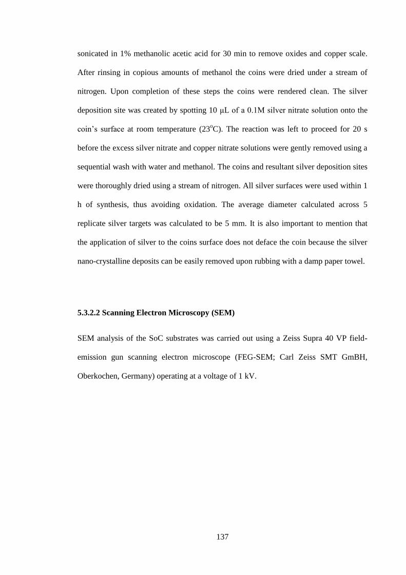
5.3 Experimental ....................................................................................................... 136
5.3.1 Materials ....................................................................................................... 136
5.3.2 Methods ........................................................................................................ 136
5.4 Results and Discussion ........................................................................................ 140
5.5 Conclusion .......................................................................................................... 144
5.6 References ........................................................................................................... 145
6. Application of Surface Enhanced Raman Scattering to the Solution Based Detection
of a Popular Legal High, 5,6-methylenedioxy-2-aminoindane (MDAI) ...................... 146
6.1 Abstract ............................................................................................................... 147
6.2 Introduction ......................................................................................................... 148
6.3 Experimental ....................................................................................................... 151
6.3.1 Materials ....................................................................................................... 151
6.3.2 Methods ........................................................................................................ 151
6.4 Results and Discussion ........................................................................................ 156
6.5 Conclusion .......................................................................................................... 164
6.6 References ........................................................................................................... 165
Page 4
4
7. The Optimisation of Parameters for the Quantitative Surface Enhanced Raman
Scattering (SERS) Detection of Mephedrone using a Fractional Factorial Design and a
Portable Raman Spectrometer ....................................................................................... 167
7.1 Abstract ............................................................................................................... 168
7.2 Introduction ......................................................................................................... 169
7.3 Experimental ....................................................................................................... 172
7.3.1 Materials ....................................................................................................... 172
7.3.2 Methods ........................................................................................................ 172
7.4 Results and Discussion ........................................................................................ 176
7.5 Conclusion .......................................................................................................... 188
7.6 References ........................................................................................................... 189
8. The Discrimination of Antibiotics and in-situ Analysis of β-Lactam Hydrolysis of
Ampicillin using Surface Enhanced Raman Scattering ................................................ 192
8.1 Abstract ............................................................................................................... 193
8.2 Introduction ......................................................................................................... 194
8.3 Experimental ....................................................................................................... 197
8.3.1 Materials ....................................................................................................... 197
8.3.2 Methods ........................................................................................................ 197
8.4 Results and Discussion ........................................................................................ 201
8.5 Conclusion .......................................................................................................... 214
8.6 References ........................................................................................................... 216
9 Conclusions and Future Work .................................................................................... 218
10 Appendix .................................................................................................................. 224
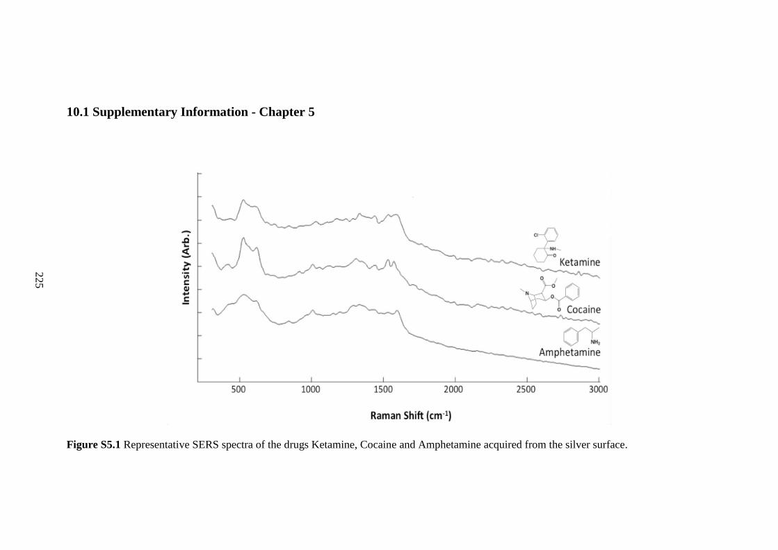
10.1 Supplementary Information - Chapter 5 ........................................................... 225
10.2 Supplementary Information - Chapter 7 ........................................................... 241
10.3 Published Articles ............................................................................................. 248
Page 5
5
List of Tables
Table 3.1 Estimates of elemental composition from EDX analysis of the SoC substrate.
......................................................................................................................................... 82
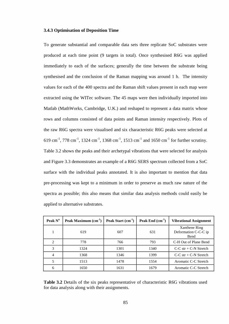
Table 3.2 Details of the six peaks representative of characteristic R6G vibrations used
for data analysis along with their assignments. ............................................................... 85
Table 3.3 Global averages for R6G peak intensities from Raman maps (20*20 pixels)
including all 400 spectra with corresponding %RSDs for each peak at the three
deposition times investigated. ......................................................................................... 90
Table 3.4 Correlation coefficients for the mean and %RSD for each peak in the R6G
spectra with respect to temperature.. ............................................................................... 90
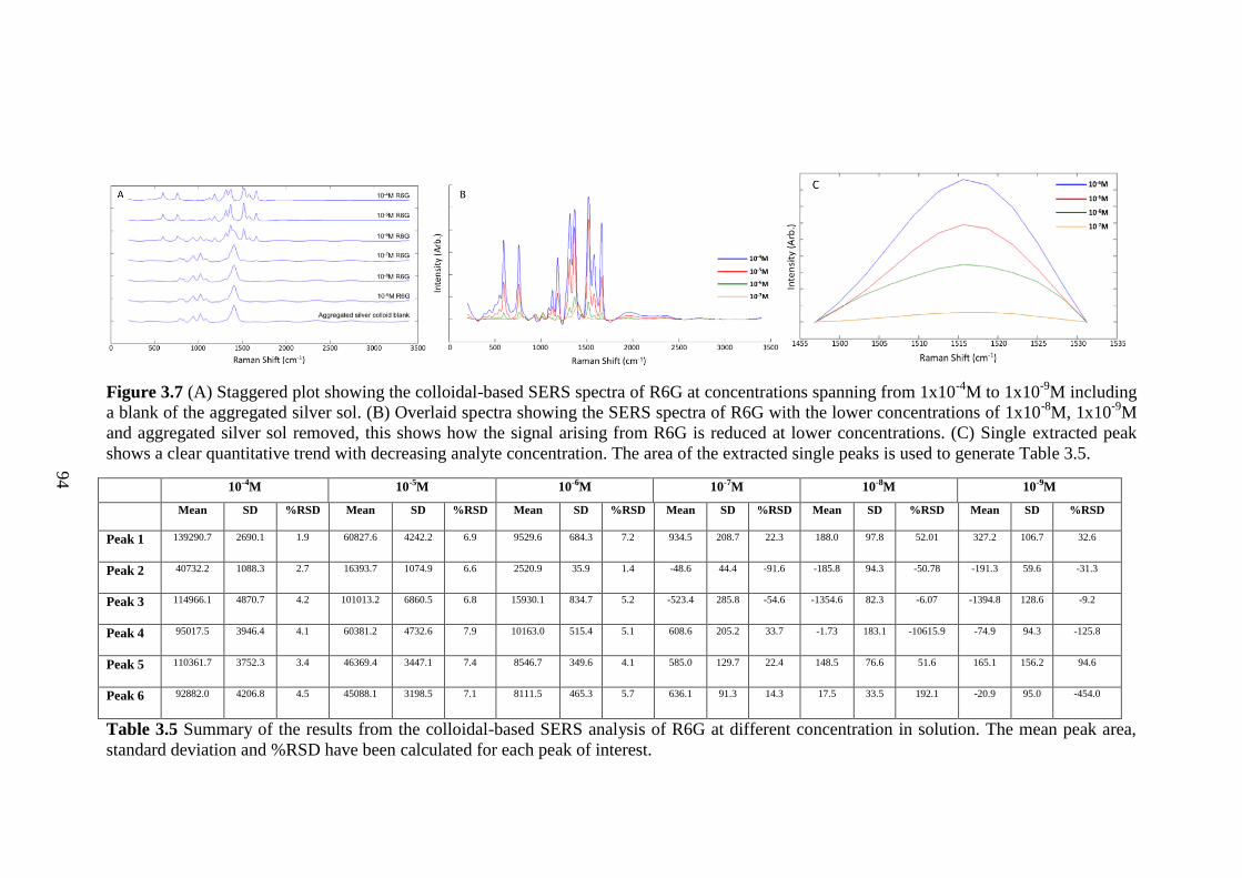
Table 3.5 Summary of the results from the colloidal-based SERS analysis of R6G at
different concentrations in solution. ................................................................................ 94
Table 4.1 The seven common R6G peaks used for analysis are shown together with
vibrational assignments ................................................................................................. 112
Tables 4.2a-e Mean peak areas (trapezoidal and sum integration), mean intensities and
mean RSDs calculated for Klarite 1-5 .......................................................................... 113
Tables 4.3a-e Mean peak areas (trapezoidal and sum integration), mean intensities and
mean RSDs calculated for QSERS 1-5 ......................................................................... 116
Tables 4.4a-e Mean peak areas (trapezoidal and sum integration), mean intensities and
mean RSDs calculated for SoC 1-5 ............................................................................... 119
Table 4.5 Mean RSDs calculated across all peak areas an intensities for assessment of
batch to batch reproducibility (repeatability) ................................................................ 122
Table 4.6 The calculated mean number of noisy spectra and estimated percentage R6G
coverage across all substrate replicates ......................................................................... 123
Page 6
6
Table 4.7 A traffic light based summary of the substrates performance. ..................... 127
Table 4.8 The relationship between the variation in RSD and the number of spectra
collected. ....................................................................................................................... 128
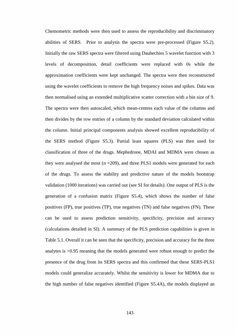
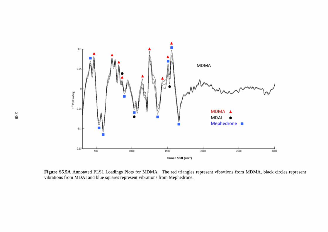
Table 5.1 Summary of the results generated from PLS for each of the drugs analysed
....................................................................................................................................... 144
Table 6.1 UV-vis spectrophotometry results of the silver sol batches with calculated λ
max and full width half maximums (FWHM). ............................................................. 154
Table 6.2 Optimised aggregation times MDAI detailed for the different colloidal
batches and respective salt concentrations. ................................................................... 159
Table 6.3 MDAI reproducibility results. ...................................................................... 161
Table 6.4 Tentative SERS vibrational assignments for the 7 peaks identified for MDAI.
....................................................................................................................................... 163
Table 7.1 Tentative SERS vibrational assignments for Mephedrone .......................... 176
Table 7.2 A summary of the results for the reproducibility analysis for the two pH
optimums ....................................................................................................................... 182
Table 7.3 A summary of the results for the reproducibility analysis for the two salt
optimums ....................................................................................................................... 183
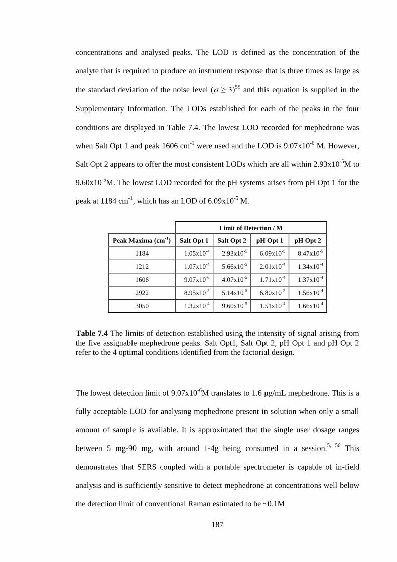
Table 7.4 The limit of detection established using the intensity of signal arising from
the five assignable mephedrone peaks. ......................................................................... 187
Table 8.1 Tentative SERS vibrational assignments for ampicillin. ............................. 204
Table 8.2 Tentative SERS vibrational assignments for carbenicillin. .......................... 204
Table 8.3 Tentative SERS vibrational assignments for ticarcillin. .............................. 205
Table 8.4 Vibrational assignments for the hydrolysis of ampicillin. ........................... 210
Table 8.5 Correlation analysis results for each peak area analyses for ampicillin. ...... 212
Page 7
7
List of Figures
Figure 1.1 Electromagnetic wave propogation. ............................................................. 18
Figure 1.2 The Jablonski diagram showing the electronic and vibrational states of a
molecule. ......................................................................................................................... 21
Figure 1.3 Diagrammatic representation of fluorescence emission. .............................. 23
Figure 1.4 Diagrammatic representation of Rayleigh and Raman scattering. ............... 25
Figure 1.5 Diagrammatic representation of the Morse potential ................................... 28
Figure 1.6 The three modes of vibration for a water molecule ...................................... 32
Figure 1.7 A Raman microscope system and its internal and external components. ..... 35
Figure 1.8 A diagrammatic representation of CARS. .................................................... 37
Figure 1.9 A diagrammatic representation of HRS. ....................................................... 38
Figure 1.10 Metal nanoparticles and their plasmonic waves. ........................................ 42
Figure 2.1 Optical images of gold and silver sols .......................................................... 59
Figure 2.2 TEM micrographs of the gold and silver nanoparticles synthesised using
citrate reduction. .............................................................................................................. 60
Figure 2.3 Optical images of glass slides functionalized with gold and silver
nanoparticles. .................................................................................................................. 61
Figure 2.4 SEM images of gold and silver nanoparticles bound to a silicon support .... 63
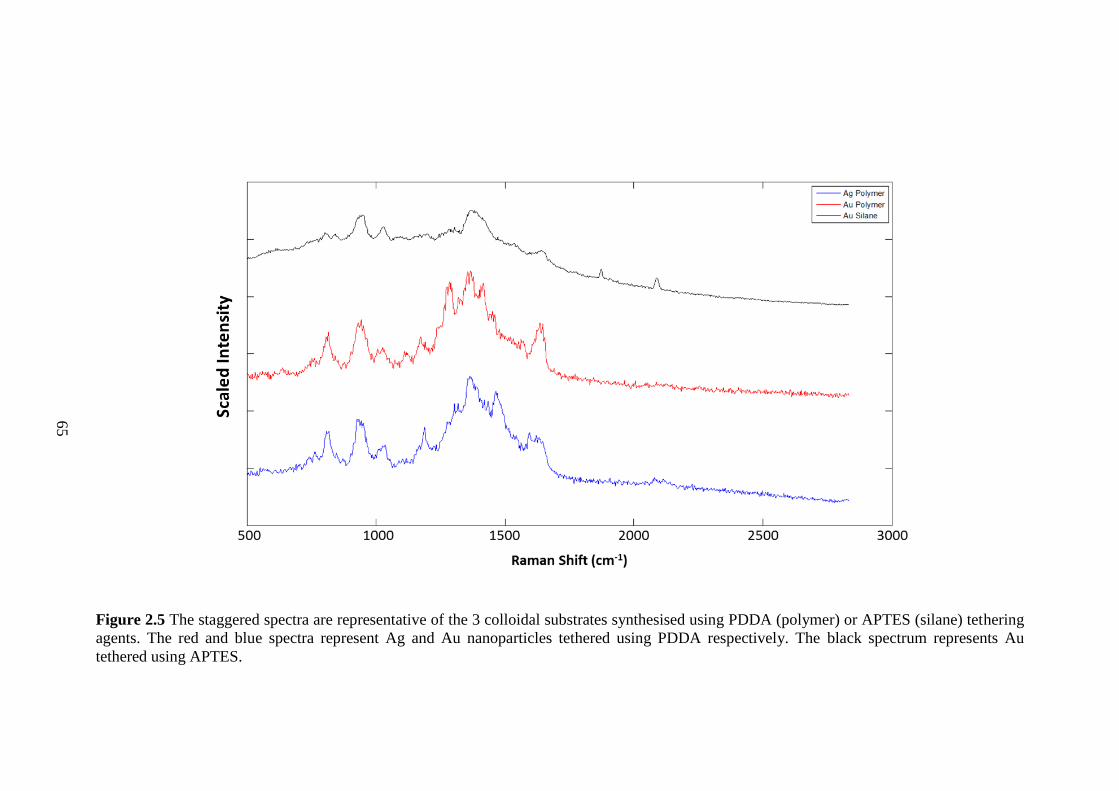
Figure 2.5 Spectra representative of the three colloidal substrates synthesised using
PDDA (polymer) or APTES (silane) tethering agents. ................................................... 65
Figure 2.6 SEM image of a single silver nanocluster. ................................................... 67
Figure 2.7 SEM image of the nanoplate formation in acid erosion sites. ...................... 68
Figure 2.8 SEM image of silver nanocluster deposits on aluminium foil ...................... 69
Page 8
8
Figure 3.1 SEM images taken of the silver on copper (SoC) substrate at a range of
deposition times and temperatures.. ................................................................................ 81
Figure 3.2 Optical image showing the border of the silver deposition site,
corresponding SERS chemical map, SERS spectrum of R6G and Raman spectrum of
blank copper .................................................................................................................... 84
Figure 3.3 A typical SERS spectrum of 10-4
M R6G acquired on the SoC surface ........ 86
Figure 3.4 The global averages calculated for the peaks 1-6 (A-F) at each optimisation
temperature (23-100oC). .................................................................................................. 89
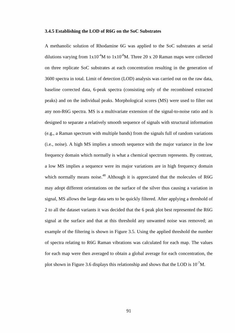
Figure 3.5 Illustration of morphological scores filtering for removal of non-R6G SERS
spectra from the data set. ................................................................................................. 92
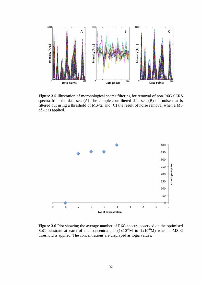
Figure 3.6 Plot showing the average number of R6G spectra observed on the optimised
SoC substrate at each of the concentrations (1x10⁻⁴
M to 1x10⁻⁸
M) when a MS>2
threshold is applied ......................................................................................................... 92
Figure 3.7 Staggered plot showing the colloidal-based SERS spectra of R6G at
concentrations spanning from 1x10⁻⁴
M to 1x10⁻⁹
M........................................................ 94
Figure 3.8 The PCA scores plot showing the R6G concentration clustering. ................ 95
Figure 3.9 Loadings plot representative of separation across PC1 for the differing
concentrations of R6G..................................................................................................... 96
Figure 4.1 SEM images of the three SERS substrates (SoC, Klarite and QSERS). .... 107
Figure 4.2 Mean SERS spectra (n=6400) generated on each of the Klarite substrate
replicates.. ..................................................................................................................... 108
Figure 4.3 Mean SERS spectra (n=6400) generated on each of the QSERS substrate
replicates.. ..................................................................................................................... 109
Figure 4.4 Mean SERS spectra (n=6400) generated on each of the SoC substrate
replicates.. ..................................................................................................................... 109
Page 9
9
Figure 4.5 Example SERS maps generated based on the total peak area of the 7
processed and recombined R6G peaks. ......................................................................... 123
Figure 4.6 SERS chemical maps and plots representative of signal and noise
discrimination of R6G on Klarite 4.. ............................................................................. 124
Figure 4.7 SERS chemical maps and plots representative of signal and noise
discrimination of R6G on QSERS 4.. ........................................................................... 124
Figure 4.8 SERS chemical maps and plots representative of signal and noise
discrimination of R6G on SoC 5. .................................................................................. 125
Figure 4.9 PCA plot calculated for SoC 5. ................................................................... 125
Figure 5.1 SEM Characterisation of galvanic displacement of silver onto a British 2p
coin ................................................................................................................................ 140
Figure 5.2 Chemical maps of R6G deposited on the coins surface.............................. 142
Figure 5.3 Average SERS spectra from Mephedrone (n=56), MDAI (n=109) and
MDMA (n=36). ............................................................................................................. 142
Figure 6.1 Molecular structure of MDAI with numbers for NMR assignment. .......... 148
Figure 6.2 UV-vis spectrophotometry results for the five silver colloidal batches...... 153
Figure 6.3 Average spectra of each batch of colloid generated through the optimisation
of aggregation experiment............................................................................................. 158
Figure 6.4 An example plot for demonstrating the determination of optimum
aggregation time.. .......................................................................................................... 159
Figure 6.5 Overlayed SERS spectra for the optimised blank and MDAI. ................... 162
Figure 6.6 Plots of peak area versus concentration for the seven identified MDAI peaks.
....................................................................................................................................... 163
Figure 7.1 PCA scores plots computed on the SERS intensities of the 10 mephedrone
peaks under study.. ........................................................................................................ 179
Page 10
10
Figure 7.2 Example raw SERS spectra of mephedrone (5x10⁻⁴
M) acquired using all the
conditions identified by the factorial design.. ............................................................... 184
Figure 8.1 Molecular structures of ampicillin, carbenicillin and ticarcillin. ................ 196
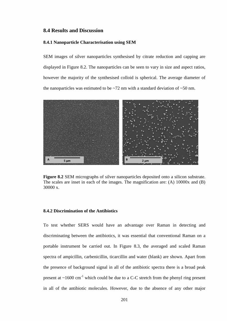
Figure 8.2 SEM images of silver nanoparticles. .......................................................... 201
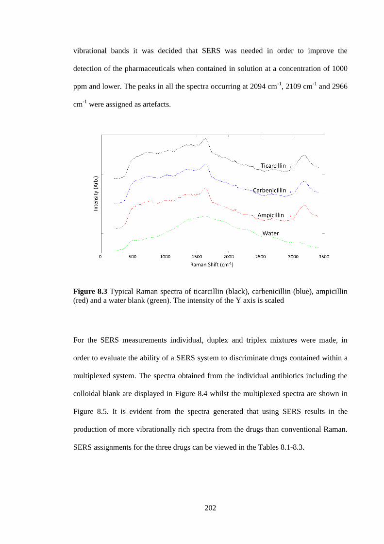
Figure 8.3 Typical Raman spectra of the individual antibiotics including a water blank.
....................................................................................................................................... 202
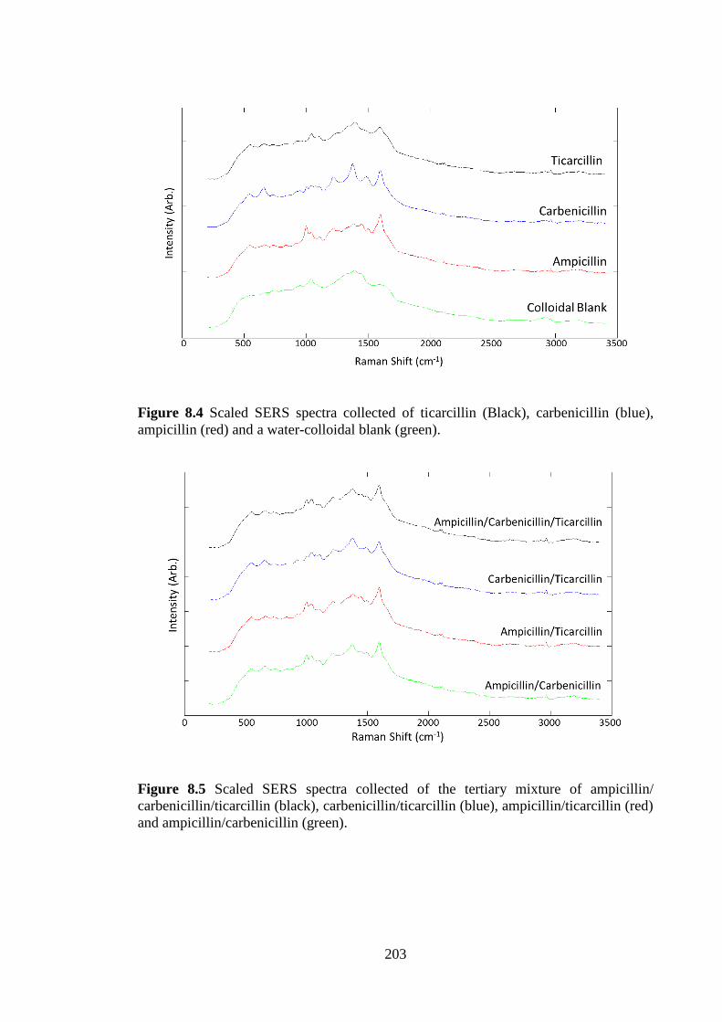
Figure 8.4 SERS spectra of the individual antibiotics including a water blank. .......... 203
Figure 8.5 SERS spectra of the binary and tertiary antibiotic mixtures ....................... 203
Figure 8.6 PCA plot of the individual, duplexed and triplexed antibiotic SERS samples.
....................................................................................................................................... 206
Figure 8.7 Derivation of the optimum concentration and aggregation time for following
the hydrolysis of ampicillin. .......................................................................................... 208
Figure 8.8 SERS Spectra of 10 ppm ampicillin under varying pH conditions.. .......... 209
Figure 8.9 Plots of peak area with respect to pH for changing ampicillin vibrations. . 211
Figure 8.10 ESI-Mass spectra of ampicillin at pH 7.16. .............................................. 213
Figure 8.11 ESI-Mass spectra of ampicillin at pH 1.96 ............................................... 214
Page 11
11
List of Schemes
Scheme 2.1 The process for the production of SERS substrates through the adherence
of nanoparticles to a glass slide ....................................................................................... 58
Scheme 3.1 Redox reaction showing the galvanic displacement of silver onto copper. 75
Scheme 8.1 Proposed mechanism for the acid hydrolysis of a β-lactam ring.. ............ 196
Page 12
12
Abstract
The University of Manchester
Samuel Bernard Mabbott
Doctor of Philosophy
Optimisation of Solid-State and Solution-Based SERS Systems for use in the Detection
of Analytes of Chemical and Biological Significance
13th
September 2012
Surface enhanced Raman scattering (SERS) has achieved much attention since its
conception in 1974. The analytical technique overcomes many difficulties associated
with conventional Raman whilst also increasing sensitivity. However, the increased
interest and work in the field has also identified flaws, many of which are centred on the
irreproducibility of the SERS enhancement effect. The majority of the work described
in this thesis focusses on the ‘optimisation’ of solid-state and solution based SERS
systems. Optimisation plays a crucial role in maximising both enhancement effects and
reproducibility. Here criteria are outlined for the synthesis of high performance solid-
state SERS substrates and the synthesis of a range of substrates is assessed, each with
associated pros and cons. The most successful substrate was synthesised by exploiting
redox potentials which allow for the direct deposition of silver onto copper foil. The
deposition times and temperatures were optimised sequentially to generate a high
performance substrate capable of detecting Rhodamine 6G at trace levels.
Reproducibility comparisons of the silver on copper (SoC) substrate were carried out
against commercial substrates: Klarite and QSERS, multiple univariate and multivariate
methods were used to assess the substrates performance. The results confirmed that the
SoC substrate performed better than both the commercial substrates. The work also
highlights the importance of using multiple data analysis methods in order to assess the
performance of a solid-state SERS substrate. Deposition of the silver surface was also
successful on British 2p coins allowing the for the detection and discrimination of
illegal and legal drugs when coupled with multivariate data analysis methods such as
PCA and PLS. Solution based SERS analyses were also carried out successfully using
different optimisation strategies. The initial investigation involved careful control of the
individual components of a SERS system (nanoparticles, aggregating agents and
analyte) in order to establish a low limit of detection for the increasingly abused ‘legal
high’ MDAI. The use of a reduced factorial design was then successfully employed to
explore a greater number of SERS variables and define a low limit of detection for the
class B drug mephedrone. The robust experimental design also allowed an insight into
the importance of each of the individual components within a solution based SERS
system. The final piece of work carried out was the SERS discrimination of antibiotics:
ampicillin, ticarcillin and carbenicillin. Optimisation of the solution based experiment
allowed the in-situ hydrolysis of the β-lactam moiety present in ampicillin rendering it
pharmacologically inactive to be followed under acidic conditions at concentrations of
10 ppm.
Page 13
13
Declaration
No portion of the work referred to in this thesis has been submitted in support of an
application for another degree or qualification of this or any other university or other
institute of learning
Page 14
14
Copyright Statement
i. The author of this thesis (including any appendices and/or schedules to this
thesis) owns certain copyright or related rights in it (the “Copyright”) and s/he
has given The University of Manchester certain rights to use such Copyright,
including for administrative purposes.
ii. Copies of this thesis, either in full or in extracts and whether in hard or
electronic copy, may be made only in accordance with the Copyright, Designs
and Patents Act 1988 (as amended) and regulations issued under it or, where
appropriate, in accordance with licensing agreements which the University has
from time to time. This page must form part of any such copies made.
iii. The ownership of certain Copyright, patents, designs, trademarks and other
intellectual property (the “intellectual Property”) and any reproductions of
copyright works in the thesis, for example graphs and tables (“Reproductions”),
which may be described in this thesis, may not be owned by the author and may
be owned by third parties. Such Intellectual Property and the Reproductions
cannot and must not be made available for use without the prior written
permission of the owner(s) of the relevant Intellectual Property and/or
Reproductions.
iv. Further information on the conditions under which disclosure, publication and
commercialisation of this thesis, the Copyright and any intellectual Property
and/or Reproductions described in it may take place is available in the
University IP Policy (see
http://www.campus.manchester.ac.uk/medialibrary/policies/intellectual-
property.pdf), in any relevant Thesis restriction declarations deposited in the
University Library, The University Library’s regulations (see
http://www.manchester.ac.uk/library/aboutus/regualtions) and in The
University’s policy on presentation of Theses.
Page 15
15
Abbreviations
AFM Atomic Force Microscopy
APTES (3-aminopropyl)triethoxysilane
CARS Coherent Anti-Stokes Raman Spectroscopy
CCD Charge Coupled Device
EDX Energy Dispersive X-ray Analysis
EF Edge Filter
ESI(MS) Electrospray Ionisation Mass Spectrometry
FFD Fractional Factorial Design
GD Galvanic Displacement
GMT Generalised Mie Theory
HOMO Highest Occupied Molecular Orbital
HNF Holographic Notch Filter
HPLC High Performance Liquid Chromatography
HRS Hyper Raman Spectroscopy
IR Infrared Spectroscopy
KHD Kramer Heisenberg Dirac equation
Laser Laser Amplification by Stimulated Emission of Radiation
LUMO Lowest Unoccupied Molecular Orbital
MDAI 5,6-methylenedioxy-2-amino indane
MDMA 3,4-methylenedioxy-N-methyl amphetamine
MFON Metal films over nanospheres
MPTES (3-mercaptopropyl)triethoxysilane
MS Morphological scores
Nd:YAG Neodymium-doped Yttrium Aluminum Garnet
NMR Nuclear Magnetic Resonance spectroscopy
PCA Principal Components Analysis
PLS Partial Least Squares
R6G Rhodamine 6G
RSD Relative Standard Deviation
SD Standard Deviation
SEM Scanning Electron Microscopy
SERS Surface enhanced Raman scattering
SMSERS Single molecule surface enhanced Raman scattering
SNOM Scanning near-field optical microscopy
SoC Silver on Copper substrate
SOE Sparcity Of Effects
STEM Scanning Tunneling Microscopy
TEM Transmission Electron Microscopy
TERS Tip-enhanced Raman Scattering
UV Ultraviolet
UV-vis UV-visible Spectrophotometry
Page 16
16
Acknowledgements
Firstly, I would like to thank my supervisor, Professor Royston Goodacre, without him
the chance to explore such an engaging subject would have been impossible. His belief
and constant reassurance when in times of doubt has provided me with constant
motivation throughout my studies.
Secondly, I would like to thank Will Allwood, David Cowcher, Victoria Brewster and
Yu Xu, who have provided me endless amounts of support during my time in
Manchester. Thanks to all the members of the research group; past and present, little
bits of advice here and there have often made the difference between success and
failure. I would also like to extend this thanks to all the third year and fourth year
project students whom I have had the pleasure of mentoring.
Completing this work would be more difficult were it not for the Strathclyde group
under the supervision of Duncan Graham and Karen Faulds who granted me open
access to their instrumentation and have since allowed my journey through academia to
continue. I would especially like to express my gratitude to Iain Larmour who helped
nurture my knowledge in the field from the very beginning. Thanks also go to Cinzia
Casiraghi and Axel Eckman who also granted me immediate access to their Raman
instrument when time was of the essence.
I must express my gratitude to my girlfriend Hannah, who has had to put up with my
lows and heard endlessly about my highs. For the tolerance, encouragement and support
I am hugely grateful.
Last but not least, I would like to thank my Brother, Ben who has always helped me to
put things in perspective and has made me laugh even when I have been struggling to
see the funny side. This thesis is however dedicated to my Mum and Dad who have
nurtured me through this whole process, their unconditional love and support has seen
me through some difficult times, for that I am most appreciative. I hope this makes you
proud.
“Anyone who has never made a mistake has never tried anything new.”
Albert Einstein
Page 17
17
1. Introduction
Page 18
18
1.1 The Electromagnetic Spectrum and its Wave/Particle Duality
Relationship
Light is a form of electromagnetic radiation that can be characterised according to the
electromagnetic spectrum. It is essential that the properties of light are discussed as it
plays a central role in the spectroscopic interrogation of samples.
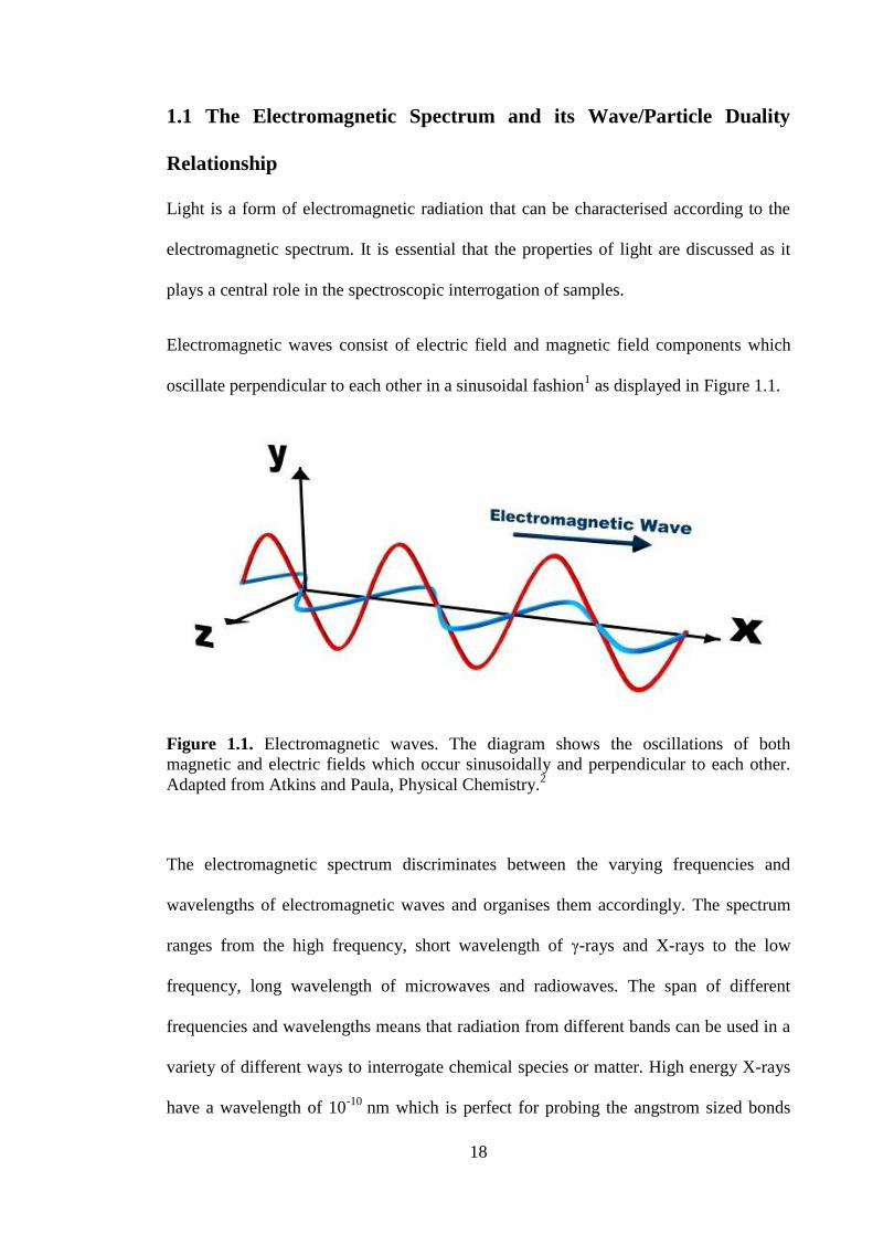
Electromagnetic waves consist of electric field and magnetic field components which
oscillate perpendicular to each other in a sinusoidal fashion1 as displayed in Figure 1.1.
Figure 1.1. Electromagnetic waves. The diagram shows the oscillations of both
magnetic and electric fields which occur sinusoidally and perpendicular to each other.
Adapted from Atkins and Paula, Physical Chemistry.2
The electromagnetic spectrum discriminates between the varying frequencies and
wavelengths of electromagnetic waves and organises them accordingly. The spectrum
ranges from the high frequency, short wavelength of γ-rays and X-rays to the low
frequency, long wavelength of microwaves and radiowaves. The span of different
frequencies and wavelengths means that radiation from different bands can be used in a
variety of different ways to interrogate chemical species or matter. High energy X-rays
have a wavelength of 10-10
nm which is perfect for probing the angstrom sized bonds
Page 19
19
contained within crystalline structures, whereas the long radiowaves have particular use
in probing a molecules environmental spin properties and are essential to the operation
of NMR. The relationship between a waves frequency and wavelength is defined by
Equation 1.1, where = frequency (Hz), = wavelength (nm) and = speed of light
(299792458 ms-1
)
(1.1)
The most important area of the electromagnetic spectrum in relation to this thesis is the
region populated by infra-red, visible and ultra-violet radiation. It is this portion of the
spectrum that allows details on a species molecular vibrations and rotations to be
observed, hence the radiation here has been harnessed for optical vibrational
spectroscopy.3,4,5
Maxwell Planck was the first among many scientists who successfully hypothesised the
wave/particle duality of electromagnetic radiation. He demonstrated using the black
body radiation experiment6 that electromagnetic radiation or light waves can be broken
down into discrete packets of energy (quantizations) all relating to the frequency of
oscillations. Viewing light as a single entity with zero mass oscillating in a wave at the
speed of light is derived from quantum theory.7,8
Planck’s physical constant, (6.626 x
10-34
J.s) is a proportionality constant that provides the relationship between frequency
and the energy of the photon, shown in Equation 1.2.
(1.2)
Energy can also be easily related to the component values of light waves: speed of light
in a vacuum (C), wavelength (λ) and frequency ( through Equation 1.3
Page 20
20
(1.3)
In some circumstances when the frequency of the light waves is expressed in radians per
second instead of cycles per second ( it is necessary to use the reduced Plancks
constant ( ) and an alternative energy equation shown in Equation 1.4
(1.4)
When trying to interpret the interaction light has with matter, it is much simpler to view
light interacting as a particle (photon) rather than a wave. Light can also be categorised
according to the interactions it has with samples, these categories are absorption,
scattering and emission, with scattering being the most relevant event to this thesis. The
probability of any of the events occurring is entirely dependent on the molecule being
analysed and its component energy states. To interpret these differing states a Jablonski
diagram is used (Figure 1.2), this describes the molecules in terms of quantum states
and builds a hierarchy of discrete energy levels by which each molecular vibration and
interaction can reside depending on excitation. The Jablonski diagram can be split into
two main transitions, electronic and vibrational. The tighter lines represent vibrational
energy transitions, so the energy needed for these transitions to occur is reduced in
comparison to the wider energy level gaps, found between the ground and excited states
representing electronic transitions.
Page 21
21
Figure 1.2 The Jablonski diagram shows the electronic and vibrational energy states of
a molecule and illustrates the transitions between them. The states are arranged
vertically by energy. The two types of electronic relaxation modes displayed on the
diagram are fluorescence and phosphorence.
It is now necessary to address each individual interaction separately. Absorption and
emission will be discussed briefly in this section to further develop the understanding
behind the interactions, whilst the section on Raman scattering will discuss scattering
effects in more detail.
Page 22
22
1.2 Radiation and Analyte Interactions
1.2.1 Absorption
There are two different ways in which absorption can be interpreted; one interpretation
concerns the process associated with vibrational transitions whilst the other involves
electronic transitions. The absorption process which results in the promotion of a
molecule from a lower vibrational energy level to a higher vibrational state within the
electronic ground state is associated with the fundamental operation of IR spectroscopy.
Whilst the alternative type of absorption involves the absorbance of energy causing a
transition from the electronic ground state to an electronic excited state. Absorption
occurs when the energy of the incoming light wave or photon is near identical to the
energy levels of the electrons contained within the matter. It is vital that the frequency
of the electromagnetic radiation matches the frequency of the molecule for absorption to
occur.
1.2.2 Emission
The spontaneous emission of energy from a molecule can occur by two processes;
fluorescence and phosphorescence. The emission that is most prevalent, yet problematic
to Raman spectroscopy is fluorescence. Fluorescence is caused when a molecule
absorbs a photon, lifting it into an excited state, once in this excited state energy gets
emitted which is equal to the energy of each of the lower vibrational levels. The energy
emitted at each state, is much lower than the photon that was initially absorbed.8 A large
majority of the energy will be transferred as molecular vibrations and rotations,
however the problem for Raman comes when the energy is emitted as a photon with a
wavelength and frequency that corresponds to the visible region of the electromagnetic
spectrum Figure 1.3 shows the fluorescence cycle. Within this visible region is where
Page 23
23
the Stokes lines reside, so interference from fluorescence can cause masking of the
spectral fingerprint. This problem is much bigger when using a powerful, visible
radiation source.9 In-order to overcome the fluorescence problem, it is first necessary to
try a number of different laser lines of varying frequencies.10,11
Figure 1.3 Fluorescence occurs when an electron contained within a molecule relaxes
from an electronic excited state down to the ground state. The emission of red shifted
photons of a lower energy is characteristic of fluorescence and can be detrimental to
Stokes Raman signal.
Typical relaxation times of fluorescence differ from 0.5 to 20 ns depending on the type
of emission. There are a few ways in which fluorescence can be suppressed in Raman
analyses. These include the use of a Kerr-gate system,12
photo-bleaching,13
SERS and if
Page 24
24
the fluorescence is still a problem the system can be arranged so it could detect the anti-
Stokes spectrum of the species.14
Phosphorescence is an effect whereby photons are ejected by the molecule over a much
longer time span.15
On a basic level the molecule can be seen to store energy, but it is
necessary to revert to quantum explanations to understand this type of emission fully.
The molecule absorbs energy from the photon and gets promoted to the singlet excited
levels, in the same way as fluorescence. However phosphorescent materials contain
triplet states to which the molecule crosses into via a phenomena called inter-system
crossing (Figure 1.2) once contained within these triplet states, quantum rules dominate.
Classically forbidden transitions are necessary to return the excited molecule back down
to its ground state. Although these transitions occur, kinetically they are highly
unfavourable and relaxation is extremely slow, this is why emission of photons from a
phosphorescent material is a prolonged event. Emission lifetime is dependent on the
quantum yield of the material, but times can range from nanoseconds to hours.
Phosphorescence is a property of a unique class of chemicals,16
and never has to be
compensated for in Raman spectroscopy.
Page 25
25
1.3 Theory of the Raman Effect
1.3.1 The Raman Effect
Light interaction with a molecule or atom can produce two types of fundamental
scattering relevant to this work, these are: Rayleigh and Raman. The photon evolved in
Rayleigh scattering retains the same frequency of the light source from which it is
produced, Raman scattering however involves an exchange of energy between the
photon and the analyte resulting in an energetic gain or loss during the process.3,17
The
two forms of scattering are known as elastic and inelastic respectively. It is however the
latter process with which we are concerned, because of the detailed amount of chemical
information the energy change gives us about the unique vibrational modes within a
molecule. The Raman scattering process can be further broken down into two types of
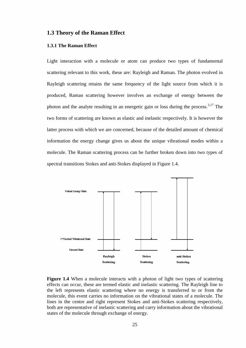
spectral transitions Stokes and anti-Stokes displayed in Figure 1.4.
Figure 1.4 When a molecule interacts with a photon of light two types of scattering
effects can occur, these are termed elastic and inelastic scattering. The Rayleigh line to
the left represents elastic scattering where no energy is transferred to or from the
molecule, this event carries no information on the vibrational states of a molecule. The
lines in the centre and right represent Stokes and anti-Stokes scattering respectively,
both are representative of inelastic scattering and carry information about the vibrational
states of the molecule through exchange of energy.
Page 26
26
The Stokes transition occurs when a photon interacts with a molecule whose energy is
observed within the ground state. The interaction results in the photons transferral of
energy to the molecule thus promoting it to a higher vibrational energy level. The anti-
Stokes transition has the opposite effect.18
The molecule already resides in an excited
ground state vibrational level and interaction with an incident photon involves exchange
of energy from the molecule to the photon, quenching the excited molecule back down
to its ground state. The intensity of the Stokes or anti-Stokes spectra is therefore
dependent upon the thermal distribution of molecules, if a thermal equilibrium is
reached the relative numbers of molecules in different energy states can be given by the
Boltzmann equation2 displayed in Equation 1.5, where : number of particles in the
excited vibrational state, : number of particles in the ground vibrational state, :
degeneracy in the excited state, : degeneracy in the ground state, ( :
difference in energy beween the two states, : Boltzmann constant (1.3806503 × 10⁻²³
m2 kg s
-2 K
-1), : Temperature (K). As a greater population of molecules exist in the
ground state the Stokes lines are much more intense than the anti-Stokes.
(
) ( ( ) (1.5)
Both of these energy transitions adhere to the conservation of momentum; at no point is
energy removed from the system. It must be also outlined that the mechanism for
energy exchange in relation to Raman scattering is concerted, meaning this is an
instantaneous process in which energy transferral between the molecule and
incident/resultant photons cannot be split into two parts and are independent of time.
Raman scattering is the much weaker analogue of the two scattering effects with only ~
1 in 106 - 10
8 photons being scattered in this way, but both Rayleigh and Raman
scattering both adhere to an identical power law.9,15
The law relates the efficiency of
Page 27
27
scattering to the third power optical frequency. This means that light of much smaller
wavelengths give an enhanced scattering effect. Although it may be simple to theorise
that a smaller more energetic wavelength will give intense scattering, experimentally
this approach may not be ideal as wavelengths with more energy can lead to the
electronic transitions of a molecule causing fluorescence.8
As mentioned before the energy loss or gain during an interaction relates to the energies
of the rotational and vibrational modes of a molecule. The energy exchange signifies the
net energies of all the modes present, by dissecting this energy into the individual
quantum levels or states we can relate back to the structural composition of a molecule.
1.3.2 Morse Curve
The use of Hooke’s law, combined with the Morse curve means that Raman spectral
bands can be interpreted according to the vibrational mode they represent. Figure 1.5
displays the Morse curve. Here the red line represents the energy observed between a
pair of atoms. Initially the energy is high as the atoms are essentially free, but as the
atoms start to become attracted, distance decreases along with energy. After observation
of the minimum the atoms get too close and start to repel each other raising the energy.
The minimum is representative of the bond formation energy and also indicates the
bond length.
Page 28
28
Figure 1.5 The Morse potential (red line) describes the energy of a bond, dependent on
nuclear distance. The blue solid lines are representative of the harmonic oscillator
potential which describe the vibration states of an atom
Ideally the curve would represent all the energies that could be achieved, but because
the vibrational energies are quantized they have to be broken into separate quantized
vibrational levels represented in Figure 1.5 by the blue lines labelled ν = 0, 1, 2 etc...
The Morse curve displayed is representative of only one molecular vibration and is very
simplistic in describing what actually happens in Raman scattering, however does
provide a good approximation. The band ν = 0 represents the ground state of the
molecule here there has been no uptake of energy to allow for molecular vibrations. In
order to progress to the second level (ν = 1) the molecule has to absorb one quanta of a
precise energy corresponding to the band gap; this transition is called the fundamental.
Progression to higher energy levels requires absorption of specific numbers of quanta.
The curve however does not give an indication of the lower energy rotational levels and
Page 29
29
for it to be completely applicable to Raman scattering more Morse curves would have to
be drawn for each vibronic state because even these have an influence on scattering
efficiency.2,9
Using the Morse curve to estimate the energy of the vibronic levels is very
difficult, so it is necessary to introduce a harmonic approximation. This approach
replaces the curve with a parabola calculated for a diatomic molecule, and uses Hooke’s
law to define the relationships between frequency, mass of atoms and bond strength.
1.3.3 Hooke’s Law
To understand Hooke’s law, the vibrational bond has to be visualised as two masses
(atoms) connected by a spring (the bond). The equations in 1.6 allows the approximate
frequency of vibrations to be calculated according to which atoms are involved in the
bond
√
(1.6)
Here represents the reduced mass of atoms a and b with masses of and
respectively, is the force constant and is the speed of light.
By following this law it can be approximated that, the lighter the atoms, vibrate at
higher frequencies. It can be seen that species such as amines have high frequencies
spanning the range 3200-3500 cm-1
,19
representative of the light atoms which comprise
the bond. On the other extreme are carbon-halogen bonds whose frequencies are
inherently low due to the presence of a heavy halogenic atom.19
The monochromatic light used as an excitation source in Raman scattering can be at
least partially polarized.9 Many Raman spectrometers will contain a polarizer which
Page 30
30
essentially specifies the electromagnetic waves direction causing the light to become
linearly polarized. Light of this character can distort the electron cloud surrounding the
molecule, and the extent to which the electron cloud becomes distorted depends on the
on the electrons ability to polarize. Polarizability is the effect that gives rise to Raman
scattering events.
1.3.4 Polarizability
Although the light falling upon a molecule in linearly polarized the electron cloud
becomes perturbed in all directions, giving rise to dipole changes on all three Cartesian
co-ordinates x, y and z. There are two ways of expressing the dipole change in a
molecule these are the simple evaluation in Equation 1.7 and a tensor shown in
Equation 1.8.
(1.7)
Where is the induced dipole, is polarization and is the electric field charge.
[
] [
] [
] (1.8)
The subscripts eg in the matrix represent the direction of polarizability of the
molecule and the polarization of the incident light respectively. The normal modes or
vibration of molecules are Raman active if they are accompanied by a changing
polarizability.20
To understand Raman active vibrational modes fully it would be
necessary to study the symmetry elements and then identify the point group of the
analyte of interest, but because the chemicals and specimens of interest to this thesis
contain complex structures this type of analytical depth is not essential. A brief example
will be given for water, describing why it is a weak Raman scatterer.
Page 31
31
1.3.5 Raman Active Vibrations of Water and Mutual Exclusion
As already mentioned, for a vibrational mode to be Raman active it must involve a
change in polarizability of the molecule4 ( ) Equation 1.9 shows how a change in
polarization effects the equilibrium position (e) from the normal coordinate (q)
(
)
(1.9)
Raman spectroscopy is complementary to Infrared (IR) spectroscopy in that for a
centrosymmetric molecule, Raman active modes are IR inactive and vice versa. This
rule is termed mutual exclusion, however this rule does not apply to water as the point
group C2v to which water belongs contains no centre of symmetry. Water has a bent
structure consisting of an oxygen atom bound to two hydrogen atoms, the number of
vibrational modes of water can be estimated using the vibrational degrees of freedom
(Equation 1.10). As translational energy can be described in terms of three vectors 90o
to each other it is said that there is three degrees of freedom, rotational energy can also
be described as having three degrees of freedom. For linear molecules however this
freedom is limited to a value of two degrees as the molecule is only able to rotate
around or about the axis. The equations therefore used to estimate the number of
vibrations is displayed in 1.10 for non-linear molecules and 1.11 for linear molecules,
where N is the number of atoms.
(1.10)
(1.11)
The number of observable vibrations for water is therefore three. Figure 1.6 shows
which vibrations are responsible for the modes.19
Page 32
32
Figure 1.6 The three modes of vibration for a water molecule are displayed. All
vibrational modes are Raman active but the bending mode and asymmetric stretch only
display a small change in polarizability so are very weak and so do not feature on a
Raman spectrum. The polarizability change in the symmetric stretch is much greater so
can be seen in Raman spectra.
All three of water’s vibrational modes are Raman active as each involves a change in
polarizability, however the magnitude of change is different for each mode. The
bending mode and asymmetric stretch for water show only small amounts of
polarizability change so they are very weakly Raman active, and will have no visible
peaks present on a Raman spectrum. By contrast the symmetric stretch however
undergoes a greater change in polarization and therefore can be seen on a Raman
spectrum. Although all the modes are Raman active they are not as intense as the bands
seen in an IR spectrum this is because all the modes display a change of dipole as the
atoms vibrate through their equilibrium positions. Due to water being such a weak
Raman scatterer, analysis of biological systems which reside in an aqueous environment
is much easier with little or no interference coming from the water itself. The intensity
of Raman scattering is defined using Equation 1.12 where, K is representative of the
speed of light, l is the laser power, the frequency of the incident radiation and α is the
polarizability of electrons in the molecule.9
Page 33
33
(1.12)
Now the main underlying theories of the Raman effect has been addressed the
instrumental components of a Raman system can be discussed.
1.4 Raman Instrumentation
1.4.1 Components of a Raman System
Each component of the spectrometer plays a vital role in the retrieval and interpretation
of the Raman signal. Figure 1.7 displays the integral components which make up a
Raman microscope system. The laser light source provides monochromatic sample
illumination. The photons produced by the laser interact with the analyte molecules
causing perturbation of its vibrational modes.
There are a range of lasers available for Raman instruments with the most common
lasers used residing in the visible region of the electromagnetic spectrum (532 nm, 633
nm and 785 nm) but some systems can be equipped with UV/Near-UV and Near-IR
lasers. Mirrors are used to guide the laser line to the component parts, however the
inefficiency of the reflection causes the beam to attenuate resulting in reduced laser
power at the sample compared to the source. Precise focussing of the laser beam onto
the sample is integral to producing a good Raman signal, for microscope systems this is
relatively simple as focussing is done using a white light source first, however focussing
on a portable system is harder due to the absence of an objective. Portable systems are
focussed by optimising the sample distance to the laser aperture in order to achieve the
best signal. All systems need to be calibrated to ensure the Raman shift values are
correct. For a microscope set-up this is commonly done using silicon whereas portable
systems are calibrated with polystyrene or toluene.
Page 34
34
Generally, backscattered radiation is collected at 180o from the sample back thought the
objective lense, from here the radiation travels through a holographic notch filter (HNF)
or edge filter (EF) the filters remove laser radiation whilst promoting the transmission
of Stokes and anti-Stokes Raman signal, this means that Raman bands close to the laser
line are capable of being resolved. The slit removes any unwanted light that might
otherwise cause the spectrum to become noisy. The grating disperses the Raman
scattered light into its individual energies and ultimately determines the spectral
resolution based on its density rating. The dispersed light is then subjected to a charged
coupled device (CCD) which contains a capacitor array, each capacitor accumulates
charge proportional to the intensity of the signal observed, and the charge is then
amplified and converted to a voltage. This voltage can then be interpreted using an
appropriate program.
If Raman mapping is needed the system needs to be fitted with a programmable xyz
translational stage. The CCD detector in the system also allows each individual pixel to
be addressed so that differentiation of chemical environments in the specimen can be
carried out.9 Once the spectra are taken the intensities of the shifts of interest can be
colour coded using a gradient system and translated to the relevant areas of the
specimen to give chemical maps. All the mapping in this thesis was carried out an a
WITec Alpha 300R confocal Raman instrument (WITec GmbH, Ulm, Germany)
Only conventional dispersive Raman systems are utilised in the work detailed in this
thesis, however advanced Raman techniques used to increase the number of Raman
scattering events will also be discussed
Page 35
35
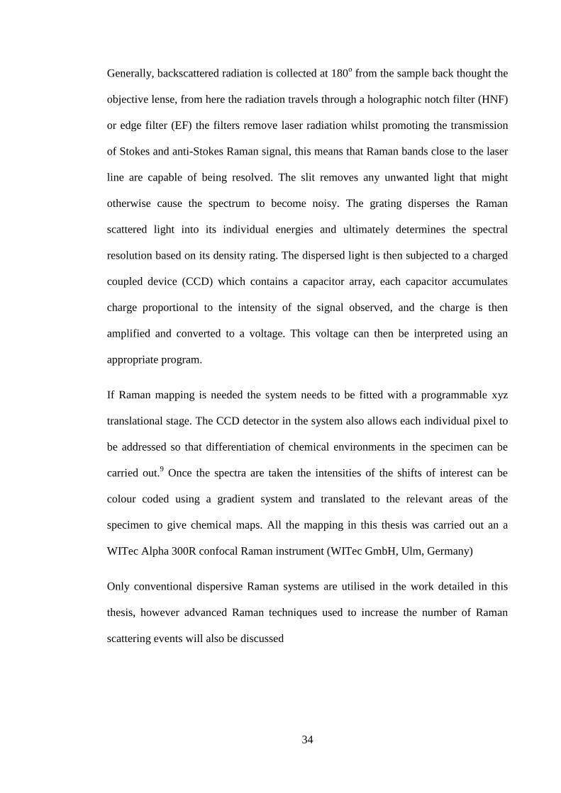
Figure 1.7 The schematic shows the internal components that make up the internal portion of the Raman spectrometer, the microscope and the
laser. The laser trajectory is represented by the red line and the back scattered radiation is represented by the blue line. The HNF could also be
replaced with an EF.
Page 36
36
1.5 Alternative Methods of Raman Spectroscopy
1.5.1 Non-Linear Raman Techniques
Conventional Raman Systems are described as linear techniques in which the single
photon event shows Raman scattering efficiency which is linearly dependent on the
laser power. When higher power densities are used and little photo-decomposition
occurs, it is possible that more than one photon may interact with the molecule at the
same time causing a multi-photon event, the intensity of which is not linearly related to
laser power.9 The non-linearity can be achieved by using either one or more lasers to
irradiate the sample at the same time. Two examples of non-linear Raman techniques;
Coherent anti-Stokes Raman Spectroscopy (CARS) and hyper Raman spectroscopy
(HRS) are discussed here.
1.5.1.1 Coherent Anti-Stokes Raman Spectroscopy (CARS)
CARS employs multiple photons to address the signature vibrations of a sample.
Typically three illumination sources are used. The first laser line creates a virtual state,
just as in ordinary Raman scattering. The second laser stimulates the formation of an
excited vibrational state by having a frequency that is equal to that which would be
scattered in spontanteous Stokes Raman scattering. The third laser then excites the
molecule to this second virtual state, emission of energy as the molecule relaxes back to
the ground state is called CARS.9 The mechanism is concerted as all the lasers operate
at the same time. The main advantage of CARS is that it can be used to study Raman
transitions in the presence of competing incoherent background radiation so is often
used in cellular Raman imaging.21,22,23,24
The diagrammatic representation of this
process is show in Figure 1.8.
Page 37
37
Figure 1.8 A diagrammatic representation of CARS, are the respective energies
of the photons emerging from the laser.
1.5.1.2 Hyper Raman Spectroscopy (HRS)
When a sample is illuminated with monochromatic radiation of an intense irradiance,
the scattered radiation exhibits frequencies approximate to Equation 1.13 displayed
below.25
Where represents the combined frequency of the two photons which
interact with the analyte and represents the change in the photons frequency.
(1.13)
This is usually achieved using a 1064 nm Nd:YAG laser.26
If sufficient power is present
it is possible that two photons can interact with the molecule at once causing the
creation of a virtual state at double the frequency of the laser excitation.9 It is the
relaxation from the excited virtual state to the ground state which is termed hyper
Raman Scattering (Figure 1.9). Employing a 1064 nm laser, results in fluorescence
being immediately reduced but scattering from the laser can be too low in frequency to
be detected by a CCD detector. The hyper Raman effect provides an efficient way of
Page 38
38
observing Raman scattering but the use of a high powered laser can be a disadvantage,
causing sample degradation.
Figure 1.9 A diagrammatic representation of hyper Raman scattering are the
respective energies of the photons emerging from the laser is the energy emitted
as the molecule relaxes from its virtual to ground state.
Page 39
39
1.6 Non-Instrumentational Techniques
There are a range of non-instrumental techniques that rely on the use of chemicals and
other species to bring about an observed Raman enhancement. Two such techniques are
resonance Raman scattering and SERS. The latter of the two is more important to this
report so will be discussed in much greater detail.
1.6.1 Resonance Raman Scattering
This method of Raman enhancement occurs when the frequency of the laser is close to
or matching the frequency of the molecular electronic transition. Scattering
enhancements of around 106 have been observed for this technique, but absorption of
laser light by a chromophore can often cause burning of the sample. In order to fully
understand how resonance Raman works it is necessary to address the Kramer
Heisenberg Dirac equation (KHD) which fully explains the effect that dependent factors
have on polarization. The KHD equation is displayed below in Equation 1.14, Where
is the molecular polarizability and and are the incident and scattered polarization
directions. Ʃ is the sum over all vibronic states of the molecue as might be expected
from the non-spectific nature of scattering. The remaining terms are constants. is the
ground vibronic state, a vibronic state of an excited electronic state and the final
vibronic state of the ground state. and represent the dipole operator of the incident
and scattered polarization direction, subscript represents the frequency change
between transitions. 9
( ) ∑(
⟨ | | ⟩⟨ | | ⟩
⟨ | | ⟩⟨ | | ⟩
)
(1.14)
Page 40
40
The equation is mathematically complex and its complete explanation is beyond the
scope of this thesis. However is should be understood that under resonance conditions
the denominator of Equation 1.14 becomes very small leading to the first term
becoming very large, resulting in an increased polarizability and much greater Raman
scattering.
1.7 Surface enhanced Raman spectroscopy (SERS)
As this thesis is concerned with the development and optimisation of SERS active
substrates and solution based systems it is essential that this area is addressed in detail.
SERS has become an area of great interest with the number of publications in the field
rising year after year.27,28
The attraction of SERS stems from the fact that it can be used
for a wide range of physical and biological applications.
1.7.1 Brief History
The SERS effect was first observed in 1974 by Fleischmann and co-workers.29
It was
identified that pyridine absorbed onto an electrochemically roughened silver surface
gave rise to intense Raman signals. The spectral enhancement was initially attributed to
the increased surface area of the roughened substrate. Approximately three years later in
1977 two groups Jeanmaire and Van Duyne30
and Albrecht and Creighton31
were the
first to ‘discover’ SERS and highlight the fact that the intensified Raman signals were
far in excess of the increased number of molecules interrogated as a result of the
surface’s roughness. In 1978 Moskovits proposed that the increased Raman cross
section was a result of plasmon excitations on the surface of the roughened silver32
and
this led to the development of the electromagnetic theory in the early 1980’s by
Gersten33,34
, Gersten and Nitzan35,36
, McCall et al37
and Kerker et al38
. Moskovits was
also able to approximate which metals would give the largest enhancement and thus
Page 41
41
hypothesise that the intense Raman cross section was not just confined to roughened
metal surfaces but could be replicated using metallic nanoparticles.39
Theories of
chemical enhancement were then established by Otto et al 40,41,42
in the late 1980’s. This
theory varied from the electromagnetic one in that the adsorbate had to bind with the
nanoparticles surface for increased enhancement to occur.
The interest in SERS was further increased in 1997 as work by Kniepp and co
workers43-46
and Nie and collegues47-50
highlighted that SERS could be used under
favourable conditions to detect single molecules. Conventional SERS has the ability to
increase Raman intensities up to 106 but single molecule surface enhanced Raman
scattering (SMSERS) has the ability to create enhancement factors above 1013
.
One of the more recent developments in the field include tip enhanced Raman
spectrscopy (TERS),51,52
this unites the two techniques, scanning near-field optical
microscopy (SNOM) and SERS, and is arguably one of the most intriguing
developments in optical microscopy. Here the tip of the AFM or STEM is silvered and
rastered across a substrates surface, this is carried out simultaneously with illumination
from a laser source. Not only is the substrates topography translated but its chemical
finger print is interpreted at the same time, giving high levels of spatial characterisation.
It must be remembered that SERS as a technique has been around for less than 40 years,
but developments in the field have been rapid. Even though the history is much more
involved than the brief outline given, it is essential that the mechanisms, theories,
synthesis and applications of SERS are addressed so that the effect can be fully
understood.
Page 42
42
1.8 Mechanisms of SERS
As mentioned previously, two mechanisms have evolved and proven to explain the
reason why metallic nanoparticles or roughened metallic surfaces give rise to an
increased Raman scattering cross section. These mechanisms are termed
electromagnetic and chemical.
1.8.1 The Electromagnetic Mechanism of SERS
The intensity of Raman scattering is dependent on the product of the polarizability
derivative and of the incident field intensity. The electromagnetic mechanism deals with
the effect that the surface plasmons of a metal have on increasing the incident field
intensity (e).53
Plasmons can be viewed in the same way as light, either in a wave form
or as a collection of oscillating quantized particles. The classical expression of plasmons
would be a collection of free electron gas oscillating at the surface of a dielectric
material.54
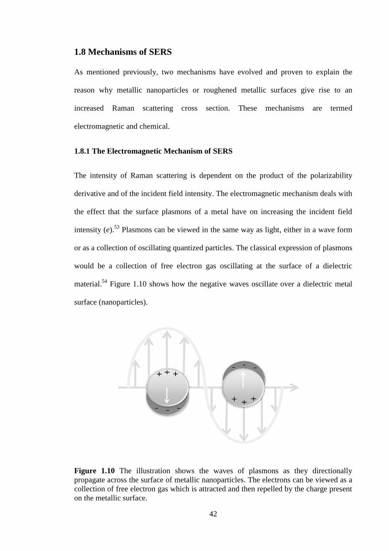
Figure 1.10 shows how the negative waves oscillate over a dielectric metal
surface (nanoparticles).
Figure 1.10 The illustration shows the waves of plasmons as they directionally
propagate across the surface of metallic nanoparticles. The electrons can be viewed as a
collection of free electron gas which is attracted and then repelled by the charge present
on the metallic surface.
Page 43
43
Most models of the electromagnetic SERS are based on the nanoparticles being
represented as small metallic spheres, however this is only a first approximation to a
colloidal arrangement and it is the collection of aggregated53
metallic spheres that give
rise to roughness in the system termed ‘SERS hotspots’.55
Electrodynamic experiments
allow the electromagnetic enhancement of metallic particles with different shapes and
sizes to be estimated. Most calculations find that the enhancement is less than 106 for a
single particle, but it can be seen that dimers or multi-nanoparticle systems give a much
greater enhancement53
here the increased electric field is found at the interface between
the nanoparticles and can be quantified using generalised Mie theory (GMT)
calculations. Mathematically the electromagnetic theory can be very complex and is
explained exceptionally well by Stockman56
but it is beyond the scope of this report to
delve into such difficult mathematics. Much easier mathematic expressions deal with
the nanoparticle as a singular spherical entity and can be seen below (Equation 1.15 and
1.16).
(
) (1.15)
is the total electric field at a distance from the spheres surface, is the radius of the
sphere, is the angle relative to the direction of the electric field and is the constant
related to the dielectric constant such that,
(
( (
) (1.16)
and represent the dielectric constants of the medium surrounding the sphere and of
the metal sphere respectively. is the frequency of the incident radiation. The value of
increases as the denominator decreases. When the denominator is at a minimum the
plasmon resonance frequency is increased causing the immediate area surrounding the
Page 44
44
nanoparticles to experience an increased local field energy this bathes the analyte in a
freely moving electron cloud. The electrons in the molecule then become polarized
giving rise to intense Raman scattering effects. The electromagnetic field is inversely
proportional to therefore the effect is greatest for analytes which are in close
proximity to the metallic nanoparticles.9 Although the electromagnetic effect accounts
for the greatest enhancement of Raman scattering it is only one theory.
1.8.2 The Chemical Mechanism of SERS
Chemical enhancement occurs when a bond is formed between an analyte and
nanoparticle. The bond allows communication between the species, so the transfer of
charge from the metals surface to the analyte can occur.57
The analyte comes into close
proximity to the surface of the nanoparticles and forms a bond. The part of the molecule
that binds to the surface is dependent on the functional groups present, generally
molecules which contain thiol groups will exhibit much stronger binding to gold
surfaces and molecules containing amines will bind strongly to silver.58
Once bound the
molecules experience electron cloud perturbation (polarization) due to the oscillating
free electrons which travel along the nanoparticles surface. Essentially electrons travel
up the metal-absorbate bond, interact with the absorbate causing polarization then the
electron returns back to the metals surface.9 This mechanism of enhancement can be
interpreted as a HOMO and LUMO interaction. Clearly the enhancement can only occur
up to monolayer coverage so the enhancement is limited by distance, however the effect
is well defined as a mode of enhancement and direct evidence exists for its presence in
SERS.59,60
Now the theories of SERS enhancement have been expressed, the nanoparticles which
are the main facilitators of this property should be explained.
Page 45
45
1.9 Nanoparticles and SERS Substrates
The nanoparticles are essentially dielectric materials, consisting of a positively charged
metal centre with sinusoidal electron waves sweeping across its surface as shown in
Figure 1.10. Synthesis of nanoparticles can take a conventional one-pot direction61,62
or
can be more complex using methods such as seeded-growth.63
Although metals such as
rhodium,64,65
platinum,66,67,68
ruthenium69
and copper70
have been shown to exhibit
SERS enhancement, SERS has almost exclusively been associated with silver and gold
nanoparticles because of the large enhancements these two coinage metals bestow. By
changing the size of the nanoparticles it is possible to control the plasmonic bands and
tailor the absorbance wavelength53
.
Shapes can also be varied using wet methods to tailor plasmon bands and although
spherical nanoparticles are most commonly used61,62
other shapes such as prisms,71
rods,72,73
star,74
and plates75-77
have also been synthesised. Much of the testing for SERS
activity of the nanoparticles involves the chemicals such as Rhodamine 6G, crystal
violet and 2-mercaptopyridine. Many of the papers use these chemicals because they
have been readily shown to give conformation of the SERS effect due to the
suppression of the fluorescence associated with dye molecules. Nanoparticle sols often
offer a better alternative to a thin film metallic surface because they have an increased
surface area and each singular nanoparticle is capable of acting as an area of localised
surface plasmon resonance. Nanoparticles in suspension also benefit from Brownian
motion and Raman spectra obtained from a solution represents an averaged effect.
However solid-state substrates are often used when dynamic problems such as degrees
of aggregation become a problem. The most common SERS substrates involve self-
Page 46
46
assembled layers of nanoparticles78
with other published articles outlining the use of
SERS surfaces use metallic island films as a SERS active surface.79-81
Chapters 2-5 in this thesis explore the use and synthesis of solid-state SERS substrates,
whilst 6-8 show the application of nanoparticles in solution-based systems. A more
comprehensive and specific introduction to their usage is given in each of the chapters
outlined.
Page 47
47
1.10 Aims and Objectives
The work contained in this thesis explores a variety of SERS applications. However, the
central theme is the ‘optimisation’ of SERS based systems in order to improve
reproducibility and enhancement effects for various different analytes of chemical and
biological significance. The main aims of which I hope this thesis addresses are:
The exploration of different methods for the synthesis of solid-state SERS
substrates.
The production of a substrate capable of competing with high-cost commercial
substrates.
The development of strategies for controlling the dynamics of solution based
SERS experiments.
The exploration of multiple data analysis techniques and their use in
disseminating important vibrational information from the interrogated samples
The application of SERS to the detection of significant chemical and biological
analytes.
Page 48
48
1.11 References
1. M. Heald and J. Marion, Classical Electromagnetic Radiation. Brooks Cole;
California, USA., 1994.
2. P. Atkins and J. D. Paula, Physical Chemistry. Oxford University Press; Oxford,
U.K., 2006.
3. C. N. Banwell, Fundamentals of Molecular Spectroscopy. McGraw-Hill,
Maidenhead, U.K., 1983.
4. D. C. Harris and M. D. Bertolucci, An Introduction to Vibrational and Electronic
Spectroscopy. Dover, New York, U.S.A., 1978.
5. J. J. Laserna, Modern Techniques in Raman Spectroscopy. John Wiley and
Sons; Chichester, U.K.., 1996.
6. M. Badino, Annalen Der Physik., 2009, 18, 81-101.
7. P. Atkins, Molecular Quantum Mechanics. Oxford University Press; Oxford,
U.K., 1999a.
8. J. Lakowicz, Principles of Fluorescence Spectroscopy. Plenum; New York,
U.S.A., 1999.
9. E. Smith and G. Dent, Modern Raman Spectroscopy: A Practical Approach.
John Wiley and Sons; Chichester, U.K., 2005.
10. N. Everall,, B. King and I. Clegg, The Raman Effect. Chemistry in Britain,
2000, 40-43.
11. S. P. Mulvaney and C. D. Keating, Analytical Chemistry., 2000, 72, 145-157.
12. P. Matousek, M. Towie, A. Stanley and A. W. Parker, Applied Spectroscopy.,
1999, 53, 1485-1489.
13. R. L. McCreery, Raman Spectroscopy for Chemical Analysis. Wiley
Interscience; Chichester, U.K., 2000.
14. S. Roy, W. D. Kulatilaka, S. V. Naik, N. M. Laurendeau, R. P. Lucht and J. R.
Gord, Applied Physics Letters., 2006, 89, 104-105.
15. D. A. Long, The Raman Effect. John Wiley and Sons; Chichester, U.K., 2002.
16. S. Koseki, T. Asada and T. Matsushita, Journal of Computational and
Theoretical Nanoscience., 2009, 6, 1352-1360.
17. J. R. Ferraro, K. Nakamoto and C. W. Brown, Introductory Raman
Spectroscopy. Elsevier Science; Oxford, U.K., 2002.
18. N. B. Colthup, L. H. Daly and S. E. Wiberley, Introduction to Infrared and
Raman Spectroscopy. Academic Press Limited; London, UK., 1990.
19. I. Degen, Tables of Characteristic Group Frequencies for the Interpretation of
Infrared and Raman Spectra. Acolyte publications; Harrow, U.K., 1997.
20. J. Twardowski and P. Anzenbacher, Raman and IR Spectroscopy in Biology and
Biochemistry, Ellis Horwood; New York, U.S.A., 1994.
21. C. L. Evans and X. S. Xie, Annual Review of Analytical Chemistry., 2008, 1,
883-909.
22. C. Krafft, B. Dietzek and J. Popp, Raman and CARS microspectroscopy of cells
and tissues. SPEC 2008 Conference on Shedding Light on Disease - Optical
Diagnosis for the New Millenium; Sao Jose dos Campos, Brazil, 1046-1057.
23. T. T. Le, T. B. Huff and J. X. Cheng, Cancer., 2009, 9, 14.
24. K. Fujita and N. I. Smith, Molecules and Cells., 2008, 26, 530-535.
25. L. D. Ziegler, Journal of Raman Spectroscopy., 1990, 21, 769-779.
26. D. V. Murphy, K. U. Vonraben, R. K. Chang and P. B. Dorain, Chemical
Physics Letters., 1982, 85, 43-47.
Page 49
49
27. R. Aroca, Surface-Enhanced Vibrational Spectroscopy. John Wiley and Sons;
Chichester, U.K., 2006.
28. D. Graham and R. Goodacre, Chemical Society Reviews., 2008, 37, 883-884.
29. M. Fleischmann, P. J. Hendra and A. J. McQuillan, Chemical Physics Letters.,
1974, 26, 163-166.
30. D. L. Jeanmaire and R. P. Van Duyne, Journal of Electroanalytical Chemistry.,
1977, 84, 1-20.
31. M. G. Albrecht and J. A. Creighton, Journal of the American Chemical Society.,
1977, 99, 5215-5217.
32. M. Moskovits, Journal of Chemical Physics., 1978, 69, 4159-4161.
33. J. I. Gersten, Journal of Chemical Physics., 1980, 72, 5779-5780.
34. J. I. Gersten, Journal of Chemical Physics., 1980, 72, 5780-5781.
35. J. I. Gersten and A. Nitzan, Journal of Chemical Physics., 1980, 73, 3023-3037.
36. J. I. Gersten and A. Nitzan, Journal of Chemical Physics., 1981, 75, 1139-1152.
37. S. L. McCall, P. M. Platzman and P. A. Wolff, Physics Letters A., 1980, 77,
381-383.
38. M. Kerker, Accounts of Chemical Research., 1984, 17, 271-277.
39. M. Moskovits, Surface-Enhanced Raman Spectroscopy: a Brief Perspective in
Surface-Enhanced Raman Scattering: Physics and Applications; Kneipp, K.,
Moskovits, M. and Kneipp, H. (Eds). Springer; Berlin, Germany., 2006.
40. I. Mrozek and A. Otto, Journal of Electron Spectroscopy and Related
Phenomena., 1990, 54, 895-911.
41. A. Otto, Journal of Raman Spectroscopy., 1991, 22, 743-752.
42. A. Otto, I. Mrozek, H. Grabhorn and W. Akemann, Journal of Physics-
Condensed Matter., 1992, 4, 1143-1212.
43. J. Kneipp, H. Kneipp and K. Kneipp, Chemical Society Reviews., 2008, 37,
1052-1060.
44. K. Kneipp, G. R. Harrison, S. R. Emory and S. M. Nie, Chimia., 1999, 53, 35-
37.
45. K. Kneipp and H. Kneipp, Biophysical Journal., 2005, 88, 365-365.
46. K. Kneipp, Y. Wang, H. Kneipp, L.T. Perelman, I. Itzkan, R. Dasari, R. and M.
S. Feld, Physical Review Letters., 1997, 78, 1667-1670.
47. W. E. Doering and S. M. Nie, Journal of Physical Chemistry B., 2002, 106, 311-
317.
48. S. R. Emory and S. M. Nie, Analytical Chemistry., 1997, 69, 2631-2635.
49. J. T. Krug, G. D. Wang, S. R. Emory and S. M. Nie, Journal of the American
Chemical Society., 1999, 121, 9208-9214.
50. S. M. Nie and S. R. Emory, Abstracts of Papers of the American Chemical
Society., 1997, 213, 177.
51. R. M. Stockle, Y. D. Suh, V. Deckert and R. Zenobi, Chemical Physics Letters.,
2000, 318, 131-136.
52. B. S. Yeo, J. Stadler, T. Schmid, R. Zenobi, and W. Zhang, Chemical Physics
Letters., 2009, 472, 1-13.
53. G. C. Shatz and R. P. Van Duyne, Electromagnetic Mechanism of Surface-
Enhanced Spectroscopy in Handbook of Vibrational Spectroscopy; J. M.
Chalmers and P. R. Griffiths (Eds). Wiley; New York, U.S.A., 2002, 759-774.
54. M. T. Michalewicz, Physical Review B., 1992, 45, 13664-13670.
55. R. C. Maher, M. Dalley, E. C. Le Ru, L. F. Cohen, P. G. Etchegoin, H.
Hartigan, R. J. C. Brown and M. J. T. Milton., Journal of Chemical Physics,
2004, 121, 8901-8910.
Page 50
50
56. M. I. Stockman, Electromagnetic theory of SERS in Surface-Enhanced Raman
Scattering: Physics and Applications; Kneipp, K., Moskovits, M. and Kneipp, H.
(Eds). Springer; Berlin, Germany., 2006.
57. H. Yamada, H. Nagata, K. Toba and Y. Nakao, Surface Science., 1987, 182,
269-286.
58. M. Winter, WebElements: the periodic table on the web, University of Sheffield
and WebElements, http://www.webelements.com.
59. Y. C. Liu, K. H. Yang and T. C. Hsu, Analytica Chimica Acta., 2009, 636, 13-
18.
60. S. M. Morton and L. Jensen, Journal of the American Chemical Society., 2009,
131, 4090-4098.
61. M. Brust, M. Walker, D. Bethell, D. J. Schiffrin and R. Whyman, Journal of
the Chemical Society-Chemical Communications., 1994, 801-802.
62. P. C. Lee and D. Meisel, The Journal of Physical Chemistry., 1982, 86, 3391-
3395.
63. E. Nalbant and A. Esenturk, A, Journal of Raman Spectroscopy., 2009, 40, 86-
91.
64. L. Cui, Z. Liu, S. Duan, D. Y. Wu, B. Ren, Z. Q. Tian and S. Z. Zou, Journal of
Physical Chemistry B., 2005, 109, 17597-17602.
65. B. Ren, X. F. Lin, J. W. Yan, B. W. Mao and Z. Q. Tian, Journal of Physical
Chemistry B., 2003, 107, 899-902.
66. M. A. Bryant, S. L. Joa and J. E. Pemberton, Langmuir., 1992, 8, 753-756.
67. P. G. Cao, Y. H. Sun and R. N. Gu, Journal of Physical Chemistry B., 2004,
108, 4716-4722.
68. J. Z. Zheng, B. Ren, D. Y. Wu and Z. Q. Tian, Journal of Electroanalytical
Chemistry., 2005, 574, 285-289.
69. B. Ren, X. F. Lin, Z. L. Yang, G. K. Liu, R. F. Aroca, B. W. Mao and Z. Q.
Tian, Journal of the American Chemical Society., 2003, 125, 9598-9599.
70. D. Y. Wu, X. M. Liu, S. Duan, X. Xu, B. Ren, S. H. Lin and Z. Q. Tian,.
Journal of Physical Chemistry C., 2008, 112, 4195-4204.
71. R. C. Jin, Y. W. Cao, C. A. Mirkin, K. L. Kelly, G. C. Schatz and Schatz and J.
G. Zheng, Science., 2001, 294, 1901-1903.
72. S. B. Chaney, S. Shanmukh, R. A. Dluhy and Y. P. Zhao, Applied Physics
Letters., 2005, 87.
73. T. Qiu, W. Zhang and P. K. Chu, Physica B: Condensed Matter., 2009, 404,
1523-1526.
74. C. G. Khoury and T. Vo-Dinh, Journal of Physical Chemistry C., 2008, 112,
18849-18859.
75. I. Pastoriza-Santos and L. M. Liz-Marzan, Journal of Materials Chemistry.,
2008, 18, 1724-1737.
76. Y. G. Sun and G. P. Wiederrecht, Small., 2007, 3, 1964-1975.
77. X. Q. Zou and S. J. Dong, Journal of Physical Chemistry B., 2006, 110, 21545-
21550.
78. M. Baia, F. Toderas, L. Baia, D. Maniu and S. Astilean, Chemphyschem, 2009,
10, 1106-1111.
79. L. L. Bao, S. M. Mahurin, C. D. Liang and S. Dai, Journal of Raman
Spectroscopy., 2003, 34, 394-398.
80. T. W. H. Oates, H. Sugirne and S. Noda,. Journal of Physical Chemistry C.,
2009, 113, 4820-4828.
81. H. Seki and M. R. Philpott, Journal of Chemical Physics., 1980, 73, 5376-5379.
Page 51
51
2. Preliminary Work on the Synthesis of Solid-
State SERS Active Substrates
Page 52
52
2.1 Abstract
This chapter outlines preliminary work on the synthesis of solid-state SERS substrates.
Initially attempts were made to synthesise substrates via the tethering of gold or silver
nanoparticles onto glass using either a polymer, poly(diallyldimethylammonium
chloride) or functionalized silane ((3-aminopropyl)triethoxysilane or (3-
mercaptopropyl)triethoxysilane). An alternate route that was investigated utilises
Tollen’s reagent to deposit silver nanoclusters onto aluminium foil. In order for the
substrates manufactured to be considered for usage in SERS analysis, it was essential
that they adhered to a number of criteria defined in the following introduction. It was
discovered that the nanoparticle tethering methods produced substrates that
demonstrated homogeneous deposition of nanoparticles with varying degrees of
aggregation across the glass surface, however when interrogated using Raman it
revealed that the substrate had significant background contributions thus making it
impractical for SERS analysis. Deposition of silver nanoclusters on the surface of the
foil was also successful, but pre-treatment of the aluminium with acid was essential to
provide seeding sites that promoted nanocluster growth. The random positions of the
erosion sites caused the nanoclusters to be unevenly spaced across the aluminium
surface, meaning that whilst the roughened structures are likely to provide large SERS
enhancement, the effect would be irreproducible across the substrate. This is a
characteristic which is undesirable from an analytical perspective. Even though the
substrates described here could not be used for SERS analysis they provided an
important insight into establishing criteria by which a high performance thin film
substrate should adhere. The work here initiated the investigation of alternative
synthetic methods to produce solid-state SERS active substrates.
Page 53
53
2.2 Introduction - Setting the Scene for Successful Solid-State SERS
Substrate Synthesis
It is important to highlight the initial synthetic strategies used to produce SERS active
substrates and also detail their pros and cons which allowed the work in the following
three chapters to be carried out.
Initially the task was to create a solid-state SERS active substrate that would enhance
the Raman scattering effect of a range of chemical analytes. It was important before
carrying out any syntheses that a number of criteria relating to the ‘ideal’ SERS
substrate and its performance was established, thus allowing the resultant surfaces to be
assessed. The criteria used to define a robust substrate are detailed below:
1. The substrates surface must be roughened and synthesised from either gold or
silver in order for them to produce a large SERS enhancement.
2. No matter what synthetic methods were employed to create the substrates, they
must not show significant background contributions in the Raman spectra as this
only serves to complicate analysis.
3. A compromise must be met between the signal enhancement of an analyte and
its reproducibility. Developing conditions to maximise both is often
difficult/impossible.
4. The synthesis should be easily replicated under regular lab conditions, allowing
the technique to be accessible to non-specialist groups.
5. The manufacture of the substrates should also be cheap and facile.
One of the most detailed routes to substrate preparation is the binding of either silver or
gold nanoparticles synthesised in solution to a solid support.1-4
This provided a starting
point for the first synthesis.
Page 54
54
2.3 Preliminary synthesis 1 – Nanoparticle Substrates
2.3.1 Materials
Chloroauric acid (HAuCl4, 99.9%), poly(diallyldimethylammonium chloride) solution
(PDDA, MW=200,000-350,000), silver nitrate (99.9999%), (3-aminopropyl)
triethoxysilane (APTES, C9H22O3NSi, 95%) , (3-mercaptopropyl) triethoxysilane
(MPTES, C9H22O3SSi, 95%), concentrated sulphuric acid, hydrogen peroxide (30% w/v
in H2O), hydrochloric acid and nitric acid were purchased from Sigma Aldrich (Sigma
Aldrich, Dorset, U.K.) and used as received. Glass microscope slides and trisodium
citrate (99%) were purchased from Fisher Chemicals (Fisher Scientific UK Ltd,
Loughborough, U.K.). Solvents used in the synthesis were of analytical grade, whilst
water was HPLC certified.
2.3.2 Methods
2.3.2.1 Synthesis of Nanoparticles
2.3.2.1.1 Glassware Preparation
All glassware used to synthesise silver or gold nanoparticles was cleaned with aqua
regia [nitric acid: hydrochloric acid (1:3) v/v] to remove any residual metals, then
thoroughly rinsed with 3 sequential cycles of acetone and water in order to remove any
residual organic contaminants. The glassware was dried under a stream of nitrogen.
2.3.2.1.2 Gold Nanoparticles
Gold nanoparticles were synthesised according to a protocol described by Turkevich et
al.5 100 mL of HAuCl4 solution (50 mg) was added to 850 mL of boiling water under
vigorous stirring. Once the solution had returned to a boil, 50 mL of 1% trisodium
Page 55
55
citrate was added. After 30 min of continuous boiling and stirring the gold nanoparticle
solution was left to cool.
2.3.2.1.3 Silver Nanoparticles
Silver nanoparticles were synthesised according to a methodology outlined by Lee and
Meisel.6 Silver nitrate (90 mg) was dissolved in 500 mL of water (45
oC). The solution
was stirred and heated until the temperature reached 98 oC at which point 10 mL of 1%
trisodium citrate was then added. The solution was maintained at 98 oC and stirred for a
further 60 min.
2.3.2.1.4 Binding the Nanoparticles to the Glass Support
Two methods were employed to tether the nanoparticles (gold and silver) to a glass
support, one involved the use of poly(diallyldimethylammonium chloride) (polymer
methodology)7,8
and the other using a thiol or amine functionalized silane; MPTES or
APTES respectively (chemical methodology).1-4
2.3.2.1.5 Polymer Methodology
All glassware was cleaned using aqua regia prior to the synthesis taking place.
Glass microscope slides were hydroxylated by soaking in piranha solution (80 oC) for
60 min. After treatment the slides were then cleaned with copious amounts of methanol
and dried under a stream of nitrogen. Careful handling was exercised to minimise
contact and avoid contamination of the surfaces, this was found to be imperative if
successful functionalization and nanoparticle binding was to occur. The use of
plasticware opposed to glass after the hydroxylation process was also adopted to
maximise polymer interaction with the glass slides.
Page 56
56
The cleaned slides were individually placed into Petri dishes to which 25 mL of 2%
aqueous solution of PDDA was added. The slides were left to soak for 12 h on a rocking
platform. After functionalization the slides were washed with copious amounts of water
to remove excess polymer, then separately inserted into 50 mL centrifuge tubes. 40 mL
of gold or silver sol was then added to each tube and the slides were submerged for 24
h. The nanoparticle functionalized surfaces (substrates) were then washed in water to
remove any unbound nanoparticles. The substrates were then dried using a stream of
nitrogen and kept in a nitrogen flushed centrifuge tube until needed. The nanoparticle
tethered substrates were stored for no longer than a day before they were used.
2.1.2.1.6 Chemical Methodology
The same process for glass cleaning and microscope slide silanization was carried out as
detailed previously
Hydroxylated slides were placed in 50 mL centrifuge tubes, which contained 40 mL of a
5% methanolic solution of either APTES or MPTES. The slides were left to soak for 24
h, removed and then washed with copious amounts of methanol to remove any residual
unbound silanes. The functionalized slides were then placed in new 50 mL centrifuge
tubes to which either gold or silver sols were added (40 mL). After 24 h the substrates
were washed with water, dried and kept in individual centrifuge tubes flushed with
nitrogen until needed. Again the substrates were stored for no longer than a day before
they were used.
Page 57
57
2.1.2.1.7 Unsuccessful Substrate Preparations
Unfortunately binding of the nanoparticles to the glass support proved unsuccessful
when using the MPTES tether. It is suspected that the chemical formed sulphur
crosslinks in solution limiting the number of thiol groups accessible for nanoparticle
interaction, and also hindering the silane interaction with the glass. Therefore, only
substrates involving the use of APTES and PDDA were further investigated.
The use of APTES to bind the silver nanoparticles to the glass surface also proved
unsuccessful, as the colloid crashed out of solution over the 24 h soaking period.
Shaking of the sol was also unable to re-disperse the nanoparticles.
For both unsuccessful preparations the ratios of silane:colloid were changed to no avail,
No visible colour change on the surface of the glass was observed, therefore further
analysis of these unsuccessful syntheses was not pursued.
By contrast two methods attempted did yield nanoparticles bound to glass. A general
outline of the successful synthesis of the nanoparticle bound substrates is given in
Scheme 2.1.
Page 58
58
Scheme 2.1 The process for the production of SERS substrates through the adherence
of nanoparticles to a glass slide is shown. The scheme details the hydroxylation,
functionalization via chemical (APTES) and polymer (PDDA) methods, then finishes
with nanoparticle adhesion to the surface.
Page 59
59
2.3.3 Results and Discussion
2.3.3.1 Nanoparticle Characterisation
The successful synthesis of gold and silver nanoparticles is accompanied by a colour
change of the sol (Figure 2.1). The formation of silver nanoparticles is signified by a
colour change of the starting solution from colourless to a milky green hue, whilst the
gold solution exhibits a transition from yellow to a deep red colour upon the formation
of nanoparticles. Although it can be seen by eye that the absorbance of the solution has
shifted during the synthesis, it is common practice to establish the λmax using UV-Vis
spectrophotometry.
Figure 2.1 Images of gold and silver nanoparticle sols. The red solution on the left is
representative of a gold nanoparticle presence in solution whilst the milky green
solution on the right signifies silver nanoparticle formation.
2.3.3.2 UV-visible (UV-vis) Absorption/Extinction Nanoparticle Characterisation
To ensure that the absorbance of the nanoparticles (gold and silver) was less than 1, the
sols were diluted 1 part in 9 parts water. The sample was transferred to a quartz cuvette
and placed in the sample holder of a Thermo Biomate 5 (Thermo Fisher Scientific Inc.,
Massachusetts, USA). Data was acquired over a wavelength range of 300-800 nm. The
gold sol was shown to have a surface plasmon band (λmax ) of 529 nm, whilst the silver
sol exhibited a λmax at 421 nm. Both plasmon bands were positioned as outlined in the
literature.5,6
Page 60
60
2.3.3.3 Transmission Electron Microscopy (TEM)
TEM allows the size and shape of the nanoparticles to be determined. Images of the
gold and silver nanoparticles were acquired using a FEI Tecnai 12 Twin transmission
electron microscope (FEI, Hillsboro, Oregan, USA) operating at 100 kV. 10 µL aliquots
of the sol were spotted onto parafilm, a copper grid was then placed on top of the
droplets surface. The grids were left for 10 min then removed. The grids containing the
nanoparticles were analysed once fully dried. The images acquired from the gold and
silver nanoparticles are displayed in Figure 2.2. ImageJ (National Institutes of Health,
USA) version 1.46r was used to process the images making it possible to calculate the
mean diameter of the nanoparticles and their respective standard deviations. The gold
nanoparticles were estimated to have an average diameter of 25±14 nm, whilst the silver
nanoparticles were harder to process due to their differing aspect ratios. However, the
estimated average diameter was 90±70 nm.
Figure 2.2 TEM micrographs of the gold (top row) and silver (bottom row)
nanoparticles synthesised using citrate reduction. Scale bars are inset. The top row of
images have 100 nm and 50 nm scale bars (left and right respectively), whilst the scale
bars in the bottom row are both 200 nm.
Page 61
61
2.3.3.4 Characterisation of the Nanoparticles Bound to the Glass Substrate.
It was evident upon simple visible observation of the nanoparticle functionalized glass
slides whether the adhesion of silver or gold nanoparticles had been successful.
Depending on whether gold or silver nanoparticles were used the slides appeared red or
yellow respectively. Figure 2.3 shows some example slides exhibiting successful
functionalization using gold and silver nanoparticles.
Figure 2.3 The images show glass slides functionalized with gold nanoparticles (left)
and silver nanoparticles (right).The gold functionalized surface exhibits a light red
colour whilst the silver surface appears yellow.
2.3.3.5 Scanning electron microscopy (SEM)
SEM images were acquired for all the substrates that were successfully synthesised.
Samples were however prepared on a silicon substrate, which helps to disperse negative
charge and provides a greater contrast than glass thus resulting in higher resolution
images and the reduction of noise. The use of silicon mimics glass so the nanoparticle
depositionis comparable. Micrographs were collected using a Zeiss Supra 40 VP field-
emission gun scanning electron microscope (FEG-SEM; Carl Zeiss SMT GmBH,
Oberkochen, Germany) operating at a voltage of 1 kV. The images taken from the
substrates at different magnifications can be seen in Figure 2.4. It can clearly be seen
that in all preparations the nanoparticles are homogeneously deposited across the
surface. Formation of agglomerated nanoparticles on the polymer bound silver substrate
Page 62
62
can be seen more frequently than on the gold substrates, the nanoparticle clusters
signify the potential position of SERS ‘hotspots’, however the random positioning of
sites means that there could be significant variation in the SERS signal produced
whenan analyte interacts with the silver. A similar aggregation of nanoparticles can be
seen when gold is bound to the glass using the polymer, except in this case the clusters
formed appear to contain between 2-8 nanoparticles. The gold nanoparticles bound to
the support using APTES demonstrate minimal clustering with the particles being
mono-dispersed across the surface. The aminosilane binding directly contrasts the
polymer binding in that little or no aggregation is observed. The mono-dispersity of the
nanoparticles may ensure a more reproducible SERS signal, but the lack of aggregation
may severely hamper the degree of Raman enhancement. Ideally a SERS substrate
would consist of nanoparticle clusters, with the same numbers of nanoparticles present
in each aggregate. The clusters should be homogeneously spread across the substrate so
that reproducibility of large enhancement factors is realised. At this stage the substrate
which adheres most to this criteria is the PDDA tethered Au preparation.
The next step was to scrutinise the SERS activity of the substrates.
Page 63
63
Figure 2.4 The SEM images show the gold and silver nanoparticles bound the silicon
support. The top row shows silver nanoparticles tethered using PDDA, the middle row
shows gold nanoparticles bound using PDDA and the bottom row shows gold
nanoparticles attached using APTES. The scale bars and magnification are inset in each
of the images.
Page 64
64
2.3.3.6 Raman Analysis
Spectra were collected using a WITec Alpha 300R confocal Raman instrument (WITec
GmbH, Ulm Germany). The substrates were interrogated using a laser wavelength of
632.8 nm with an unfocussed power of 1mW. The density of the grating coupled to a
thermoelectrically cooled charge coupled device (CCD) was 600 g mm-1
. Spectra were
collected between 500- 2840 cm-1
, using an Olympus 50x/0.5 objective. A total of 20
spectra were obtained from random areas on each substrate. A single spectrum
acquisition time of 1 s was used.
Spectra were first collected from the blank colloidal substrates (Figure 2.5). It can be
seen that each substrate has significant background spectra, regardless of the metallic
composition of the nanoparticles or the method used to adhere them to the glass slide.
The background spectra generated on each of the surfaces appears to arise from a
combination of both citrate and binding/tethering agent scattering. Peaks at 814, 942,
1030, 1369 and 1643 cm-1
are relatively consistent across all three substrates so are
most likely to represent the citrates which were used to stabilise the nanoparticles. The
polymer substrates display common peaks across the wavenumber range of 1100 – 1570
cm-1
, whilst the silane substrates exhibit two discrete peaks at 1875 and 2089 cm-1
. The
presence of vibrational bands arising from the blank substrates is detrimental to SERS
analysis as scattering from analytes applied to the surface may overlap with the
background peaks or be masked completely. Based on the high degree of scattering
from the blanks it was decided that these substrates were not ideal, so further analysis
was abandoned and new methodologies pursued.
Page 65
65
Figure 2.5 The staggered spectra are representative of the 3 colloidal substrates synthesised using PDDA (polymer) or APTES (silane) tethering
agents. The red and blue spectra represent Ag and Au nanoparticles tethered using PDDA respectively. The black spectrum represents Au
tethered using APTES.
Page 66
66
2.4 Preliminary Synthesis 2 –Silver Nanoclusters deposited on
Aluminium Foil
2.4.1 Materials
Silver nitrate (AgNO3, 99.9999%), ammonia solution (NH4OH, 30% w/v), hydrochloric
acid and glucose were purchased from Sigma Aldrich (Sigma Aldrich, Dorset, U.K.).
Aluminium foil was purchased from a high street retailer. All reagents were used as
supplied. Any solvents used in the synthesis of the substrates were analytical grade and
the water used was HPLC certified.
2.4.2 Methods
2.4.2.1 Substrate Synthesis
The method of preparation is adapted from Yi He et al.9
In a typical synthesis
aluminium foil was wrapped around a 96 well plate and smoothed into the wells. This
created a semi-circular indentation into which the silver solution could be spotted. The
wells were cleaned with water and acetone before being treated with HCl (1 M) for 5
min. The acid treated wells were then washed using copious amounts of water and dried
under a stream of nitrogen. The reactive silver solution was formed by adding ammonia
dropwise to 10 mL of aqueous silver nitrate solution (0.12 M) until the brown AgOH
precipitate just disappeared. The newly formed Ag(NH3)2OH solution was mixed with
15.0 mL of aqueous glucose (0.56 M). The reaction solution was vortexed for 3 s then
immediately spotted in 25 μL aliquots into the pre-treated aluminium wells and left for
60 min. After deposition the silver targets were rinsed with water and dried under a
stream of nitrogen.
Page 67
67
2.4.3 Results and Discussion
2.4.3.1 Characterisation of the Aluminium Foil Substrates
Characterisation of the substrates was carried out using a Zeiss Supra 40 VP field-
emission gun scanning electron microscope operating at a voltage of 10 kV. A solitary
silver nanocluster is shown in Figure 2.6. Silver nanosheets which make up the
nanoclusters appear to grow perpendicular to the Al foil surface. The average diameter
of the clusters is estimated to be 3.5±0.5 µm, whilst the silver sheets from which the
clusters are constructed have a width of 10±2 nm.
Figure 2.6 The SEM image displays a single 2D silver nanocluster composed of silver
nanosheets which has been synthesised on Al foil. The nanocluster is 3 µM in diameter.
It is evident from Figure 2.7, that the acid erosion sites play an important role in seeding
the formation of the nanosheets from which the clusters are comprised.
Page 68
68
Figure 2.7 The image shows that the favourable sites for nanoplate formations are in
the crevices created by acid erosion. The image shows that not only are single deposits
formed but also groupings of deposits due to seeding. Scale bar and magnification
values are inset.
In the soft alkaline medium (~pH 10) the silver ammonium ion is reduced to silver
depositing the nanosheets at the surface of the aluminium.
The formation of the substrate can be summarized using the equation:
Al (s) + 3[Ag(NH3)2]+ (aq) + 3H2O (l) Al(OH)3 (s) + 3Ag (s) + 3NH3 (aq) + 3NH4
+ (aq)
Figure 2.8 shows that the silver clusters are not homogeneously dispersed across the
entire aluminium surface and that some areas are much more densely populated with
nanoclusters than others. Closer inspection of the substrates reveal that the patchy
spread of silver deposits is caused by the irregular pattern of acid erosion sites on the
foil. Whilst it is expected that the roughened deposits will give rise to large
enhancement factors, the uneven distribution of the nanoclusters is detrimental to the
production of a reproducible enhancement across the substrates surface. Here it is
obvious that the acid erosion forms important seeding sites for the nanostructures
Page 69
69
growth, unfortunately controlling homogenous erosion across the substrate is difficult
and one factor which could not be controlled here.
Figure 2.8 The SEM image shows that the nanocluster deposits are denser in some
areas compared to others. The image also shows that some areas of the aluminium have
no silver nanocluster coverage at all.
2.5 Conclusion
The substrates synthesised here do not adhere to the initial criteria outlined above for
the production of a suitable SERS thin film substrate. However, they have provided an
important insight into factors which are detrimental in the creation of a successful and
robust solid-state SERS substrate. New strategies to produce substrates will not involve
the use of tethering agents, because the Raman scattering of these chemicals can also be
enhanced by the bound nanoparticles. It is also important that silver or gold deposited
on a support is homogeneously spread across the surface. One methodology for the
production of SERS substrates which is explored in the next 3 chapters is galvanic
displacement of silver onto a copper support.
Page 70
70
2.6 References
1. G. Festag, A. Steinbrück, A. Wolff, A. Czaki, R. Möller and W. Fritzche,
Journal of Fluorescence, 2005, 15, 161-170.
2. V. Shakila and K. Pandian, Journal of Solid State Electrochemistry, 2007, 11,
296-302.
3. O. Seitz, M. M. Chemime, E. Cabet-Deliry, S. Truong, N. Felid, C. Perrinchat,
S. J. Grenes, J. F. Watts, Colloids and Surfaces A: Physiochemical and
Engineering Aspects, 2003, 218, 225-239.
4. M. Fan and G. Brolo, Physical Chemistry Chemical Physics, 2009, 11, 7387-
7389
5. J. Turkevich, P. C. Stevenson, J. Hillier, Discussions of the Faraday Society,
1951, 11, 55-75.
6. P. C. Lee and D. Meisel, The Journal of Physical Chemistry, 1982, 86, 3391-
3395.
7. W. Ji, X. Xue, W. Ruan, C. Wong, W. Ji, L. Chen, Z. Li, W. Song, B. Zhao and
J. R. Lombardi, Chemical Communications, 2011, 47, 2426-2428.
8. J. Xiao, F. Zhang, R. Li, Y Meng and W. Wen, Applied Spectroscopy, 2012, 66,
240-253.
9. Y. He, X. Wu, G. Lu and G. Shi, Nanotechnology, 2005, 16, 791-796
Page 71
71
3. The Optimisation of Facile Substrates for
Surface Enhanced Raman Scattering through
Galvanic Replacement of Silver onto Copper.
Published in Analyst. (Hot Article)
Contributing authors and their roles:
Iain Larmour2: Helped with the Raman instrument set-up and substrate interrogation
Vladimir Vishnyakov3: Collected the SEM images
Yun Xu1: Contributed to the morphological scores analysis
Duncan Graham2: Provided access to the Raman instrumentation
Royston Goodacre1: Principal Investigator
1 Manchester Interdisciplinary Biocentre, School of Chemistry, University of
Manchester, 131 Princess Street, Manchester, UK.
2 Centre for Molecular Nanometrology, WestCHEM, Department of Pure and Applied
Chemistry, University of Strathclyde, 295 Cathedral Street, Glasgow, UK.
3 Surface Coating and Characterisation Research Group, Department of Chemistry and
Materials, Manchester Metropolitan University, Chester Street, Manchester, UK.
Page 72
72
3.1 Abstract
A fast and cost-effective approach for the synthesis of substrates used in surface
enhanced Raman scattering (SERS) has been developed using galvanic displacement.
Deposition of AgNO3 onto commercially available Cu foil has resulted in the formation
of multiple hierarchical structures, whose morphology show dependence on deposition
time and temperature. Analysis of the surface structure by scanning electron microscopy
revealed that the more complex silver structures correlated well with increased
deposition time and temperature. Using Rhodamine 6G (R6G) as a model Raman probe
it was also possible to relate the substrate morphology directly with subsequent SERS
intensity from the R6G analyte as well as the reproducibility across a total of 15
replicate Raman maps (20*20 pixels) consisting of 400 spectra at a R6G concentration
of 10-4
M. The substrate with the highest reproducibility was then used to explore the
limit of detection and this compared very favourably will colloidal-based SERS
assessments of the same analyte.
Page 73
73
3.2 Introduction
An increasing amount of interest is being invested in the development of metallic
nanostructures due to their potential applications in catalysis, biomedicine, information
storage and sensing.1-5
Coinage metals such as copper, gold and silver have shown a
huge amount of potential and are useful in ultra-trace biological and chemical sensing,
surface plasmon resonance (SPR) and surface enhanced Raman scattering (SERS). 6-10
A substantial amount of time and effort has also been centred on the modification of
synthetic strategies that provide the desired control over nanostructure morphology.
Commonly applied methods of synthesis include photochemical reactions,11
use of
templates,12
seed-mediated growth,13
electrochemical deposition,14,15
Ultrasonic-assisted
template methods16,17
and surfactant/organic molecule assisted
reduction/stabilisation.18,19
Development of these methodologies has allowed the
creation of nano-metallic rods,20,21
chains,22
cubes,23
wires,24
plates,25
spheres,26
stars27
and dendrites.28
. However many of the synthetic techniques are either labour intensive
and/or necessitate the use of expensive instrumentation. Two highly desirable properties
of SERS substrates are the creation of areas of high enhancement with the concomitant
ability to tune the localised surface plasmon resonance of the nanostructures. A readily
accessible technique that can achieve this is galvanic displacement (GD)29-31
which also
offers the option of nanostructural growth on an appropriate substance in an extremely
efficient, facile and rapid way. This electroless plating technique has been reported for
Au on Si, Cu on Si, Zn on Al and multiple other combinations.32-34
Our focus of
galvanising Cu using Ag has very recently been reported and the resultant structures
from this readily accessible synthesis have been suggested as an effective process for
the production of SERS substrates.35-36
.
Page 74
74
As a result of the difference in electric potentials between the silver solution and copper
foil, deposition can occur very quickly, which although promoting anisotopic growth is
favourable in the development of a SERS substrate because of increased particle
aggregation and hence, the formation of high enhancement areas. Another aspect of GD
which is favourable for SERS is the ability to tune the nanostructures’ optical
properties. The origin of these properties is a phenomenon known as localised surface
plasmon resonance (LSPR). When these roughened metal surfaces are irradiated with
light delocalised electrons (plasmons) collectively oscillate relative to the lattice of
positive nuclei and couple to the photon to create a new quasi-particle known as a
plasmon polariton29
. For the coupling to occur it is essential that the plasmons oscillate
at a frequency which is close to that of the incident light. It has been demonstrated that
shape and geometry controlled synthesis of these nanostructures is a versatile route in
the tuning of the LSPR peak position across the visible and NIR spectral regions29
. In
much of the earlier work on silver or gold substrates, fabrication has involved the
immobilisation of colloidal nanoparticles onto solid platforms such as glass or quartz.
These metals are often bound to the surface via a functionalized silane linker or
polymer37,38
. Apart from the syntheses of these substrates being laborious, signals from
the organic molecules used in the linking or reduction/stabilisation of the nanoparticles
can repeatedly result in the existence of background signal, making the spectral
signature of the analyte very difficult to resolve. Furthermore the bound nanoparticles
are predominantly mono-dispersed which obviates extra signal enhancements obtained
at nanoparticle interfaces. Here we have exploited the difference in electrode potentials
to fabricate substrates in which the Ag+ ions have spontaneously replaced Cu atoms
through GD. For the reaction to proceed the metal with the higher electode potential
must be in solution. In our case Ag+/Ag possesses a potential of +0.799 V (SHE)
Page 75
75
whereas Cu2+
/Cu has a potential of +0.337 V (SHE) so the AgNO3 is contained in
solution. The full and half equations for this reaction are displayed in Scheme 3.1.
Scheme 3.1 The galvanic displacement of silver solution onto copper proceeds
according to the redox reaction displayed. The silver is in solution because the electrode
potential of the metal is more positive than that of the copper. It is essential that the
reaction is constructed in this way for deposition to proceed.
Differences in the structure of the silver surface can be produced by modifying the
concentration of the silver solution, heating the solution or changing the deposition
time. This can also have a profound effect on the enhancement of the Raman signal
arising from the analyte. As concentration effects have been extensively explored our
focus is on how the alteration of deposition time and temperature affects the
reproducibility and enhancement of Rhodamine 6G (R6G). The probe analyte R6G has
been chosen because of its problematic fluorescence in the absence of a SERS substrate
and its widespread use in SERS as a test anayte.39
Much of the past optimisation work
has revolved around the theorisation of synthetic strategies to produce surfaces with the
best SERS response, here optimisation is carried out on the basis of spectroscopic
results, which are presented in an unbiased and raw manner.
Page 76
76
3.3 Experimental
3.3.1 Materials
Silver nitrate (99.9999%), Rhodamine 6G and trisodium citrate were purchased from
Sigma Aldrich (Dorset, U.K.). Copper foil (1mm thickness) was obtained from a
commercial retailer. All solvents used throughout the synthesis were of analytical grade
and water was HPLC certified.
3.3.2 Methods
3.3.2.1 Synthesis of Optimal Silver on Copper (SoC) Surface
Copper foil was cut into 2.5 cm x 7.5 cm strips and fixed to a standard microscope slide
to generate a more rigid surface. The Cu surface was then cleaned with copious
amounts of methanol followed by acetone. 10 μL of 0.1M AgNO3 solution was then
spotted onto the surface and left to develop for a specified time. Deposition of the
nanoparticles was signified by the formation of a grey target on the copper foil. Post
deposition, further surface cleaning was carried out using deionised water to remove
any residual silver nitrate reagent and copper nitrate product. The substrate was then
dried under a stream of nitrogen.
3.3.2.2 Synthesis of Silver Nanoparticles
All glassware was cleaned using aqua regia [nitric acid:hydrochloric acid (1:3, v/v)] this
was performed to remove any trace metals, which may be residing in the glassware.
After an hour of treatment the flasks were then scrubbed with soap and rinsed with
water. The flasks were then left to dry in a 50oC oven for 20 min. Silver nanoparticles
were synthesised using the Lee and Meisel method.40
Briefly, AgNO3 (90 mg) was
dissolved in 500 mL of water and brought to the boil. A solution of 1% trisodium citrate
Page 77
77
(10 mL) was added. The solution was then left on a steady boil for 1 h. The reaction
was deemed to have reached its end point once the solution had a milky green hue.
3.3.2.3 UV-visible (UV-vis) Absorption/Extinction Characterisation of
Nanoparticles
Silver nanoparticles synthesised by citrate reduction where characterised using UV-
visible spectroscopy to determine the surface plasmon band λmax of the nanoparticles.
In order for the absorbance values to be less than 1 it was necessary to dilute the sol 1
part in 9 parts water. 1 mL of the diluted nanoparticle solution was then placed into a
quartz cuvette and inserted into the sample holder of a Thermo Biomate 5 (Thermo
Fisher Scientific Inc., Massachusetts, USA). An absorbance spectrum was collected
over a range of 300 to 800 nm. The silver sol was shown to have a surface plasmon
band λmax of 421 nm, which is characteristic of silver colloids synthesisedusing the Lee
and Meisel method.41
3.3.2.4 Scanning electron microscopic (SEM) and Energy Dispersive X-ray
Analysis (EDX)
SEM allows for the accurate determination of nanoparticles size and shape distributions
in a sol and also helps in the tracking of morphological changes at the copper/silver
interface created using GD. For the imaging of nanoparticles synthesised in solution, 10
μL of the sol was spotted onto a silicon slide and left to dry for 24 h. Microscopic
analysis of the SoC slides was carried out on the silver targets deposited as described in
the synthesis. SEM analysis of the SoC substrates was carried out using a Zeiss Supra
40 VP field-emission gun scanning electron microscope (FEG-SEM; Carl Zeiss SMT
Page 78
78
GmBH, Oberkochen, Germany) operating at a voltage of 3 kV, imaging of the silver sol
was carried out at a voltage of 1 kV. The SEM is also equipped with an EDX instrument
(EDAX Inc., New Jersey, USA) which was used to identify the elemental composition
of selected substrates. Here EDX was used to verify that silver had been deposited onto
the copper surface.
3.3.2.5 Preparation of SoC Substrates for Raman Mapping
For the exploration of temporal effects on the silver deposition and relative analyte
signal, the length at which the silver solution was applied to the surface for was altered.
Effects of deposition time where examined at 10 s, 20 s and 30 s. Once the optimum
deposition period had been identified it was then used to explore temperature effects.
Silver nitrate was spotted onto the copper surface at room temperature (RT=~23 oC), 30
oC, 40
oC, 50
oC, 60
oC, 70
oC, 80
oC, 90
oC and 100
oC. For the Raman optimisation of
the substrates 1 μL of a 10-4
M methanolic R6G solution was spotted onto the silver
deposition site and left to air dry. Once the most reproducible substrate had been
identified it was used to establish the limit of detection of R6G.
3.3.2.6 Raman Mapping
Raman analyses were undertaken using a WITec Alpha 300R confocal Raman
instrument (WITec GmbH, Ulm Germany) fitted with a piezo-driven XYZ scan stage.
All samples were probed using a laser wavelength of 632.8 nm. The grating was 600 g
mm-1
and coupled to a thermoelectrically cooled charge-coupled device (CCD). A
spectral resolution of 2.7 cm-1
was achieved over a spectral width consisting of 1024
Page 79
79
pixels spanning from 130-2900 cm-1
. The unfocussed laser power at the sample was
measured at ~1.0 mW. Spectra were acquired across an area measuring 20 μm x 20 μm
using an Olympus 50x/0.5 objective. 20 points per line and 20 lines per image were
recorded to give a spatial resolution of 1 μm. Each spectrum had an integration time of
0.08 s. Five replicate maps were taken on each of the three substrates, resulting in 15
maps being obtained at each optimisation parameter. Background spectra of all the
synthesised silver targets were acquired before maps were collected on the R6G
deposited surfaces. All data used in the analysis were collected from in and around the
silver targets centre to avoid any data discrepancies that could occur from mapping at
the areas at the target edges. In order to show that the enhancement was purely obtained
from the silver target one exemplar map has been generated at silver deposition area and
copper interface (see discussion below).
3.3.2.7 Colloidal-Based SERS in Solution
Spectra were collected using a DeltaNu Advantage benchtop Raman spectrometer
(Intevac inc, California, U.S.A.). The instrument is equipped with a 633 nm HeNe laser
with a power output of 3 mW. Spectra were collected for 5 s over a range of 200-3400
cm-1
at a spectral resolution of 10 cm-1
. Solution samples were placed in an 8 mm
diameter glass vial and subjected to laser irradiation once loaded into the sample cell
attachment. The instrument was calibrated to determine the ideal distance from the laser
to the glass vial using toluene and polystyrene. In a typical SERS interrogation 200 μL
of aqueous R6G was added to 200 μL of silver sol along with 50 μL of 0.5M KNO3
aggregating agent. The vial was then vortexed for 5 s and inserted into the sample cell
attachment where a spectrum was acquired immediately.
Page 80
80
3.4 Results and Discussion
3.4.1 Characterisation of Substrates
During galvanic displacement it was observed that the silver nanocrystals deposited on
the surface of the copper display an array of morphologies that appeared to be
dependent on deposition time and temperature. In Figure 3.1, the representative SEM
images show a selection of these deposits where it can be observed that when the silver
nitrate solution was left to develop for longer time periods on the surface of the copper
the more elaborate the deposition morphologies became. The blank copper surface can
be seen to be fairly smooth with only a few sites on the surface displaying indentations
or roughness. The galvanic displacement reaction takes place extremely quickly, so
when the silver nitrate solution was applied onto the surface for only 10 s there was an
appreciable deposition and growth of silver nanocrystals across the copper. A maximum
deposition time of 30 s was chosen because of the difficulty in washing off any excess
silver nitrate or newly formed copper nitrate solution without removing the silver
crystals from the copper. At 30 s the size of the silver deposits increases rapidly and the
morphologies differ greatly. Crystalline deposits with diameters of ~2 μm were
observed at 30 s deposition time as well as dendritic deposits and nanoparticle clusters.
Spotting of the AgNO3 solution on the copper surface at differing temperatures also
yielded varying effects. As the temperature was increased so did the complexity of the
silver deposits. When the silver was applied at RT only single and clustered
nanoparticles were formed. At a mid-range temperature
Page 81
81
Figure 3.1 SEM images taken of the silver on copper (SoC) substrate at a range of
deposition times and temperatures. The top row of images show the blank copper
surface and the surface after silver nitrate deposition times of 10 s and 30 s at toom
temperature (RT~23oC). The temporal evolution of the substrate shows more complex
structure formation occurs when the silver nitrate is left to mature on the surface for
longer time periods. The image taken after 30 s of GD time show the formation of large
nanoparticles, nanoplates and dendrites. The bottom row of SEM images display the
effect of deposition temperature on the morphology of silver on the surface of the
copper. At RT silver nanocrystals are formed on the copper surface and show a great
affinity for clustering at 60oC the clustering of the silver particles is still present
however, there is also evidence for the formation of nanoplates and dendrites. By
contrast at 100oC the surface solely consists of dendritic silver structure.
of 60oC bigger crystalline deposits could be observed along with the initial formation of
dendrites as observed when the deposition was carried out at RT for 30 s. By contrast, at
the maximum deposition temperature of 100oC the surface was completely covered in
the silver dendritic structures. It can be concluded from these SEM images (and the
replicate surfaces under the same conditions also showed this effect; data not shown)
that the growth of silver deposits at the copper interface is anisotropic with extremes of
temperature or time inducing the growth of much more heterogeneous and complex
structures. The formation of Ag dendrites has previously been observed in galvanic
displacement-type reactions and the diffusion limited aggregation model justifies their
synthesis.42
Previously it has also been shown that trunks and branches grow along the
Page 82
82
<211> directions and the leaves grow along <111> direction of the cubic Fm3m
structure, leading to the formation of dendrites.43
To investigate the coverage of silver on the surface at a variety of experimental
temperatures and times, energy dispersive X-ray analysis was carried out. The results of
the EDX analyses are summarised in Table 3.1. Although it is not possible to derive
clear compositional data from EDX analysis it can be revealed that the particles, plates
and dendritic structures which appear at the target sites are indeed composed of silver.
No great variation in the elemental composition of the substrate was observed. The
surface that was synthesised for 30 s at RT shows a slight drop in the % Ag and an
increase in % Cu but as previously discussed this could be due to silver mass lost
through the washing cycle. The low % O weight at the surface is also promising as
oxidation of the silver nanostructures has been shown to hinder SERS.44
Weight of Elements (%)
Variation of Deposition Time and Temperature Ag Cu O
20 s, RT 36.7 62.0 1.3
30 s, RT 32.5 65.0 2.4
20 s, 100oC 36.9 61.8 1.3
Table 3.1 Estimates of elemental composition from EDX analysis for the SoC
substrates.
Page 83
83
3.4.2 Proof of SERS Activity
To demonstrate that the SERS effect was only arising from the silver surface R6G
(1x10⁻⁴
M) was spotted across the silver/copper interface and mapped. The mapping
parameters used were as described previously except the area mapped was extended to
80 μm x 80 μm. The optical image, heat map and Raman spectra representative of
signals arising from the silver and copper surface are shown in Figure 3.2. The optical
image clearly defines the interface between the silver deposition site (red dot) and
copper surface (blue dot). The heat map was generated using the baseline corrected
peak area of the R6G peak at 1368 cm-1
, which is characteristic of the combined C-C
and C-N stretches (Table 3.2). The signal at 1368 cm-1
is only visible on the surface
where the silver has been deposited and not on the copper, thus proving that the GD of
silver is SERS active, and that smooth Cu is not generating any SERS effect. The
spectra show an average of 10 random spectra taken from in and around the areas
represented by the red and blue dots, these reinforce the fact that signal only arises from
the R6G which is present on the silver target whilst the spectra acquired from sites on
the copper display background noise only.
Page 84
84
Figure 3.2 (A) Optical image showing the area on the border of the silver deposition
area (red dot) and copper that was mapped (blue dot). (B) Corresponding heat map
generated by integrating under the R6G peak present at 1368 cm-1
. The spectrum
displayed in C is representative of Rhodamine 6G spectra acquired on the silver surface,
whilst spectrum D represents spectra acquired on the background copper surface. Both
C and D are the direct result of averaging 10 spectra taken from the areas highlighted by
the red and blue dots.
Page 85
85
3.4.3 Optimisation of Deposition Time
To generate substantial and comparable data sets three replicate SoC substrates were
produced at each time point (9 targets in total). Once synthesised R6G was applied
immediately to each of the surfaces; generally the time between the substrate being
synthesised and the conclusion of the Raman mapping was around 1 h. The intensity
values for each of the 400 spectra and the Raman shift values present in each map were
extracted using the WITec software. The 45 maps were then individually imported into
Matlab (MathWorks, Cambridge, U.K.) and reshaped to represent a data matrix whose
rows and columns consisted of data points and Raman intensity respectively. Plots of
the raw R6G spectra were visualised and six characteristic R6G peaks were selected at
619 cm-1
, 778 cm-1
, 1324 cm-1
, 1368 cm-1
, 1513 cm-1
and 1650 cm-1
for further scrutiny.
Table 3.2 shows the peaks and their archetypal vibrations that were selected for analysis
and Figure 3.3 demonstrates an example of a R6G SERS spectrum collected from a SoC
surface with the individual peaks annotated. It is also important to mention that data
pre-processing was kept to a minimum in order to preserve as much raw nature of the
spectra as possible; this also means that similar data analysis methods could easily be
applied to alternative substrates.
Peak No Peak Maximum (cm
-1) Peak Start (cm
-1) Peak End (cm
-1) Vibrational Assignment
1 619 607 631
Xanthene Ring
Deformation C-C-C ip
Bend
2 778 766 793 C-H Out of Plane Bend
3 1324 1301 1340 C-C str + C-N Stretch
4 1368 1346 1399 C-C str + C-N Stretch
5 1513 1478 1554 Aromatic C-C Stretch
6 1650 1631 1679 Aromatic C-C Stretch
Table 3.2 Details of the six peaks representative of characteristic R6G vibrations used
for data analysis along with their assignments.
Page 86
86
Figure 3.3 A typical SERS spectrum of 10-4
M R6G acquired on the SoC surface. The
surface had been synthesised by allowing the silver nitrate to develop for 20 s at RT.
The arrows indicate the peaks used in data analysis and the peak assignments are given
in Table 3.2.
Each of the peaks were manually assigned a start and end point (Table 3.2). These
points were used to extract peak data from each map. Extracted peaks were baseline
corrected making sure that the peak minima had a y value of zero in order to eliminate
any background signal that could affect any subsequent analysis. There are two
common ways of measuring a peak: one method requires only the intensity at the peak
maxima to be procured, whilst the second approach involves the calculation of the peak
area. Although both methodologies have been used here to produce comparable
correlation data, peak area is preferred as the estimated value relates not only to the
intensity of the peak but also the peak morphology. Peak area was calculated using a
trapezoidal integration method available within Matlab (version 2011a). An average of
the peak area values and percentage relative standard deviation (%RSD) was taken for
the six peaks on each of the 45 maps. A global average of the mean and %RSD was
Page 87
87
calculated for each time variable (15 maps). The global values were then used for
optimisation purposes. The data in Table 3.3 show that for peaks 1 and 6 there is a
negative correlation between the average peak area of Raman signal observed on the
surface and the increase in temperature. However, for peaks 2, 3, 4 and 5 a deposition
time of 20 s produces around a 14% average increase in Raman intensity when
compared to the second best deposition of 10 s. An increased deposition time of 30 s
results in a dramatic decrease in the Raman signal with peaks at 1399 cm-1
and 1554
cm-1
displaying a negative mean peak area value showing they were not observed at all.
Again the reduced Raman enhancement effect and subsequent high %RSDs observed at
30 s could be due to the loss of silver during the washing cycle. Different washing
methods were used to try to reduce the loss of silver at the surface but they produced
similar results to the ones observed in Table 3.3 (data not shown). Analysis of the
%RSD values clearly shows that a 20 s deposition time favours reproducibility of signal
across the surface, therefore this deposition time was used to explore the optimisation of
deposition temperature.
3.4.4 Optimisation of Deposition Temperature
The collection and analysis of Raman data for the 6 selected peaks was carried out in
exactly the same way as for the optimisation of deposition time (Figure 3.4). However,
there were 9 variables (RT, 30-100 oC in 10
oC steps). It was observed that the average
mean peak area generally increases with an increase in temperature. However the
%RSD is at its lowest for all peaks except peak 6 when the deposition of silver at the
surface is carried out at RT. To demonstrate the trends shown by the mean and %RSD
with increasing temperature a correlation coefficient (r) was calculated (Table 3.4). The
correlation coefficient is a measure of the strength of the linear relationship of two
variables in this case temperature and relative peak area means and %RSDs. If the r
Page 88
88
value is close to either 1 or -1 then a relationship between the experimental and
calculated variables is demonstrated, however a value close to 0 means that there is no
linear relationship present. The majority of peaks show a %RSD correlation value of
>0.79 except for peak 6 which has a %RSD of 0.38 meaning that an increase in
temperature mainly results in an increase in %RSD. It is believed that the %RSD and
mean show excellent correlation with the structural morphology of silver deposited on
the copper surface. Images acquired on the SEM show a relatively non-complex
homogeneous deposition of silver nanocrystals at 23oC, because of the homogeneity,
the signal arising from the R6G is much less variable when compared to the increased
RSDs when silver is deposited at a higher temperature. At 100oC we see that the
substrate consists of only dendritic silver, whose complex structural morphology
produced by anisotropic growth has been reported before albeit synthesised using
different reaction conditions.45,46
The morphology and SERS response of the dendrites
fit the model proposed by Garcia-Vidal and Pendry,47
which explains that more compact
particles have a much stronger SERS effect than isolated particles. However the
increased SERS effect of silver deposited at a higher temperature as shown in Figure 3.4
via the positive correlation coefficients is not without its caveat of increased %RSD
values. Overall the substrates synthesised at RT demonstrated a lower %RSD because
of their less complex, more homogenous structural morphology. The SoC substrate
synthesised at 90oC demonstrated the greatest SERS enhancement effects. Analysis of
the averaged means of each peak and respective %RSDs was also carried (Table 4) out
using the intensity recorded at the peak maxima instead of peak area. Comparison of
peak intensity and peak area data shows no major differences in correlation coefficient
values meaning neither method of spectral analysis in this case can be preferred over the
other
Page 89
89
Figure 3.4 The global averages calculated for the peaks 1-6 (A-F) at each optimisation
temperature (23-100oC) are displayed on the top row. The x axes underneath each of the
bars represents the temperatures whilst the maximum height for peaks 1-6 are: (A) 9000
(B) 7000 (C) 8000 (D) 18000 (E) 20000 and (F) 25000. The bottom row of plots
represent the %RSDs of each peak. The maximum height of each of the respective
peaks 1-6 are: (F) 80 (G) 90 (H) 80 (I) 100 (J) 120 and (K) 70.
.
Page 90
90
Peak 1 Peak 2 Peak 3 Peak 4 Peak 5 Peak 6
Deposition
Time (s)
Average
mean
Average
%RSD
Average
mean
Average
%RSD
Average
mean
Average
%RSD
Average
mean
Average
%RSD
Average
mean
Average
%RSD
Average
mean
Average
%RSD
10 2426.6 145.3 1472.3 151.5 1464.8 173.9 4956.9 150.7 4799.8 165.9 5028.8 152.1
20 2311.0 55.0 1675.7 54.4 2055.8 58.3 5129.9 56.60 5550.3 61.8 4134.5 57.7
30 111.8 131.2 246.5 305.4 471.2 104.8 -1361.7 -142.4 -1623.3 -218.8 3290.3 97.8
Table 3.3 Global averages for R6G peak intensities from Raman maps (20*20 pixels) including all 400 spectra with corresponding %RSDs for
each peak at the three deposition times investigated.
Peak Area Peak 1 Peak 2 Peak 3 Peak 4 Peak 5 Peak 6
R (mean) 0.82 0.65 0.89 0.86 0.80 0.85
R (%RSD) 0.88 0.87 0.79 0.94 0.81 0.38
Intensity
R (mean) 0.87 0.73 0.89 0.88 0.87 0.86
R (%RSD) 0.90 0.83 0.78 0.96 0.86 0.54
Table 3.4 Correlation coefficients for the mean and %RSD for each peak in the R6G spectra with respect to temperature. Two datasets were
generated and are compared from both peak areas and intensities.
Page 91
91
3.4.5 Establishing the LOD of R6G on the SoC Substrates
A methanolic solution of Rhodamine 6G was applied to the SoC substrates at serial
dilutions varying from 1x10⁻⁴
M to 1x10⁻⁸
M. Three 20 x 20 Raman maps were collected
on three replicate SoC substrates at each concentration resulting in the generation of
3600 spectra in total. Limit of detection (LOD) analysis was carried out on the raw data,
baseline corrected data, 6-peak spectra (consisting only of the recombined extracted
peaks) and on the individual peaks. Morphological scores (MS) were used to filter out
any non-R6G spectra. MS is a multivariate extension of the signal-to-noise ratio and is
designed to separate a relatively smooth sequence of signals with structural information
(e.g., a Raman spectrum with multiple bands) from the signals full of random variations
(i.e., noise). A high MS implies a smooth sequence with the major variance in the low
frequency domain which normally is what a chemical spectrum represents. By contrast,
a low MS implies a sequence were its major variations are in high frequency domain
which normally means noise.48
Although it is appreciated that the molecules of R6G
may adopt different orientations on the surface of the silver thus causing a variation in
signal, MS allows the large data sets to be quickly filtered. After applying a threshold of
2 to all the dataset variants it was decided that the 6 peak plot best represented the R6G
signal at the surface and that at this threshold any unwanted noise was removed; an
example of the filtering is shown in Figure 3.5. Using the applied threshold the number
of spectra relating to R6G Raman vibrations was calculated for each map. The values
for each map were then averaged to obtain a global average for each concentration, the
plot shown in Figure 3.6 displays this relationship and shows that the LOD is 10-7
M.
Page 92
92
Figure 3.5 Illustration of morphological scores filtering for removal of non-R6G SERS
spectra from the data set. (A) The complete unfiltered data set, (B) the noise that is
filtered out using a threshold of MS<2, and (C) the result of noise removal when a MS
of >2 is applied.
Figure 3.6 Plot showing the average number of R6G spectra observed on the optimised
SoC substrate at each of the concentrations (1x10⁻⁴
M to 1x10⁻⁸
M) when a MS>2
threshold is applied. The concentrations are displayed as log10 values.
Page 93
93
3.4.6 SoC Substrate vs. Silver Colloid in Solution
To compare the detection limit of R6G on the SoC substrate with solution-based
colloidal SERS, silver citrate colloids were produced using the well documented and
characterised Lee and Meisel methodology. SEM images of the colloids (data not
shown) revealed nanoparticles with aspect ratios differing between 1:1 to 1:5 with the
average particle size being between 50-100 nm. For LOD analysis an aqueous solution
of R6G at a concentration of 1x10⁻⁴
M was serial diluted down to 1x10⁻⁹
M. Three
replicate spectra were generated at each concentration. Univariate and multivariate
methods were used to establish the limit of detection. For univariate analysis the six
peaks relating to R6G vibrations outlined earlier were extracted and baseline corrected.
The peak area for each replicate was calculated and the mean peak area and standard
deviation (SD) was established for each concentration. Figure 3.7A shows the mean
spectra at each concentration and also displays the aggregated silver nanoparticle blank.
The overlaid spectra in Figure 3.7B shows the mean spectra at 10-4
M, 10-5
M, 10-6
M and
10-7
M R6G concentrations and Figure 3.7C shows an example peak extraction and
baseline correction. The limit of detection is defined as 3 x SD and based on peaks 1, 5
and 6 the LOD was established as 10-7
M, a summary of the results can be seen in Table
3.5. Principal components analysis (PCA)49
was also carried out on the data set to see if
multivariate methods revealed a similar LOD. Figure 3.8 shows the PCA scores plot
with PC1 identifying 95.7% of the total explained variance in the dataset. The
separation across PC1 is relative to concentration with 10-4
M being represented on the
far left and 10-8
M, 10-9
M and blanks on the far right. It is also evident that whilst 10-7
M
is to the right of the PCA plot it is separate from the lower concentrations and the
blanks so this was taken as the LOD. Hence, it can be deduced that both univariate and
multivariate methodologies show corroborative
Page 94
94
Figure 3.7 (A) Staggered plot showing the colloidal-based SERS spectra of R6G at concentrations spanning from 1x10⁻⁴
M to 1x10⁻⁹
M including
a blank of the aggregated silver sol. (B) Overlaid spectra showing the SERS spectra of R6G with the lower concentrations of 1x10⁻⁸
M, 1x10⁻⁹
M
and aggregated silver sol removed, this shows how the signal arising from R6G is reduced at lower concentrations. (C) Single extracted peak
shows a clear quantitative trend with decreasing analyte concentration. The area of the extracted single peaks is used to generate Table 3.5.
10-4M 10-5M 10-6M 10-7M 10-8M 10-9M
Mean SD %RSD Mean SD %RSD Mean SD %RSD Mean SD %RSD Mean SD %RSD Mean SD %RSD
Peak 1 139290.7 2690.1 1.9 60827.6 4242.2 6.9 9529.6 684.3 7.2 934.5 208.7 22.3 188.0 97.8 52.01 327.2 106.7 32.6
Peak 2 40732.2 1088.3 2.7 16393.7 1074.9 6.6 2520.9 35.9 1.4 -48.6 44.4 -91.6 -185.8 94.3 -50.78 -191.3 59.6 -31.3
Peak 3 114966.1 4870.7 4.2 101013.2 6860.5 6.8 15930.1 834.7 5.2 -523.4 285.8 -54.6 -1354.6 82.3 -6.07 -1394.8 128.6 -9.2
Peak 4 95017.5 3946.4 4.1 60381.2 4732.6 7.9 10163.0 515.4 5.1 608.6 205.2 33.7 -1.73 183.1 -10615.9 -74.9 94.3 -125.8
Peak 5 110361.7 3752.3 3.4 46369.4 3447.1 7.4 8546.7 349.6 4.1 585.0 129.7 22.4 148.5 76.6 51.6 165.1 156.2 94.6
Peak 6 92882.0 4206.8 4.5 45088.1 3198.5 7.1 8111.5 465.3 5.7 636.1 91.3 14.3 17.5 33.5 192.1 -20.9 95.0 -454.0
Table 3.5 Summary of the results from the colloidal-based SERS analysis of R6G at different concentration in solution. The mean peak area,
standard deviation and %RSD have been calculated for each peak of interest.
Page 95
95
results and the LOD for R6G is 10-7
M. Analysis of the PC1 loadings plot displayed in
Figure 3.9 shows how the positive values are representative of the silver colloidal
blanks whilst the negative values represent the SERS spectrum of Rhodamine 6G. us
the LOD for colloidal SERS and SoC surfaces is in agreement at 10-7
M for R6G.
Figure 3.8 The PCA scores plot shows how the different concentrations of R6G cluster.
The LOD was established as 10-7
M as it clusters separately from the blanks whilst 10-
8M overlaps with the blank spectra.
Page 96
96
Figure 3.9 (B) The loading plot representative of separation across PC1 shown in
Figure 3.8. The spectrum in A is that of a silver colloidal blank and accounts for the
positive values seen in the loadings, whilst C is a SERS spectrum of R6G and is
accountable for the negative values in PC1.
Page 97
97
3.5 Conclusion
The synthesis of SERS active silver substrates via galvanic displacement is quick and
facile allowing the technique of SERS to be exploited in groups with little experience of
nanoparticles production. We have successfully shown that even heterogeneous silver
structures give rise to huge Raman enhancement and suppression of fluorescence effects
otherwise present in Rhodamine 6G Raman spectra. It has also been shown that by
manipulating temperature and temporal variables it is possible to optimise the surface
with regards to analyte signal intensity and %RSDs, both of these values have also been
represented here as an average of all spectra taken without any filtering so they truly
reflect the performance of the substrates over the whole map area generated (20*20
pixels). Using the ‘optimised’ substrate it was then possible to establish the limit of
detection of Rhodamine 6G as being 1x10⁻⁷
M from these surfaces which was
comparable to the detection of R6G in solution using a standard colloidal preparation.
Page 98
98
3.6 References
1. Y.G. Sun, C.H. Lei, D. Gosztola, R. Haasch, Langmuir., 2008, 24, 11928.
2. S. Guo, S. Dong and E. Wang, European Journal of Chemistry., 2008, 14, 4689.
3. V. Bansal, A.P. O'Mullane and S.K. Bhargava, Electrochemical
Communications., 2009, 11, 1639.
4. C.H. Wang, D.C. Sun and X.H. Xia, Nanotechnology., 2006, 17, 651.
5. J. Chen, B. Wiley, J. McLellan, Y. Xiong, Z.Y. Li and Y. Xia, Nano Letters.,
2005, 5, 2058.
6. Y.L. Wang, Pedro H.C. Camargo, S.E. Skrabalak, H.C. Gu and Y.N. Xia,
Langmuir., 2008, 24, 12042.
7. X.G. Hu and S.J. Dong, Journal of Materials Chemistry., 2008, 18, 1279.
8. C.L. Lee and C.M. Tseng, Journal of Physical Chemistry C., 2008, 112, 13342.
9. J, Sharma, Y.A. Tai and T. Imae, Journal of Physical Chemistry C., 2008, 112,
17033.
10. J.Y. Chen, B.J. Wiley, Y.N. Xia, Langmuir., 2007, 25, 4120.
11. R. He, X.F. Qian, J. Yin and Z.K. Zhu, Chemical Physics Letters., 2003, 369,
454.
12. Z. Wang, F. Tao, D.Chen, L. Yao, W. Cai, and X. Lei, Chemical Letters., 2007,
36, 672.
13. S.L. Smitha, K.G. Gopchandran, T.R. Ravindran and V.S. Prasad,
Nanotechnology., 2011, 22, 265705.
14. Q. Zhao, S. Wang, N. Jia, L. Liu, J. Yang and Z. Jiang, Materials Letters., 2006,
60, 3789.
15. C.D. Geddes, A. Parfenov, I. Gryczynski and J.R. Lakowicz, Journal of
Physical Chemistry B., 2003, 107, 9989
16. J. Xiao, Y. Xie, R. Tang, M. Chen and X. Tian, Advanced Materials., 2001, 13,
1887.
17. J.J. Zhu, S.W. Liu, O. Palchik, Y. Koltypin and A. Gedanken, Langmuir., 2000,
16, 6396.
18. T. Ang, W. Chin, Journal Physical Chemistry B., 2005, 109, 22228.
19. P. S. Mdluli, N. Revaprasadu, Materials Letters., 2009, 63, 447.
20. J. Fu, Z. Cao and L. Yobas, Nanotechnology., 2011, 11, 505302.
21. X. Zhang, Q. Zhou, J. Ni, Z.C. Li and Z. Zhang, Physica E: Low Dimensional
Systems and Nanostructures., 2011, 44, 460.
22. D. Zhang, Q. Zhang, L. Niu, L. Jiang, P. Yin and L. Guo, Journal of
Nanoparticle Research., 2011, 13, 3923.
23. M. Rycenga, X. Xia, C.H. Moran, F. Zhou, D. Qin, Z.Y. Li and Y. Xia,
Angewandte Chemie International Edition., 2011, 50, 5473.
24. F. Bayata, Z.B. Akinci, A.S. Donatan and M. Urgen, Materials Letters., 2012,
67, 387.
25. C. Wang, H. Ding, G. Xin, X. Chen, Y. Lee, J. Hao, and H.Lui, Colloids and
Surfaces A: Physiochemical Engineering Aspects., 2009, 340, 93.
26. Q. Zhang, W.Y. Li, C. Moran, J. Zeng, J.Y. Chen, L.P. Wen and Y.N. Xia,
Journal American Chemical Society., 2010, 132, 11372.
27. A. Guerrero-Martinez, S. Barbosa, I. Pastoriza-Santos and L. Liz-Marzan,
Current Opinion in Colloid and Interface Science., 2011, 16, 118.
28. S. Lv, H. Suo, X. Zhao, C. Wang, S. Jing, T. Zhou, Y. Xu and C. Zhao, Solid
State Communications., 2009, 149, 1755.
29. C. Cobley and Y. Xia, Material Science and Engineering Review., 2010, 79, 44.
Page 99
99
30. A. Gutes, C. Carraro, and R. Maboudian, Journal American Chemical Society.,
2010, 132.
31. W. Song, Y. Cheng, H. Jia, W. Xu and B.J. Zhao, Colloid and Interface
Science., 2006, 298, 765.
32. H. Suigmura, M. Kanda, T. Ichii and K. Murase, Journal of Photochemistry and
Photobiology., 2011, 22, 209.
33. C. Carraro, L. Magagnin and R. Maboudian, Electrochim. Acta., 2002, 47, 2583.
34. E. Stoyanova, and D. Stoychev, Journal of Applied Electrochemistry., 1997, 27,
760.
35. S. Xie, X. Zhang, D. Xiao, M.C. Paau, J. Huang and M.M.F. Choi, Journal of
Physical Chemistry C., 2011, 115, 9943.
36. W. Song, J. Wang, Z. Mao, W. Xu and B. Zhao, Spectrochimica Acta Part A.,
2011, 79, 1247
37. M.V. Cañamares, J.V. Garcia-Ramos, J. D. Gómez-Varga, C. Domingo and S.
Sanchez-Cortes, Langmuir., 2005, 21, 8546.
38. S. Malynych, I. Luzinov, and G.Chumanov, Journal of Physical Chemistry B.,
2002, 106, 1280.
39. P. Hildebrandt and M. Stockburger, Journal of Physical Chemistry., 1984, 88,
5935.
40. P.C. Lee and D. Meisel, Journal of Physical Chemistry., 1982, 86, 3391
41. C.H. Munro, W.E. Smith, M. Garner, J. Clarkson and P.C. White, Langmuir.,
1995, 11, 3712.
42. T.A. Jr. Witten and L.M. Sander, Physical Review Letters., 1981, 47, 1400.
43. X. Sun, L. Lin, Z. Li, Z. Zhang and J.Feng, Materials Letters., 2009, 63, 2306.
44. Y. Han, R. Lupitskyy, T-M. Chou, C.M. Stafford, H. Du and S. Sukhishvili,
Analytical Chemistry., 2011, 83, 5873.
45. W. Ye, C. Shen, J. Tian, C. Wang, L. Bao and H. Gao, Electrochemistry
communications., 2008, 10, 626.
46. G.D. Sulka and M. Jaskula, Electrochimica Acta., 2006, 51, 6111.
47. F.J. Garcia-Vidal and J.B. Pendry, Physical Review Letters., 1996, 77, 1166.
48. H. Shen, L. Stordrange, R. Manne, O.M. Kvalheim and Y. Liang, Chemometrics
and Intelligent Laboratory Systems., 2000, 51, 37.
49. R. Goodacre, É.M. Timmins, R. Burton, N. Kaderbhai, A.M. Woodward, D.B.
Kell, P.J. Rooney PJ, Microbiology., 1998, 144, 1157.
Page 100
100
4. The Assessment of the Reproducibility of the
Silver on Copper (SoC) SERS Substrate and
Performance Comparison with Commercially
Available Substrates; Klarite and QSERS.
Page 101
101
4.1 Abstract
Here, the performance of three surface enhanced Raman scattering (SERS) substrates is
assessed using both univariate and multivariate methods. The silver on copper substrate
(SoC) is synthesised in-house via galvanic displacement, whilst the other two substrates
Klarite and QSERS are commercially available. The reproducibility of the substrates
was assessed using Rhodamine 6G (R6G) as a probe analyte and seven common
vibrational bands that were observed in all spectra. In total seven different data analysis
methods were used to evaluate the surfaces revealing that overall the SoC substrate
demonstrates much greater reproducibility when compared to the commercial
substrates. Through the collection of large datasets (6400 spectra) per single substrate it
was also possible to provide guidelines as to the number of spectra needed to fully
assess a substrates performance.
Page 102
102
4.2 Introduction
Solid-state substrates have been used to facilitate surface enhanced Raman scattering
(SERS) since the fields initial conception in 1974.1,2
Since then a wide variety of
substrates have been found to enable SERS.3 Although the noble metallic composition
of substrates remains a constant, enhancement effects have been created on anisotropic
metal nanoparticles,4,5
metal films over nanospheres (MFON),6,7
particles grafted onto
glass,8,9
porous noble metal films,10-12
nanoparticle arrays,13-17
and metallic
fractals,18,19,20
to name but a few. The methods used to manufacture substrates can often
be split into the sub categories, random and engineered,21,22
with nanolithographic
techniques being championed as one of the most effective methods of exercising fine
control over the substrates morphology.23,24
The major limitations of using lithographic
techniques is the expense of substrate manufacture and need for specialist instrument
operators often making more accessible methods preferred. Whilst SERS has become a
huge area of interest25
and has been successfully applied as a sensitive technique in both
chemical and biomedical analysis,26-28
its broader application depends on two factors,
activity and reproducibility.29
It is accepted within the field that the perceived lack of
reproducibility of SERS signal severely limits its applications.30,31
Nowadays it has
become common place to claim very large enhancement effects and low detection
limits, whilst reproducibility assessment in the majority of cases is avoided. In a 2011
review by Fan and colleagues on the fabrication of substrates for SERS32
the lack of
standardization and precisely defined figures of merit within the field is highlighted as a
major failing as to why the comparison between systems cannot be accurately
implemented; this is also a view echoed here in relation to the publication of
reproducibility values. To provide effective comparisons it is essential that a unified
protocol for the reproducibility assessment of substrates is adopted, resulting in the
Page 103
103
performance values quoted in articles being fair and un-biased, providing researchers
with a vital resource for the comparison of novel SERS substrates. Currently there is
huge number of methods being used to assess reproducibility, but the most worrying
aspect is the diminishing small number of spectra which groups deem to be acceptable
in order to assess a surfaces performance fully. Needless to say bigger data sets contain
much better statistical integrity when assessing a substrate. Another problem with the
current methods is the number of analytes interrogated, common chemicals include
R6G, crystal violet and benzenethiol; although all of these are may be perfectly
acceptable, one analyte alone should be used if comparison values are to be calculated.
In this work R6G is used to assess SERS reproducibility across 3 different substrates, 2
commercially available (Klarite and QSERS) and one synthesised in-house via galvanic
displacement (SoC).33
Rhodamine 6G provides an ideal analyte for this type of analysis
because when irradiated with visible light in the absence of a SERS active substrate it
exhibits a huge amount of fluorescence, making it a good analyte for certifying SERS
activity. The compound has also been readily characterised using the technique. Here, it
is hoped that a fair comparison of the 3 substrates can be conducted whilst highlighting
the need for multiple analysis methods in order to develop an accurate view of a
substrates performance.
Page 104
104
4.3 Experimental
4.3.1 Materials
4.3.1.1 In-House Substrate - Silver on Copper (SoC) Substrate Materials
Silver nitrate (99.9999%,) was purchased from Sigma Aldrich (Dorset, U.K.) and the
copper foil (1mm thickness) was procured from a high street retailer (Fred Aldous Ltd,
Manchester, U.K.). All solvents and chemicals were used as supplied and were of
analytical grade.
4.3.1.2 Commercial Substrates
Two commercial substrates were used in comparison to the SoC substrate manufactured
in house. Klarite slides were supplied by Renishaw Diagnostics Limited (Glasgow,
U.K.) and QSERS slides were provided by Nanova Inc (Columbia, United States). Both
substrates have been readily characterised using SEM, and are composed of a gold
SERS active surface. Klarite consists of an array of carefully optimised inverted
pyramids coated in a thin film of gold; the supplied active area is 4 mm x 4 mm. The
recommended excitation wavelengths to drive plasmon excitation are either 633 nm or
785 nm and the analytes can be applied to the surface by drop casting, vapour
deposition or immersion. The QSERS surface features a mixture of 15 nm and 60 nm
gold nanoparticles distributed randomly across a silicon wafer. The dimensions of
supplied active area are 5 mm x 5 mm. Although no information is given as to the best
excitation wavelength it is assumed that either 633 nm or 785 nm would be ideal.
Page 105
105
4.3.2 Methods
4.3.2.1 Synthesis of SoC substrate
Copper foil was cut into 2.5 cm x 7.5 cm strips and fixed to a standard microscope slide
to generate a more rigid surface. The Cu surface was then cleaned with copious
amounts of methanol followed by acetone. 10 μL of 0.1M AgNO3 solution was then
spotted onto the surface and left to develop for 20 s. Deposition of the nanoparticles was
signified by the formation of a grey target on the copper foil. Post deposition, further
surface cleaning was carried out using water to remove any residual silver nitrate
reagent and copper nitrate product. The substrate was then dried using a warm (35-40
°C) air supply. The deposition was carried out in the same manner at 5 different
positions on the copper foil surface.
4.3.2.2 Surface Characterisation
The microstructures of all the solid-state substrates were examined using scanning
electron microscopy (SEM). The analysis of the Klarite and QSERS substrates was
carried out using a FEI Sirion 200 field-emission gun scanning electron microscope
(FEG-SEM) (FEI, Oregon, USA) operating at a voltage of 3 kV. Micrographs of the
SoC substrate were generated using a Zeiss Supra 40 VP field-emission gun scanning
electron microscope (FEG-SEM; Carl Zeiss SMT GmBH, Oberkochen, Germany)
operating at a voltage of 3 kV.
Page 106
106
4.3.2.3 Deposition of Rhodamine 6G
A 1x10⁻⁴
M methanolic Rhodamine 6G (R6G) was dropcast onto each of the substrates
in 10 μL amounts and allowed to air dry. The analyte was applied to five replicates of
each substrate. Each sample was analysed within 1 h of being dried.
4.3.2.4 Instrument Setup
4.3.2.5 Raman Mapping
Raman mapping of the surfaces was carried out using a WITec Alpha 300R confocal
Raman instrument (WITec GmbH, Ulm Germany) fitted with a piezo-driven XYZ scan
stage. All samples were probed using a laser wavelength of 632.8 nm. The grating was
600 g mm-1
and coupled to a thermoelectrically cooled charge-coupled device. A
spectral resolution of 2.7 cm-1
was achieved over a spectral width consisting of 1024
pixels spanning from 130-2900 cm-1
. The unfocussed laser power at the sample was
measured at ~1.5 mW. Spectra were acquired across an area measuring 80 μm x 80 μm
using an Olympus 100x/0.9 objective. 80 points per line and 80 lines per image were
recorded to give a spatial resolution of 1 μm collecting 6400 spectra in total. Each
spectrum had an integration time of 0.08 s.
Page 107
107
4.4 Results and Discussion
4.4.1 Substrate Characterisation
The SEM images of the three SERS substrates are shown in Figure 4.1. The SoC
substrate (Figure 4.1A) appears to be composed of a number of different sized silver
deposits, whilst the Klarite surface (Figure 4.1B) which is constructed from inverted
pyramids coated with gold appears highly uniform. The pyramidal structures are ~1 µm
in diameter. Increased magnification of the microstructures (Figure 4.1C) allows the
rough gold coating to be seen. The QSERS substrate (Figure 4.1D) is constructed from
gold nanoparticles of varying sizes which are estimated to be 15 nm and 60 nm as stated
by the manufacturer.
Figure 4.1 SEM images of the three SERS substrates are displayed. (A) SoC substrate,
(B) Klarite with a magnified pyramidal structure inset (C) and (D) QSERS substrate.
4.4.2 Defining Common R6G Peaks
Five replicate SERS maps were generated on each of the 3 substrates (Klarite, QSERS
and SoC) and exported from instrument manufacturer’s software using .dat files and
imported into Matlab (The MathWorks, Inc., Natick, Massachusetts, USA) version
2011a for analysis. Each map consisting of 6400 spectra (1024 data points) were
averaged to elucidate the common R6G peaks, which were present across all 15 data
sets. A total of seven common peaks were selected and used for subsequent data
Page 108
108
analysis, The position of the peaks maxima were at 611 cm-1
, 771 cm-1
, 1182 cm-1
, 1315
cm-1
, 1362 cm-1
, 1572 cm-1
and 1647 cm-1
, the vibrational assignments for these peaks
are given in Table 4.1. Although little to no variation in the R6G peaks were seen
between the different substrates, however if slight shifts were observed these were taken
into account when applying analysis methods. The scaled mean spectra from each of the
three surfaces Klarite, QSERS and SoC can be seen in Figures 4.2, 4.3 and 4.4, the red
bands in each of the plots highlight the seven common peaks. It is noteworthy that SoC
(Figure 4.4) exhibits a lower background signal than either the Klarite or QSERS
substrates.
Figure 4.2 The staggered plot shows the scaled mean SERS spectra (n=6400) generated
on each of the Klarite substrate replicates. The red lines show the peaks used for
univariate and multivariate data analysis of signal reproducibility. The peaks are
positioned at 611 cm-1
, 771 cm-1
, 1182 cm-1
, 1315 cm-1
, 1362 cm-1
, 1572 cm-1
and 1647
cm-1
.
Page 109
109
Figure 4.3 The staggered plot shows the scaled mean SERS spectra (n=6400) generated
on each of the QSERS substrate replicates. The red lines show the peaks used for
univariate and multivariate data analysis of signal reproducibility. The peaks are
positioned at 611 cm-1
, 771 cm-1
, 1182 cm-1
, 1315 cm-1
, 1362 cm-1
, 1572 cm-1
and 1647
cm-1
.
Figure 4.4 The staggered plot shows the scaled mean SERS spectra (n=6400) generated
on each of the SoC substrate replicates. The red lines show the peaks used for univariate
and multivariate data analysis of signal reproducibility. The peaks are positioned at 611
cm-1
, 771 cm-1
, 1182 cm-1
, 1362 cm-1
, 1572 cm-1
and 1647 cm-1
.
Page 110
110
4.4.3 Extraction of peaks
For each collection of spectra/map the seven common R6G peaks were extracted, to
ensure fair assessment of reproducibility across the individual surface and across
batches of the same substrates.
The criteria defining the morphology of each peak was kept constant throughout all
extractions. Each peak was assigned a maximum as identified earlier. The peak minima
however were defined as 3 data points to the left of the maxima corresponding to lower
wavenumbers and 3 data points to the right corresponding to higher wavenumbers. For
example the peak at 611 cm-1
would correspond to data point 151 therefore the
identified minima are at 148 and 154 corresponding to wavenumbers of 602 cm-1
and
621 cm-1
respectively. Each peak covered an area of ~20 cm-1
. Table 4.1 shows the
peaks maxima and minima, together with their corresponding wavenumbers.
To remove all background contributions the peaks were individually baseline corrected,
making certain that the Y values (intensity) at the minima were equal to 0. The two
main characteristics of a peak that are used for analysis are area and intensity, little
preference is shown for either of the two characteristics in Raman or SERS analysis, so
to accommodate this data analysis was carried out using calculated values from both.
Two methods, trapezoidal integration and sum integration were used to estimate peak
areas. The trapezoidal method calculates the definite integral of a peak by
approximating the area contained beneath a curve using a trapezoid, whilst the sum
method totals the Y values contained within the defined area. Trapezoidal (trapz.m) and
sum approximation functions are supplied within the Matlab toolbox. Peak intensity
was calculated by extracting the Y value which corresponded to the peak maxima. The
mean peak areas and intensities together with standard deviations and relative standard
Page 111
111
deviations calculated from each of the replicate substrates Klarite, QSERS and SoC can
be seen in Tables 4.2-4.4 a-e. The results from the individual surfaces show that signal
reproducibility is greatest on the QSERS substrate whose lowest mean area (both
trapezoidal and sum) RSD across all peaks is calculated to be 33.0% whilst 47.6% is
representative of the SoC substrate and 54.6% of the Klarite surface. The RSD of
intensity however tells a slightly different story with the SoC substrate appearing the
most reproducible with the lowest mean area RSD across all peaks being 53.0%, the
second most reproducible was the QSERS substrate (63.0%) with the Klarite surface
being most irreproducible with a RSD of 72.8%. To analyse the repeatability of R6G
signal between batches of the same substrate, the mean areas calculated using the
trapezoidal methodology and intensities were used. The mean RSDs with respect to all
peak RSDs calculated across the three substrates are shown in Table 4.5. The substrate
which demonstrates the best batch-to-batch reproducibility (repeatability) based on area
is Klarite with an RSD of 13%. The SoC substrate shows the second best
reproducibility with an RSD of 13.5% and QSERS comes last (16.7%). When intensity
is used rather than area in these calculations the SoC substrate is the most reproducible,
with Klarite in second and QSERS coming last. Although the QSERS substrate
demonstrated the best reproducibility across a single substrate it is evident from the
batch-to-batch analysis that the surface synthesis is not controlled carefully enough
compared to SoC and Klarite substrates. It has also been demonstrated that neither peak
area nor intensity can be used solely in the calculation of reproducibility because they
are often in disagreement. However, both the peak areas and intensity calculations were
in agreement that on average the R6G signal produced on the SoC substrate was 15.2x
greater than QSERS and 9.8x greater than on Klarite, this is not surprising as the SoC
substrate is fabricated from silver whilst the QSERS and Klarite substrates are made
Page 112
112
from gold which has been shown to exhibit reduced SERS effects in comparison to
silver. The Klarite surface demonstrated 1.5x greater signal from R6G when compared
to QSERS.
Raman Shift (cm-1
) Data Points
Peak
Number
Peak
Start
(Minima)
Peak End
(Minima) Maxima
Peak Start
(Minima)
Peak End
(Minima) Maxima
Vibrational
Assignment
1 602. 621 611 148 154 151
Xanthene
Ring
Deformation
C-C-C ip
Bend
2 762 780 771 200 206 203 C-H Out of
Plane Bend
3 1173 1190 1182 340 346 343 Unassigned
4 1306 1323 1315 387 393 390 C-C str + C-N
Stretch
5 1354 1370 1362 404 410 407 C-C str + C-N
Stretch
6 1564 1580 1572 481 487 484 Aromatic C-C
Stretch
7 1639 1655 1647 509 515 512 Aromatic C-C
Stretch
Table 4.1 The seven common R6G peaks used for analysis are shown together with
vibrational assignments. Minima and maxima defined by Raman shift and data point
values are provided.
Page 113
113
Klarite 1 Peak Area (Trapezoidal
Integration) Peak Area (Sum Integration) Intensity Mean RSDs
Peak
Number Mean SD RSD Mean SD RSD Mean SD RSD
Peak Area
(Trapz)
Peak Area
(Sum) Intensity
1 165.4 105.3 63.7 166.5 104.8 63 40.1 28.2 70.4 61.7 60.5 74.2
2 117 71.4 61 119.2 70.9 59.5 27.2 20.6 75.8
3 153.1 94 61.4 154.1 93.5 60.7 43.4 29.6 68.2
4 104.4 63 60.3 107.7 62.7 58.2 24.2 18.5 76.5
5 216.2 140 64.7 216.5 139.6 64.5 50.1 34.7 69.3
6 72.2 38.8 53.7 76.6 39.5 51.6 15.9 13.2 83.1
7 140.4 94.2 67.1 141.3 93.6 66.3 29.5 22.5 76.3
Table 4.2a Mean peak areas (trapezoidal and sum integration), mean intensities and mean RSDs calculated for Klarite 1.
Klarite 2 Peak Area (Trapezoidal
Integration) Peak Area (Sum Integration) Intensity Mean RSDs
Peak
Number Mean SD RSD Mean SD RSD Mean SD RSD
Peak Area
(Trapz)
Peak Area
(Sum) Intensity
1 156.0 91.4 58.6 159.4 91.7 57.5 30.9 22.0 71.3 57.9 56.4 73.8
2 132.8 73.6 55.4 135.3 72.7 53.7 32.5 21.7 66.7
3 155.3 89.1 57.4 157.3 88.4 56.2 41.0 28.1 68.7
4 134.3 77.3 57.5 137.6 76.9 55.9 20.7 17.8 85.8
5 210.3 130.1 61.9 211.3 129.4 61.2 51.0 34.8 68.2
6 98.8 55.8 56.5 103.3 56.0 54.2 22.1 18.0 81.5
7 112.8 65.6 58.2 116.2 65.3 56.2 27.8 20.6 74.2
Table 4.2b Mean peak areas (trapezoidal and sum integration), mean intensities and mean RSDs calculated for Klarite 2.
Page 114
114
Klarite 3 Peak Area (Trapezoidal
Integration) Peak Area (Sum Integration) Intensity Mean RSDs
Peak
Number Mean SD RSD Mean SD RSD Mean SD RSD
Peak Area
(Trapz)
Peak Area
(Sum) Intensity
1 105 56.8 54 109.6 58.2 53.1 17 13.5 79.8 54.6 53.4 71.5
2 102.9 54 52.5 105.2 53.8 51.2 23.2 15.9 68.3
3 110.5 61.6 55.7 112.4 61.1 54.3 27.9 19.1 68.5
4 108.2 60.2 55.7 110.4 59.7 54.1 20.2 15.1 75.1
5 176.7 100.4 56.8 177.3 99.9 56.4 40.1 25.7 64.1
6 72.9 36.2 49.6 77.1 36.9 47.8 16.4 12.6 77
7 131.1 76 58 132.2 75.6 57.2 28.3 19.1 67.4
Table 4.2c Mean peak areas (trapezoidal and sum integration), mean intensities and mean RSDs calculated for Klarite 3.
Klarite 4 Peak Area (Trapezoidal
Integration) Peak Area (Sum Integration) Intensity Mean RSDs
Peak
Number Mean SD RSD Mean SD RSD Mean SD RSD
Peak Area
(Trapz)
Peak Area
(Sum) Intensity
1 144.4 87.3 60.4 146.2 86.6 59.2 32.9 23.2 70.7 56.7 55.2 72.8
2 110.3 62.4 56.6 112.8 61.8 54.8 23.2 17.2 74
3 106.1 59.1 55.7 109.5 58.5 53.5 23 17.2 75
4 120.6 65 53.9 123.2 64.9 52.6 23.7 16.7 70.8
5 149.5 89.7 60 151.3 89 58.9 28 20.7 73.9
6 86.8 45.2 52.1 89.3 44.9 50.3 21.4 15 70.3
7 105.9 61.7 58.3 107.6 61.2 56.8 22.7 17.1 75.1
Table 4.2d Mean peak areas (trapezoidal and sum integration), mean intensities and mean RSDs calculated for Klarite 4.
Page 115
115
Klarite 5 Peak Area (Trapezoidal
Integration) Peak Area (Sum Integration) Intensity Mean RSDs
Peak
Number Mean SD RSD Mean SD RSD Mean SD RSD
Peak Area
(Trapz)
Peak Area
(Sum) Intensity
1 185.1 110.4 59.7 186.8 110.4 59.1 41.8 28.3 67.6 58.2 56.8 73.1
2 131.1 76.2 58.1 133.3 75.4 56.6 27.5 21 76.2
3 122 71.5 58.6 125.5 70.8 56.4 27.7 20.1 72.6
4 139.3 77.7 55.8 141.6 77.2 54.5 28.6 20.1 70.2
5 181.9 113.6 62.4 183.5 112.8 61.5 31.9 23.8 74.8
6 94.6 50.6 53.5 97.1 50 51.5 18.6 14.6 78.4
7 127.7 75.6 59.3 129 75 58.1 29.6 21.3 71.7
Table 4.2e Mean peak areas (trapezoidal and sum integration), mean intensities and mean RSDs calculated for Klarite 5.
Page 116
116
QSERS 1 Peak Area (Trapezoidal
Integration) Peak Area (Sum Integration) Intensity Mean RSDs
Peak
Number Mean SD RSD Mean SD RSD Mean SD RSD
Peak Area
(Trapz)
Peak Area
(Sum) Intensity
1 202.5 46.8 23.1 202.6 46.6 23 48.4 13.5 27.9 33.7 32.9 59.6
2 98.7 34.4 34.8 100.3 34.1 34 18.8 11.3 59.9
3 72.8 30.5 41.9 77.3 30.5 39.5 14.6 10.3 70.2
4 90.2 31.8 35.3 93.1 31.9 34.3 16.1 10.6 65.9
5 179.6 49.5 27.6 180 49.3 27.4 38.2 13.8 36.2
6 55.8 21.1 37.8 61.8 23 37.3 7.5 7.6 101.8
7 79.9 28.6 35.7 81.3 28.3 34.8 17.7 9.8 55.4
Table 4.3a Mean peak areas (trapezoidal and sum integration), mean intensities and mean RSDs calculated for QSERS 1.
QSERS 2 Peak Area (Trapezoidal
Integration) Peak Area (Sum Integration) Intensity Mean RSDs
Peak
Number Mean SD RSD Mean SD RSD Mean SD RSD
Peak Area
(Trapz)
Peak Area
(Sum) Intensity
1 170.4 40.2 23.6 170.4 40.2 23.6 39.9 11.9 29.8 33 33 51.5
2 95.6 32.4 33.9 95.6 32.4 33.9 23.5 10.9 46.1
3 69.1 28.2 40.8 69.1 28.2 40.8 15 9.9 66.1
4 92.9 32.3 34.8 92.9 32.3 34.8 22.9 11.4 49.5
5 179.7 45.8 25.5 179.7 45.8 25.5 39.8 13.6 34.1
6 54.6 20.7 37.9 54.6 20.7 37.9 9.3 7.9 84.3
7 84.4 28.9 34.2 84.4 28.9 34.2 19.7 9.9 50.4
Table 4.3b Mean peak areas (trapezoidal and sum integration), mean intensities and mean RSDs calculated for QSERS 2.
Page 117
117
QSERS 3 Peak Area (Trapezoidal
Integration) Peak Area (Sum Integration) Intensity Mean RSDs
Peak
Number Mean SD RSD Mean SD RSD Mean SD RSD
Peak Area
(Trapz)
Peak Area
(Sum) Intensity
1 117.1 34.2 29.2 118.3 34.1 28.8 29.4 11.8 40.2 34.8 34 63
2 83 28.4 34.2 84.9 28.1 33.1 14.7 9.7 66.3
3 59.4 23.9 40.2 63.7 24.8 38.9 11.5 9 77.9
4 80.9 28.2 34.9 83 28 33.8 20.1 10.1 50.3
5 127.9 37.5 29.3 128.8 37.2 28.9 26.9 12.5 46.4
6 50.3 18.9 37.5 58 21.5 37.1 8.3 7.6 91.5
7 63.1 24.4 38.6 65 24.2 37.2 12.7 8.7 68.2
Table 4.3c Mean peak areas (trapezoidal and sum integration), mean intensities and mean RSDs calculated for QSERS 3.
QSERS 4 Peak Area (Trapezoidal
Integration) Peak Area (Sum Integration) Intensity Mean RSDs
Peak
Number Mean SD RSD Mean SD RSD Mean SD RSD
Peak Area
(Trapz)
Peak Area
(Sum) Intensity
1 103.4 33.4 32.3 103.4 33.4 32.3 25 11.7 47 35.8 35.8 63.9
2 76.3 29.2 38.3 76.3 29.2 38.3 15 10.7 70.8
3 77.5 27.6 35.7 77.5 27.6 35.7 21.4 11 51.4
4 76.3 27.2 35.6 76.3 27.2 35.6 15.2 10.3 67.6
5 112.4 35.6 31.7 112.4 35.6 31.7 25.4 12 47.2
6 55.9 21.2 37.9 55.9 21.2 37.9 8.5 8 94.1
7 55.4 21.6 39 55.4 21.6 39 12.6 8.7 69
Table 4.3d Mean peak areas (trapezoidal and sum integration), mean intensities and mean RSDs calculated for QSERS 4.
Page 118
118
QSERS 5 Peak Area (Trapezoidal
Integration) Peak Area (Sum Integration) Intensity Mean RSDs
Peak
Number Mean SD RSD Mean SD RSD Mean SD RSD
Peak Area
(Trapz)
Peak Area
(Sum) Intensity
1 99.8 44.6 44.7 101.1 44.4 43.9 24.4 14.4 58.9 41.1 39.9 66.4
2 69.2 27.5 39.7 72.6 27.8 38.3 14 9.8 70
3 70.2 26.5 37.8 74.7 27.5 36.8 20.5 13.8 67.2
4 72.2 29.8 41.3 75.6 30.1 39.8 16.3 10.3 63
5 113.9 45.8 40.2 115.5 45.6 39.5 26.7 13.6 51
6 54.8 21.1 38.4 60.2 22.7 37.7 8.8 7.7 87.3
7 54.1 24.6 45.5 57.8 25.2 43.5 13.2 8.9 67.5
Table 4.3e Mean peak areas (trapezoidal and sum integration), mean intensities and mean RSDs calculated for QSERS 5.
Page 119
119
SoC 1 Peak Area (Trapezoidal
Integration) Peak Area (Sum Integration) Intensity Mean RSDs
Peak
Number Mean SD RSD Mean SD RSD Mean SD RSD
Peak Area
(Trapz)
Peak Area
(Sum) Intensity
1 1353.9 739.8 54.6 1362.1 737 54.1 343.7 180.2 52.4 48.6 48.5 54.5
2 1206.2 537.8 44.6 1205.6 537.5 44.6 281.7 126.5 44.9
3 919.3 425.5 46.3 922.9 426.5 46.2 266.7 121.8 45.7
4 1161.1 548.3 47.2 1160.8 547.8 47.2 238.4 121.5 51
5 1217.4 610.7 50.2 1218.5 609.5 50 251.7 134.6 53.5
6 353 186.6 52.9 406.5 215.6 53 54.3 47.9 88.1
7 2096.3 930.6 44.4 2095.5 930.4 44.4 502.2 230.1 45.8
Table 4.4a Mean peak areas (trapezoidal and sum integration), mean intensities and mean RSDs calculated for SoC 1.
SoC 2 Peak Area (Trapezoidal
Integration) Peak Area (Sum Integration) Intensity Mean RSDs
Peak
Number Mean SD RSD Mean SD RSD Mean SD RSD
Peak Area
(Trapz)
Peak Area
(Sum) Intensity
1 1507.5 821.4 54.5 1509.8 819.8 54.3 349.1 185.6 53.2 47.6 47.6 53
2 1015.3 462.5 45.6 1014.9 462.1 45.5 281.9 129.9 46.1
3 1174.6 529.3 45.1 1174.7 529.1 45 319.9 146.1 45.7
4 1033.7 484.6 46.9 1034.9 483.7 46.7 227.1 113.3 49.9
5 2056 941.9 45.8 2055 941.3 45.8 463 223.3 48.2
6 287.1 145.1 50.5 336.4 170.5 50.7 50.8 41.3 81.2
7 2417.1 1091.1 45.1 2415.9 1090.6 45.1 587.7 275.3 46.8
Table 4.4b Mean peak areas (trapezoidal and sum integration), mean intensities and mean RSDs calculated for SoC 2.
Page 120
120
SoC 3 Peak Area (Trapezoidal
Integration) Peak Area (Sum Integration) Intensity Mean RSDs
Peak
Number Mean SD RSD Mean SD RSD Mean SD RSD
Peak Area
(Trapz)
Peak Area
(Sum) Intensity
1 1329.1 782.2 58.9 1330 780 58.6 238.3 155.2 65.1 49.8 49.5 55.9
2 1039.7 479.3 46.1 1039.2 479 46.1 228.9 110.8 48.4
3 1185.6 553.7 46.7 1185.3 553.2 46.7 307.3 144.6 47.1
4 882.8 448.2 50.8 883.6 447.1 50.6 216.9 115.6 53.3
5 1786.6 909.2 50.9 1787.7 907.3 50.8 340.5 186.3 54.7
6 283.1 143.8 50.8 307.4 150.6 49 58.4 44.7 76.5
7 2747 1221 44.4 2745.6 1220.3 44.4 606.7 279.1 46
Table 4.4c Mean peak areas (trapezoidal and sum integration), mean intensities and mean RSDs calculated for SoC 3.
SoC 4 Peak Area (Trapezoidal
Integration) Peak Area (Sum Integration) Intensity Mean RSDs
Peak
Number Mean SD RSD Mean SD RSD Mean SD RSD
Peak Area
(Trapz)
Peak Area
(Sum) Intensity
1 1750.3 862.5 49.3 1749.7 861.7 49.3 309.7 162.7 52.5 47.8 47.8 51.7
2 970.4 447 46.1 970.2 446.5 46 212 102.2 48.2
3 1173.2 537.3 45.8 1172.8 536.8 45.8 324.9 155.9 48
4 957.1 464.4 48.5 958.8 463.8 48.4 217.8 112.7 51.7
5 1708.2 846.5 49.6 1707.8 845.6 49.5 343.9 190.2 55.3
6 500.1 248.6 49.7 526.2 263.7 50.1 113.7 65.5 57.6
7 1887.7 858.2 45.5 1886.8 857.8 45.5 354.1 172.1 48.6
Table 4.4d Mean peak areas (trapezoidal and sum integration), mean intensities and mean RSDs calculated for SoC 4.
Page 121
121
SoC 5 Peak Area (Trapezoidal
Integration) Peak Area (Sum Integration) Intensity Mean RSDs
Peak
Number Mean SD RSD Mean SD RSD Mean SD RSD
Peak Area
(Trapz)
Peak Area
(Sum) Intensity
1 1752 916.2 52.3 1751.3 915.6 52.3 325.4 180.1 55.4 49.3 49.3 53.1
2 1163.1 542.8 46.7 1162.6 542.3 46.6 279.7 134.4 48.1
3 1028.2 504.6 49.1 1028.4 503.7 49 278.2 148.1 53.2
4 882.7 446.6 50.6 884.2 445.3 50.4 232.5 121.6 52.3
5 1933.1 967.5 50.1 1933.3 965.7 50 313 187 59.7
6 482.9 235.7 48.8 493.7 241.4 48.9 118.4 64.6 54.6
7 2179.4 1038.7 47.7 2178.3 1038.1 47.7 515.1 248.1 48.2
Table 4.4e Mean peak areas (trapezoidal and sum integration), mean intensities and mean RSDs calculated for SoC 5.
Page 122
122
Mean RSDs
Peak Area (Trapezoidal) Peak Intensity
Klarite 13 19.7
QSERS 16.7 21.41
SoC 13.5 17.8
Table 4.5 Mean RSDs calculated across all peak areas and intensities for assessment of
batch to batch reproducibility (repeatability).
Due to there being little variation between the R6G signal arising from the three
substrates it was hypothesised that it would be possible to calculate the surface
coverage; i.e., the number of pixels/spectra from which an R6G signal was observed in
the field of view. It must however be mentioned that spectra of R6G observed from the
surface of the SoC substrate appeared to contain more minor peaks, which could
possibly have been caused by the orientation of the analyte molecules on the substrates
surface. To calculate the surface coverage the seven baseline corrected R6G peaks were
recombined, and morphological scores analysis (MS) was used.34
The principle usage of
MS was used to filter out any non-R6G spectra. MS is a multivariate extension of the
signal-to-noise ratio and is designed to separate a relatively smooth sequence of signals
with structural information (e.g., a Raman spectrum with multiple bands) from the
signals full of random variations (i.e., noise). A high MS implies a smooth sequence
with the major variance in the low frequency domain, which normally is what a
chemical spectrum represents. By contrast, a low MS implies a sequence with its major
variations is in high frequency domain, which normally means noise. A common value
of MS≤0.75 was used on all data sets to ascertain the number of spectra generated on
each surface directly relating to noise. The maps in Figure 4.5 are generated using the
total peak area of the recombined peaks whilst the maps in Figures 4.6-4.8 show the
Page 123
123
position of spectra with an MS ≤ or ≥ 0.75. Also present in the figures are plots
showing the discrimination of the R6G spectra from the noise on the three surfaces.
Figure 4.5 Example SERS maps generated based on the total peak area of the 7
processed and recombined R6G peaks. A) map representative of Klarite 4 substrate, B)
map representative of QSERS 4 substrate and C) map representative of SoC 5 substrate.
Validation of the MS method was carried out manually by checking the spectra that
appear on the MS=0.75 boundary, this revealed that the discriminatory analysis was
very accurate with the assigned noise (MS ≤ 0.75) having no assignable R6G peaks. It
was also observed that the peak at 1647 cm-1
assignable to an aromatic C-C stretch was
less prevalent in QSERS when compared to Klarite and SoC, the reasoning behind this
is unclear but could possibly be due to the molecule residing in a different orientation in
comparison to the other two substrates. The average number of non-R6G spectra and
estimated surface coverage identified on the five replicates of the three surfaces is
shown in Table 4.6.
MS≤0.75
Mean Number of Noisy Spectra Percentage R6G coverage
Klarite 440 93.13
QSERS 338 94.72
SoC 5 99.92
Table 4.6 The calculated mean number of noisy spectra and estimated percentage R6G
coverage across all substrate replicates.
Page 124
124
Klarite substrates were shown to have the largest number of non-R6G spectra (n=440)
whilst the SoC substrate had the lowest (n=5). It should be noted however that whilst
QSERS had on average only 338 spectra un-assignable to R6G the variation between
the number of noise related spectra on each surface was much greater than Klarite or
SoC with one surface having only 7 spectra identified as non-R6G whilst another had
828, this could also be due to the lack of control exercised over the substrates synthesis,
as mentioned earlier.
Figure 4.6 Displayed are the maps and plots representative of signal and noise
discrimination of R6G on Klarite 4. A) Shows a map representative of the MS
calculated for the 7 R6G peaks on each of the 6400 spectra taken. B) The plots
demonstrate the discrimination of R6G spectra from noise using a MS value of ≥0.75
(R6G signal, left) and ≤0.75 (noise, right). C) The map highlights the areas from which
the noise is located.
Figure 4.7 Displayed are the maps and plots representative of signal and noise
discrimination of R6G on QSERS 4. A) Shows a map representative of the MS
calculated for the 7 R6G peaks on each of the 6400 spectra taken. B) The plots
demonstrate the discrimination of R6G spectra from noise using a MS value of ≥0.75
(R6G signal, left) and ≤0.75 (noise, right). C) The map highlights the areas from which
the noise is located.
Page 125
125
Figure 4.8 Displayed are the maps and plots representative of signal and noise
discrimination of R6G on SoC 5. A) Shows a map representative of the MS calculated
for the 7 R6G peaks on each of the 6400 spectra taken. B) The plots demonstrate the
discrimination of R6G spectra from noise using a MS value of ≥0.75 (R6G signal, left)
and ≤0.75 (noise, right). C) The map highlights the areas from which the noise is
located.
Multivariate data analysis was also employed as an extension of univariate methods
used to assess substrate reproducibility. Principal components analysis (PCA) was
applied to each of the recombined peak datasets followed by the calculation of the data
volume across the first 3 PCs (explained below). This was done in order to assess the
dataset distribution. An example PCA plot from the SoC substrate is shown in Figure
4.9, the total explained variance for QSERS across PC1 and PC2 is very low showing
that the spectra were not highly correlated.
Figure 4.9 An example PCA plot calculated for SoC 5.
Page 126
126
The average relative standard deviation of volumes across all replicate surfaces is
lowest for the SoC substrate (32.8%) showing that the spectra generated from this
surface is more highly correlated than the Klarite or QSERS who both have RSDs of
~61.0%. Euclidean distances were also used to calculate variation across 3 PCs. To do
this a mean of all the scores values was calculated and the average distance to each of
the individual scores was worked out. RSDs were calculated for each substrate, and
revealed that the SoC substrate had the lowest RSD (14.5%), QSERS (27.0%) and
Klarite (29.9%). It is evident from the data analysis carried out that no one method
accurately explains the reproducibility and repeatability of the substrates, therefore by
using a number of analysis techniques it is possible to build a much more accurate view
of a surfaces performance. A traffic light based summary of the results can be seen in
Table 4.7, here each of the analysis methods are listed and the RSDs relating to each
substrate are displayed. The highest RSDs calculated for each method are highlighted in
red, whilst intermediate and low RSDs are displayed in yellow and green respectively.
To add weighting to the colour system, red highlighted RSDs were given a score of 2,
yellow 1 and green 0, therefore the lowest total for the colour system represents the
most reproducible substrate by comparison. This summary (Table 4.7) revealed that the
SoC substrate produced by far the most reproducible R6G signal overall when
compared to Klarite and QSERS.
One other important aspect of this work was to ascertain the minimum number of
spectra needed give a fair analysis of a substrates performance. Often in published
articles the number of spectra taken to derive a substrates performance is too few,
resulting in the quotation of misleading (often optimistically low) RSDs. In all the
analysis shown here the RSDs were calculated across all 6400 spectra generated on
Page 127
127
Reproducibility Klarite QSERS SoC
Univariate Peak Area (RSD) 54.6 33 47.6
Univariate Intensity (RSD) 72.8 63 53
Repeatability - Univariate
Peak Area (RSD) 13 16.7 13.5
Intensity (RSD) 19.7 21.4 17.8
Repeatability - Multivariate
MS Analysis -Noisy Spectra (Mean) 440.6 338.6 4.6
MS Analysis - Noisy Spectra (SD) 160.6 372.6 4
PCA Volume (RSD) 61 61 32.8
Euclidean Distances (RSD) 29.9 27 14.5
Overall Results 12 11 2
Table 4.7 A traffic light based summary of the substrates performance is shown. The
red represents the most irreproducible substrate based on the analysis method used,
whilst yellow and green highlighting, eludes to the substrates demonstrating
intermediate and most highest reproducibility. Each colour is given a weighting,
allowing the substrates performances to be compared. Red= 2, yellow= 1 and green = 0,
hence the substrates with the lowest overall score is deemed the most reproducible. The
overall results are given in the table.
each replicate surface resulting 32000 spectra being collected for each substrate set
(Klarite, QSERS and SoC). These data sets are exceptionally large and not all groups
have the capabilities to collect as many spectra, therefore a smaller number of spectra is
needed without the loss of statistical integrity. Initially 20 random spectra were selected
from the substrate and the RSD of peak area of the seven common peaks was
calculated. This approach was repeated using boot strapping without replacement (1000
iterations) to carry out the random reselection approach. The overall RSD was then
estimated for each of the 1000 RSDs of peak area to show the variation in the relative
standard deviation as a result of the number of spectra evaluated. The number of
random spectra selected was then increased in 20 spectra steps up to 6400 spectra where
the RSD converged at 0. The average number of spectra (across all samples) needed to
be collected to achieve RSDs on the full RSD (from all spectra in the maps) less than
Page 128
128
20% 15%, 10% and 5% was calculated (Table 4.8). By carrying out these calculations it
can be seen a minimum of 180 spectra is needed to estimate the performance of the
substrates with less than 20% expected variation, whilst less than 5% variation
necessitates 2040 spectra to be analysed. Clearly experiments showing SERS
optimisation should not report 10s of spectra in the analysis.
Variation in RSD <20% <15% <10% <5%
Number of Spectra 180 300 660 2040
Table 4.8 Shows the relationship between the variation in RSD and the number of
spectra collected.
4.5 Conclusion
It has been demonstrated that the SoC substrate synthesised in-house has much better
reproducibility overall than two readily available commercial substrates. Much of the
previous work had emphasised that the lack of control over galvanic displacement for
the synthesis of SERS substrates severely hinders the reproducibility of analyte signal.
By contrast, we have shown here that this is not the case. The ability to synthesise the
SoC substrate in-house means that SERS can be facilitated at low cost by non-specialist
groups, making the technique much more accessible. We have also successfully verified
that using only one method of data analysis is insufficient to elucidate a substrate’s
performance. Here seven different methods have been used to compare the
reproducibility of the substrates. Finally, through the collection of large datasets on
multiple batches of each substrate replicate it was also possible to generate a guide for
other groups as to the acceptable number spectra to collect, to maintain statistical
integrity; clearly papers assessing a surface’s performance for SERS should measure
100s of spectra rather than the 10s reported in the literature.
Page 129
129
Overall, a simple, generalised protocol for the analysis and comparison of SERS
substrates has been developed, using R6G as a probe analyte.
Page 130
130
4.6 References
1. M. Fleischmann, P.J. Hendra and A.J. McQuillan, Chemical Physics Letters.,
1974, 26, 163.
2. R.P. Van Duyne, and D. L. Jeanmaire, Journal of Electroanalytical Chemistry.,
1977, 84, 1.
3. M. Moskovits, Reviews of Modern Physics., 1985, 57, 783.
4. P.S. Kumar, I. Pastoriza-Santos, B. Rodríguez-Gonzalez, F.J.G. de Abajo and
L.M. Liz-Marzan, Nanotechnology., 2008, 19, 015606.
5. C.J. Murphy, T.K. San, A.M. Gole, C.J. Orendorff, J.X. Gao, L. Gou, S.E.
Hunyadi and T. Li, Journal of Physical Chemistry B., 2005, 109, 13857.
6. L. Baia, M. Baia, J. Popp, and S. Astilean, Journal of Physical Chemistry. B.,
2006, 110, 23982.
7. L.A. Dick, A.D. McFarland, C.L. Haynes and R.P. Van Duyne, Journal of
Physical Chemistry B., 2002, 106, 853.
8. M. Fan, A.G. Brolo, Physical Chemistry Chemical Physics., 2009, 11, 7381.
9. S. Bernard, N. Felidj, S. Truong, P. Peretti, G. Levi and J. Aubard,
Biopolymers., 2002, 67, 314.
10. Q. M. Yu, P. Guan, D. Qin, G. Golden and P.M. Wallace, Nano Letters., 2008,
8, 1923.
11. J.E.G.J. Wijnhoven, S.J.M. Zevenhuizen, M.A. Hendriks, D. Vanmaekelbergh,
J.J. Kelly and W.L. Vos, Advanced Materials., 2000, 12, 888.
12. F. Giorgis, E. Descrovi, A. Chiodoni, E. Froner, M. Scarpa, A. Venturello and F.
Geobaldo, Applied Surface Science., 2008, 254, 7494.
13. S.P. Mulvaney, L. He, M.J. Natan and C.D. Keating, Journal of Raman
Spectroscopy., 2003, 34, 163.
14. K.C. Grabar, R.G. Freeman, M.B. Hommer and M.J. Natan, Analytical
Chemistry., 1995, 67, 735.
15. L. Gunnarsson, E.J. Bjerneld, H. Xu, S. Petronis, B. Kasemo and M. Kall,
Applied Physics Letters.. 2001, 78, 802.
16. C.L. Haynes, A.D. McFarland, L.L. Zhao, R.P. Van Duyne, G. C. Schatz, L.
Gunnarsson, J. Prikulis, B. Kasemo and M. Kall, Journal Physical Chemistry B.,
2003, 107, 7337.
17. M.A. De Jesus, K.S. Giesfeldt, J.M. Oran, N.A. Abu-Hatab, N.V. Lavrik, M.J.
Sepaniak, Applied Spectroscopy., 2005, 59, 1501.
18. K.G.M. Laurier, M. Poets, F. Vermoortele, G. De Cremer, J.A. Martens, H. Uji-
I, D.E. De Vos, J. Hofkensa and M.B.J. Roeffaers, Chemical Communications.,
2012, 48, 1559.
19. Y.Y.Xia and J.M. Wang, Materials Chemistry Physics., 2011, 125, 267.
20. M.I. Stockman, V.M. Shalaev, M. Moskovits, R. Botet, T.F. George, Physics.
Review. B., 1992, 46, 2821.
21. A. Gopinath, S.V. Boriskina, B.M. Reinhard, and L. Dal Negro, L, Optics
Express., 2009, 17, 3741.
22. B.Yan, A.Thubagere, W. Ranjith Premasiri, L.D. Ziegler, L. Dal Negro and
B.M. Reinhard, ACS Nano., 2009, 3, 1190.
23. M. Kahl, E. Voges, S. Kostrewa, C. Viets and W. Hill, Sensors and Actuators,
B., 1998, 51, 285.
24. A.G. Brolo, E. Arctander, R. Gordon, B. Leathem, K.L. Kavanagh, Nano
Letters., 2004, 4, 2015.
25. P.L. Stiles, J.A. Dieringer, N.C. Shah, R.P. Van Duyne, Annual Review of
Page 131
131
Analytical Chemistry., 2008, 1, 601.
26. S. M. Nie and S.R. Emory, Science., 1997, 275, 1102.
27. J.P. Schmidt, S.E. Cross, S.K. Buratto, Journal of Chemical Physics., 2004, 121,
10657.
28. K. Hering, D. Cialla, K. Ackermann, T. Doerfer, R. Moeller, H. Schneide-wind,
R. Mattheis, W. Fritzsche, P. Roesch and J. Popp, Analytical and Bioanalytical.
Chemistry., 2008, 390, 113.
29. M.J. Natan, Faraday Discussions., 2006, 132, 321.
30. M.J. Banholzer, J.E. Millstone, L.D. Qin and C.A. Mirkin, Chemical Society
Reviews., 2008, 37, 885.
31. M. Moskovits, Journal of Raman Spectroscopy., 2005, 36, 485.
32. M. Fan, G.F.S. Andrade and A.G. Brolo, Analytica Chimica Acta., 2011, 693 7.
33. S. Mabbott, I. Larmour, V. Vishnyakov, Y. Xu, D. Graham and R. Goodacre,
Analyst., 2012, 137, 2791.
34. H. Shen, L. Stordrange, R. Manne, O.M. Kvalheim and Y. Liang, Chemometrics
and Intelligent Laboratory Systems., 2000, 51, 37.
Page 132
132
5. 2p or not 2p: Tuppence-based SERS for the
Detection of Illicit Materials.
Submitted to Analyst
Contributing authors and their roles:
Axel Eckman2: Raman instrument set-up and help with data collection
Cinzia Casiraghi2: Permitting access to the Raman instrument.
Royston Goodacre1: Principal investigator
Supplementary Information relating to this work can be found in the Appendix
1Manchester Institute of Biotechnology, School of Chemistry, University of
Manchester, 131 Princess Street, Manchester, UK.
2School of Chemistry, Alan Turing Building, University of Manchester, Manchester,
U.K.
Page 133
133
5.1 Abstract
Deposition of AgNO3 onto British 2p coins has been demonstrated as an efficient and
cost effective approach to producing substrates capable of promoting surface enhanced
Raman scattering (SERS). Silver application to the copper coins is undemanding taking
just 20 s, and results in the formation of multiple hierarchial dendritic structures. To
demonstrate that the silver deposition sites were capable of SERS the highly fluorescent
Rhodamine 6G (R6G) probe was used. Analyses indicated that Raman enhancement
only occurs at the silver deposition sites and not from the roughened copper surface.The
robustness of the substrate in the identification and discrimination of illegal and legal
highs was then explored. Application of the drugs to the substrates was carried out
using spotting and soaking methodologies. Whilst little or no SERS spectra of the drugs
were generated upon spotting, soaking of the substrate in a methanolic solution of the
‘highs’ yielded a vast amount of spectral information. Excellent reproduciblity of the
SERS method and classification of three of the drugs, mephedrone, MDAI and MDMA
were demonstrated using principal components analysis and partial least squares (PLS).
Page 134
134
5.2 Introduction
Raman has long been acknowledged as a vibrational spectroscopic technique capable of
exquisite analyte discrimination. It is because of the information rich spectra produced
that Raman spectroscopy is a renowned technique in the detection and identification of
illegal and legal substances of abuse.1,2
Raman scattering has been used for the
detection of ecstacy in tablets,4 MDMA,
3 cocaine,
5 benzodiazepines,
6,7
methamphetamine,8 pharmaceutically active drugs
9 and precursors.
10 Although a wealth
of knowledge has been ascertained about these materials using Raman it is undeniable
that the technique is not without its flaws, which include a very weak scattering
phenomena making low level detection of analytes difficult and the presence of
fluorescent impurities in samples often causes Raman spectra to become masked. One
way of overcoming many of these problems is to use surface enhanced Raman
scattering (SERS). In SERS one brings the analyte of interest into close proximity to a
roughened dielectric surface, usually composed of either silver or gold.11
Both
SERS12,13
and hyphenated SERS14
systems have been used in drug detection, however
the technique has never been applied to legal drug derivatives also known as ‘designer
drugs’. Recently an increased usage of these drugs has been witnessed worldwide and it
is thought that this is most likely due to the drugs availability and low prices. Although
many of these drugs exploit loopholes in the law to maintain their legal status, the
potential health risk of these highs should not be dismissed, as users and academics
alike have little access to information regarding the drug activity or dosage. Designer
drugs include MDAI,15
and also the infamous mephedrone (MCAT), a member of the
cathinone family which adopted an illegal status at the beginning of 2010.16
SERS can
be facilitated in either solution or using a thin roughened film. The use of solid-state
SERS substrates bypasses the difficulty involved in optimising experiments in solution,
Page 135
135
but the synthesis of surfaces can vary in complexity with the most complex often
requiring specialised equipment and are labour intensive to produce. Commercially
available thin films are generally expensive to purchase and thus we sought to develop a
methodology that is cheap, facile and accessible, as well as being a robust substrate that
can be used by non-specialist groups.
An attractive synthetic route to substrate formation is through the exploitation of simple
redox chemistry via the use of galvanic replacement.17
Here the reaction is used to
galvanise British 2p coins with silver, the reaction proceeds as the main component of
the coins is copper, which has a lower redox potential than the silver solution. This
results in the replacement of copper atoms with silver atoms and causes the deposition
of a silver target onto the coin. This reaction has been used a number of times to
produce SERS active substrates with the oxidised metal most commonly being copper18
or zinc.19
The morphologies that result from the deposition are dependent on factors
such as reductant concentration, deposition temperature and time.20
SERS substrates
have previously been produced on US pennies21
but their elemental composition differs
from bronze British coins and it is this difference in metallic composition that can
ultimately affect the galvanic replacement reaction and resultant SERS enhancement
factors.
Page 136
136
5.3 Experimental
5.3.1 Materials
Silver nitrate (99.9999%) was purchased from Sigma Aldrich (Dorset, U.K.). British 2p
coins were sorted into pre-1992 and post-1992 categories with the only the pre-1992
coins being used for analysis. The drugs, amphetamine, MDMA, ketamine and cocaine
were procured from the Home Office via the Manchester Institute of Biotechnology’s
drugs license holder Professor Peter Fielden. Mephedrone was acquired online from
www.buymeow.co.uk a site which has since closed due to the drug being categorised as
a class B drug. MDAI advertised under the name Sparkle was purchased from a head
shop (Dr Hermans, Manchester, U.K.). Purity of the Mephedrone was verified using
accurate mass spectrometry, H1 and C
13 nuclear magnetic resonance spectroscopy
(NMR) and elemental analysis (Chapter 7). The purity assessment of MDAI was carried
out using accurate mass spectromety, H1 and C
13 nuclear magnetic resonance
spectroscopy (NMR) and melting point tests (Chapter 6). Each analytical method
confirmed the purity of the two drugs, and did not highlight the presence of any starting
reagents, structural precursors, derivatives or excipients; therefore the drugs were used
as supplied. All solvents used throughout the synthesis were of analytical grade.
5.3.2 Methods
5.3.2.1 Synthesis of the Silver Substrate
To ensure a high copper content of the coins pre-1992 2p bronze coins were selected;
the composition of which is 97% copper, 2.5% zinc and 0.5% tin. By contrast post-1992
2p coins are composed of copper-plated steel and although the data are not shown here
we were also able to generate SERS active surfaces on these surfaces using galvanic
displacement. Initially the coins were scrubbed using a soapy solution and then
Page 137
137
sonicated in 1% methanolic acetic acid for 30 min to remove oxides and copper scale.
After rinsing in copious amounts of methanol the coins were dried under a stream of
nitrogen. Upon completion of these steps the coins were rendered clean. The silver
deposition site was created by spotting 10 μL of a 0.1M silver nitrate solution onto the
coin’s surface at room temperature (23oC). The reaction was left to proceed for 20 s
before the excess silver nitrate and copper nitrate solutions were gently removed using a
sequential wash with water and methanol. The coins and resultant silver deposition sites
were thoroughly dried using a stream of nitrogen. All silver surfaces were used within 1
h of synthesis, thus avoiding oxidation. The average diameter calculated across 5
replicate silver targets was calculated to be 5 mm. It is also important to mention that
the application of silver to the coins surface does not deface the coin because the silver
nano-crystalline deposits can be easily removed upon rubbing with a damp paper towel.
5.3.2.2 Scanning Electron Microscopy (SEM)
SEM analysis of the SoC substrates was carried out using a Zeiss Supra 40 VP field-
emission gun scanning electron microscope (FEG-SEM; Carl Zeiss SMT GmBH,
Oberkochen, Germany) operating at a voltage of 1 kV.
Page 138
138
5.3.2.3 Raman Mapping
SERS analyses were undertaken using a WITec Alpha 300R confocal Raman
instrument (WITec GmbH, Ulm Germany) equipped with a piezo-driven XYZ scan
stage and a 632.8 nm wavelength laser. The power at the sample was measured at ~1.0
mW and the laser was focussed using an Olympus 100x/0.5 objective. Spectra were
collected across an area of 20 μm x 20 μm using a spatial resolution of 1 μm meaning a
total of 400 spectra were collected to generate a map. Each spectrum had an integration
time of 0.1 s.
5.3.2.4 Application of R6G22-24
to the Interface between the Silver Deposition Site
and the Roughened Copper Surface – SERS Testing
A 1x10⁻⁴
M methanolic R6G solution was used to test for SERS. Methanol was used to
dissolve the R6G since its does not result in ‘coffee ring’ effects once deposited on the
coins surface. The high concentration of R6G is also vital in this proof of principle
experiment whereby it must be ensured that the number of R6G molecules deposited on
the interface between the silver target and copper surface is sufficient to test the SERS
response of the two areas. To the edge of the silver site 0.5 μL of the rhodamine
solution was spotted. It is estimated that through careful deposition the diameter of the
methanolic R6G spot could be maintained at ~2 mm. The coin was then subjected to a
gentle stream of nitrogen to ensure all the methanol had evaporated from the surface.
Once completely dry the coin was immediately interrogated using Raman.
Page 139
139
5.3.3 Application of the Illegal and Legal Highs to the Coins Surface
5.3.3.1 Spotting and Soaking
Methanolic solutions of all the drugs were made up to a concentration of 1x10⁻⁴
M. For
application of the drugs to the surface via spotting, 1 μL of each drug solution was
placed onto individually prepared silver targets and left to dry. It was estimated the drug
spot diameter was maintained at ~2 mm which were comparable to the size of the R6G
spots. Assuming that there is a homogenous layer of analyte cast over the surface when
employing the spotting technique then a direct relationship can be derived from the spot
size and the number of molecules in relation to the concentration of the analyte
contained in solution. However due to the rapid manner in which the methanol
evaporates there may not be enough time for the analyte to orientate into a position
which it forms a favourable interaction with the surface thus limiting its chances of
being enhanced. Similarly, the inability to orientate in a reproducible way could result
in the significant variation in spectra collected from the same analyte, making
identification and classification of the drug extremely difficult. To overcome the
problems that may be encountered using the spotting technique, soaking was used. For
this individual substrate preparations were submerged in the drug solutions for 10 min
then removed. This allows the drugs to form selective interactions with the substrate
and orientate themselves into favourable positions, reducing any difficulties in spectral
assignment. It should be noted that soaking the substrates is independent of the original
drug solution concentration. If an analyte choses to interact favourably with the
substrate it will do regardless of the number of molecules contained in solution. Once
the coins were dried SERS spectra were generated from in around the silver deposition
centre to avoid any bias that mapping at the target edge may generate.
Page 140
140
5.4 Results and Discussion
SEM analysis of the coins was carried out on the bare copper surface and the silver
deposition site (Figure 5.1). The surface of the copper is understandably roughened due
to the period of time the coins had spent in circulation.
Figure 5.1 Characterisation of galvanic displacement. The optical image (top left)
shows a clean British 2p coin, with silver deposited onto its surface. (A) shows an SEM
of the rough surface of the tuppence after cleaning. The SEM in (B) shows the silver
dendritic structures that are formed on the coins surface once 10 μL of AgNO3 was left
to mature for 20 s at room temperature (23oC). The fern like structures are magnified in
(C) and show that secondary crystalline domains grow perpendicular from a primary
silver backbone.
Visualisation of the silver deposition sites reveals the presence of silver microcrystalline
domains which display complex hierarchical morphologies, most likely due to the initial
Page 141
141
roughness of the copper coin. Magnification of the fractals shows the presence of fern-
like-structures, which exhibit secondary silver crystalline growth perpendicular to a
primary silver backbone. Once successful deposition of the silver had been proven it
was necessary to test whether the silver site was SERS active and also whether the
roughened copper surface alone was capable of Raman enhancement. The analyte used
for this purpose was R6G because in the absence of a SERS active substrate it exhibits a
high level of fluorescence when illuminated with visible radiation. Chemical maps of
the interface between the silver deposition site and copper surface were collected once
the R6G had been deposited. For the purpose of identifying at which positions the
SERS signal of R6G arose, a map of the intensity at 1368 cm-1
assignable to the C-C +
C-N stretching vibrations was generated. Image A in Figure 5.2 shows the deposition
boundary with the red box signifying the areas from which Raman/SERS spectra were
collected. It can be seen that the peak at 1368 cm-1
is only detectable on the silver
surface and not on the copper signified by the green and yellow dots respectively.
Figure 5.2B shows a 3D plot of the intensity, emphasising that spectra of R6G is only
observed on the surface of the silver and not on the roughened copper. Once it was
proven that the silver substrate was SERS active analysis of the drugs could take place.
To ascertain whether the drugs were detectable on the bare 2p surfaces, both methods of
application; soaking and spotting was used. The spectra generated (not shown)
contained no bands, just background, therefore identification of the drugs was not
possible on the copper surface alone. Similarly drugs solutions, which had been, spotted
onto the silver sites also contained no bands
Page 142
142
Figure 5.2 Chemical maps on Rhodamine 6G on the 2p coin surface. (A) Shows the
Raman/SERS map generated using the peak intensity at 1368cm-1
the spectra were
acquired across the interface between the silver deposition site (green dot) and the
copper coin (yellow dot) the map is overlaid onto an optical image of the interface. (B)
Shows a 3D plot of the intensity observed on both the copper and silver sites.
assignable to the drugs (data not shown). However, when the coins were soaked in the
solutions SERS spectra was acquired. Figure 5.3 shows example SERS spectra acquired
from the drug solutions (MDMA, Mephedrone and MDAI which were analysed more
frequently that the other analytes) spectra for the other drugs (Figure S5.1) and tentative
assignments for all drugs can be found in the Supplementary Information (Tables S5.1-
S5.7).
Figure 5.3 Average SERS spectra from Mephedrone (n=56), MDAI (n=109) and
MDMA (n=36). The intensity displayed on the Y axis is scaled.
Page 143
143
Chemometric methods were then used to assess the reproducibility and discriminatory
abilities of SERS. Prior to analysis the spectra were pre-processed (Figure S5.2).
Initially the raw SERS spectra were filtered using Daubechies 5 wavelet function with 3
levels of decomposition, detail coefficients were replaced with 0s while the
approximation coefficients were kept unchanged. The spectra were then reconstructed
using the wavelet coefficients to remove the high frequency noises and spikes. Data was
then normalised using an extended multiplicative scatter correction with a bin size of 9.
The spectra were then autoscaled, which mean-centres each value of the columns and
then divides by the row entries of a column by the standard deviation calculated within
the column. Initial principal components analysis showed excellent reproducibility of
the SERS method (Figure S5.3). Partial least squares (PLS) was then used for
classification of three of the drugs. Mephedrone, MDAI and MDMA were chosen as
they were analysed the most (n =209), and three PLS1 models were generated for each
of the drugs. To assess the stability and predictive nature of the models bootstrap
validation (1000 iterations) was carried out (see SI for details). One output of PLS is the
generation of a confusion matrix (Figure S5.4), which shows the number of false
positives (FP), true positives (TP), true negatives (TN) and false negatives (FN). These
can be used to assess prediction sensitivity, specificity, precision and accuracy
(calculations detailed in SI). A summary of the PLS prediction capabilities is given in
Table 5.1. Overall it can be seen that the specificity, precision and accuracy for the three
analytes is >0.95 meaning that the models generated were robust enough to predict the
presence of the drug from its SERS spectra and this confirmed that these SERS-PLS1
models could generalize accurately. Whilst the sensitivity is lower for MDMA due to
the high number of false negatives identified (Figure S5.4A), the models displayed an
Page 144
144
excellent sensitivity for MDAI and Mephedrone. An additional output of PLS is
loadings plots (Figure S5.5) which
allows the assignment of the most important features for each of the models and details
which vibrational modes are discriminatory.
Table 5.1 Summary of the results generated from PLS for each of the drugs analysed.
5.5 Conclusion
In summary, a rapid and facile way of generating robust SERS substrates through the
exploitation of metallic electrode potentials has been displayed along with the ability for
the synthesised surfaces to be used to detect and discriminate illegal and legal
substances at low concentration when combined with supervised multivariate analysis
methods such as PLS. We believe that this robust approach demonstrated on 2p coins
has general utility for the non-specialist to exploit SERS.
Drugs FP TP TN FN Sensitivity Specificity Precision Accuracy
MDMA(n=36) 1 26 164 10 0.72 0.99 0.96 0.95
MDAI(n=109) 0 105 92 4 0.96 1 1 0.98
Mephedrone(n=56) 0 145 145 5 0.91 1 1 0.98
Page 145
145
5.6 References
1. S. J. Bell, S. P. Stewart and S. J. Speers in Infrared and Raman Spectroscopy in
Forensic science, ed. J. M. Chalmers, H. G. M. Edwards, M. D. Hargreaves,
John Wiley & Sons, West Sussex., 2012, ch. 6, pp. 317-336.
2. M. J. West and M. J. Went., Drugs Testing and Analysis., 2010, 3, 532.
3. S. E. J. Bell, D. T. Burns, A. C. Dennis, L. J. Matchett and J. S. Speers., Analyst,
2000, 125, 1811
4. S. E. J. Bell, D. T. Burns, A. C. Dennis and J. S. Speers., Analyst, 2000, 125,
541
5. A. G. Ryder, G. M. O’Connor and T. J. Glynn., Journal of. Raman Spectrosc,
2000, 31, 221
6. G. A. Neville, H. D. Beckstead and H. F. Shurvell., Journal of. Pharmaceutical
Science, 1994, 83, 143.
7. G. A. Neville, H. D. Beckstead, D. B. Black, B. A. Dawson and H. F. Shurvell.,
Journal of Pharmaceutical Science, 1994, 83, 1274.
8. H. Tsuchihashi, M. Katagi, M. Nishikawa, M. Tatsuno, H. Nishioka, A. Nara, E.
Nishio and C. Petty., Applied Spectroscopy. 1997, 51, 1796.
9. J. P. Pestaner, F. G. Mullick and J. A. Centeno., Journal of Forensic Science
1996, 41, 1060
10. N. Milhazes, F. Borges, R. Calheiros, M. Paula and M. Marques., Analyst, 2004,
129, 1106.
11. P. C. Lee and D. Meisel, Journal of Physical Chemistry., 1982, 86, 3391.
12. K. Faulds, W. E. Smith, D. Graham and R. J. Lacey., Analyst, 2002, 127, 282.
13. A. Ruperez, R. Montesand J. J. Laserna, Vibrational Spectroscopy., 1991, 2, 145
14. G. Trachta, B. Schwarze, B. Sägmüller, G. Brehm and S. Schneider, Journal of
Molecular Structure., 2004, 693, 175.
15. D. E. Nichols, W. K. Brewster, M. P. Johnson, R. Oberlender, R. M. Riggs.,
Journal of Medicinal Chemistry., 1990, 33, 703
16. The Misuse of Drugs (Amendment) (England, Wales and Scotland) Regulation.,
2010, 1144, 16th
April 2010. Archived from original on 28th
May 2012.
17. C. M. Cobley and Y. Xia, Materials Science and Engineering Reports., 2010,
70, 44.
18. J. Hao, Z. Xu, M-J. Han, S. Xu and X. Meng, Colloid Surface A., 2010, 366,
163
19. S. Lv, H. Suo, X. Zhao, C. Wang, S. Jing, T. Zhou, Y. Xu and C. Zhao, Solid.
State. Communications, 2009, 149, 1755.
20. S. Mabbott, I. A. larmour, V. Vishnyakov, Y. Xu, D. Graham and R. Goodacre.,
Analyst, 2012, 137, 2791.
21. J. Betz, Y. Cheng, G. W. Rubloff, Analytical Communications., 2012, 137, 826.
22. P. Hildebrandt and M. Stockburger, Journal of Physical. Chemistry., 1984, 88,
5935
23. A. M. Michaels, M. Nirmal, L. E. Brus, Journal of the American Chemical
Society,. 1999, 121, 9932
24. Y.C. Liu, C.C. Yu and S.F Sheu, J. Mater. Chem., 2006, 16, 3546
Page 146
146
6. Application of Surface Enhanced Raman
Scattering to the Solution Based Detection of a
Popular Legal High, 5,6-methylenedioxy-2-
aminoindane (MDAI)
Page 147
147
6.1 Abstract
The increased numbers and users of designer drugs means that analytical techniques
have to constantly evolve to facilitate the identification and detection of these legal
highs. Work carried out here shows that surface enhanced Raman scattering (SERS)
offers a relatively inexpensive method for the detection MDAI at low concentrations.
Careful optimisation of the silver sol, and salt concentrations was undertaken to ensure
the analysis was both reproducible and sensitive. The optimised system demonstrated
acceptable peak variations of less than 15% RSD and resulted in a detection limit of just
8 ppm (5.4x10⁻⁵
M).
Page 148
148
6.2 Introduction
Recently there has been raised concern over the increased recreational usage of legal
highs.1,2,3
These synthetic derivatives of banned substances such as MDMA and
amphetamines have flooded the drugs market, with the derivatives often providing a
cheaper alternative to illegal substances. Legal highs are often advertised as bath salts or
plant food, but could potentially pose a major health risk, as the chemicals they contain
in most cases have never been tested for human consumption, to heighten worries little
is known about the effects of their long-term usage. Accessibility of the drugs over the
internet and in headshops also makes them an attractive option for users, although sale
of the drugs is normally considered illegal under the medicines legislation act.22
Current
‘highs’ being sold over the internet include 5-IAI (5-iodo-2-aminoindane)4, Benzofury
(6-(2-aminopropyl)benzofuran)5 and MDAI (5,6-methylenedioxy-2-aminoindane)
6.7 to
name but a few. However, it is the latter of these drugs, MDAI (Figure 6.1) which is of
concern to this work. The widespread availability and recreational use of MDAI is
thought to have been brought about by the banning of Mephedrone, a cathinone
derivative.8,9
which had caught the attention of the UK media towards the end of
2009,10,11
and due to the growth in the numbers of users and ill-effects the substance
was consequently categorised as a class B drug along with other cathinone derivates in
April 2010.12
Figure 6.1 The structure of MDAI with numbers for NMR assignment.
Page 149
149
Nichols at Purdue University first synthesised MDAI in 1990,13
the compound is
structurally similar to 3,4-methylenedioxy-N-methylamphetamine (MDMA) with the
only difference between the two being that the methylpropan-2-amine moiety of
MDMA is replaced with a 2-aminoindane group. MDAI has been shown to have a
indistinguishable pharmacology to MDMA whose primary mechanism of action is to
act as a selective serotonin releasing agent.14,15
It is therefore evident that like most
amphetamines MDAI is taken for its entactogenic effects, which include increased
levels of intimacy, consciousness and euphoria, but this is in contrary to online blogs
written by the drugs users who demonstrate mixed reviews about the drugs effect.8
Much work has been carried out with regards to the toxic effects of MDAI on animals
but to date no research has been carried out on humans. It is believed that the first death
caused by an MDAI overdose was recorded in the Isle of Man on the 15th
of April
2011.16
To remain up-to-date with the changes in drugs culture it is necessary to
develop and optimise new and existing laboratory analytical methods.17
However, little
analytical work to detect and establish the limit of detection of MDAI has been carried
out. Searches using the keywords ‘MDAI’ and ‘5,6-methylenedioxy-2-aminoindane’
within SciFinder only returned two hits which related to analytical methods. One of
which described how microcrystalline analysis of MDAI could be used to establish a
LOD of 0.2g/L,18
whilst the other article used GC-MS, NMR and FT-IR to characterise
MDAI and other structural analogues.19
It is therefore evident that much work is needed
in the detection of the synthetic amphetamine analogue. Raman spectroscopy is an
attractive option for the drugs analysis, but whilst it generates a unique spectrum of
interrogated analytes, the inherent lack of sensitivity and fluorescence based problems
severely affects its usefulness at detecting compounds at low concentrations. Both of
Page 150
150
these issues can be overcome using SERS (surface enhanced Raman scattering). Here,
the analyte of interest is brought into close proximity to metal nanoparticles whose
plasmon coupling with laser irradiation is responsible for enhanced Raman scattering
effects which shows a great increase in analyte detection sensitivity over conventional
Raman.20,21
Optimisation of SERS systems is crucial to ensure that the reproducibility
of signal and low detection limits are achieved. SERS analyses in solution are often
highly dynamic so control of parameters can often be difficult. The main components of
a solution based system are the metal colloid, aggregating agent and analyte, all of
which need to optimised. Here it is demonstrated that the optimisation of a SERS
system can be accomplished using a systematic approach for the rapid detection of
MDAI at low concentrations.
Page 151
151
6.3 Experimental
6.3.1 Materials
Silver nitrate (99.9999%) and trisodium citrate were purchased from Sigma Aldrich
(Dorset, U.K.). A 100 mg capsule of MDAI (5,6-methylenedioxy-2-aminoindane) sold
as ‘Sparkle’ was purchased from a ‘headshop’ (Dr Herman’s, Manchester, U.K.). The
drug contained within the capsule had a white flaky appearance. The purity of the drugs
was verified via melting point tests, mass spectrometry (MS) and NMR spectroscopy.
All solvents used were of analytical grade and water was HPLC certified.
6.3.2 Methods
6.3.2.1 Drug Purity Verification
Although the drug was advertised as being supplied in 100 mg amounts, the drug
weight of the drug without the capsule was only 73 mg therefore the analytical
techniques used to verify purity had to be selected carefully. Both MS and NMR were
used to derive the structure of the drug, whilst the melting point testing gives an
accurate idea of the purity due to the sharpness and temperature at which the sample
melted. The values obtained from these analyses could be directly compared to the
original synthesis values.13
6.3.2.1.1 Mass Spectrometry
The samples were analysed using electrospray ionisation (ESI-MS) operating in positive
mode. Two peaks were present in the spectrum at m/z of 161 and 178, relating to MDAI
minus the protonated amine moiety and protonated MDAI respectively.
Page 152
152
6.3.2.1.2 1H NMR (200 MHz, D2O)
δ 6.73, (s, 2, ArH), 5.84 (s, 2, CH2), 4.05 (m, 1, CH), 3.19 (dd, 2, 2xCH, J = 15.4 Hz,
6.6 Hz), 2.84 (dd, 2, 2xCH, J = 15.4 Hz, 5.2 Hz), 2.15 (s, 2, NH2)
6.3.2.1.3 13
C NMR (300 MHz, D2O)
Bracketed numbers relate to the positions of the carbons outlined in Figure 1.
δ 146.7 (1), 131.9 (2), 105.4 (3), 101.1(6), 52.1 (5), 36.9 (4)
6.3.2.1.4 Melting Point Test
Five replicate melting point tests were carried out on ~3mg of the drug per test. The
melting point was sharp and averaged 275 oC only 1
oC lower than the original synthetic
value.13
6.3.3 Synthesis of Silver Colloids
All glassware was cleaned using aqua regia to remove any residual trace metals. After
an hour of treatment the flasks were then washed with copious amounts of methanol,
dried under a stream of nitrogen then rinsed with water. To ensure all the solvents had
evaporated, the flasks were placed in a temperature-controlled oven (60oC) for 20 min.
Silver nanoparticles were synthesised using the Lee and Meisel method.23
Initially
AgNO3 (90mg) was dissolved in 500 mL of water and bought to the boil. Under
vigorous stirring a 1% solution of trisodium citrate (10 mL) was added. The solution/sol
was left to boil for 1 h, the formation of nanoparticles was verified when the previously
transparent solution developed a milky green hue. The method was replicated for the
synthesis of five batches of silver colloid. Each batch was assigned a number from 1 to
5.
Page 153
153
6.3.4 UV-visible (UV-vis) Absorption/Extinction Nanoparticle Characterisation
In order to determine the position of the plasmon band λmax it was essential to
characterise the nanoparticles using UV-vis spectrophotometry. Samples were prepared
by combining 1 part silver colloid with 9 parts water. 1 mL of the dilute nanoparticle
solution was then pipetted into a quartz cuvette and inserted into a sample holder of a
Thermo Biomate 5 (Thermo Fisher Scientific Inc., Massachusetts, USA). A spectrum
was collected for each of the 5 colloidal batches. Table 6.1 summarises the UV-vis
results and Figure 6.2 shows the actual UV-vis spectra.
Figure 6.2 UV-vis spectrophotometry results for the five silver colloidal batches.
Page 154
154
Silver Sol Batch Number λmax (nm) FWHM (nm)
1 421 312
2 418 257
3 420 268
4 420 122
5 417 173
Table 6.1 UV-vis spectrophotometry results of the silver sol batches with calculated λ
max and full width half maximums (FWHM).
6.3.5 SERS Analyses
Raman spectra were collected using a DeltaNu Advantage benchtop Raman
spectrometer (Intevac inc, California, USA). The instrument is equipped with a 633 nm
HeNe laser with a power output of 3 mW at sample. Spectra were collected over a range
of 200– 3400 cm-1
with a spectral resolution of 10 cm-1
. Solution samples were placed
in an 8 mm diameter glass vial and subjected to laser irradiation once loaded into the
sample cell attachment. The instrument was calibrated to determine the optimum
distance from the laser to the glass vial using toluene and polystyrene.
6.3.6 Optimisation of Aggregation
The control of such a dynamic system present in solution based SERS is essential to
ensure maximum reproducibility. One of the ways of managing reproducibility is to
optimise the aggregation time. Variation in SERS signal can result from differing
batches of colloids therefore 5 batches of silver colloids were synthesised and tested
along with differing concentrations of KNO3 aggregating agent (0.5M and 1.0M) and a
set 500 ppm (2.8x10⁻³
M) analyte concentration. Although many different aggregating
agents could have been used, previous experiments carried out in the group found that
Page 155
155
systems including KNO3 gave the best SERS response. To reduce any Raman/SERS
signal variability as a result of differing the volume of components, the colloid and
analyte volume were kept at 200 μL and aggregating agent at 50 μL, resulting in 450 μL
of experimental solution being interrogated in total. The order in which the individual
components were added to the glass vial was also kept constant. Initially the colloid was
added followed by the MDAI solution then the aggregating agent. To allow time for the
nanoparticles and analytes to equilibrate in solution a 40 min lag phase was included
before the aggregating agent was added. Raman spectra was collected on each of the
samples over a period of 40 min with each spectra generated over a 30 s interrogation
period. This resulted in 80 spectra being collected for each sample. A total of 10
samples were scrutinized. A definition of what the proposed optimum aggregation time
is and the methodology for its discovery is given in the results and discussion section.
6.3.7 Reproducibility Studies
Once the optimum aggregation time had been established for each experimental system,
replicate sample reproducibility was tested. In order to do this, samples were made up
exactly as outlined in the aggregation study, however this time the samples were left to
aggregate for their identified aggregation period before collecting a SERS spectrum of
the sample for 30 s. Five replicate samples from each batch of sol at the differing salt
concentrations were used to assess reproducibility. A total of 50 samples were
interrogated (5 replicates x 5 colloidal batches x 2 salt concentrations).
Page 156
156
6.3.8 Limit of detection (LOD) studies
Once the reproducibility of the systems has been assessed, the best system was used to
evaluate the LOD of the drug. The drug concentrations analysed ranged from 500 ppm
(2.8x10⁻³
M) to 1 ppm (5.6x10⁻⁶
M). Five replicate samples were analysed at each
concentration, and as before the optimised aggregation times were used. Analyte
concentration did not affect the optimum aggregation time used.
6.4 Results and Discussion
6.4.1 Optimisation of Aggregation Time
Aggregation of nanoparticles is essential to produce ‘hot-spots’ from which the Raman
signal of an analyte is enhanced. The addition of a salt is a common method of inducing
aggregation, however the clustering of nanoparticles needs to be controlled if the
enhanced signal is to be reproducible.
The initial challenge was to identify the optimum aggregation. The word optimum in
this instance defines the time at which the SERS signal plateaus, yielding the most
reproducible SERS response The 40 min lag phase introduced before the addition of an
aggregating agent was to allow the maximum number of MDAI molecules to associate
with the nanoparticles and displace citrates used to stabilise the metal entities, by doing
this it was hoped that little variation and shifting of the SERS peaks would arise.
Spectra generated on the DeltaNu Raman spectrometer were saved and exported in a
.spc format. Data was analysed using Matlab (The MathWorks, Inc., Natick,
Massachusetts, USA) version 2011a. Once the spectra had been collected from the 10
SERS systems, the 80 spectra representative of each individual system were averaged,
to elucidate the peak positions. A staggered plots of mean spectra for each of the
Page 157
157
colloidal batches is shown in Figure 6.3 (A shows spectra generated when 0.5 M
aggregating agent was used and B shows spectra generated when 1 M aggregating agent
was used). Every single peak that was present in the mean spectra were manually
assigned a maxima and given defined start and end points (minima). The peaks were
then extracted and baseline corrected. Although at this stage in the analysis it was not
possible to clarify whether the bands present were the result of citrate scattering, MDAI
scattering or in-fact a combination of both.
Spectra collected from colloidal batches 2 and 3 generated no spectral features when
combined with salts 1.0M KNO3 and 0.5M KNO3 respectively, repeat collections of the
spectral data sets also proved unsuccessful, so these systems were omitted from further
analysis. To interpret the optimum aggregation time for the systems, plots of peak area
vs time (s) were generated for each identified peak and manually assessed, with the
objective of verifying the time at which the SERS signal reached a plateau. The time
which was identified at the centre of the plateau region was designated as the optimum
aggregation period. Identified times were then averaged across all the peaks identified
in the individual systems. To generate values for peak area trapezoidal integration was
used. This method splits the area under a peak into multiple trapezoidal components,
from which the individual areas are calculated then summed giving an overall area
value between the specified minima of a single peak. An example aggregation plot,
demonstrating the position of the plateau region can be seen in Figure 6.4 whilst a
summary of the optimum aggregation times can be seen in Table 6.2.
Page 158
158
Figure 6.3 Average scaled spectra of each batch of colloid generated through the
optimisation of aggregation experiment. (A) Represents spectra collected using 0.5 M
aggregating agent (KNO3) and (B) Represents spectra collected using 1 M aggregating
agent (KNO3).
Page 159
159
6.4.2 Reproducibility Studies
To study the reproducibility of SERS signal 5 replicates of each SERS system were
used. In addition to the 40 min lag phase systems were allowed to aggregate for the
defined optimum aggregation period after the salt solution was introduced.
Figure 6.4 An example plot of peak area versus time for the determination of optimum
aggregation time. The plot was generated using the peak area at 1609 cm-1
using
colloidal batch 1 and 0.5M KNO3. The red line outlines the plateau region where the
standard deviation relating to peak area is at its minimum. The time at the centre of this
plateau region is estimated to be 1800 s or 30 min, this is defined as the optimum
aggregation time.
Colloidal Batch No KNO3 (M) Optimum Aggregation Time (s)
1 0.5 1800
1 1 1650
2 0.5 1860
3 1 1000
4 0.5 1700
4 1 1600
5 0.5 1500
5 1 1400
Table 6.2 Optimised aggregation times MDAI detailed for the different colloidal
batches and respective salt concentrations.
Page 160
160
Spectra were analysed in a similar way as to before except this time the relative
standard deviations (RSDs) of each peak area were calculated and used to assess
reproducibility between the different batches of sol. All peaks with a RSD <15% were
deemed reproducible and were tallied for each system. As the number of peaks present
in the spectra of each of the systems appeared to vary quite significantly, the number of
peaks <15% were calculated as a percentage of the total number of peaks visible. One
reason for the presence of so many different peaks in the spectra and the inability to
completely assign them all to MDAI is due to the solution phase system being dynamic.
As the citrate stabilised nanoparticles are mixed into a solution of MDAI, the citrate and
MDAI undergo rapid exchange on the surface. It is expected that MDAI would have a
higher affinity for the silver due to it containing an amine group, therefore it is also
expected that greater numbers of MDAI will eventually reside on the nanoparticles, than
citrates. However, it must be remembered that neither citrates nor MDAI molecules are
covalently bound to the nanoparticles, but instead are loosely associated; this
‘association’ along with the dynamic exchange also means that the orientation of the
molecules on the surface is constantly changing. One advantage of carrying out these
experiments in solution is the averaging effects achieved from Brownian motion and
large laser sampling areas, however this does not mean that the individual systems will
display exactly the same numbers of spectral features. Table 6.3 shows the results of the
reproducibility testing and it is evident that colloidal batch 1 with 0.5M and 1.0M KNO3
demonstrates the best reproducibility of all the batches with 71% and 69% of the peaks
present displaying RSDs of <15%. Colloidal batch 4 combined with 1.0M of salt can be
seen to have the worst reproducibility with only 1 peak in 16 having a RSD less than
15%. Therefore the system which consisted of sol number 1 and 0.5M salt was used to
establish the LOD of MDAI. Although it was initially thought that by using higher
Page 161
161
concentration of KNO3 would hasten the aggregation time and effect reproducibility in
some way, here no conclusions could be drawn as the effect this increase has on the
overall MDAI signal.
Peaks Present in Spectra
Colloidal
Batch No
KNO3(M) Total No
No with RSD
<15
% of peaks with RSD
<15
1 0.5 14 10 71
1 1 13 9 69
2 0.5 14 4 29
3 1 16 5 31
4 0.5 12 7 58
4 1 16 1 6
5 0.5 18 6 33
5 1 16 8 50
Table 6.3 The reproducibility of the peaks present in each of the systems is assessed to
find the best system. RSDs are assessed using the peak areas calculated for every single
peak present in the 5 replicate spectra collected. Peaks with an RSD <15 were deemed
acceptable.
6.4.3 Limit of detection (LOD) studies
When the concentration of MDAI was lowered it became evident which peaks in the
spectra were representative of the analyte. Figure 6.5 shows a mean blank spectrum
(200 μL of colloidal batch 1, 200 μL of water and 50 μL of 0.5M KNO3) overlayed
with a 500 ppm SERS spectrum of MDAI (200 μL of colloidal batch 1, 200 μL of 500
ppm MDAI and 50 μL of 0.5M KNO3). The red bands highlight the peaks in the plot
from which the LOD of MDAI was established. Table 6.4 shows the LOD and band
assignments for each of the peaks analysed. The LOD was estimated using Equation
6.1. Where SD is the standard deviation of the colloidal blank, the intercept and the
gradient.
Page 162
162
((
(6.1)
Figure 6.5 The plot shows a scaled overlay of SERS spectra for the optimised blank
colloidal system in blue (colloidal batch 1, 0.5 KNO3 and no MDAI) and also the
optimised colloidal system containing MDAI in red (colloidal batch 1, 0.5M KNO3, and
500 ppm MDAI). The peaks used for the LOD studies are highlighted by the red bands
numbered 1-7. The peaks are positioned at 456 cm-1
, 565 cm-1
, 715 cm-1
, 1190 cm-1
,
1353 cm-1
, 1459 cm-1
and 1609 cm-1
.
The LODs calculated for the 7 peaks identified ranged from ~20 to 6 ppm (1.42x10⁻⁵
M
to 3.19x10⁻⁴
M). The average LOD estimated from all the peaks was 8 ppm (5.4 x10-
5M). The LOD plots can be seen in Figure 6.6.
Page 163
163
Peak Position (cm-1
) Assignment Estimated LOD
(M)
456 Unassigned 3.30x10⁻⁵
565 Unassigned 3.19x10⁻⁵
715 Substituted benzene deformation 3.80x10⁻⁵
1190 C-N stretch or dioxolane ring vibration 1.42x10⁻⁴
1353 Unassigned 4.53x10⁻⁵
1459 1,2,4,5-tetrasubstituted benzene vibration 5.31x10⁻⁵
1609 C=C aromatic stretch 3.75x10⁻⁵
Table 6.4 Tentative SERS vibrational assignments for the 7 peaks identified for MDAI.
Figure 6.6 Plots of peak area versus concentration for the seven identified MDAI peaks.
The y axes represent peak area whilst the x axes represent the concentration of MDAI
(x10-4
M).
Page 164
164
6.5 Conclusion
Here it has been demonstrated that SERS can be used to detect the presence of MDAI
present in solutions at concentrations undetectable using conventional Raman. It has
also been shown that signal variations can occur between different batches of silver sol
synthesised using the same preparative methods, this emphasises the need for
optimisation in order to improve signal reproducibility. A techniques reproducibility
and sensitivity ultimately influences its widespread usage in the analytical field, so
optimisations like the one carried out here are important. The method that was used was
also clearly quantitative and the typical limit of detection for MDAI was 5.4x10⁻⁵
M
Overall a cheap, facile, sensitive and reproducible method for the detection of a
substance has been produced.
Page 165
165
6.6 References
1. European Monitoring Centre for Drugs and Drug Addiction (EMCDDA).
Europol 2010 Annual Report on the implementation of Council Decision
2005/387/JHA, http://www.emcdda.europa.eu/publications/implementation-
reports/2010. Accessed 24th
July 2012
2. European Monitoring Centre for Drugs and Drug Addiction (EMCDDA).
Europol 2011 Annual Report on the implementation of Council Decision
2005/387/JHA, http://www.emcdda.europa.eu/publications/implementation-
reports/2011.(Retrieved 24th July 2012)
3. A.R. Winstock, P. Griffiths and D. Stewart, Drug and Alcohol Dependence.,
2000, 64, 9.
4. 5-IAI. Benzo-fury.me.uk, http://www.benzo-fury.me.uk/index/3. (Retrieved 24th
March 2012)
5. Benzofury, 5-APB and 6-APB. Benzofury.com,
http://www.benzofury.com/en/search?tag=Benzo+Fury (Retrieved 13th
June
2012)
6. Buy MDAI Gold (Sparkle). Vip-legals.com, http://vip-legals.com/mdai-gold.
(retrieved 20th
July 2012)
7. R. P. Archer, R. Treble and K. Williams, Drug Testing and Anaysisl., 2011, 3,
505.
8. C. T. Gallagher, S. Assi, J. L. Stair, S. Fergus, O. Corazza, J. M. Corkery and F.
Schifano, Human Psychopharmacology: Clinical and Exp., 2012, 27, 106.
9. F. Schifano, A. Albanese and S. Fergus, Chemical, Pharmocological and
clinical issues. Pharmacology., 2011, 214, 593
10. Legal drug mephedrone could have devastating side effects, The Journal
http://www.journallive.co.uk/north-east-news/todays-news/2009/11/27/legal-
drug-mephedrone-could-have-devastating-side-effects-61634-
25264054.(published 27th
November 2009, retrieve 14th
May 2011)
11. Emine Saner, Mephedrone problem: Legal highs, The Guardian,
http://www.guardian.co.uk/society/2009/dec/05/mephedrone-problem-legal-
highs. (Published 5th
December 2009, accessed 8th
August 2008)
12. ACMD (Advisory Council on the Misuse of Drugs). Consideration of the
cathinones. http://www.homeoffice.gov.uk/publications.(accessed August 10,
2012)
13. D. E. Nichols, W. K. Brewster, M. P. Johnson, R. A. Oberlender and R. M.
Riggs, Medicinal Chemistry., 1990, 33, 703.
14. J. E. Sprague, M. P. Johnson, C. J. Schmidt and D. E. Nichols, Biochem.
Pharmocol., 1996, 52, 1271.
15. M. P. Johnson, P. F. Conarty and D. E. Nichols, European Journal of
Pharmacology., 1991, 200, 9.
16. Department of Health: Isle of Man, Isle of man bans so called legal high MDAI,
http://www.manx.net/isle-of-man-news/4099/isle-of-man-bans-so-called-legal-
high-mdai .(Published 14th
December 2011, accessed 8th
August 2012
17. A. Wohlfarth and W. Weinman, Bioanalysis., 2010, 2, 965.
18. L. Elie, M. Baron, R. Croxton and M. Elie, Forensic Science International.,
2012, 214, 192.
19. J. F. Casale and P. A. Hays, Microgram Journal., 2012, 9, 3.
Page 166
166
20. E. J. Blackie, E. C. Le Ru, M. Meyer and P. G. Etchegoin, J. Phys. Chem. C.,
2007, 111, 13794.
21. M. Moskovits, Surface-Enhanced Raman Spectroscopy: a Brief Perspective in
Surface-Enhanced Raman Scattering: Physics and Applications; Kneipp, K.,
Moskovits, M. and Kneipp, H. (Eds). Springer; Berlin, Germany., 2006.
22. Medicines Act 1968 Chapter 67, www.legislation.gov.uk/ukpga/1968/67
(accessed 20th July 2012)
23. P. C. Lee and D. Meisel, The Journal of Physical Chemistry., 1982, 86, 3391-
3395.
Page 167
167
7. The Optimisation of Parameters for the
Quantitative Surface Enhanced Raman
Scattering (SERS) Detection of Mephedrone
using a Fractional Factorial Design and a
Portable Raman Spectrometer
Submitted to Analytical Chemistry
Contributing authors and their roles:
Elon Correa1: Created the fractional factorial design and carried out the associated data
analysis
David. P. Cowcher1: Help with Raman data collection
J. William Allwood1: Carried out the MS analysis of mephedrone
Royston Goodacre1: Principal Investigator
Supplementary Information relating to this work can be found in the Appendix
1 Manchester Interdisciplinary Biocentre, School of Chemistry, University of
Manchester, 131 Princess Street, Manchester, UK.
Page 168
168
7.1 Abstract
A new optimisation strategy for the SERS detection of mephedrone using a portable
Raman system has been developed. A fractional factorial design was employed and the
number of statistically significant experiments (288) was greatly reduced from the
actual total number of experiments (1722), which minimised the workload whilst
maintaining the statistical integrity of the results. A number of conditions were explored
in relation to mephedrone SERS signal optimisation including the type of nanoparticle,
pH and aggregating agents (salts). Through exercising this design it was possible to
derive the significance of each of the individual variables and we discovered four
optimised SERS protocols for which the reproducibility of the SERS signal and the
limit of detection (LOD) of mephedrone were established. Using traditional
nanoparticles with a combination of salts and pHs it was shown that the relative
standard deviations of mephedrone-specific Raman peaks were as low as 0.51% and the
LOD was estimated to be around 1.6 μg/mL (9.06x10⁻⁶
M); a detection limit well
beyond the scope of conventional Raman and extremely low for an analytical method
optimised for quick and uncomplicated in-field use.
Page 169
169
7.2 Introduction
Recently, the recreational drugs market has seen an influx of designer drugs that exhibit
many structural similarities to illegal substances but contain residual groups that help to
bypass conventional drugs laws due to the lack of specific classification.1-3
Much
attention has been brought to these so called ‘legal highs’ though the media,4-6
which
although acting to inform the public of the dangers of these drugs has also been blamed
for the transmission of inaccurate safety information on a large scale.7 Amongst many
users it is assumed that the legal status of many synthetic drug derivatives implies they
are safe to consume,8-10
however this is not the case. One such ‘high’, which has
received a great amount of attention, is mephedrone,11
a synthetic stimulant also known
as 4-methylmethcathinone, MCAT and Meow Meow.12
The drug was first made
available to purchase over the Internet13, 14
and in ‘head shops’15
disguised and sold as
plant food16
or baths salts.17, 18
Mephedrone is a synthetic derivative of cathinone,19
an
alkaloid which can be isolated from the flowering plant Catha edulis native to East
Africa and the Arab Peninsula.20, 21
Mephedrone belongs to a family of synthetic
cathinone derivatives that also include butylone and methylone.22
In 1929, Saem de
Burnaga Sanchez described the first chemical synthesis of mephedrone.23
One of the
simplest synthetic routes for mephedrone is displayed in Schematic S1 in the
Supplementary Information, whereby 4-methylpropiophenone is used as the starting
material. Structurally, mephedrone is very similar to amphetamine as the phenyl ring
and 2 carbon atoms separate amine groups in both.24
Similar short-term effects have
also been reported including increased alertness, confidence and talkativeness.25, 26
The
effect of mephedrone on the body surrounds the stimulated release and inhibited
reuptake of monoamine neurotransmitters.27,28
; it is also believed that the drug promotes
serotonin-mediated ADH release similar to the mechanism of ecstasy.21
Both actions
Page 170
170
however are responsible for the short-term effects and long-term problems associated
with the ‘highs’ usage. The increased number of hospital admissions and deaths relating
to the drug has served to highlight the dangers of mephedrone.29, 30
Amongst many side
effects including skin rashes, minor amnesia, numbness, short-term memory effects and
headaches31
; the drug has also been implicated with more serious effects such as acute
myocarditis.32
Mephedrone was made illegal in the UK on the 16th
of April 2010,
following similar reclassifications in many countries that had previously banned the
drug. Mephedrone was graded as a class B drug, alongside previously illegal
amphetamines.33
Even though mephedrone usage has been banned surveys suggest that
supplies of the drug, which is no longer available from ‘head shops’, or the Internet
mostly comes from street dealers who charge a mean price of £16 per gram, which on
average is £6 more than when the drug was legal.34
Reports also suggest that the
number of people who use the drug is not on the decline as many users opt for the
amphetamine derivative over more expensive narcotics such as cocaine and MDMA.12
Identification and characterisation of mephedrone has been carried out using multiple
chemical analysis platforms including mass spectrometry, NMR, infrared spectroscopy,
Raman spectroscopy, UV-vis spectroscopy and X-ray crystallography.35-41
A number of
strategies for the qualitative and quantitative analysis of mephedrone and cathinone
derivatives have been developed using liquid chromatography mass spectrometry (LC-
MS)42
and gas chromatography mass spectrometry (GC-MS).43
Although these methods
conduct a high level of qualitative and quantitative analysis, their inability to be
operated by a non-specialist, high sample costs and lack of portability severely limit
their application to in-field analysis of mephedrone. One previously unexplored method
for the detection of mephedrone which offers a high level of sensitivity whilst being
accessible and portable is surface enhanced Raman scattering (SERS).44, 45
The coupling
Page 171
171
of mephedrone to gold or silver nanoparticles in theory should be a straightforward
procedure, however one of SERS caveats is reproducibility of the Raman signal
generated. It is therefore important that a robust and extensive optimisation strategy is
developed to maintain the spectral reproducibility to acceptable analytical standards
without sacrificing low detection limits. The control of dynamic solution-based SERS
systems can often be difficult, requiring careful selection of metallic nanoparticles, pH,
aggregating agents and aggregation time. To explore all the possible variables for the
SERS Optimisation of just one analyte would involve a substantial amount of sample
preparation and scrutiny, making the technique impractical. It is therefore desirable that
mathematical strategies are applied to the experimental design to develop a much
shorter but statistically significant and robust analysis strategy. One way of satisfying
such criterion is to use a reduced fractional factorial design. 46
Here we show that SERS
can be combined successfully with a fractional factorial design that allows for the
exploration of multiple variables whilst resulting in the optimisation of a portable SERS
system for the detection of mephedrone in solution.
Page 172
172
7.3 Experimental
7.3.1 Materials
Trisodium citrate, sodium hydroxide, potassium hydroxide, sodium chloride, sodium
sulphate, potassium nitrate and potassium sulphate were supplied by Fisher chemicals
(Fisher Scientific UK Ltd, Loughborough, U.K.). Gold (III) chloride trihydrate (99.9%)
and silver nitrate (99.9999%) were purchased from Sigma Aldrich (Dorset, U.K.).
Mephedrone was bought from an online supplier (www.buymeow.co.uk), a site that has
been closed down since the drug was made illegal. The purity of the mephedrone was
verified using 1H NMR,
13C NMR, direct infusion accurate mass spectrometry and
elemental microanalysis. All solvents used in this analysis were HPLC grade and all
chemicals that were purchased were used as supplied.
7.3.2 Methods
7.3.2.1 Preparation of Glassware
All glassware used in the synthesis of gold and silver nanoparticles were washed
thoroughly with aqua regia (3 HCl: 1 HNO3) then scrubbed with soap solution and
rinsed with copious amounts of water. The glassware was left to dry at 50oC before use.
7.3.2.2 Synthesis of Gold Nanoparticles
Gold nanoparticles were synthesised using the Turkevich method.47
100 mL of 50 mg
gold (III) chloride trihydrate solution was added to 850 mL of boiling water. Whilst the
solution was being vigorously stirred 50 mL of 1% trisodium citrate was added. Boiling
was maintained for 1 h but after around 30 min it was observed that the solution turned
to a deep red colour signifying nanoparticle formation. The sol was left to cool and
Page 173
173
stored at 4oC in a blacked out container. UV-vis spectrophotometry identified the λmax of
the nanoparticles as 529 nm.
7.3.2.3 Synthesis of Silver Nanoparticles
Silver nanoparticles were synthesised using a method outlined by Lee and Meisel.48
90
mg of silver nitrate was added to 500 mL of water and heated along with vigorous
stirring. To a boiling silver nitrate solution 10 mL of 1% trisodium citrate was added
dropwise. The solution was left to stir for 1 h. Formation of a milky green sol indicated
that the synthesis had been successful. The sol was left to cool and stored at 4oC in a
blacked out container. UV-vis spectrophotometry identified the λmax of the nanoparticles
as 421 nm.
7.3.2.4 pH Adjustment of Nanoparticles, Salts and Mephedrone Solutions
In order to measure SERS response in a variety of environments the gold and silver
nanoparticles were separated into three 200 mL portions and pH corrected. The pHs
selected for this purpose were 3, 7 and 10. Modification of the pH was carried out using
either citric acid (5 M) or sodium hydroxide (5 M). The acid and base were specifically
chosen because both citrate and sodium ions are present in the nanoparticle sol
synthesis. 1 µL portions of the acid or base were added to the nanoparticles until the
desired pH had been reached. 3 x 1 L flasks of water were also adjusted to pH 3, 7 and
10. These were then used to make up salt solutions at a concentration of 0.5M and to
dissolve the mephedrone to a concentration of 5.65 x 10⁻³
M. Altogether there were 12
salt solutions (3 pHs x 4 different salts) and 3 mephedrone solutions (pH 3, 7 and 10).
Page 174
174
7.3.2.5 SERS Analysis
SERS spectra were collected using a DeltaNu Advantage benchtop Raman spectrometer
(Intevac inc, California, U.S.A.). The instrument is equipped with a 633 nm HeNe laser
with a power output of 3 mW at the sample. Spectra were acquired for 20 s over a range
of 200-3400 cm-1
, spectral resolution was 10 cm-1
. Solution samples were placed in an 8
mm glass vial and subjected to laser irradiation once loaded into the sample cell
attachment. The instrument was calibrated using toluene to find the ideal distance from
laser to sample.
7.3.2.6 Fractional Factorial Design
The SERS analysis described in this work follows the model of a quantitative
experiment. In this type of experiment data were obtained for dependent variables (the
specific SERS peaks under study in our case) as a function of a set of independent
variables (the mixtures of metal, salt and pH). Considering all the parameters under
study, the full factorial design or the total number of unique quantitative experiments
that could be generated is [{(2 metals) x (7 concentrations) x (4 salts) x (10
concentrations) x (3 pH)} + {(2 metals) x (7 concentrations) x (3 pH)}] = 1,722
mixtures. This is a large number of experiments to perform in the lab and an exhaustive
analysis of the search space would be unnecessarily time consuming and expensive.
Moreover, many experiments are probably redundant in terms of indicating which
combinations of mixtures most enhance the SERS signal. Therefore we used a fractional
factorial design (FFD) of experiments to filter the search space and decide which
Page 175
175
experiments should be performed in the lab. FFD is based on the sparsity-of-effects
(SOE) principle, which assumes that a system is dominated by main effects with low-
order interactions.49
FFD exploits the SOE principle by carefully selecting a subset
(fraction) of the experimental runs from a full factorial design to be performed. This
small fraction of selected experiments is expected to be sufficient to reveal the most
important features of the problem studied.50
Computation of the FFD was performed in
MATLAB (The MathWorks, Inc., Natick, Massachusetts, USA) version 2009a using
the Statistical Toolbox and the scripts are available from the authors on request. The
FFD algorithm returned 288 suggested experiments (less than 17% of the full design) to
be performed. Each of these 288 SERS experiments was then assessed in the lab.
Page 176
176
7.4 Results and Discussion
Before the experiment proceeded as the mephedrone was sourced from a non-scientific
supplier we determined the purity of the mephedrone using NMR, MS and elemental
composition. Full details are supplied in the Supplementary Information.
7.4.1 Identification of the Optimum SERS Conditions using Fractional Factorial
Design
An assessment of the significance of each variable (type of salt, pH, colloidal metal)
was carried out using 10 peaks which could be directly assigned to the SERS bands of
mephedrone; the position of these peaks is given in Table 7.1.
Raman Shift (cm-1
) Vibrational Assignment
797 Para-Disubstituted Benzene Ring Vibration
969 CH3 Rocking Vibration combined with CN Stretch
1034 CH In Plane Deformation from Para-Disubstituted Benzene
1184 Aliphatic Amine Asymmetrical C-N-C Stretch
1212 Para-Disubstituted Benzene Ring Vibration
1356 CH3 Symmetrical Deformation
1606 Benzene Derivative C=C Stretch
1678 C=O Stretch
2922 CH3 Symmetrical Stretch
3059 CH Stretch of Aromatic
Table 7.1 Tentative SERS vibrational assignments for Mephedrone.57
Initially all spectra were baseline corrected by an extended multiplicative scatter
correction method,51
then the 10 peak intensities were extracted and used to establish
trends in the experimental protocols (n=288) with respect to SERS and the optimum
parameters. The plots in Figure 7.1 show the results of PCA carried out on the extracted
intensities from all 288 experiments. Figures 7.1 A-C show separation based on the type
Page 177
177
of metal, concentration/type of salt and pH respectively. These plots show that silver
nanoparticles are responsible for a much greater enhancement effect of the mephedrone
than gold, a fact which is well recognised in the field of SERS.52
Although the
concentration of salt can be variable at pH 7 conditions, the presence of salts at this pH
is influential in propagating an appreciable amount of SERS enhancement, however at
pH 3 no salt is needed in order to generate increased Raman signal. This strongly
suggests that the signal enhancement is directly related to the degree of aggregation
imposed on the systems. At pH 7 the nanoparticles are stable and do not self-aggregate,
the salt is therefore needed for bring the nanoparticles into close contact resulting in the
formation of areas of high enhancement. It is well documented that at pH 3 the
nanoparticles can self-aggregate thus resulting in an increased signal with the salt
absent. Whilst the percentage of salt is variable at pH 7, the results do show that 70%
silver nanoparticle content is a vital requirement for the signal is to be maximised.
Samples at pH 3 show no such dependence of nanoparticle content with all percentages
of sol being represented amongst some of the most optimal systems (Figure 7.1D).
Figure 7.1E shows the model coefficients of a partial least squares regression53
applied
to the 10 SERS peaks under study and using metal, salt and pH as the independent
variables. The absolute values of those coefficients indicate the significance of each
variable in the determination of signal intensity; the two most crucial elements of the
systems are the type of metal and pH. Although the type of salt is of a lesser
significance its does have a major influence on the spectral intensity as demonstrated by
the PCA plots. From the fractional factorial design and Figure 7.1D, which for each of
the 288 experiments performed shows a circle proportional to the level of the SERS
enhancement, it was possible to identify four SERS protocols which gave the greatest
enhancement of the mephedrone signal. These were then subjected to reproducibility
Page 178
178
and LOD tests. Two experimental solutions were selected that had a pH of 3 and no salt
present, whilst another 2 protocols were chosen which had a pH of 7 with salt present.
The systems selected where as follows:
pH 3 (no salt):
o pH Opt 1: 10% silver sol (50 μL), 10% mephedrone solution (50 μL)
and, 80% water (400 μL)
o pH Opt 2: 40% silver sol (200 μL), 10% mephedrone solution (50 μL),
and 50% water (250 μL)
pH 7 (incl. salt):
o Salt Opt 1: 70% silver sol (350 μL), 10% mephedrone solution (50 μL)
and, 18% water (90 μL) and 2% KNO3 solution (10 μL)
o Salt Opt 2: 70% silver sol (350 μL), 10% mephedrone solution (50 μL)
and, 14% water (70 μL) and 6% NaCl solution (30 μL)
From now on the optimised systems will be referred to as pH Opt 1, pH Opt 2, Salt Opt
1 and Salt Opt 2 as outlined above.
Page 179
179
Figure 7.1 PCA scores plot computed on the
SERS intensities of the 10 mephedrone peaks under
study. Plots A-D are identical and only the
labelling is different: (A) shows experiments
labelled by metal type and concentration, (B) by
salt type and concentration and plot (C) by pH
value. (D) Identifies each experiment using a
closed circle and the size of the circle is
proportional to the enhancement obtained over the
10 mephedrone peaks under study; i.e., sum of the
10 peaks for that particular experiment. (E) Shows
the PLS model coefficient values considering
mephedrone peak intensities as dependent
variables.
Page 180
180
7.4.2 Reproducibility Assessment of Optimised Systems.
To carry out the reproducibility analysis six replicate samples were prepared for each of
the 4 optimised systems identified using the fractional factorial design. The ten peaks
used for finding the optimum SERS systems (Table 7.1) were also used to assess the
systems reproducibility. A 5x10⁻⁴
M mephedrone solution was used in all the
assessments. Initially the maxima of each of the 10 peaks were defined and the minima
(start and end of the peaks) were selected using data points three places (bins or
columns) either side of the maxima. This method of peak picking allowed for fast data
processing bypassing any unnecessary manual assignments. Each of the individual
peaks were then extracted and baseline corrected using an asymmetric least squares
algorithm54
in Matlab. It was essential to make sure that the minima of each of the peaks
had a Y value equal to 0, in order to remove any unavoidable background shifts. Two
individual methods were used to extract peak area information: these were a trapezoidal
methodology which calculates the definite integral of the peaks; a sum method which
estimates the area of a curve based on the intensity of data points contained within the
peaks parameters was also employed. The peaks and their corresponding areas can be
seen in Tables 7.2 and 7.3 (pH and salts). Reproducibility analysis of pH Opt 1 and pH
Opt 2 show very low, acceptable relative standard deviations (RSD) values for each of
the individual peaks analysed from the two conditions. The RSDs for pH Opt 1 range
from 1.09 for the peak at 2913 cm-1
to 6.87 for the peak at 1203 cm-1
. pH Opt 2 also has
a minimum RSD for the peak at 2913 cm-1
whilst its highest RSD is demonstrated by
the peak at 969 cm-1
. The reproducibility analysis performed on the pH 7 systems
including salt also displayed very low RSDs with a range of 0.51-8.89 recorded for Salt
Opt 1 and RSDs ranging
Page 181
181
from 1.80 to 11.88 for Salt Opt 2. All four optimal solutions identified by the factorial
design demonstrated low levels of signal variability, which is highly encouraging for a
technique which is often associated with a lack of reproducibility. Both methods used in
the analysis of peak area generated values that were in agreement as only 4 peaks
analysed displayed a RSDs of greater than 1%. Therefore, both methods are suitable for
the assessment of peak area. Examples of the raw spectra retrieved using each of the
four conditions are shown in Figure 7.2. The spectra show little change with respect to
whether the pH or salt optima were used; this highlights the fact that the interaction of
the nanoparticles with the mephedrone is similar under both conditions. Subtle
differences in the spectra are difficult to explain, but are most likely due to small
differences in the system dynamics created by the continuous exchange of citrate and
mephedrone molecules at the surface of the nanoparticles. It is assumed that the
interaction occurs between the silver and the amine moiety of the drug. It can however
be said with a reasonable degree of accuracy that the interaction is non-covalent due to
the absence of an Ag-N vibration around 210-245 cm-1
.
Page 182
182
Table 7.2 A summary of the results for the reproducibility analysis for the two pH
optimums (A: pH Opt 1, B: pH Opt 2).
B Raman Shift (cm-1
) Peak Area (Trapezoidal Method) Peak Area (Sum Method)
pH
Op
t 2
Start End Maxima Mean SD %RSD Mean SD %RSD
788 806 797 482.22 31.57 6.55 482.38 32.05 6.64
959 978 969 491.78 36 7.32 491.54 35.99 7.32
1025 1044 1034 418.65 19.75 4.72 419.28 20.68 4.93
1175 1194 1184 579.53 12.84 2.22 579.24 12.83 2.22
1203 1222 1213 581.73 24.75 4.25 582.7 26.02 4.47
1347 1366 1356 877.11 21.94 2.5 877.68 21.56 2.46
1597 1616 1606 1481.74 55.13 3.72 1481 55.1 3.72
1669 1688 1678 1676.35 39.58 2.36 1675.51 39.56 2.36
2913 2931 2922 4603.04 13.16 0.29 4600.73 13.15 0.29
3050 3069 3059 4952.04 175.47 3.54 4949.57 175.38 3.54
A Raman Shift (cm-1
) Peak Area (Trapezoidal Method) Peak Area (Sum Method) p
H O
pt
1
Start End Maxima Mean SD %RSD Mean SD %RSD
788 806 797 721.24 20.11 2.79 720.88 20.1 2.79
959 978 969 681.58 20.07 2.94 681.24 20.06 2.94
1025 1044 1034 720.83 20.38 2.83 720.47 20.37 2.83
1175 1194 1184 704.37 23.39 3.32 704.47 23.13 3.28
1203 1222 1212 704.76 44.71 6.34 711.63 48.9 6.87
1347 1366 1356 806.74 19.08 2.36 815.06 21.24 2.61
1597 1616 1606 1408.93 47.49 3.37 1487.69 54.68 3.68
1669 1688 1678 1678.66 50.24 2.99 1789.45 53 2.96
2913 2931 2922 2402.56 26.15 1.09 2604.87 28.37 1.09
3050 3069 3059 2431.02 43.48 1.79 2634.64 43.86 1.66
Page 183
183
B Raman Shift (cm-1
) Peak Area (Trapezoidal Method) Peak Area (Sum Method)
Sa
lt O
pt
2
Start End Maxima Mean SD %RSD Mean SD %RSD
788 806 797 507.44 60.27 11.88 677.29 67.22 9.92
959 978 969 680.37 42.44 6.24 873.1 51.92 5.95
1025 1044 1034 594.48 25.98 4.37 809.29 29.42 3.64
1175 1194 1184 909.97 35.22 3.87 1186.5 47.22 3.98
1203 1222 1213 815.23 26.05 3.2 1083.94 32.82 3.03
1347 1366 1356 946.88 53.33 5.63 1304.87 48.82 3.74
1597 1616 1606 1500.14 71.39 4.76 2061.2 78.47 3.81
1669 1688 1678 1601.46 31.7 1.98 2223.05 40.07 1.8
2913 2931 2922 1785.92 100.58 5.63 2470.34 115.53 4.68
3050 3069 3059 1674.31 75.5 4.51 2358.51 89.8 3.81
Table 7.3 A summary of the results for the reproducibility analysis for the two salt
optimums (A: Salt Opt 1, B: Salt Opt 2).
A Raman Shift (cm-1
) Peak Area (Trapezoidal Method) Peak Area (Sum Method)
Sa
lt O
pt
1
Start End Maxima Mean SD %RSD Mean SD %RSD
788 806 797 568.3 41.63 7.32 745.57 54.6 7.32
959 978 969 698.54 51.31 7.35 926.33 66.6 7.19
1025 1044 1034 726.76 50.96 7.01 961.68 57.22 5.95
1175 1194 1184 794.74 33.19 4.18 1076.18 35.69 3.32
1203 1222 1213 924.71 82.2 8.89 1246.04 97.35 7.81
1347 1366 1356 1192.12 21.58 1.81 1574.85 28.68 1.82
1597 1616 1606 1839.15 51.43 2.8 2451.65 47.74 1.95
1669 1688 1678 2002.85 55.9 2.79 2661.64 70.08 2.63
2913 2931 2922 3273.21 17.24 0.53 4167.86 21.07 0.51
3050 3069 3059 3368.25 23 0.68 4246.5 28.25 0.67
Page 184
184
Figure 7.2 Example raw scaled SERS spectra of mephedrone (5x10⁻⁴
M) acquired using all the conditions identified by the factorial design.
(A) pH Opt 1, (B) pH Opt 2, (C) Salt Opt 1 and (D) Salt Opt 2.
Page 185
185
7.4.3 Establishing the LOD of Mephedrone
As citrate is used in the sol synthesis to stabilise the nanoparticles, it is essential that
spectral bands arising from the mephedrone were discriminated from the background
citrate bands. Although the citrate peaks cannot be seen when the mephedrone
concentration is sufficiently high they do appear in the spectra when the mephedrone is
at low concentrations and certainly become visible in the colloidal blanks (Figure S7.1).
If this selective step was omitted it could potentially lead to false assessment of the
LOD due to spectral contributions from citrate scattering. Figure S7.1 shows the SERS
spectra of 5x10⁻⁴
M mephedrone with the colloidal blanks overlaid, the highlighted areas
show the position of the five peaks used to calculate the LOD of the amphetamine
derivate and these were established at 1188cm-1
, 1212 cm-1
, 1606 cm-1
, 2922 cm-1
and
3050 cm-1
.
Whilst earlier in this study the peak area was used in order to explore reproducibility,
here peak intensity was used as an alternative. The reason behind using intensity-based
evaluation of the peaks, is that at decreasing concentrations of mephedrone, peaks often
shift and become distorted as the background signal arising from the citrate stabilised
nanoparticles become more prominent. One adverse effect of this is that whilst the
minima of the peak from which the area is being derived stays constant, background
contributions still arise from the mephedrone/citrate covered surface especially when
the drug is at low concentrations, hence resulting in values being falsely attributed to
mephedrone peaks. It was discovered that by using the intensity the reliability and
accuracy of the low concentration mephedrone SERS measurements is preserved. To
establish the LOD of mephedrone on each of the four optimised systems 10 fold serial
dilutions of mephedrone were created from 5.65x10⁻³
M down to 5.65x10⁻⁶
M, meaning
that the actual concentration of mephedrone being analysed by SERS ranged from
Page 186
186
5.65x10⁻⁴
M to 5.65x10⁻⁷
M as the drug solution content of the SERS systems accounts
for only 10% of the total sample volume. From here on all concentrations stated in the
text refer to the amount of mephedrone contained within the SERS samples.
Plots of intensity versus [mephedrone] for each of the five peaks for the four systems
are shown in Figures S2-S5 and these represent pH Opt 1, pH Opt 2, Salt Opt 1 and Salt
Opt 2 respectively. It is also important to mention that where possible only the linear
regions of these calibration plots were used to calculate the LOD and if at any point the
peak intensity values recorded for the mephedrone were equal to the intensity values for
the blanks then the results at lower mephedrone concentrations were not included in the
plots. Similarly if the signal from a lower concentration of mephedrone was greater than
a previous higher concentration then the lower values were also not used. The LOD
plots for pH Opt 1 do not demonstrate a linear relationship between intensity and
concentration which is reflected in the regression values which range from 0.68 for peak
1212 cm-1
to 0.88 for peak 1184 cm-1
. The LOD plots produced using pH Opt 2 do
show more of a linear relationship with R2 values ranging from 0.91 to 0.96. However,
one observation made during the LOD analysis was that the pH 3 sols changed colour
from a green-milky hue to a darker hue; this observation is consistent with aggregation
as the nanoparticle solution displays a bathochromic shift. Although the aggregation is
influential in the propagation of SERS signal from the mephedrone, controlling the
extent of the aggregation can often be difficult resulting in certain concentrations having
a large variance in peak intensity. This lack of control is most likely to have resulted in
the large standard deviations seen in the LOD plots for pH Opt 2. The salt Opt LOD
plots both show a greater degree of linearity with R2 values ranging from 0.95 to 0.99.
The addition of a salt allows for much greater control over the aggregation state of the
system this is reflected in the low standard deviations exhibited across all mephedrone
Page 187
187
concentrations and analysed peaks. The LOD is defined as the concentration of the
analyte that is required to produce an instrument response that is three times as large as
the standard deviation of the noise level ( ≥ 3)55
and this equation is supplied in the
Supplementary Information. The LODs established for each of the peaks in the four
conditions are displayed in Table 7.4. The lowest LOD recorded for mephedrone was
when Salt Opt 1 and peak 1606 cm-1
were used and the LOD is 9.07x10⁻⁶
M. However,
Salt Opt 2 appears to offer the most consistent LODs which are all within 2.93x10⁻⁵
M to
9.60x10⁻⁵
M. The lowest LOD recorded for the pH systems arises from pH Opt 1 for the
peak at 1184 cm-1
, which has an LOD of 6.09x10⁻⁵
M.
Limit of Detection / M
Peak Maxima (cm-1
) Salt Opt 1 Salt Opt 2 pH Opt 1 pH Opt 2
1184 1.05x10⁻⁴
2.93x10⁻⁵
6.09x10⁻⁵
8.47x10⁻⁵
1212 1.07x10⁻⁴
5.66x10⁻⁵
2.01x10⁻⁴
1.34x10⁻⁴
1606 9.07x10⁻⁶
4.07x10⁻⁵
1.71x10⁻⁴
1.37x10⁻⁴
2922 8.95x10⁻⁵
5.14x10⁻⁵
6.80x10⁻⁵
1.56x10⁻⁴
3050 1.32x10⁻⁴
9.60x10⁻⁵
1.51x10⁻⁴
1.66x10⁻⁴
Table 7.4 The limits of detection established using the intensity of signal arising from
the five assignable mephedrone peaks. Salt Opt1, Salt Opt 2, pH Opt 1 and pH Opt 2
refer to the 4 optimal conditions identified from the factorial design.
The lowest detection limit of 9.07x10⁻⁶
M translates to 1.6 μg/mL mephedrone. This is a
fully acceptable LOD for analysing mephedrone present in solution when only a small
amount of sample is available. It is approximated that the single user dosage ranges
between 5 mg-90 mg, with around 1-4g being consumed in a session.5, 56
This
demonstrates that SERS coupled with a portable spectrometer is capable of in-field
analysis and is sufficiently sensitive to detect mephedrone at concentrations well below
the detection limit of conventional Raman estimated to be ~0.1M
Page 188
188
7.5 Conclusion
It has been demonstrated that when a fractional factorial design is employed it is
possible to explore multiple SERS parameters and optimise the systems for the
detection of specific analytes of interest, in this case the illicit drug mephedrone. The
colloids used in this experiment were non-specific, meaning they were not specially
adapted at high cost to invoke favourable binding to the mephedrone, this shows that
the technique is accessible to non-SERS specialists and also extends the use of
conventional silver nanoparticles and SERS to a variety of analytes. The focus on
developing a methodology, which can be applied to real world problems, has been
achieved as the LODs and reproducibility of the SERS response is demonstrated at a
highly sensitive and accurate level.
Page 189
189
7.6 References
1. T. M. Brunt, A. Poortman, R. J. Miesink and W. J. van den Brink, Journal of
Psychopharmacology., 2011. 25, 1543-1547.
2. M. M. Schmidt, A. Sharma, F. Schifano, and C. Feinmann., Forensic Science
International., 2010. 206, 1-3.
3. J. Hillebrand, D. Olszewski and R. Sedefov, Reviews of. Substances of. Use and
Misuse. 2010. 45, 330-340.
4. J. Sare, British Medical Journal., 2011, 342.
5. Z. Davey, O. Corazza, F. Schifano and P. Deluca, Drugs and Alcohol Today, 2010.
10, 24-28.
6. A. J. Forsyth, Journal of International Drugs Policy., 2012. 23, 198-209.
7. F. Measham, K. Moore, R. Newcombe and Z. Welch, Drugs and Alcohol Today.,
2010. 10, 14-21.
8. M. C. Van Hout and R. Brennan, Drugs Education Prevention and Policy, 2011.
18, 371-381.
9. J. Ramsey, P. I. Dargan, M. Smyllie, S. Davies, J. Button, D. W. Holt and D. M.
Wood, Quarterly Journal of Medicine., 2010, 103, 777-783.
10. R. Newcombe, Manchester: Lifeline Publications and Research., 1-16
11. A. R. Winstock, J. Marsden and L. Mitcheson, British Medical Journal., 2010, 340,
c1605.
12. F. Schifano, A. Albanese, S. Fergus, J. L. Stair, P. Deluca and O. Corazza, Journal
of Psychopharmacology. 2011, 214, 593-602.
13. I. Vardakou, I, C. Pistos, and Ch. Spiliopoulou, Toxicology Letters., 2011, 201,
191–195.
14. G. De Paoli, S. D. Brandt and D. J. Pounder, British Medical Journal., 2011, 342,
1629.
15. M. C. Van Hout and T. Bingham, International Journal of Drug Policy., 2012, 23,
188-197.
16. S. Gibbons, Clinical Toxicology., 2012, 50, 15-24.
17. L. Renata, W. Xua, E. Yuvashevaa, Y. T. Chiua, A. B. Reitzb, L-Y. Lui-Chena, S.
M. Rawsla and R. Lisek Journal of Drug and Alcohol Dependancy., 2012.
18. J. A. Fass, A. D. Fass and A. S. Garcia, Annals.of Pharmacotherapy., 2012, 46,
19. D. M. Wood, S. L. Greene and P. I. Dargan, Journal of Emergency Medicine.,
2011, 28, 280-282.
20. P. Kalix, Journal of Ethnopharmacology., 1991, 32, 201-208.
21. E. M. Sammler, P. L. Foley, G. D. Lauder, S. J. Wilson, A. R. Goudie and J. I.
O’Riordan, Lancet., 2010, 376, 742.
22. M. R. Meyer, J. Wilhelm, F. T. Peters and H. H. Maurer, Analytical and
Bioanalytical Chemistry., 2010, 397, 1225-1233.
23. S. Saem de Burnaga, Bulletin de la Societe Chimique de France., 1929, 45, 284-
286.
24. R. P. Archer, Forensic Science International., 2009, 185, 10-20.
25. ACMD (Advisory Council on the Misuse of Drugs). Consideration of the
cathinones. http://www.homeoffice.gov.uk/publications.(accessed August 10, 2012)
Page 190
190
26. Europol-EMCDDA (European Monitoring Centre for Drugs and Drug
Addiction)Joint Report on a new psychoactive substance: 4-methylmethcathinone
(mephedrone). http://www.emcdda.europa.eu.(accessed August 12, 2012)
27. J. Kehr, F Ichinose, S. Yoshitake, M. Goiny, T. Sievertsson, F. Nyberg and T
Yoshitake, Journal of Pharmacology., 2011, 164, 1949-1958.
28. J. Martinez-Clemente, E. Escubedo, D. Pubill and J. Camarasa, Journal of
European Neuropsychopharmocology., 2012, 22, 231-236.
29. H. Torrance and G. Cooper, Forensic Science International., 2010, 202, 62-63.
30. K. J. Lusthof, R. Oosting, A. Maes, M. Verschraagen. A. Dijkhuizen and A, G. A.
Sprong, Forensic Science International., 2011, 206, 93-95.
31. D. James, R. D. Adams, R. Spears, G. Cooper, D J. Lupton, P. Thompson and S. H.
Thomas, Journal of Emergency Medicine., 2010, 28, 686-689.
32. P. J. Nicholson, M. J. Quinn and J. D. Dodd, Heart., 2010, 96, 2051-2052.
33. "The Misuse of Drugs (Amendment) (England, Wales and Scotland) Regulations
2010 No. 1144". Office of Public Sector Information.
http://www.legislation.gov.uk/uksi/2010/1144/ (accessed July 15, 2012).
34. A. Winstock, L. Mitcheson and L. Marsden, Lancet., 2010, 376, 1537.
35. J. D. Power, P. McGlynn, K. Clarke, S. D. McDermott, P. Kavanagh, and J.
O’Brien, Forensic Science International., 2011, 212, 6-12.
36. A. Camilleri, M. R. Johnston, M. Brennan, S. Davis and D. G. E. Caldicott,
Forenisc Science International., 2010, 197, 59-66.
37. S. Gibbons and M. Zloh, Bioorganic Medical Chemical Letters., 2010, 20, 4135-
4139.
38. E. Y. Santali, A. K. Cadogan, N. N. Daeid, K. A. Savage and O. B. Sutcliffe,
Journal of Pharmaceutical Biomedicine., 2011, 56, 246-255.
39. L. Deruiter, L. Hayes, A. Valaer, C. R. Clark and F. T. Noggle, Journal of
Chromatographic Science., 1994, 32, 552-564.
40. S. P. Stewart, S. E. J. Bell, N. C. Fletcher, S. Bouazzaoui, Y. C. Hoa, S. J. Speers,
K. L. Peters, Analytica Chimica Acta., 2012, 711, 1-6.
41. J. E. Nycz, G. Malecki, M. Zawiazalec and J. Pazdziorek, Journal of Molecular
Structure., 2011, 1002, 10-18.
42. S. A. B. Shah, N. I. K. Deshmukha, J. Barker, A. Petrocz, P. Cross, R. Archer and
D. P. Naughton, Journal of Pharmaceutical Biomedicine., 2012, 61, 64-69.
43. M. Martin, J. F. Muller, K. Turner, M. Duez, and V. Cirimele, Forensic Science
International., 2012, 218, 44-48.
44. M. Moskovits, Surface-Enhanced Raman Spectroscopy: a Brief Perspective. In
Surface-Enhanced Raman Scattering – Physics and Applications; Kneipp, K., Ed.;
Springer-Verlag Berlin Heidelberg: Berlin, Germany, 2006, pp 1-18.
45. A. Campion and P. Kambhampati, Chemical Society Reviews., 1998, 27, 241-250
46. R. Bailey, A. Design of Comparative Experiments. Cambridge Series in Statistical
and Probabilistic Mathematics; Cambridge University Press: Cambridge, U.K.,
2008.
47. J. Turkevich, P. C. Stevenson and J. Hillier, Discussions of the Faraday Society.,
1951, 11, 55-75.
Page 191
191
48. P. C. Lee and D. Meisel, Journal of. Physical. Chemistry., 1982, 86, 3391-3395.
49. R. Mukerjee and C. F. J. Wu, A Modern Theory of Factorial Design. Springer
Series in Statistics; Springer: New York, U.S.A., 2006.
50. G. P. Quinn and M. J. Keough, Experimental Design and Data Analysis for
Biologists; Cambridge University Press: Cambridge, U.K., 2002.
51. H. Martens, P. J. Nielsen, S. B. Engelsen, Analytical Chemistry., 2003, 75, 394–
404.
52. E. C. Le Ru and P. Etchegoin, Principles of Surface-Enhanced Raman
Spectroscopy and Related Plasmonic Effects; Elsevier: Oxford, U.K., 2009.
53. E. V. Vinzi, V. W. Chin, J. Henseler and H. Wang, Handbook of Partial Least
Squares; Springer: New York, U.S.A., 2010
54. P. H. C. Eilers, and H. F. M. Boelens, Baseline correction with asymmetricleast
squares smoothing. Leiden University Medical Centre report, 2005.
55. D. MacDougall and W. B. Crummett, Analytical. Chemistry., 1980, 52, 2242–2249.
56. H. Sumnall and O. Wooding, Mephedrone: an update on currentknowledge. Centre
for Public Health, Liverpool John Moores University.
http://www.drugsandalcohol.ie/12762/ (accessed 19 August 19, 2010).
57. G. Socrates,. Infrared and Raman Characteristic Group Frequencies: Tables and
Charts, Wiley: New York, U.S.A. 2001.
Page 192
192
8. The Discrimination of Antibiotics and in-situ
Analysis of β-Lactam Hydrolysis of Ampicillin
using Surface Enhanced Raman Scattering
Page 193
193
8.1 Abstract
Here, the discrimination of three β lactam containing antibiotics (ampicillin,
carbenicillin and ticarcillin) using surface enhanced Raman scattering (SERS) has been
carried out using a portable Raman instrument. The ability to discriminate between
different antibiotics due to drug specific spectral features has also been explored using
binary and tertiary drug mixtures. To further the application of SERS for in-situ
analyses, the acid hydrolysis of the β-lactam moiety present in ampicillin has been
examined. Discrimination of the three antibiotics contained in solution at 1000 ppm was
successful using SERS but proved unsuccessful when using conventional Raman
spectroscopy. The SERS data allowed the effective discrimination of the single
antibiotics and antibiotics contained in mixtures when analysed using principal
components analysis (PCA). The optimum concentration and aggregation time were
found for the hydrolysis of ampicillin. Once subjected to pH ranging from 1.96 to 7.16
and analysed with SERS it was evident that changes occurring in the spectra at 540 cm-
1, 587 cm
-1, 662 cm
-1, 919 cm
-1, 1456 cm
-1 and1497 cm
-1 could all be tentatively
assigned to changing vibrations in and around the β-lactam ring, indicating the that the
in-situ analysis had been successful. Further evidence for successful hydrolysis was
achieved using electrospray ionisation mass spectrometry, which confirmed the
presence of hydrolysed ampicillin under acidic conditions.
Page 194
194
8.2 Introduction
The word antibiotic originates from the term antibiosis a word debatably first coined by
Paul Vuillemin in 1889.1,2
The discovery of Penicillin in 1928 by Alexander Fleming3,4
and the scaling up of fermentation processes proved to be revolutionary steps in 20th
century medical care.5-10
However the increased usage of antibiotics has resulted in
elevated numbers of reported antibiotic resistant bacterial strains,11-16
therefore
scientists face a constant battle to design new and more powerful classes of drugs to
fight infection.17-19
One way of monitoring the effect of antibiotics on bacteria is to use
spectroscopic methods such as Raman spectroscopy. UV Resonance Raman has been
used to study the concentration effect of the antibiotic amikacin on Pseudomonas
aeruginosa bacteria20
and more recently been used to study the growth of Bacillus
pumilus in the presence of Ciprofloxacin, a fluoroquinolone based drug.21
The use of
Raman spectroscopy is of particular importance not only for discrimination and
detection methods but could also be applied in following reactions from start to finish.
Raman spectroscopy offers an attractive prospect for the in-situ analysis of both
biological and chemical processes. To carry out Raman spectroscopy often requires
little to no sample preparation, it also has advantages in being non-intrusive and non-
destructive.22
The main principle of Raman spectroscopy is the measurement of
inelastically scattered radiation. When a sample is interrogated by a monochromatic
light source the photons collide with molecules causing an exchange of energy to occur.
It is this transfer of energy that results in a wavelength shift. The unique vibrational
signature of an analyte is translated into a vibrational spectrum. Although Raman is
capable of discrimination it is hindered by its low sensitivity. The high limit of
detection is mainly due to only a small amount of photons being inelastically scattered
(~1 in 106-10
8), this can be an obvious disadvantage in in-situ reactions whereby the
Page 195
195
reagents and products can be present in very low concentrations. One other issue with
Raman is the susceptibility for the spectrum to become masked if the sample contains
fluorescent impurities.23
A well acknowledged way of overcoming fluorescence and
intensifying the Raman scattering events is to use surface enhanced Raman scattering
(SERS).24,25
The technique involves bringing an analyte of interest into close proximity
to a roughened metallic surface, such as nanoparticles.26,27
Generally precious metals
such as gold and silver are used as the collective oscillation of electrons termed
plasmons, resonate once illuminated with laser light in the visible region of the
electromagnetic spectrum. It is in fact these oscillations which result in an increased
electric field surrounding the absorbate and the dielectric surface which are responsible
for the theory of electromagnetic enhancement.28-30
Although electromagnetic
enhancement accounts for the majority of the enhancement effect another theory termed
the chemical enhancement can also contribute to the increased number of inelastic
scattering events if the analyte of interest binds to the nanoparticle.31
There are many
different varieties of metallic surfaces and combinations of structures which can be used
to facilitate enhancement but the most common solution based nanostructures are either
spherical or rod shaped,32,33
resultant aspect ratios of the particles is a factor which is
highly dependent on the lability of the metal used and the amount of control exercised
over the synthetic process.
One process, which is of particular interest to both the SERS and pharmacological
fields, is the inactivation of β lactam containing drugs such as ampicillin, carbenicillin
and ticarcillin (Figure 8.1).
Page 196
196
Figure 8.1 The three antibiotics shown belong to the β-lactam family of drugs. Shown
is (A) Ampicillin, (B) Carbenicillin and (C) Ticarcillin. The β-lactam moiety which is
central to the pharmacology of this family of antibiotics is highlighted in red.
The β-lactam ring is central to the pharmacology of this class of drugs and its general
role is to inhibit the formation of peptidoglycan cross links in bacterial cell walls.
Cleavage of the ring renders the drug inactive; this can be carried out by β lactamases
produced and secreted by resistant bacteria.34,35
To the best of our knowledge no one
has attempted to show how SERS is capable of discriminating structurally similar
antibiotics at a level below the conventional Raman detection limit or how it is possible
to follow the acid hydrolysis of the β-lactam moieties in–situ using a portable Raman
instrument coupled with SERS. A proposed reaction mechanism for the acid hydrolysis
of a β-lactam ring is shown in Schematic 8.1.
Schematic 8.1 The reaction schematic shows the proposed mechanism for the acid
hydrolysis of a β-lactam ring. The initial protonation of the β lactam occurs because the
β-lactam nitrogen should be more basic than a normal amide nitrogen and the β-lactam
oxygen less basic than a normal amide oxygen36
. The result if the addition of water
across the amide bond forming a carboxylic acid and secondary amine.
Page 197
197
8.3 Experimental
8.3.1 Materials
Silver nitrate (99.9999% trace metal basis), trisodium citrate, Ampicillin sodium salt,
Ticarcillin disodium salt and Carbenicillin disodium salt were purchased from Sigma
Aldrich (Dorset, U.K.). Chemicals were used as supplied and all solvent used was of
analytical grade.
8.3.2 Methods
8.3.2.1 Silver Nanoparticle Preparation
Silver nanoparticles were produced using the Lee and Meisel citrate reduction
methodology.33
All glassware was cleaned using aqua regia [nitric acid: hydrochloric
acid (1:3, v/v)] this was performed to remove any trace metals, which may be residing
in the glassware. After an hour of treatment the flasks were then scrubbed with soap and
rinsed with water. The flasks were then left to dry in a 50oC oven for 20 min. AgNO3
(90mg) was dissolved in 500 mL of water and brought to the boil. A solution of 1%
trisodium citrate (10 mL) was then added. The solution was then left to stir gently on a
steady boil for 1 h. The reaction was deemed to have reached its end point once the
solution had a milky green hue.
8.3.3 Characterisation of the Silver Nanoparticles
8.3.3.1 UV-vis absorption/extinction Spectrophotometry
For UV-visible spectrophotometry, a 100 μL aliquot of silver sol was diluted in 900 μL
water and analysed over a wavelength range of 300-800 nm. The colloid displayed an
absorbance at 422 nm.
Page 198
198
8.3.3.2 Scanning Electron Microscopy (SEM)
Scanning Electron Micrographs of the nanoparticles were generated using a FEI Sirion
200 field-emission gun scanning electron microscope (FEG-SEM) (FEI, Oregon, USA)
operating at a voltage of 20 kV. A silicon wafer which had been plasma cleaned then
functionalized using PDDA was soaked in the silver nanoparticle sol for 1 h. After
removal from the colloidal solution the sample was washed gently to remove any excess
nanoparticles then dried under a stream of nitrogen. Functionalization of the silicon in
this way ensures that a homogeneous monolayer of nanoparticles is deposited upon its
surface, making particle sizing much easier. Images of the silver nanoparticles can be
seen in Figure 8.2.
8.3.4 Instrumentation
Spectra were collected using a DeltaNu Advantage benchtop Raman spectrometer
(Intevac inc, California, U.S.A.). The instrument is equipped with a 633 nm HeNe laser
with a power output of 3 mW. All spectra were collected for 30 s over a range of 200-
3400 cm-1
. The spectral resolution of the instrument was 10cm-1
. Solution based
samples (450 μL) were placed in an 8 mm glass vial and subjected to laser irradiation
once loaded into the sample cell attachment. The instrument was calibrated to determine
the ideal distance from the laser to the glass vial using both toluene and polystyrene. All
data generated on the DeltaNu was exported in .spc format and analysed in Matlab (The
MathsWorks, inc., Natick, Massachusetts, USA) version 2011a.
Page 199
199
8.3.5 Discrimination of the Antibiotics
For each of the antibiotic salts 10 mL aqueous solutions were made up to a final
concentration of 1000 ppm. Binary mixtures of the antibiotics were made by combining
50% (1 mL) of one antibiotic solution with 50% of another solution (500 ppm of each
antibiotic in total) resulting in three samples and a single tertiary mixture was made
using a combination of all the antibiotics in 33% (1 mL) amounts (333 ppm of each
antibiotic in total). 500 μL solutions of each antibiotic, duplex and triplex were first
scrutinized using Raman spectroscopy, and then by SERS. Raman analysis was carried
out on the solutions without pre-treatment. SERS samples were created by combining
200 μL of silver sol with 200 μL of analyte solution (the analyte solution being either
the single antibiotic, the bi or tri mixtures). After vortexing, the sol/analyte solution was
left to equilibrate at room temperature for around 1 h. Samples were then aggregated
using 50 μL of 0.5 M KNO3 and immediately interrogated. Nine replicate
measurements were taken of each solution.
8.3.6 SERS Experimental; Establishing the Best Concentration and Optimum
Aggregation Time for SERS analysis of Ampicillin
Initially a solution of ampicillin was serial diluted from 1000 ppm to 1x10⁻⁷
ppm using
water. For the SERS experiments 200 μL of silver sol was vortexed with 200 μL of
diluted ampicillin solution and left to reach equilibrium for 1 h before aggregating with
50 of 0.5M KNO3. SERS spectra were collected every 30 s for a period of 40 min this
allowed an estimation of the best concentration at which the hydrolysis experiment
should be carried out and also the approximation of the most reproducible aggregation
time .
Page 200
200
8.3.7 Experimental Setup
8.3.7.1 Acid Hydrolysis of Ampicillin
To 9 vials containing 10 mL of water, hydrochloric acid (2M) was added in varying
amounts until the pH of the water ranged from 7.16 to 1.96. The exact pH of the water
in each of the vials was 7.16, 6.63, 5.64, 4.97, 3.75, 3.18, 2.84, 2.27 and 1.96. To
separate Eppendorfs 900 μL of pH modified water was added along with 100 μL of 100
ppm ampicillin contained in the same pH modified water. This gave a final ampicillin
concentration of 10 ppm, which was identified as the optimum concentration for SERS,
as it gave the most well defined ampicillin specific peaks. The pH modified ampicillin
samples were left to react for 24 h before any SERS experiments were carried out. The
SERS analysis was undertaken using a 200 μL of silver nanoparticle solution that was
vortexed along with 200 μL of pH modified ampicillin solution and left to equilibrate
for 1h. From the previous experiment the optimum aggregation time for 10ppm
ampicillin was ascertained as being 25 min, therefore 50 μL of KNO3 (0.5M) was added
to the SERS solution and left for this period of time before any spectra was collected.
Three replicate samples were created at each pH and analysed. Control samples of acid
and water blanks where the ampicillin solution was replaced with 200 μL of pH 1.06
water and pH 7.16 water were also interrogated.
Page 201
201
8.4 Results and Discussion
8.4.1 Nanoparticle Characterisation using SEM
SEM images of silver nanoparticles synthesised by citrate reduction and capping are
displayed in Figure 8.2. The nanoparticles can be seen to vary in size and aspect ratios,
however the majority of the synthesised colloid is spherical. The average diameter of
the nanoparticles was estimated to be ~72 nm with a standard deviation of ~50 nm.
Figure 8.2 SEM micrographs of silver nanoparticles deposited onto a silicon substrate.
The scales are inset in each of the images. The magnification are: (A) 10000x and (B)
30000 x.
8.4.2 Discrimination of the Antibiotics
To test whether SERS would have an advantage over Raman in detecting and
discriminating between the antibiotics, it was essential that conventional Raman on a
portable instrument be carried out. In Figure 8.3, the averaged and scaled Raman
spectra of ampicillin, carbenicillin, ticarcillin and water (blank) are shown. Apart from
the presence of background signal in all of the antibiotic spectra there is a broad peak
present at ~1600 cm-1
which could be due to a C-C stretch from the phenyl ring present
in all of the antibiotic molecules. However, due to the absence of any other major
Page 202
202
vibrational bands it was decided that SERS was needed in order to improve the
detection of the pharmaceuticals when contained in solution at a concentration of 1000
ppm and lower. The peaks in all the spectra occurring at 2094 cm-1
, 2109 cm-1
and 2966
cm-1
were assigned as artefacts.
Figure 8.3 Typical Raman spectra of ticarcillin (black), carbenicillin (blue), ampicillin
(red) and a water blank (green). The intensity of the Y axis is scaled
For the SERS measurements individual, duplex and triplex mixtures were made, in
order to evaluate the ability of a SERS system to discriminate drugs contained within a
multiplexed system. The spectra obtained from the individual antibiotics including the
colloidal blank are displayed in Figure 8.4 whilst the multiplexed spectra are shown in
Figure 8.5. It is evident from the spectra generated that using SERS results in the
production of more vibrationally rich spectra from the drugs than conventional Raman.
SERS assignments for the three drugs can be viewed in the Tables 8.1-8.3.
Page 203
203
Figure 8.4 Scaled SERS spectra collected of ticarcillin (Black), carbenicillin (blue),
ampicillin (red) and a water-colloidal blank (green).
Figure 8.5 Scaled SERS spectra collected of the tertiary mixture of ampicillin/
carbenicillin/ticarcillin (black), carbenicillin/ticarcillin (blue), ampicillin/ticarcillin (red)
and ampicillin/carbenicillin (green).
Page 204
204
Raman Shift (cm-1
) Vibrational Assignment
550 CH Deformation of β-Lactam
665 Lactam Ring C=O Vibration
740 Carboxylic Acid O-C-O Wag
837 CH Twist (Phenyl)
918 Carboxylic Acid (C-C Stretch)
1000 β-Lactam (C-C) Stretch
1041 Phenyl Ring Breathing
1109 CH Rock (Phenyl Ring) or Secondary Amide N-H Bend
1219 Amide III Band
1259 Amide III Band
1378 CNC Stretch (Secondary Amide)
1444 Tertiary Amide C-N Vibration
1497 Tertiary Amide C-N Vibration
1597 C-C Stretch (Phenyl Ring)
2094 Artefact
2109 Artefact
2966 Artefact
Table 8.1 Tentative SERS vibrational assignments for ampicillin.
Table 8.2 Tentative SERS vibrational assignments for carbenicillin.
Raman Shift (cm-1
) Vibrational Assignment
546 CH Deformation of β-Lactam
659 Lactam Ring C=O Vibration
737 Carboxylic Acid O-C-O Wag
946 C-C Stretch
1003 β-lactam (C-C) Stretch
1044 Phenyl Ring Breathing
1072 C-N Stretch
1109 CH Rock (Phenyl Ring) or Secondary Amide N-H Bend
1219 Amide III Band
1372 CNC Stretch (Secondary Amide)
1484 Tertiary Amide C-N Vibration
1594 C-C Stretch (Phenyl Ring)
2094 Artefact
2109 Artefact
2966 Artefact
Page 205
205
Raman Shift (cm-1
) Vibrational Assignment
550 CH Deformation of β-Lactam
662.2 Lactam Ring C=O Vibration
728.1 Carboxylic Acid O-C-O Wag
837.5 CH Twist (Phenyl)
921.9 Carboxylic Acid (C-C Stretch)
953.1 C-C Stretch
1044 Phenyl Ring Breathing
1103 CH Rock (Phenyl Ring) or Secondary Amide N-H Bend
1250 Amide III Band
1388 CNC Stretch (Secondary Amide)
1391 CH3 Wag
1594 C-C Stretch (Phenyl Ring)
2094 Artefact
2109 Artefact
2966 Artefact
Table 8.3 Tentative SERS vibrational assignments for ticarcillin.
A PCA scores plot of PC1 (56% explained variance) against PC2 (30% explained
variance) for all the SERS spectra (Figure 8.6) shows that spectra acquired from
ampicillin (red), carbenicillin (blue) and ticarcillin (black) are clearly separated by their
vibrational differences whilst the binary mixtures (ticarcillin/carbenicilin (orange),
ampicillin/Carbenicillin (green) and ampicillin/carbenicillin (purple) all fall correctly
between their individual drug components and the tertiary mixture is present in the
centre of all the individual and duplexed systems. This demonstrates that SERS coupled
with multivariate methods is an effective tool for the discrimination of both the
individual drugs and their mixtures on the basis of analyte specific vibrational
contributions. Not only has it been proved that SERS is an effective tool for detecting
the individual antibiotics but when combined with multivariate methods such as PCA it
has the ability to provide discriminatory information
Page 206
206
Figure 8.6 PCA plot of the individual, duplexed and triplexed antibiotic SERS samples. The different antibiotic clusters are outlined,
ampicillin (red), ticarcillin (black), carbenicillin (blue), ampicillin/ticarcillin (dark green), ampicillin/carbenicillin (purple),
carbenicillin/ticarcillin (orange) and ampicillin/carbenicillin/ticarcillin (yellow).
Page 207
207
8.4.3 Acid Hydrolysis of Ampicillin
Initially the limit of detection (LOD) of ampicillin was carried out using SERS. This
was conducted to ascertain the concentration of ampicillin at which the spectra
generated was both information-rich and to establish the time at which spectra acquired
was at its most reproducible. The LOD was established using PCA (as performed
previously in Chapter 3). In the PCA plot displayed in Figure 8.7A separation along
PC1 from left to right is due to the concentration of ampicillin present, 1000 ppm can be
seen on the far left whilst the low concentrations (1x10⁻⁷
minimum
concentration/blanks) can be seen on the far right. The limit of detection for ampicillin
using SERS is ~ 0.1ppm as lower concentrations appear to cluster together with the
blank spectra. A concentration of 10 ppm was judged as giving the most information-
rich spectra therefore this was used as the concentration for following the acid
hydrolysis of ampicillin (Figure 8.7B). The separation of each of the spectra
representative of each concentration is displayed across PC2 and gives an idea as to
which time the most reproducible SERS response from the analyte occurs. For 10 ppm
the optimum aggregation time is around 25 min, this time is derived from the dense
cluster of samples at shown in Figure 8.7C. Once the optimum aggregation time and
ideal concentration had been discovered the in-situ acid hydrolysis of ampicillin could
be investigated.
Page 208
208
Figure 8.7 The collection of figures show how the LOD and the optimum concentration
for hydrolysis and aggregation time have been derived. (A) shows the PCA plot for each
ampicillin SERS concentration ranging from 1000ppm on the far left to 1x10⁻⁷
ppm and
blanks on the far right,(B) displays an example SERS spectrum of ampicillin at a
concentration of 10 ppm, (C) demonstrates how the optimum (most reproducible)
aggregation time was selected for the SERS of ampicillin.
Page 209
209
The plot in Figure 8.8 shows the average baseline corrected SERS spectra of the
ampicillin in each of the pH-modified solutions.
Figure 8.8 Scaled SERS Spectra of 10ppm ampicillin under varying pH conditions. The
coloured bands each outline the major spectral differences that can be assigned to
changes in the beta-lactam structure as hydrolysis occurs. The red band represents peaks
587 cm-1
and 540 cm-1
which are assigned as the CH deformation and O-CO in plane
vibration of a branched aliphatic acid respectively. The blue band represents the peak at
662 cm-1
which is assigned as the β lactam ring C=O vibration. The green band
highlights a vibration at 919 cm-1
, which is assigned as a carboxylic acid C-C stretch.
The yellow band at 1456 cm-1
and 1497 cm-1
are assigned to C-N vibrations of the
tertiary amide residing in the β-lactam ring.
The red, blue, green and yellow shaded areas show where the major vibrational changes
occur across the different pHs. A summary of all the highlighted peaks (Figure 8.8) and
their respective vibrational assignments is given in Table 8.4. The maxima of the
vibrations highlighted by the red band are at 540 cm-1
and 587 cm-1
. As the pH of the
ampicillin solution decreases from 7.16 to 1.96 a number of transitions occur, firstly the
singlet peak at 540 cm-1
becomes much broader until it becomes a well-defined doublet
peak around pH 4.97. As the pH is lowered further the peak at 587 cm-1
increases in
Page 210
210
area whilst the 540 cm-1
peak starts to decrease in size eventually becoming a shoulder
at pH 1.96. It is thought that the band at 540 cm-1
is indicative of a CH deformation
present in the β-lactam whilst the peak at 587 cm-1
represents an O-CO in plane
vibration of a branched aliphatic acid. One explanation to why these changes occur is
due to the fact the lactam ring has been hydrolysed at low pH, meaning that the
deformation of the CH associated with the β-lactam ring reduces in size, whilst the
addition of water across the β-lactam amide bond allows the formation of a carboxylic
acid at the β-lactam carbonyl site and thus is responsible for the appearance of a peak at
587 cm-1
. The blue area on the plot highlights the peak at 662 cm-1
and is representative
of the β lactam ring C=O vibration, which is present at pHs 7.16 and 6.63 the area of
which gradually decreases as the pH is lowered, until at pH 1.96 the peak appears to
have completely disappeared. The absence of the β-lactam ring specific C=O vibration
at low pHs is further evidence that the β lactam moiety has been hydrolysed rendering it
pharmacologically inactive.
Raman Shift (cm-1
) Vibrational Assignment
540 CH Deformation of β-Lactam
587 O-CO In Plane Vibration of Branched Aliphatic Acid
662 Lactam Ring C=O Vibration
919 C-C Carboxylic Acid Stretch
1456 Tertiary Amide C-N Vibration
1475 Tertiary Amide C-N Vibration
1497 Tertiary Amide C-N Vibration
Table 8.4 A summary of all the peaks highlighted in Figure 8.8 and their tentative
vibrational assignments.
In order to investigate the dynamics of the hydrolysis further several peaks identified
above were extracted. The peak between 631 cm-1
and 703 cm-1
, was extracted then
Page 211
211
baseline corrected ensuring that the peak minima at the respective wavenumbers had a
y-axis value of zero eliminating all background from subsequent calculations. The peak
area was estimated for every pH replicate using a trapezoidal integration and the three
replicate peak values were averaged. The standard deviation of the peak areas were also
calculated along with the relative standard deviation (Figure 8.9).
Figure 8.9 Plots of peak area with respect to pH (error bars demonstrate the calculated
standard deviation). A. Peaks at 540 cm-1
and 587 cm-1
B. Peak at 662 cm-1
C. Peak at
919 cm-1
D. Peaks at 1456 cm-1
, 1475 cm-1
and 1497 cm-1
.
The peak areas gradually increase from 406 at pH 1.96 to 4779 at pH 7.16. Correlation
analysis of increased pH with respect to peak area was carried out to assess the degree
of linear relationship between the two variables (Table 8.5). If the calculated value is
close to either -1 or 1 then a strong linear correlation between the two variables is
demonstrated, a value of 0 however means that there is no linear relationship present.
The correlation value for the area for the peak at 662 cm-1
with respect to increasing pH
is 0.95 therefore a relationship between increased pH with respect to peak area exists.
Page 212
212
The green band highlights the peak at 919 cm-1
(Figure 8.8). This vibration is assigned
to a carboxylic acid C-C stretch. Although the peak has already has an area of 320.9 at
pH 7.16 probably due to the presence of a carboxylic acid bound to the thiozolidine
ring, as the pH decreases the peak area increases until at pH 1.96 the vibration has an
area of 1961. This peak therefore shows an inverse relationship to the peak at 662 cm-1
(Figure 8.9) and results in a correlation coefficient value of -0.91. The C-C carboxylic
acid vibration is most likely a result of the cleavage of the C-N bond in the β lactam
moiety and addition of a hydroxyl molecule to the carbonyl group.
Raman Shift (cm-1
) 540, 587 662 919 1456, 1475, 1497
Correlation Result -0.64 0.95 -0.91 0.87
Table 8.5 Correlation analysis results for each peak area analyses.
The peak changes, which occur in the orange highlighted region (Figure 8.8), are
thought to be associated with the C-N vibration of the tertiary amide specific to the β-
lactam ring. As the pH decreases so do the peak areas at 1456 cm-1
and 1497 cm-1
.
Providing further evidence that the acid catalysed hydrolysis of the β-lactam occurs at
the amide site. A correlation value of 0.86 was calculated for the two peaks collective
area. All spectra were assigned using a combination of sources.37-41
To help provide further evidence of β lactam hydrolysis electrospray ionisation mass
spectrometry was used. When analysed in the negative ion mode (Figure 8.10A)
ampicillin (pH 7.16) exhibited peaks at 322 m/z [M-2xCH3]- and 348 m/z [M-H]
-, whilst
in positive mode peaks at 350 m/z [M+H]+ and 372 m/z [M+Na]
+ in were observed
(Figure 8.10B). When the ampicillin was left for 24 h in an acidic solution (pH 1.96)
and then interrogated using a negative ionisation (Figure 8.11A) a peak emerges at 366
Page 213
213
m/z giving a total gain of 18 atomic mass units (amu) on the deprotonated ampicillin
structure. In positive ionisation mode a peak can be seen at 390 m/z a gain of 18 amu on
the sodiated ampicillin peak, respectively (Figure 8.11B). The gain of 18 amu
corresponds to the mass of water, providing further evidence that the ampicillin has
indeed been hydrolysed under acidic conditions.
Figure 8.10 Mass spectra of ampicillin at pH 7.16. (A) Negative mode and (B) Positive
mode.
Page 214
214
Figure 8.11 Mass spectra of ampicillin at pH 1.96 (A) Negative mode and (B) Positive
mode.
8.5 Conclusion
It has been demonstrated that SERS has the capabilities to discriminate between
structurally similar antibiotics (β-Lactams) contained in solution at concentrations
beyond the LOD of conventional Raman. In combination with multivariate methods
such as PCA, the optimisation of a SERS based system to follow the in-situ hydrolysis
of the β lactam contained within ampicillin at a concentration of 10 ppm has also been
explored. The technique has been able to capture changes in the vibrational modes
associated with the β-Lactam moiety allowing them to be tentatively assigned. This
opens a wide range of reactions that can be analysed using SERS and could be
effectively implemented to follow chemical reactions in-situ as well as biological
Page 215
215
systems. Whilst all the results here are positive, it should be remembered that although
extensively researched the SERS assignments are only tentative and not absolute.
Therefore I would propose that other analytical methods should also be employed to
verify the results here. The MS data generated goes some way to prove the hydrolysis of
the β-Lactam however further analytical work is also needed.
Page 216
216
8.6 References
1. A. Potron, Bulletin de la Société Mycologique de France., 1951, 67, 42-49.
2. W. Foster and A. Raoult, The Journal of the Royal College of General
Practitioners., 1974, 24, 889-894.
3. A. Fleming, British Journal of Experimental Pathology., 1929, 10, 226-236.
4. D. Ho, Time., 1999, 153, 117-119.
5. A. Mizrahi, J. Arnan, G. Miller, Z. Liron, M. Manai, Y. Batus and E. Rosenberg,
Journal of Applied Chemistry and Biotechnology.,1976, 26, 160-166.
6. World Health Organisation (WHO), Technical Report Series: Expert committee
on antibiotics, Report on the first session., 1950, 26.
7. M. Kanda, E. Yamamoto, A. Hayashi, T. Yabutani, M. Yamashita and H.
Honda, Journal of Bioscience and Bioengineering., 2010, 109, 138-144.
8. D. J. D. Hockenhull, Pure and Applied Chemistry., 1963, 7, 617-620.
9. M. Kempf, U. Theobald and H. P. Fiedler, Biotechnology Letters., 2000, 22,
123-128.
10. This Week in Chemical History (web article)
http://portal.acs.org/portal/acs/corg/content?_nfpb=true&_pageLabel=PP_ARTI
CLEMAIN&node_id=926&content_id=CTP_004451&use_sec=true&sec_url_v
ar=region1, American Chemical Society (retrieved 23rd
August 2012).
11. World Health Organisation (WHO), Use of antimicrobials outside human
medicine and resultant antimicrobial resistance in humans., (published
online:January 2002, retrieved 23rd
August 2012).
12. World Health Organisation (WHO), Antimicrobial resistance:Fact Sheet No194.,
(published online: March 2012, retrieved 23rd
August 2012).
13. Wellcome trust, Antibiotic Resistance: An unwinnable war? (wellcomeFocus).,
(published online: 2005, retrieved 23rd
August 2012).
14. European Centre for Disease Control and Prevention/European Medicines
Agency Joint Working Group, The Bacterial Challenge: Time to React., 2009
15. J. C. Pechere, Clinical and Infectious Diseases., 2001, 33, 170-173.
16. A. A. Salyers and D. D. Whitt, Revenge of the Microbes: How Bacterial
Resistance is Undermining the Antibiotic Miracle., ASM Press (Washington, U.
S. A.), 2005.
17. S. R. Norrby, C. E. Nord and Roger Finch, The Lancet: Infectious Diseases.,
2005, 5, 115-119.
18. I. Chopra, L. Hesse and A. J. O’Neill, Journal of Applied Microbiology., 2002,
92, 4-15.
19. A. Coates, Y. Hu, R. Bax and C. Page, Nature Reviews Drug Discovery., 2002,
1, 895-910.
20. E. C. Lopez-Diez, C. L. Winder, L. Ashton, F. Currie and R. Goodacre,
Analytical Chemistry., 2005, 77, 2901-2906.
21. U. Neugebauer, U. Schmid, K. Baumann, U. Holzgrabe, W. Ziebuhr, S.
Kozitskaya, W. Kiefer, M. Schmitt and J. Popp, Biopolymers., 2006, 82, 306-
311.
Page 217
217
22. E. Smith and G. Dent, Modern Raman Spectroscopy: A Practical Approach.
John Wiley and Sons; Chichester, U.K., 2005.
23. P. Matousek, M. Towrie, A. Stanley and A. W. Parker, Applied Spectroscopy.,
1999, 53, 1485-1489.
24. R. Gupta and W. A. Weimer, Chemical Physics Letters., 2003, 374, 302-306.
25. L. O. Brown and S. K. Doorn, Langmuir., 2008, 24, 2178-2185.
26. A. Campion and P. Kambhampati, Chemical Society Reviews., 1998, 27, 241-
250.
27. E. J. Blackie, E. C. Le Ru, M. Meyer and P. G. Etchegoin, Journal of Physical
Chemistry C., 2007, 111, 13794-13803.
28. M. Moskovits, Surface-Enhanced Raman Spectroscopy: a Brief Perspective in
Surface-Enhanced Raman Scattering: Physics and Applications; Kneipp, K.,
Moskovits, M. and Kneipp, H. (Eds). Springer; Berlin, Germany., 2006.
29. J. I. Gersten, Journal of Chemical Physics., 1980, 72, 5779-5780.
30. J. I. Gersten, Journal of Chemical Physics., 1980, 72, 5780-5781.
31. H. Yamada, H. Nagata, K. Toba and Y. Nakao, Surface Science., 1987, 182,
269-286.
32. M. Brust, M. Walker, D. Bethell, D. J. Schiffrin and R. Whyman, Journal of
the Chemical Society-Chemical Communications., 1994, 801-802.
33. P. C. Lee and D. Meisel, The Journal of Physical Chemistry., 1982, 86, 3391-
3395.
34. F. J. Perez-Llarena and G. Bou, Current Medicinal Chemistry., 2009, 16, 3740-
3765.
35. D. M. Livermore, Clinical Microbiogy Reviews., 1995, 8, 557-584.
36. M. J. Page, Accounts of Chemical Research., 1984, 17, 144-151
37. R. Sudarshan, G. Ramana Rao and V. V. Chalapathi, Journal of Raman
Spectroscopy., 1990, 21, 407-415.
38. H. O. Desseyn, W. A. Herrebout and K. Clou, Spectrochimica Acta Part
A.,2003, 59, 835-849.
39. T. lliescu, M. Baia and I. Pavel, Journal of Raman Spectroscopy., 2006, 37, 318-
325.
40. V. Reipa and J. J, Horvath, Applied Spectrscopy., 1992, 46, 1009-1013.
41. G. Socrates,. Infrared and Raman Characteristic Group Frequencies: Tables
and Charts, Wiley: New York, U.S.A. 20
Page 218
218
9 Conclusions and Future Work
Whilst the work contained in this thesis can all be categorised under the heading ‘SERS
optimisation’. It has also been demonstrated SERS can be successfully facilitated either
in solution or via the use of a solid-state substrate. In order to assess how successful the
work carried out here was it is essential to review the initial objectives outlined in
Chapter 1.
The exploration of different methods for the synthesis of solid-state SERS
substrates.
Initially, methods which allowed the tethering of metallic nanoparticles to the surface of
a support were explored. Tethering methods are well established in the area of SERS for
the creation of solid-state substrates, however it was discovered here that their
performance was unacceptable. For a nanoparticle to successfully bind to a support, a
linker must be used. Here, either a polymer or aminosilane was used to functionalize a
glass surface and provide effective tethers to bind the nanoparticles. Whilst many of the
substrates manufactured appeared to display homogeneous deposition, it was instantly
obvious through viewing SEM images that aggregates formed on the surface were not
consistent as the number of nanoparticles forming the clusters varied. A widely
acknowledged issue within the SERS community is the inability to control cluster sizes
accurately, albeit in solution or on a solid-state substrate. The lack of control can result
in varying SERS signals causing the technique to become irreproducible. It was also
found upon interrogation of the ‘blank’ substrates using Raman spectroscopy that there
was a significant amount of signal arising from the manufactured substrates without the
application of an analyte. Due to the issues encountered with the nanoparticle substrates
Page 219
219
it was essential to explore different substrate preparations. An alternative method of
applying Tollen’s reagent to acid pre-treated aluminium foil also proved unsuccessful as
nanocluster growths appeared to be in-homogenously deposited across the foils surface.
The method which produced the SoC substrate was established as the best preparation
observed in this thesis. Synthesised through the exploitation of metallic electrode
potentials it was demonstrated in chapter 2 that silver could be deposited onto copper in
a variety of morphologies depending on the conditions used. Silver deposits on the
surface of the copper ranged from nanoparticles to dendrites. The shape of the
nanocrystalline structures also influenced the SERS signal; with the most complex
formations (dendrites) resulting in the largest SERS enhancement whilst the least
complex deposits (nanoparticles) resulted in an increased reproducibility. It was also
successfully demonstrated that the substrates were capable of detecting R6G at levels
comparable to solution-based SERS systems.
The production of a substrate capable of competing with high-cost commercial
substrates.
The SoC substrate was a particularly cheap substrate to produce, with the two most
expensive materials being the copper and silver nitrate. In Chapter 5 it was
demonstrated that a British 2p coin contained sufficient copper to allow for the
electroless deposition of silver onto the surface, the generation of a SERS substrate in
this way was carried out as an example of how accessible the technique is and also how
low-cost the synthesis of an effective SERS substrate could be.
In order to assess the SoC substrates performance against commercially available
surfaces it was essential to define the desirable attributes of a SERS substrate.
Page 220
220
Reproducibility and sensitivity are two important factors to consider when assessing not
only a SERS substrate but any analytical technique, so it was these two properties that
were used to assess the effectiveness of both the SoC and commercially available
substrates. It was discovered that whilst the SoC deposition was quick and inexpensive
it out performed both commercial substrates; Klarite and QSERS. This not only
signified a cheaper more effective method of substrate synthesis, but also proved that
expensive lithographic techniques used in the production of consistent substrates does
not result in the production of a reproducible Raman signal.
The development of strategies for controlling the dynamics of solution based SERS
experiments.
When using solid-state substrates, dynamics is not a major consideration as there is little
influence from Brownian motion, however when considering solution based systems it
imperative that the dynamics are fully considered. A solution based SERS environment
typically contains a SERS facilitator (metallic nanoparticles), aggregating agent (ionic
salt or polymer) and analyte. Whilst it may be simple to visualise each components role
it is also important not to neglect the influence of factors such as pH, sample volume,
concentration, nanoparticle size, wavelength of laser, interrogation volume and the
effect that combinations of these variables have on each other. For every factor to be
taken into consideration involves an immense amount of optimisation and experimental
design. As the analytes differ for each of the solution based SERS chapters of this thesis
it was important to re-evaluate the systems at each point. To ensure the dynamics of the
systems were fully explored thorough control of each factor and assignment of variables
and constants was exercised throughout. It was found that the individual components
Page 221
221
had a profound effect on the interaction between the analytes and the nanoparticles and
also on the aggregation state (Chapters 6-8). Careful control of the optimisation steps
ensured that the resultant SERS signal produced was both reproducible and of sufficient
sensitivity for all analytes explored in the work.
The exploration of multiple data analysis techniques and their use in disseminating
important vibrational information from the interrogated samples
Deciding on which methods of data analysis to use throughout all the work reported
here has often proved a difficult task, mainly owing to the separate issues that solution
and solid-state substrate based SERS experiments can incur. However, no matter which
system was employed it was imperative that multiple data analysis techniques, both
univariate and multivariate were used to observe data-set trends and avoid any bias.
Spectral correction methods used through this thesis have involved baseline correction,
normalisation, scaling and also smoothing, but each correction technique has been
constantly re-evaluated, a step necessary in maintaining consistency between results. To
assign values to individual peaks univariate analysis was carried out on peaks of
interest, which involved either the extraction of peak area using Trapezoidal or Sum
methods. It was not uncommon to find that one method was preferred to the other
(Chapter 6) but the preference was often decided based on the experimental dynamics.
Multivariate analysis carried out in the work allowed trends to be spotted amongst the
more detailed data-sets. PCA was employed in multiple chapters, not only for its
capability to discriminate between spectrally similar samples (Chapters 3, 5, 7 and 8)
but also to judge the reproducibility of R6G spectra observed from the three solid-state
SERS substrates scrutinised in Chapter 4. One particular aspect of SERS which this
Page 222
222
work outlined was that many groups with interest in synthesising solid-state SERS do
not collect a sufficient number of spectra to fully evaluate their substrates performance
leading to the quotation of inaccurate and incomparable datasets.
The application of SERS to the detection of significant chemical and biological
analytes.
Much of the work contained within this thesis is centred on the SERS detection of
illegal and legal highs. Previously, little analytical work had been carried out on these
highs so adaptation of SERS analysis to the detection of these drugs offered a novel area
of exploration. Legal highs pose a significant health threat as there is little information
available about their usage or potency, however, amongst drug users it is assumed that
they are safe because of their lawful status. Optimisation methods were developed for
the detection of both MDAI and mephedrone (Chapters 7 and 8) at trace levels. It was
also demonstrated that SERS substrates synthesised through the deposition of silver
onto a British 2p coin were capable of discriminating between multiple drugs at low
levels of concentration (Chapter 5). One other interesting aspect of the work was the
ability to adapt SERS to follow the in-situ hydrolysis of ampicillin. It was discovered
that the technique was able to discriminate a range of antibiotics contained in solution
and also detect changes within the β-lactam moiety when contained in acidic solution at
a concentration of 10 ppm (Chapter 8).
Overall the main objectives described at the beginning of the work have been achieved.
However there are still more improvements that need to made if SERS is to become a
readily used analytical technique. As mentioned previously any analytical technique
must be reproducible and sensitive. SERS is a highly sensitive technique but suffers
Page 223
223
from an inherent lack of reproducibility. Much research within the field solely focuses
on the ability to detect analytes at low levels however very few concentrate on the
ability to replicate results. The careful optimisation processes exercised here show that
SERS is capable of producing reproducible results but only if all components contained
within a system are rigorously accounted for and controlled. If SERS is to be
reproducible it is essential that more work is done in producing uniform nanoparticles
and controlling aggregate size. Once a deeper understanding of the systems has been
developed a greater degree of research time should be invested in the development of
computer models that could possibly predict the ideal conditions needed to propagate
SERS depending on the molecular structure of the analyte of interest.
Whilst there is still a considerable amount of improvement needed before SERS is a
widely accepted analytical technique, the field has seen a vast amount of interest and
progression in recent years, which will hopefully continue for many years to come.
Page 224
224
10 Appendix
Supplementary Information from Chapters 5 and 7
Page 225
225
10.1 Supplementary Information - Chapter 5
Figure S5.1 Representative SERS spectra of the drugs Ketamine, Cocaine and Amphetamine acquired from the silver surface.
Page 226
226
1. All Assignments were made using G. Socrates. Infrared and Raman Characteristic
Group Frequencies: Tables and Charts, Wiley: New York, U.S.A. 2001.
Raman Shift (cm-1
) Vibrational Assignment
418 CNC def
530 CCC Ring or CO deformation
602 In Plane Ring Deformation
698 Asym CNC Stretch or Ring Vib Para Substituted Benzene
741 Asym CNC Stretch or Ring Vib Para Substituted Benzene
799 Asym CNC Stretch or Ring Vib Para Substituted Benzene
899 Unassigned
991 Unassigned
1030 CH In Plane Deformation (Benzene)
1103 Sym CNC str
1215 CN Stretch or Para Disubstituted Ring Vibration
1292 Unassigned
1354 CH3CO- (Symmetrical CH3 Deformation)
1459 Unassigned
1509 NH Deformation Secondary Amine
1558 Benzene Derivative C=C Stretch
1604 Benzene Derivative C=C Str or C=C Conjugated with C=O
1657 C=O Stretch
Table S5.1 Tentative SERS vibrational assignments for Mephedrone.
Page 227
227
Raman Shift (cm-1
) Vibrational Assignment
315 Unassigned
425 Unassigned
466 Unassigned
517 CCC ring
567 CCC ring
617 CCC ring
729 Unassigned
814 OCCO
860 CNC
967 COC
1050 Unassigned
1108 CH2
1149 CNC
1201 Unassigned
1246 CH
1337 Unassigned
1429 CH3/CH2 Scissors
1465 CH3/CH2 Scissors
1514 COC
1558 Unassigned
Table S5.2 Tentative SERS vibrational assignments for MDMA.
Page 228
228
Raman Shift (cm-1
) Vibrational Assignment
453 Tetrasubstituted Benzene
472 Tetrasubstituted Benzene
514 Tetrasubstituted Benzene
611 Tetrasubstituted Benzene
744 Unassigned
814 Symmetrical C-O-C Stretch
863
C-H Out of Plane Deformation Associated with Benzene
Ring
917 Unassigned
961 Cyclo Pentene Ring Vibration
1033 1,3-dioxolane Ring Vibration
1103 Primary Amine Vibration or 1,3 dioxolane Ring Vibration
1212 Unassigned
1337 Unassigned
1370 C=C Stretch (dioxolane)
1476 1,2,4,5-Tetrasubstituted Benzene Vibration
1530 1,2,4,5-Tetrasubstituted Benzene Vibration
1569 Unassigned
1700 Unassigned
Table S5.3 Tentative SERS vibrational assignments for MDAI.
Page 229
229
Raman Shift (cm-1
) Vibrational Assignment
360 C-Cl Stretch
434 CNC def, C-Cl Stretch
526 C-Cl Stretch
611 Unassigned
692 Orthosubstituted Benzene
741 Orthosubstituted Benzene
790 Unassigned
841 Unassigned
922 Unassigned
1030 Orthosubstituted Benzene
1076 Orthosubstituted Benzene
1108 Unassigned
1178 Orthosubstituted Benzene
1238 Unassigned
1286 Unassigned
1337 Unassigned
1440 Orthosubstituted Benzene
1533 Orthosubstituted Benzene
1590 Orthosubstituted Benzene
1763 Possible Ketone Stretch
Table S5.4 Tentative SERS vibrational assignments for ketamine.
Page 230
230
Raman Shift (cm-1
) Vibrational Assignment
418 Aromatic Ring
526 Unassigned
617 Aromatic Ring
695 Unassigned
735 Unassigned
793 Piperidine Ring
847 Unassigned
914 Unassigned
1009 Benzoic Acid
1053 Benzoic Acid
1126 Unassigned
1178 Unassigned
1309 Unassigned
1351 Unassigned
1443 Cyclic CH2/CH3
1489 Unassigned
1530 Unassigned
1571 Aromatic Ring or Benzyl Ring
1708 Unassigned
1768 Unassigned
1857 Unassigned
Table S5.5 Tentative SERS vibrational assignments for cocaine.
Page 231
231
Raman Shift (cm-1
) Vibrational Assignment
428 (SO4)2-
Asym Stretch
530 Unassigned
614 Aromatic Ring Bend
738 Aryl C-H Wag
838 Alkyl C-C
967 (SO4)2-
Asym Stretch
1009 Monosubstituted Aromatic Ring Breathing Mode
1053 CC Aromatic Ring Vibration
1103 Unassigned
1149 Unassigned
1195 C-N
1289 Unassigned
1337 Unassigned
1432 Unassigned
1484 Unassigned
1530 Unassigned
1596 CCH Aromatic Ring Stretch
Table S5.6 Tentative SERS vibrational assignments for amphetamine sulphate.
Page 232
232
Figure S5.2 Data pre-processing of the SERS spectra. The processing is detailed below:
1. Plots of the 209 Raw SERS spectra analysed.
2. The raw SERS spectra were filtered by using Daubechies 5 wavelet function with 3 levels of decomposition. The detail
coefficients were replaced with 0s while the approximation coefficients were kept the same. The SERS spectra were then
reconstructed by using the wavelet coefficients to remove the high frequency noises and spikes (S. Mallat IEEE Pattern
Analysis and Machine Intelligence., 1989, 11, 674-693).
3. The data were next normalised using extended multiplicative scatter correction using a bin size of 9 (H. Martens et al.
Analytical. Chemistry., 2003, 75, 394-404).
4. Finally these data were then autoscaled. This is a form of scaling which mean-centres each value of the column followed by
dividing row entries of a column by the standard deviation within that column (R. Goodacre, Metabolomics., 2007, 3, 231-241).
0 500 1000 1500 2000 2500 3000 35000
1000
2000
3000
4000
5000
6000
7000
wavenumber shift (cm-1)in
tensity (
au)
0 500 1000 1500 2000 2500 3000 35000
1000
2000
3000
4000
5000
6000
7000
8000
wavenumber shift (cm-1)
inte
nsity (
au)
Raw data Wavelet filtered,Daubechies 5,
level 3
0 500 1000 1500 2000 2500 3000 3500-2
-1
0
1
2
3
4
wavenumber shift (cm-1)
inte
nsity (
au)
0 500 1000 1500 2000 2500 3000 3500100
200
300
400
500
600
700
wavenumber shift (cm-1)
inte
nsity (
au)
EMSC,window=9
Autoscaled
Page 233
233
Figure S5.3 Principal components analysis (PCA) scores plot of the processed SERS spectra. In general the replicate spectra are located
near one another highlighting the excellent spectral similarity. Details of PCA can be found in (R. Goodacre Microbiology., 1998, 144,
1157-1170).
-8 -6 -4 -2 0 2 4-6
-4
-2
0
2
4
Principal Component 1 (44.0% TEV)
Pri
nci
pal
Co
mp
on
ent
2 (
11
.1%
TE
V)
amphetamine
cocaine
ketamine
MDMA
MDAI
MDAT
mephadrone
Page 234
234
PLS predictions of drugs:
The full set of results from bootstrapped PLS1 calibration (1000 iterations) for the three drugs: MDMA, MDAI and Mephedrone. For each
figure (Fig. S4A-C) there are four components that are labelled as:
A. Boxplot depicting the mean training and test predictions for each sample across all 1000 bootstrapped models.. The boxes have
lines at the lower quartile, median, and upper quartile values; the whiskers are lines extending from each end of the boxes to
show the extent of the rest of the data, and outliers are marked by crosses.
B. Histogram showing the distribution of training and test predictions across all 1000 bootstrapped models.
C. Receiver operating characteristic (ROC) & ROC convex hull (ROCCH) give the true-positive (TP) rate and false positive (FP)
rate of classification; ROC curves are beneficial because they avoid having to apply a numerical threshold which defines the
class boundary. A ROC curve with an area of 1 shows 100% classification accuracy. For this study the ROC has been calculated
using the full complement of test predictions only across all 1000 bootstrapped models.
D. A confusion matrix giving the number of true positive (TP), false positive (FP), true negative (TN), false negative (FN)
classifications based upon the mean of PLS1 test predictions for each sample across the 1000 bootstrapped models. This is
based upon an arbitrary classification boundary of >=0.5 (positive), <0.5 (negative). Some common metrics that can be derived
from this calculation (sensitivity, specificity, precision and accuracy) are also provided. Where:
sensitivity =
TP
TP+FN FPTN
TNyspecificit
FPTP
TPprecision
FNTNFPTP
TNTPaccuracy
The above process was adapted from (K. Faulds et al. Analyst., 2008, 133, 1505-1512).
Page 235
235
Figure S5.4A PLS1 bootstrap results for MDMA.
-3
-2
-1
0
1
2
Train MDMA- Test MDMA- Train MDMA+ Test MDMA+
PL
S P
red
icti
on
PLS Predictions
-3 -2 -1 0 1 20
5
10
15
20
25
30
35
40
PLS Prediction
% F
req
uen
cy
Average PLS Predictions
Train predictions
Test predictions
MDMA- MDMA+
MDMA-
MDMA+
Contingency Table
TP: 26FP: 1
TN: 164 FN: 10
Sens. 0.7222Spec. 0.9939Prec. 0.963Acc. 0.9453
0 0.2 0.4 0.6 0.8 10
0.2
0.4
0.6
0.8
1
False positive rate
Tru
e p
osi
tiv
e ra
te
Receiver Operating Characteristic (Test Samples)
AUROC : 0.995AUROCCH: 0.997
ROC
ROCCH
A B
C D
Page 236
236
Figure. S5.4B PLS1 bootstrap results for MDAI.
-2.5
-2
-1.5
-1
-0.5
0
0.5
1
1.5
Train MDAI- Test MDAI- Train MDAI+ Test MDAI+
PL
S P
red
icti
on
PLS Predictions
-3 -2 -1 0 1 20
5
10
15
20
25
30
35
PLS Prediction
% F
req
uen
cy
Average PLS Predictions
Train predictions
Test predictions
MDAI- MDAI+
MDAI-
MDAI+
Contingency Table
TP: 105FP: 0
TN: 92 FN: 4
Sens. 0.9633Spec. 1Prec. 1
Acc. 0.9801
0 0.2 0.4 0.6 0.8 10
0.2
0.4
0.6
0.8
1
False positive rate
Tru
e p
osi
tiv
e ra
te
Receiver Operating Characteristic (Test Samples)
AUROC : 1AUROCCH: 1
ROC
ROCCH
A B
C D
Page 237
237
Figure. S5.4C PLS1 bootstrap results for Mephedrone.
-1.5 -1 -0.5 0 0.5 1 1.50
10
20
30
40
50
60
PLS Prediction
% F
req
uen
cy
Average PLS Predictions
Train predictions
Test predictions
Mephadrone- Mephadrone+
Mephadrone-
Mephadrone+
Contingency Table
TP: 51FP: 0
TN: 145 FN: 5
Sens. 0.9107Spec. 1Prec. 1
Acc. 0.9751
0 0.2 0.4 0.6 0.8 10
0.2
0.4
0.6
0.8
1
False positive rate
Tru
e p
osi
tiv
e ra
te
Receiver Operating Characteristic (Test Samples)
AUROC : 1AUROCCH: 1
ROC
ROCCH
-1.5
-1
-0.5
0
0.5
1
1.5
2
Train Mephadrone-Test Mephadrone-Train Mephadrone+Test Mephadrone+
PL
S P
red
icti
on
PLS PredictionsA B
C D
Page 238
238
Figure S5.5A Annotated PLS1 Loadings Plots for MDMA. The red triangles represent vibrations from MDMA, black circles represent
vibrations from MDAI and blue squares represent vibrations from Mephedrone.
Page 239
239
Figure S5.5B Annotated PLS1 Loadings Plots for MDAI. The red triangles represent vibrations from MDMA, black circles represent
vibrations from MDAI and blue squares represent vibrations from Mephedrone.
Page 240
240
Fig. S5.5C Annotated PLS1 Loadings Plots for Mephedrone. The red triangles represent vibrations from MDMA, black circles represent
vibrations from MDAI and blue squares represent vibrations from Mephedrone.
Page 241
241
10.2 Supplementary Information - Chapter 7
Synthesis of Mephedrone
Scheme S7.1. One of the simplest synthetic routes used to produce mephedrone: (a) the
reagent 4-methylpropiophenone is α-brominated using acetic acid and bromine, (b) 4’-
methyl-2-bromopropiophenone dissolved in dichloromethane is added dropwise to a
mixture of methylamine hydrochloride and triethylamine. The resultant 4-
methylcathinone oil is then dissolved in ether and subjected to hydrogen chloride gas in
order to produce 4-methyl-methcathinone hydrochloride.
Determination of Mephedrone Purity
Methods
NMR
Samples were prepared in D2O and run on a Bruker Avance 300 (300 MHz 1H and
13C).
Coupling constants (J) are displayed Hertz.
Direct infusion (DI) MS analysis
For DI-MS analysis aqueous mephedrone samples were provided at a concentration of
100 µM. Prior to analysis the ESI ion tube and spray deflector were cleaned using
methanol acidified with 1 % formic acid (BDH Aristar 1, VWR International, East
Grinstead, U.K.) and ultrasonicated for 15 min. Samples were directly infused into the
ESI source of the MS system at a flow rate of 10µL per minute using the instruments in-
built syringe pump. The Thermo LTQ-Orbitrap XL MS system was operated under
Xcalibur software (Thermo-Fisher Ltd. Hemel Hempsted, U.K.) precisely following the
method described by Dunn et al. (2008). Prior to the sample analysis, the LTQ and
Orbitrap were tuned to optimise conditions for the detection of ions in the mid detection
range of m/z 50-1000 and calibrated according to the manufacturers predefined methods
in both ESI polarities with the manufacturers recomended calibration mixture,
consisting of caffeine, sodium dodecyl sulphate, sodium taurocholate, the tetrapeptide
MRFA and Ultramark 1621. The Orbitrap was operated in full scan mode at a mass
resolution of 30,000 (FWHM defined at m/z 400) and a scan speed of 0.4 s. The ESI
conditions were optimised to allow efficient ionisation and ion transmission without
causing insource fragmentation leading to the detection of intact parent mass ions with
high sensitivity (ion count ~ 5x10⁶-7
). Xcalibur software were further used for mass
spectral data visualisation and interpretation, as well calculations of elemental
composition based upon the accurate mass data obtained.
Page 242
242
Elemental Microanalysis
A 10 mg of mephedrone was subjected to CHN analysis. Determination of the elements
present in the sample was carried out using a FLASH 2000 series CHN automatic
elemental analyser.
Results
The NMR results for mephedrone (2-aminomethyl-1-tolyl-propan- 1-one) are presented
in Table S7.1. The results of 1H and
13C NMR analysis are consistent with previously
published NMR data.1 The
1H NMR spectrum shows doublets characteristic of a 1,4-
unsymmetrically substituted aromatic system at 7.81 ppm and 7.34 ppm. The one
hydrogen quartet at 4.96 ppm is representative of CH-CH3 and the three hydrogen
singlet at 2.68 ppm arises from the deshielded N-CH3. The methyl present on the
aromatic ring gives rise to a singlet at 2.33 ppm and the doublet at 1.49 ppm is
attributable to methyl group bound between the carbonyl and secondary amine moieties.
The presence of nine peaks in the 13
C NMR also confirms that the mephedrone is most
likely to be pure and shows no evidence of contamination from other cathinone
derivatives, reagents or excipients. Elemental microanalysis confirmed that the
mephedrone was supplied in its hydrochloride salt form. The expected results from the
CHN analysis were 61.80%, 7.55% and 6.56% respectively. All values correlated with
the values found for each of the elements, which were 61.74%, 7.72% and 6.60%.
Results from the accurate mass DI-MS revealed a peak at m/z 178.12209 which can be
assigned to the protonated drug ion [M+H+] and elemental composition analysis
confirmed that this peak would be indicative of a compound containing C11H16O1N1
which is exact for the protonated drug. The calculated difference between the specified
mass and the calculated mass was determined to be -0.55 mmu.
Table S7.1 Results of 1H and
13C NMR analysis of mephedrone.
Position 13
C (ppm) 1H (ppm) Multiplicity Integration J (Hz)
1 20.95 2.33 singlet 3H -
2 147.41 - - - -
3/4 129.69 7.34 doublet 2H 8.3
5/6 129.04 7.81 doublet 2H 8.3
7 129.88 - - - -
8 197.2 - - - -
9 59.51 4.96 quartet 1H 7.3
10 15.38 1.49 doublet 3H 7.3
11 30.89 2.68 singlet 3H -
Page 243
243
Figure S7.1 Overlaid mephedrone (5x10⁻⁴
M) SERS spectra generated from Salt Opt 1 data and the colloidal blank SERS spectra. The
green highlighted areas of the spectra show the peaks that have been used to estimate the LOD of mephedrone. (A) Represents peaks 1188
cm-1
and 1212 cm-1
, (B) 1606 cm-1
, (C) 2922 cm-1
and (D) 3050 cm-1
Page 244
244
Limit of Detections (LODs) for the 4 Optimal SERS Solutions.
The LOD of mephedrone based on each extracted peaks and their intensities were
calculated as detailed below:
((
Where: SD of blank = standard deviation of the colloidal blank, c = y intercept, and m =
the gradient of a straight line.
Figure S7.2 LOD plots for mephedrone from experiment pH opt1 using the five
assigned peaks at: (A) 1184cm-1
, (B) 1212 cm-1
, (C) 1606 cm-1
, (D) 2922 cm-1
and (E)
3050 cm-1
.
Page 245
245
Figure S7.3 LOD plots for mephedrone from experiment pH opt 2 using the five
assigned peaks at: (A) 1184cm-1
, (B) 1212 cm-1
, (C) 1606 cm-1
, (D) 2922 cm-1
and (E)
3050 cm-1
.
Page 246
246
Figure S7.4 LOD plots for mephedrone from experiment Salt opt 1 using the five
assigned peaks at: (A) 1184cm-1
, (B) 1212 cm-1
, (C) 1606 cm-1
, (D) 2922 cm-1
and (E)
3050 cm-1
.
Page 247
247
Figure S7.5 LOD plots for mephedrone from experiment Salt opt 2 using the five
assigned peaks at: (A) 1184cm-1
, (B) 1212 cm-1
, (C) 1606 cm-1
, (D) 2922 cm-1
and (E)
3050 cm-1
.
References
1. Santali, E. Y.; Cadogan, A-K.; Daeid, N. N.; Savage, K. A.; Sutcliffe, O. B. J
Pharmaceutal Biomedicine. 2011, 56, 246-255.
Page 248
248
10.3 Published Articles