Optimization of Structural Topology in the High-Porosity Regime Blaise Bourdin Department of Mathematics, Louisiana State University, Baton Rouge, LA, 70803, USA. [email protected]Robert V. Kohn * Courant Institute for Mathematical Sciences, New York University, New York, NY, 10012, USA. [email protected]Abstract We propose a new approach to topology optimization, based on the use of “single- scale laminates” as structural components. The method is well-founded, because in the high porosity limit these structures achieve maximal stiffness and minimal weight. The method is useful, because the Hooke’s law of a single-scale laminate has a simple, explicit formula which scales linearly with weight. And it is inter- esting, because the selection of relatively simple, manufacturable designs can be addressed using linear or quadratic programming. Our contributions are two-fold: (a) we establish the foundation of this approach, by defining single-scale laminates and giving self-contained proofs of their optimality in the high-porosity limit; and (b) we explore two numerical applications – minimizing weight with a constraint on the Hooke’s law, and imposing continuity on a spatially-varying microstructure. Key words: Extremal microstructures, effective properties, high-porosity limit 1 Introduction There is by now a huge literature on the mechanical behavior of porous ma- terials. Attention has often focused on the high-porosity regime – for example trusses, honeycombs, and metal foams. Such structures are of interest as sim- plified models of naturally-occuring composites, and as examples of lightweight * Corresponding author Preprint submitted to Elsevier Science 1 June 2007
Transcript
Optimization of Structural Topology in the
High-Porosity Regime
Blaise Bourdin
Department of Mathematics, Louisiana State University, Baton Rouge, LA,70803, USA. [email protected]
Robert V. Kohn ∗Courant Institute for Mathematical Sciences, New York University, New York,
We propose a new approach to topology optimization, based on the use of “single-scale laminates” as structural components. The method is well-founded, becausein the high porosity limit these structures achieve maximal stiffness and minimalweight. The method is useful, because the Hooke’s law of a single-scale laminatehas a simple, explicit formula which scales linearly with weight. And it is inter-esting, because the selection of relatively simple, manufacturable designs can beaddressed using linear or quadratic programming. Our contributions are two-fold:(a) we establish the foundation of this approach, by defining single-scale laminatesand giving self-contained proofs of their optimality in the high-porosity limit; and(b) we explore two numerical applications – minimizing weight with a constraint onthe Hooke’s law, and imposing continuity on a spatially-varying microstructure.
There is by now a huge literature on the mechanical behavior of porous ma-terials. Attention has often focused on the high-porosity regime – for exampletrusses, honeycombs, and metal foams. Such structures are of interest as sim-plified models of naturally-occuring composites, and as examples of lightweight
∗ Corresponding author
Preprint submitted to Elsevier Science 1 June 2007
materials with desirable material properties. (This introduction is intention-ally sparse with references: see Section 2 for links to the relevant literature.)
There is also a huge literature on structural optimization. One theme is thesolution of “free material design” problems, in which every Hooke’s law isavailable at an appropriate cost. A second, rather different theme focuses ondesigns using just two materials, or one material and void. Homogenization-based methods have been used to optimize structural topology, by (i) identify-ing optimal microstructures, then (ii) using them to design minimum-weightporous structures subject to compliance constraints.
This paper explores the interface where these topics meet. Our central the-sis is that it is fruitful and interesting to focus on structural optimization inthe high-porosity regime. This viewpoint is fruitful because the optimal mi-crostructures are dramatically simpler in the high-porosity regime. It is inter-esting because the optimal microstructures are highly redundant. As a resultwe must consider rational methods for selecting among equivalent optimalcomposites; this leads to novel questions of manufacturability and continuousdependence.
A disclaimer is in order: our methods are restricted to problems where stiff-ness is preferred. Examples of such problems include (a) minimizing weightsubject to an upper bound on the work done by each of several loads; and (b)minimizing weight subject to a lower bound on the first eigenvalue.
We now explain, briefly and informally, why topology optimization is easierin the high-porosity regime than in the general case. The reason is that whenstiffness is preferred, it suffices to consider the microstructures we call single-scale laminates. A formal definition will be given in Section 3; informally,however, a single-scale laminate consists of finitely many families of beamsin R
2 or walls in R3 (see Figure 1). We work asymptotically in the limit as
the layer thicknesses tend to 0; different families can, however, have differentthicknesses. The key properties of single-scale laminates are:
(a) Superposition Principle: The Hooke’s law of a single-scale laminate isthe linear superposition of the (degenerate) Hooke’s laws associated witheach family of beams or walls.
(b) Optimality Principle: Let C be the Hooke’s law of a high-porositycomposite made from a given elastic material. Then there is a single-scale laminate made from the same material, with the same overall volumefraction of material, whose Hooke’s law Cssl satisfies Cssl ≥ C in the sensethat 〈Cssle, e〉 ≥ 〈Ce, e〉 for all e.
(Both statements are asserted only asymptotically, to leading order in thehigh-porosity limit.) The Optimality Principle permits us to solve optimaldesign problems by considering only single-scale laminates, and the Superpo-
2
sition Principle makes the resulting optimization tractable. For example, we’llshow in Section 4.1 how semidefinite programming can be used to minimizeweight subject to a constraint on the Hooke’s law.
Fig. 1. In 2D, a triangular lattice (left) and a Kagome lattice (center) are bothexamples of single-scale laminates; since they have the same layer directions andthicknesses, the Superposition Principle shows they have the same Hooke’s law. Fora general single-scale laminate, the thicknesses of the layers can depend on theirorientation; thus the structure shown on the right is also a 2D single-scale laminate.
We have always known that optimal designs can be nonunique. For example,in the high-porosity limit a minimum-weight isotropic 2D composite can beachieved using (i) a triangular lattice, (ii) a Kagome lattice, (iii) Hashin’sconcentric circle construction, or (iv) a rank-three sequential laminate. Someauthors avoid dealing with this degeneracy by focusing on the Hooke’s lawrather than the microstructure. Others rely on numerical effects to break thedegeneracy. Our focus on single-scale laminates permits a better understandingof the degeneracy, and leads to natural schemes for resolving it. Two suchschemes are presented in Section 4:
(a) When the macroscopic Hooke’s law is uniform, we use linear program-ming to maximize the thickness of one family of layers. The resultingsingle-scale laminates depend continuously on the data and use a mini-mal number of layers.
(b) When the macroscopic Hooke’s law is nonuniform, we use quadratic pro-gramming to minimize a suitable norm of the spatial dependence of thesingle-scale laminates. The resulting layering directions and thicknessesvary smoothly in space.
The term “single-scale laminate” is, we hope, descriptive. But it also servesto highlight the similarities and differences between our work and the estab-lished theory of homogenization-based optimal design at fixed volume fraction.There the focus is on microstructures with extremal behavior at fixed volumefraction. For problems in which stiffness is preferred, it is sufficient to consider“sequential laminates.” These structures are conceptually simple but physi-cally complex, due to their intrinsically hierarchical structure. Some optimal
3
design problems are known to require such complexity. Our work shows thatthe high-porosity limit is simpler: in the high-porosity limit, to leading order,hierarchical structure is unnecessary.
Our work has important implications for “free material design.” This approachto structural optimization takes the view that any Hooke’s law C ≥ 0 isavailable at an appropriate cost Φ(C). Therefore semidefinite programmingcan be used to minimize the total cost
∫Φ(C(x)) dx subject to contraints
on the mechanical response of the associated structure. But how should onechoose the cost Φ? For algorithm development and proof of concept, it wasnatural to use something simple, like an isotropic norm of C. Our work showsthat if the goal is topology optimization in the high-porosity regime, thenΦ(C) should be the minimum weight of a single-scale laminate that’s greateror equal to C – which, though not explicit, is readily available numerically(Section 4.1).
Our work has antecedents of course. Versions of the Superposition Principlehave been noted by various authors, e.g. Cioranescu and Saint Jean Paulin(1999) and Christensen (1986). In 2D, compliance optimization under a singleload leads in the high-porosity limit to Michell trusses, a special class of single-scale laminates (Allaire and Kohn, 1993b; Bendsøe and Haber, 1993). In 3D, ithas long been recognized that optimality requires a closed-cell structure madefrom walls, not an open-cell structure made from trusses.
The plan of this paper is as follows. Section 2 surveys relevant literature, elabo-rating on the connections noted above. Section 3 defines the class of single-scalelaminates more precisely, and gives more careful statements of the Superposi-tion and Optimality Principles. Section 4 presents our numerical applications:finding minimum-weight single-scale laminates by semidefinite programming(Section 4.1), then finding simpler minimum-weight structures by two alter-native selection mechanisms (Sections 4.2 and 4.3). Finally, Section 5 providesproofs of the Superposition (Section 5.1) and Optimality (Section 5.2) Prin-ciples, and draws a connection between single-scale and sequential laminates(Section 5.3).
2 Context
There is a huge literature on the mechanical modelling of high-porosity struc-tures. There is also a huge literature on structural optimization. This sectionis not intended to survey either field, but rather to put our results in context.
4
2.1 The mechanics of high-porosity structures
A porous structure is, for our purposes, a high-porosity mixture of a nondegen-erate elastic material and void. The analysis of such structures is consideredat length in the monographs by Gibson and Ashby (1997) and Cioranescuand Saint Jean Paulin (1999); see also Christensen (2000) for a recent re-view. A version of our Superposition Principle is proved for 2D structuresin Cioranescu and Saint Jean Paulin (1999) (Chapter 2, Section 1.3) by directexamination of the “cell problem.” The principle itself seems, however, to bemuch older. For example, it is used by Christensen (1986) to estimate theHooke’s law of an isotropic closed-cell or open-cell foam (and he refers thereto similar calculations as early as 1952).
Highly regular structures such as lattices and honeycombs have naturally re-ceived special attention. In two space dimensions, it is well-known that a tri-angular lattice achieves the Hashin-Shtrikman upper bound on both bulk andshear moduli, to leading order in volume fraction. Hyun and Torquato (2002)noted that this is also true for a Kagome lattice, and they looked numericallyat the relation between stiffness and weight for such structures as the porositydecreases.
The work just cited uses periodic homogenization, keeping the structure ofthe unit cell fixed as the length scale tends to zero. Our work uses the sameviewpoint. When the structure of the unit cell is permitted to change, Zhikov(2002) has shown that new phenomena can occur; for example, the limit prob-lem can be nonlocal. It would be interesting to investigate whether the largerfamily of limits achievable this way might do better than the “optimal” de-signs considered here. We think not, because for compliance optimization arelaxation-based viewpoint gives the same result as one based on standardhomogenization (Allaire and Francfort, 1998).
2.2 Homogenization-based optimal design
Homogenization-based optimal design dates from the 1970’s. Our viewpointis most like that of Allaire (2002); additional background and context can befound in Bendsøe (1995), Cherkaev and Kohn (1997), and Cherkaev (2000).The basic idea is to break the task of optimal design into two parts:
(a) characterize the possible composites by identifying, for each 0 < θ < 1the set Gθ of Hooke’s laws achievable with volume fraction θ; then
(b) employ optimal sizing methods to determine the optimal use of thesematerials for the mechanical problem at hand.
5
The mathematical theory mainly applies to mixtures of nondegenerate mate-rials; to consider porous structures, we can consider mixtures of two materialsthen take the limit in which the Hooke’s law of the more compliant materialtends to zero.
For problems where stiffness is preferred – for example minimizing weightsubject to upper bounds on the work done by finitely many specified loads –it is not necessary to characterize all possible composites. Rather, it sufficesto characterize the “stiffest” elements of Gθ. A key result, due to Avellaneda(1987), is that it suffices for this purpose to consider “sequential laminates.”(This class of microstructures had been considered earlier in special cases, butthe first systematic and general discussion for elasticity was given by Francfortand Murat (1986).)
Sequential laminates are hierarchical structures, whose description (and, ifpossible, manufacture) requires consideration of two or more well-separatedmicrostructural length scales. In some cases the same (extremal) propertiescan be achieved using single-scale microstructures such as the “Vigdergauzconstruction” (Grabovsky and Kohn, 1995; Vigdergauz, 1994). In other cases,however, this is false: Allaire and Aubry (1999) have shown that some extremalHooke’s laws are achievable only by sequential laminates. A central point ofthe present article is that the situation is different, for porous composites inthe high-porosity limit. Our single-scale laminates are, more or less, sequentiallaminates without the separation of scale. Our Superposition Principle revealsthat the separation of scales is irrelevant to leading order as the volume fractionof material approaches zero.
We note in passing that there are interesting optimal design problems forwhich stiffness is not preferred, for example the design of compliant mecha-nisms (Sigmund, 1997). Such problems require methods other than those ofthe present paper.
2.3 Free material design
When the goal is to minimize weight subject to compliance constraints, thetwo-step procedure of homogenization-based optimal design can be organizeda bit differently:
(a) first identify, for any achievable Hooke’s law, the minimum volume frac-tion required to achieve it; then
(b) minimize weight among all structures meeting the compliance constraints.
Part (a) is difficult, and some authors have suggested it is also unnecessary.The approach known as “free material design” permits designs using any posi-
6
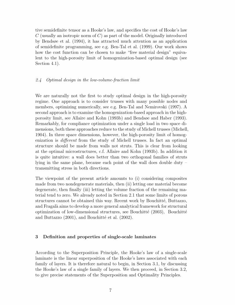
tive semidefinite tensor as a Hooke’s law, and specifies the cost of Hooke’s lawC (usually an isotropic norm of C) as part of the model. Originally introducedby Bendsøe et al. (1994), it has attracted much attention as an applicationof semidefinite programming, see e.g. Ben-Tal et al. (1999). Our work showshow the cost function can be chosen to make “free material design” equiva-lent to the high-porosity limit of homogenization-based optimal design (seeSection 4.1).
2.4 Optimal design in the low-volume-fraction limit
We are naturally not the first to study optimal design in the high-porosityregime. One approach is to consider trusses with many possible nodes andmembers, optimizing numerically, see e.g. Ben-Tal and Nemirovski (1997). Asecond approach is to examine the homogenization-based approach in the high-porosity limit, see Allaire and Kohn (1993b) and Bendsøe and Haber (1993).Remarkably, for compliance optimization under a single load in two space di-mensions, both these approaches reduce to the study of Michell trusses (Michell,1904). In three space dimensions, however, the high-porosity limit of homog-enization is different from the study of Michell trusses. In fact an optimalstructure should be made from walls not struts. This is clear from lookingat the optimal microstructures, c.f. Allaire and Kohn (1993b). In addition itis quite intuitive: a wall does better than two orthogonal families of strutslying in the same plane, because each point of the wall does double duty –transmitting stress in both directions.
The viewpoint of the present article amounts to (i) considering compositesmade from two nondegenerate materials, then (ii) letting one material becomedegenerate, then finally (iii) letting the volume fraction of the remaining ma-terial tend to zero. We already noted in Section 2.1 that some limits of porousstructures cannot be obtained this way. Recent work by Bouchitte, Buttazzo,and Fragala aims to develop a more general analytical framework for structuraloptimization of low-dimensional structures, see Bouchitte (2003), Bouchitteand Buttazzo (2001), and Bouchitte et al. (2002).
3 Definition and properties of single-scale laminates
According to the Superposition Principle, the Hooke’s law of a single-scalelaminate is the linear superposition of the Hooke’s laws associated with eachfamily of layers. It is therefore natural to begin, in Section 3.1, by discussingthe Hooke’s law of a single family of layers. We then proceed, in Section 3.2,to give precise statements of the Superposition and Optimality Principles.
7
3.1 The linear algebra of layering
Layered composites have been studied by many authors. The goal of thissubsection is to give a concise formula for the (degenerate) Hooke’s law C ofthe layered composite obtained by mixing volume fraction θ of Hooke’s law Awith volume fraction 1 − θ of void, in layers orthogonal to a fixed vector k.
If A is isotropic this is a very standard calculation. In terms of the Lamemoduli λ and µ, (i.e. if Aξ = 2µξ + λ(trξ)I), the composite’s Hooke’s law Csatisfies
〈Cξ, ξ〉 = θ
(〈Aξ, ξ〉 − 1
µ
|Aξk|2|k|2 +
λ + µ
µ(λ + 2µ)
〈Aξk, k〉2|k|4
). (1)
This is a special case of formula (5) below.
Remarkably, when A is anisotropic a simple formula is still possible. This mayat first seem an academic exercise, since for applications to optimal designit is natural to take A isotropic. But actually the extension is quite useful:permitting A to be an arbitrary Hooke’s law simplifies the notation. We shalluse the notation of Allaire (2002), adopting the projection-based viewpointof Allaire and Kohn (1993a). (Allaire’s book emphasizes the case when Ais isotropic, but one sees from the 1993 Allaire-Kohn paper that the caseof anisotropic A is no different.) The following calculation is, however, olderthan these references: it was first done for conductivity in Tartar (1985) andfor elasticity in Francfort and Murat (1986).
We begin with some notation: if MN is the space of all N × N symmetricmatrices and k is any nonzero vector, let W (k) be the subspace
W (k) = {η ∈ MN ; η · k = 0} (2)
(We think of this as the space of stresses compatible with layering direction k;here η · k is the product of the matrix η times the vector k.) The orthogonalcomplement of W (k) is
V (k) ={ξ ∈ MN ; ∃ a ∈ R
N such that ξ = a � k}
(3)
where a � k = 12(a ⊗ k + k ⊗ a).
For any (nondegenerate) Hooke’s law A, we have the orthogonal decomposition
MN = A1/2V (k) ⊕ A−1/2W (k). (4)
In other words, any ξ can be expressed uniquely as ξ = A1/2v + A−1/2wwith v ∈ V (k) and w ∈ W (k). We write ΠA1/2V (k)ξ and ΠA−1/2W (k)ξ for theorthogonal projections of ξ on these two subspaces.
8
We are ready to state the extension of (1) to anisotropic A: the Hooke’s law ofthe layered composite mixing A with void in layers normal to k is C = θf c
A(k)where θ is the volume fraction of A and
f cA(k) = A1/2ΠA−1/2W (k)A
1/2. (5)
In other words, the elastic energy quadratic form of the composite is
〈Cξ, ξ〉 = θ⟨A1/2ΠA−1/2W (k)A
1/2ξ, ξ⟩.
When A is isotropic, this reduces to (1). (An easy way to see this is to setAη = 2µη+λ(trη)I in equation (7) below, then do the indicated minimizationover v ∈ V (k).)
To explain the origin of (5), we start from fact that for the composite madeby layering two materials A and B in layers perpendicular to k with volumefractions θ and 1 − θ, the effective energy quadratic form is
minξ=θξA+(1−θ)ξB
ξB−ξA∈V (k)
θ〈AξA, ξA〉 + (1 − θ)〈BξB, ξB〉. (6)
The first constraint is equivalent to
ξA = ξ − (1 − θ)(ξB − ξA), ξB = ξ + θ(ξB − ξA),
and from the second constraint (1 − θ)(ξB − ξA) can be any element of V (k).Therefore (6) is equivalent to
minv∈V (k)
θ〈A(ξ + v), ξ + v〉 + (1 − θ)⟨B(ξ − θ
1−θv), ξ − θ
1−θv⟩.
When B = 0 we are left with
minv∈V (k)
θ〈A(ξ + v), ξ + v〉. (7)
The optimal v is such that A(ξ+v)⊥V (k), or equivalently A1/2(ξ+v)⊥A1/2V (k).Comparing this with the relation A1/2ξ = ΠA1/2V (k)A
We note for later use (in Section 5) that V (k), W (k), and f cA(k) depend only
on k/|k|, and that
f cA(k) = A − AfA(k)A. (8)
where
fA(k)ξ = A−1/2ΠA1/2V (k)A−1/2ξ. (9)
3.2 Single-scale laminates
A single-scale laminate is a high-porosity structure made from a fixed materialA. It consists of finitely many families of parallel beams in R
2, or finitely manyfamilies of parallel walls in R
3. The structure is determined by
(a) its rank: the number of families, an integer p ≥ 1;(b) its layer normals: unit vectors k1, . . . , kp, assumed distinct (i.e. ki 6= ±kj
for i 6= j);(c) its layer proportions: positive real numbers t1, . . . , tp with
∑pi=1 ti = 1.
We are interested in the high-porosity limit, so there is also a scale factor θ,representing (to leading order) the volume fraction of material. The physicalstructure of interest consists of layers of thickness θti normal to ki, 1 ≤ i ≤ p.
The actual geometry of the composite is not fully determined by these param-eters. For example, a triangular lattice and a Kagome lattice have the samelayer normals and proportions (see Figure 1). We shall prove, however, that toleading order as θ → 0, the Hooke’s law of such a composite depends only onthe layering normals and proportions. Therefore it is not useful to distinguishbetween different structures with the same layer normals and proportions.
The base material A can be isotropic or anisotropic. In the anisotropic case,however, we assume its orientation is fixed. (Thus the orientation is not per-mitted to depend on the layer normal.)
Our focus is on the linearly elastic behavior of this porous composite. If thelayering directions are rationally related then the structure is spatially peri-odic, with a (possibly large) period cell. The general case can be approximatedby such structures, so periodic homogenization is sufficient for proving theo-rems about the effective behavior. In this setting the local Hooke’s law is Awhere there is material and 0 where there isn’t; in other words it equals χ(y)Awhere χ is a periodic function taking only values 0 and 1. Evidently
χ =p∑
i=1
χi − g(ov), (10)
10
where χi is the characteristic function of the ith family of layers (a periodicfunction of y · ki, taking only the values 0 and 1, with average value θti) andg(ov) is supported in the region where the layers overlap. The overlap termis bounded by the number of families (0 ≤ g(ov) ≤ p) and the volume of itssupport is of order θ2, so ∫
Y|g(ov)(x)| dx = O(θ2).
Our focus is on the leading-order behavior as θ → 0; therefore quantities oforder θ2 will always be treated as error terms.
Having defined the notion of a single-scale laminate, we now give careful state-ments of the Superposition and Optimality Principles:
(1) Superposition Principle: Let C(s)p be the effective Hooke’s law of a
rank–p single-scale laminate with normals {ki}pi=1, proportions {ti}p
i=1,and scale factor θ. Then
C(s)p = θ
p∑i=1
tifcA(ki) + O(θ2). (11)
(2) Optimality Principle: Let C be the effective Hooke’s law of a high-porosity composite made by mixing a fixed material A with void, involume fractions θ and 1− θ respectively. Then there exists a single-scalelaminate C
(s)+ with same volume fraction that is at least as stiff in the
sense thatC ≤ C
(s)+ + O(θ2). (12)
The proofs will be given in Section 5, but let us make a few comments here.Concerning the Superposition Principle: if the different families of layers didnot intersect then superposition would be obvious. But they do intersect, andthis appears to impose a kinematic constraint linking the elastic deformationsof the distinct families of layers. In proving the Superposition Principle, wewill effectively be showing that this constraint is not important in the highporosity limit. Concerning the Optimality Principle: an analogous statementis known for sequential laminates. Therefore the principle can be proved byeither (a) comparing the Hooke’s law of a single-scale laminate with that ofthe associated sequential laminate – showing that the two agree to leadingorder in θ; or (b) repeating the arguments used for sequential laminates in thecontext of single-scale laminates. The latter approach turns out to be easier,but we also discuss the former since the connection between sequential andsingle-scale laminates is of independent interest.
It is natural to wonder whether the layers might buckle. The analysis of buck-ling in elastic composites is complicated, because buckling can be initiated atany length scale (microscopic, macroscopic, or in between). We do not attempt
11
to address it here, except to note that buckling seems unlikely if the stressesin the layers are tensile. Our analysis in Section 5 gives more than the justthe Hooke’s law of the composite – it also identifies the stress in each layer.Thus it gives sufficient information to check a criterion for microbuckling.
Our attention is on the high-porosity limit, so we often ignore terms of order θ2
and drop the scale factor θ. Thus, in Section 4 where we focus on the optimalselection of single-scale laminates, we take the view that the Hooke’s law of asingle-scale laminate is
p∑i=1
tifcA(ki). (13)
Notice that the set of possible Hooke’s laws (13) is precisely the convex hullof {f c
A(k)} as k ranges over the unit sphere.
Because (13) is linear, there are in general many single-scale laminates witha given Hooke’s law. For example, if A is isotropic and we work in 2D, anyrotation of a triangular lattice gives the same isotropic Hooke’s law. Moreoverif two single-scale laminates give the same Hooke’s law
p∑i=1
tifcA(ki) =
q∑j=1
sjfcA(nj)
then so does any affine combination (using proportions αti for layer normals{ki} and proportions (1 − α)sj for layer normals {nj}, 0 < α < 1). By asuitable limiting procedure, one can also consider structures with a continuumof layering directions. Returning to our previous example, if A is isotropic in2D, then besides rotated triangular lattices, we also get an isotropic Hooke’slaw by taking the layer directions to be uniformly distributed on the unitcircle.
4 Numerical applications
Many pages have been devoted to bounds on the effective moduli of com-posites. These bounds determine, at least implicitly, the minimum density aporous composite must have to achieve a specified stiffness. But extracting thisinformation numerically is not an easy matter. Moreover though the theorysupplies microstructures achieving the bounds, they are typically sequentiallaminates, which are difficult or impossible to manufacture due to the require-ment of multiple length scales. When the theory offers us simpler structures(e.g. Hashin’s concentric sphere construction, or the Vigdergauz microstruc-ture) there is no systematic method for classifying or choosing between them.Numerical structural optimization has been used to find extremal microstruc-tures, for example by Sigmund (1994), but again the task is difficult and its
12
solution is unsystematic.
Optimal design in the high-porosity regime is, by contrast, dramatically sim-pler. This is because the only composites we need to consider are single-scalelaminates (for applications where stiffness is preferred).
This section demonstrates the extent of the simplification by discussing threesimple but practical problems:
(a) finding the minimum density required for a given stiffness, as an applica-tion of semidefinite programming (Section 4.1);
(b) finding the “simplest” single-scale laminate with a given Hooke’s law, asan application of linear programming (Section 4.2); and
(c) finding a continuously-varying family of single-scale laminates that achievea continuously-varying family of Hooke’s laws, as an application of quadraticprogramming (Section 4.3).
We elaborate briefly on (b) and (c). It is no surprise that many differentstructures have the same Hooke’s law. This is clear from counting parameters(the class of all structures has many more degrees of freedom than the class ofall Hooke’s laws). The resulting redundancy is a gift from nature: it permits usto optimize the elastic response (which involves only the Hooke’s law) and alsosomething else. There are many reasonable choices for the secondary criterion.We focus in (b) and (c) on “simplicity” and “continuity,” since these propertiesare clearly desirable for manufacturability.
4.1 Minimizing density
We address the following problem: given a Hooke’s law C0, find a microstruc-ture S and its associated Hooke’s law CS solving
min {density(S) ; CS ≥ C0 , CS achieved by the microstructure S} . (14)
In the high-porosity regime, it suffices by the Optimality Principle to considermicrostructures in the class of single-scale laminates. Therefore (14) reducesto the optimization
minτ1,...,τp≥0
k1,...,kp∈SN−1∑p
i=1τifc
A(ki)≥C0
p∑i=1
τi. (15)
Here N = 2 for 2D structures and N = 3 for 3D structures (SN−1 is theunit circle in R
2 when N = 2 and the unit sphere in R3 when N = 3). The
constraint∑p
i=1 τifcA(ki) ≥ C0 means that the associated quadratic forms are
13
well-ordered: ⟨ p∑i=1
τifcA(ki)ξ, ξ
⟩≥ 〈C0ξ, ξ〉 (16)
for any N × N symmetric matrix ξ. The parameters {τi} represent {θti};thus the single-scale laminate has density θ =
∑τi and layering proportions
ti = τi/θ.
The rank of the single-scale laminate (the value of p) seems at first to be partof the optimization. However it is easy to see that p need not be large, sinceeach point in the convex hull of {f c
A(k)}k∈SN−1 is a convex combination of atmost d + 1 extreme points, where d = d(N) is the dimension of the space ofHooke’s laws. (If A is isotropic – the case of primary physical interest – onecan do better: using the special form of f c
A(k) in that case, Francfort et al.(1995) have shown that it suffices to consider p = 3 in two space dimensionsand p = 6 in 3D.)
We want to solve (15) numerically. One could imagine taking the theoreticalminimum value of p and optimizing over the τ1, . . . τp and k1, . . . , kp. This isnot very convenient, however, since the stiffness constraint is nonlinear in ki.
Our approach is different. Since ki can be any unit vector and p can be large,we view the expression
∑pi=1 τif
cA(ki) as a discretized integral over the unit
sphere of a function τ(k)f cA(k). Discretizing systematically, we let k range
over a large but fixed set of M unit vectors k1, . . . , kM (equispaced on theunit circle in R
2, or approximately equispaced on the unit sphere in R3). Our
numerical problem is thus
minτ1,...,τM≥0∑M
i=1τif
cA(ki)≥C0
M∑i=1
τi. (17)
Since the layering directions have been fixed, the optimization is only overτ1, . . . , τM .
The positivity constraint (16) is linear with respect to τi, so (17) has the formof a semi-definite program (see for example Vandenberghe and Boyd (1996)).Efficient algorithms and software have been developed for such problems inrecent years using interior-point methods. The semidefinite programs solvedin this paper were all done using the SP software package, originally developedby Vandenberghe and Boyd.
Figure 2(a) shows the solution of (17) obtained by semidefinite programming intwo space dimensions with C0 is isotropic. The half-unit circle was discretizedby M = 100 equispaced orientations. Each line in the figure has normal ki andthickness τi.
14
We observed in Section 3.2 that there are many different single-scale lami-nates with the same isotropic Hooke’s law and the same (minimal) weight.As the figure shows, our semidefinite programming approach selects the onethat uses all the available layering directions with equal weights. This is notsurprising, given the symmetry of the problem and the interior-point charac-ter of the algorithm. Additional examples of semidefinite programming (withC0 orthotropic) will be discussed in Section 4.3 (see Figures 3(a)-(c)). Thoseexamples confirm that our approach via semidefinite programming usuallyproduces relatively uniform structures, using many if not all the availablelayering directions.
4.2 Maximizing simplicity
Since many single-scale laminates have the same Hooke’s law, it is naturalto select a particular solution by optimizing something else. If the goal ismanufacturability, it seems natural to look for a structure with relatively fewlayering directions.
This goal can be achieved by conventional linear programming. Continuing ourfocus on minimal density, suppose C1 is the Hooke’s law of an optimal single-scale laminate (obtained by semidefinite programming as explained above)and θ =
∑Mi=1 τi is its density. We seek another single-scale laminate with
the same Hooke’s law and density but just a few active layers. To find it, wemaximize the thickness in a particular direction. Specifically, if the initially-given single-scale laminate has maximal thickness in layering direction kl, wesolve
maxτ1,...,τM≥0∑M
i=1τi=θ∑M
i=1τifc
A(ki)=C1
τl. (18)
Since the stiffness constraint is now linear, this is a linear program. It canbe solved by the the simplex method. Since simplex method always returns avertex of the feasible set, the solution will have most of its layering parametersτi equal to zero – indeed (barring degeneracy) it will minimize the numberof active directions. This is what is observed numerically. For example, whenC1 is isotropic the resulting single-scale composite uses just three equispacedlayering directions, corresponding to a triangular or Kagome lattice (see Figure2(b)).
15
(a) Result of the semidef-inite program discussed inSection 4.1.
(b) Simplification via lin-ear programming, as dis-cussed in Section 4.2.
Fig. 2. Minimum-density single-scale laminates in two space dimensions, i.e. solu-tions of (14). The Hooke’s law C0 was chosen to be isotropic with Lame moduliλ = 1 and µ = 0.5. The underlying elastic material was also chosen isotropic,also with Lame moduli λ = 1 and µ = 0.5. The half-unit-circle was discretized byM = 100 equispaced directions. Each figure shows the layer thicknesses of the asso-ciated single-scale laminate by superimposing segments of thickness τi and normalki.
4.3 Enforcing continuity
The preceding examples address the optimal design of macroscopically uniformmicrostructures. We turn now to a different type of problem: the optimaldesign of a macroscopically heterogeneous structure.
The starting point we have in mind is the output of a homogenization-basedor free-material-design-based design algorithm. It would specify the desiredHooke’s law and density as a function of position in the design domain. To passfrom this information to an actual design, one must “fill in the microstructure”by specifying, for each point in the design domain, a microstructure withthe proposed Hooke’s law and density. These structures can then be piecedtogether. Thinking numerically: if the macroscopic Hooke’s law is piecewiseconstant on a triangulation of the design domain, then each triangle would befilled with a uniform microstructure achieving the desired properties.
If the macroscopic structure varies smoothly, it is natural to ask that themicrostructure also vary smoothly. We shall explain how this can be achievedwithin the class of single-scale laminates by solving a quadratic program.
To capture the main idea in the simplest possible setting, we suppose themacroscopic Hooke’s law C and density θ depend only on one coordinate x1,taking values {Cj}K
j=1 and {θj}Kj=1 at evenly-spaced nodes along the x1 axis.
We also suppose these Hooke’s laws and densities are achievable by single-scale laminates. (If not, we would solve (14) – or more precisely (17) – at each
16
node, to replace Cj with a Hooke’s law that is at least as stiff, at least as light,and achievable by a single-scale laminate.)
Our strategy is simple. We work, as in Sections 4.1 and 4.2, with single-scale laminates using a fixed collection of layer normals {ki}M
i=1. The single-scale laminate at node j is described by its vector of layer thicknesses τ j =(τ j
1 , . . . τ jM). To achieve continuous dependence, we will minimize the “Dirichlet
norm” of the spatial variation
K∑j=1
∑i neighbor of j
d2(τ i, τ j
) (19)
where d(τ, τ ′) measures the “distance” between the single-scale laminates as-sociated with τ and τ ′. The optimization is over the layering parameters at allnodes, τ j
k ≥ 0, 1 ≤ j ≤ K, 1 ≤ k ≤ M , subject to constraints on the densityand Hooke’s law at each node:
M∑i=1
τ ji = θj , 1 ≤ j ≤ K, (20)
andM∑i=1
τ ji f c
A(ki) = Cj , 1 ≤ j ≤ K. (21)
We come now to the main issue: the choice of the “distance” d. It seems naturalto ask that
(i) d2 be quadratic in the layering parameters, and(ii) if two single-scale laminates differ only by a spatial rotation, their “dis-
tance” be proportional to the angle of the rotation.
The first property is desirable because it makes the minimization of (19) aquadratic optimization. The second reflects our viewpoint that a small rotationis a minor change of the structure, though it may involves dramatic changesin the individual layer thicknesses.
Condition (ii) is very restrictive. For example the l2 distance
‖τ − τ ′‖l2 =
[M∑i=1
(τi − τ ′i)
2
]1/2
does not have this property. In fact, working in two space dimensions withan even number of layering directions {ki} equispaced on the unit half-circle,consider the choice τi = c if i is even and τi = 0 if i is odd. If τ ′
i+1 = τi thenτ ′ corresponds to a rotation of τ by a small angle, but the distance betweenthem is huge. Thus the l2 distance is not an appropriate choice for d.
17
In fact, condition (ii) is too restrictive. There seems to be no distance d sat-isfying both (i) and (ii). However we obtained good numerical results using
d(τ, τ ′) = ‖F ∗ (τ − τ ′)‖l2, (22)
where F∗ denotes a discrete convolution filter given by
(F ∗ τ)i =1
2r + 1
r∑j=−r
τi+j , (23)
and r is a fixed parameter (the bandwidth of the filter). Here we use theconvention that the indices of τ are extended cyclically (τ0 = τM , τM+1 =τ1, etc). The parameter r must be reasonably large, to avoid the difficultiesassociated with the l2 norm; however 2r + 1 must be below M , since when2r + 1 = M the convolution F ∗ τ sees only the volume fraction
∑τi.
Figure 3 shows the performance of this scheme. Working in two space dimen-sions, we used M = 51 layering directions, equispaced on the unit half-circle.For the initial (continuously-varying) Hooke’s law we took C to be a functionof x1 ∈ [0, 1], interpolating linearly between
• at x1 = 0: the isotropic law with Lame moduli λ = .4166 and µ = 0.4166(corresponding to Young’s modulus E = 2 and Poisson’s ratio ν = .2 inplane stress), and
• at x1 = 1: the orthotropic law associated with a two-layer single-scale lam-inate, using τ1 = 2 when the layer normal has angle π/2 and τ2 = .5 whenthe layer normal has angle 0.
The underlying material A was also chosen isotropic, with Lame moduli λ =.476 and ν = .357 (corresponding to Young’s modulus E = 1 and Poisson’sratio ν = .4 in plane stress).
We discretized the interval 0 ≤ x1 ≤ 1 using 10 equispaced nodes. Since theisotropic and orthotropic laws are both associated with single-scale laminates,preprocessing by the method of Section 4.1 is not necessary. But it is interest-ing to see what such preprocessing gives, since it reveals the character of theselections made by our semidefinite program (17). The results are shown in thetop row of Figure 3. The dependence is continuous in x1, but the semidefiniteprogram uses many layering directions (favoring uniformity).
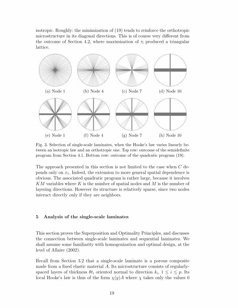
The bottom row of Figure 3 shows the result of minimizing (19) subject to (20)and (21), when the distance d is given by (22)-(23) with r = 15. (Recall thatM = 51, so (2r + 1)/M ≈ 3/5.) The resulting structures depending continu-ously on x1, and they also use relatively few layers. Interestingly, the layers inthe rightmost figure are active (even dominant) in all simplified microstruc-tures. This is true even at x1 = 0 (Figure 3(e)), where the Hooke’s law is
18
isotropic. Roughly: the minimization of (19) tends to reinforce the orthotropicmicrostructure in its diagonal directions. This is of course very different fromthe outcome of Section 4.2, where maximization of τl produced a triangularlattice.
(a) Node 1 (b) Node 4 (c) Node 7 (d) Node 10
(e) Node 1 (f) Node 4 (g) Node 7 (h) Node 10
Fig. 3. Selection of single-scale laminates, when the Hooke’s law varies linearly be-tween an isotropic law and an orthotropic one. Top row: outcome of the semidefiniteprogram from Section 4.1. Bottom row: outcome of the quadratic program (19).
The approach presented in this section is not limited to the case when C de-pends only on x1. Indeed, the extension to more general spatial dependence isobvious. The associated quadratic program is rather large, because it involvesKM variables where K is the number of spatial nodes and M is the number oflayering directions. However its structure is relatively sparse, since two nodesinteract directly only if they are neighbors.
5 Analysis of the single-scale laminates
This section proves the Superposition and Optimality Principles, and discussesthe connection between single-scale laminates and sequential laminates. Weshall assume some familiarity with homogenization and optimal design, at thelevel of Allaire (2002).
Recall from Section 3.2 that a single-scale laminate is a porous compositemade from a fixed elastic material A. Its microstructure consists of regularly-spaced layers of thickness θti oriented normal to direction ki, 1 ≤ i ≤ p. Itslocal Hooke’s law is thus of the form χ(y)A where χ takes only the values 0
19
and 1, and
χ =
( p∑i=1
χi
)− g(ov), (24)
where χi is the characteristic function of the ith family of layers (a periodicfunction of y · ki, taking only the values 0 and 1, with average value θti) andg(ov) is supported in the region where the layers overlap (with 0 ≤ g(ov) ≤ p).
If the layering directions are rational then the structure is periodic, with a(possibly large) period cell. The general case can be approximated by suchstructures, so periodic homogenization is sufficient for proving theorems aboutthe effective behavior. Morover, since homogenization is a scale-invariant the-ory, there is no loss of generality in rescaling the structure so the unit cell isY = [0, 1]N . We shall work throughout this section in these rescaled variables.
In discussing the Hooke’s law of a single-scale laminate, our starting point isthe familiar variational principle
⟨C(s)
p ξ, ξ⟩
= infΦ∈H1
#
∫〈χ(y)A(ξ + e(Φ)), ξ + e(Φ)〉 dy (25)
where the integral is over the period cell Y = [0, 1]N and χ has the form(24). Here and throughout this section, H1
# denotes the class of Y -periodicH1 functions.
5.1 The Superposition Principle
We shall prove upper and lower bounds that agree to leading order in volumefraction.
5.1.1 The lower bound
The primal variational principle (25) characterizes⟨C(s)
p ξ, ξ⟩
by a minimiza-tion over kinematically admissible periodic strain fields. For the lower bound,however, it is more convenient to work with its convex dual – a maximizationover statically admissible periodic stress fields. We briefly review its well-known derivation, as an application of convex duality. Starting from (25) wehave ⟨
C(s)p ξ, ξ
⟩= inf
Φ∈H1#
supσ(y)
∫2〈σ, ξ + e(Φ)〉 −
⟨(χ(y)A)−1σ, σ
⟩dy
20
where σ ranges over periodic “stress fields” that vanish where χ = 0. A stan-dard duality theorem permits us to interchange the inf and sup, leading to
⟨C(s)
p ξ, ξ⟩
= supσ
infΦ∈H1
#
∫2〈σ, ξ + e(Φ)〉 −
⟨(χ(y)A)−1σ, σ
⟩dy
= supdivσ=0
2〈σ, ξ〉 − −∫
Y
⟨(χ(y)A)−1σ, σ
⟩dy.
where σ denotes the average of σ. Recall that to be admissible for this dualvariational principle, σ should be a periodic, symmetric-matrix-valued func-tion that vanishes on the “holes” (where χ = 0). The constraint divσ = 0 is ofcourse understood in the “weak sense:” σ must be divergence-free where thereis material, and its normal traction σ · n must vanish at the boundaries of allholes.
We apply this with a “stress field” of the form
σ =p∑
i=1
χi(y)σi,
where χi is the characteristic function of the layers with normal ki and σi
is a (constant) element of W (ki). This choice is admissible, because eachterm χi(y)σi is admissible. To see why, we note (fixing i) that the conditionσi ∈ W (ki) is equivalent to σi · ki = 0. Thus the piecewise-constant test fieldχi(y)σi is periodic and weakly divergence free, and it vanishes where there isno material. Our stress field σ has mean
σ = θp∑
i=1
tiσi + O(θ2)
since the region where the layers overlap has volume fraction of order θ2. Weconclude from the dual variational principle that
⟨C(s)
p ξ, ξ⟩≥ 2θ
p∑i=1
ti〈σi, ξ〉 − θp∑
i=1
ti⟨A−1σi, σi
⟩+ O(θ2). (26)
for any choice of σi ∈ W (ki).
We now choose the σi to maximize the order-θ terms on the right hand sideof (26). The optimality condition says that for each i, 2θtiξ − 2θtiA
−1σi isorthogonal to W (ki). Since 2θti 6= 0, we conclude that {σi}p
i=1 are optimalprecisely when
ξ − A−1σi ∈ V (ki) for each i. (27)
In fact, the optimal σi can be given explicitly:
σi = A1/2ΠA−1/2W (ki)A1/2ξ = f c
A(ki)ξ, (28)
21
using the notation introduced in Section 3.1. To justify (28), we need only showthat this choice of σi satisfies (27). Recall from (4) that the space of N × Nsymmetric tensors has the orthogonal decomposition A1/2V (ki)⊕A−1/2W (ki).So A1/2ξ can be written uniquely as
A1/2ξ = A1/2ηi + A−1/2σi
with ηi ∈ V (ki) and σi ∈ W (ki). Clearly these σi satisfy (27). Since A−1/2σi =ΠA−1/2W (ki)A
1/2ξ by definition, we have demonstrated (28).
Finally we evaluate the lower bound (26) at the optimal σi. Taking the innerproduct of (27) with σi gives
⟨A−1σi, σi
⟩= 〈σi, ξ〉.
Therefore the order-θ terms on the right side of (26) reduce to θ∑p
i=1 ti〈σi, ξ〉.Replacing σi by its characterization (28), we conclude that
⟨C(s)
p ξ, ξ⟩≥ θ
p∑i=1
ti〈f cA(ki)ξ, ξ〉 + O(θ2),
or in other words
C(s)p ≥ θ
p∑i=1
tifcA(ki) + O(θ2). (29)
This is the desired lower bound.
5.1.2 The upper bound
Our proof of the matching upper bound uses the Hashin-Shtrikman variationalprinciple. To make the discussion self-contained, we start by reviewing itsderivation. Starting from (25), we add and subtract the “reference energy”〈A(ξ + e(Φ)), ξ + e(Φ)〉 to get
Substituting this into (30), we conclude that for any η ∈ MN ,
⟨C(s)
p ξ, ξ⟩≤ inf
Φ∈H1#
∫Y〈A(ξ + e(Φ)), ξ + e(Φ)〉 dy
−∫
2(1 − χ(y))〈η, ξ + e(Φ)〉 − (1 − χ(y))⟨A−1η, η
⟩dy.
Integrating all terms that don’t involve e(Φ), writing
Θ =∫
χ(y) dy = θ + O(θ2) (31)
for the exact volume fraction of the composite, and using the fact that e(Φ)has mean value 0, we conclude that⟨
C(s)p ξ, ξ
⟩≤ 〈Aξ, ξ〉 + (1 − Θ)
⟨A−1η, η
⟩− 2(1 − Θ)〈η, ξ〉 + I(η), (32)
where
I(η) = infΦ∈H1
#
∫〈A e(Φ), e(Φ)〉 + 2χ(y)〈η, e(Φ)〉 dy. (33)
We can express I(η) in terms of the Fourier transform of χ as follows. ByParseval’s theorem,
I(η) = infΦ∈H1
#
∑k∈ZN\{0}
⟨Ae(Φ)(k), e(Φ)(k)
⟩+ 2χ(k)
⟨η, e(Φ)(k)
⟩.
Now, Φ ∈ H1#(Y ) is equivalent to e(Φ)(k) ∈ V (k) for each k ∈ Z
N \ {0} and
e(Φ)(0) = 0. (To keep the notation simple, we do not distinguish between V (k)and its complexification.) The minimization over Φ can be done separately at
each frequency: introducing the notation ek := e(Φ)(k), we have
I(η) =∑
k∈ZN\{0}inf
ek∈V (k)〈Aek, ek〉 + 2χ(k)〈η, ek〉
=∑
k∈ZN\{0}inf
ek∈V (k)
⟨A1/2ek, A
1/2ek
⟩+ 2χ(k)
⟨A−1/2η, A1/2ek
⟩=
∑k∈ZN\{0}
infϕk∈V (k)
{∣∣∣A1/2ek + χ(k)A−1/2η∣∣∣2 − |χ(k)|2
∣∣∣A−1/2η∣∣∣2} .
The optimal choice of ek is now clear: it is
ek = −A−1/2ΠA1/2V (k)χ(k)A−1/2η,
and substitution gives the value of I(η):
I(η) =∑
k∈ZN\{0}|χ(k)|2
(∣∣∣ΠA−1/2W (k)A−1/2η
∣∣∣2 − ∣∣∣A−1/2η∣∣∣2) .
23
This can be expressed more compactly using the notation introduced in Sec-tion 3.1:
I(η) = − ∑k∈ZN\{0}
|χ(k)|2 〈fA(k)η, η〉,
with fA(k)ξ = A−1/2ΠA1/2V (k)A−1/2ξ. Thus the Hashin-Shtrikman bound (32)
says⟨C(s)
p ξ, ξ⟩≤ 〈Aξ, ξ〉+(1−Θ)
⟨A−1η, η
⟩−2(1−Θ)〈η, ξ〉− ∑
k∈ZN\{0}|χ(k)|2 〈fA(k)η, η〉.
for any η ∈ MN . We could optimize over η, but it isn’t necessary. Rather, wesimply take η = Aξ. This gives⟨
C(s)p ξ, ξ
⟩≤ Θ〈Aξ, ξ〉 − ∑
k∈ZN\{0}|χ(k)|2 〈fA(k)Aξ, Aξ〉. (34)
We have not yet used the hypothesis that the microstructure is a single-scalelaminate: (34) applies to any porous composite made from the basic materialA.
For a single-scale laminate we can go further: we shall show that
∑k∈ZN\{0}
|χ(k)|2 〈fA(k)Aξ, Aξ〉 = θp∑
i=1
ti〈fA(ki)Aξ, Aξ〉 + O(θ2). (35)
Indeed, by (24) the left hand side of (35) is equal to
∑k∈ZN\{0}
∣∣∣∣∣p∑
i=1
χi(k) − g(ov)(k)
∣∣∣∣∣2
〈fA(k)Aξ, Aξ〉. (36)
Since χi(y) is a function of ki · y, its Fourier transform χi(k) vanishes unlessk ‖ ki. Since the layering directions {ki} are assumed to be distinct, it followsthat for i 6= j we have
χi(k)χj(k) = 0 for all k.
Therefore (36) equals
∑k∈ZN\{0}
[ p∑i=1
(|χi(k)|2 − 2χi(k) · g(ov)(k)
)+∣∣∣g(ov)(k)
∣∣∣2] 〈fA(k)Aξ, Aξ〉.
The terms involving g(ov) are of order O(θ2). To see this, observe using (9)that
|〈fA(k)Aξ, Aξ〉| =∣∣∣⟨ΠA1/2V (k)A
1/2ξ, A1/2ξ⟩∣∣∣ ≤ ‖A1/2ξ‖2;
24
in particular it is uniformly bounded, independent of k. Since the support ofg(ov) has volume of order θ2 and g(ov) is pointwise less than or equal to p, anapplication of Plancherel’s theorem gives
∑k∈ZN\{0}
∣∣∣g(ov)(k)∣∣∣2 = O(θ2).
Similarly,
∑k∈ZN\{0}
χi(k) · g(ov)(k) =∑
k∈ZN
χi(k) · g(ov)(k) − χi(0)g(ov)(0)
=∫
χi(y)g(ov)(y) dy −O(θ3) = O(θ2),
since χi(y)g(ov)(y) ≤ g(ov)(y) and∫
g(ov)(y) dy = O(θ2). Thus (36) equals
∑k∈ZN\{0}
p∑i=1
|χi(k)|2 〈fA(k)Aξ, Aξ〉 + O(θ2) (37)
as asserted.
To evaluate (37), we recall that for each i, χi(y) is a periodic function ofy taking only values 0 and 1, with average value χi = tiθ. Therefore, byPlancherel’s theorem,∑
k∈ZN\{0}|χi(k)|2 =
∫|χi − χi|2 dy = tiθ(1 − tiθ).
Substituting this into (37) and summing over i, we obtain the desired formula(35) for the nonlocal term in the Hashin-Shtrikman bound.
Wrapping up: when the microstructure is a single-rank laminate, the totalvolume fraction is Θ = θ
∑pi=1 ti +O(θ2) and the upper bound (34) reduces to
via (35) to
⟨C(s)
p ξ, ξ⟩≤ θ
p∑i=1
ti [〈Aξ, ξ〉 − 〈fA(ki)Aξ, Aξ〉] + O(θ2).
Recalling from (8) that A − AfA(k)A = f cA(k), we have shown that
C(s)p ≤ θ
p∑i=1
tifcA(ki) + O(θ2), (38)
in the sense of quadratic forms. This is the desired upper bound. Taken to-gether, (29) and (38) prove the validity of the Superposition Principle.
Remark 5.1 Stresses in the layers. Since the lower and upper boundsmatch at leading order, each of the inequalities that led to the bounds must
25
actually be an equality at leading order. In particular, our lower bound (26)becomes
⟨C(s)
p ξ, ξ⟩
= 2θp∑
i=1
ti〈σi, ξ〉 − θp∑
i=1
ti⟨A−1σi, σi
⟩+ O(θ2)
when
σi = A1/2ΠA−1/2W (ki)A1/2ξ.
It follows that σi is (to leading order) the stress in the ith family of layers.
Remark 5.2 Comparing the proofs of the lower and upper bounds.We proved the lower bound in Section 5.1.1 by applying the dual variationalprinciple to a superposition of admissible piecewise-constant “stress fields”χi(y)σi. The argument worked because the supports of these “stress fields”were almost disjoint: σ =
∑i χi(y)σi vanishes where there is no material and
equals σi in the ith family of layers, except in the regions where layers overlap(whose volume is O(θ2)). It is natural to ask whether the upper bound canbe proved by a similar argument. The answer, we think, is no. The reason isthat the analogous piecewise-constant “strain fields” for a layered compositedo not vanish in the void. It is of course possible to consider a superposition of(kinematically admissible) piecewise-constant strain fields associated with thedifferent layering directions; however they would interact, making an argumentparallel to Section 5.1.1 impossible.
5.2 Proof of the Optimality Principle
The Optimality Principle is the analogue for single-scale laminates of a well-known result from Avellaneda (1987). That work considered two-componentcomposites made from two well-ordered, nondegenerate materials with Hooke’slaws B < A. It showed the “optimality” of sequential laminates (for problemswhere stiffness is preferred), by proving that if C is the Hooke’s law of anycomposite then there is a sequential laminate – made from the same twomaterials, using the same volume fractions – whose Hooke’s law C
(l)+ satisfies
C ≤ C(l)+ . The proof had two main ingredients: the Hashin-Shtrikman upper
bound, and an exact formula for the Hooke’s law of a sequential laminate.
Our Optimality Principle follows (at least formally) from Avellaneda’s result,by (i) passing to the limit B → 0, then (ii) using the results in Section 5.3,which relate the Hooke’s laws of single-scale and sequential laminates. Butit is simpler and much more direct to give a self-contained proof, applyingthe strategy of Avellaneda’s argument directly to the setting of single-scalelaminates. Since the main ingredients – the Hashin-Shtrikman bound and aformula for the Hooke’s law – are already in hand, the proof is quite short.
26
We start from the Hashin-Shtrikman upper bound (34), which can be writtenas
C ≤ ΘA − ∑k∈ZN\{0}
|χ(k)|2 AfA(k)A. (39)
Recall that we proved this for any porous composite, not just single-ranklaminates. The function χ was the characteristic function of the microstructure(in other words, the local Hooke’s law was χ(y)A) and Θ was the volumefraction where χ = 1. By Plancherel,
∑k∈ZN\{0}
|χ(k)|2 =∫
|χ − Θ|2 dy = Θ(1 − Θ);
and by (8) we have A − AfA(k)A = f cA(k), so (39) can be written
C ≤ Θ∑
k∈ZN\{0}tkf
cA(k) + O(Θ2)
with tk = |χ(k)|2 /Θ(1− Θ). Since∑
tk = 1, the sum on the right is a convexcombination of the degenerate Hooke’s laws {f c
A(k)}. In other words, it liesin the closed convex hull of {f c
A(k)}k∈SN−1 (recall that f cA(k) depends only
on k/|k|). By Caratheodory’s theorem, every point in this set is a convexcombination of finitely many extreme points. Therefore there exist positivenumbers t′1, . . . , t
′p (with
∑t′i = 1) and unit vectors k′
1, . . . k′p such that
∑k∈ZN\{0}
tkfcA(k) =
p∑i=1
t′ifcA(k′
i), (40)
whence
C ≤ Θp∑
i=1
t′ifcA(k′
i) + O(Θ2).
This proves the Optimality Principle (12): C is, to leading order, less than orequal to the Hooke’s law
C(s)+ = Θ
p∑i=1
t′ifcA(k′
i)
of a single-scale laminate made from the same material A using the samevolume fraction Θ.
Remark 5.3 What if compliance is preferred? The Optimality Princi-ple says that for any porous composite C, there is single-scale laminate withthe same volume fraction that’s stiffer (to leading order) than C. Is there alsoa single-scale laminate that’s more compliant? We think not. (For example,if the base material A is isotropic then there is only one isotropic compositeC that’s achievable as a single-scale laminate; it is, by the Optimality Prin-ciple, the stiffest isotropic high-porosity composite achievable by mixing A
27
with void.) However if C is nondegenerate (that is, if C > 0), then there areplenty of single-scale composites with the same volume fraction that are morecompliant. To achieve this, let θ be the volume fraction of material in C, andconsider any single-scale laminate with the same volume fraction; suppose itsHooke’s law is Cssl = θ
∑i tif
cA(ki). If C is nondegenerate then we can choose
α > 0 small enough that αCssl ≤ C. Thus there is a single-scale laminatewith volume fraction αθ that’s more compliant than C. Now, for porous com-posites it is always easy to “waste” material – it suffices to include, as partof the unit cell, a region of material that’s disconnected from the rest of thestructure. By starting from the single-scale laminate with volume fraction αθthen “wasting” volume fraction (1 − αθ), we obtain a porous composite withvolume fraction θ that’s more compliant than C. It is not a single-scale lami-nate, but it is certainly a porous composite with a relatively simple single-scalemicrostructure.
5.3 Single-scale and sequential laminates
The optimal design literature has devoted a lot of attention to sequentiallaminates, because for problems where stiffness is preferred an optimal mi-crostructure can always be found in this class.
Our single-scale laminates can be viewed as “sequential laminates without theseparation of scales.” Indeed, the optimal two-component sequential laminatesconsidered in the optimal design literature mix two well-ordered materialswith Hooke’s laws B < A. We shall show that when B = 0, the Hooke’slaw of a sequential laminate agrees to leading order with the Hooke’s law ofthe associated single-scale laminate. Thus the separation of scales implicit insequential lamination is unimportant in the high-porosity limit.
A single-scale laminate has layers of thickness θti oriented normal to ki, 1 ≤i ≤ p. Here θ is a scale factor (the volume fraction, to leading order) and therelative thicknesses are normalized by
∑pi=1 ti = 1. We define a corresponding
sequential laminate with Hooke’s law C(l)p by the following iterative procedure:
Fixing two Hooke’s laws B < A,
• let C(l)1 be the Hooke’s law of the composite obtained by mixing A and B
in layers normal to k1, using volume fraction θt1 of A;• then for 2 ≤ i ≤ p, let C
(l)i be the Hooke’s law of the composite obtained
by mixing A with C(l)i−1 in layers normal to ki, using volume fraction θti of
A and (1 − θti) of C(l)i−1.
28
The Hooke’s laws C(l)i have simple, explicit formulas. The initial step gives
(1 − θt1)(C
(l)1
−1 − A−1)−1
=(B−1 − A−1
)−1+ θt1f
cA(k1). (41)
(This is equation (2.70) of Allaire (2002); the focus there is on isotropic A,but as shown for example in Allaire and Kohn (1993a) the formula is alsovalid when A is anisotropic. The proof resembles the calculation we did inSection 3.1.) The subsequent steps give
[ p∏i=1
(1 − θti)
] (C(l)
p
−1 − A−1)−1
= (B−1 − A−1)−1 + θp∑
i=1
lifcA(ki), (42)
where the parameters li are defined by
li = tii−1∏j=1
(1 − θtj). (43)
Note that the microstructure associated with C(l)p has overall volume fraction
Θ of material A, where
Θ = 1 −[ p∏
i=1
(1 − θti)
]. (44)
(Equation (42) is equivalent to Allaire’s equation (2.73); our parameters {li}correspond to Allaire’s parameters {mi} by mi = θli/Θ.) Our goal is to showthat in the limit B → 0, C(l)
p agrees (to leading order in θ) with the Hooke’slaw of a single-scale laminate.
To warm up, let’s start with the special case p = 1. Equation (41) gives theHooke’s law of a layered mixture of A and B in volume fractions 1 − θt1 andθt1 respectively. We claim that it reduces, when B → 0, to the result provedin Section 3.1:
C = θt1fcA(k1). (45)
To see why, recall that f cA(k) = A1/2ΠA−1/2W (k)A
1/2. To simplify notation, wereplace θt1 by θ and write k rather than k1. Then (41) is equivalent to
(1 − θ)([A−1/2C
(l)1 A−1/2]−1 − I
)−1=(
[A−1/2BA−1/2]−1 − I)−1
+ θΠA−1/2W (k) (46)
and (45) is equivalent to
A−1/2CA−1/2 = θΠA−1/2W (k). (47)
29
As B → 0, the right hand side of (46) reduces to θΠA−1/2W (k). Now, if ΠX isorthogonal projection on any subspace X we have the operator identity
(1 − θ)([θΠX ]−1 − I
)−1= θΠX , (48)
since both sides vanish on the orthogonal complement of X (where ΠX = 0,so Π−1
X = ∞), while both sides act as multiplication by (1− θ)(θ−1 − 1)−1 = θon X. We conclude that when B → 0, the left side of (46) reduces to the left
side of (48) with X = A−1/2W (k). It follows that C = limB→0 C(l)1 satisfies
(47), as asserted. Note that this is not a low-volume-fraction result; it holdsfor any value of θ, 0 < θ < 1.
The argument for general p is similar, however we will need to use the smallnessof θ at the very end. Our goal is to show that in the limit B → 0, the Hooke’slaw C(l)
p of the sequential laminate agrees to leading order with the Hooke’s
law C(s)p of the associated single-scale laminate. Using the form of f c
A(k), the
definition (42) of C(l)p is equivalent to
(1 − Θ)([A−1/2C(l)
p A−1/2]−1 − I)−1
=([A−1/2BA−1/2]−1 − I
)−1+ θ
p∑i=1
liΠA−1/2W (ki). (49)
Similarly, the definition (11) of C(s)p is equivalent to
A−1/2C(s)p A−1/2 = θ
p∑i=1
tiΠA−1/2W (ki) + O(θ2). (50)
We note for later reference that
Θ = θ + O(θ2) and li = ti + O(θ) (51)
as easy consequences of the definitions (43) and (44).
When B → 0, the right hand side of (49) reduces to θL where
L =p∑
i=1
liΠA−1/2W (ki).
Notice that L is a nonnegative, symmetric linear map. Its kernel is the orthog-onal complement of
X = linear span of A−1/2W (k1), . . . , A−1/2W (kp)
and its restriction to X is invertible. Writing
C = limB→0
C(l)p
30
we conclude that A−1/2CA−1/2 vanishes on the orthogonal complement of X,and
(1 − Θ)([A−1/2CA−1/2]−1 − I
)−1= θL (52)
on X. Since the restriction of L to X is positive definite, it has an inverseL−1 : X → X (strictly speaking: L−1 is the pseudoinverse of L). Invertingboth sides of (52), we have
[A−1/2CA−1/2]−1 − I = 1−Θθ
L−1
as linear maps on X. Therefore
[A−1/2CA−1/2]−1 = 1−Θθ
L−1(I + θ
1−ΘL)
,
and inverting again gives
A−1/2CA−1/2 = θ1−Θ
L(I + θ
1−ΘL)−1
.
In the low-volume-fraction regime, this becomes
A−1/2CA−1/2 = θp∑
i=1
tiΠA−1/2W (ki) + O(θ2)
by (51) . Comparing with (50), we see that C is, to leading order, the effectiveHooke’s law C(s)
p of the single-scale laminate.
Acknowledgment
This work was partially supported by ARO under grant DAAD19-00-1-0384,and by NSF under grant DMS-0313744. We are grateful to the anonymousreferee for his helpful comments, questions, and corrections.
References
Allaire, G., 2002. Shape Optimization by the Homogenization Method.Springer-Verlag, New York.
Allaire, G., Aubry, S., 1999. On optimal microstructures for a plane shapeoptimization problem. Struct. Opt. 17 (2), 86–94.
Allaire, G., Francfort, G., 1998. Existence of minimizers for non-quasiconvexfunctionals arising in optimal design. Ann. Inst. H. Poincare Anal. Non-lineaire 15 (3), 301–339.
Allaire, G., Kohn, R., 1993a. Optimal bounds on the effective behavior of amixture of two well-ordered elastic materials. Quarterly of Applied Mathe-matics 51 (4), 643–674.
31
Allaire, G., Kohn, R., 1993b. Optimal design for minimum weight and compli-ance using extremal microstructures. Euro J. Mech. A/Solids 12, 839–878.
Avellaneda, M., 1987. Optimal bounds and microgeometries for elastic two-phase composites. SIAM J. Appl. Math. 47 (6), 1216–1228.
Ben-Tal, A., Kocvara, M., Nemirovski, A., Zowe, J., 1999. Free material designvia semidefinite programming: the multiload case with contact conditions.SIAM J. Opt. 9 (4), 813–832.
Ben-Tal, A., Nemirovski, A., 1997. Robust truss topology design via semidef-inite programming. SIAM J. Optim. 7 (4), 991–1016.
Bendsøe, M., 1995. Optimization of Structural Topology, Shape, and Material.Springer-Verlag, Berlin Heidelberg.
Bendsøe, M., Guedes, J., Haber, R., Pedersen, P., Taylor, J., 1994. An analyt-ical model to predict optimal material properties in the context of optimalstructural design. J. Appl. Mech. 61 (4), 930–937.
Bendsøe, M., Haber, R., 1993. The Michell layout problem as a low volumefraction limit of the perforated plate optimization problem: an asymptoticstudy. Struct. Optim. 6, 263–267.
Bouchitte, G., 2003. Optimization of light structures: the vanishing mass con-jecture in homogenization. GAKUTO Internat. Ser. Math. Sci. Appl. 18,131–145.
Bouchitte, G., Buttazzo, G., 2001. Characterization of optimal shapes andmasses through the Monge-Kantorovitch equation. J. Eur. Math. Soc. 3,139–168.
Bouchitte, G., Buttazzo, G., Fragala, I., 2002. Bounds for the effective coef-ficients and homogenized low-dimensional structures. J. Math. Pures Appl.(9) 81 (5), 453–469.
Cherkaev, A., 2000. Variational Methods for Structural Optimization.Springer-Verlag, New York.
Cherkaev, A., Kohn, R. (Eds.), 1997. Topics in the Mathematical Modellingof Composite Materials. Birkhauser Boston Inc., Boston, MA.
Christensen, R., 2000. Mechanics of cellular and other low-density materials.Int. J. Solids Structures 37, 93–104.
Christensen, R. M., 1986. Mechanics of low-density materials. J. Mech. Phys.Solids 34 (6), 563–578.
Cioranescu, D., Saint Jean Paulin, J., 1999. Homogenization of ReticulatedStructures. Springer-Verlag, New York.
Francfort, G., Murat, F., 1986. Homogenization and optimal bounds in linearelasticity. Arch. Rational Mech. Anal. 94 (4), 307–334.
Francfort, G., Murat, F., Tartar, L., 1995. Fourth-order moments of nonnega-tive measures on S2 and applications. Arch. Rational Mech. Anal. 131 (4),305–333.
Gibson, L., Ashby, M., 1997. Cellular Solids, Structure and Properties, 2ndEdition. Cambridge Solid State Science Series. Cambridge Univ. Press,Cambridge, UK.
Grabovsky, Y., Kohn, R., 1995. Microstructures minimizing the energy of a
32
two phase elastic composite in two space dimensions. II. The Vigdergauzconstruction. J. Mech. Phys. Solids 43 (6), 949–972.
Hyun, S., Torquato, S., 2002. Optimal and manufacturable two-dimensional,kagoma-like cellular solids. J. Mater. Research 17, 137–144.
Michell, A., 1904. The limits of economy of material in frame-structures. Phil.Mag. 8, 589–597.
Sigmund, O., 1994. Materials with prescribed constitutive parameters: an in-verse homogenization problem. Int. J. Solids Structures 31 (17), 2313–2329.
Sigmund, O., 1997. On the design of compliant mechanisms using topologyoptimization. Mech. Structures and Machines 25 (4), 495–526.
Tartar, L., 1985. Estimations fines des coefficients homogeneises. In: Ennio DeGiorgi’s Colloquium (Paris, 1983). Pitman, Boston, MA, pp. 168–187.