Thesis for the Degree of Licentiate of Engineering Optimized Elliptic Curve Cryptography and Efficient Elliptic Curve Parameter Generation Greger Cronquist Department of Mathematics Chalmers University of Technology and Göteborg University SE-412 96 Göteborg, Sweden Göteborg, March 2002
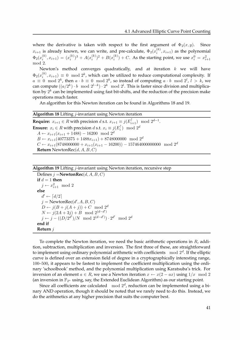
Transcript
Thesis for the Degree of Licentiate of Engineering
ISSN 0347-2809/NO 2002-13Department of MathematicsChalmers University of Technology and Göteborg UniversitySE-412 96 GöteborgSwedenTelephone +46 (0)31-772 1000
This is a thesis of the ECMI (European Consortium for Mathematicsin Industry) post-graduate program in Industrial Mathematics atChalmers University of Technology.
The work was supported by Ericsson Mobile Platform and Ericsson Radio Systems.
Matematiskt centrumGöteborg, Sweden 2002
Abstract
This thesis is concerned with security problems related to constrained devices such as mo-bile phones. Devices of this type put high demands on security solutions to be cost efficientin terms of computing power, network bandwidth and memory requirements. In this the-sis, we study elliptic curve cryptography and related computational problems in connectionwith suitable security solutions for wireless terminals. We show that elliptic curve cryptog-raphy meets high security and low cost demands for this type of devices.
In the first part of the thesis, we study efficiency problems for arithmetical operations relatedto elliptic curve cryptography. In the second part, we investigate two problems in ellipticcurve cryptography: Efficient implementation of elliptic curve arithmetic and elliptic curveparameter selection. By making an efficient implementation of elliptic curve arithmetic onan ARM micro processor, we show that elliptic curve cryptography is a very competitivealternative to traditional cryptosystems for mobile platforms. We also show how to selectparameters for elliptic curves in order to ensure the security of the cryptosystem. An efficientparameter selection algorithm enables on-the-fly curve genereation and still higher security.
Keywords: Elliptic curves, cryptography, fast arithmetic, point counting
This licentiate thesis concludes a five semester ECMI programme in applied mathematics.This programme includes a block of core courses covering several areas of applied mathe-matics and computing science and a block of specialization courses within a selected field.The final part of the programme is to work with a mathematical problem that emanates fromthe industry. The aims of the European Consortium for Mathematics in Industry are:
I To promote the use of mathematical models in industry.
I To educate industrial mathematicians to meet the growing demands for such experts.
In this thesis, we will discuss elliptic curve cryptography and its implementations. This isan important topic with many applications in modern communication where bandwidth,storage resources and computational power is constrained and strong security desired. Thespecific application we have in mind are mobile phones using the Wireless Application Pro-tocol (WAP). Mobile phones suffer all the limitations previously mentioned, and an efficientcryptographic protocol and its implementation is crucial for usability.
Our presentation is outlined as follows:
I In the first chapter, we begin by giving a brief introduction to cryptography and el-liptic curves. We also discuss the computer environments we are likely to encounter.Furthermore, we give some specifics regarding elliptic curve cryptography protocols.
I In the second chapter, we treat arithmetic over extension fields of characteristic two,and how it can be implemented efficiently.
I In chapter three, we turn to the elliptic curve group and address the issue of imple-menting arithmetic efficiently in this group.
I Lastly, in chapter four, we do an in-depth study of how to count the points on anelliptic curve, which is an important problem when constructing a secure elliptic curvecryptosystem.
1.1 Introduction to Cryptography
The area of cryptography is a broad one, hence we will only consider a small part of it.It is common to group the goals of cryptography into the four categories; Confidential-ity, Data integrity, Authentication and Non-repudiation. Of these, we will concentrate onconfidentiality—means to obstruct unauthorized parties from reading information. For anexcellent introduction to cryptography, refer to [13].
When two entities wish to communicate secretly, they can adopt many different strate-gies. For instance, they may avoid their adversaries and meet in private, they may send theirmessages in a manner that evades detection or they may send messages that, hopefully, onlythey themselves can read. We will only consider the latter of these methods.
1
Chapter 1 Introduction
1.1.1 Mathematical background
For our purposes, it will be convenient to consider information to be made up by elementsfrom some setA, called the alphabet. Elements of A can be combined into a message, whichin turn is an element of the message spaceM, consisting of possible, or allowed strings ofelements from A. When enciphering a message, we use a functionM → C, where C is theciphertext space, whose elements are strings of some alphabet, which may or may not be thesame as A. Thus, we can view the procedure of transmitting enciphered information as
Sender: fe(m) = c, m ∈M, c ∈ C,Receiver: gd(c) = m, m ∈M, c ∈ C,
where the indices e, d ∈ K are keys. For each e, d ∈ K, there exist precisely one pair fe :M→C and one gd : C →M such that the relationship above holds. If finding e knowing d, or viceversa, is easy, we say that we have a symmetric-key cipher. If finding e knowing d, or viceversa, is difficult, we say that we have a public-key cipher, or an assymetric-key cipher.
Example (Symmetric-key cipher). Let A = {A, B, C, . . ., X, Y, Z, Å, Ä, Ö} be the Swedishalphabet, and letM and C be the set of all strings of letters. Moreover, letK = Z, and fe, gd bepermutations that shift the alphabet e (d) steps to the right (left). E.g. with e = 3, fe(A) =D,fe(B) =E, . . . , fe(Z) =Ö, fe(Å) =A, . . .. Then there is a simple relationship between e and d,namely d = −e, so this cryptosystem is a symmetric-key cipher. This cipher is known as theCaesar cipher, all though the emperor himself only used one key, e = 3 (d = −3).
Our problem is to find a suitable function f so that only designated receivers can recon-struct the plaintext message m from c. To this end, we introduce the following.
Definition (Trapdoor one-way function). A trapdoor one-way function f : A → B is afunction such that for each a ∈ A it is easy to compute f(a) ∈ B, but unless given some extrainformation, it is almost infeasible to compute a ∈ A so that f(a) = b given b ∈ B. However,given the extra, trapdoor, information, it should be easy.
As an aid in our search for trapdoor one-way functions we will briefly study three im-portant and difficult problems. The first is a very famous problem that, however, is notrelated to the elliptic curve group, our main topic which will be introduced later. The othertwo problems can, and in order to see the similarities with the elliptic curve group, we useadditive notation. Especially, we use the notation [k]g = g + g + · · ·+ g (k times).
The integer factorization problem
We start out with the integer factorization problem. This is the problem of finding the primefactorization of a non-zero positive integer n, that is to write n = pm1
1 pm22 · · · p
mkk , where
p1, . . . , pk are different primes and m1, . . . mk are non-zero positive integers. There exist aplethora of algorithms to solve this, among which the (general) number field sieve appearsto be the fastest for big numbers, see e.g. [2].
The discrete logarithm problem
Let G be a finite, cyclic group, and g its generator. The discrete logarithm problem is then,given G, g and an element h ∈ G, to find an integer n such that [n]g = h.
2
1.1 Introduction to Cryptography
This appears to be an easy problem, consider for instance G = Zp (with addition), wherep is a prime. Then it is a simple matter to find n such that na = b, where a, b ∈ Zp. So, for theproblem to be a difficult one, we must choose the cyclic group G so that the isomorphismϕ : G→ Zp is hard to compute.
The Diffie-Hellman problem
As in the discrete logarithm problem, let G be a finite cyclic group, and g its generator. TheDiffie-Hellman problem is then, given two elements [m]g and [n]g in G, to find [mn]g.
Computationally, the Diffie-Hellman problem is believed to be as hard to solve as thediscrete logarithm problem. It is however evident that if it is easy to solve the discrete log-arithm problem, then it is no harder to solve the Diffie-Hellman problem. Nevertheless, itis interesting in another regard—it provides us with a nice basis for a simple cryptographicprotocol. More on this in the next section.
1.1.2 Some public-key cryptosystems
We will now give some examples of cryptosystems that utilize the problems given in theprevious section. To get started, we begin with a simple example.
Example (Diffie-Hellman key agreement). The Diffie-Hellman key agreement is a schemefor two people to share a common secret message.
1. Setup. The senderA and the receiverB agree on a finite cyclic groupG, and a generatorg. Separately and secretly, they each decide on a number, a and b respectively. Theentity (G, g, [a]g) is A’s public key, and similarly for B. Here, A’s private key is a, B’sprivate key is b.
2. Transmission. A computes [a]g and sends this to B, while B computes [b]g and sendsthis to A.
3. Their common key, that is their common secret, is [ab]g.
Remember that in order for a third party to find the secret message, the Diffie-Hellman prob-lem has to be solved. Now, it might not appear to be very useful to share a secret messagethat is not known beforehand, but this message might be used, in a specified manner, toconstruct a key for a symmetric-key cipher. In this case, it doesn’t matter what the secret keyis, as long as it is secret.
We go on with an actual encryption scheme, the first that was shown to be provablysecure, which is to say that it has been proven to be as difficult to break as its underlyingmathematical problem (unlike for instance the more well-known RSA cipher).
Example (Rabin public-key encryption). In this scheme, we have two companions, A andB, where B wants to send A a secret message m.
1. Setup. A chooses two large random primes, p ≡ 3 mod 4 and q ≡ 3 mod 4, of aboutsimilar, large sizes, and computes n = pq. A’s public key is n, while her private key is(p, q).
3
Chapter 1 Introduction
2. Encryption. To send m to A, B computes and sends c = m2 mod n, where m is repre-sented among {0, 1, . . . , n− 1}.
3. Decryption. To recover m from c, A uses (p, q) to find the four square roots m1,m2,m3
and m4 of c modulo n. They are ±x,±y mod n, if r = c(p+1)/4 mod p, s = c(q+1)/4
mod q, x = (aps + bqr) mod n, y = (aps − bqr) mod n, where ap + bq = 1. Thenm = mi for one of the four mi’s.
Breaking the Rabin cryptosystem (passively, that is without interfering with the transmis-sions) is as difficult as factoring n, see for instance [13].
Next, we give an example where the Diffie-Hellman problem enters a cryptosystem.
Example (ElGamal public-key encryption). As in the previous example, B wishes to sendA a secret message m. Unlike the previous example, we are not confined to a specific group(as long as the Diffie-Hellman problem is difficult enough to solve in the group).
1. Setup. A finite cyclic group G of order p, where p is a prime, and a generator g isagreed upon (in public). A picks a random integer a, and computes [a]g. Her publickey is (G, g, [a]g), and her private key is a.
2. Encryption. B now picks a random integer k, computes γ = [k]g, δ = m+ [k]([a]g) andsends (γ, δ) to A.
3. Decryption. Upon reception, A computes m = δ + [−a]γ.
It is plain to see that this scheme relies on the Diffie-Hellman problem (and the discretelogarithm problem in extension).
Finally, we address the issue of signatures. If A sends a message to B, she can appenda signature which allows B to verify that A was indeed the sender. First, we assume thata digest of the message has been computed, using for instance the Secure Hash Algorithm[15]. A message digest is a representative of the message computed in such a way that itshould be very difficult for two different messages to have the same digests.
Example (ElGamal signature scheme). Here we assume that we have a finite group G oforder p, where p is a prime, and a hash function h : {0, 1}∗ → Z∗
p, where {0, 1}∗ denotesthe set of all finite strings consisting of 0 and 1. We also assume that we have a functionf : G → {0, 1}∗. In the scheme, A wants to send the message m to B who in turn wants toverify that A actually sent the message.
1. Setup. A finite cyclic group G of order p, where p is prime, with generator g is selected.The sender A selects a private key a and a public key [a]g, with 1 ≤ a ≤ p− 1.
2. Signature generation. A selects a random integer k such that gcd(k, n) = 1 and thencomputes r = [k]g and s = k−1[h(m)− ah(f(r))] mod p. She then sends the signature(r, s) (along with the message m).
3. Signature verification. B computes v1 = [h(f(r))]([a]g) + [s]r and v2 = [h(m)]g. Thesignature is valid if and only if v1 = v2.
4
1.2 Introduction to Elliptic Curves
As a note for the elliptic curve group, a good f : G → {0, 1}∗ is the projection (x, y) 7→ x. Inthis case, with some modifications, the above algorithm is called ECDSA1 [7] §7,10.
1.2 Introduction to Elliptic Curves
An important topic for us is that of elliptic curves. An elliptic curve E over a field K is theset of points (x, y) ∈ K2 that satisfies an equation
y2 + a1xy + a3y = x3 + a2x2 + a4x+ a6, (1.1)
where ai ∈ K, in conjunction with a ‘point at infinity’, which will be explained later. Here,K denotes the algebraic closure of K . We will denote this set of points E(K), and when wewant to emphasize that the coefficients ofE are inK , we writeE/K . The coefficients ai havetheir indices due to historical reasons, and are standard throughout the literature.
By making the substitutions x = X/Z , y = Y/Z and clearing the denominators, (1.1)becomes
Y 2Z + a1XY Z + a3Y Z2 = X3 + a2X
2Z + a4XZ2 + a6Z
3. (1.2)
We say that the equation has been rewritten into projective coordinates, as opposed to theoriginal affine coordinates. Equation (1.2) is called the Weierstrass equation in the projectiveform (and (1.1) is the Weierstrass equation in the affine form). We denote its solutions by[X : Y : Z], where two solutions are considered equal if they are proportional. The affinepoint (x, y) corresponds to the projective triplet [X : Y : 1], which is equivalent to [X/Y :1 : 1/Y ] when Y 6= 0. If K = R, we can let Y → ∞ and get the solution [0 : 1 : 0], so thistriplet may be understood as the direction of the y-axis. We denote this triplet O, the pointat infinity. This point does not exist in the (x, y)-coordinate system, but can be imagined tolie ‘somewhere far away along the y-axis’.
More demands on E(K) are in order, as the curve must be smooth. In other words, werequire that there must be no point in E(K) where both partial derivatives with respect to xand y are zero. That is
a1y = 3x2 + 2a2y + a4, and 2y + a1x+ a3 = 0
must not hold for any (x, y) ∈ E(K), see also Figure 1.1. In characteristic 2, this meansthat a1 and a3 cannot both be equal to zero. Non-singular curves with a1 = 0 are calledsupersingular, whereas curves with a3 = 0 are called non-supersingular. For cryptographicreasons, we will almost exclusively be interested in non-supersingular elliptic curves. Theequation (1.2), that describes an elliptic curve can be rewritten without changing the form(1.1) using the substitution
x = u2x′ + r, y = u3y′ + u2sx′ + t, (1.3)
where u ∈ K∗, r, s, t ∈ K . A substitution of this form is called twisting. In our favorite case,fields of characteristic 2, if a1 6= 0, the substitution
x = a21x
′ + a3/a1, y = a31y
′ + (a1a4 + a23)/a
31
1In ECDSA, the signature is (s, f(r)), and to verify the signature, we compute q = s−1 mod n and q1 =q · h(m) mod n, h2 = q · f(r) mod n. Then we compute r′ = [h1]g + [h2]([a]g). The signature is valid iff(r′) = f(r).
5
Chapter 1 Introduction
−1.5 −1 −0.5 0 0.5 1 1.5 2−1.5
−1
−0.5
0
0.5
1
1.5
x
y
−1.5 −1 −0.5 0 0.5 1 1.5 2−1.5
−1
−0.5
0
0.5
1
1.5
x
y
Figure 1.1: To the left is the non-singular elliptic curve y2 = x3 − x over R, and to the right is thesingular curve y2 = x3, also over R.
gives us an equation
y2 + xy = x3 + a2x2 + a6. (1.4)
Similarly, if a1 = 0 (and a3 6= 0), the substitution x = x′ + a2, y = y′ gives an equationy2 + a3y = x3 + a4x+ a6.
For an elliptic curve E, we define the discriminant ∆(E) and the so-called j-invariantj(E). In the case, when K = F2n , and (1.4) is an equation for the elliptic curve, the discrim-inant ∆(E) = a6 and j(E) = 1/a6. The j-invariant is invariant in the sense that two curveswith the same j-invariant can be transformed into each other using the (1.3). It should benoted that all non-supersingular curves have a non-zero j-invariant, see [21], §III for moredetails.
1.2.1 The group law
The property that perhaps is the most important reason why elliptic curves are used in cryp-tography is that they can be supplied with a group structure turning the set of their pointsinto a group. To see how it can be defined, letE be an elliptic curve over R for the remainderof this section unless otherwise stated.
Recall that the equation for an elliptic curve is a cubic in the x-coordinate. This meansthat a line in the plane intersects an elliptic curve at most three times. In fact, if the line isnot a tangent to the curve nor vertical, it will intersect the curve exactly three times. This isthe basis for the group law. Let P = (xP , yP ) and Q = (xQ, yQ) be points on E.
1. If P = O, the point at infinity, let P +Q = O +Q = Q.
2. If (xP , yP ) = (xQ,−xQ), let P +Q = O.
3. If xP 6= xQ, then let −(P + Q) be the third point of intersection with E on the linethrough P and Q, see also the left graph in Figure 1.2.
6
1.2 Introduction to Elliptic Curves
−1.5 −1 −0.5 0 0.5 1 1.5 2−1.5
−1
−0.5
0
0.5
1
1.5
x
y
PSfrag replacements
P
Q
−(P +Q)
P +Q
−1.5 −1 −0.5 0 0.5 1 1.5 2−1.5
−1
−0.5
0
0.5
1
1.5
x
y
PSfrag replacements
PQ
−(P +Q)
P +Q
P −[2]P
[2]P
Figure 1.2: The group law on the elliptic curve y2 = x3−x over R. To the left the addition law P +Qis illustrated, to the right the doubling law P + P = [2]P .
4. IfP = Q, then take the tangent line to the curve atP , and let−(P+Q) = −[2]P = −[2]Qbe the other point of intersection of this line with E, see also the right graph in Figure1.2.
To derive formulae for these rules, let E have the equation
y2 = x3 + ax+ b
(every elliptic curve over a field of characteristic not equal to 2 or 3 can be written in thisform), and let R = P + Q = (xR, yR). The line through P and Q (P 6= Q, case 3 above) is ofthe form y = αx + β, where α = (yP − yQ)/(xP − xQ) and β = yP − αxP . Now, a point onthe line (x, αx + β) intersects E if (αx + β)2 = x3 + ax + b, or x3 − (αx + β)2 + ax+ b = 0.We already now that (xP , αxP + β) and (xQ, αxQ + β) solve this cubic, which means thatα2 = xP + xQ + xR, or xR = α2 − xP − xQ, so
xR = α2 − xP − xQ =
(
yP − yQ
xP − xQ
)2
− xP − xQ,
yR = −(αxR + β) =
(
yP − yQ
xP − xQ
)
(xP − xR)− yP .
In the fourth case, if P = Q, we take α as dy/dx of E at P . Taking the implicit derivativegives α = dy/dx = (3x2
P + a)/2yP , so
xR = α2 − 2xP =
(
3xP + a
2yP
)2
− 2xP ,
yR = −(αxP + β) =
(
3xP + a
2yP
)
(xP − xR)− yP .
We note, however, that the two formulae are only valid if charK 6= 2, 3. If P = Q we writeR = [2]P , and call this computation a point doubling. Repeated additions and doublingsgive us [k]P , what we call scalar multiplication.
7
Chapter 1 Introduction
In characteristic two, the formulae for non-supersingular curves become
xR = λ2 + λ+ xP + xQ + a2,
yR = λ[xR + xP ] + xR + yP ),
λ =
{
yP +yQ
xP +xQ, if P 6= R,
xP + yP /xP , if P = R.
To find this, first repeat the process above for the general curve equation (1.1), and then leta1 = 1, a3 = a4 = 0.
1.2.2 The number of points
In this section, we will introduce the notion of point counting, and give some basic prop-erties. Further information is found in section 4.1. An excellent pre-1999 account for pointcounting can be found in [19]. A description of more recent advances can be found in Chap-ter 4.
By the number of K-rational points on an elliptic curve E, we mean the number of(x, y) ∈ K2 that satisfy the elliptic curve equation. We will denote this number N , andsometimes #E(K).
If E/Fq is an elliptic curve, it is also defined over the extension Fqr , and if the number ofpoints to E over Fq is N , then we denote by Nr = #E(Fqr) the number of points of E overFqr , where N1 = N . Now, define the zeta-function
Z(E/Fq;T ) = e∑
NrT r/r,
where the sum is over all positive r = 1, 2, . . .. This function turns out to have a surprisinglysimple form:
Theorem (The Weil Conjecture for Elliptic Curves). Let E be an elliptic curve defined over thefield Fq. Then there is an a ∈ Z such that
Z(E/Fq;T ) =1− aT + qT 2
(1− T )(1− qT ).
Moreover, N = q + 1− a, and a2 ≤ 4q.
See [21], §V.2, for a proof and further information. We note that from this formula it iseasy to obtain Nr if we know N (by derivating r times with respect to T ). However, curvesE/Fq, where q is small, are considered to be cryptographically weak if q is small, and will beof no interest to us.
An important and immediate consequence of this result is the following bound for thenumber of points on an elliptic curve:
Theorem (Hasse’s Theorem). Let E be an elliptic curve defined over Fq, and let N be the numberof points in E(Fq). Then,
|q + 1−N | ≤ 2√q
8
1.3 Efficiency and the Environment
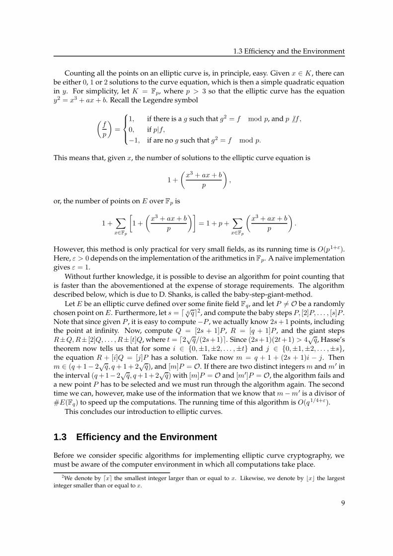
Counting all the points on an elliptic curve is, in principle, easy. Given x ∈ K , there canbe either 0, 1 or 2 solutions to the curve equation, which is then a simple quadratic equationin y. For simplicity, let K = Fp, where p > 3 so that the elliptic curve has the equationy2 = x3 + ax+ b. Recall the Legendre symbol
(
f
p
)
=
1, if there is a g such that g2 = f mod p, and p 6 |f,0, if p|f,−1, if are no g such that g2 = f mod p.
This means that, given x, the number of solutions to the elliptic curve equation is
1 +
(
x3 + ax+ b
p
)
,
or, the number of points on E over Fp is
1 +∑
x∈Fp
[
1 +
(
x3 + ax+ b
p
)]
= 1 + p+∑
x∈Fp
(
x3 + ax+ b
p
)
.
However, this method is only practical for very small fields, as its running time is O(p1+ε).Here, ε > 0 depends on the implementation of the arithmetics in Fp. A naïve implementationgives ε = 1.
Without further knowledge, it is possible to devise an algorithm for point counting thatis faster than the abovementioned at the expense of storage requirements. The algorithmdescribed below, which is due to D. Shanks, is called the baby-step-giant-method.
Let E be an elliptic curve defined over some finite field Fq, and let P 6= O be a randomlychosen point onE. Furthermore, let s = d 4
√qe2, and compute the baby stepsP, [2]P, . . . , [s]P .
Note that since given P , it is easy to compute−P , we actually know 2s+1 points, includingthe point at infinity. Now, compute Q = [2s + 1]P , R = [q + 1]P , and the giant stepsR±Q,R± [2]Q, . . . , R± [t]Q, where t = d2√q/(2s+1)e. Since (2s+1)(2t+1) > 4
√q, Hasse’s
theorem now tells us that for some i ∈ {0,±1,±2, . . . ,±t} and j ∈ {0,±1,±2, . . . ,±s},the equation R + [i]Q = [j]P has a solution. Take now m = q + 1 + (2s + 1)i − j. Thenm ∈ (q+ 1− 2
√q, q+ 1 + 2
√q), and [m]P = O. If there are two distinct integersm and m′ in
the interval (q+1−2√q, q+1+2
√q) with [m]P = O and [m′]P = O, the algorithm fails and
a new point P has to be selected and we must run through the algorithm again. The secondtime we can, however, make use of the information that we know that m−m′ is a divisor of#E(Fq) to speed up the computations. The running time of this algorithm is O(q1/4+ε).
This concludes our introduction to elliptic curves.
1.3 Efficiency and the Environment
Before we consider specific algorithms for implementing elliptic curve cryptography, wemust be aware of the computer environment in which all computations take place.
2We denote by dxe the smallest integer larger than or equal to x. Likewise, we denote by bxc the largestinteger smaller than or equal to x.
9
Chapter 1 Introduction
1.3.1 Memory structure
In a modern computer, there is a hierarchy of storage memory. For instance, a PC usuallyhas a hard disk, primary memory, an on chip cache and two additional caches in the centralprocessing unit (CPU). The standard rule is that the closer memory is to the processor, thefaster it is.
The fastest memory is that inside the processor. First, and foremost, a processor has anumber of registers, which is where the actual computations take place. At the next higherlevel, a modern processor has two cache memories, one for instructions to be executed, andone for recently used, or to be used, data. The second level cache resides outside of theprocessor, but usually runs at a higher speed than the ordinary memory, though it commonlyis not as large.
Normally, if an instruction reads data from memory, that and adjacent data is read tothe cache, usually a multiple of 2 bytes. Since several bytes of data is read, a first memoryfetch is usually quite slow. Subsequent reads from that same memory region can, however,be processed very fast. Therefore it is important to keep data dense, aligned to the specificmultiple of 2 that the system architecture uses, and avoid random accesses instead of sequen-tial. The same applies for instructions; especially important are frequently used instructions,commonly residing inside loops.
1.3.2 The central processing unit
Where memory structure does not differ much between platforms except for sizes, the work-ings of the CPU do. In personal computers nowadays there are two varieties of processorfamilies, reduced instruction set computers (RISC) and complex instruction set computers(CISC). As their names indicate, the two families differ in how many instructions are avail-able and how complex these instructions are. Typically, RISC processors, such as the onesfound in many modern mobile phones, have two types of instructions—moving data be-tween the memory and the registers of the CPU, and doing calculations on data in the reg-isters. In comparison, in a CISC processor, such as the ones found in many modern PC’s,instructions can often manipulate data regardless of its location.
1.4 Elliptic Curve Cryptosystems
In Section 1.1.2, we gave four examples of public-key cryptosystems three of which are validfor any cyclic group. These three cryptosystems are in fact the most commonly used forthe elliptic curve group, although of most importance are the Diffie-Hellman key agreementand the ElGamal signature scheme. The reason for this is, that compared to symmetric-key ciphers, public-key ciphers are computationally more demanding for the same securitylevel. However, as symmetric-key ciphers require that both parties know the same secretkey, public-key ciphers are generally used to transmit the secret key securely, after which theactual message transmission uses the symmetric-key cipher.
Why is it then, that we should use the elliptic curve group instead of an ordinary cyclicgroup such as Z∗
p which is easier to implement and use? The reason is, of course, security.The best known algorithm for solving the discrete logarithm problem in Z∗
p is, as indicated
10
1.4 Elliptic Curve Cryptosystems
earlier, the number field sieve, which has a running time proportional to
L(p) = e(1.992+o(1))(ln p)1/3(ln ln p)2/3,
where o(1) → 0 as p → ∞. This means that the number field sieve is sub-exponential. Tosolve the discrete logarithm in the elliptic curve group, however, no sub-exponential algo-rithm is known. The best general method to date is Pollard’s ρ-method which has runningtime O(0.88
√n) group operations, where n is the largest prime divisor of the number of
points on the elliptic curve. It should be noted that there are certain classes of curves forwhich there are sub-exponential algorithms, curves which should therefore be avoided, seeSection 4.2.
In practical terms, these differences in running time, give implication in how large weneed the groups to be, i.e. the key sizes. If we want our information to be secure for, say20 years, until 2022, we should select an elliptic curve defined over Fq where log2 q ≈ 164[9], which means that our public key can be represented using a number which is about165 bits (we need only store the x-coordinate and one extra bit which tells which of the twoy-coordinates we use).
For a discrete logarithm cryptosystem over Z∗p, we’ll need about 2000 bits to achieve the
same security. This is a considerable difference in terms of storage space, the arithmetic andtransmission costs, and is the main reason why elliptic curve cryptography is interestingtoday.
11
Chapter 2
Efficient Arithmetics in F2n
In this chapter, we will discuss how to perform the basic operations in F2n efficiently. Asmentioned previously, what is most efficient will depend heavily on the computer platform,but in this chapter no assumptions will be made regarding which computer platform is used.We will start with a discussion of different ways to represent the elements of F2n since thealgorithms for addition/subtraction, multiplication, inversion and exponentiation will differdue to the representation. Only thereafter will the specific algorithms be put under scrutiny.
2.1 Field Representation
We first turn our attention to the question ’How do we represent an element a ∈ F2n in acomputer so that we can perform efficient computations with it?’
2.1.1 Polynomial bases
Using a polynomial basis is the classical way of handling an extension field such as F2n . Inthis case, we write F2nas F2[X]/(p(x)), where p(x) is an irreducible polynomial of degree n,so that each a ∈ F2n is a polynomial modulo p(x) with binary coefficients, i.e. a ∈ F2n iswritten as
a = a0 + a1x+ · · ·+ an−1xn−1, ai ∈ {0, 1}
which using the basis {1, x, x2, . . . , xn−1} can be represented as the vector a =(a0, a1, a2, . . . , an−1). In a computer environment, this means that we let each ai be one bit,with, preferably a0 the least significant. The coefficients are then grouped into groups of,usually, 32 or 64 depending on the computer architecture.
The polynomial representation lends itself to computations rather straightforward man-ner. We now how to add, multiply and divide two polynomials from high school, but maybenot how to do it quickly. From experience, we know that multiplication and division willbe the most cumbersome operations. Addition is simple, since all coefficients are modulo2, and can be implemented with the logical exclusive-or operation. When multiplying anddividing, since we calculate modulo p(x), care has to be taken to choose the reduction poly-nomial p(x) so that these operations can be performed quickly. In practice this means thatthe weight of p(x) should be small, preferably a trinomial.
13
Chapter 2 Efficient Arithmetics in F2n
2.1.2 Normal bases
In a normal basis, we start with an irreducible polynomial p(x), and one of its roots θ ∈ F2n .The basis is of the form
{θ, θ2, θ22, θ23
, . . . , θ2n−1},
where all the elements of the basis satisfy p(θ2i) = 0. We see that squaring becomes very
simple—just shift your vector a = (a0, a1, . . . , an−1), where again ai ∈ {0, 1}, one step to theleft, whereas multiplication and inversion is more difficult. There are two special cases ofnormal bases which are worth mentioning, both are called Optimal Normal Bases (ONB).
Optimal Normal Bases
For certain n, we can construct a normal basis that yields faster multiplication and inversion.This happens when for all 0 ≤ i1 6= i2 ≤ n−1 there exist j1, j2 such that θ2i1+2i2 = θ2j1 +θ2j2 .An ONB can be constructed when
Type I n+ 1 is a prime p and 2 is a primitive root modulo p.
Type II 2n+ 1 is a prime p and either
1. 2 is primitive modulo p, or
2. p ≡ 3 (mod 4), and the multiplicative order of 2 modulo p is n.
Type I ONB’s are attractive since then θ is a root of p(x) = xn +xn−1 + · · ·+x+1, and itis possible to treat elements as polynomials modulo (x+ 1)f(x) = xn+1 + 1. A changeof bases between the polynomial basis and the normal basis can be performed using1 = θ + θ2 + · · ·+ θn.
The type II representation can also be given similar characteristics. In this case, we canwrite θ = γ + γ−1, where γ is a pth root of unity in F2n . It is now possible to calculateusing polynomials if we take the polynomials to be
a(x) =2n∑
i=1
aixi,
where ai = ap−i (a so called palindromic polynomial), and multiplication is carried outmodulo xp−1. A change of bases to the ONB is then done through a(γ) =
∑n−1j=0 a2jθ2j
.See also [6].
2.1.3 Subfield bases
A special case of F2n is when n = n1n2 where n1, n2 ≥ 1, and n1 is rather small, say 16or below. It is then possible to view F2n as Fqn2 , where q = 2n1 , and the elements of F2n
are polynomials with coefficients in Fn1 . The operations in the subfield can be tabulatedand computations severely sped up. However, we will not concern ourselves with these, aselliptic curve cryptosystems built on such fields have been shown to be weak, see Section4.2.
14
2.2 Multiplication
2.2 Multiplication
We now move on to the problem of computing c = ab, when a, b ∈ F2n . Obviously, ourtactics will differ depending on the representation, and we will confine ourselves to onlystudy polynomial bases, as experience has shown these to be most efficient.
2.2.1 Schoolbook multiplication
Given a(x) =∑n−1
i=0 aixi, b(x) =
∑n−1i=0 bix
i, we can calculate c(x) = a(x)b(x) through thedouble sum
c(x) =2n−2∑
i=0
(
∑
k+l=i
akbl
)
xi,
that is ci =∑i
k=0 akbi−k, where only indices satisfying 0 ≤ i, i − k < n are included. Thisprocedure is summarized in Algorithm 1. Note that we don’t do the required reductionmodulo p(x).
Algorithm 1 Schoolbook multiplication
Require: a(x) =∑n−1
0 aixi, b(x) =
∑n−10 bix
i
Ensure: c(x) = a(x)b(x)for i = 0 to 2n− 2 do
for k = 0 to i do
if 0 ≤ i− k, k < n then
ci ← ci + akbi−k
end if
end for
end for
2.2.2 Comb methods
One idea that turns out to be useful when multiplying is to use previous results wheneverpossible. First, we write a as a vector, a = (an−1, an−2, . . . , a1, a0), and write its division intoW -tuplets as A = (A[k], A[k − 1], . . . , A[0]), where A[i] = (aW (i+1)−1, . . . , aWi) is called aword. Here we chose W in order to maximize speed, which is dependent on the computerarchitecture. Usually we take W to be equal to 32. We also define A{j} = (A[k], . . . , A[j +1], A[j]) (thus A = A{0}).
First, we notice that we can write the polynomial product as
The idea behind the comb methods is based on the observation that if we have computedb(x)·xk for some k, then it is very easy to compute b(x)·xWj+k by simply appending 0-words
15
Chapter 2 Efficient Arithmetics in F2n
at the end of the vector representing b(x) · xk. This is equivalent with writing the product as
a(x)b(x) =
W−1∑
k=0
bn/W c∑
j=0
xWj+kaWj+kb(x)
,
where the inner sum can be calculated quickly, as before mentioned. An example might bein order: let a = 010|110, b = 001|101 (so c = 011|111|110) (’|’ indicates W = 3 separation).Now
The comb methods can be implemented in several ways. Algorithm 2 is the one outlinedin the example above, whereas Algorithm 3 is a slight modification.
Algorithm 2 The right-to-left comb method
Require: a(x) =∑n−1
0 aixi, b(x) =
∑n−10 bix
i
Ensure: c(x) = a(x)b(x)C ← 0for k = 0 to W − 1 do
for j = 0 to bn/W c do
if the kth bit of A[j] is 1 then
C{j} ← C{j}+Bend if
end for
if k 6= 31 then
B ← B · xend if
end for
We notice that Algorithm 2 is faster than Algorithm 3, since in the latter, C is shiftedinstead of B, where C is twice as large as B. But, we do include Algorithm 3 due to the factthat it may be sped up using some overhead storage. If w|W , we can pre-compute u(x)b(x)for all polynomials u(x) of degree less than w, put them in a table, and shorten the outerloop. This is done in Algorithm 4.
2.2.3 Karatsuba multiplication and relatives
The multiplication methods described above all have in common that they require O(n2)multiplications (of coefficients or by x). That is not a necessary trait, as we will now show.When multiplying two first degree polynomials, the ordinary way, we get
Ensure: c(x) = a(x)b(x)C ← 0for k = W − 1 downto 0 do
for j = 0 to bn/W c do
if the kth bit of A[j] is 1 then
C{j} ← C{j}+Bend if
end for
if k 6= 0 then
C ← C · xend if
end for
Algorithm 4 The left-to-right comb method with windows
Require: a(x) =∑n−1
0 aixi, b(x) =
∑n−10 bix
i
Ensure: c(x) = a(x)b(x)Pre-compute Bu = u(x)b(x) for all polynomials u(x) of degree less than or equal to w − 1C ← 0for k = W/w − 1 downto 0 do
for j = 0 to bn/W c doLet u = (u3, u2, u1, u0) where ui is bit (wk + i) of A[j].C{j} ← C{j}+Bu.
end for
if k 6= 0 then
C ← C · xw
end if
end for
17
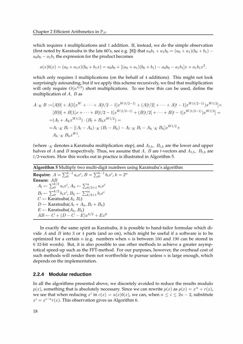
Chapter 2 Efficient Arithmetics in F2n
which requires 4 multiplications and 1 addition. If, instead, we do the simple observation(first noted by Karatsuba in the late 60’s, see e.g. [8]) that a0b1 + a1b0 = (a0 + a1)(b0 + b1)−a0b0 − a1b1 the expression for the product becomes
which only requires 3 multiplications (on the behalf of 4 additions). This might not looksurprisingly astounding, but if we apply this scheme recursively, we find that multiplicationwill only require O(n4/3) short multiplications. To see how this can be used, define themultiplication of A, B as
(where ·K denotes a Karatsuba multiplication step), and Al,h, Bl,h are the lower and upperhalves of A and B respectively. Thus, we assume that A, B are t-vectors and Al,h, Bl,h aret/2-vectors. How this works out in practice is illustrated in Algorithm 5.
Algorithm 5 Multiply two multi-digit numbers using Karatsuba’s algorithm
Require: A =∑k−1
0 aixi, B =
∑k−10 bix
i, k = 2n
Ensure: ABAl ←
∑k/20 aix
i, Ah ←∑n
k/2+1 aixi
Bl ←∑k/2
0 bixi, Bh ←
∑mk/2+1 bix
i
C ← Karatsuba(Al, Bl)D ← Karatsuba(Al +Ah, Bl +Bh)E ← Karatsuba(Ah, Bh)AB ← C + (D − C −E)xk/2 +Exk
In exactly the same spirit as Karatsuba, it is possible to hand-tailor formulae which di-vide A and B into 3 or 4 parts (and so on), which might be useful if a software is to beoptimized for a certain n (e.g. numbers when n is between 160 and 190 can be stored in6 32-bit words). But, it is also possible to use other methods to achieve a greater asymp-totical speed-up such as the FFT-method. For our purposes, however, the overhead cost ofsuch methods will render them not worthwhile to pursue unless n is large enough, whichdepends on the implementation.
2.2.4 Modular reduction
In all the algorithms presented above, we discretely avoided to reduce the results modulop(x), something that is absolutely necessary. Since we can rewrite p(x) as p(x) = xn + r(x),we see that when reducing xi in c(x) = a(x)b(x), we can, when n ≤ i ≤ 2n − 2, substitutexi = xi−nr(x). This observation gives us Algorithm 6.
18
2.3 Squaring
Algorithm 6 Trivial modular reduction
Require: c(x) =∑2n−2
0 cixi, p(x) = xn + r(x)
Ensure: c(x) (mod p(x))for i from 2n− 2 to n do
if ci = 1 then
ci ← 0c(x)← c(x) + xn−ir(x)
end if
end for
We note three things about this algorithm: Firstly, the lower the degree of r(x) (or if theterms are close to each other), the better. Secondly, the lower the weight of r(x) the betterand lastly, it might be worthwhile to precompute xjr(x) for 0 ≤ j ≤ 31.
It is possible to speed this algorithm up, by working with groups of W coefficients ata time, where W is typically 32. To see how this can be done, consider the substitutionxa → xa−l for W a’s, with l = Wm+ n, where 0 ≤ n < W :
xWk+W−1 → xW−1xW (k−m)−n,
xWk+W−2 → xW−2xW (k−m)−n,
...
xWk → x0xW (k−m)−n.
Since W − i− n = 0 for some i, this can be rewritten as
xWk+W−1 → xW−1xW (k−m)−n,
xWk+W−2 → xW−2xW (k−m)−n,...
xWk+W−i → xW−ixW (k−m−1)+(W−n),
xWk+W−i−1 → xW−i−1xW (k−m−1)+(W−n),...
xWk → x0xW (k−m−1)+(W−n).
(2.1)
This means that in a computer, where usually W = 32, we can implement this substitutionusing a bit-shift of n to the right or W − n to the left. The reason for the division at i is that aright shift larger than W becomes zero in the computer.
For a full modular reduction, write the reduction polynomial as p(x) = xp1 + · · · + xpk ,let li = p1 − pi+1 for i = 1, . . . , k − 1 and write li = Wmi + ni with 0 ≤ ni < W and do thesubstitution (2.1) k − 1 times. For details, see Algorithm 7.
2.3 Squaring
The problem of squaring is to calculate a2 = a · a. In characteristic two, squaring is particu-larly simple as (x+y)2 = x2+y2, giving a2(x) =
∑
aix2i. Thus we have to insert a 0 between
19
Chapter 2 Efficient Arithmetics in F2n
Algorithm 7 Windowed modular reduction
Require: c(x) =∑2n−1
0 cixi, p(x) = xp1 + · · · + xpl , a window size W = 2d, usually 32.
Ensure: c(x) (mod p(x))Precomputation. Let Wj + nj,i = p1 − pi+1, 0 ≤ nj,i < W and oj+1,i = 32 − nj,i. Letdj = #{i : nj,i have been defined} and J = {j : dj > 0}. Further, let M2 = 2k − 1, wherek is the smallest k s.t. 2k − 1 ≥ [p1 AND (W − 1)] and M1 = NOT M2 be bit-masks. Asbefore, denote by C[i] = (cWi+W−1, . . . , cWi+1, cWi).for i from d[(2n− 1)/W e to dn1e do
A← C[i]for j ∈ J do
C[i− j]← C[i− j] +∑
k(A >> nj,k) +∑
k(A << oj,k)end for
end for
A← C[bn1/W c] AND M1
for j ∈ J ∩ {j : bn1/W c >= j} do
C[i− j]← C[i− j] +∑
k(A >> nj,k) +∑
k(A << oj,k)end for
C[bn1c]← C[bn1c] AND M2
every bit in the representation of a(x). If we allow ourselves some storage for a table, we cando this even faster, as in Algorithm 8.
Algorithm 8 Squaring (W = 32)
Require: a(x) =∑n−1
0 aixi
Ensure: a2(x)Precompute say b(x) = (0, x3, 0, x2, 0, x1, 0, x0) for every nibble (x4x3x2x1x0).for i from 0 to bn/32e do
Let A[i] = (u7, u6, u5, . . . , u0) where ui is a nibble.C[2i]← (b(u3), b(u2), b(u1), b(u0)), C[2i+ 1]← (b(u7), b(u6), b(u5), b(u4))
end for
2.4 Inversion
Next, we turn to the problem of inverting the elements of F2n . Here too, we confine ourselvesto the polynomial basis representation of F2n .
2.4.1 The Extended Euclidean Algorithm
The traditional way of inverting a polynomial f(x) (mod p(x)) is to use the Extended Eu-clidean Algorithm for polynomials, which gives us polynomials g, h such that f(x)g(x) +h(x)p(x) = 1, where g(x) = f(x)−1 (mod p(x)). This algorithm is on display in Algorithm 9.
20
2.4 Inversion
Algorithm 9 Extended Euclidean Algorithm for inversion
Require: a(x) =∑n−1
0 aixi, p(x)
Ensure: a(x)−1 (mod p(x))b← 1, c← 0, v ← p. u← awhile deg(u) 6= 0 do
j ← deg(u)− deg(v)if j < 0 then
u↔ v, b↔ c, j ↔ −jend if
u← u+ xjv, b← b+ xjcend while
2.4.2 The Almost-Inverse Algorithm
An alternative to the algorithm above is the Almost-Inverse Algorithm (AIA) [20]. Insteadof returning g, h such that f(x)g(x) + h(x)p(x) = 1, AIA returns f, g such that f(x)g(x) +h(x)p(x) = xk (mod p(x)).
Algorithm 10 Almost-Inverse Algorithm
Require: a(x) =∑n−1
0 aixi, p(x)
Ensure: b(x) = xka(x)−1 (mod p(x))1: b← 1, c← 0, v ← p, u← a2: while x divides u do
3: u← u/x, c← cx, k ← k + 14: end while
5: if u = 1 then
6: return (b, k)7: end if
8: if deg(u) < deg(v) then
9: u↔ v, b↔ c10: end if
11: u← u+ v, b← b+ c12: goto step 2.
On the average, AIA is expected to need fewer iterations, as is evident from the while-loop. After the algorithm has been performed, we will need to reduce the result, which canbe done as follows: Define s to be the smallest i ≥ 1 such that pi = 1, where p(x) =
∑
pixi,
and let b be such that b(x)a(x) = xk, and b′ be the polynomial formed by the s rightmostbits of b. Then let b′′ = (b′f + b)/xs (which is a non-rational function) and continue withb ← b′′. We notice that if s ≥ W , this process is faster and such reduction polynomials aremore suited for AIA than others.
2.4.3 The Modified Almost-Inverse Algorithm
The AIA can be modified to the extent that the final reduction step is removed by integratingthe reduction into the first while-loop. This is done in Algorithm 11.
21
Chapter 2 Efficient Arithmetics in F2n
Algorithm 11 Modified Almost-Inverse Algorithm
Require: a(x) =∑n−1
0 aixi, p(x)
Ensure: a(x)−1 (mod p(x))1: b← 1, c← 0, v ← p, u← a2: while x divides u do
3: u← u/x4: if x divides b then
5: b← b/x6: else
7: b← (b+ p)/x8: end if
9: end while
10: if u = 1 then11: return (b)12: end if
13: if deg(u) < deg(v) then
14: u↔ v, b↔ c15: end if
16: u← u+ v, b← b+ c17: goto step 2.
In comparison with AIA, MAIA is faster if s is small, but might be slower when s is large,so it depends on the reduction polynomial (and the implementation).
2.5 Summary
We give a few timings of an implementation made in assembler and C for the ARM 7TDMIprocessor in Table 2.1.
Table 2.1: Timings of arithmetic routines for an 10MHz ARM 7TDMI processor (emulated) on F2163 .
We see from the table that inversion is more than 10 times slower than multiplication.In the implementation, all basic routines except for reduction were implemented in assem-bler, and no special optimizations were made with regard to the specific field F2163 . Also,execution speed on the ARM processor suffers when data is fetched and stored to memory,so squaring for instance would benefit with a larger look-up table than what was used (16values stored), but it would require more storage space, which is not abundant.
22
Chapter 3
Efficient Elliptic Curve Arithmetics
In this chapter, we will discuss how to do calculations on elliptic curve groups, definedover a finite field of characteristic two, as efficiently as possible. We will also try to, whenappropriate, link this discussion to that of the previous chapter, as they are dependent oneach other. In this chapter we will always consider elliptic curves defined over F2n .
3.1 Coordinate Representations
In this first section, we will look into various ways of representing the points of ellipticcurves. As a rule, the (ordinary) affine coordinates will be denoted x and y, and rules willbe given that transform the other variants back to these. In general, the different forms ofprojective coordinates (which use a third Z-coordinate) can be obtained by simply settingthe extra coordinate values to 1.
3.1.1 Affine coordinates
We recall that in affine coordinates, the elliptic curve equation in characteristic two (withj 6= 0) may be given as
E : y2 + xy = x3 +Bx2 +A. (3.1)
We also recall the group law algorithms in affine coordinates. Let Pi = (xi, yi) ∈ E. Then
Further, we can try to calculate the number of finite field operations that is needed to per-form the computations above. When adding two distinct points, we thus need 9 additions,2 multiplications, 1 squaring and 1 inversion to add two points, whereas a point doublingneeds 8 additions, 2 multiplications and 1 inversion in F2n . From now on, we will denotethe number of operations needed for point doubling as t2(affine) ≤ 9A+ 2M + 1S + 1I andthe number of operations needed for point addition as t+(affine) ≤ 8A + 2M + 1I whereA,M,S, I stands for addition, multiplication, squaring and inversion respectively.
23
Chapter 3 Efficient Elliptic Curve Arithmetics
Projective coordinates
As mentioned before, an other natural way of describing the points on the curve is to usethe projective coordinates (X,Y,Z), where the point at infinity is represented as (0, 1, 0). Totransfer to projective coordinates, set x = X/Z and y = Y/Z to get the curve equation
E : Y 2Z +XY Z = X3 +BX2Z +AZ3. (3.2)
We note that this will enable us to do curve calculations without any field inversions.To find the addition and doubling formulae in these coordinates, we make the substitu-
tions xi ← Xi/Zi and yi ← Yi/Zi in the formulae for the affine coordinates. Then we try tosimplify the formulae inserting temporary variables wherever possible to reduce the numberof operations. For addition, we get
X3 = λ2λ3,
Y3 = X1Z2λ1λ22 + λ1λ3 + λ2λ3 + Y1Z2λ
22,
Z3 = Z1Z2λ32,
where
λ1 =
{
Y1Z2 + Y2Z1, if P1 6= P2,
X21 + Y1Z1, if P1 = P2,
λ2 =
{
X1Z2 +X2Z1, if P1 6= P2,
X1Z1, if P1 = P2,
λ3 = Z1Z2λ21 + Z1Z2λ1λ2 + λ3
2 +BZ1Z2λ22.
This means that t+(projective) ≤ 8A+ 16M + 2S and t2(projective) ≤ 7A+ 14M + 3S
Jacobian projective coordinates
Now, we start looking into ‘unnatural’ choices of coordinate substitutions that are merelyconstructs to enhance the speed of computation. The, historically, first and foremost of thesewere the Jacobian projective coordinates (X,Y,Z) which are found through the substitutionsx = X/Z2, y = Y/Z3. In this case, the elliptic curve equation transforms into
These formulae yield t+(jacobian) ≤ 7A + 15M + 5S and t2(jacobian) ≤ 4A + 5M + 5S.See also [7]. We conclude that these coordinates give faster formulae for both addition andmultiplication than ordinary projective coordinates but, unlike [7] proclaims, there exists afaster algorithm as we will soon see.
Chudnovsky Jacobian coordinates
Another construct, due to Chudnovsky, reaches speed on the behalf of storage memory re-quirements. Here, we represent the points as the quintuplet (X,Y,Z, Z 2, Z3), where, as inthe ordinary Jacobian coordinates, x = X/Z2, y = Y/Z3. The speed-up versus Jacobian co-ordinates is, of course, due to the fact that we won’t have to calculate the square or the cubeof Z .
We don’t list the formulae for addition and doubling here, as they are identical to those inthe previous section, only we never need calculate Z 2
i , Z3i for i = 1, 2. The gains are modest—
we save 1M + 1S when adding but loose that same time when doubling, leading us to theconclusion that the Chudnovsky representation is appropriate when more additions thandoublings are performed.
López-Dahab projective coordinates
The last set of coordinate representation we look into are due to López and Dahab [10]. Theypropose that we represent points as the triplets (X,Y,Z), where x = X/Z, y = Y/Z 2. In thiscase, the elliptic curve equation transforms into
E : Y 2 +XY Z = X3 +BX2Z2 +AZ4. (3.4)
The first fact used here is that, using the affine elliptic curve equation (Equation (3.1)), theaffine doubling formula can be rewritten as
x2 = λ2 + λ+B =
(
x21 + y1
x1
)2
+x2
1 + y1
x1+B =
x41 + y2
1 + x31 + x1y1
x21
+B =
=x4
1 +Bx21 +A
x21
+B = x21 +
A
x21
,
y2 = x21 + (x1 +
y1
x1)x2 + x2.
(This reformulation means that two inversions are necessary, so it is rather slow.) Rewritingthese formulae using the substitution into the López-Dahab coordinates yields the doublingformula
Z3 = X21Z
21
X3 = X41 +AZ4
1
Y3 = AZ41Z2 +X2(BZ2 + Y 2
1 +AZ41 ),
25
Chapter 3 Efficient Elliptic Curve Arithmetics
where t2(ld) ≤ 4A+ 5M + 5S. The addition formula becomes
A0 = Y2 · Z21 , D = B0 +B1, H = C · F,
A1 = Y1 · Z22 , E = Z1 · Z2, X3 = C2 +H +G,
B0 = X2 · Z1, F = D · E, I = D2 · B0 · E +X3,B1 = X1 · Z2, Z3 = F 2, J = D2 · A0 +X3,C = A0 +A1, G = D2 · (F +B · E2), Y3 = H · I + Z3 · J,
where t+(ld) ≤ 8A+14M+6S. At the present time, López-Dahab coordinates give the fastestalgorithm for addition and doubling on elliptic curves defined over fields of characteristictwo.
3.1.2 Mixed coordinate systems
In certain cases, it is more efficient to represent P , Q and R in the summation R = P + Qusing different coordinate systems. It is especially interesting to study the case where Rand P (or Q) are in projective coordinates and Q (or P ) is in affine coordinates, as this isequivalent with writing Q = (X2, Y2, 1), so we can just set Z2 = 1 in the different projectiveaddition formulae.
If Table 3.1 we list a summary of the findings for the different coordinate systems, and inTable 3.2 are the results for the mixed coordinate systems. We conclude that, unless inver-
Coordinates Adding Doubling(x, y) I + 2M I + 2M + S
Table 3.1: Field operations for addition and doubling in different coordinate systems.
Coordinates Adding(x/Z, y/Z) 14M + 2S
(x/Z2, y/Z3) 11M + 4S(x/Z, y/Z2) 10M + 4S
Table 3.2: Field operations for addition in mixed coordinate systems. Of the summands, one is givenin affine coordinates and the other, as well as the result, is given in the indicated coordi-nates.
sion is fast enough, we should use López-Dahab coordinates. The crossover point dependson the application. We will mostly be interested in scalar multiplication, and depending onthe chosen algorithm, the crossover will be different, ranging from about t(I)/t(M) > 4.5 tot(I)/t(M) > 5.5.
3.2 Montgomery Methods
The alternative form of the doubling formula presented in the discussion of the López-Dahabrepresentation above, one where the x-coordinate only depends on x, entices us to think that
26
3.2 Montgomery Methods
there might be a way to compute elliptic curve operations solely using just one coordinate.To achieve just that same thing for the addition formula as for the doubling formula, letP1 = (x1, y1), P2 = (x2, y2) and P3 = (x3, y3) = P1 + P2 and consider
x3 = λ2 + λ+ x1 + x2 +B =
(
y1 + y2
x1 + x2
)2
+y1 + y2
x1 + x2+ x1 + x2 +B =
=y21 + y2
2 + x1y1 + x2y2 + x1y2 + x2y1 + x31 + x2
1x2 + x1x22 + x2
2 +Bx21 +Bx2
2
(x1 + x2)2=
(using the elliptic curve equation)
=x2
1x2 + x1x22 + x1y2 + x2y1
(x1 + x2)2. (3.5)
To go further, we use the point P = (x, y) = P2 − P1 = P2 + (−P1) as P3 in the formulaabove, where −P1 = (x1, x1 + y1). We get
x =x2
1x2 + x1x22 + x1y2 + x2(x1 + y1)
(x1 + x2)2. (3.6)
Calculating x+ x3 gives us
x3 = x+x1x2
(x1 + x2)2= x+
(
x1
x1 + x2
)2
+x1
x1 + x2, (3.7)
so we can compute P1 +P2 using P1, P2 and P2−P1 with only x-coordinates. To retrieve they-coordinate easily, we use (3.5) with P as P2 and P2 as P3, to get
So, we can calculate x(P1 + P2) using only the x(P1), x(P2). Similar formulae can befound for projective coordinates ridding us of inversions. Standard projective coordinatesseem to be the best, whereby the formulae become
{
X3 = X41 +AZ4
1 ,
Z3 = Z21X
21 ,
when P1 = P2,
{
Z3 = (X1Z2 +X2Z1)2,
X3 = xZ3 + (X1Z2)(X2Z1),when P1 6= P2,
where x = x(P ) as before. We conclude that, t2(mg) ≤ 2M + 4S + A and t+(mg) ≤ 4M +S + 2A, but for conversion we also need I + 3M + S + 5A.
We’ll get back to Montgomery methods in the next section.
27
Chapter 3 Efficient Elliptic Curve Arithmetics
3.3 Scalar Multiplication
We now turn our attention to the very important problem of calculating [k]P where k ∈ Z,a problem also known as the addition chain problem. To find the optimal solution to theaddition chain problem is in general a difficult problem [8]. So, we are going to look forsimpler, yet satisfyingly fast, methods.
We will frequently use the binary representation of k, k = k0 +2k1 +22k2 + · · ·+2l−1kl−1,where ki ∈ {0, 1}. We will commonly use vector notation, so k = (kl−1, . . . , k1, k0).
3.3.1 The binary method
The perhaps simplest method is the well known binary, or double-and-add, method. Thisalgorithm is outlined in Algorithm 12.
Algorithm 12 The Binary Method for Scalar MultiplicationRequire: k = (kl−1, . . . , k1, k0), P ∈ EEnsure: [k]PQ = Ofor i from l − 1 to 0 do
Q← 2Qif ki = 1 then
Q← Q+ Pend if
end for
return Q
On average, for a random k ∈ Z half of the ki’s are 1, which means that the binary methoduses roughly n doublings and n/2 additions. However, we can do better.
3.3.2 Non-adjacent forms
As we saw earlier, subtraction is almost as a difficult operation as addition in the ellipticcurve group (one more field addition is needed). Thus it might be advantageous to useboth additions and subtractions when scalar multiplying. Ponder, for instance, [15]P =P + [2]P + [4]P + [8]P = [16]P − P , where the first (binary) method needs three doublingsand three additions, whereas the second needs only four doublings and one addition.
A solution to this problem, is to use the non-adjacent form (NAF) of k. The NAF’s arerepresentations such that no consecutive coefficients ki are non-zero and the number of non-zero coefficients are the fewest of any signed digit representations. Fortunately, computingNAF’s are simple, and if we have enough memory available, we may compute NAF’s with|ki| ≤ 2m−1, which we will call NAFm(k). An algorithm to compute NAFm(k) is presentedin Algorithm 13, where kmods 2m is the integer l satisfying l ≡ k (mod 2m) and −2m−1 ≤l < wm−1.
Using the NAF to rewrite the binary method is then rather straightforward, as can beseen in Algorithm 14. Note here that if no precomputation is wanted, set m = 2 to get theordinary NAF-method. As approximately 1/(m+1) of the coefficients of NAF(k) are nonzero
28
3.3 Scalar Multiplication
Algorithm 13 Computing NAFm(k)
Require: k, mEnsure: NAFm(k)i← 0while k ≥ 1 do
if k is odd then
ki ← kmods 2m
k ← k − ki
end if
k ← k/2i← i+ 1
end while
[23], we expect Algorithm 14 to use approximately n/(m+1) additions and n doublings. Forprecomputation, we need 1 doubling and 2m−2 − 1 additions.
Algorithm 14 The Window NAFm-method for scalar multiplicationRequire: k, m, NAFm(k) = (kl−1, . . . , k0), P ∈ E(F2n)Ensure: [k]P
Precompute Pi = [i]P for i ∈ {1, 3, 5, . . . , 2m−1 − 1}Q← Ofor i from l − 1 downto 0 do
Q← [2]Qif ki 6= 0 then
if ki > 0 then
Q← Q+ Pki
else
Q← Q− Pki
end if
end if
end for
3.3.3 Fixed-base comb
If we are allowed a modest amount of precomputation and space, we cansplit the binary representation of k in [k]P in w parts, each d bits as k =(kl−1, . . . , k(w−1)d, . . . , k(w−2)d, . . . , kd, kd−1, . . . , k0), where we pad with zeros if l 6≡ 0
mod d. Let (aw−1, . . . , a0)P = aw−1[2(w−1)d]P + · · · a2[2
so we can reduce the number of point additions by 1/w while storing 2w−2 points (P andOmay be excluded). For details, see Algorithm 15. For precomputations, we need w − 1 pointdoublings and 2w−w− 1 point additions, after which we need d doublings and d additions.
29
Chapter 3 Efficient Elliptic Curve Arithmetics
Algorithm 15 Fixed-base comb for scalar multiplicationRequire: k = (km−1, . . . , k0), P ∈ E and a window size wEnsure: [k]P
Precompute (aw−1, . . . , a1, a0)P .Q← O, d← dn/wefor i from d− 1 downto 0 do
Q← [2]QQ← Q+ (k(w−1)d+i, . . . , kd+i, ki)P
end for
3.3.4 Montgomery scalar multiplication
In section 3.2 we described a function f such that P1 + P2 = f(P1, P2, P2 − P1), where onlyx- (and z)-coordinates were needed except for retrieving the final y-coordinate. To turn thisinto an algorithm useful for scalar multiplication, we need to find a chain of numbers (mi)where mi = mj +ml for j, l < i and mj −ml ∈ {0, 1} (as we only know the full coordinatesof one point, namely P itself), n < i, and, of course, mi = k for some i. One way of findingsuch a chain is to use the binary expansion of k = (kl−1, . . . , k0) and let
m2i =
{
2m2i−2, if kl−i = 0,
m2i−2 +m2i−1, if kl−i = 1,
m2i+1 =
{
m2i−2 +m2i−1, if kl−i = 0,
2m2i−2, if l−ik = 1,
where we let m0 = 1, m1 = 2.
3.4 Dual Point Scalar Multiplication
For instance, in the Elliptic Curve Digital Signature Algorithm (ECDSA) [7], we are requiredto calculate [k]P + [l]Q. We give a condensed presentation of two methods to do these calcu-lations quickly.
3.4.1 Shamir’s trick
In a fashion very similar to the binary method, Shamir’s trick is to utilize the binary expan-sions of both k and l simultaneously. For further details, consult Algorithm 16.
Note that this algorithm can be extended to use larger windows in the spirit of Algo-rithm 14. In the algorithm presented here, we need approximately (m − 1) doublings and(m− 1) additions. Compare this with the binary method that needs (m − 1) doublings andapproximately m/2 additions to see that it is an efficient method.
3.4.2 A Montgomery method
In the spirit of Shamir’s trick, the Montgomery scalar multiplication scheme can also beutilized to render a fast dual point multiplication algorithm, see Algorithm 17.
30
3.4 Dual Point Scalar Multiplication
Algorithm 16 Shamir’s trick for dual point scalar multiplicationRequire: k = (km−1, . . . , k0), l = (lm−1, . . . , l0) and P,Q ∈ EEnsure: [k]P + [l]QR← OPrecompute [ki]P + [li]Q for ki, li = 0, 1for i from m− 1 downto 0 do
R← [2]RR← R+ ([ki]P + [li]Q)
end for
Algorithm 17 Montgomery dual point scalar multiplicationf(k, P, l,Q, P +Q)
Require: k, l, and P,Q, P +Q ∈ EEnsure: [k]P + [l]Q
if k = l then
return [k](P +Q) (ordinary scalar multiplication)else if k < l then
return f(l, Q, k, P,Q+ P )else if k ≤ 5l then
return f(k − l, P, l, P +Q, [2]P +Q)else if k is even then
return f(k/2, [2]P, l,Q, [2]P +Q)else if k ≡ l mod 2 then
return f((k − l)/2, [2]P, l, P +Q, [3]P +Q)else
return f(k, P, l/2, 2[Q], P + [2]Q)end if
31
Chapter 3 Efficient Elliptic Curve Arithmetics
We should note that in the ECDSA, we know one of the two points beforehand, and itmight therefore be advantageous to use a method which uses precomputations for one ofthe points and a method that doesn’t for the other point.
3.5 Summary
We first give a short summary of the presented algorithms for addition and doubling usingdifferent coordinate systems in Table 3.3 (this is a repetition of Table 3.1 and 3.2).
Coordinates Adding Doubling Mixed coordinates(x, y) I + 2M I + 2M + S
Table 3.3: Field operations for addition and doubling in different coordinate systems
Next, in Table 3.4, we give a summary of the number of point doublings and additionsthat are needed in the different scalar multiplication algorithms presented. The specific casewhen E is an elliptic curve over F2163 is presented in Table 3.5. In the last column of Ta-ble 3.5, mixed coordinates are used where precomputed points are represented using affinecoordinates.
Binary Window NAFw
Precomputations 0 D + (2w−2 − 1)APoints stored 0 w − 1
Table 3.4: Elliptic curve operations needed for scalar multiplication in the general case of an ellipticcurve defined over F2n . A denotes elliptic curve additions, D doublings and M, I multi-plications and inversions in F2n .
We conclude that if memory is not constrained and if the point is known, the fixed-base comb is the fastest method, otherwise Montgomery multiplication is fastest. We alsoconclude that we should use affine coordinates if the ratio t(I)/t(M) is smaller than 5.5,since the fastest method is the fixed-base comb and (600 − 160)/80 = 5.5 (the crossover forMontgomery multiplication is much lower).
From the timings in Section 2.5, where t(I)/t(M) > 11, we see that we should use López-Dahab projective coordinates mixed with affine. With this choice, we get timings for F2163
on the emulated 10 MHZ ARM 7TDMI according to Table 3.6. As Montgomery dual scalarmultiplication seems to be in-between the two Shamir variants, we do not list it.
32
3.5 Summary
Binary Window NAF4 NAF5
Precomputations 0 D + 3A D + 7APoints stored 0 3 7
Table 3.5: Approximate number of elliptic curve operations needed for scalar multiplication in thecase of an elliptic curve defined over F2163 .
Method TimingMontgomery scalar multiplication 970 msFixed-base comb, w = 4 550 msShamir dual point multiplication 1850 msShamir dual point, windowed (13 points stored) 1630 msMontgomery + Fixed base dual point 1520 ms
Table 3.6: Timings elliptic curve operations on an elliptic curve defined over F2163 implemented onan emulated 10 MHZ ARM 7TDMI.
33
Chapter 4
Elliptic Curve Parameter Selection
4.1 Advanced Elliptic Curve Point Counting
In the introduction, we presented two simple algorithms to count the number of points on anelliptic curve, a simplistic, exhaustive method involving the Legendre symbol, and a some-what more intricate one, the baby-step-giant-step approach due to Shanks. The former ofthese, we asserted, has running time O(p1+ε), whereas the latter has running time O(p1/4+ε)over Fp. In terms of the number of bits in p, dlog2 pe, these running times are both exponen-tial, and rather unpractical for p larger than 20–30 digits.
In this section, we will find out that there are faster, sub-exponential, algorithms that areefficient and much more practical.
4.1.1 Schoof’s algorithm, Fp
In 1985, R. Schoof presented the first sub-exponential algorithm for counting points on el-liptic curves, [18]1. This algorithm, which serves as the basis for many alterations, amongwhich we will mention only a few, is the only as-of-yet known practical way to count thenumber of points on elliptic curves over large prime-fields. Our presentation will followSchoof [18, 19], but see also [6].
Let an affine equation for an elliptic curve E defined over Fp, where p 6= 2, 3 is a prime,be given as
y2 = x3 + ax+ b,
where ∆ = 4a3 + 27b2 6= 0 (so the curve is non-singular). The idea of Schoof’s algorithm isthis: count the number of points of the curve modulo some small primes l1 = 2, l2 = 3, . . .such that
∏
i
li > 2√p
Since, as we saw in Chapter 1, |#E(Fp)− p− 1| ≤ 2√q, we may then retrieve #E(Fp) using
the Chinese remainder theorem. The Prime Number Theorem tells us that we need at most1As a rather humorous side-note, interest for point counting in those long forgotten days was rather shallow,
hence the name of the article, ’Elliptic Curves Over Finite Fields and the Computation of Square Roots mod p’.Rumour has it, the lack of an important application of the result in the paper led to a refusal from the publisherand a subsequent addendum of square root-computations from the author.
35
Chapter 4 Elliptic Curve Parameter Selection
O(log p) of size no larger than O(log p), so the algorithm is indeed sub-exponential. First, weneed some definitions.
Let the p-Frobenius morphism φp : E → E be defined as
φp(x, y) = (xp, yp).
Then φp is an automorphism that satisfies an equation
φ2 − [t]φ+ [p] = 0, t ∈ Z,
where t is called the trace of the Frobenius morphism and [k] denotes the multiplication-by-k-morphism. It is well known that #E(Fp) = p+ 1− t, so Hasse’s theorem gives the bound,|t| ≤ 2
√p. For further information on these facts, see e.g. [21]. We want to solve this equation
mod li, which means that we need the points belonging to the li-torsion subgroup of E:
E[li] = {P ∈ E(Fp) : [li]P = O},
which is isomorphic to Z/liZ× Z/liZ if li 6= p.To find the points in a specific li-torsion subgroup, we use the division polynomials ψli
defined by ([li]P 6= O)
[li]P =
(
θli(x, y)
ψ2li(x, y)
,ωli(x, y)
ψ3li(x, y)
)
.
It is possible to derive a recursion formula, and after substituting y2 by x3 + ax + b we canremove y altogether by letting fn(x) = ψ̃n(x, y), if n is odd and fn = ψ̃n(x, y)/y if n is even.Here ψ̃n is ψn with y2 substituted. The degree of ψ̃n is n2 − 1, which means that they growslowly. These polynomials are useful since if P = (x, y) ∈ E[li], then ψli(x, y) = 0. Our taskis then to find ti’s that satisfy
φ2 − [ti]φ+ [pi] = 0, ti ∈ {0, 1, 2, . . . , li − 1}
or
(xp2, yp2
) + [pi](x, y) = [ti](xp, yp) in Fp[x, y]/(ψli(x, y), y
2 − x3 − ax− b),
where pi ≡ p mod li. Finding ti is a matter of trial and error—we start by finding aP ∈ E[li] and then check which ti ∈ {0,±1, . . . ,±(li − 1)/2} satisfies the equation above.This concludes Schoof’s original algorithm, which has, with naïve arithmetics, running timeO(log8 p).
Following Schoof several alterations to his algorithms have been made, most notably byAtkin and Elkies. See for example [19, 1].
4.1.2 Satoh’s algorithm and relatives, F2n
We will now turn our attention to counting points on curves defined over F2n using Satoh’salgorithm and modifications thereof. The principle behind Satoh’s algorithm is completelydifferent from Schoof’s. The principle is to lift the elliptic curve E defined over F2n to anelliptic curve E↑ defined over an unramified extension of the 2-adic numbers, which is afield of characteristic zero. We then find the trace of the Frobenius morphism in this field, andthen transform it back to F2n . The algorithm works for any Fpn (with slight modifications),but the dependence on p is bad which is why we choose p low, especially p = 2.
36
4.1 Advanced Elliptic Curve Point Counting
Preliminaries
First we need some basic facts about morphisms on elliptic curves. These can also be foundin any regular text book such as [21].
A morphism f : E1 → E2, where E1, E2 are elliptic curves defined over some field K ,is called an isogeny if f(O) = O. The morphism f is regular if it defines a homomorphismg 7→ g ◦ f : K[E2] → K[E1] from the K-algebra of regular functions on E1 to the K-algebraof regular functions on E2. This map is injective, so it defines a map on the fields of fractionK(E2) → K(E1), which realizes K(E1) as a finite extension of K(E2). We denote by deg fthe degree of this extension. Furthermore, we say that f is separable if K(E1) is separableover K(E2), see for example [14].
If f : E1 → E2 is an isogeny, then the unique isogeny f̂ : E2 → E1 such that f ◦ f̂ = [deg f ]is called the its dual isogeny. Here, as previously, [k] is the multiplication-by-k-morphism.
Also, if f : E → E is an isogeny, and f̂ its dual isogeny, then f + f̂ = [tr f ]. Especially, iff = φp, the p-Frobenius morphism, then deg f = p, and tr f is the actual trace of Frobeniusfound in Hasse’s theorem, see [21] §V. Furthermore, φ̂p is called the Verschiebung, and it isseparable ifE is non-supersingular. In our caseK = F2n , so the 2n-Frobenius, can be dividedinto a chain of n 2-Frobenius morphisms φ(i)
2 : Ei−1 → Ei according to
E = E0φ
(1)2→ E1
φ(2)2→ E2
φ(3)2→ · · · φ
(n−1)2→ En−1
φ(n)2→ En = E, (4.1)
since φ2n = φ(1)2 ◦ φ
(2)2 ◦ · · · ◦ φ
(n)2 . The same, in reverse order, holds for the duals, φ̂(i)
2 .We also need to know something about 2-adic numbers. For details, see [3]. A 2-adic
(or p-adic in general, where p is a prime) integer is a sequence x = (x1, x2, . . . , xd, . . .) wherexd ∈ Z/2dZ such that xd+1 ≡ xd mod 2d. A 2-adic integer can be approximated at a precisiond by the sequence x ≈ (x1, x2, . . . , xd). In a computer, we realize such an approximatedinteger just as xd, which can be represented as a binary number with d bits. We denote the2-adic integers by Z2, and their quotient field, the 2-adic numbers, by Q2.
If f(t) is a monic polynomial of degree n with coefficients in Z2, such thatf(t) mod 2 is irreducible in Z/2Z = F2, then we denote R = Z2[t]/(f(t)) ={
a0 + a1t+ · · ·+ an−1tn−1 mod f(t) : ai ∈ Z2
}
. If we approximate a ∈ R at precision d,we approximate each coefficient ai as indicated above. Here, R is an unramified discretevaluation ring of Q2[x]/(f(x)) over Z2.
The Satoh-Skjernaa algorithm
The idea of Satoh’s algorithm is to lift the elliptic curve to an unramified extension of the p-adic numbers, and calculate the trace of the Frobenius morphism at a good enough precisionover this field. Satoh originally presented this algorithm for characteristic p > 3 [17], andthere are two different approaches to extend it to characteristic 2, of which we choose topresent Skjernaa’s [22, 3]2.
From now on, let E be a non-supersingular elliptic curve defined over F2n given by anequation
y2 + xy = x3 + a.
2In [3] ”the other” extension is given, that also includes characteristic 3. The difference between the methodsis that Skjernaa gives an explicit formula for the point in kerφ
(i)↑2 , whereas Foquet, Gaudry and Harley use a
Newton iteration to find it.
37
Chapter 4 Elliptic Curve Parameter Selection
Note that every non-supersingular elliptic curve over F2n can be rewritten into this equa-tion3. Suppose also, that j(E) ∈ F2n \ F4, which is no restriction, since if j(E) ∈ F4 theelliptic curve is isomorphic to a curve defined over F2 or F4. The number of points of suchcurves are easy to handle using Weil’s theorem4.
The canonical lift We now construct the canonical lift E↑ of an elliptic curveE. Accordingto [11] there exists only one canonical lift E↑ such that
• End(E) ∼= End(E↑)
• E↑ mod p is E
If these conditions hold, trφp = trφ↑p. To find E↑ explicitly, we use the following theorem.
Theorem (Lubin-Serre-Tate in characteristic 2). Let E be an elliptic curve over F2n , with j-invariant j(E) ∈ F2n \ F4. Then there is a unique j(E↑) ∈ R such that
Φ2(j(E↑),Σ(j(E↑))) = 0, and j↑ = j mod 2,
and j(E↑) is the j-invariant of E↑. Here Σ denotes the Frobenius substitution x 7→ x2 on R.
The theorem uses Φ2(x, y), the 2nd modular polynomial,
In general the p-th modular polynomial has several important properties: It is symmetric,two elliptic curves E and E ′ have a p-isogeny if and only if Φp(j(E), j(E ′)) = 0 and if p is aprime, it satisfies the Kronecker relation
Φp(x, y) ≡ (xp − y)(y − xp) mod p. (4.2)
In order to calculate j↑, Satoh uses the Lubin-Serre-Tate theorem to calculate the j-invariants of the curves E↑ = E↑
0 , E↑1 , . . . , E
↑n−1, E
↑n = E↑ in the chain (4.1). That is, he
solves the system of equations (j0 = j = jn)
Φ2(j(E↑0 ), j(E↑
1 )) = 0,
Φ2(j(E↑1 ), j(E↑
2 )) = 0,
Φ2(j(E↑2 ), j(E↑
3 )) = 0,
...
Φ2(j(E↑n−1), j(E
↑n)) = 0,
3In general E : y2 + xy = x3 + a2x2 + a6. But if tr a2 = 0 (tr a = a + a2 + a3 + · · · + a2n−1
), we can solves2 + s+a2 = 0 and make the substitution y = y′ + sx′, x = x′. If tr a2 6= 0, consider E′, the quadratic twist of E:a2y
2 + xy = x3 + a2x2 + a6, which has an equation y2 + xy = x3 + a2
2x2 + a3
2a6 (through y = y′/a22, x = x′/a2).
Now #E(F2n) + #E′(F2n) = 2n + 2.4Taking the n:th derivative of the zeta-function, and some manipulations, gives the recursion formula tn =
t1tn−1 − 2tn−2, where #E(F2n) = 2n + 1 − tn and t0 = 2.
38
4.1 Advanced Elliptic Curve Point Counting
using a multivariate Newton iteration initialized with (j0, j1, . . . , jn) where j2i ≡ ji+1 mod 2,ji mod 2 6∈ F4 and Φ2(ji, ji+1) ≡ 0 mod 2. The Newton iteration converges quadratically,and the Jacobian matrix D(Φ2(j(E
↑0 ), j(E↑
1 )), . . . ,Φ2(j(E↑n−1), j(E
↑n))) (where the derivative
is taken with respect to the first argument) is bidiagonal, so an implementation can be maderather efficiently. The Kronecker relation (4.2) is important for the invertibility of the Jaco-bian.
Calculating the trace of the Frobenius morphism If f is a morphism of an elliptic curve,and f̂ is its dual, then tr f = tr f̂ . We can use that in combination with the following theoremto find the trace of the Frobenius morphism.
Theorem. LetE↑ be an elliptic curve, and let f ↑ be a morphism ofE↑ with deg f ↑ = d. Furthermore,let τ be the local parameter of E↑ at O, and assume that the reduction of f mod p is separable. Thentr f = c1 + d/c1, where τ ◦ f =
∑∞1 cnτ
n.
See [17, 22] for a proof.Now, recall that the Verschiebung, φ̂2, is separable, so if we have the chain
E↑ φ̂(1)↑2← E↑
1
φ̂(2)↑2← E↑
2
φ̂(3)↑2← · · · φ̂
(n−1)↑2← E↑
n−1
φ̂(n)↑2← E↑,
where thus φ̂(i)↑2 : E↑
i → E↑i−1. If τi−1 ◦ φ̂(i)↑
2 = ciτi +O(τ2i ), we have τ ◦ φ̂↑2n =
∏n1 ciτ +O(τ2),
so trφ2n = tr φ̂2n =∏n
1 ci. The problem has been reduced to finding ci.In order to find ci, or actually c2i , we use a formula due to Vélu [24]. There exists a unique
isomorphism that makes the following diagram commutative
E↑i
φ̂(i)↑2
//
$$IIIIIIIIIIE↑
i−1
E↑i / ker φ̂
(i)↑2
λ
99tttttttttt
Vélu gave a formula for E↑i / ker φ̂
(i)↑2 , so, given that λ(x, y) = (u2x + r, u3y + u2sx + t)
is an isomorphism, we can solve for u in terms of the j-invariant of the elliptic curve E ↑i
and the x-coordinate of the non-trivial point in kerφ(i)↑2 . The j-invariant we already have
from the previous canonical lift, and the x-coordinate of the point in kerφ(i)↑2 can be found
using kerφ(i)↑2 ⊂ E↑
i [2] and accordingly must be a zero of the second division polynomial.Following Skjernaa [22] and Vercauteren, Preneel and Vandewalle [25], we get
1. Canonical lift; lift the j-invariants using a multivariate Newton iteration.
2. Calculate c2i .
3. Calculate√
∏
c2i ≡ 1 mod 4.
The Vercauteren-Preenel-Vandewalle modification
In the original Satoh algorithm, the multivariate Newton iteration requires O(n3) space. Thefollowing observation by Vercauteren, Preneel and Vandewalle [25] reduces the space usageto O(n2).
Theorem (Vercauteren-Preneel-Vandewalle). Let G ∈ R[x, y] and assume x0, y0 ∈ R such that
g(x0, y0) ≡ 0 mod p,∂g
∂x(x0, y0) 6≡ 0 mod p and
∂g
∂y(x0, y0) ≡ 0 mod p.
Then
1. For every y ≡ y0 mod p there exists a unique x ∈ R such that x ≡ x0 mod p and g(x, y) =0.
2. Let y′ ∈ R where y ≡ y′ mod pM , M ≥ 1 and let x′ ∈ R be the unique element such thatx′ ≡ x0 mod p and g(x′, y′) = 0. Then x′ = x mod pM+1.
In other words, when solving the univariate Φ2(xi−1, xi) with xi ≡ j(E↑i ) mod 2d we get
xi−1 ≡ j(E↑i−1) mod 2d+1, and so gain in p-adic precision.
This means that instead of solving a system of equations, we can first find j(E ↑) = j(E↑0 )
with precision n from j(E↑) with precision 1 using nNewton iterations. Once we have j(E↑)
at high enough precision, we can cycle through E↑n−1, E
↑n−2, . . . , E
↑1 , E
↑0 , calculate j(E↑
i ) andc2i . The algorithm then becomes:
1. For i = n to 0 calculate j(E↑i ) with increasing p-adic precision.
2. For i = n to 0 calculate j(E↑i ) and then c2i .
3. Calculate c ≡√
∏
c2i mod pn with the correct sign.
Implementation details
We now describe in some detail how to implement the Satoh-Vercauteren-Preneel-Vandewalle point counting algorithm. At the heart of this algorithm is the Newton iterationto solve
Φ2(xi, xi+1) = 0, xi, xi+1 ∈ R =
{
n∑
i=0
aiti mod f(t) : ai ∈ Z/2dZ
}
,
given xi+1 ≡ j(E↑i+1) mod 2d for some precision d. The Newton iteration is
x(k+1)i = x
(k)i −
Φ2(x(k)i , xi+1)
∂∂xΦ2(x
(k)i , xi+1)
,
40
4.1 Advanced Elliptic Curve Point Counting
where the derivative is taken with respect to the first argument of Φ2(x, y). Sincexi+1 is already known, we can write, and pre-calculate, Φ2(x
(k)i , xi+1) as the polynomial
Φ2(x(k)i , xi+1) = (x
(k)i )3 + A(x
(k)i )2 + B(x
(k)i ) + C . As the starting point, we use x0
i = x2i+1
mod 2.Newton’s method converges quadratically, and at iteration k we will have
Φ2(x(k)i , xi+1) ≡ 0 mod 2k, which can be utilized to reduce computational complexity. If
a ≡ 0 mod 2k, then a · b ≡ 0 mod 2k, so instead of computing a · b mod 2l, l > k, wecan compute ((a/2k) · b mod 2l−k) · 2k mod 2l. This is faster since division and multiplica-tion by 2k can be implemented using fast bit-shifts, and the reduction of the precision makeoperations much faster.
An algorithm for this Newton iteration can be found in Algorithms 18 and 19.
Algorithm 18 Lifting j-invariant using Newton iteration
Require: xi+1 ∈ R with precision d s.t. xi+1 ≡ j(E↑i+1) mod 2d−1.
Ensure: xi ∈ R with precision d s.t. xi ≡ j(E↑i ) mod 2d
A← xi+1(xi+1 + 1488) − 16200 mod 2d
B ← xi+1(40773375 + 1488xi+1) + 8748000000 mod 2d
C ← xi+1(8748000000 + xi+1(xi+1 − 16200)) − 157464000000000 mod 2d
Return NewtonRec(d,A,B,C)
Algorithm 19 Lifting j-invariant using Newton iteration, recursive stepDefines j =NewtonRec(d,A,B,C)if d = 1 then
j ← x2i+1 mod 2
else
d′ ← dd/2ej = NewtonRec(d′, A,B,C)D ← j(B + j(A+ j)) + C mod 2d
N ← j(2A + 3j) +B mod 2(d−d′)
j ← j − ((D/2d′)/N mod 2(d−d′)) · 2d′ mod 2d
end ifReturn j
To complete the Newton iteration, we need the basic arithmetic operations in R, addi-tion, subtraction, multiplication and inversion. The first three of these, are straightforwardto implement using ordinary polynomial arithmetic with coefficients mod 2d. If the ellipticcurve is defined over an extension field of degree in a cryptographically interesting range,100–500, it appears to be fastest to implement the coefficient multiplication using the ordi-nary ’schoolbook’ method, and the polynomial multiplication using Karatsuba’s trick. Forinversion of an element a ∈ R, we use a Newton iteration x ← x(2 − ax) using 1/x mod 2(an inversion in F2n using, say, the Extended Euclidean Algorithm) as our starting point.
Since all coefficients are calculated mod 2d, reduction can be implemented using a bi-nary AND operation, though it should be noted that we rarely need to do this. Instead, wedo the arithmetics at any higher precision that suits the computer best.
41
Chapter 4 Elliptic Curve Parameter Selection
4.1.3 The Arithmetic Geometric Mean, F2n
The latest, and not very well-documented, method for counting the points on an ellipticcurve is the Arithmetic Geometric Mean-method (AGM). It is due to Mestre, Gaudry andHarley and works not with the j-invariants of the lifted curves E↑ but with the coefficientsof the elliptic curve equation. Since information on this algorithm is scarce, our treatment ofthe method will be rudimentary at best. For definitions, please refer to Section 4.1.2.
We define the AGM M : R2 → R2, where R is an unramified extension of the 2-adicnumbers, by
M(a, b) =
(
a+ b
2,√ab
)
. (4.3)
If E↑ab is an elliptic curve given by an equation
y2 = x(x− a2)(x− b2),
and E↑a′b′ is an elliptic curve given by an equation
y2 = x(x− a′2)(x− b′2),
where (a′, b′) = M(a, b), then E↑ab and E↑
a′b′ are 2-isogenous, i.e. linked by a 2-isogeny (c.f.the 2-Frobenius). In fact, with our previous notation, ifE↑
ab = E↑i , thenE↑
i+1 = E↑a′b′ (we need
to make an appropriate change of variables first). Also, if E↑i is known to precision d, then,
after applying the AGM, E↑i+1 is known to precision d+ 1.
Furthermore, if (a′, b′) = M(a, b) and (a′′, b′′) = M(a′, b′), then it turns out that trφ↑2 =±a′/a′′ mod 2d for a certain d. So, in order to calculate the trace of the Frobenius morphism,we can first calculate (a, b) with enough precision for some E↑
i using the AGM and thencycle through all the E↑
i once again and calculate the quotient as described above. For amore detailed description of this, see Algorithm 20.
Implementation details
For the most part, see the implementation details under Section 4.1.2. The only new thingwe need is the square-root computation in R. For this we choose to do a Newton iterationon the function f(x) = x2 − a. However, as f ′(x) ≡ 0 mod 2 and x ≡ 1 mod 8 initially, weneed to use the iteration
xk+1 = xk −(x2
k − a)/2xk
, x0 = 1 mod 4,
which converges quadratically and will give us√a ≡ 1 mod 4.
4.2 Elliptic Curve Selection Criteria
We now focus on the problem of choosing elliptic curves that are suitable for cryptography.As stated in Section 1.4, the best method to solve the discrete logarithm problem in theelliptic curve group is Pollard’s ρ-method. Because of this, we require the elliptic curve
42
4.2 Elliptic Curve Selection Criteria
Algorithm 20 The Arithmetic Geometric Mean-method for counting points on an ellipticcurveRequire: E/F2n : y2 + xy = x3 +AEnsure: trφ2n
a← 1 + 8A, b← 1m← dn/2e + 4for i = 4 to m do
(a, b)←(
a+b2 ,√ab)
mod 2i
end for
c← afor i = 1 to n do
(a, b)←(
a+b2 ,√ab)
mod 2m
end for
t← c/a mod 2m−2
if t > 2√
2n then
return −telse
return tend if
group to have a large subgroup of prime order. There are, however, cases where there existbetter algorithms than Pollard’s ρ-method for solving the discrete logarithm problems, caseswhich should therefore be avoided. They are
I Supersingular elliptic curves [12]. For these curves, an index-calculus attack can beused which solves the discrete logarithm problem in subexponential time. In our case,curves defined over fields of characteristic two, this means testing whether j = 0 whichis quickly done.
I Curves for which the trace of Frobenius is equal to 1, that is curves where #E(Fp) = p.This attack is not applicable to curves defined over fields of characteristic two. [16].
I So-called Koblitz curves [26]. These are curves defined over F2n on the form
y2 + xy = x3 + ax2 + 1,
where a ∈ {0, 1}. For these curves, the discrete logarithm computation can be spedup by a factor
√n. Still they are common as it is often decided that the arithmetic
speed-ups that are possible using these curves out-weigh the loss of security.
I Curves defined over F2n , where n is composite [5]. The discrete logarithm problemon these curves may in certain cases be transformed to a subexponential problem on ahyperelliptic curve.
To summarize, this means that in order to construct an elliptic curve E over F2n , givenby an equation
y2 + xy = x3 + ax2 + b,
we:
43
Chapter 4 Elliptic Curve Parameter Selection
1. Make sure that n is a prime.
2. Randomly select a and b in the elliptic curve equation and make sure that
(a) the curve is not supersingular, that is j = 1/b 6= 0,
(b) the coefficients a and b are sufficiently large.
3. Count the number of points on E(F2n) and check that this number has a large primedivisor, preferably of the same order as 2n.
Counting the number of points is quickly done using Satoh’s algorithm or the AGM.However, had we used Schoof’s algorithm, we could have quickly checked whether#E(F2n) had small prime divisors, stop the counting and select a new curve. Using Satoh’salgorithm, or the AGM, there is no such quick check and we need to run through algorithmin its entirety. One possible circumvention of this problem is to first run through Schoof’salgorithm for some small primes li < 19 for example, and use Satoh’s algorithm, or AGM,for the candidate curves that survive this test [4]. Since Satoh’s algorithm is so much fasterthan Schoof’s, this turns out to be a very efficient method for curve selection.
44
Bibliography
[1] I. Blake, G. Seroussi, and N. Smart. Elliptic curves and cryptography. London Mathemat-ical Society, 1999.
[2] R. Crandall and C. Pomerance. Prime Numbers. Springer-Verlag, 2001.
[3] M. Fouqet, P. Gaudry, and R. Harley. On Satoh’s algorithm and its implementation.Journal of the Ramanujan Mathematical Society, 15:281–318, 2000.
[4] M. Fouquet, P. Gaudry, and R. Harley. Finding secure curves with the Satoh-FGH algo-rithm and an early-abort strategy. In Advances in Cryptology—Eurocrypt 2001, number2045 in Lecture Notes in Computer Science, pages 14–29. Springer-Verlag, 2001.
[5] S. Galbraith and N. Smart. A cryptographic application of Weil descent. In Codesand Cryptography, number 1746 in Lecture Notes in Computer Science, pages 191–200.Springer-Verlag, 1999.
[6] I.Blake, R. Roth, and G. Seroussi. Efficient arithmetic in GF (2n) through palindromicrepresentation. HPL-98-134, 1998.
[7] IEEE. IEEE standard specifications for public-key cryptography. IEEE, 2000.
[8] D. E. Knuth. The Art of Computer Programming—Seminumerical Algorithms. Addison-Wesley, 1998.
[9] A. Lenstra and E. Verheul. Selecting cryptographic key sizes. In Proceedings of PKC 2000,number 1751 in Lecture Notes in Computer Science, pages 446–465. Springer-Verlag,2000.
[10] J. López and R. Dahab. Improved algorithms for elliptic curve arithmetic in GF (2n).In Selected Areas in Cryptography—SAC’98, number 1556 in Lecture Notes in ComputerScience. Springer-Verlag, 1998.
[11] J. Lubin, J. P. Serre, and J. Tate. Elliptic curves and formal groups. Scanned copieshttp://www.ma.utexas.edu/users/voloch/lst.html. Lecture notes preparedin connection with the seminars held at the Summer Institute on Algebraic Geometry,Whitney Estate, Woods Hole, Massachusetts, July 6–31 1964.
[12] A. Menezes, T. Okamoto, and S. Vanstone. Reducing elliptic curve logarithms to loga-rithms in a finite field. IEEE Transactions on Information Theory, 39:1639–1646, 1993.
[13] A. Menezes, P. van Oorschot, and S. A. Vanstone. Handbook of Applied Cryptography.CRC Press, 2001.
45
BIBLIOGRAPHY
[14] J. S. Milne. Elliptic curves. http://www.jmilne.org/math/. Lecture notes for Math 679,University of Michigan, Winter 1996.
[15] National Institute of Standards and Technology. FIPS 180-1 secure hash standard.http://www.itl.nist.gov/fipspubs/index.htm.
[16] H.-G. Rück. On the discrete logarithm in the divisor class of curves. Mathematics ofComputation, 68:805–806, 1999.
[17] T. Satoh. The canonical lift of an ordinary elliptic curve over a finite field and its pointcounting. Journal of the Ramanujan Mathematical Society, 15:483–494, 2000.
[18] R. Schoof. Elliptic curves over finite fields and the computation of square roots mod p.Mathematics of Computation, 44(170):483–494, 1985.
[19] R. Schoof. Counting points on elliptic curves over finite fields. Journal de Théorie desNombres de Bordeaux, 7:219–254, 1995.
[20] R. Schroeppel, H. Orman, S. O’Malley, and O. Spatscheck. Fast key exchange withelliptic curve systems. In Advances in Cryptology—Crypto ’95, number 963 in LectureNotes in Computer Science, pages 43–56. Springer-Verlag, 1995.
[21] J. H. Silverman. The Arithmetic of Elliptic Curves. Springer-Verlag, 1986.
[22] B. Skjernaa. Satoh’s algorithm in characteristic 2. preprint, 2000. http://home.imf.au.dk/skjernaa/.
[23] J. Solinas. Efficient arithmetic on Koblitz curves. Designs, Codes and Cryptography,(19):195–249, 2000.
[24] J. Vélu. Isogénies entre courbes elliptiques. C.R. Acad. Sc. Paris, 273:238–241, 1971.
[25] F. Vercauteren, B. Preneel, and J. Vandewalle. A memory efficient version of Satoh’salgorithm. In Advances in Cryptology—Eurocrypt 2001, number 2045 in Lecture Notes inComputer Science, pages 1–13. Springer-Verlag, 2001.
[26] M. J. Wiener and R. J. Zuccherato. Faster attacks on elliptic curve cryptography. In Se-lected Areas of Cryptography, number 1556 in Lecture Notes in Computer Science, pages190–200. Springer-Verlag, 1999.