Optimizing the Degree Distribution of LT Codes - Aalto · Optimizing the Degree Distribution of LT...

HELSINKI UNIVERSITY OF TECHNOLOGYDepartment of Electrical and Communications EngineeringNetworking Laboratory

Tuomas Tirronen

Optimizing the Degree Distribution of LT Codes

Master’s Thesis submitted in partial fulfillment of the requirements for the degree ofMaster of Science in Technology.

Espoo, March 15, 2006

Supervisor: Professor Jorma VirtamoInstructor: Esa Hyytiä, D.Sc. (Tech.)

HELSINKI UNIVERSITY ABSTRACT OF THEOF TECHNOLOGY MASTER’S THESISAuthor: Tuomas TirronenName of the thesis: Optimizing the Degree Distribution of LT CodesDate: March 15, 2006 Number of pages: 74 + 7Department: Electrical and Communications EngineeringProfessorship: S-38 Teletraffic TheorySupervisor: Prof. Jorma VirtamoInstructors: Esa Hyytiä, D.Sc. (Tech.)This thesis examines the problem of data transfer from the perspective of error correc-tion codes. Recently, many new interesting transmission schemes employing erasureforward error correction have been proposed. This thesis focuses on codes approxi-mating the "digital fountain", an analogy envisaging digital data as a fountain sprayingdrops of water, which can be collected by holding a bucket under it. The bucket even-tually becomes full, regardless of the amount of water drops missing the bucket. In datatransmission, the digital fountain functions in a similar fashion: packets are sent intonetwork, and the recipient needs only a certain number of these packets to decode theoriginal information. In practice, with good codes, this number is only slightly morethan the amount of packets corresponding to the original file size.Traditional Reed-Solomon codes can be used to approximate the digital fountain, butmore efficient codes also exist. LT codes are efficient and asymptotically optimal codes,especially for a large number of source blocks. LDPC codes are also presented as analternative for approximating the digital fountain.Efficient utilization of LT codes requires carefully designed degree distributions. Thiswork describes the distributions proposed earlier, and presents a new optimizationmethod for generating good distributions. An iterative algorithm based on this methodis also proposed. The optimization method is based on estimation of the average numberof packets needed for decoding. The importance sampling approach is used to generatethis estimate by simulating the LT process. After this, standard nonlinear optimizationmethods are employed to optimize this estimate. Numerical test results are provided tovalidate the correct function of the algorithm.Finally, this thesis also includes a discussion of possible applications for erasure correct-ing codes approximating the digital fountain, with special attention to salient implemen-tation issues.

Keywords: LT codes, erasure codes, forward error correction, importance sampling

i

TEKNILLINEN KORKEAKOULU DIPLOMITYÖN TIIVISTELMÄTekijä Tuomas TirronenTyön nimi: LT-koodien astelukujakauman optimointiPäivämäärä 15.3.2006 Sivuja: 74 + 7Osasto: Sähkö ja tietoliikennetekniikkaProfessuuri: S-38 TeleliikenneteoriaTyön valvoja: Prof. Jorma VirtamoTyön ohjaajat: TkT Esa HyytiäTämä työ käsittelee tiedonsiirtoon liittyviä kysymyksiä virheen korjaavien koodien nä-kökulmasta. Erityisesti käsitellään koodeja, jotka toteuttavat niin sanotun suihkulähde-periaatteen. Suihkulähde suihkuttaa vesipisaroita ilmaan, joita voidaan kerätä asettamal-la sanko suihkulähteen alle. Sanko täyttyy riippumatta siitä, paljonko pisaroita meneeohi tai mitkä pisarat sankoon osuvat. Samalla tavalla suihkulähdeperiaatteen mukaisessatiedonsiirrossa tiedoston lähettäjä lähettää paketteja tietoverkkoon ja tiedoston vastaa-nottajan tulee kerätä tietty määrä lähetettyjä paketteja saadakseen lähetetyn tiedostonpurettua. Sillä, mitkä paketit vastaanottaja saa, ei ole merkitystä. Hyvillä koodeilla tar-vittavien pakettien yhteenlaskettu koko on vain vähän enemmän kuin alkuperäisen tie-doston koko.Perinteisiä Reed-Solomon-koodeja voidaan käyttää suihkulähdeperiaatteen tavoin, mut-ta tehokkaampiakin koodeja on kehitetty. LT-koodit ovat tehokkaita ja asymptoottisestioptimaalisia koodeja, jotka toimivat erittäin hyvin kun lähdelohkojen lukumäärä on suu-ri. Myös LDPC-koodit esitellään lyhyesti yhtenä vaihtoehtona suihkulähdeperiaatteentoteuttamiseen.LT-koodit tarvitsevat huolellisesti suunnitellun astelukujakauman toimiakseen tehok-kaasti. Työssä esitellään kirjallisuudessa aiemmin ehdotettuja jakaumia ja esitetään uusimenetelmä astelukujakauman optimoimiseksi. Tämä menetelmä perustuu koodauksenpurkuun tarvittavan keskimääräisen pakettien lukumäärän estimointiin. Estimaatti las-ketaan tärkeysotantaan perustuvalla menetelmällä, ja tämän jälkeen estimaattia optimoi-daan standardeilla optimointimenetelmillä. Työn lopussa esitetään algoritmilla laskettujanumeerisia testituloksia.Lisäksi työssä ehdotetaan sovellusalueita esitetyille koodeille sekä pohditaan ongelmia,joita näitä koodeja käytettäessä on huomioitava.

Avainsanat: LT koodit, virheen korjaavat koodit, tärkeysotanta, suihkulähdekoodit

ii

Acknowledgements

This thesis was written in the Networking Laboratory of Helsinki University of Technol-ogy for the PAN-NET project. Work for this thesis was mainly carried out in the lastmonths of 2005 and beginning of 2006.

First of all, I would like to thank my supervisor, professor Jorma Virtamo for provid-ing the subject and his invaluable comments and help. Also many thanks to my instruc-tor, Esa Hyytiä, who is currently at Norwegian University of Science and Technology(NTNU), for his help and many corrections and suggestions for making this thesis better.

I would also take the opportunity to thank all the personnel in the Networking Labora-tory for providing nice and friendly working atmosphere. Special thanks go to everyonein the lab’s Wednesdays floorball team for keeping me at least partly fit.

I owe a great gratitude to my family for their support during my studies. Finally Iwould like to thank all my friends and especially my girlfriend Laura for all her love.

Espoo, 15th March 2006

Tuomas Tirronen

iii

Contents

1 Introduction 11.1 Erasure Codes . . . . . . . . . . . . . . . . . . . . . . . . . . . . . . . 11.2 Problem Statement . . . . . . . . . . . . . . . . . . . . . . . . . . . . 21.3 The Point of View . . . . . . . . . . . . . . . . . . . . . . . . . . . . . 21.4 Outline of the Thesis . . . . . . . . . . . . . . . . . . . . . . . . . . . 3

2 Background in Information Theory 42.1 Transmission of Data . . . . . . . . . . . . . . . . . . . . . . . . . . . 42.2 Objectives of Coding and Coding Theory . . . . . . . . . . . . . . . . 52.3 Channel Models . . . . . . . . . . . . . . . . . . . . . . . . . . . . . . 62.4 Basics of Error Correcting Codes . . . . . . . . . . . . . . . . . . . . . 72.5 Principles of Decoding of Linear Block Codes . . . . . . . . . . . . . . 122.6 Shannon Limit for Noisy Channels . . . . . . . . . . . . . . . . . . . . 13

3 FEC codes for erasure channels 153.1 Reed-Solomon codes . . . . . . . . . . . . . . . . . . . . . . . . . . . 153.2 Low-Density Parity-Check codes . . . . . . . . . . . . . . . . . . . . . 183.3 Digital fountain codes . . . . . . . . . . . . . . . . . . . . . . . . . . . 20

4 Applications 334.1 Reliable Multicast . . . . . . . . . . . . . . . . . . . . . . . . . . . . . 334.2 Peer to Peer Networking . . . . . . . . . . . . . . . . . . . . . . . . . 354.3 Distributed Storage . . . . . . . . . . . . . . . . . . . . . . . . . . . . 36

5 Implementation Issues 375.1 Efficiency . . . . . . . . . . . . . . . . . . . . . . . . . . . . . . . . . 375.2 Overhead . . . . . . . . . . . . . . . . . . . . . . . . . . . . . . . . . 375.3 Synchronization . . . . . . . . . . . . . . . . . . . . . . . . . . . . . . 395.4 Security . . . . . . . . . . . . . . . . . . . . . . . . . . . . . . . . . . 415.5 The Need for Feedback Channel . . . . . . . . . . . . . . . . . . . . . 415.6 Patents . . . . . . . . . . . . . . . . . . . . . . . . . . . . . . . . . . . 42

6 Optimization of the Degree Distribution 436.1 Importance Sampling . . . . . . . . . . . . . . . . . . . . . . . . . . . 436.2 Objectives of Optimization . . . . . . . . . . . . . . . . . . . . . . . . 44

iv

CONTENTS v

6.3 Construction of the Optimization Algorithm . . . . . . . . . . . . . . . 456.4 ISG-Algorithm . . . . . . . . . . . . . . . . . . . . . . . . . . . . . . 52

7 Results 547.1 Implementation and used hardware . . . . . . . . . . . . . . . . . . . . 547.2 Exact analysis of cases n = 3 and n = 4 . . . . . . . . . . . . . . . . . 547.3 Optimizing the Point Probabilities . . . . . . . . . . . . . . . . . . . . 557.4 Optimizing Parameterized Distributions . . . . . . . . . . . . . . . . . 597.5 Forms Based on the Soliton Distributions . . . . . . . . . . . . . . . . 627.6 Tests With Larger n . . . . . . . . . . . . . . . . . . . . . . . . . . . . 64

8 Conclusions 668.1 Erasure Correcting Methods for Data Transmission . . . . . . . . . . . 668.2 Optimization Results . . . . . . . . . . . . . . . . . . . . . . . . . . . 668.3 Further Research Topics . . . . . . . . . . . . . . . . . . . . . . . . . 67

A Finite fields 72

B Proof of Theorem 3.3 74

Abbreviations

3GPP 3rd Generation Partnership ProjectALC Asynchronous layered codingAPI Application programming interfaceARQ Automatic repeat requestAWGN Additive white Gaussian noiseBEC Binary erasure channelBSC Binary symmetric channelCRC Cyclic redundancy checkECC Error correcting codingFEC Forward error correctionIETF Internet engineering task forceIS Importance samplingISG Importance sampling gradient (algorithm)LDPC Low-density parity-check (codes)LT Luby transformMDS Maximum distance separableMLD Maximum likelihood decoderNACK Negative acknowledgmentNASA National Aeronautics and Space AdministrationNORM Negative-acknowledgment-Oriented Reliable Multicast (protocol)P2P Peer to peer (networking)PCO Pre-coding onlyPEC Packet erasure channelPRNG Pseudo-random number generatorRAID Redundant array on inexpensive disksRFC Request for commentsRSE Reed-Solomon erasure (code)TCP Transmission control protocol

vi

Notation

c, ci Codeword vector and componentsc(x) Codeword polynomialdc Degree of check nodedm Degree of message nodef Overhead factorg Gradient. Subscript text is used to denote context.g(x) Generator polynomialh Size of headerm,mi Message vector and componentsM Total data sizem(x) Message polynomialn Number of blocks in source messagen

(k)i , n

(t)i Number of packets of degree i in simulated sample k, or at time t

pf Channel error probabilitysi Input symbolso Output symbolwi Importance ratioAi Input alphabetAo Output alphabetC Channel capacityE[·] ExpectationC (Error correcting) codeG Generator matrixGF (pm) Galois field with size of pm

H Parity check matrixP,Q ProbabilityR Estimate for the number of packets needed for decoding to succeedRk Number of packets needed for decoding in simulation sample k

X General random variableρ(d) Degree distribution, also p and q are usedη,θ Vectors of parameters defining a degree distributionΩ(x) Generator polynomial for degree distribution∃! Exists unique

vii

Chapter 1

Introduction

One of the most popular applications on today’s Internet is the transfer of large amountsof data from one point to many recipients, or even in a mesh-like structure from manysenders to multiple receivers. The networking technologies evolve at high speed, en-abling more bandwidth to be used by home and office users troughout the world, but atthe same time the size of the data utilizing this growing capacity is increasing.

Efficient methods are needed for this basic application of data transfer. TraditionalTCP/IP protocols are not sufficient for applications where several hundred megabytesor even gigabytes of data is transferred, especially if there is more than one recipient.In particular, if the packets in transit have high loss rates, i.e., several of the packets aredestroyed by the channel, the performance of traditional protocols, where each individualasks explicitly for the missing packets is poor. This loss could be caused by networkcongestion or by a poor quality link between network nodes.

The demand for good distribution mechanisms is a hot issue for many enterprisessearching ways to distribute content to possible customers. Movie industry is planningto do the same thing that is the current trend in music industry, that is, selling and dis-tributing the music in many Internet stores.

1.1 Erasure Codes

Interesting, and recently much researched, alternatives to the traditional transmissiontechniques are the different forward error correction (FEC) schemes based on the erasurecodes, and transfer protocols supporting these codes. This approach is presented forexample in [9], where the authors propose a digital fountain approach to data distribution.This means distributing pieces of a file like water drops from a fountain; anybody wishingto fill his bucket needs to place it under the fountain, and eventually there is enough waterto satisfy the bucket holder.

The functionality of a digital fountain can be approximated by different erasure cod-ing methods. Traditionally erasure codes like Reed-Solomon codes are employed at lowlevels, by correcting errors in physical media and demanding network links such as satel-lite communications, where the error correction is usually implemented directly in thehardware. These codes can nonetheless be used at application level, notably these days,

1

Chapter 1. Introduction

when even personal computers have remarkable computing capacities [41, 35].The consensus has been that the FEC methods could be utilized also in Internet pro-

tocols, but not until recently actual implementations have evolved. IETF1 has reliablemulticast working group working on the issues of FEC coding in Internet communica-tion protocols, and they already have provided frameworks of the protocols using FECcodes as one component [26].

The theory of erasure codes is constantly evolving, as better codes and new methodsare invented. The practical aspects of different methods, however, need more studies andperformance evaluations [38].

1.2 Problem Statement

The class of codes which we especially focus on are the LT codes [27]. These codesneed a degree distribution for operation, and the only factor affecting the performanceof the LT codes is this distribution. While some rather efficient distributions have beenpresented in the literature, we believe that better ones can be found. Especially in therange of files consisting of n < 100 blocks, the previously published distributions do notwork very well.

The main part of this thesis discusses a method for optimizing the degree distributionused with LT codes. As this distribution is the only factor affecting the performance of LTcoding, it is thus of profound importance to find the optimal forms of this distribution. Wepropose a method, which utilizes mathematics borrowed from the so-called importancesampling theory, to generate an estimate of the average number of packets needed fordecoding a message sent using LT coding as a function of the degree distribution. Thisestimate is then used with different nonlinear optimization methods to produce betterdegree distributions. Based on this, an algorithm, which iteratively improves the degreedistribution is proposed. We take the approach of starting from low number of file blocksn, and see how our method scales when this value grows. The operation of the algorithmis verified with some numerical results for example cases.

While our main contribution is the derivation of this algorithm, this thesis also con-tains discussion of possible applications and implementation issues for erasure correctingcodes in general.

1.3 The Point of View

The discussion in this thesis is presented from network point of view. This means thatwe do not focus on the vast amount of theoretical results in coding theory. Instead ofexploring graph theory to optimize and present the properties of different codes, we usea practical point of view, focusing on the general properties of current state-of-art codetypes and some numerical optimization results on LT codes, one very efficient erasure

1Internet Engineering Task Force. International community of designers and developers, open to all par-ticipants. IETF is divided into different working groups which deal with different areas of internetworking.See http://www.ietf.org.

2

http://www.ietf.org

Chapter 1. Introduction

coding scheme. We also assume that the packets received are correct, i.e., a mechanismto drop all packets corrupted by bit errors exists at the link level.

FEC, FEC erasure and erasure codes are largely referring to the same type of codesthroughout this work, although in reality these do not mean exactly the same thing.Nonetheless, from high level networking point of view these terms refer to codes ex-hibiting the same function, so no damage is done by using these terms interchangeablyin this context.

1.4 Outline of the Thesis

In Chapter 2 we introduce the basic key concepts and definitions of information andcoding theory. The approach is not to extensively cover the vast field of informationtheory, but to define the concepts used in this work.

Chapter 3 introduces different FEC erasure coding schemes. Traditional example isgiven in the form of Reed-Solomon codes, after that the state-of-the-art codes are pre-sented, including the LT codes, which are the main topic of this thesis.

Some of the different applications for the codes described in Chapter 3 are discussedin Chapter 4.

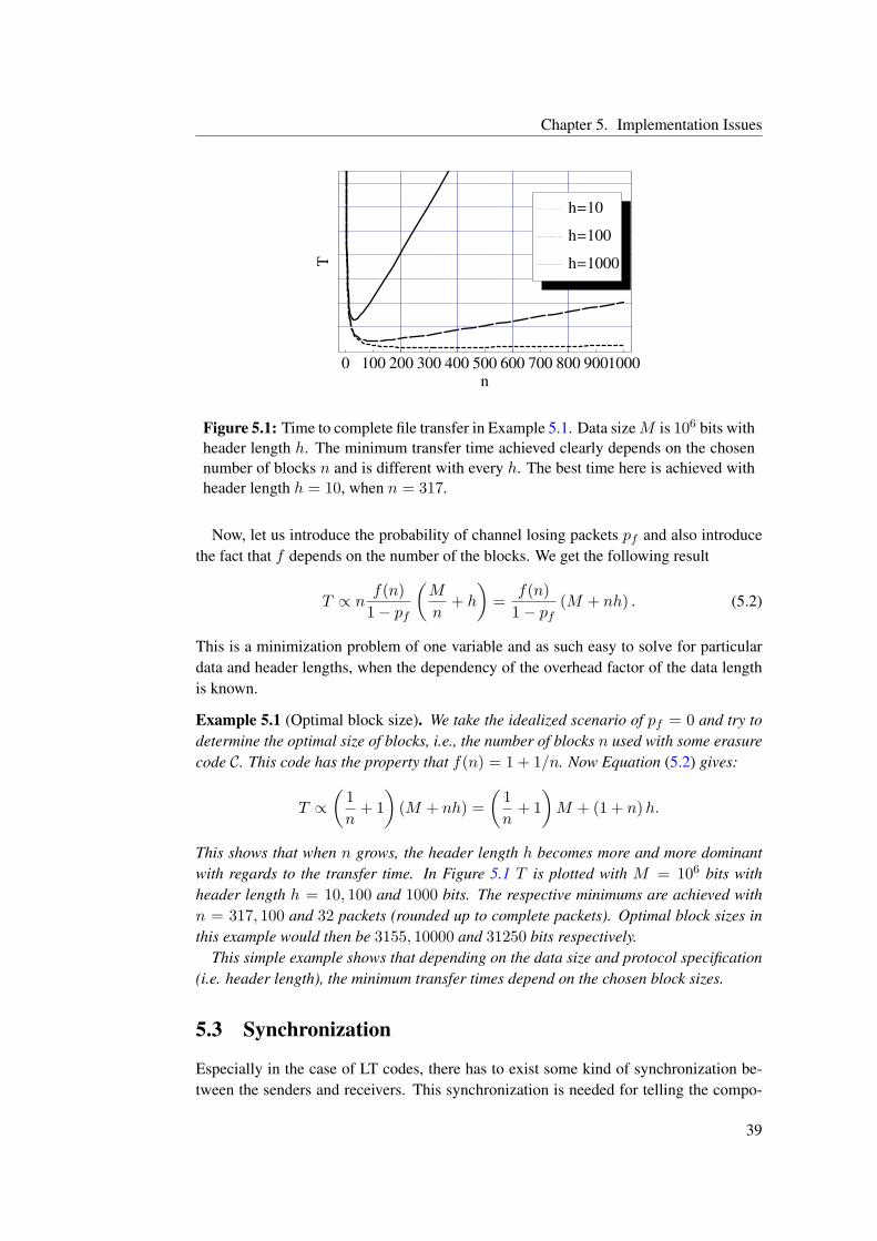
In Chapter 5 we discuss some implementation issues, which need to be addressedwhen doing an actual implementation of any of the presented coding methods. We alsopresent a simple model for calculating the optimal block sizes in this chapter.

Our main contribution is presented in Chapter 6, where we propose an optimizationalgorithm for the degree distribution used in LT code. This chapter presents the derivationof the algorithm with some mathematical background behind it.

Some numerical examples and discussion of the performance of the developed algo-rithm are given in Chapter 7. Finally, Chapter 8 contains the conclusions.

3

Chapter 2

Background in Information Theory

This chapter presents basics in information and coding theory, which are prerequisitesfor understanding the later chapters. Definitions and notation are presented together withsome examples of basic codes. Emphasis is on the concepts which are important andrelevant for this work. Information theory itself is here considered to be an umbrellatheory which contains coding theory as a part. The presentation here is only a scratch ofthe surface on these subjects, a plethora of books have been written on information andcoding theory; references used in this work are [30, 47, 33].

2.1 Transmission of Data

The theme of this thesis is closely connected with efficient transmission of data in acomputer network. Networks represent the information in digital form. This meansthat there is a finite amount of possible symbols used to characterize the information.In computer networks the information is passed trough different kinds of links fromthe source to one or more recipients. These links in information theoretical terms arechannels. Several different channel models exists, some have more theoretical uses butmodels exist also for practical purposes.

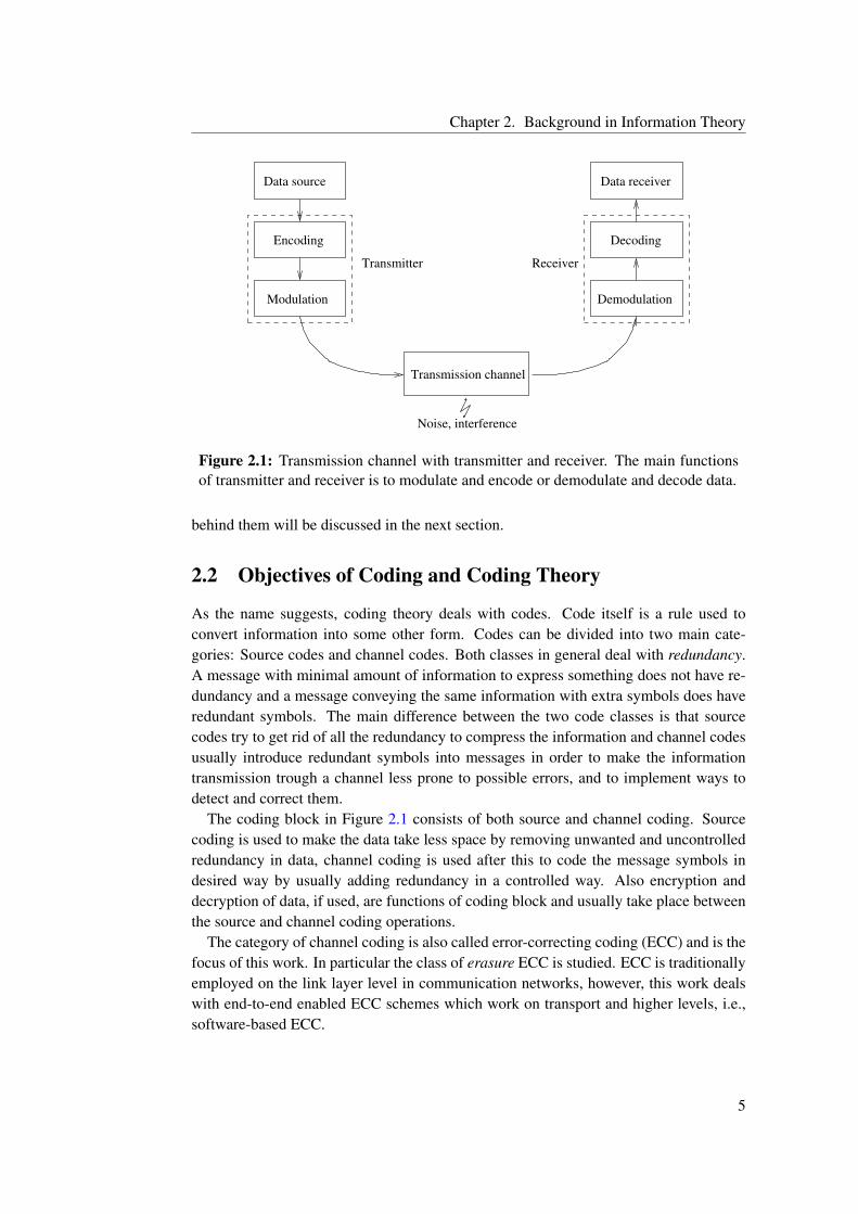
Many, if not all, books on information theory and channel coding related issues havesimilar presentation as Figure 2.1 as the “first picture”. Figure 2.1 shows a basic schemefor information transmission through a channel. The data source generates messages, i.e.,blocks of information to be transmitted to receivers. A generated message ultimately hasan analog or digital signal form and goes trough a transmitter which performs some fun-damental operations on the signal. The two main operations such a transmitter carries outare modulation and encoding. Modulation is used to transform the message to suitableform for a particular transmission channel. This results in an efficient and suitable sig-nal form which hopefully minimizes the interference and noise which the channel mightincur on the signal. The aim is to enable efficient transmission of the signal over thegiven channel type. Modulation is not, however, the subject of this work and for a deepertreatment of modulation issues a good reference is [10].

The coding function performed by the transmitter is more relevant to this work. Cod-ing theory, i.e., the science studying different codes and the mathematical framework

4

Chapter 2. Background in Information Theory

Modulation

Encoding

Demodulation

Decoding

Data receiverData source

ReceiverTransmitter

Transmission channel

Noise, interference

Figure 2.1: Transmission channel with transmitter and receiver. The main functionsof transmitter and receiver is to modulate and encode or demodulate and decode data.

behind them will be discussed in the next section.

2.2 Objectives of Coding and Coding Theory

As the name suggests, coding theory deals with codes. Code itself is a rule used toconvert information into some other form. Codes can be divided into two main cate-gories: Source codes and channel codes. Both classes in general deal with redundancy.A message with minimal amount of information to express something does not have re-dundancy and a message conveying the same information with extra symbols does haveredundant symbols. The main difference between the two code classes is that sourcecodes try to get rid of all the redundancy to compress the information and channel codesusually introduce redundant symbols into messages in order to make the informationtransmission trough a channel less prone to possible errors, and to implement ways todetect and correct them.

The coding block in Figure 2.1 consists of both source and channel coding. Sourcecoding is used to make the data take less space by removing unwanted and uncontrolledredundancy in data, channel coding is used after this to code the message symbols indesired way by usually adding redundancy in a controlled way. Also encryption anddecryption of data, if used, are functions of coding block and usually take place betweenthe source and channel coding operations.

The category of channel coding is also called error-correcting coding (ECC) and is thefocus of this work. In particular the class of erasure ECC is studied. ECC is traditionallyemployed on the link layer level in communication networks, however, this work dealswith end-to-end enabled ECC schemes which work on transport and higher levels, i.e.,software-based ECC.

5


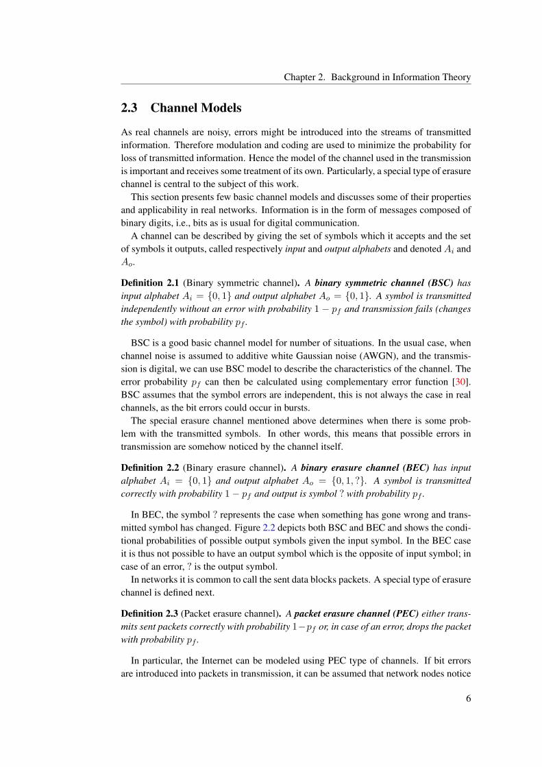
2.3 Channel Models

As real channels are noisy, errors might be introduced into the streams of transmittedinformation. Therefore modulation and coding are used to minimize the probability forloss of transmitted information. Hence the model of the channel used in the transmissionis important and receives some treatment of its own. Particularly, a special type of erasurechannel is central to the subject of this work.

This section presents few basic channel models and discusses some of their propertiesand applicability in real networks. Information is in the form of messages composed ofbinary digits, i.e., bits as is usual for digital communication.

A channel can be described by giving the set of symbols which it accepts and the setof symbols it outputs, called respectively input and output alphabets and denoted Ai andAo.

Definition 2.1 (Binary symmetric channel). A binary symmetric channel (BSC) hasinput alphabet Ai = 0, 1 and output alphabet Ao = 0, 1. A symbol is transmittedindependently without an error with probability 1 − pf and transmission fails (changesthe symbol) with probability pf .

BSC is a good basic channel model for number of situations. In the usual case, whenchannel noise is assumed to additive white Gaussian noise (AWGN), and the transmis-sion is digital, we can use BSC model to describe the characteristics of the channel. Theerror probability pf can then be calculated using complementary error function [30].BSC assumes that the symbol errors are independent, this is not always the case in realchannels, as the bit errors could occur in bursts.

The special erasure channel mentioned above determines when there is some prob-lem with the transmitted symbols. In other words, this means that possible errors intransmission are somehow noticed by the channel itself.

Definition 2.2 (Binary erasure channel). A binary erasure channel (BEC) has inputalphabet Ai = 0, 1 and output alphabet Ao = 0, 1, ?. A symbol is transmittedcorrectly with probability 1− pf and output is symbol ? with probability pf .

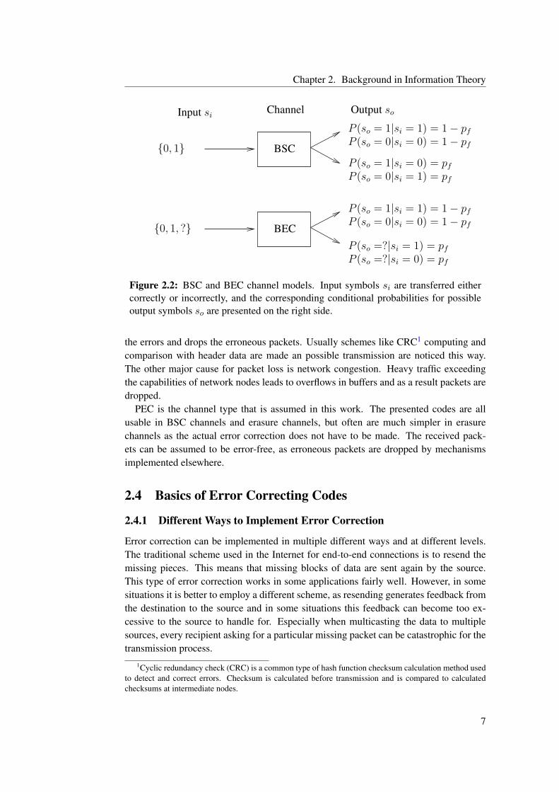
In BEC, the symbol ? represents the case when something has gone wrong and trans-mitted symbol has changed. Figure 2.2 depicts both BSC and BEC and shows the condi-tional probabilities of possible output symbols given the input symbol. In the BEC caseit is thus not possible to have an output symbol which is the opposite of input symbol; incase of an error, ? is the output symbol.

In networks it is common to call the sent data blocks packets. A special type of erasurechannel is defined next.

Definition 2.3 (Packet erasure channel). A packet erasure channel (PEC) either trans-mits sent packets correctly with probability 1−pf or, in case of an error, drops the packetwith probability pf .

In particular, the Internet can be modeled using PEC type of channels. If bit errorsare introduced into packets in transmission, it can be assumed that network nodes notice

6


BSC

BEC

ChannelInput si

0, 1

0, 1, ?

Output so

P (so = 1|si = 1) = 1− pf

P (so = 1|si = 0) = pf

P (so = 0|si = 1) = pf

P (so = 0|si = 0) = 1− pf

P (so = 1|si = 1) = 1− pf

P (so = 0|si = 0) = 1− pf

P (so =?|si = 1) = pf

P (so =?|si = 0) = pf

Figure 2.2: BSC and BEC channel models. Input symbols si are transferred eithercorrectly or incorrectly, and the corresponding conditional probabilities for possibleoutput symbols so are presented on the right side.

the errors and drops the erroneous packets. Usually schemes like CRC1 computing andcomparison with header data are made an possible transmission are noticed this way.The other major cause for packet loss is network congestion. Heavy traffic exceedingthe capabilities of network nodes leads to overflows in buffers and as a result packets aredropped.

PEC is the channel type that is assumed in this work. The presented codes are allusable in BSC channels and erasure channels, but often are much simpler in erasurechannels as the actual error correction does not have to be made. The received pack-ets can be assumed to be error-free, as erroneous packets are dropped by mechanismsimplemented elsewhere.

2.4 Basics of Error Correcting Codes

2.4.1 Different Ways to Implement Error Correction

Error correction can be implemented in multiple different ways and at different levels.The traditional scheme used in the Internet for end-to-end connections is to resend themissing pieces. This means that missing blocks of data are sent again by the source.This type of error correction works in some applications fairly well. However, in somesituations it is better to employ a different scheme, as resending generates feedback fromthe destination to the source and in some situations this feedback can become too ex-cessive to the source to handle for. Especially when multicasting the data to multiplesources, every recipient asking for a particular missing packet can be catastrophic for thetransmission process.

1Cyclic redundancy check (CRC) is a common type of hash function checksum calculation method usedto detect and correct errors. Checksum is calculated before transmission and is compared to calculatedchecksums at intermediate nodes.

7


The previous example is a higher level form of automatic repeat request (ARQ), amethod which is usually employed at link level between two network nodes. In ARQ,the receiver explicitly asks for retransmission of such blocks where errors have beendetected.

Another way to deal with errors is to simply drop the erroneous data and cope withwhat is available. This scheme can be used in some cases when transmitting streamingor analog data, for example in speech transmission. Also in many real-time situations,the data arriving late is completely useless to the recipient. This does not, however,work with digital data transmission, where the transferred information has ultimately totake exactly the same form at both ends of communicating parties. The method of justdropping pieces of information with errors is called muting.

The error control scheme considered further in this work is forward error correction(FEC). In FEC, data is encoded in a way such that based on the erroneous received data,the receiver can use probabilistic analysis to determine what the received data most likelyshould be. FEC can be employed on multiple levels in communications. Traditionally,FEC codes are implemented directly in hardware and thus work at the link layer levelbetween two adjacent network nodes. Software based end-to-end FEC is not yet widelydeployed, but because of the increasing processing capability of desktop computers anddevelopment of efficient codes, the obstacles are not significant anymore. Software FECwould thus be a reasonable choice for some applications [40]. Implementation issues ofsoftware FEC are further discussed in Chapter 5.

2.4.2 Simple Error Correcting Codes

We continue with some useful definitions. The basic model presented if Figure 2.1 in-volves a source who wants to send some information to some receiver.

Definition 2.4 (Message, symbol). Let m denote the message a source wants to transfer.Individual pieces of a message are called symbols. The message can be represented as amessage vector m.

An example of a message vector could be m = (0 0 1), consisting of three sym-bols. These messages are encoded prior to transmission using some code:

Definition 2.5 (Code, codeword). A code is a set of rules for transferring data into an-other form. Equivalently a code is the set C of all legal codewords c. A codeword c isgenerated from the message m with the specified rules. Codewords can be representedby codeword vectors c similarly as messages. Encoding is the process of creating code-words from messages and decoding is the process of transferring codewords back intothe form of the original data.

In particular error-correcting codes are such that they can detect and correct possibleerrors in transmitted data. Perhaps the most common code used to detect errors is calledparity. Parity is a single bit added usually at the end of a codeword indicating whetherthere is an odd or even number of ones in a particular piece of data. Usually parity bit 1means that there is an odd number of ones and 0 is used to indicate even number of ones.

8


Example 2.6 (Parity). We have original message m = (0 0 1) which we want totransfer using parity error-detecting code. Thus the encoder calculates the number ofones in the original message and adds a parity bit accordingly, here the codeword isc = (0 0 1 1). Now if we transfer this codeword over BSC, there is some prob-ability pf independently for every transmitted symbol to change. Now if the receivedcodeword at the receiver side is c = (0 0 0 1), the receiver knows that there hasto be an error somewhere because the number of ones is odd and we are using evenparity. Unfortunately parity code is only an error detecting code and we can neitherknow where the error is nor correct it. Also if there is an even number of bit flips, theparity remains the same and the error cannot even be detected. Thus it is easy to see thatusing only parity is probably not a safe bet. Of course, in situations where pf is verysmall, the probability for two bit flips p2

f is negligible, so in situations the probability forchannel errors is very low and rare errors are not critical, the use of parity only couldbe a sufficient error detecting method.

The simplest form of error-correcting code is repetition code. Here we simply repeatevery sent symbol N times and use a majority vote at the receiver end to decode thetransmitted codeword.

Example 2.7 (Repetition). Let us use the same message m = 001 as before. Usingrepetition with N = 3, the sent codeword is then c = 000000111. If the receiver gets theword c = 001010111, he can assume that first two symbols should be zeros and the lastone should be one. The downside of this scheme is that the length of the sent codewordis three times as long as the original message. A double error in one repeated symbol isdetected but generates a false outcome when majority vote decoding is used. Repetitionis error-correcting code, as it can detect and correct errors.

The parity code has not the ability to correct errors, but is efficient overhead-wise; onlyone symbol is needed in addition to the symbols in original message. Repetition has thedesirable error-correction ability, but every symbol has to be repeated many times. Wedefine the rate of a code as follows:

Definition 2.8 (Rate). When the original message length is n source symbols and it isencoded using a code which produces k encoding symbols, then the rate of the code isR = n

k .

Usually the reciprocal of rate is defined to be the overhead factor f , but we use adifferent definition for the purposes of this work:

Definition 2.9 (Overhead factor). If the original length of a message is n symbols, andthe receiver needs to collect n′ ≥ n encoding symbols (packets) to decode the originalmessage, then the overhead factor is f = n′

n . This definition implies that f ≥ 1.

We will see in the next chapters that it is convenient to separate the overhead causedby encoding redundancy, and the overhead caused by the number of received packets.Depending on the used code, the amount of redundant information transferred mightdepend on the used rate R or on the overhead factor f or on combination of both ofthese.

9


In our parity example, the rate is R = nn+1 = 3

4 , and in repetition example R = 13 ,

which is worse than in parity case. Next we discuss a little bit of the theory behind theerror detection and correction capabilities of codes in general.

Definition 2.10 (Hamming distance). Hamming distance dH of two vectors c1 and c2

is the number of differing symbols of these two messages, i.e,

dH(c1, c2) =∣∣ i | ci

1 6= ci2, 0 < i ≤ k

∣∣ . (2.1)

Minimum Hamming distance dmin of a code C is useful when describing the error detec-tion and correcting capabilities:

dmin(C) = minc1,c2∈C

dH(c1, c2)|c1 6= c2. (2.2)

It can be shown [47] that a code with a minimum Hamming distance dmin can

1. Detect up to l = dmin − 1 errors per codeword.

2. Correct up to t = bdmin−12 c errors per codeword.

With parity code, we see that dmin = 2, as two different valid codewords have to differin two different bits, otherwise the parity would change. Thus we can detect l = 2−1 = 1error in a codeword and correct t = b1/2c = 0 errors as was discussed in Example 2.6.

Only valid codewords in N = 3 repetition code are 000 and 111, the minimum dis-tance is then dmin = 3. Now l = 3 − 1 = 2 errors per codeword can be detected andt = 1 errors corrected, which is in agreement with our discussion in Example 2.7.

2.4.3 Linear Block Codes

We want to have the error correcting capability of repetition codes but with a rate likein the parity codes. A more advanced class of codes than the basic schemes presentedabove are linear block codes. An (n, k) block code is a code where length of data blocksis n symbols and these blocks are encoded to codewords of k symbols. Thus the rate ofsuch a code is R = n/k.

A linear code means that if two codeword vectors are part of the code then also thesum of these vectors belongs to the same code. Also the zero vector belongs to a linearcode. When symbols are bits the summation is performed using modulo-2 arithmetic,i.e., in GF (2), see Appendix A. In general, codeword symbols can be elements of someGF (q).

Linear codes have one useful property: the minimum Hamming distance dmin is thesame as the number of symbols other than zero in a non-zero codeword.

Definition 2.11 (Hamming weight). Hamming weight wH(c) is the number of non-zerosymbols in c.

This means that dH(c, 0) = wH(c) and further for linear codes

dH(c1, c2) = dH(c1 + c2, 0) = wH(c1 + c2), (2.3)

10


where c1 + c2 ∈ C, thusdmin(C) = min

c∈CwH(c). (2.4)

Definition 2.12 (Generator matrix, parity check matrix). A generator matrix G of a codecan be used to calculate codewords:

c = mG, (2.5)

where c is the codeword vector and m the message vector. A parity check matrix H issuch that GHT = 0, this means that for all codewords c ∈ C

cHT = 0. (2.6)

A systematic code is such where the codeword has the original message blocks intact atthe beginning, and redundant information is added at the end of the original information.A systematic form of a linear block code can be constructed by generator matrix

G = (In|P) , (2.7)

where In is a n×n identity matrix and P is a (n)×(k − n) matrix. If G is in systematicform, then the parity check matrix is easy to calculate:

H =(PT| − Ik−n

). (2.8)

Note that if we consider binary codes, then −I = I.

2.4.4 Hamming Codes

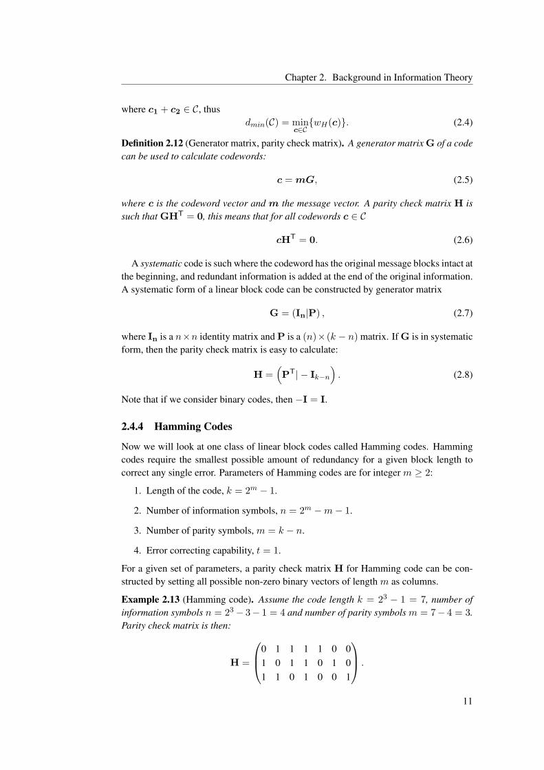
Now we will look at one class of linear block codes called Hamming codes. Hammingcodes require the smallest possible amount of redundancy for a given block length tocorrect any single error. Parameters of Hamming codes are for integer m ≥ 2:

1. Length of the code, k = 2m − 1.

2. Number of information symbols, n = 2m −m− 1.

3. Number of parity symbols, m = k − n.

4. Error correcting capability, t = 1.

For a given set of parameters, a parity check matrix H for Hamming code can be con-structed by setting all possible non-zero binary vectors of length m as columns.

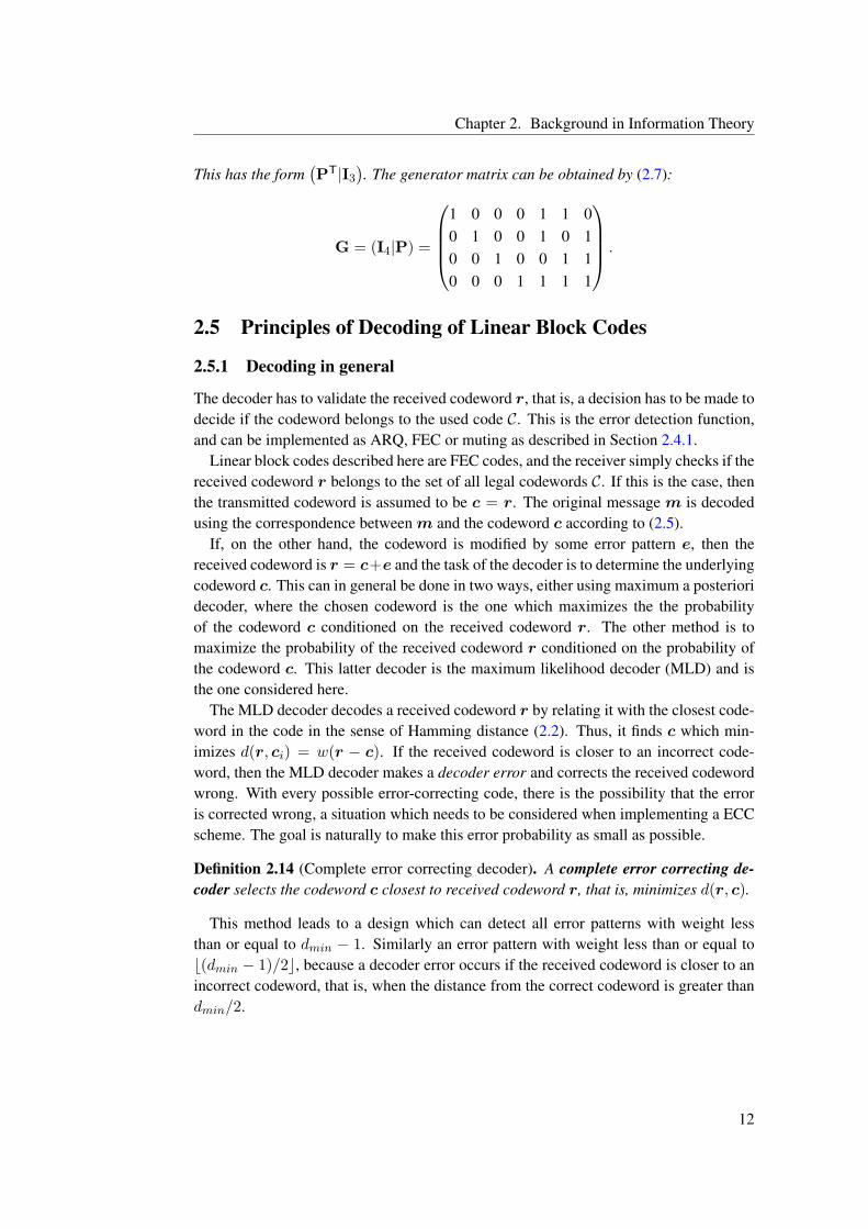
Example 2.13 (Hamming code). Assume the code length k = 23 − 1 = 7, number ofinformation symbols n = 23− 3− 1 = 4 and number of parity symbols m = 7− 4 = 3.Parity check matrix is then:

H =

0 1 1 1 1 0 01 0 1 1 0 1 01 1 0 1 0 0 1

.

11


This has the form(PT|I3

). The generator matrix can be obtained by (2.7):

G = (I4|P) =

1 0 0 0 1 1 00 1 0 0 1 0 10 0 1 0 0 1 10 0 0 1 1 1 1

.

2.5 Principles of Decoding of Linear Block Codes

2.5.1 Decoding in general

The decoder has to validate the received codeword r, that is, a decision has to be made todecide if the codeword belongs to the used code C. This is the error detection function,and can be implemented as ARQ, FEC or muting as described in Section 2.4.1.

Linear block codes described here are FEC codes, and the receiver simply checks if thereceived codeword r belongs to the set of all legal codewords C. If this is the case, thenthe transmitted codeword is assumed to be c = r. The original message m is decodedusing the correspondence between m and the codeword c according to (2.5).

If, on the other hand, the codeword is modified by some error pattern e, then thereceived codeword is r = c+e and the task of the decoder is to determine the underlyingcodeword c. This can in general be done in two ways, either using maximum a posterioridecoder, where the chosen codeword is the one which maximizes the the probabilityof the codeword c conditioned on the received codeword r. The other method is tomaximize the probability of the received codeword r conditioned on the probability ofthe codeword c. This latter decoder is the maximum likelihood decoder (MLD) and isthe one considered here.

The MLD decoder decodes a received codeword r by relating it with the closest code-word in the code in the sense of Hamming distance (2.2). Thus, it finds c which min-imizes d(r, ci) = w(r − c). If the received codeword is closer to an incorrect code-word, then the MLD decoder makes a decoder error and corrects the received codewordwrong. With every possible error-correcting code, there is the possibility that the erroris corrected wrong, a situation which needs to be considered when implementing a ECCscheme. The goal is naturally to make this error probability as small as possible.

Definition 2.14 (Complete error correcting decoder). A complete error correcting de-coder selects the codeword c closest to received codeword r, that is, minimizes d(r, c).

This method leads to a design which can detect all error patterns with weight lessthan or equal to dmin − 1. Similarly an error pattern with weight less than or equal tob(dmin − 1)/2c, because a decoder error occurs if the received codeword is closer to anincorrect codeword, that is, when the distance from the correct codeword is greater thandmin/2.

12


2.5.2 Syndrome Decoding

A general and standard way of decoding linear codes is called syndrome decoding whichconstitutes of calculating a syndrome vector and then decoding the received codewordby a look-up table. The parity check matrix introduced in Definition 2.12 is used here.The property of all legal codewords c satisfying the equation cHT = 0 is the key factorin calculating the syndrome vector s:

s = rHT = (c + e)HT = cHT + eHT = 0 + eHT = eHT.

So the syndrome vector s is function of the error pattern e, and also unambiguous withrespect to different error patterns meaning that different error patterns have differentsyndrome vector.

Using the syndrome vectors we can tabulate all error patterns associated with differ-ent syndrome vectors and use a table look-up to decode received codewords. However,this method is not very scalable as large codes need large tables thus placing memoryrequirements which can be hard to fulfill.

2.6 Shannon Limit for Noisy Channels

There is a trade-off between the decoder error probability and the rate of a code. Usinglower rates lead to design of codes which can correct error patterns with greater weights,as can be seen from the previous discussion on the linear block codes. This would seemto reason that while we lower the rate of some code, the decoder error probability canbe made arbitrary small, and finally, at the limit when the rate goes to zero, the errorprobability also approaches zero.

There is, however, a certain point where the communication succeeds at zero bit errorprobability pb with non-zero rate R. Bit error probability is the average probability thata decoded bit does not match the corresponding message bit. This result was formulatedby information theory pioneer Claude Shannon [43]. The maximum rate we can com-municate over a certain channel with arbitrary small pb is called the capacity C of thechannel.

Theorem 2.15 (Noisy Channel Coding Theorem). For a channel with capacity C thereexists a coding system such that for rates R < C the information can be transmittedwith arbitrary small amount of errors. For R > C it is not possible to transmit theinformation without errors.

This is simple form of this theorem, for complete discussion and proofs, see [30].For the binary symmetric channel the capacity C can be calculated as follows

C(pf ) = 1− pf

[log2

1pf

+ (1− pf )1

1− pf

], (2.9)

where pf is the channel error probability as defined earlier.

13


2.6.1 Optimality of Error Correcting Codes

Shannon’s results prove that reliable codes for different channels exist. The problem is tofind these codes. However, the noisy channel coding theorem can be used to prove thatgood block codes exist for any noisy channel, but the decoding would probably requirea table look-up procedure that is not computionally efficient. The real problem is to findefficient encoding and decoding methods to make it actually worthwhile to use thesecodes.

A code with optimal properties for a given channel would have low encoding anddecoding complexities and a rate that achieves the channel capacity. Different tricksto implement codes with better encoding and decoding complexities exist, including forexample convolutional codes, concatenation of codes, interleaving and so on. Discussionof these and many other code types can be found in any good book on error-correctingcodes or information theory, see e.g. [30].

A particular category of codes which achieve the capacity at the limit, and are alsovery efficient with finite number of message blocks are digital fountain codes, which arepresented in Section 3.3.

The best known codes for Gaussian channels, i.e., AWGN channels with real valuedinput and output, are LDPC codes, which are presented in Section 3.2. These codes canalso be utilized as erasure codes in discrete channels, for example the packet erasurechannel, enabling similar functionality as with digital fountain codes, as we will see inthe next chapter.

14

Chapter 3

FEC codes for erasure channels

In this chapter FEC codes for erasure channels are presented. In this chapter we presentthe basic properties and functions of the codes, a more thorough treatment can be foundin the references. Especially erasure correcting properties are emphasized and error cor-recting details are deliberately left out. First Reed-Solomon codes and Low-DensityParity-Check (LDPC) codes are discussed, and after that the ideas and the inner work-ings of the digital fountain codes are explained, with focus on the LT codes.

3.1 Reed-Solomon codes

Reed-Solomon codes were presented in 1960 [39] and are still widely used in many dif-ferent applications varying from compact discs and other storage devices to computernetworks and space communication. It still is one of the most popular FEC codingschemes. The Reed-Solomon codes are non-binary cyclic linear block codes. Cycliccodes are such where every codeword can be cyclically shifted, and the resulting word isalso a valid codeword. This means that if

c = (c1 c2 . . . cn)

is a codeword in C, then also

c(1) = (cn c1 c2 . . . cn−1)

is a valid codeword of the same code. Reed-Solomon codes are also part of the largeclass of algebraic codes.

With Reed-Solomon codes, we have to fix beforehand the rate, i.e., the amount ofredundant information we are going to use. The rate is always less than one, resulting intransfer of some redundant information. However, the overhead in terms of extra packetsis zero, i.e. f = 1. This is not in general the case with LT and Raptor codes presented inSection 3.3.

15

Chapter 3. FEC codes for erasure channels

3.1.1 Encoding

Several different ways to define Reed-Solomon codes exist. The original definition inReed and Solomon’s work [39] uses evaluation of polynomials over finite fields as thename of the work suggests. Codewords in the Reed-Solomon codes can be produced byconstructing a polynomial of data,

m(x) = m0 + m1x + m2x2 + · · ·+ mn−1x

n−1, (3.1)

where mi denote the source symbols. Instead of binary symbols 0, 1, a finite fieldalgebra and symbols are used for coefficients mi of terms of polynomial c(x), see Ap-pendix A. When (3.1) is evaluated over nonzero elements in GF(2m), codeword c isobtained,

c =(m (1) m (α) m

(α2)

. . .m(α2m−2

)). (3.2)

Other definitions include defining the Reed-Solomon code as a non-binary extension ofBCH codes [33, 47]. To construct a Reed-Solomon capable of correcting up to t errorsthis way we need a generator polynomial which takes the form:

g(x) =b+2t−1∏

i=b

(x− ai

), (3.3)

where b is integer, usually 0 or 1. As Reed-Solomon codes are cyclic codes, all codewordpolynomials can be obtained by multiplying some codeword polynomial c(x) by the gen-erator polynomial g(x). This way using codeword polynomial c(x) another polynomialc(x) is generated c(x) = c(x)g(x). Now using roots αi of generator polynomial (3.3) itfollows,

c(x) is a codeword polynomial⇐⇒ c(αi) = 0, b ≤ i ≤ b + 2t− 1. (3.4)

The following matrix can be constructed using (3.4):

(c0 c1 . . . cn−1)

1 αb

(αb)2

. . .(αb)n−1

1 αb+1(αb+1

)2. . .

(ab+1

)n−1

......

. . ....

1 αb+2t−1(αb+2t−1

)2. . .

(αb+2t−1

)n−1

= 0. (3.5)

The matrix in (3.5) is the parity check matrix H. Matrices of this form are called Van-dermonde matrices [33].

Example 3.1. Let a Galois field GF(8) be generated by primitive element α so that itselements are as presented in Table A.2. To construct a (7, 3) Reed-Solomon code whichcan correct up to t = 2 errors, we can use the following generator polynomial

g(x) = (x− α)(x− α2

) (x− α3

) (x− α4

)= x4 + α3x3 + x2 + αx + α3.

(3.6)

16


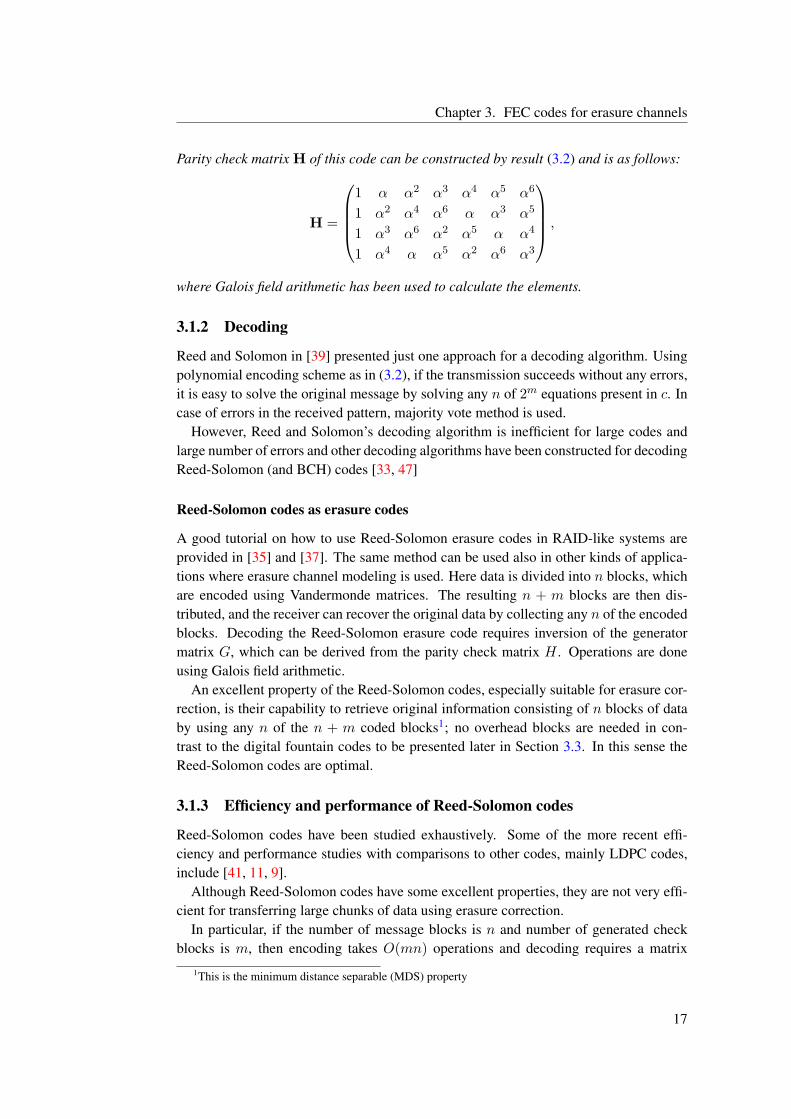
Parity check matrix H of this code can be constructed by result (3.2) and is as follows:

H =

1 α α2 α3 α4 α5 α6

1 α2 α4 α6 α α3 α5

1 α3 α6 α2 α5 α α4

1 α4 α α5 α2 α6 α3

,

where Galois field arithmetic has been used to calculate the elements.

3.1.2 Decoding

Reed and Solomon in [39] presented just one approach for a decoding algorithm. Usingpolynomial encoding scheme as in (3.2), if the transmission succeeds without any errors,it is easy to solve the original message by solving any n of 2m equations present in c. Incase of errors in the received pattern, majority vote method is used.

However, Reed and Solomon’s decoding algorithm is inefficient for large codes andlarge number of errors and other decoding algorithms have been constructed for decodingReed-Solomon (and BCH) codes [33, 47]

Reed-Solomon codes as erasure codes

A good tutorial on how to use Reed-Solomon erasure codes in RAID-like systems areprovided in [35] and [37]. The same method can be used also in other kinds of applica-tions where erasure channel modeling is used. Here data is divided into n blocks, whichare encoded using Vandermonde matrices. The resulting n + m blocks are then dis-tributed, and the receiver can recover the original data by collecting any n of the encodedblocks. Decoding the Reed-Solomon erasure code requires inversion of the generatormatrix G, which can be derived from the parity check matrix H . Operations are doneusing Galois field arithmetic.

An excellent property of the Reed-Solomon codes, especially suitable for erasure cor-rection, is their capability to retrieve original information consisting of n blocks of databy using any n of the n + m coded blocks1; no overhead blocks are needed in con-trast to the digital fountain codes to be presented later in Section 3.3. In this sense theReed-Solomon codes are optimal.

3.1.3 Efficiency and performance of Reed-Solomon codes

Reed-Solomon codes have been studied exhaustively. Some of the more recent effi-ciency and performance studies with comparisons to other codes, mainly LDPC codes,include [41, 11, 9].

Although Reed-Solomon codes have some excellent properties, they are not very effi-cient for transferring large chunks of data using erasure correction.

In particular, if the number of message blocks is n and number of generated checkblocks is m, then encoding takes O(mn) operations and decoding requires a matrix

1This is the minimum distance separable (MDS) property

17


inversion, which is O(n3) operation. As m and n grow, this method becomes sooncomputationally too expensive. Especially when using software to perform the encodingand decoding, computation is demanding due to the arithmetic used which requires extracomputing effort as Galois field arithmetic is not directly supported by typical hardware.Instead look-up tables have to be used for multiplication and addition and this takesextra steps and time in encoding and decoding algorithms. Reed-Solomon codes can beefficiently encoded and decoded using combinatorial logic in digital circuits when thesize of the used Galois field is small, e.g., q ≤ 216.

Recent result of efficient software FEC implementation of Reed-Solomon erasure cod-ing [19] has shown encoding and decoding speeds of 200 Mbps (i.e. 25 MB per second)with a PC with Pentium IV 2.8 Ghz processor, which is a common processor for desktopPC nowadays. This might be sufficient for some applications, but better methods do existas we will soon see.

3.1.4 Specific applications for Reed-Solomon codes

Reed-Solomon codes are widely used in many different technologies. Storage systemsand portable media use Reed-Solomon coding to correct burst errors during data retrievalor playback. Applications in telecommunications include wireless technologies, digi-tal subscriber lines and satellite communications. Also NASA has used Reed-Solomonbased codes in their space missions.

3.2 Low-Density Parity-Check codes

Low-Density Parity-Check (LDPC), also called Gallager codes after their inventor, werepresented in 1960 [14, 15]. These codes were largely forgotten for over forty years,largely due to the fact that computing power has been expensive and inadequate duringthe past decades for efficient use of LDPC codes and other codes have been thought tobe better alternatives. Nowadays LDPC codes can be regarded as an viable alternativeto Reed-Solomon erasure codes in different applications [38]. Since the “rediscovery”of LDPC codes in the 1990s, theoretical analysis of different LDPC coding methods hasbecome popular but the practical side could get more attention.

3.2.1 Encoding of LDPC code

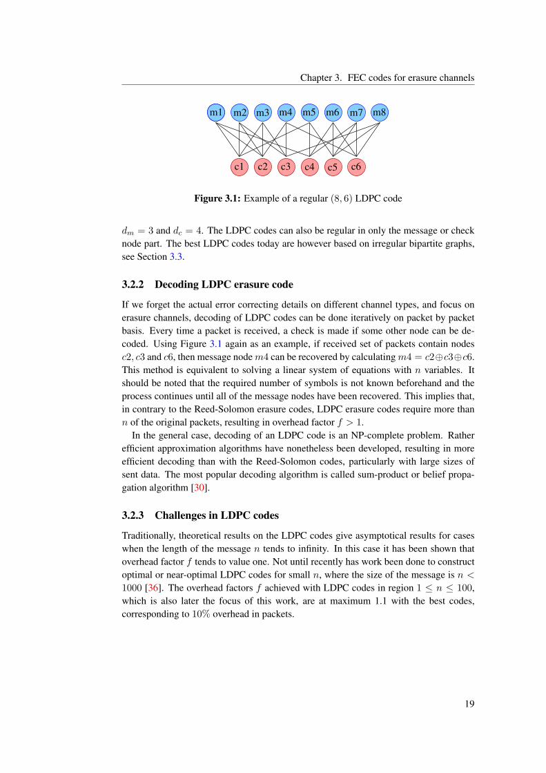
LDPC encoding procedure can be depicted using bipartite graphs, which determine howthe parity symbols are generated from the original message. The n nodes representingmessage bits are called message nodes and k − n nodes representing parity symbols arecalled check nodes. An example of a LDPC code defined using a bipartite matrix ispresented in Figure 3.1. Calculation of check nodes can be read directly from the graph:Check node c2 = m1 ⊕m2 ⊕m3 ⊕m4, where ⊕ denotes the exclusive-or operation,which operates the same way as addition in GF(2), see Appendix A. Both message nodesand check nodes are sent to recipient, the sent symbols are called packets in this context.

A regular LDPC code has the same degree dm in all message nodes and similarly thesame degree dc in all check nodes. The graph in Figure 3.1 is regular in both parts, where

18


m1 m2 m3 m4 m5 m6 m7 m8

c6c5c4c3c2c1

Figure 3.1: Example of a regular (8, 6) LDPC code

dm = 3 and dc = 4. The LDPC codes can also be regular in only the message or checknode part. The best LDPC codes today are however based on irregular bipartite graphs,see Section 3.3.

3.2.2 Decoding LDPC erasure code

If we forget the actual error correcting details on different channel types, and focus onerasure channels, decoding of LDPC codes can be done iteratively on packet by packetbasis. Every time a packet is received, a check is made if some other node can be de-coded. Using Figure 3.1 again as an example, if received set of packets contain nodesc2, c3 and c6, then message node m4 can be recovered by calculating m4 = c2⊕c3⊕c6.This method is equivalent to solving a linear system of equations with n variables. Itshould be noted that the required number of symbols is not known beforehand and theprocess continues until all of the message nodes have been recovered. This implies that,in contrary to the Reed-Solomon erasure codes, LDPC erasure codes require more thann of the original packets, resulting in overhead factor f > 1.

In the general case, decoding of an LDPC code is an NP-complete problem. Ratherefficient approximation algorithms have nonetheless been developed, resulting in moreefficient decoding than with the Reed-Solomon codes, particularly with large sizes ofsent data. The most popular decoding algorithm is called sum-product or belief propa-gation algorithm [30].

3.2.3 Challenges in LDPC codes

Traditionally, theoretical results on the LDPC codes give asymptotical results for caseswhen the length of the message n tends to infinity. In this case it has been shown thatoverhead factor f tends to value one. Not until recently has work been done to constructoptimal or near-optimal LDPC codes for small n, where the size of the message is n <

1000 [36]. The overhead factors f achieved with LDPC codes in region 1 ≤ n ≤ 100,which is also later the focus of this work, are at maximum 1.1 with the best codes,corresponding to 10% overhead in packets.

19


3.3 Digital fountain codes

This section presents the work done by Michael Luby et al. They have made improve-ments based on the LDPC codes and presented very good codes under their digital foun-tain content distribution system. They have also founded a company Digital FountainInc. [2], whose business is to develop and license technology based on their efficientFEC erasure codes. Tornado, LT and Raptor codes are presented next, LT codes get thedeepest treatment as they are the main topic of this work.

3.3.1 Background

In [30] a few methods are presented to make the LDPC codes to work more efficiently.One method is to use Galois fields or similar constructs to clump bits together. Anothermethod to improve the performance is to make the graph irregular. This is discussedin [28] and also further demonstrated that irregular graphs outperform regular graphs inLDPC coding. Irregularity of the graphs is the vital reason for digital fountain codes tobe so efficient and successful in erasure correction.

This idea was taken further by Luby et al. and new class of codes, called Tornadocodes, was developed in 1997 [29, 9]. These were the first kind of codes to efficientlyapproximate a digital fountain. What Luby et al. call a digital fountain is an idealizedmodel of content distribution: A source generates potentially an infinite amount of en-coded packets and sends those into a network. The recipients of data need to collect onlya certain amount of these packets to decode the original data. The term digital fountaincomes from an analogy to a fountain: Server in this case is the fountain, who sprayspackets corresponding to water drops, and recipients are analogous to buckets which isused to collect water. When the bucket is full, the process is finished and it does notmatter which specific water drops were collected. Similar situation exists with the digi-tal fountain concept: packets are received and it does not matter which specific packetsare received. In ideal situation, if the original data consists of n encoded packets, onlyn packets need to be collected by the recipients. This can be achieved using codes withthe MDS property, e.g., the Reed-Solomon codes presented earlier in Section 3.1. How-ever, as discussed, computational complexity of the Reed-Solomon codes makes themimpractical for use in case of large amount of data and block length. Thus Luby et al.have developed other kinds of codes for approximating the digital fountain.

3.3.2 Tornado codes

First class of codes published under the digital fountain concept, Tornado codes, workmuch more efficiently than Reed-Solomon codes in erasure correcting. In [9] the per-formance of Tornado codes is directly compared to Reed-Solomon codes. The presentedresults show that the Tornado codes are a much better alternative to approximating thedigital fountain than the Reed-Solomon codes.

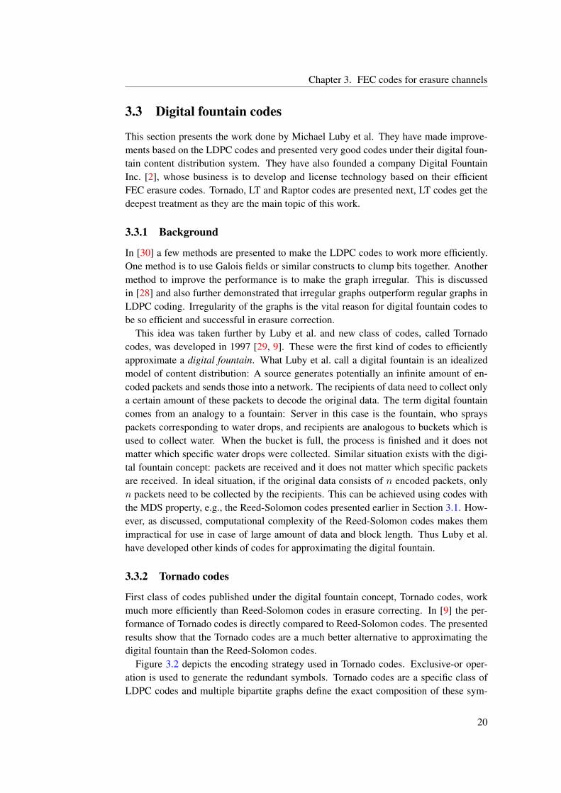
Figure 3.2 depicts the encoding strategy used in Tornado codes. Exclusive-or oper-ation is used to generate the redundant symbols. Tornado codes are a specific class ofLDPC codes and multiple bipartite graphs define the exact composition of these sym-

20


bols. Rate of the used Tornado code has to be fixed in advance, similarly as with Reed-Solomon codes. The composition of the bipartite graphs has to be be well though out inorder to enable efficient encoding and decoding and to provide erasure correcting caba-bilities. A detailed discussion of good bipartite graphs for this purpose is given in [29].

If the number of the blocks the message is divided into is n, the recipient needs tocollect a little more than n of the encoded packets in order to decode the original message(i.e., fn packets needs to be collected). This erasure correcting property enables theTornado codes to approximate the digital fountain. The trade off compared to Reed-Solomon codes is this number of extra packets needed for decoding, but a good codedesign results in much better overall performance. The overhead factor f of Tornadocodes can be tuned to around f ≈ 1.05 for large n and k, an example is given in [29]. Theencoding and decoding times of Tornado codes are proportional to k log 1/(f − 1)M ,where M is the size of the original message.

XOR

XOR

k−n redundant symbolsnoriginalmessagesymbols

Figure 3.2: Idea of the Tornado codes. The k − n redundant symbols are generatedby exclusive-or operation in the way the bipartite graphs define. In order to decode theoriginal message, the recipient has to collect a little more than n packets.

Although the Tornado codes are better in approximating the digital fountain than theReed-Solomon codes, they are not ideal. The rate has to be fixed beforehand, and withtoo large a rate, it turns out that the recipient receives duplicate packets, which are uselessand deteriorate the channel efficiency. Conversely, if the rate is small, then memory andencoding requirements make the Tornado codes perform poorly. Luckily, better codesfor the digital fountain scheme exist, as we will see next.

3.3.3 LT codes

LT codes were published by Michael Luby in a landmark paper in 2002 [27]. These codesare rateless, meaning that the rate does not need to be fixed beforehand, and encodingsymbols can be generated on the fly. LT codes are also first class of codes which are a

21


full realization of the digital fountain concept presented in [9].

Encoding of LT code

The encoding process is surprisingly simple. Following the tradition of LDPC codespresented earlier, also LT codes can be defined using a bipartite graph. This graph isirregular in LT codes, and a degree distribution is used to determine the degrees of en-coding symbols.

Definition 3.2 (Degree distribution, generator polynomial). The degree distribution ρ(d)of LT code is a probability distribution, where ρ(i) is the probability of generating anoutput symbol consisting of i input symbols. Degree distribution can also be presentedas a generator polynomial Ω(x) =

∑ki=1 Ωix

i, where Ωi is the probability for choosingvalue i.

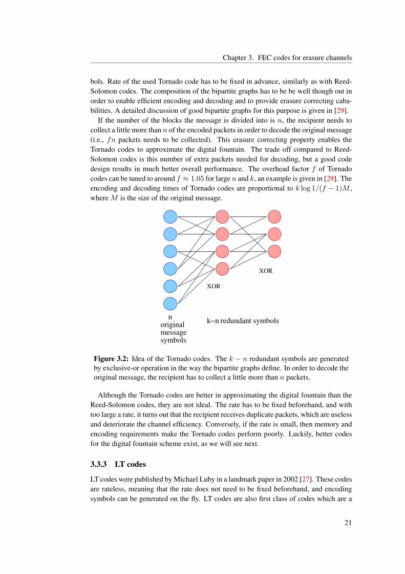
Degree distribution is sampled to obtain value d, which is used as the degree for out-put symbol c(i) in the encoding graph. Output symbol is generated by choosing d in-put symbols m(i) uniformly at random and calculating sum of these symbols in GF(2)arithmetic. This is illustrated in Figure 3.3. Also listing Algorithm 3.1 shows the generalframework of an encoding algorithm for the LT code. Stopping condition for the encod-ing algorithm could be specified by the number of output symbols agreed beforehand orwhen the recipient has enough symbols to decode the original message.

It should be noted that it does not matter what the symbol length is. One input symbolcould be just one bit or a vector of bits, the encoding and decoding processes are thesame regardless and the XOR operation is done bitwise to the whole vector.

Algorithm 3.1 A general LT encoding algorithm1: procedure LTENCODE

2: repeat3: choose a degree d from degree distribution ρ(d).4: choose uniformly at random d input nodes m (i1) , . . . ,m (id).5: c(i)← m (i1)⊕m (i2)⊕ · · · ⊕m (id).6: until enough output symbols are sent7: end procedure

Decoding of LT codes

Decoding is done similarly as decoding of the LDPC erasure codes. The decoding pro-cedure needs the information of degree values of each encoding symbol it receives andthe information of which source symbols are added together in a output symbol.

This information needs to be included somehow in the encoding procedure, furtherdiscussion of this topic follows in Chapter 5.

Decoding is started by receiving a degree-one output symbol. This symbol clearly hasto be the same as the input symbol which it copied in the encoding process. This way, wehave one input symbol uncovered, i.e., its value is known. Next we add this value (using

22


Input symbols

Choose d symbols

XOR

Output symbol

Figure 3.3: LT encoding. Value d is sampled from a degree distribution, output symbolis generated by successively using XOR to d selected input symbols

exclusive-or) to all neighbors of this uncovered symbol and remove the edges in thedefining graph between the uncovered input symbol and its neighbors thus decreasingdegrees in all of the neighboring output symbols. This way we have possibly moredegree-one output symbols and the process may continue. An example illustration of thedecoding process is presented in Figure 3.3.3. A framework of an decoding algorithm issketched in listing Algorithm 3.2.

It should be noted that decoding LT code in this way is suboptimal in the sense that allof the information of the received packets is not used. For example, if source messageconsists of n = 3 blocks, the recipient could decode the original message if he hadthree different packets which each consists of two symbols. This, however, would makethe decoding algorithm computationally too intense, as this method equates to solving alinear system of equations, an operation which is in general case too inefficient for thisproblem.

Algorithm 3.2 A general LT decoding algorithm1: procedure LTDECODE

2: repeat3: repeat4: receive a packet5: until degree one check node cn is available6: mk ← cn . message node mk has to be same as cn

7: calculate ci = mk ⊕ ci for all ci connected to mk

8: remove all edges between mk and check nodes9: until original message is fully recovered

10: end procedure

Degree distributions

As stated earlier, the degree distribution plays an extremely important role in the LTcoding process. Without a proper distribution, the whole concept of LT codes would be

23


Figure 3.4: Illustration of decoding LT code. From top left to bottom right: Theencoding procedure defines a bipartite graph, where each output symbol has one ormany input symbols as neighbors. First we look for degree one (one neighbor) outputsymbol; we have one, so we know that the middle input symbol is 0. Now we canremove the edge between lower and upper parts. Next we XOR 0 with every connectedoutput symbol, we have only one connection and XOR for 0 with 1 is 1. After this weremove the edge between operated 0 and 1 nodes. Now we look again for degreeone symbols. There exists one such node, so again we remove the edge, and XORthe corresponding input symbol with all connected output symbols. Now the twoconnected output symbols change to 0. Next we remove the edges and in final step wehave two degree one nodes which uncover the last unknown input symbol.

24


rather useless. The remarkable result proved by Luby in [27] is that efficient distributionsdo exist for LT codes.

As the degree distribution is the only factor which defines the efficiency of LT coding,the following two general principles can be stated about the design of a good degreedistribution:

1. The number of output symbols which ensures the decoding of the original messageshould be as low as possible to keep the overhead factor f low.

2. The average degree of the output symbols should be as low as possible, so thenumber of steps needed in the decoding algorithm stays as low as possible.

The LT decoding process needs degree one symbols to keep the decoding going on.The ripple in LT process is the amount of input symbols which have been uncoveredbut not yet processed, i.e., number of input symbols in state of line 6 in Algorithm 3.1.The symbols in the ripple are then processed one by one as the rest of the algorithmstates, possibly growing or decreasing the ripple as new input symbols are covered bythe process.

Optimally the ripple is one in each step, thus one symbol can be used to decode oneinput symbol and further remove edges from the encoding graph. If number of availabledegree one symbols is larger than one, the received symbols are redundant thus increasingthe inefficiency through a larger overhead factor f . On the other hand ripple should notgo to zero at any point of the decoding process, otherwise the decoding halts and isunsuccessful. Consequently, the size of the ripple should be kept above one to avoid thecomplete disappearance of the ripple.

Let us denote n(t)i the number of output nodes of degree i at time t. Time instant t = 0

corresponds to the start of the decoding algorithm, when the first degree one packet isavailable but none of the original blocks is yet decoded. Thus in the beginning, nodes ofdegree i have i · n(0)

i edges in total connecting to the input nodes. This means that onaverage, one input node has i · n(0)

i /N neighbors of degree i. For clarity we denote thenumber of input nodes here by capital N instead of the lowercase n used elsewhere inthis work. For example, in Figure 3.3.3 at the first phase in top left, the average number ofoutput symbols of degree two as neighbors of input symbols is (2 ·3)/3 = 2. Now, whenan output symbol of degree one is processed and the edges removed accordingly, thenumber of degree i packets whose degree decrease by one is in expectation the averagei · n(0)

i /N . If already t (i.e., at time t) input symbols have been decoded, the edges haveonly n− t input nodes to connect to, so the average is i · n(t)

i /(N − t).The optimal condition in terms of notation presented above, is

n(t)1 = 1 ∀ t ∈ 0, . . . , N − 1. (3.7)

The optimal distribution can be now constructed by considering which conditions leadto the optimal situation in each step as presented above, i.e., what are the values of n

(0)i

for different degrees i. Naturally from (3.7) we have n(0)1 = 1. Value of n

(0)2 has to be

such that at time t = 1 the amount of degree one nodes is again one, this means that one

25


of the degree two nodes at time t = 0 decreases its degree, so we have the equation

2 · n(0)2

N= 1 ⇐⇒ n

(0)2 =

N

2, (3.8)

and more generally at time t

2 · n(t)2

N − t= 1 ⇐⇒ n

(t)2 =

N − t

2. (3.9)

By continuing this reasoning recursively one obtains the rest of the values n(0)i . The

number of degree two nodes at time t is the same as number of degree two nodes attime t − 1 minus the nodes which optimally decrease their degree plus the nodes whichpreviously were of degree three, i.e.,

n(t+1)2 = n

(t)2 −

2 · n(t)2

N − t+

3 · n(t)3

N − t

N − t− 12

=N − t

2− 1 +

3 · n(t)3

N − t

∣∣∣∣−N − t

2

−12

= −1 +3 · n(t)

3

N − t

⇒ n(t)3 =

N − t

2 · 3(3.10)

Hence, the value we are looking for, n(0)3 = N/(2 · 3). The general state equation for

degree i nodes at time t is

n(t+1)i = n

(t)i −

i

N − tn

(t)i +

i + 1N − t

n(t)i+1, (3.11)

which can be solved for n(t)i+1:

n(t)i+1 =

N − t

i + 1

(n

(t+1)i − n

(t)i

)+

i

i + 1n

(t)i . (3.12)

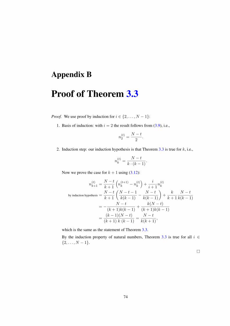
Equation (3.12) gives recursively the rest of the values. The next theorem, however,provides a simpler form.

Theorem 3.3. The number of degree i nodes at time t leading to optimal degree distri-bution in expectation, i.e., provides ripple of one in expectation is

n(t)i =

N − t

i(i− 1). (3.13)

Proof. Proof follows from the discussion above and from Equation (3.12) with induction.Details of the proof by induction are given in Appendix B.

26


Now, the actual values we are looking for are n(0)i . By Theorem 3.3 these are

n(0)i =

N

i(i− 1)for i ∈ 2, . . . , N − 1, (3.14)

and n(0)1 = 1. In order to get the needed probability distribution, we divide these optimal

numbers of different degree nodes at time 0 by the total number of blocks in the message,i.e., we normalize the values n

(0)i in order to get a probability distribution. We arrive at:

Definition 3.4 (Ideal Soliton distribution). The Ideal Soliton distribution ρ(i) is:

ρ(i) =

1n when i = 1

1i(i−1) for i = 2, . . . , n.

Beginning of this distribution is presented in Figure 3.5 for n = 1000. As the basis forconstructing this distribution was ideal behavior in expectation, it is not surprising thatin practice the Ideal Soliton distribution does not work well. The expected ripple size ofone will vanish with variance, resulting in poor performance.

5 10 15 20 25d

0.1

0.2

0.3

0.4

0.5

p@dD

Figure 3.5: Start of the Ideal Soliton distribution for n = 1000

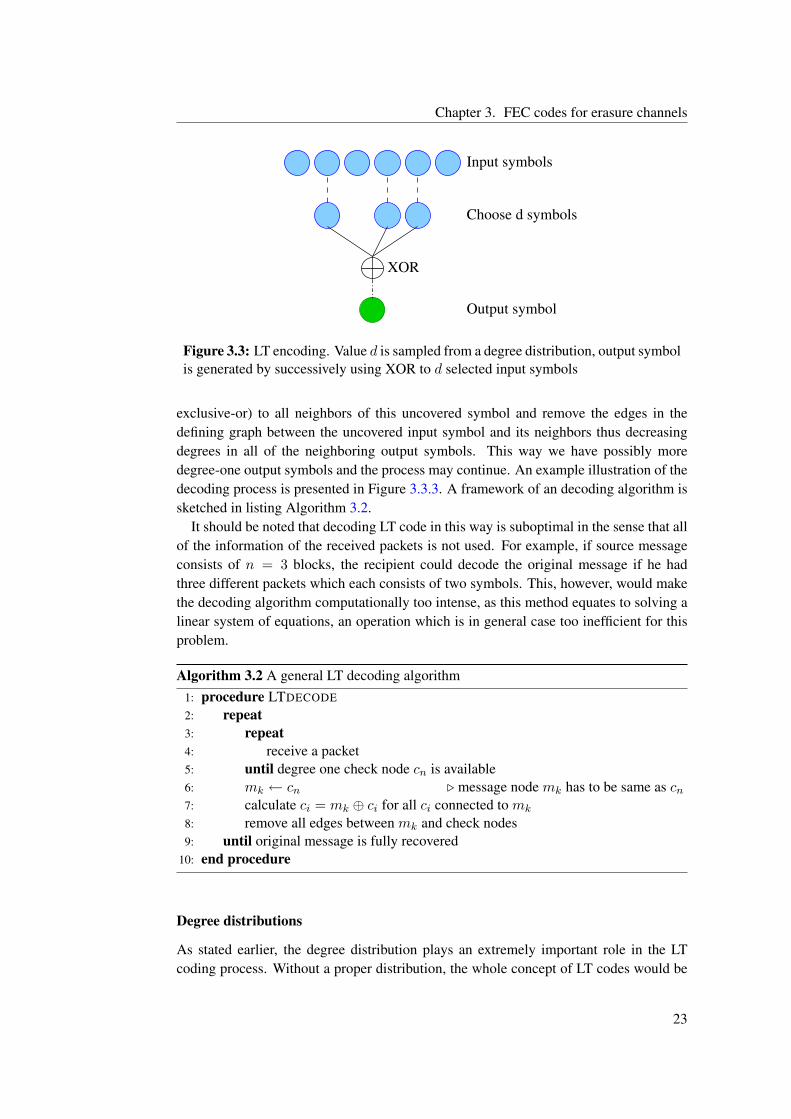
The main results in Luby’s work [27] concern the Robust Soliton distribution, whichis an advanced version of the Ideal Soliton distribution. The goal is to keep the ripple solarge that it will not vanish at any point of the decoding process and also to minimize theexpected ripple size so that the redundancy is kept low.

Definition 3.5 (Robust Soliton distribution). For the Robust Soliton distribution, firstdefine the function:

τ(i) =

Rin for i = 1, . . . , n

R − 1R log R/δ

n for i = nR

0 for i = nR + 1, . . . , n,

27


where δ is the failure probability of decoding process after n′ encoded symbols andR = c · log (n/δ)

√n for some constant c > 0. The Robust Soliton distribution µ(i) is

the normalized value of the sum ρ(i) + τ(i):

µ(i) =ρ(i) + τ(i)∑ni=1 ρ(i) + τ(i)

.

An example of the Robust Soliton distribution with parameters δ = 0.95 and c = 0.2for n = 1000 is presented in Figure 3.6. In short, the addition of τ(i) in Definition 3.5should ensure that:

1. The process starts with large enough ripple.

2. The ripple decrease of one every time a input symbol is uncovered is countered byincreasing the ripple by one.

3. All input symbols are covered at the end of the process by placing spike τ(n/R)at some high degree.

The Robust Soliton distribution was used in [27] to proof that original message canbe recovered from n + O(

√n log2(n/δ)) output symbols with probability 1 − δ. The

encoding and decoding complexities are then O(log(k/δ)) in terms of arithmetic opera-tions.

5 10 15 20 25d

0.1

0.2

0.3

0.4

0.5

0.6

p@dD

Figure 3.6: Start of the Robust Soliton distribution for n = 1000. Parameters areδ = 0.95, c = 0.2. Note the spike at n = 23.

Linear Systems of Equations Approach to LT Codes

As stated above, the LT codes could also be described with the help of linear systemsof equations. The encoded symbols used in LT codes are actually linear equations of n

possible variables, as seen in for example the description of Algorithm 3.1. The degree

28


distribution gives a random value which is used to choose d blocks from the originalmessage, which are then combined using XOR, which equals to modulo-2 addition.

This approach leads to very low overheads, which is also rather easy to calculate an-alytically. To decode the message by solving a linear system, i.e., by matrix inversion,we need to have exactly n linearly independent equations. In other words, if we wantto decode the original message in exactly n steps, we need a n × n matrix of full rank.Let us first calculate the probability of generating a random n × n full rank matrix. Weconsider the generation on row-by-row basis, where each block is chosen to be includedwith probability 1/2. This means that there are 2n possible choices for one row. Theall zeros vector is not accepted, as it is linearly dependent with all other vectors, andcorresponds to a message with no information. So, at the first step we have 2n− 1 possi-bilities to choose from, i.e., the probability to succeed (generate one linearly independentvector) is (2n−1)/2n. To generate a new linearly independent vector, we exclude the allzero vector and the one generated before, i.e., the probability is now (2n − 2)/2n. Thirdvector has to be different from the zero vector and all vectors generated before. Also thelinear combination of two previously generated vectors is not accepted now. The numberof linearly dependent vectors that can be generated from i vectors is:(

i

0

)+(

i

1

)+(

i

2

)+ · · ·+

(i

i

)= 2i, (3.15)

where each binomial term(

ik

)represents the number of linearly dependent vectors that

can be formed by choosing any k equations from the i possible ones. The second term(i1

)corresponds to any previously generated equation and the special case of zero vector

is handled by the first term,(

i0

)= 1.

This means that after i−1 linearly independent equations, the probability of generatingthe ith linearly independent random equation is

2n − 2i−1

2n= 1− 2i−1−n, (3.16)

where the subtracted term in the numerator corresponds to the number of linearly depen-dent vectors that can be generated from i−1 previous linearly independent vectors. Thisleads us to the probability for successionally generating n linearly independent vectors:

Pn =n∏

i=1

(1− 2i−1−n

). (3.17)

The probabilities for n = 1 . . . 20 are plotted in Figure 3.7. As n tends to infinity, theprobability converges approximately to 0.2888, hence the probability of generating a fullrank n× n random matrix is about 29%.

What if the generation does not succeed in n steps? If the generated n equationsinclude n− 1 linearly independent ones, then the we can calculate the probability for thenew equation to be linearly independent of the rest with (3.16):

1− 2n−1−n = 1− 2−1 =12

(3.18)

29


2 4 6 8 10 12 14 16 18 20n

0.3

0.35

0.4

0.45

0.5

Pro

babi

lity

Figure 3.7: Probability that n random generated binary n-vectors with probabilityp = 1/2 are all linearly independent. The probability converges to 0.2888.

Thus, the probability of not succeeding in n steps, but requiring n + n′ steps decreasesroughly like 2−n′

.To calculate the expected number of random equations needed for full rank, we note

that the probability that we need i additional packets to generate the next linearly inde-pendent equation is geometrically distributed:

Qi = (1− p)pi−1, i = 1, 2, . . . (3.19)

where p is the probability that we fail to generate next linearly independent equation.The expectation of (3.19) is:

∞∑i=1

iQi = (1− p)∞∑i=1

ipi−1 = (1− p)1p

∞∑i=1

ipi =1− p

p

∞∑i=1

pd

dppi

= (1− p)d

dp

∞∑i=1

pi = (1− p)d

dp

p

1− p

= (1− p)(1− p)− p(−1)

(1− p)2=

11− p

. (3.20)

We therefore define the number of extra equations needed for a full rank random matrix,when we already have k linearly independent equations, to be

rk =1

1− pk, (3.21)

where the probability of failure in the next step pk = 2k−1/2n = 2k−1−n (compareto (3.16)). Now the following sum gives the total expected number of random equationsneeded for a random full rank n× n matrix:

n∑k=1

rk =n∑

k=1

11− pk

=n∑

k=1

11− 2k−1−n

. (3.22)

In Figure 3.8 we have plotted the expected number of overhead equations, i.e.,∑

rk−k,

30


2 4 6 8 10 12 14 16 18 20n

1

1.1

1.2

1.3

1.4

1.5

1.6

Ove

rhea

din

equa

tions

Figure 3.8: The expected number of overhead equations to generate a random fullrank n× n matrix.

for k = 1, . . . 20. We see that the overhead seems to converge to 1.6 equations forlarge n, for example when n = 1000 the overhead is 1.61 equations. Thus the overheadin general with this approach would be under 2 packets regardless of the value of n.However, decoding of a code generated in this way requires the solving of a full systemof linear equations, which generally is an inefficient operation.

Note that this same approach can also be taken with LDPC codes, where of course thegeneration of the equations is different, depending on the parity check matrix H.

3.3.4 Raptor codes

Raptor codes were developed by Amin Shokrollahi while he was working at DigitalFountain. The discussion provided here is adapted from a preprint paper [44]. Raptorcodes are an essential part of Digital Fountains current content delivery system and wererecently chosen as part of 3GPP’s2 Multimedia Broadcast/Multicast Service (MBMS)for 3rd generation cellular networks.

Encoding and decoding complexities of Raptor codes are linear, and thus efficiency isbetter than with LT codes, where the decoding cost in average per symbol is O(log(n)),resulting in at least O(n log(n)) total cost [44]. This is achieved by relaxing the re-quirement that all input symbols needs to be recovered. Raptor codes are defined as anextension to LT codes: original message m(x) is passed trough a preliminary codingprocess called pre-coding, producing intermediate nodes and these intermediate nodesare passed to LT encoder as input nodes. The code used for pre-coding is denoted C.This process is visualized in Figure 3.9. When defined this way, we see that first class ofRaptor codes are LT codes without pre-coding. Pre-coding can also be done in severalsteps, e.g., first use a basic Hamming code to encode the message and encode outputsymbols of the Hamming code using an LDPC erasure code to produce the intermediatesymbols for LT encoder. Also codes without LT coding can be regarded as a subclass of

23GPP (3rd Generation Partnership Project) is a collaboration agreement between a number of telecom-munications standards bodies (Organizational Partners). Also telecommunications industry has its ownMarket Representation Partners. 3GPP’s scope is to produce specifications and reports for 3G mo-bile system based on GSM and to maintain and develop GSM specifications and reports. See http://www.3gpp.org.

31

http://www.3gpp.org

http://www.3gpp.org


Raptor codes, called pre-coding-only or PCO Raptor codes.By using some erasure correcting code as the precode, the requirement to recover all

input symbols of the LT code is lifted: only a constant fraction of LT encoded symbolsneeds to be recovered, the original message can then recovered by the erasure correctingproperty of the code used for pre-coding.

LT−codingmessage nodes for

Precoding

LT−coding

LT−code check nodes

original message nodes

Figure 3.9: Example of Raptor coding. Original message is encoded using some tra-ditional erasure correcting code, e.g. LDPC code. This process produces intermediatenodes, shown in the middle row, and these are encoded using LT code to produce theoutput symbols.

The decoding of Raptor code is done by first using the LT decoding process to producethe intermediate code and after that input nodes are recovered by applying decodingalgorithm for code C.

32

Chapter 4

Applications

This chapter presents some of the possible applications for the state-of-the-art codingschemes presented in this work. Traditionally erasure and FEC coding are employed insituations where channel errors are abundant, the applications proposed in this chaptercould work efficiently even if the error rate is reasonable. All of the presented applica-tions are some form of content distribution or data storage systems and usually deal withlarge data files.

4.1 Reliable Multicast

Multicast means information delivery at the same time to many different receivers, incontrast to point-to-point delivery or unicast. In computer networking, different kind ofmulticast schemes have been developed using various techniques, at different levels orlayers and for different purposes. In the first descriptions of the fountain coding principle,the particular application considered was multicasting large chunks of data to multiplerecipients from one source (server) [8].

Often multicast refers to IP multicast, where data is sent to a multicast IP address,corresponding to a group of recipients (multicast group). IP multicast is by no meansa simple process, multiple algorithms and protocols take part in a successful multicasttransfer. The major problem with IP multicast, compared to other protocols enablingsimilar function, lies in the history of the TCP/IP protocol stack. In particular, the orig-inal usage of IP protocol did not take into account multicast scenarios and the currentfunctionality is acquired through extensions. The IP protocol provides only best-effortnetwork, and the state information which needs to be stored when using multicast doesnot fit into the best-effort principle. Composition and location of nodes participating ina multicast group has to be stored in the intermediate nodes, and the packets have tobe routed to the specific locations of the receivers. This leads to high inefficiencies andcomplexity. Possible packet losses have to be dealt somehow, and retransmission basederror correction leads to disaster when losses are high or number of nodes in multicastgroup is high. For example with TCP, packets are acknowledged by the recipient, andunacknowledged packets are retransmitted. In situations where network latencies or lossrates are high, the congestion and flow control mechanisms of TCP do not scale well.

33

Chapter 4. Applications

This has naturally generated criticism against multicast in the past, and even today, largescale multicast to large amount of receivers is neither viable efficiency-wise nor evenpossible.

The fountain coding principle, however, fits nicely into multicast context. The conceptof a server providing infinite supply of packets, which anyone can collect to decode theoriginal message, lies at the heart of the fountain coding concept. Basically this conceptlends itself to multicast. It enables the transfer of infomation to multiple recipients, thenumber of such recipients being not important at all as the technique scales exception-ally well. Possible lost packets are not a concern at all, and in extreme situations thereis no need at all for a backward channel to exist, and the only remaining function of theoriginating server is to blindly push packets into the network. Of course, similar algo-rithms as for IP multicast have to be in place for the multicast to be used in a generalnetwork where different types of data transmission is enabled, that is, in networks wherealso unicast is employed.

The use of FEC erasure codes frees the server from the duty of retransmitting themissing data pieces individually to different recipients. Especially in the case of highpacket loss situations, the erasure schemes have major advantages over currently used IPmulticast techniques.

One specific application would be broadcasting data to in-car navigation systems. Ei-ther land- or satellite-based systems send location information to cars, where in-car sys-tems help the driver by giving driving instructions. Sometimes the transmission doesnot succeed, and as the systems are passive, they do not have the functionality to sendinformation backwards and ask for missing pieces. The traditional way of taking theselosses into account is the data carousel: the different packets are periodically broadcast,while the recipients miss some packets first time, after a while the missing pieces are re-sent and possibly received. While this might be efficient enough for some channel errorprobabilities, FEC codes would make it possible to receive the size of the original dataplus then some, perhaps leading to a better efficiency.

4.1.1 IETF and Reliable Multicast

The party developing the core Internet protocols and technologies is IETF. One of themany working groups working with multicast issues is reliable multicast transport (rmt)working group, whose mission is to standardize protocols for one-to-many transport oflarge amounts of data.

The working group is taking a new approach to protocol standardization. As the differ-ent possible applications taking advantage of multicast have different requirements, thedifferent functions are divided into blocks. The blocks are coarse grained with abstractAPIs1 and can be adjusted to be used with specific application needs. The possibility toupgrade different blocks allows easy incorporation of new research results and findings.This block division is discussed in [46].

Also, two different instants of protocols are specified. These specification define theuse of the blocks to create a minimal functionality protocols with APIs to be used be-

1Application program interface (API) is a set of routines and protocols which programmer can use tocall and use the underlying software blocks and libraries

34


tween protocols and applications. The two instants are:

1. NORM: Nack Oriented Reliable Multicast protocol. Specified in RFC 3940 [6],NORM provides reliable multicast over IP multicast network by using selectiveacknowledgements to request repairs for missing data.

2. ALC: Asynchronous Layered Coding. Specified in RFC 3450 [23], ALC providescongestion controlled asynchronous transfer from one sender to unlimited numberof recipients.

The latter of these is used to provide massively scalable transfer scenario over IP multi-cast. ALC should scale to millions of recipients for any file sizes, providing maximumfair transfer rates between the sender and a specific receiver. A full protocol implemen-tation for file transfer application is discussed in RFC 3926 [34]. This RFC describesFLUTE, a unidirectional file transfer protocol which works over Internet. FLUTE em-ploys ALC and, accordingly, inherits the great scalability properties.

Two RFCs of particular interest are [25] and [26]. These describe and provide spec-ification of use of a FEC blocks in reliable multicast. It should be noted that many ofthe RFCs published by the reliable multicast transport working group are authored bythe same people doing research in the areas of coding theory described in this work (inparticular, Michael Luby is one of the authors in many of the aforementioned RFCs).Also an internet draft describing the usage of Raptor codes in a FEC block is providedby the reliable multicast transfer group [24].

The FEC building blocks can be included in the implementations of NORM and ALCprotocol types. The block based design principle shows its strength here; as more knowl-edge and understanding of different methods is generated, the block can be upgradedwithout interfering with the function of the protocol utilizing the FEC erasure features.

4.2 Peer to Peer Networking

Peer to peer (P2P) networking is one of the prominent success stories of the 21st century.Instead of relying on fixed servers, peer to peer technologies enables the participants(usually end users) to share their resources with each other. Examples of resources thatcould be shared are bandwidth, storage capacity and computing power. Several realworld implementations of different P2P systems exists, and the number is growing. In away, different P2P implementations are actually providing the service that IP multicast,in theory, should provide.

Especially file transfer related P2P networking could benefit from FEC codes. In thefile transfer oriented peer to peer systems, a peer simultaneously serves blocks of a par-ticular file, and downloads missing blocks of the file from other peers. To make this workefficiently, the sending and receiving of different blocks should be as flawless as possi-ble. FEC erasure codes could be utilized to code the original files into encoding blocks,and then these blocks could be distributed. This of course requires that all participantsuse the same kind of codes with the same parameters.

Especially types of codes similar in function to LT codes could be practical here. Thesupply of different encoding blocks is virtually infinite and the probability that exactly

35


the same composition is sent multiple times from a single seed is low. This ensures thatthe recipient does not receive the same information multiple times.

Another area where FEC erasure codes could help is the last block problem. If onlyone seed has the whole file and leaves the system, the rest of the participants are leftstranded with no means to receive the complete file. If the seeds originally send erasureencoded blocks, information from all of the source file blocks would be incorporatedinto the system possibly sooner. This of course does not remove the last block problemcompletely. Problems arise, for example, if there is only one seed who has the completefile and that seed leaves the system before the sent data size equals to total length of thefile itself, i.e., before enough independent blocks of the original file are sent. This said,the erasure codes could probably help in the general case, if the design of the system isdone carefully utilizing the full potential of erasure correcting codes.

It should be noted that successful P2P protocols exist, arguably the most successfulbeing BitTorrent2, without using FEC in file transfer. Other kinds of mechanisms are inplace to guarantee efficient operation of the file transfer.

For P2P systems where different mechanisms are available for the last block problemand efficient distribution of the blocks, it probably is not worthwhile to implement era-sure coding. On the other hand, if a P2P system is designed from the beginning to takethe full advantage of the good properties which erasure codes have, the result could beelegant and effective.

4.3 Distributed Storage

It could be argued that distributed storage is actually one form of P2P networking. Nev-ertheless, it is here discussed under its own section. Distributed storage, as used here,could refer to anything between RAID systems and sensor networks.

Replication is one way to utilize distributed systems. This means dividing the datainto blocks and then distributing these blocks over the available storage nodes. An user,who wants to retrieve the original data would then gather all the different blocks fromthe nodes where the needed blocks reside.

When using erasure codes, the original file would be divided into n blocks again, theseblocks would then go trough the coding. Finally the encoded packets are distributed overthe storage nodes. The benefit from using erasure codes over replication shows whenan user wants to acquire the original data; optimally any n different pieces from any ofthe nodes are sufficient to decode the original data. With, for example, Reed-Solomoncodes exactly n pieces is enough, with LT codes little more than n is necessary. Withreplication, the user needs to collect all of the original pieces, i.e., it does matter whatare the pieces the recipient collects. This might be just n blocks with good luck, usuallyprobably a lot more.

OceanStore [4] is one example of a project, where Reed-Solomon erasure codes areused to provide one form of distributed storage. Further considerations for practical useof different LDPC codes in distributed storage are given for example in [38].

2An open source P2P file sharing protocol originally developed by Bram Cohen, http://www.bittorrent.org.

36

http://www.bittorrent.org

http://www.bittorrent.org

Chapter 5

Implementation Issues

FEC systems in general have existed for a long time and have a vast field of differentuses. However, to employ FEC erasure codes in software and in end-to-end fashion isnot, at least yet, a very popular application. This chapter presents some insight to thepossible problems of employing the schemes presented in Chapter 3 on the Internet orin communications networks in general. Each issue is discussed in its own section withsome practical solution suggestions and guidelines. The emphasis is on codes similarto LT codes, although the issues presented are valid for many different types of codingschemes and communication protocols in general.

5.1 Efficiency

The prevailing usage of different FEC methods is in the link layer, where errors aredetected and corrected between two adjacent nodes. The coding methods used here usu-ally work with small codelengths and have very fast integrated circuit implementationsdirectly in the hardware.

The idea of software FEC, especially erasure codes, has perhaps always been an op-tion considered for some applications, but efficient ways to implement it have not existed.Especially, while some codes have been developed, the computing power has been inad-equate to attain satisfactory sustained speeds of encoding and decoding of these codeswith software.

With the advent of more efficient computing methods and computers, the encodingand decoding speeds are not as big a factor as before. Still a great care has to be taken toimplement the encoder and decoder in an efficient way.

The LT codes presented in Section 3.3 have encoding and decoding algorithms whichare efficient to use. Raptor codes are an even more efficient extension of LT codes allow-ing linear time encoding and decoding [44].

5.2 Overhead

All of the coding schemes introduced in Chapter 3 have overhead factor f larger thanone, except the Reed-Solomon codes, meaning that it is always necessary to actually

37

Chapter 5. Implementation Issues

send more packets than the size of the message is, even in the case when the channel doesnot destroy any of the packets in transit. For good methods, the overhead is naturally assmall as possible, that is, f is close to unity.

Optimal coding methods have been developed for infinite size codes. It has beenshown, for example, that for LT and Raptor codes the overhead factor f converges tounity as the number of blocks n grows. Other coding methods exist for small number ofblocks with reasonable overheads, for example in [36] the authors have explored LDPCcodes for small numbers of data blocks n and additional amount of coding blocks needed.Later in this work, in Chapters 6 and 7, we present our own optimization method andresults for small number of blocks n (small here refers to n ≤ 100).

The fact that the overhead factor f is not one in actual implementations could be aproblem if widely used in a network, as the amount of overall data transmitted is directlyproportional to the value of f . Data increase of several percentages in already congestednetwork link might be catastrophic. While the different networking technologies evolveand link speeds grow, at the same time the data sizes also tend to grow, e.g., the industryis looking forward to distribute multimedia (movies, games, etc.) via the Internet.

5.2.1 Simple Model for Optimal Block Sizes

When assessing the performance of different erasure correcting methods, it is vital to notonly look at the overhead factor of different codes, then choose the code with the bestfactor, and blindly use it to deliver content. The size of the data has to be taken intoaccount, and the division of the data into blocks needs to be considered. Here we willpresent a simple scheme of choosing a good block division based on the data size M , theoverhead factor f and the length of the header used h.

Let us denote the generic total time of transportation of a set of data by T . The speedof the link used is irrelevant here and not taken into account, as T is directly proportionalto the size of the data regardless of the link speed. If we have the data size M divided inton blocks, then one packet sent has the size (M/n + h), where the length of the header istaken into account. Now, if we have the idealized case of the channel not losing any ofthe packets, then the time to transfer the whole data is the total number of packets timesthe time it takes to transfer one packet:

T ∝ n · f(

M

n+ h

)= f (M + nh) , (5.1)

where f ≥ 1. This shows the basic relations: in order to get lower transportation times,f needs to be near unity and large n tends to slow down the process. This is not the com-plete truth. The overhead factor f is not constant, but varies with the used n. Typicallydifferent coding schemes (e.g. LT codes) have f approaching unity with growing n so thecase is not as simple as it first seems. Also the header length might increase with larger n

values, as the additional information conveyed might increase with the data length. Forexample, with LT codes the block composition has to be included in some way in thepackets so that the decoder can decode the packet. This is called synchronization and isbriefly discussed in Section 5.3.

38


0 100 200 300 400 500 600 700 800 9001000n

T h=1000

h=100

h=10

Figure 5.1: Time to complete file transfer in Example 5.1. Data size M is 106 bits withheader length h. The minimum transfer time achieved clearly depends on the chosennumber of blocks n and is different with every h. The best time here is achieved withheader length h = 10, when n = 317.

Now, let us introduce the probability of channel losing packets pf and also introducethe fact that f depends on the number of the blocks. We get the following result

T ∝ nf(n)

1− pf

(M

n+ h

)=

f(n)1− pf

(M + nh) . (5.2)

This is a minimization problem of one variable and as such easy to solve for particulardata and header lengths, when the dependency of the overhead factor of the data lengthis known.

Example 5.1 (Optimal block size). We take the idealized scenario of pf = 0 and try todetermine the optimal size of blocks, i.e., the number of blocks n used with some erasurecode C. This code has the property that f(n) = 1 + 1/n. Now Equation (5.2) gives:

T ∝(

1n

+ 1)

(M + nh) =(

1n

+ 1)

M + (1 + n) h.

This shows that when n grows, the header length h becomes more and more dominantwith regards to the transfer time. In Figure 5.1 T is plotted with M = 106 bits withheader length h = 10, 100 and 1000 bits. The respective minimums are achieved withn = 317, 100 and 32 packets (rounded up to complete packets). Optimal block sizes inthis example would then be 3155, 10000 and 31250 bits respectively.

This simple example shows that depending on the data size and protocol specification(i.e. header length), the minimum transfer times depend on the chosen block sizes.

5.3 Synchronization

Especially in the case of LT codes, there has to exist some kind of synchronization be-tween the senders and receivers. This synchronization is needed for telling the compo-

39


0 100 200 300 400 500 600 700 800 9001000n

T

h grows with nFixed h = 10

Figure 5.2: The case of h = 10 compared to h = n, the latter occurring when usingbit mask synchronization. Clearly better results are achieved when the header has fixedlength.

sition of a specific packet for the decoder. Referring to the decoding algorithm 3.2, thedecoder needs to know which codeword nodes are connected to message nodes in orderfunction properly.

The basic way of implementing synchronization would be directly conveying the in-formation of the composition of a packet in its header. This could be implemented forexample by a bit mask of length n, where each ’1’-bit would tell the decoder that cor-responding block is included in the packet and correspondingly ’0’-bit would count fora packet not included. This method becomes inefficient when because as the numberof blocks n grows and the header becomes longer. Smaller header lengths are naturallybetter as there is less data to be sent, this point was also illustrated in Example 5.1. Theresults of Example 5.1 are further compared to bit mask synchronization in Figure 5.2.

The bit mask implementation is nonetheless probably exaggerated. As great part ofthe sent packets should not include too many blocks of the original message, for examplesome identification numbers of the included blocks could be transferred instead. This ofcourse brings the question of the length of the information when the numbers given arein some integer form, and this kind of implementation would be reasonable only if thetotal length of the header in bits would be less than the bit mask presented above.

This means that methods beyond the basic one presented above should be considered.One way is to use the same pseudo-random number generator (PRNG) at both the de-coder and the encoder. The encoder uses PRNG to combine multiple blocks into onepacket. First the number of blocks is drawn and afterwards the included blocks are se-lected uniformly at random. With a message of length n blocks, we then have one-to-onecorrespondence of packets generated with two PRNGs of the same type with commonseed.

This method would need some kind of sequencing method of the packets: this se-quence number could then be used as a seed for the decoders PRNG to derive the correctcomposition of the packet. The use of a PRNG is not necessary, any deterministic func-tion could be used for this kind of operation to succeed.

The synchronization could also be implemented by examining the timing of receiving

40


the packets or the relative position of the received packet to other packets. If a determin-istic function is used to generate the degree distributions, the position of received packetscould hint the receiver which degree composition corresponds to received packet. Thereis however the problem of the transport paths of the packets differing: especially inIP-style best-effort networks the packets can take different routes between sender and re-ceivers and arrive out of order. If the receiver can not determine the correct composition,the whole coding process could be ruined.

Possibly the easiest implementation would be to just include some key or sequencenumber to each packet as a header. Although this adds some overhead to the overall pro-cess, it is controlled and could be adjusted depending on the application and performancerequirements.

5.4 Security

Security is one of the issues which nowadays should not be forgotten. When implement-ing any of the erasure coding schemes presented earlier, several security issues has to betaken into account, as with any communications protocol:

1. How can the receivers detect dubious senders?

2. How to deal with a possible third party sending dubious packets?

3. How to prevent man-in-the-middle attacks?

One method is to include the needed security information in packet headers. Thismethod naturally makes the overall performance little poorer, as the header length ev-idently grows when incorporating more information. Other possible method would beencryption of the whole payload, or the combination of these two methods.

Identifying the sender could indeed be implemented by header identification with per-haps encrypted header. The downside is that in the case where feedback channel doesnot exist at all, the receivers need to have proper sender ID’s preprogrammed.

In IETF, security multicast (msec) working group provides specifications for secur-ing group communications over IP multicast, in particular in the global Internet. RFC3740 [16] provides the reference architecture.

All in all, any security mechanism causes the overall complexity of the transmissionprocess to grow. It is in the hands of implementor of a specific application to decide whatis the proper trade-off between security and complexity.

5.5 The Need for Feedback Channel

One of the strengths of the erasure codes is that no feedback channel is in theory required.The missing pieces are not explicitly asked by the recipients and the only task is to collectenough packets to be able to decode the original message.

Depending on the code and application, there might still be need for some kind ofmechanism to communicate backwards to the sender. The completion of the file recep-tion for example would require notification of the sender, in order to stop the packet

41


flooding. Also, in case of some codes with varying parameters in different cases, thereshould be a handshaking phase, where the possible parameters of communication areagreed upon. This could include for example changing of keys for security algorithmsand so on.

In some cases it might be correct not to implement any kind of feedback channel atall, and the sender just sends enough packets to make sure that the recipients can decodethe message with high probability. The successful receiving of packets depends on thechannel properties (loss rate), and with the absence of feedback channel, the informationhas to be given somehow to the sender. This means that wrong operation model couldresult in the recipient never receiving the complete message, or sender spraying packetstoo long time.

5.6 Patents

One barrier to widescale adoption of the different erasure coding methods is the myriadof patents acquired by different parties. Especially the the technologies researched bythe Digital Fountain Inc. are patented and the commercial user of these technologies hasto acquire licenses. Some issued patents include, but are not limited to [20, 21, 22, 3,12, 13]. These effectively cover the methods used in LT and Raptor codes, perhaps mostimportantly the use of irregular graphs in code generation.

The patents have caused other attempts to create efficient erasure codes based on ir-regular graphs to become extinct and probably has discouraged many researchers to notpursue research in this direction. However, at the same time, other ways to perform ef-ficient coding to approximate the digital fountain, a concept described in Section 3.3.1,have evolved. Regular LDPC codes are one example of such efficient codes. The patentlimitations will some day disappear, but until then it is in the hands of the patent ownersto protect their intellectual property.

Because of the patents, public implementations of LT or Raptor codes do not exist.This means that performance comparison to other codes similar in overall function butnot using the patented techniques is hard if not impossible. It is also interesting to seewhat effect the including of Raptor codes in different standards of authorized standard-ization bodies has. Quite recent specifications [5] and [24] describe the use of Raptorcodes in 3rd generation mobile networks and on the Internet. Will companies and net-work specialists widely adopt these standards and obtain the necessary licenses fromDigital Fountain, or will other, possibly free and/or open source methods turn out to bemore alluring choice, remains an open question.

To our knowledge none of Digital Fountain’s patents have yet been used against acompany or an individual to this day. Due to this reason, the issued patents have not yetbeen tested in a court of law, so it is partly unclear which techniques really are off limitsfrom public implementations. This question and the some of the points discussed hereare also presented for example in [32, 38].

42

Chapter 6

Optimization of the DegreeDistribution

An optimization method and algorithm for optimizing the degree distribution used in LTcodes is presented in this chapter. The approach taken is to start from small cases, wherethe size of the message in blocks is small and to gradually increase the length to see howfar we can go with the presented methods. The proposed optimization algorithm usesresults from importance sampling theory to generate an estimate for the expectation tothe number of packets needed for LT coding process to successfully decode the message.This way, the expectation is parameterized, and the parameters can then be optimizedusing standard optimization methods, such as method of steepest descent and bisectionsearch. First a brief introduction to importance sampling is provided followed by theidea and presentation of the developed optimization algorithm. The results achieved byusing the methods presented in this chapter follow up in Chapter 7.

6.1 Importance Sampling

Importance sampling (IS) belongs to the family of Monte Carlo methods, which are sim-ulation methods used to either generate samples from a (usually complicated) probabilitydistribution or to efficiently estimate the expectations of functions of a random variableX. IS is used for the latter task as a variance reduction technique to decrease the amountof samples needed for a successful estimation of the desired expectation as is explainedin [42, Chapter 4], a good reference on many variance reduction techniques. However,this property is not interesting in our scenario. What we want to borrow from the IStheory is the general concept of importance sampling: samples generated with one prob-ability distribution can be used to estimate some expectation with a different probabilitydistribution. It should be noted, however, that the use of a distribution completely differ-ent from the original one results in a poor estimate, i.e., the used distribution should havesome resemblance to the original distribution.

Let us consider the situation where we want to calculate the expectation of a function

43

Chapter 6. Optimization of the Degree Distribution

h(X) of the random variable X, with probability density function p(x):

E[h(X)] =∫

h(x)p(x) dx. (6.1)

By drawing samples X(i)Ki=1 from h(x), we could calculate an estimate for the expec-tation:

h =1K

K∑i=1

h(X(i)). (6.2)

In IS, p(x) is replaced by another probability distribution g(x). Let the random vari-able obeying this distribution be X. We can write (6.1) equally as

E[h(X)] =∫

h(x)p(x)g(x)

g(x) dx. (6.3)

This shows that we can generate samples X(i)Ki=1 from g(x) and use these to calculatethe estimate (6.2)

h =∑

i

w(X(i))h(X(i)), (6.4)

where w(X(i)) denotes the importance ratio (also likelihood ratio in some references)

w(x) =p(x)g(x)

, (6.5)

where we assume that g(x) > 0 ∀ x : p(x)h(x) 6= 0. The variance of estimate (6.4) canbe lower than that of in (6.2) with an appropriate choice of the sampling function g(x).

The concept of importance ratio and the general idea used here is exploited in thefollowing sections to generate an optimization strategy.

6.2 Objectives of Optimization

The natural goal in optimizing the degree distribution of LT code is to make the numberof overhead packets needed as small as possible. This reasoning leads to the definitionof two optimization goals pursued in this work. The first, and perhaps the more naturalgoal, is to try to minimize the average number of packets needed for successful decodingin general. Using this optimization strategy we arrive at degree distributions which giveas low overhead of packets as possible for original data of size n chunks. The other goalis to maximize the probability for a successful decoding in at most n+k steps (i.e., n+k

sent packets), where k can be adjusted from zero to an arbitrary value. We will see thatthese two objectives generate slightly different results and average number of packetsneeded for successful decoding. Of course, we have to choose which one of the goals wepursue as it is obviously impossible to find a degree distribution which is optimal withrespect to both strategies at the same time.

Definition 6.1 (Min.Avg., Max.Pr.). We define two mutually exclusive objectives:

44


1. Objective Min.Avg. corresponds to finding a degree distribution which minimizesthe average number of packets needed for a successful decoding.

2. Objective Max.Pr. corresponds to finding a degree distribution which maximizesthe probability of decoding with exactly n sent packets.

6.3 Construction of the Optimization Algorithm

6.3.1 Basic Idea

Our goal in this chapter is to optimize the number of packets needed for a successfuldecoding in the LT process by tuning the degree distribution ρ(d). We have developeda simulation algorithm for running the LT coding and decoding processes, which is de-scribed in [45]. This algorithm takes a degree distribution as an input parameter andreturns the number of packets needed for successful decoding of the original messageand the number of packets of each different degree. We can consider the simulator as ablack box as shown in Figure 6.1.

Simulator

ρ(d)

number of packets of degree i: n(k)i

Sk = Rk,n(k)

number of packets needed for decoding: Rk =∑

i n(k)i

Figure 6.1: Simulator component generates samples Sk, which include the informa-tion about the number of packets needed for decoding, Rk, and vector describing thenumber of different degree packets received in the decoding process, n(k)

The first step is to construct an estimator for the average number of packets neededusing the available information of m simulated samples Sk, k = 1, . . . ,m. The goalis to construct an algorithm, which takes some degree distribution, defined by the pointprobabilities p1, . . . , pn, as input and outputs a better one. The idea is to construct suchan estimator R for the average number of packets needed for decoding so that this kindof optimization is possible.

The simplest case to consider is to construct R as a function of probability vector qwith length n, where each component corresponds to generation probability of a packetof degree i. Now we borrow the idea of importance ratios presented in Section 6.1, and

45


give similar treatment to the components of q. We arrive at the estimate:

R (q) =1m

m∑k=1

Rk

∏i

(qi

pi

)n(k)i

, (6.6)

where m is the number of samples generated, k is the index of a sample, i is the indexof vector q and pi is the probability for generating a degree i packet. Note that bothobjectives in Definition 6.1 can be now taken into account, objective Min.Avg. needs nomodifications, for objective Max.Pr. we define Rk to be one when the decoding succeedsin the defined amount of steps and zero otherwise. Equation (6.6) is now function of q, avector of probabilities, and it is differentiable, so optimization can be implemented, forexample, by the method of steepest descent (gradient method). Thus we calculate thegradient of (6.6) at point p, and we have the direction where the next candidate for adegree distribution would lie. After this we have to do a line search to find the optimalpoint in this direction. When we have taken the step towards the optimal point (accord-ing to the estimate), new set of samples can be generated using the simulator and thusthe algorithm proceeds iteratively by calculating new points (degree distributions) untilsome convergence criterion is met. For brevity, we call the developed algorithm ISG-algorithm, the acronym ISG standing for the initials of the words importance samplingand gradient.

While the estimate R could be directly optimized, the problem is that with finiteamount of samples the estimate is not exact, especially when q is far from p, i.e., the es-timate has large variance. The problem of the amount of samples is the downside of thisoptimization strategy, especially when the number of optimized parameters is large. Firstof all the generation of samples is not immediate, and secondly with very large amountthe computation and memory requirements are so large that efficient implementation isdifficult to make. Nonetheless, with finite sample sizes we still can get reasonable resultsas we will see.

6.3.2 Gradient and Projection Vectors

The component i of the gradient of the estimate R(q) is:

gi =∂R

∂qi=

1m

m∑k=1

Rkn(k)i

1pi

(qi

pi

)n(k)i −1

. (6.7)

When this is evaluated at point q = p ⇔ qi = pi ∀ i we have:(∂R

∂qi

)q=p

=1m

m∑k=1

Rkn

(k)i

pi. (6.8)

Next we have to ensure that if we actually take the step suggested by the gradient (6.8),i.e., we calculate pnew = p + g, the resulting point pnew is a proper probability distribu-tion. This means that all components (pi)new ∈ [0, 1] and the sum of the components isone.

46


By projecting gradient (6.8) to hyperplane g · e = 0, where e is a vector of oneswe guarantee that the sum of the components is equal to one. To take care of the otherrequirement, we limit the change of each component relatively so that the value doesnot decrease below zero. This combined with the hyperplane projection guarantees thatevery component (pi)new ∈ [0, 1]. By using these restrictions, we ensure that the gradi-ent points in the right direction in space, where each point corresponds to a probabilitydistribution.

Unit normal vector of the hyperplane is obtained by calculating the gradient of the dotproduct and dividing this by its length:

nl =∇ (g · e)‖∇ (g · e) ‖

=e√e · e

=1√n

(1, . . . , 1)T (6.9)

By subtracting the components in the direction of normal vector from the gradient wearrive at the projection:

gproj = g − (g · nl) nl = g − 1n

(g · e)e. (6.10)

For component i:

(gi)proj = gi −1n

n∑i=1

gi =1m

m∑k=1

Rk

(n

(k)i

pi− 1

n

n∑i=1

n(k)i

pi

)︸︷︷︸

s(k)i

. (6.11)

The expression s(k)i can be considered as one sample of the projected gradient. The

estimated value of the gradient projection is then the calculated sample mean as given inEquation (6.11). As the estimate (6.6) is calculated from simulation samples, we needa criterion for the amount of samples we want to use for calculating the actual estimate.In our optimization algorithm we use the standard deviation of the projected gradientvector as a measure for the amount of samples to be generated. We need to calculatethe sample standard deviation for the projected gradient, and use this value to controlthe accuracy. By modifying the criterion for the accuracy we can strike at the balancebetween the accuracy of the calculated distributions and practical running times of thealgorithm. The results and equations presented next are fundamental results of statistics,an useful reference is [31].

We generate the samples s(k)i as one long simulation run, where the sample variance

is given by:

σ2i = E

[(X− µ)2

]=

1m

m∑i=1

(s(k)i − (gi)proj

)2, (6.12)

and the sample standard deviation:

σi =

√√√√ 1m− 1

m∑i=1

(s(k)i − (gi)proj

)2. (6.13)

47


To calculate the standard error of the mean (6.11), we use the following result:

VarX =σ2

i

m, (6.14)

where m is the number of samples and X is the sample mean of the random variable X.Hence, the standard error of the mean value of the samples of the projected gradient is:

σgi =

√√√√ 1m(m− 1)

m∑k=1

[Rk

(n

(k)i

pi− 1

n

n∑i=1

n(k)i

pi

)− (gi)proj

]. (6.15)

On the other hand this estimate can be represented in a way more convenient for thisalgorithm:

σgi =

√√√√ 1m(m− 1)

m∑k=1

(s(k)i

)2− 1

m

(m∑

k=1

s(k)i

)2

. (6.16)

This latter form is used when generating new samples. The form (6.16) is faster to usebecause both sums are easy to calculate as running sums during the execution of the algo-rithm and thus is more practical than form (6.15) to be used in an actual implementationof the algorithm.

6.3.3 Line Search for Step Length Calculation

It is not the best strategy to use the gradient as a step as it is, i.e., calculate directlypnew = p+g but instead a line search in the direction of the gradient should be performedto find the optimum. This means that we want to find a λ such that

f(λ) = R (p + λg) , (6.17)

is optimized, where p is the starting point and g the calculated (projected) gradient. Thusf represents the one-dimensional function in the direction of the gradient.

Many line search methods for this kind of problem exist, see for example [7]. Abisection search is proposed here for this problem. Earlier we also used a Newton-Rhapson step to do the final guess after the bisection search, but the calculation of thesecond derivate in addition to the first derivate needed in the bisection search turned outto be unpractical and inefficient when the generated sample sizes and the dimension ofthe problem is large. It is more efficient to make the accuracy goal of the bisection searchsmaller instead.

Bisection search uses derivatives to find the optimum (minimum/maximum) of a func-tion of one variable in a specified interval [a1, b1]. The basic idea is to calculate thederivative of the function in the middle point of the interval. Based on the sign of the re-sult, we define a new interval and continue calculating again the derivative in the middlepoint. This way the interval becomes smaller at every step and we finally stop when theaccuracy is enough for us.

As an example case of how the bisection search works, we look into the maximization

48


of a differentiable function f :

• If derivative at (middle) point λ : f ′(λ) = 0, then point λ is maximum (or mini-mum).

• If derivative f ′(λ) < 0, then the maximum is left of λ.

• If derivative f ′(λ) > 0, then the maximum is right of λ.

These three cases cover all possible scenarios and lead to the following algorithm:

1. Let ck = 12(ak + bk). If f ′(c) = 0, then c is either maximum or minimum→ stop.

2. If f ′(c) > 0, go to step 3, otherwise go to step 4.

3. Change of the left bound→ ak+1 = ck, bk+1 = bk. Go to step 5.

4. Change of the right bound→ ak+1 = ak, bk+1 = ck.

5. If k = n stop, optimum lies in the interval [ak+1, bk+1], otherwise increase k byone and go to step 1.

The execution of the algorithm is controlled through parameter n, which describes howmany iterations of the algorithms are executed. Usually we want to define a thresholdvalue l so that the algorithm will stop when the length of the interval [ak+1, bk+1] is lessthan l. We can calculate the number of steps needed to achieve this:

(12

)n

≤ l

b− a

n log12≤ log l − log(b− a)

n ≤ log(b− a)− log l

log 2

⇒ n =⌈

log(b− a)− log l

log 2

⌉. (6.18)

6.3.4 Possible Problems with the Line Search

The bisection search presented above allows us to control the precision of the step viathe interval [a1, b1] and the threshold value l. However, there are some points which weshould consider when implementing a line search method (which could be somethingentirely different than the bisection search proposed above):

1. If f has local extremum points, the method may converge to one of these.

2. Method needs an initial interval [a1, b1]. What is a good candidate for this interval?

49


Both of these can be usually countered. If the method converges to a local maximum,it does not hurt the global convergence properties of the whole ISG-algorithm, the latterbeing an iterative algorithm. Convergence to a local maximum then just slows the con-vergence a little bit. With the generation of new samples, the local optimum is likelyto smooth out. If this is not the case, and there really is some kind of local optimumeven with infinite amount of samples, then the convergence to a local optimum cannotbe avoided using the presented algorithm.

The second point is also not a major problem largely by the same reasoning. Wecan fix a predetermined interval and use it all the time during the execution of the ISG-algorithm. It might happen that the real extremum is really outside the interval; the linesearch will then converge to the end point of the interval. Test scenarios have shown thatinterval [0, 1] is a good candidate, when using a normalized gradient. This interval willbe used if not mentioned otherwise.

6.3.5 Modifications for Parameterized Distributions

The idea in Section 6.3.1 can be extended to include parameterized distributions insteadof a general one where point probabilities are the parameters.

Let θ and η be vectors of n parameters, which define a degree distribution. We definethe estimate in (6.6) again using parameterized probability distributions:

R (η) =1m

m∑k=1

Rk

∏i

(pi(η)pi(θ)

)n(k)i

, (6.19)

where η denotes the starting point in parameter space, serving similar function as q, inSections 6.3.1 and 6.3.2. The gradient is now computed by differentiating with respectto parameters ηi, using the chain rule for product differentiation:

gj =∂R

∂ηj=

1m

m∑k=1

Rk

∑i

n(k)i

pi(θ)

(pi(η)pi(θ)

)n(k)i −1 ∂pi(η)

∂ηj

∏l 6=i

(pl(η)pl(θ)

)n(k)l

. (6.20)

When this is evaluated at η = θ we arrive at a much simpler form:(∂R

∂ηj

)η=θ

=1m

m∑k=1

Rk

∑i

n(k)i

pi(η)∂pi(η)∂ηj

. (6.21)

This closely resembles the form in (6.8), but in addition the information of the derivativeof the parameterized distribution is needed.

Let us consider an example case of the parameterized optimization with the degreedistribution:

pi(η) =e−ηi∑ni=1 e−ηi

. (6.22)

We have a valid reason for choosing this geometric distribution. As we will see, theoptimized forms for small cases, where the size of the message n ≤ 10, the degree dis-

50


tribution resembles the form of (6.22), so this might be a good candidate for optimizingthe degree distribution for larger number of blocks, from n = 10 to n = 100 and evenlarger.

Differentiating (6.22) with respect to the parameter η yields the gradient:

(gi)param =∂p(η)∂η

=e−ηi

∑ni=1 ie−ηi

(∑n

i=1 e−ηi)2− ie−ηi∑n

i=1 e−ηi(6.23)

Substituting this derivative into (6.21), yields:(∂R

∂ηj

)η=θ

=1m

m∑k=1

Rk

∑i

n(k)i

(gi)param

pi(η). (6.24)

This is a good form from the efficient implementation point of view. The last fractioncan be easily calculated beforehand, hence the calculation of the gradient is only thematter of inserting the generated samples into (6.24).

Optimization in this example is a problem in one dimension, and using the ISG-algorithm might be an overkill as line-search methods can be used directly for optimiz-ing the only parameter. However, as more parameters are introduced the optimizationbecomes more complicated and the calculation of the gradient vector similarly as whenoptimizing the point distributions becomes necessary. The ISG-algorithm presented inthe next section can be used for both point and general parameterized optimization.

A simple algorithm for optimization with regard to the parameter η in (6.22) can beperformed as follows:

1. Choose a starting value η0. Set i← 0.

2. Generate samples using distribution p(ηi).

3. Construct the estimate for the average number of packets R.

4. Use bisection search to find the optimal λ minimizing R(λ).

5. Use the found optimum λ as a new parameter value: ηi+1 ← λ.

6. If ending condition is true, then stop. Otherwise go to step 2.

The stopping condition is not specified yet, we propose a stopping condition based on thevariance of the estimate (6.6) next in Section 6.3.6. Note that there is no need for similarcontrol as the standard deviation of the projected gradient as discussed in Section 6.3.However, the standard deviation can still be used to provide a threshold for sample gen-eration, i.e., to generate samples until the accuracy condition is met. The other option isto use a fixed amount of samples, but as the algorithm gets closer to the optimum, thenumber of samples needed for the same accuracy grows up, and the accuracy criteriontakes care of generating more samples when the algorithm has already converged nearto the optimum. Examples of different parameterized forms and optimization results arepresented in Chapter 7.

51


6.3.6 Stopping Condition

The estimate R is calculated from simulation results as shown in Equation (6.6). Whenconsidering the convergence of the algorithm, we take into account the "noise" in thesimulation, that is, the fact that this is only an estimate based on some finite amountof simulation results. We can approximate this noise as the standard deviation of theestimate of the average number of the packets needed for decoding R. The calculationis performed in the same way as presented in Section 6.3.2 with the projected gradientvector:

σ bR =

√√√√√ 1m(m− 1)

m∑i=1

Rk

∏i

(qi

pi

)n(k)i

− R

2

. (6.25)

Now, after every iteration of the ISG-algorithm, we calculate the estimate for the av-erage number of packets R needed for a successful decoding. We compare the last twovalues of R and if their absolute difference is smaller than the standard deviation σ bR, westop the algorithm.

This means that we stop the algorithm when the approximated noise in the simula-tion is larger than the difference between the last two calculated estimates. The noiseoverwhelms the difference, accordingly we can conclude that the last two estimates arecalculated using degree distributions as near the optimal ones as we can get to with thegiven number of samples.

6.4 ISG-Algorithm

6.4.1 Overview of the Algorithm

This section will present a general framework of the ISG-algorithm. The actual algorithmconsists of several sub-algorithms, most of which are well-known (bisection search, gra-dient based optimization etc.). The actual idea of the algorithm is simple as discussedearlier, some complexity occurs from the many parameters which needs to be set to con-trol the convergence of the algorithm and the generation of the samples.

In the case of point distribution optimization, the dimension of the problem at handis the number n of the blocks in the message to be transferred. The vectors manipu-lated during the execution are thus of length n in the case where point distributions areoptimized directly. The optimization then takes place in space where points are degreedistributions. Criteria for a point to belong to this space is that all components are posi-tive and all components sum up to one.

With parameterized degree distributions, the number of vector components is the num-ber of parameters used. The space is now the parameter space, each point correspondingto different values of parameters. It might be reasonable to restrict this space somewhatin certain scenarios, for example not allowing negative values for parameters.

The following description summarizes both point and parameterized distribution op-timization. The algorithm takes as an input some degree distribution, defined by point

52


probabilities p1, . . . , pn, threshold ε for sample generation, and interval and thresholdfor bisection search.

1. Use the given probability distribution (either point or parameterized form) as astarting distribution p.

2. Generate samples S using the degree distribution p. Generate samples until accu-racy is less than ε as described in Section 6.3.2.

3. Use the samples S to calculate the gradient g. This is, in the case of point distribu-tion, the projection of the gradient vector (6.11) or, when optimizing parameterizeddistributions, the gradient (6.24).

4. Optional: divide the gradient g by its length, i.e., g ← g‖g‖ .

5. Do a bisection search in the direction of the gradient, as described is Section 6.3.3.This means that we optimize R (p + λg), either finding a minimum or maximumdepending on the goal (Definition 6.1). As a result we have the step length λ.

6. The step towards a better distribution is: step← λ · g.

7. For point distributions only: limit the change of each component to 50% of theprevious value. This ensures that the conditions

∑pi = 1 and pi ∈ [0, 1] are met.

8. Take the step in the direction of the gradient: p← p + step.

9. Calculate the value of R using (6.6) and the standard deviation σ bR using (6.25).If the absolute difference between the last two estimates is less than the standarddeviation, then stop. Otherwise continue and go back to step 2.

6.4.2 Implementation Issues of the Algorithm

For the goal Max.Pr. an automatic implementation is easy to make. The line search(maximization) behaves well and has a clear maximum to which the algorithm converges.

This is, however, not the case with the goal Min.Avg. The interval for the line searchhas to be chosen carefully, otherwise the minimization can converge into a non-feasibleregion. The limited amount of samples causes the form of the estimate R to have somepeculiarities. For example, when optimizing the point distribution, there always existsa minimum of zero at point q = 0, as can easily be seen from Equation (6.6). Thismeans that in order to generate the results, visual inspection of the line search and properconvergence is advisable. In any case it is easy to check the results of the algorithm (i.e.,proposed distributions) to discard the poor intermediate results.

53

Chapter 7

Results

This chapter presents simulation and optimization results using the methods presentedin Chapter 6. Optimization results for a range of block numbers n are presented. Thepoint distribution optimization focuses on the small values of n and some parameterizedforms are used to optimize the distributions for larger cases. Also both of the objectivespresented in Section 6.2 are considered. This chapter begins with some information onthe implementation and hardware used to obtain the results, then results calculated beforethis work are presented and last the actual results follow.

7.1 Implementation and used hardware

The implementation of the ISG-algorithm is currently done using Mathematica version5.2 [17]. In some of the results, especially cases where number of blocks n, and thenumber of generated samples m per iteration, are large, the sample generation was doneusing routine written in C programming language [18]. The sample generation writtenin Mathematica and in C are similar in function, the only difference being the runningtime. The C implementation is several magnitudes faster than the Mathematica version.

The results were mainly calculated using a dual core AMD Opteron 1600 MHz serverwith 4GB of memory using Debian Linux (kernel 2.6.14). Also the services of CSC [1]were used, some simulations were run on their Sun Fire 25K general purpose servers.

The used hardware and current implementation of the ISG-algorithm allowed us tooptimize forms from n = 3 to n = 100, optimization for larger values of n takes muchmore time and needs more samples for generation, and is not considered in this work.

7.2 Exact analysis of cases n = 3 and n = 4

Optimal degree distributions for small cases, where the size of the message is just n = 3or n = 4 blocks can be calculated exactly by constructing a proper state space and usingMarkov Chains. In [45] this was done by first constructing all possible states in these twoscenarios, then reducing the set of states and finally calculating the average steps neededfor the Markov Chain to converge to an absorbing state. The set of states can be reducedby noticing that many states have similar structure, as they can be obtained from each

54

Chapter 7. Results

other by a permutation of the source packets, and thus they can be combined into oneunique representation of those states. This way the number of states can be decreasedconsiderably and the Markov Chain calculations become feasible.

The results of these calculations are presented here, and are later used as comparisonfor results obtained using the ISG-algorithm. Table 7.1 shows the optimal weights forcase n = 3 and respectively Table 7.2 for case n = 4. Also the mean values of stepsneeded for decoding are given (E[·]), in addition to the probabilities for the success inexactly n steps (P).

Table 7.1: Optimal weights in case n = 3 [45]

Min.Avg. Max.Pr.p1 0.524 0.517p2 0.366 0.397p3 0.110 0.086

E[steps] 4.046 4.049P3 0.451 0.452

Table 7.2: Optimal weights in case n = 4 [45]

Min.Avg. Max.Pr.p1 0.442 0.429p2 0.385 0.430p3 0.112 0.100p4 0.061 0.041

E[steps] 5.580 5.590P4 0.314 0.315

We note that the two different objectives provide almost the same statistics (the expec-tation and the decoding probability in exactly n steps) for n = 3 and n = 4. It seemsto be the case that small variations in different degree probabilities does not change theexpecation or the probability much.

7.3 Optimizing the Point Probabilities

The ISG-algorithm can be directly used to optimize the degree distribution starting froman arbitrary distribution. However, when n increases, this method becomes computa-tionally too intensive, as the point probabilities are the parameters and thus there are n

parameters1 in total. Nevertheless, some results for small values of n can be generatedwith direct optimization of the point probabilities.

1Actually the optimization can be made with regard to n− 1 parameters because the sum of the proba-bilities has to be one, an additional restriction.

55

Chapter 7. Results

7.3.1 Maximizing the Decoding Probability

For n = 3, . . . 10, the ISG-algorithm works well with point distributions when maximiz-ing the decoding probability at most n steps (objective Max.Pr. in Definition 6.1). TheISG-algorithm was run with hard limit of 2000000 samples per iteration, with samplegeneration threshold ε = 0.005, meaning 0.5% accuracy in the projected gradient vec-tor. This threshold turned out to be near the balance, where the generation stops beforehitting the hard limit of 2000000 samples. The line search was performed in the interval[0, 1], and the projected gradient was normalized before the line search (step 4 in Sec-tion 6.4.1). Line search was stopped when the result was at maximum 0.0001 from theoptimum. Maximum number of iterations was set to 15, in order to stop the algorithm ifthe stopping condition was not met before.

The optimized distributions were the evaluated by 100000 runs of the LT process.Averages of these runs are presented in Table 7.4. Results are also compared to uniformdistribution, which was used as the starting distribution for the ISG-algorithm.

A plot of overhead percentages is presented in Figure 7.2, standard deviations of theoverheads are included as error bars in Figure 7.3. In Table 7.3 the optimized values ofdifferent parameters are presented, these are additionally plotted in Figure 7.1. In therange n = 3, . . . , 10, we see that the distributions follow a geometric form. Figure 7.4shows the overhead percentages for both optimized distributions, and for the uniformdistribution, i.e., the starting distribution. We see that our algorithm greatly enhances theuniform distribution, which produces really bad results in terms of overhead.

The results show that the achieved overhead in the range n = 3, . . . 10 is not very goodwith LT codes, the overhead percentage being between 35% and 50%. If one wants tooperate with such small block numbers, other erasure codes should probably be used.

Table 7.3: Optimized weights for degree distributions for n = 3, . . . , 10

n 3 4 5 6 7 8 9 10p1 0.516 0.429 0.407 0.368 0.335 0.311 0.287 0.269p2 0.397 0.430 0.341 0.303 0.282 0.267 0.250 0.239p3 0.087 0.100 0.183 0.187 0.185 0.180 0.177 0.173p4 0.041 0.068 0.101 0.112 0.117 0.120 0.119p5 0.001 0.041 0.061 0.071 0.078 0.081p6 0.000 0.025 0.038 0.050 0.056p7 0.000 0.015 0.027 0.034p8 0.000 0.011 0.020p9 0.000 0.009p10 0.000

It is worth noting, that the generated distributions for cases n = 3 and n = 4 matchthe optimal calculated distributions for maximization case presented in Table 7.1 and Ta-ble 7.2 (goal Max.Pr.). These results confirm that our importance sampling based methodworks correctly and, on the other hand, that the ISG-algorithm works correctly.

56

Chapter 7. Results

1 2 3 4 5 6 7 8 9 10i

0.10.20.30.40.5

pi n=9

1 2 3 4 5 6 7 8 9 10i

0.10.20.30.40.5

pi n=10

1 2 3 4 5 6 7 8 9 10i

0.10.20.30.40.5

pi n=7

1 2 3 4 5 6 7 8 9 10i

0.10.20.30.40.5

pi n=8

1 2 3 4 5 6 7 8 9 10i

0.10.20.30.40.5

pi n=5

1 2 3 4 5 6 7 8 9 10i

0.10.20.30.40.5

pi n=6

1 2 3 4 5 6 7 8 9 10i

0.10.20.30.40.5

p i n=3

1 2 3 4 5 6 7 8 9 10i

0.10.20.30.40.5

pi n=4

Figure 7.1: Plots of distributions resulting from point optimization for n = 3, . . . , 10.The probability of decoding in at most n steps is maximized.

57

Chapter 7. Results

3 4 5 6 7 8 9 10n

2530354045505560

Per

cent

age

H%LFigure 7.2: Relative overheads with optimized point distributions when the probabilityof decoding is maximized at most n steps for 3 ≤ n ≤ 10. LT process was run 100000for each optimized distribution, the plotted results are average overheads of packetsneeded for decoding.

3 4 5 6 7 8 9 10n

20

40

60

80

100

Per

cent

age

H%L

Figure 7.3: Relative overheads with error bars representing standard deviations forn = 3, . . . , 10.

3 4 5 6 7 8 9 10n

50

75

100

125

150

175

200

perc

enta

geH%L Uniform

Optimized

Figure 7.4: Combined results with optimized point distribution and the uniform dis-tribution, which was used as a starting point. The algorithm has succeeded in opti-mization by reducing the overhead percentages.

58

Chapter 7. Results

Table 7.4: Simulation results with different distributions for cases n = 3, . . . , 10.

Averages from 100000 simulations with each distributionn Uniform dist. Opt. dist. Overhead packets Overhead %3 4.71 4.05 1.05 35.14 7.15 5.59 1.59 39.75 10.09 7.11 2.11 42.26 13.30 8.61 2.61 43.57 17.00 10.12 3.12 44.58 21.10 11.64 3.64 45.69 25.57 13.23 4.23 47.1

10 30.52 14.84 4.84 48.42

7.4 Optimizing Parameterized Distributions

7.4.1 Parameterized Form e−ηi

The parameterized form

pi =e−ηi∑i e−ηi

(7.1)

is a simple parameterized form and optimization results for this form are quite easy andfast to generate. We again consider the two different goals introduced in Definition 6.1in their own sections.

7.4.2 Maximizing the Decoding Probability

There are some issues when optimizing for maximum decoding probability. The prob-ability for the decoding to succeed in exactly n steps approaches zero as n grows. Inpoint distribution optimization, this is not a major problem, although in the cases wheren is near 10, major part of the simulator results produce coefficient Rk = 0 in (6.6), thusrendering large part of the simulation results useless.

For the parameterized form (7.1) results were calculated for cases n = 10, 20, 30 and40, where probability of decoding is maximized for exactly n steps. Algorithm wasran with hard limit of 1000000 samples per round, 10 rounds at maximum. Generationthreshold ε was set at ε = 0.1. Line search interval was [0, 0.05] with stopping thresholdof 0.0001.

The optimization results for these cases are presented in Table 7.5. There is no pointto continue this for larger values of n, as even for n = 40 only approximately 0.01% ofthe simulation results generate successful decoding in 40 steps, when the simulations arestarted from parameter value η = 0.33. This would mean that even with large amount ofsamples, say 107, only 1000 samples would give successful decoding, resulting in highinefficiency of the ISG-algorithm.

For maximization of large values of n we can relax the requirement of decoding in

59

Chapter 7. Results

Table 7.5: Useful samples when maximizing the decoding probability in exactly nsteps.

n η useful samples10 0.476 4.6%20 0.387 0.44%30 0.350 0.06%40 0.33 0.01%

exactly n steps to n + k steps, where k can be anything k ≥ 1. Of course, the larger thevalue of k, the more samples will take part in forming the estimate of R, thus giving moreaccurate optimization results. The situation however is not analogous to maximizing theprobability of decoding in at most n steps, as the algorithm maximizes for the conditionsasked for, that is, decoding in at most n + k steps.

Because of this inefficiency when maximizing the decoding probability, we will focuson the minimization of the average number of packets needed for decoding from thispoint on.

7.4.3 Minimizing the Average Number of Needed Packets

The optimization was performed using ISG-algorithm with generation threshold ε = 0.1,with hard limit of 1000000 samples. The bisection search was performed on interval[0, 0.1] with threshold 0.001, which translates to 10 iterations in (6.3.3). The resultingparameters for n = 10, 20, . . . , 100 are presented in Figure 7.5. Note that the resultsneeded some manual purification, as in some cases the automatic minimization algorithmoptimized the parameter values outside the feasible range. The values which producedthe lowest overheads were chosen.

Using the parameters plotted in Figure 7.5, we did 10000 simulations of the the LTprocess and the resulting averages of packets needed for decoding are presented in Fig-ure 7.6. In Figure 7.7 we have also introduced the standard deviations of the simulationsinto the plot. This is otherwise the same as Figure 7.5. The results show that with in-creasing n, the overheads shrink a little, as do the standard deviations. Still overhead ofnearly 40% is probably not satisfactory for applications.

In Figure 7.8 we have plotted the transfer time model presented in Section 5.2. Thedata size here is M = 105 bits and header length H = 20 bits. The figure shows that withthese parameters the optimal block size to be used with this degree distribution, assumingthe optimized values, is n = 70. Our model, however, is just a simple example, and manyother factors should be taken into account in real world situations. Still, the results showthat different scenarios have to be thought out to enable efficient transmission.

7.4.4 Parameterized Form e−η1i + η2e−η3i

The parameterized formpi = e−η1i + η2e

−η3i, (7.2)

60

Chapter 7. Results

10 20 30 40 50 60 70 80 90 100n

0.1

0.2

0.3

0.4

0.5

Η

Figure 7.5: Optimized parameter values for form (7.1).

10 20 30 40 50 60 70 80 90 100n

10

20

30

40

50

perc

enta

geH%L

Figure 7.6: The percentages of overhead packets when optimization is done to mini-mize the average number of packets needed for decoding for form (7.1).

10 20 30 40 50 60 70 80 90 100n

20

40

60

80

100

perc

enta

geH%L

Figure 7.7: Standard deviations of simulations shown with error bars for form (7.1).Note that the error bars shrink with n growing.

61

Chapter 7. Results

0 10 20 30 40 50 60 70 80 90 100n

T

Figure 7.8: The transfer time with data size 105 bits and header length 20 bits

with normalization, is an enhanced form of (7.1). The added term should allow the fine-tuning of the form of the distribution, and if possible, generate better results especiallywhen n is near 100.

However, while the ISG-algorithm works nicely with the added number of parameters,we did not find the results any better than with the optimized case with one parameter.One problem might be existing local minima, which were found by using different sets ofstarting parameters. Table 7.6 lists some results for the case n = 100. We see that manyof the tested cases produce similar results. Also, it seems that parameter η2 does notchange much, if at all, during the optimization. The best results achieved, with overheadpercent around 37% match the results generated with only one parameter. This meansthat in order to produce better distributions, the form of the parameterized distributionshould be changed.

Table 7.6: The three parameter example. Starting from different sets of parameters,optimized parameters were calculated. Averages and standard deviations are calcu-lated from 10000 runs of the LT process.

Start parameters Optimized parameters Avg. # of packets Std0.4, 0.1, 0.4 0.26, 0.1, 0.38 136.8 19.40.4,−0.3, 0.4 0.27,−0.26, 0.42 137.5 17.60.4,−1.5, 0.4 0.44,−1.52, 0.24 158.0 17.90.9,−2.0, 0.4 0.90,−2.0, 0.29 137.5 19.00.4, 1.5, 0.23 0.34, 1.5, 0.23 136.6 17.9

7.5 Forms Based on the Soliton Distributions

Even more effective forms are achieved by considering the Soliton distributions definedin Section 3.3.3. One characteristic of both Soliton distributions is that the probabilityfor degree one symbols is less than the probability for degree two symbols. This shouldensure that not too many redundant degree one packets are sent, resulting in more effi-

62

Chapter 7. Results

cient transmission. However, the Ideal Soliton distribution itself performs rather poorly,as we will see, so we give parameters to the first two degree probabilities and define therest of our distribution to be the Ideal Soliton distribution, i.e.,

pi =

η1, for i = 1

η2, for i = 21

i(i−1) , for i = 3, . . . , n

. (7.3)

This needs to be normalized to get proper probabilities for each component.We ran the ISG-algorithm with a similar setup as before for n = 100, allowing the

generation of 1000000 samples if the threshold of 0.1 is not met before. Bisection searchwas performed in the interval [0, 0.05] with threshold of 0.0001. The maximum numberof iterations was again set to 15. The starting point was set at η = (0.2 0.2).

The algorithm did not meet the stopping condition, but at last results were near thevalue ηopt = (0.09 0.36). 10000 runs of the LT process defined by correspondingdegree distribution shows the overhead of around 25%, clearly a better result than withthe previous geometric forms.

The question of whether the spike present in Robust Soliton distribution is really nec-essary leads us to consider a slightly modified form of (7.3). We ran the ISG-algorithmwith the same setup as above, but with an extra parameter for the probability of degree50 packets. We started from η = (0.2 0.2 0.2) and arrived at the optimized parame-ters ηopt = (0.083 0.487 0.032). With this form the overhead is around 24%, again aslightly better result than with (7.3). Exact statistics are presented in Table 7.7, wherewe have also included statistics of Ideal and Robust Soliton distributions with differentparameters.

Table 7.7: Results calculated from 10000 runs of LT process with the different distri-butions. Robust Soliton distribution shows good performance compared to the IdealSoliton distribution, but (7.3) achieves still better performance.

Distribution Avg # of packets Std(7.3) 125.0 13.1

(7.3) with spike at i = 50 123.9 9.9Ideal Soliton 169.5 72

Robust Soliton, σ = 0.5, c = 0.01 148.5 44.8Robust Soliton, σ = 0.5, c = 0.03 134.9 23.9Robust Soliton, σ = 0.5, c = 0.1 132.9 13.3

Table 7.7 shows us that while the Robust Soliton distribution performs much betterthan the Ideal Soliton distribution, our algorithm was able to find even better distribu-tions first of all by simply using the first two probabilities of Ideal Soliton distributionas free parameters, and even better by introducing a spike. The behavior of Ideal Solitondistribution, as explained in Section 3.3.3, is clearly very poor in real situations. Withn = 100 the first two probabilities of Ideal Soliton distribution are 0.01 and 0.5, respec-

63

Chapter 7. Results

120 140 160 180 200H7.3L and spike at 50

0

500

1000

1500

2000

120 140 160 180 200Robust Soliton distribution

0250500750

1000125015001750

Figure 7.9: Histograms of number of packets needed for successful decoding withour best parameterized form and with the Robust Soliton distribution for n = 100with 10000 simulation runs.

tively, but our results show that the optimized (and normalized) values of 0.1 and 0.38give much better performance.

It is still unclear, however, if there exists parameters for the Robust Soliton distributionwhich generate better results for n = 100, as our algorithm cannot be used directly tooptimize these parameters as the form (3.5) cannot be properly differentiated. A formwhere the tail distribution ensures that there is enough packets of high degrees couldprobably eliminate the need for the spike.

Figure 7.9 shows the histograms of 10000 simulations of the LT processes run with ourparameterized distribution resembling the Robust Soliton distribution and with the realRobust Soliton distribution. With our distribution the worst case requires nearly alwaysless than 150 packets, with Robust Soliton distribution the tail goes much further, withseveral hundred cases with over 160 packets. We also note that with our optimized distri-bution, the average number of packet degrees was 7.7, and with the Robust Soliton distri-bution this was 8.6. This means that less operations are needed for decoding when usingthe form (7.3) with spike at i = 50 and parameter values ηopt = (0.083 0.487 0.032),resulting in a little better decoding performance.

7.6 Tests With Larger n

As stated before, our implementation of the ISG-algorithm requires some optimizationin order to work in reasonable time for n larger than 100. Nevertheless, we run someLT process simulations with n = 1000 to see how our optimized distribution for n =100 performs when compared to the Robust Soliton distribution. To our surprise, (7.3)outperforms the Robust Soliton distribution with n = 1000, at least with wide range oftested parameters. Some test results are presented in Table 7.8.

The results show that from the tested distributions, best performance was provided byour optimized form with the spike moved to i = 100. Even while the form with spikeat i = 50 provides the same overhead as the form with i = 100, the standard deviationis much larger. The values of the parameters used in (7.3) were the same as before,ηopt = (0.083 0.487 0.032), regardless of the location of the spike. Without the spike,we see that the standard deviation is quite high. This could imply that the spike (or at

64

Chapter 7. Results

Table 7.8: Results calculated from 1000 runs of LT process for n = 1000.

Distribution Avg # of packets Std(7.3) 1130 84

(7.3) with spike at i = 50 1122 60.8(7.3) with spike at i = 100 1121 37

Robust Soliton, σ = 0.5, c = 0.01 1185 150Robust Soliton, σ = 0.5, c = 0.03 1128 65Robust Soliton, σ = 0.5, c = 0.1 1177 36

Robust Soliton, σ = 0.9, c = 0.04 1124 57

least more probability mass at the tail distribution) is needed for a reasonable standarddeviation.

The choice of the right parameter values with Robust Soliton distribution seems tobe very important and a bad choice leads to poor performance. We did not found pa-rameter combinations which would outperform the form (7.3) with optimized parametervalues ηopt = (0.083 0.487 0.032) for neither n = 100 nor n = 1000. If still betterdistributions exist, that remains an open question and area for further work.

65

Chapter 8

Conclusions

This chapter concludes this work, with some discussion of the generated results andsuggestions for further research topics.

8.1 Erasure Correcting Methods for Data Transmission

We have presented different existing methods for employing erasure correction on datatransmission in end-to-end fashion. The use of erasure correction instead of traditionalretransmission based techniques is certainly an interesting application, and quite goodefficient methods for this task are available. Both the codes under the digital fountainconcept and the LDPC codes have presented good performance in different references.We have discussed some example applications where these codes show their strengthsand also considered some issues which arise when employing software erasure correc-tion. We noted that while the different software FEC methods definitely have their uses,an implementation utilizing these methods should be carefully considered to avoid poorperformance and conflicts with other possible protocols in the same network.

Our own contribution for this field includes the ISG-algorithm, which was derivedusing mathematics borrowed from the importance sampling theory. Our algorithm fallsinto the practical side of LT coding research, by providing a tool which can be usedto test out and optimize different degree distributions for finite-length LT codes. Wedeliberately left out the graph theoretic considerations, and derived the algorithm froman experimental starting point.

8.2 Optimization Results

The optimization results provided in the previous chapter show us that the ISG-algorithmand the importance sampling based method works for the optimization of degree distri-butions for finite-length LT codes.

The point distribution optimization performs well for the low range of n = 3, . . . , 10,after this, numerical difficulties arise and the optimization is not feasible anymore be-cause of the large number of free parameters. The optimized point distributions in thisrange do not show any spike, which is one characteristic of the Robust Soliton distri-

66

Chapter 8. Conclusions

bution (Figure 3.6). Also, the probability of degree one symbols is greater than theprobability of degree two symbols, which is the case neither with the Soliton nor theRobust Soliton distribution.

For parameterized forms 7.1 and 7.2 we presented results for n = 10, . . . , 100. Thepacket overhead percentages drop from over 40% to around 37% with this form as n

increases from 10 to 100.The best forms we found for n = 100 were derived from Ideal Soliton distribution

with two first probabilities parameterized. A spike was also introduced and this way theoverhead dropped to around 24%. We also noticed that the optimized distribution worksbetter than the Robust Soliton distribution when n = 1000, the packet overhead wasaround 12%. It is probably possible to generate even better distributions by consideringmore sophisticated forms with more parameters.

In our simulations, the maximum number of samples generated in one iteration waslimited to one or two million samples. Increasing this limit would result in more accuratedistributions, but even more important goal is to make the calculations efficient for a largen, as the optimization algorithm running times take a great hit for n > 100.

The questions of what is the best form of degree distribution and if the spike usedin Robust Soliton distribution and in our example distributions is really needed, remainunanswered. The distributions with the spike did produce the best results, but if a degreedistribution with heavier tail is sufficient was not tested.

8.3 Further Research Topics

The area of erasure correcting coding includes many topics which are not answered yet.More practical results of using different coding schemes and larger scale implications ofthe usage of erasure codes needs to be answered. This would require the research andcomparison of the operation of different erasure correcting schemes in real or simulatednetworks with large amount of participants. One issue is also to find out how differenttransmission schemes interoperate for example in the Internet.

Efficient degree distributions for LT coding in full range from low n to tens of thou-sands have not been published, and better results could, without a doubt, be generated.Our optimization method performs quite well at least for n < 100, but more could bedone. The problem is the large number of samples needed for efficient and accurateoptimization with the importance sampling based method, resulting in long simulationtimes.

A more efficient implementation of the proposed algorithm would probably help, per-haps implementing parts of the calculations in a lower level programming language. Thenatural continuation of this work would be optimization of the algorithm itself, allowingoperation for larger values of n with more samples.

We expect that the basic idea of utilizing importance ratios in the estimate for averagenumber of packets could be further employed in different optimization tasks, one specificapplication related to this work would be the optimization of graphs used in the LDPCcodes. The field of new data transmission schemes is certainly interesting and importantin the future. Considering the large number of positive research results found in this fieldduring the last few years, better methods are probably just waiting for to be found.

67

Bibliography

[1] CSC, the Finnish IT center for science. 7.1

[2] Digital Fountain Inc. http: // www. digitalfountain. com . 3.3

[3] Information additive group code generator and decoder for communication sys-tems. U.S. Patent #6,320,520. Issued November 20,2001. 5.6

[4] The oceanstore project. http: // oceanstore. cs. berkeley. edu/ , accessed10.3.2006. 4.3

[5] 3GPP TS 26.346 v6.3.0, 3rd Generation Partnership Project, Technical Specifi-cation Group Services and System Aspects, Multimedia Broadcast/Multicast Ser-vice (MBMS), Protocols and codecs(release 6). Technical report, December 2005.http://www.3gpp.org/ftp/Specs/html-info/26346.htm accessed 5.3.2006. 5.6

[6] B. Adamson, C. Bormann, M. Handley, and J. Macker. Negative-acknowledgment(NACK)-Oriented Reliable Multicast (NORM) Protocol. RFC 3940, IETF, Novem-ber 2004. http://www.ietf.org/rfc/rfc3940, accessed 5.3.2006. 1

[7] Mokhtar S. Bazaraa, Hanif D. Sherali, and C. M. Shetty. Nonlinear Programming:Theory and Algorithms. John Wiley and Sons, Inc., 2nd edition, 1993. 6.3.3

[8] J. Byers, M. Luby, and M. Mitzenmacher. A digital fountain approach to asyn-chronous reliable multicast. IEEE Journal on Selected Areas in Communications,20(8), October 2002. 4.1

[9] John W. Byers, Michael Luby, Michael Mitzenmacher, and Ashutosh Rege. Adigital fountain approach to reliable distribution of bulk data. In SIGCOMM, pages56–67, 1998. 1.1, 3.1.3, 3.3.1, 3.3.2, 3.3.3

[10] Bruce A. Carlson, Paul B. Crilly, and Janet C. Rutledge. Communication Systems:An Introduction to Signals and Noise in Electrical Communication. McGraw-Hill,4th edition, 2002. 2.1

[11] R. L. Collins and J. S. Plank. Assessing the performance of erasure codes in thewide-area. In DSN-05: International Conference on Dependable Systems and Net-works, Yokohama, Japan, 2005. IEEE. 3.1.3

[12] A. Harmin et. al. Generating high weight encoding symbols using a basis. U.S.Patent #6,411,223. Issued June 25, 2002. 5.6

68

http://www.digitalfountain.com

http://oceanstore.cs.berkeley.edu/

http://www.3gpp.org/ftp/Specs/html-info/26346.htm

http://www.ietf.org/rfc/rfc3940

Bibliography

[13] M. Luby et. al. On demand encoding with a window. U.S. Patent #6,486,803.Issued November 26, 2002. 5.6

[14] Robert G. Gallager. Low-Density Parity-Check Codes. PhD thesis, MassachusettsInstitute of Technology, 1960. 3.2

[15] Robert G. Gallager. Low-density parity-check codes. IEEE Transactions on Infor-mation Theory, 8(1):21–28, January 1962. 3.2

[16] T. Hardjono and B. Weis. The Multicast Group Security Architecture. RFC 3740,IETF, March 2004. http://www.ietf.org/rfc/rfc3740, accessed 5.3.2006. 5.4

[17] Wolfram Research Inc. Mathematica 5.2. http://www.wolfram.com. 7.1

[18] Brian W. Kernighan and Dennis M. Ritchie. The C Programming Language. Pren-tice Hall, second edition, 1988. 7.1

[19] Jin Li. The efficient implementation of Reed-Solomon high rate erasure resilientcodes. In 2005 IEEE International Conference on Acoustics, Speech, and SignalProcessing, pages 1097–1100, 2005. 3.1.3

[20] M. Luby. Information additive code generator and decoder for communicationssystems. U.S. Patent #6,307,487. Issued October 23, 2001. 5.6

[21] M. Luby. Information additive code generator and decoder for communicationssystems. U.S. Patent #6,373,406. Issued April 16, 2002. 5.6

[22] M. Luby. Information additive code generator and decoder for communicationssystems. U.S. Patent #6,614,366. Issued September 2, 2003. 5.6

[23] M. Luby, J. Gemmell, L. Viciano, L. Rizzo, and J. Crowcroft. AsynchronousLayered Coding (ALC) Protocol Instantiation. RFC 3450, IETF, December 2002.http://www.ietf.org/rfc/rfc3450, accessed 5.3.2006. 2

[24] M. Luby, A. Shokrollahi, M. Watson, and T. Stockhammer. Rap-tor Forward Error Correction Scheme for Object Delivery. Internet-draft, IETF, October 2005. http://www.ietf.org/internet-drafts/

draft-ietf-rmt-bb-fec-raptor-object-03.txt, accessed 12.3.2006. 4.1.1, 5.6

[25] M. Luby, L. Vicisano, J. Gemmell, L. Rizzo, M. Handley, and J. Crowcroft. For-ward Error Correction (FEC) Building Block. RFC 3452, Internet EngineeringTask Force, December 2002. http://www.ietf.org/rfc/rfc3452.txt, accessed3.2.2006. 4.1.1

[26] M. Luby, L. Vicisano, J. Gemmell, L. Rizzo, M. Handley, and J. Crowcroft. TheUse of Forward Error Correction (FEC) in Reliable Multicast. RFC 3452, InternetEngineering Task Force, December 2002. http://www.ietf.org/rfc/rfc3453.

txt, accessed 2.3.2006. 1.1, 4.1.1

69


http://www.wolfram.com


http://www.ietf.org/internet-drafts/draft-ietf-rmt-bb-fec-raptor-object-03.txt

http://www.ietf.org/internet-drafts/draft-ietf-rmt-bb-fec-raptor-object-03.txt

http://www.ietf.org/rfc/rfc3452.txt



Bibliography

[27] Michael Luby. LT Codes. In Proceedings of The 43rd Annual IEEE Symposium onFoundations of Computer Science, pages 271–282, 2002. 1.2, 3.3.3, 3.3.3, 3.3.3,3.3.3

[28] Michael G. Luby, Michael Mitzenmacher, M. Amin Shokrollahi, and Daniel A.Spielman. Improved low-density parity-check codes using irregular graphs. IEEETransactions on Information Theory, 47(2):585–598, February 2001. 3.3.1

[29] Michael G. Luby, Michael Mitzenmacher, M. Amin Shokrollahi, Daniel A. Spiel-man, and Volker Stemann. Practical loss-resilient codes. In Proceedings of 29thSymposium on Theory of Computing, pages 150–159, 1997. 3.3.1, 3.3.2

[30] David J. C. Mackay. Information Theory, Inference, and Learning Algorithms.Cambridge University Press, 2003. 2, 2.3, 2.6, 2.6.1, 3.2.2, 3.3.1

[31] J.S. Milton and Jesse C. Arnold. Introduction to Probability and Statistics. McGrawHill Series in Probability and Statistics. McGraw-Hill Publishing Company, 2nd.edition, 1990. 6.3.2

[32] Michael Mitzenmacher. Digital fountains: A survey and look forward. 5.6

[33] Robert H. Morelos-Zaragoza. The Art of Error Correcting Coding. John Wiley &Sons., 2002. 2, 3.1.1, 3.1.1, 3.1.2

[34] T. Paila, M. Luby, R. Lehtonen, V. Roca, and R. Walsh. FLUTE - File Delivery overUnidirectional Transport. RFC 3926, IETF, October 2004. http://www.ietf.org/rfc/rfc3926, accessed 3.2.2006. 4.1.1

[35] J. S. Plank. A tutorial on Reed-Solomon coding for fault-tolerance in RAID-likesystems. Software – Practice & Experience, 27(9):995–1012, September 1997. 1.1,3.1.2

[36] J. S. Plank, A. L. Buchsbaum, R. L. Collins, and M. G. Thomason. Small parity-check erasure codes - exploration and observations. In DSN-05: InternationalConference on Dependable Systems and Networks, Yokohama, Japan, 2005. IEEE.3.2.3, 5.2

[37] J. S. Plank and Y. Ding. Note: Correction to the 1997 tutorial on reed-solomoncoding. Technical Report CS-03-504, University of Tennessee, April 2003. 3.1.2

[38] J. S. Plank and M. G. Thomason. On the practical use of LDPC erasure codesfor distributed storage applications. Technical Report CS-03-510, University ofTennessee, September 2003. 1.1, 3.2, 4.3, 5.6

[39] Irvin Reed and Gustave Solomon. Polynomial codes over certain finite fields. SIAMJournal of Applied Mathematics, 8(2):300–304, 1960. 3.1, 3.1.1, 3.1.2

[40] L. Rizzo. On the feasibility of software FEC. Technical report, Universitàde Pisa, 1997. Available at http://www.iet.unipi.it/~luigi/softfec.ps, ac-cessed 8.3.2006. 2.4.1

70



http://www.iet.unipi.it/~luigi/softfec.ps

Bibliography

[41] Luigi Rizzo. Effective erasure codes for reliable computer communication proto-cols. ACM Computer Communication Review, 27(2):24–36, April 1997. 1.1, 3.1.3

[42] Reuven Y. Rubinstein and Benjamin Melamed. Modern Simulation and Modeling.Wiley Series in Probability and Statistics. John Wiley & Sons Inc., 1998. 6.1

[43] C. E. Shannon. A mathematical theory of communication. Bell System TechnicalJournal, 27:379–423 and 623–656, July and October 1948. 2.6

[44] Amin Shokrollahi. Raptor codes. Preprint at http://www.inference.phy.cam.ac.uk/mackay/dfountain/RaptorPaper.pdf, cited 1.3.2005. 3.3.4, 5.1

[45] Tuomas Tirronen. Optimal degree distribution for LT codes in small cases. Tech-nical report, Helsinki University of Technology, 2005. 6.3.1, 7.2, 7.1, 7.2

[46] B. Whetten, L. Vicisano, R. Kermode, M. Handley, S. Floyd, and M. Luby. Re-liable Multicast Transport Building Blocks for One-to-Many Bulk-Data Transfer.RFC 3048, IETF, January 2001. http://www.ietf.org/rfc/rfc3048.txt, ac-cessed 2.3.2006. 4.1.1

[47] Stephen B Wicker. Error Control Systems for Digital Communication and Storage.Prentice Hall, 1995. 2, 2.4.2, 3.1.1, 3.1.2, A

71

http://www.inference.phy.cam.ac.uk/mackay/ dfountain/RaptorPaper.pdf

http://www.inference.phy.cam.ac.uk/mackay/ dfountain/RaptorPaper.pdf


Appendix A

Finite fields

This appendix explains briefly parts of Galois field theory. More extensive treatment canbe found in numerous algebra and coding theory books, the following material is largelyadapted from [47].

Definition A.1. Field F is a set which satisfies the following field axioms for all a, b, c ∈F:

Addition MultiplicationCommutativity: a + b = b + a a · b = b · aAssociativity: a + (b + c) = (a + b) + c a · (b · c) = (a · b) · cDistributivity: a · (b + c) = a · b + a · c (b + c) · a = b · a + c · a

Identity element: ∃! e s.th. a + e = a ∃! z s.th. a · z = a

Inverse element: ∃! − a s.th. a + (−a) = e ∃! a−1 s.th. a · a−1 = z ∀ a 6= e

Examples of familiar fields include rational numbers Q and real numbers R. IntegersZ on the other hand does not form a field, the only element which has inverse elementbelonging to Z is 1.

Definition A.2. A Galois field (or finite field) is a field with finite number of elements. AGalois field with q elements is denoted GF (q). Galois fields are always unique for a q

and exists for all q = pm, where p is a prime number and m a positive integer.

Galois field GF (2) includes elements 0, 1 and addition and multiplication opera-tions are defined in Table A.1.

Table A.1: Addition and multiplication tables in GF (2)+ 0 10 0 11 1 0

· 0 10 0 01 0 1

Similar tables are easy to construct for every Galois field where number of elementsis a prime. When q = pm is a power of prime, then elements of Galois field can berepresented as polynomials whose coefficients belong to GF (p).

Definition A.3. All Galois fields have a primitive element α such that all other elementscan be expressed as consecutive powers f primitive element: β = αi, 0 ≤ i ≤ q − 2.

72

Appendix A. Finite fields

Definition A.4. An irreducible polynomial p(x) of order m, whose coefficients belong toGF (q) is a primitive polynomial if the smallest integer n for which p(x) divides xn − 1is n = pm − 1. Primitive element α is a root of primitive polynomial p(x).

The roots of primitive polynomial can be used to form a polynomial representation forelements of GF (pm). For example p(x) = x3 + x + 1 is primitive in GF (2). Elementsof GF (23) = GF (8) can be represented using this fact. If α is root of p(x), that isp(α) = α3 + α + 1 = 0, then α3 = α + 1. This result can be used to form a polynomialrepresentation for elements of GF (8). For example fourth power of primitive element α,α4 = α ·α3 = α · (α + 1) = α2 + α. Also a binary vector representation can be formedfrom polynomial representation by using a basis α2, α, 1, in fact, every GF (2m) isisomorphic to linear vector space 0, 1m. Table A.2 lists different representations ofelements of GF (8). Similar tables can be constructed for any GF (pm), where p isprime and m a positive integer.

Table A.2: Elements of GF (8)Element Polynomial Vector

0 0 0001 1 001α α 010α2 α2 100α3 1 + α 011α4 α + α2 110α5 1 + α + α2 111α6 1 + α2 101

Table A.2 can be used to construct multiplication and addition tables of GF (8). Forexample addition α5 + α4 =

(1 + α + α2

)+(α + α2

)= 1, by using polynomial

representations of α4 and α5 and coefficients from GF (2).

73

Appendix B

Proof of Theorem 3.3

Proof. We use proof by induction for i ∈ 2, . . . , N − 1:

1. Basis of induction: with i = 2 the result follows from (3.9), i.e.,

n(t)2 =

N − t

2.

2. Induction step: our induction hypothesis is that Theorem 3.3 is true for k, i.e.,

n(t)k =

N − t

k · (k − 1).

Now we prove the case for k + 1 using (3.12):

n(t)k+1 =

N − t

k + 1

(n

(t+1)k − n

(t)k

)+

i

i + 1n

(t)k

by induction hypothesis =N − t

k + 1

(N − t− 1k(k − 1)

− N − t

k(k − 1)

)+

k

k + 1N − t

k(k − 1)

= − N − t

(k + 1)k(k − 1)+

k(N − t)(k + 1)k(k − 1)

=(k − 1)(N − t)

(k + 1) k (k − 1)=

N − t

k(k + 1),

which is the same as the statement of Theorem 3.3.

By the induction property of natural numbers, Theorem 3.3 is true for all i ∈2, . . . , N − 1.

74

Date post:	28-Aug-2018
Category:	Documents
Upload:	duongque
View:	216 times
Download:	0 times

Optimizing the Degree Distribution of LT Codes - Aalto · Optimizing the Degree Distribution of LT...

Documents