11th World Congress on Structural and Multidisciplinary Optimization7th - 12th, June 2015, Sydney Australia

Optimizing Topology Optimization with Anisotropic Mesh Adaptation

Kristian E. Jensen1

1 Imperial College London, SW7 2AZ London, United Kingdom, kristianejlebjerg@gmail.com

1. AbstractMesh adaptation is rarely used in topology optimisation, with exceptions found in continuous methods such asphase field and some level-set techniques. Anisotropic mesh adaptation involve not only refinement and coarsen-ing operations, but also smoothing and swapping, which allow for the appearance of elongated elements alignedwith physical features, such as those found in structural optimisation. We use an anisotropic mesh generator basedon local mesh modifications and an open source finite element engine (FEniCS) in combination with the methodof moving asymptotes. Discrete sensitivities are calculated automatically and converted to continuous ones, suchthat they can drive the mesh adaptation and be interpolated between meshes. Results for stress and complianceconstrained volume minimisation indicate that mesh independence is possible in a rounded 2D L-bracket geometry,the rounding fillet being 1 % of the characteristic length scale. Finally, the combination is tested for 3D complianceminimisation, where 50 is found to be a typical average element aspect ratio, indicative of the speed-up relative toisotropic mesh adaptation.2. Keywords: Anisotropic; mesh; adaptation; topology; optimization

3. IntroductionFixed structured meshes remain popular for topology optimisation due to ease of implementation and parallelisa-tion [1, 2]. Adapted meshes have, however, also seen some use in the context of continuous sensitivities [3, 4]and recently also for discrete sensitivities [5], but we are not aware of any work employing mesh adaptation ofthe anisotropic kind, which is the aim of this work. The hypothesis is that stretching of elements to accommodateanisotropic features in the design and the physics will enable a more efficient use of computational resources com-pared to isotropic mesh adaptation.

4. Anisotropic Mesh AdaptationWe choose to apply a continuous framework [6] for anisotropic mesh adaptation. That is, we estimate the optimallocal size and orientation of elements by means of a spatially varying symmetric positive definite tensor field, ametric tensor field, M . If one wishes to minimise the interpolation error of some scalar, ρ , then the metric is [7]

M =1η

(det[abs(H(ρ))]

)− 12q+d abs(H(ρ)), (1)

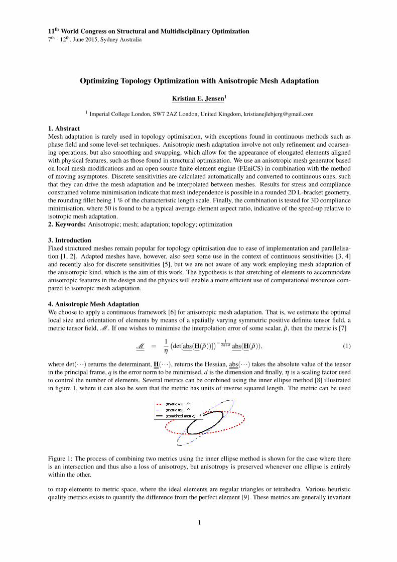
where det(· · ·) returns the determinant, H(· · ·), returns the Hessian, abs(· · ·) takes the absolute value of the tensorin the principal frame, q is the error norm to be minimised, d is the dimension and finally, η is a scaling factor usedto control the number of elements. Several metrics can be combined using the inner ellipse method [8] illustratedin figure 1, where it can also be seen that the metric has units of inverse squared length. The metric can be used

Figure 1: The process of combining two metrics using the inner ellipse method is shown for the case where thereis an intersection and thus also a loss of anisotropy, but anisotropy is preserved whenever one ellipse is entirelywithin the other.

to map elements to metric space, where the ideal elements are regular triangles or tetrahedra. Various heuristicquality metrics exists to quantify the difference from the perfect element [9]. These metrics are generally invariant

1

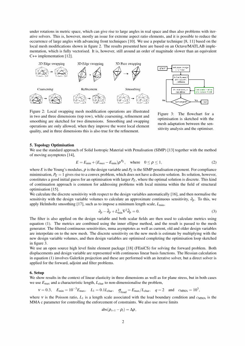
under rotations in metric space, which can give rise to large angles in real space and thus also problems with iter-ative solvers. This is, however, mostly an issue for extreme aspect ratio elements, and it is possible to reduce theoccurrence of large angles with advancing front techniques [10]. We use a popular technique [8, 11] based on thelocal mesh modifications shown in figure 2. The results presented here are based on an Octave/MATLAB imple-mentation, which is fully vectorised. It is, however, still around an order of magnitude slower than an equivalentC++ implementation [12].

Figure 2: Local swapping mesh modification operations are illustratedin two and three dimensions (top row), while coarsening, refinement andsmoothing are sketched for two dimensions. Smoothing and swappingoperations are only allowed, when they improve the worst local elementquality, and in three dimensions this is also true for the refinement.

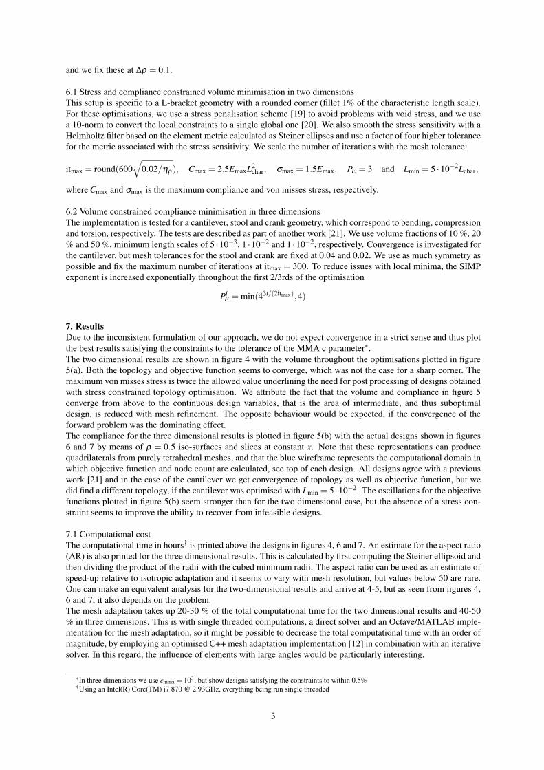
Figure 3: The flowchart for aoptimisation is sketched with themesh adaptation between the sen-sitivity analysis and the optimiser.

5. Topology OptimisationWe use the standard approach of Solid Isotropic Material with Penalisation (SIMP) [13] together with the methodof moving asymptotes [14],

E = Emin +(Emax −Emin)ρPE , where 0 ≤ ρ ≤ 1, (2)

where E is the Young’s modulus, ρ is the design variable and PE is the SIMP penalisation exponent. For complianceminimisation, PE = 1 gives rise to a convex problem, which does not have a discrete solution. Its solution, however,constitutes a good initial guess for an optimisation with larger PE , where the optimal solution is discrete. This kindof continuation approach is common for addressing problems with local minima within the field of structuraloptimisation [15].We calculate the discrete sensitivity with respect to the design variables automatically [16], and then normalise thesensitivity with the design variable volumes to calculate an approximate continuous sensitivity, ∂ρ . To this, weapply Helmholtz smoothing [17], such as to impose a minimum length scale, Lmin,

∂ρ − ∂ρ +L2min∇

2∂ρ = 0. (3)

The filter is also applied on the design variable and both scalar fields are then used to calculate metrics usingequation (1). The metrics are combined using the inner ellipse method, and the result is passed to the meshgenerator. The filtered continuous sensitivities, mma asymptotes as well as current, old and older design variablesare interpolate on to the new mesh. The discrete sensitivity on the new mesh is estimate by multiplying with thenew design variable volumes, and then design variables are optimised completing the optimisation loop sketchedin figure 3.We use an open source high level finite element package [18] (FEniCS) for solving the forward problem. Bothdisplacements and design variable are represented with continuous linear basis functions. The Hessian calculationin equation (1) involves Galerkin projection and these are performed with an iterative solver, but a direct solver isapplied for the forward, adjoint and filter problems.

6. SetupWe show results in the context of linear elasticity in three dimensions as well as for plane stress, but in both caseswe use Emax and a characteristic length, Lchar to non-dimensionalise the problem,

ν = 0.3, Emin = 10−3Emax, L1 = 0.1Lchar, σload

= Emax/Lchar, q = 2 and cMMA = 103,

where ν is the Poisson ratio, L1 is a length scale associated with the load boundary condition and cMMA is theMMA c parameter for controlling the enforcement of constraints. We also use move limits

abs(ρi+1 −ρi) = ∆ρ,

2

and we fix these at ∆ρ = 0.1.

6.1 Stress and compliance constrained volume minimisation in two dimensionsThis setup is specific to a L-bracket geometry with a rounded corner (fillet 1% of the characteristic length scale).For these optimisations, we use a stress penalisation scheme [19] to avoid problems with void stress, and we usea 10-norm to convert the local constraints to a single global one [20]. We also smooth the stress sensitivity with aHelmholtz filter based on the element metric calculated as Steiner ellipses and use a factor of four higher tolerancefor the metric associated with the stress sensitivity. We scale the number of iterations with the mesh tolerance:

itmax = round(600√

0.02/ηρ), Cmax = 2.5EmaxL2char, σmax = 1.5Emax, PE = 3 and Lmin = 5 ·10−2Lchar,

where Cmax and σmax is the maximum compliance and von misses stress, respectively.

6.2 Volume constrained compliance minimisation in three dimensionsThe implementation is tested for a cantilever, stool and crank geometry, which correspond to bending, compressionand torsion, respectively. The tests are described as part of another work [21]. We use volume fractions of 10 %, 20% and 50 %, minimum length scales of 5 ·10−3, 1 ·10−2 and 1 ·10−2, respectively. Convergence is investigated forthe cantilever, but mesh tolerances for the stool and crank are fixed at 0.04 and 0.02. We use as much symmetry aspossible and fix the maximum number of iterations at itmax = 300. To reduce issues with local minima, the SIMPexponent is increased exponentially throughout the first 2/3rds of the optimisation

PiE = min(43i/(2itmax),4).

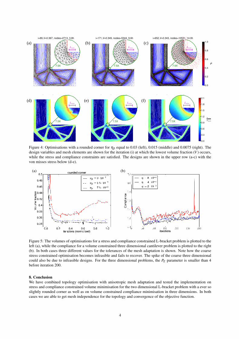
7. ResultsDue to the inconsistent formulation of our approach, we do not expect convergence in a strict sense and thus plotthe best results satisfying the constraints to the tolerance of the MMA c parameter∗.The two dimensional results are shown in figure 4 with the volume throughout the optimisations plotted in figure5(a). Both the topology and objective function seems to converge, which was not the case for a sharp corner. Themaximum von misses stress is twice the allowed value underlining the need for post processing of designs obtainedwith stress constrained topology optimisation. We attribute the fact that the volume and compliance in figure 5converge from above to the continuous design variables, that is the area of intermediate, and thus suboptimaldesign, is reduced with mesh refinement. The opposite behaviour would be expected, if the convergence of theforward problem was the dominating effect.The compliance for the three dimensional results is plotted in figure 5(b) with the actual designs shown in figures6 and 7 by means of ρ = 0.5 iso-surfaces and slices at constant x. Note that these representations can producequadrilaterals from purely tetrahedral meshes, and that the blue wireframe represents the computational domain inwhich objective function and node count are calculated, see top of each design. All designs agree with a previouswork [21] and in the case of the cantilever we get convergence of topology as well as objective function, but wedid find a different topology, if the cantilever was optimised with Lmin = 5 ·10−2. The oscillations for the objectivefunctions plotted in figure 5(b) seem stronger than for the two dimensional case, but the absence of a stress con-straint seems to improve the ability to recover from infeasible designs.

7.1 Computational costThe computational time in hours† is printed above the designs in figures 4, 6 and 7. An estimate for the aspect ratio(AR) is also printed for the three dimensional results. This is calculated by first computing the Steiner ellipsoid andthen dividing the product of the radii with the cubed minimum radii. The aspect ratio can be used as an estimate ofspeed-up relative to isotropic adaptation and it seems to vary with mesh resolution, but values below 50 are rare.One can make an equivalent analysis for the two-dimensional results and arrive at 4-5, but as seen from figures 4,6 and 7, it also depends on the problem.The mesh adaptation takes up 20-30 % of the total computational time for the two dimensional results and 40-50% in three dimensions. This is with single threaded computations, a direct solver and an Octave/MATLAB imple-mentation for the mesh adaptation, so it might be possible to decrease the total computational time with an order ofmagnitude, by employing an optimised C++ mesh adaptation implementation [12] in combination with an iterativesolver. In this regard, the influence of elements with large angles would be particularly interesting.

∗In three dimensions we use cmma = 103, but show designs satisfying the constraints to within 0.5%†Using an Intel(R) Core(TM) i7 870 @ 2.93GHz, everything being run single threaded

3

7.5X

Lmin

i=89,V=0.367, nodes=2713, 3.8h

(a)

7.5X

Lmin

i=171,V=0.349, nodes=5344, 9.6h

(b)

7.5X

Lmin

i=652,V=0.343, nodes=10531, 14.0h

(c)

ρ

0.0

0.2

0.4

0.6

0.8

1.0

7.5X

Lmin

i=89,V=0.367, nodes=2713, 3.8h

(d)

7.5X

Lmin

i=171,V=0.349, nodes=5344, 9.6h

(e)

7.5X

Lmin

i=652,V=0.343, nodes=10531, 14.0h

(f)

σmiss

σmax

0.0

0.3

0.6

0.9

1.2

1.5

1.8

2.1

Figure 4: Optimisations with a rounded corner for ηρ equal to 0.03 (left), 0.015 (middle) and 0.0075 (right). Thedesign variables and mesh elements are shown for the iteration (i) at which the lowest volume fraction (V ) occurs,while the stress and compliance constraints are satisfied. The designs are shown in the upper row (a-c) with thevon misses stress below (d-e).

(a) (b)

Figure 5: The volumes of optimisations for a stress and compliance constrained L-bracket problem is plotted to theleft (a), while the compliance for a volume constrained three dimensional cantilever problem is plotted to the right(b). In both cases three different values for the tolerances of the mesh adaptation is shown. Note how the coarsestress constrained optimisation becomes infeasible and fails to recover. The spike of the coarse three dimensionalcould also be due to infeasible designs. For the three dimensional problems, the PE parameter is smaller than 4before iteration 200.

8. ConclusionWe have combined topology optimisation with anisotropic mesh adaptation and tested the implementation onstress and compliance constrained volume minimisation for the two dimensional L-bracket problem with a ever soslightly rounded corner as well as on volume constrained compliance minimisation in three dimensions. In bothcases we are able to get mesh independence for the topology and convergence of the objective function.

4

9. AcknowledgementThis is work supported by the Villum Foundation.

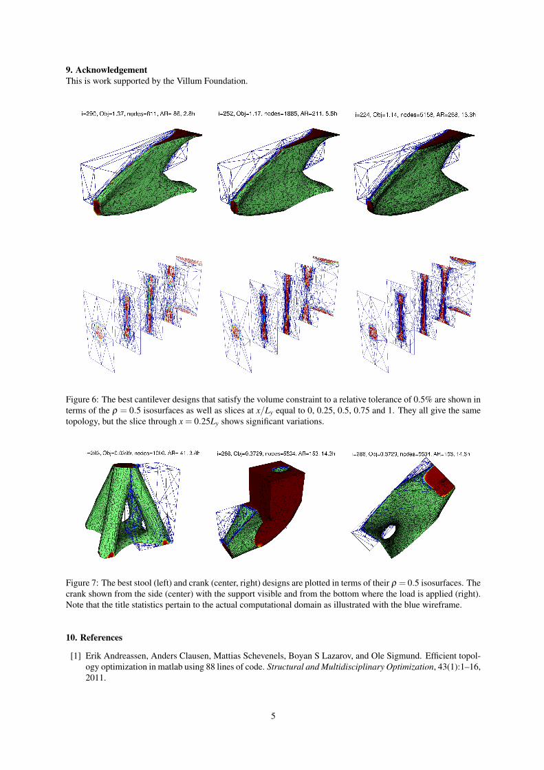
Figure 6: The best cantilever designs that satisfy the volume constraint to a relative tolerance of 0.5% are shown interms of the ρ = 0.5 isosurfaces as well as slices at x/Ly equal to 0, 0.25, 0.5, 0.75 and 1. They all give the sametopology, but the slice through x = 0.25Ly shows significant variations.

Figure 7: The best stool (left) and crank (center, right) designs are plotted in terms of their ρ = 0.5 isosurfaces. Thecrank shown from the side (center) with the support visible and from the bottom where the load is applied (right).Note that the title statistics pertain to the actual computational domain as illustrated with the blue wireframe.

10. References

[1] Erik Andreassen, Anders Clausen, Mattias Schevenels, Boyan S Lazarov, and Ole Sigmund. Efficient topol-ogy optimization in matlab using 88 lines of code. Structural and Multidisciplinary Optimization, 43(1):1–16,2011.

5

[2] Niels Aage, Erik Andreassen, and Boyan Stefanov Lazarov. Topology optimization using petsc. Structuraland Multidisciplinary Optimization, 2015.

[3] Mathias Wallin, Matti Ristinmaa, and Henrik Askfelt. Optimal topologies derived from a phase-field method.Structural and Multidisciplinary Optimization, 45(2):171–183, 2012.

[4] Samuel Amstutz and Antonio A Novotny. Topological optimization of structures subject to von mises stressconstraints. Structural and Multidisciplinary Optimization, 41(3):407–420, 2010.

[5] Asger Nyman Christiansen, J Andreas Bærentzen, Morten Nobel-Jørgensen, Niels Aage, and Ole Sigmund.Combined shape and topology optimization of 3d structures. Computers & Graphics, 46:25–35, 2015.

[6] Adrien Loseille and Frederic Alauzet. Continuous mesh framework part i: well-posed continuous interpola-tion error. SIAM Journal on Numerical Analysis, 49(1):38–60, 2011.

[7] Long Chen, Pengtao Sun, and Jinchao Xu. Optimal anisotropic meshes for minimizing interpolation errorsin L p-norm. Mathematics of Computation, 76(257):179–204, 2007.

[8] CC Pain, AP Umpleby, CRE De Oliveira, and AJH Goddard. Tetrahedral mesh optimisation and adaptivityfor steady-state and transient finite element calculations. Computer Methods in Applied Mechanics andEngineering, 190(29):3771–3796, 2001.

[9] Yu V Vasilevski and KN Lipnikov. Error bounds for controllable adaptive algorithms based on a hessianrecovery. Computational Mathematics and Mathematical Physics, 45(8):1374–1384, 2005.

[10] Adrien Loseille. Metric-orthogonal anisotropic mesh generation. Procedia Engineering, 82:403–415, 2014.

[11] Xiangrong Li, Mark S Shephard, and Mark W Beall. 3d anisotropic mesh adaptation by mesh modification.Computer methods in applied mechanics and engineering, 194(48):4915–4950, 2005.

[12] Georgios Rokos, Gerard J Gorman, James Southern, and Paul HJ Kelly. A thread-parallel algorithm foranisotropic mesh adaptation. arXiv preprint arXiv:1308.2480, 2013.

[13] Martin Philip Bendsoe and Ole Sigmund. Topology optimization: theory, methods and applications. Springer,2003.

[14] Krister Svanberg. The method of moving asymptotesa new method for structural optimization. Internationaljournal for numerical methods in engineering, 24(2):359–373, 1987.

[15] Albert A Groenwold and LFP Etman. A quadratic approximation for structural topology optimization. Inter-national Journal for Numerical Methods in Engineering, 82(4):505–524, 2010.

[16] Patrick E Farrell, David A Ham, Simon W Funke, and Marie E Rognes. Automated derivation of the adjointof high-level transient finite element programs. SIAM Journal on Scientific Computing, 35(4):C369–C393,2013.

[17] Boyan Stefanov Lazarov and Ole Sigmund. Filters in topology optimization based on helmholtz-type differ-ential equations. International Journal for Numerical Methods in Engineering, 86(6):765–781, 2011.

[18] Anders Logg, Kent-Andre Mardal, Garth N. Wells, et al. Automated Solution of Differential Equations by theFinite Element Method. Springer, 2012.

[19] GD Cheng and Xiao Guo. ε-relaxed approach in structural topology optimization. Structural Optimization,13(4):258–266, 1997.

[20] Pierre Duysinx and Ole Sigmund. New developments in handling stress constraints in optimal material dis-tribution. In Proc of the 7th AIAA/USAF/NASAISSMO Symp on Multidisciplinary Analysis and Optimization,volume 1, pages 1501–1509, 1998.

[21] Thomas Borrvall and Joakim Petersson. Large-scale topology optimization in 3d using parallel computing.Computer methods in applied mechanics and engineering, 190(46):6201–6229, 2001.

6