391
Optimum Signal Processing

OptimumSignal Processing


OptimumSignal ProcessingAn Introduction
Second Edition
Sophocles J. Orfanidis
Rutgers University
http://www.ece.rutgers.edu/~orfanidi/osp2e

To my parents
John and Clio Orfanidis
Copyright © 1988 by McGraw-Hill Publishing CompanyCopyright © 1996–2007 by Sophocles J. Orfanidis
This revised printing, first published in 2007, is a republication of the second edition ofthis book published by McGraw-Hill Publishing Company, New York, NY, in 1988 (ISBN0-07-047794-9), and also published earlier by Macmillan, Inc., New York, NY, 1988 (ISBN0-02-389380-X). All copyrights to this work reverted to Sophocles J. Orfanidis in 1996.
All rights reserved. No parts of this publication may be reproduced, stored in a retrievalsystem, or transmitted in any form or by any means, electronic, mechanical, photocopy-ing, recording or otherwise, without the prior written permission of the author.
MATLAB©R is a registered trademark of The MathWorks, Inc.
Web page: http://www.ece.rutgers.edu/~orfanidi/osp2e
ISBN-13: 978-0-9793713-0-1 (softcover)ISBN-10: 0-9793713-0-9
ISBN-13: 978-0-9793713-1-8 (hardcover)ISBN-10: 0-9793713-1-7

Contents
Preface ix
1 Random Signals 1
1.1 Probability Density, Mean, Variance, 11.2 Chebyshev’s Inequality, 21.3 Joint and Conditional Densities, and Bayes’ Rule, 41.4 Correlation Canceling, 71.5 Gram-Schmidt Orthogonalization, 111.6 Partial Correlations, 191.7 Forward/Backward Prediction and LU/UL Factorization, 231.8 Random Signals, 381.9 Power Spectrum and Its Interpretation, 401.10 Sample Autocorrelation and the Periodogram, 421.11 Random Signal Models and Their Uses, 451.12 Filter Model of First Order Autoregressive Process, 511.13 Stability and Stationarity, 521.14 Parameter Estimation by the Maximum Likelihood Method, 531.15 Parameter Estimation by the Yule-Walker Method, 541.16 Linear Prediction and Signal Modeling, 561.17 Cramer–Rao Bound and Maximum Likelihood, 581.18 Problems, 631.19 References, 70
2 Some Signal Processing Applications 72
2.1 Filtering of Stationary Random Signals, 722.2 System Identification by Cross-Correlation Methods, 752.3 Noise Reduction and Signal Enhancement Filters, 762.4 Quantization Noise, 832.5 Statistical Treatment of Multiplier Roundoff Error, 842.6 Introduction to Linear Prediction, 862.7 Gapped Functions, Levinson and Schur Recursions, 912.8 Introduction to Data Compression and DPCM, 972.9 Problems, 1002.10 References, 104
3 Spectral Factorization 106
3.1 Minimum-Phase Signals and Filters, 1063.2 Partial Energy and Minimal Delay, 1073.3 Invariance of the Autocorrelation Function, 1083.4 Minimum-Delay Property, 1083.5 Minimum-Phase Property, 1093.6 Spectral Factorization Theorem, 1103.7 Minimum-Phase Property of the Prediction-Error Filter, 112
v
vi CONTENTS
3.8 Problems, 1133.9 References, 115
4 Linear Estimation of Signals 117
4.1 Linear and Nonlinear Estimation of Signals, 1184.2 Orthogonality and Normal Equations, 1214.3 Stationary Wiener Filter, 1254.4 Construction of the Wiener Filter by Prewhitening, 1274.5 Wiener Filter Example, 1294.6 Wiener Filter as Kalman Filter, 1304.7 Construction of the Wiener Filter by the Gapped Function, 1354.8 Construction of the Wiener Filter by Covariance Factorization, 1364.9 The Kalman Filter, 1394.10 Problems, 1424.11 References, 145
5 Linear Prediction 147
5.1 Pure Prediction and Signal Modeling, 1475.2 Autoregressive Models, 1505.3 Linear Prediction and the Levinson Recursion, 1525.4 Levinson’s Algorithm in Matrix Form, 1605.5 Autocorrelation Sequence Extensions, 1645.6 Split Levinson Algorithm, 1675.7 Analysis and Synthesis Lattice Filters, 1705.8 Alternative Proof of the Minimum-Phase Property, 1745.9 Orthogonality of Backward Prediction Errors—Cholesky Factorization, 1765.10 Schur Algorithm, 1805.11 Lattice Realizations of FIR Wiener Filters, 1865.12 Autocorrelation, Covariance, and Burg’s Methods, 1935.13 Dynamic Predictive Deconvolution—Waves in Layered Media, 1985.14 Least-Squares Waveshaping and Spiking Filters, 2115.15 Problems, 2215.16 References, 227
6 Spectrum Estimation 234
6.1 Spectrum Estimation by Autoregressive Modeling, 2346.2 Spectral Analysis of Sinusoids in Noise, 2366.3 Superresolution Array Processing, 2486.4 Eigenvector Methods, 2596.5 MUSIC method, 2616.6 Minimum-Norm Method, 2646.7 Reduced-Order Method, 2676.8 Maximum Likelihood Method, 2706.9 ESPRIT Method, 2716.10 Spatial Smoothing, 2736.11 Asymptotic Properties, 2766.12 Problems, 2846.13 References, 290
7 Adaptive Filters 297
7.1 Adaptive Implementation of Wiener Filters, 2977.2 Correlation Canceler Loop (CCL), 3007.3 The Widrow-Hoff LMS Adaptation Algorithm, 3027.4 Adaptive Linear Combiner, 3067.5 Adaptive FIR Wiener Filter, 308

7.6 Speed of Convergence, 3117.7 Adaptive Channel Equalizers, 3147.8 Adaptive Echo Cancelers, 3157.9 Adaptive Noise Canceling, 3167.10 Adaptive Line Enhancer, 3187.11 Adaptive Linear Prediction, 3207.12 Adaptive Implementation of Pisarenko’s Method, 3227.13 Gradient Adaptive Lattice Filters, 3277.14 Adaptive Gram-Schmidt Preprocessors, 3347.15 Rank-One Modification of Covariance Matrices, 3397.16 RLS Adaptive Filters, 3507.17 Fast RLS Filters, 3537.18 RLS Lattice Filters, 3567.19 Problems, 3617.20 References, 365
8 Appendices 372
8.1 Fortran and C Functions, 3728.2 MATLAB Functions, 373
Index 374


Preface
Digital signal processing is currently in a period of rapid growth caused by recentadvances in VLSI technology. This is especially true of three areas of optimum signal pro-cessing; namely, real-time adaptive signal processing, eigenvector methods of spectrumestimation, and parallel processor implementations of optimum filtering and predictionalgorithms.
In this edition the book has been brought up to date by increasing the emphasison the above areas and including several new developments. The major additions are:a unified presentation of the fast recursive least-squares algorithms for adaptive pro-cessing; the discussion of several eigenvector methods of spectrum estimation such asMUSIC, minimum-norm, ESPRIT, spatial smoothing for coherent signals, and others; anddiscussion of the Schur algorithm for linear prediction admitting efficient parallel imple-mentations, and the more efficient split Schur and split Levinson algorithms. Moreover,older but basic material has been added such as an expanded discussion of Kalmanfiltering and discussion of classical statistical estimation concepts such as maximumlikelihood, Cramer-Rao bound, and asymptotic statistical properties applied to linearprediction and eigenstructure methods.
Two new sections have been added to Chapter 1 with the aim of strengthening thediscussion of statistical concepts while at the same time emphasizing the unity of ideasof optimum signal processing. The first section, dealing with forward and backwardprediction, develops further the geometrical point of view of random variables and lin-ear estimation and provides a preliminary introduction to a large number of methodsthat have become important tools in signal processing; namely, Levinson’s and Schur’salgorithms, fast matrix factorizations, Gram-Schmidt orthogonalizations, lattice real-izations of linear predictors and Wiener filters, and fast RLS algorithms. The secondsection discusses the properties of maximum likelihood estimators and gives a deriva-tion of the Cramer-Rao bound using correlation canceling methods. The results of thissection are used later to derive the asymptotic statistical properties of linear predictorsand eigenstructure methods.
Chapter 2 has been revised to include a preliminary introduction to the Schur algo-rithm using a gapped function approach. Chapter 3 remains unchanged. A new sectionon Kalman filtering has been added to Chapter 4 that includes a derivation of the Kalmanfilter, a geometrical interpretation of it, and discussion of its asymptotic convergenceproperties.
Three new sections have been added to Chapter 5. The first deals with the problemof autocorrelation sequence extensions, such as the maximum entropy or autoregres-sive extensions, and discusses the case of singular autocorrelation matrices, their sinu-soidal representations, and their connection to Pisarenko’s harmonic retrieval method.The second section contains a discussion of the recently developed split or immitance-domain Levinson algorithm which is fifty percent more efficient than the conventionalLevinson algorithm. The third section presents the Schur algorithm for linear predic-tion which has received a lot of attention recently because of its efficient parallel im-

x PREFACE
plementations, and discusses its application to fast matrix factorizations. The split orimmitance-domain version of the Schur algorithm is also discussed.
The material on autoregressive spectrum estimation, spectral analysis of sinusoidsin noise, and superresolution array processing, has been separated from Chapter 5 toform a new Chapter 6. This chapter also includes new sections on several eigenstructuremethods and a section on the asymptotic statistical properties of such methods. Thefollowing methods are discussed: MUSIC, minimum-norm, reduced-order, maximumlikelihood, ESPRIT, and spatial smoothing for coherent signals.
The chapter on adaptive filtering, now Chapter 7, has been expanded considerably.It contains a revised discussion of the adaptive gradient lattice Wiener filter and itsspatial processing counterpart—the adaptive Gram-Schmidt array preprocessor basedon the modified Gram-Schmidt procedure. The last four sections are devoted to a uni-fied derivation of the exact recursive least-squares adaptation algorithms including theconventional RLS, fast Kalman and FAEST/FTF direct form versions, and RLS lattice ver-sions. We show first that the algebraic steps and computational reductions that makeall the fast versions possible are a direct consequence of the rank-one updating prop-erties of covariance matrices, and then apply the shift-invariance property to completethe derivation of the various RLS algorithms.
A new appendix has been added containing a discussion of uniform and gaussianrandom number generators and ways to improve them such as shuffling. The numberof subroutines discussed in the text has been tripled and the routines have been writtenboth in FORTRAN and C. Several new problems and computer experiments have beenadded, and a solutions manual is available through the publisher. The material in thisexpanded edition is now adequate for a two-semester graduate course on the subject.
I have tried in this edition to preserve the basic style and objectives of the book andwould like to thank the many colleagues and students who have given me their feedbackon the first edition. Working on the revision was a great deal of fun and it was madeeven more so by my three-year old son, John.
Sophocles J. Orfanidis1988
The content of the 2007 republication of this book remains the same as that of the1988 edition, except for some corrections, the deletion from the Appendix of the Fortranand C function listings, which are now available online, and the addition of MATLABversions of all the functions. A pdf version of the book, as well as all the functions, canbe downloaded freely from the web page:
http://www.ece.rutgers.edu/~orfanidi/osp2e
Sophocles J. Orfanidis2007

Preface to the First Edition
The purpose of this book is to provide an introduction to signal processing methodsthat are based on optimum Wiener filtering and least-squares estimation concepts. Suchmethods have a remarkably broad range of applications, ranging from the analysis andsynthesis of speech, data compression, image processing and modeling, channel equal-ization and echo cancellation in digital data transmission, geophysical signal processingin oil exploration, linear predictive analysis of EEG signals, modern methods of high-resolution spectrum estimation, and superresolution array processing, to adaptive sig-nal processing for sonar, radar, system identification, and adaptive control applications.The structure of the book is to present the Wiener filtering concept as the basic unify-ing theme that ties together the various signal processing algorithms and techniquescurrently used in the above applications.
The book is based on lecture notes for a second-semester graduate-level course onadvanced topics in digital signal processing that I have taught at Rutgers Universitysince 1979. The book is primarily addressed to beginning graduate students in elec-trical engineering, but it may also be used as a reference by practicing engineers whowant a concise introduction to the subject. The prerequisites for using the book are anintroductory course on digital signal processing, such as on the level of Oppenheim andSchafer’s book, and some familiarity with probability and random signal concepts, suchas on the level of Papoulis’ book.
Chapter 1 sets many of the objectives of the book and serves both as a review ofprobability and random signals and as an introduction to some of the basic conceptsupon which the rest of the text is built. These are the concept of correlation cancelingand its connection to linear mean-squared estimation, and the concept of Gram-Schmidtorthogonalization of random variables and its connection to linear prediction and signalmodeling. After a brief review of some pertinent material on random signals, such asautocorrelations, power spectra, and the periodogram and its improvements, we dis-cuss parametric signal models in which the random signal is modeled as the outputof a linear system driven by white noise and present an overview of the uses of suchmodels in signal analysis and synthesis, spectrum estimation, signal classification, anddata compression applications. A first-order autoregressive model is used to illustratemany of these ideas and to motivate some practical methods of extracting the modelparameters from actual data.
Chapter 2 is also introductory, and its purpose is to present a number of straightfor-ward applications and simulation examples that illustrate the practical usage of randomsignal concepts. The selected topics include simple designs for signal enhancement fil-ters, quantization noise in digital filters, and an introduction to linear prediction basedon the finite past. The last two topics are then merged into an introductory discussionof data compression by DPCM methods.
Chapter 3 introduces the concept of minimal phase signals and filters and its role inthe making of parametric signal models via spectral factorization. These methods areused in Chapter 4 for the solution of the Wiener filtering problem.

xii PREFACE
The basic concept of the Wiener filter as an optimum filter for estimating one signalfrom another is developed in Chapter 4. The Wiener filter is also viewed as a correlationcanceler and as an optimal signal separator. We consider both the stationary and non-stationary Wiener filters, as well as the more practical FIR Wiener filter. While discussinga simple first-order Wiener filter example, we take the opportunity to introduce someelementary Kalman filter concepts. We demonstrate how the steady-state Kalman filteris equivalent to the Wiener filter and how its solution may be obtained from the steady-state algebraic Riccati equation which effects the spectral factorization required in theWiener case. We also show how the Kalman filter may be thought of as the whiteningfilter of the observation signal and discuss its connection to the Gram-Schmidt orthogo-nalization and parametric signal models of Chapter 1. This chapter is mainly theoreticalin character. Practical implementations and applications of Wiener filters are discussedin Chapter 5 using block-processing methods and in Chapter 6 using real-time adaptiveprocessing techniques.
Chapter 5 begins with a discussion of the full linear prediction problem and its con-nection to signal modeling and continues with the problem of linear prediction basedon the finite past and its efficient solution via the Levinson recursion. We discuss theanalysis and synthesis lattice filters of linear prediction, as well as the lattice realizationsof more general Wiener filters that are based on the orthogonality property of the back-ward prediction errors. The autocorrelation, covariance, and Burg’s methods of linearpredictive analysis are presented, and their application to speech analysis and synthesisand to spectrum estimation is discussed. The problem of estimating the frequencies ofmultiple sinusoids in noise and the problem of resolving the directions of point-sourceemitters by spatial array processing are discussed. Four approaches to these problemsare presented, namely, the classical method based on the windowed autocorrelation,the maximum entropy method based on linear prediction, Capon’s maximum likelihoodmethod, and eigenvector-based methods. We also discuss the problem of wave propa-gation in layered media and its connection to linear prediction, and present the dynamicpredictive deconvolution procedure for deconvolving the multiple reverberation effectsof a layered structure from the knowledge of its reflection or transmission response.The chapter ends with a discussion of a least-squares reformulation of the Wiener fil-tering problem that can be used in the design of waveshaping and spiking filters fordeconvolution applications.
Real-time adaptive implementations of Wiener filters are discussed in Chapter 6.The basic operation of an adaptive filter is explained by means of the simplest possi-ble filter, namely, the correlation canceler loop, which forms the elementary buildingblock of higher order adaptive filters. The Widrow-Hoff LMS adaptation algorithm andits convergence properties are discussed next. Several applications of adaptive filtersare presented, such as adaptive noise canceling, adaptive channel equalization and echocancellation, adaptive signal separation and the adaptive line enhancer, adaptive spec-trum estimation based on linear prediction, and adaptive array processing. We alsodiscuss some recent developments, such as the adaptive implementation of Pisarenko’smethod of harmonic retrieval, and two alternative adaptation algorithms that offer veryfast speed of convergence, namely, recursive least-squares, and gradient lattice adaptivefilters.
The subject of Wiener filtering and linear estimation is vast. The selection of ma-terial in this book reflects my preferences and views on what should be included in anintroductory course on this subject. The emphasis throughout the book is on the signalprocessing procedures that grow out of the fundamental concept of Wiener filtering.An important ingredient of the book is the inclusion of several computer experimentsand assignments that demonstrate the successes and limitations of the various signalprocessing algorithms that are discussed. A set of FORTRAN 77 subroutines, designedto be used as a library, has been included in an appendix.

PREFACE xiii
I would like to thank my colleagues Professors T. G. Marshall and P. Sannuti for theirsupport. I am greatly indebted to Professor R. Peskin for making available his graphicssystem on which many of the simulation examples were run and to my graduate studentMs. L. M. Vail for her invaluable help in producing most of the computer graphs. Mostof all, I would like to thank my wife Monica, without whose love and affection this bookcould not have been written.
Sophocles J. Orfanidis


1Random Signals
1.1 Probability Density, Mean, Variance
In this section, we present a short review of probability concepts. It is assumed that thestudent has had a course on the subject on the level of Papoulis’ book [1].
Let x be a random variable having probability density p(x). Its mean, variance, andsecond moment are defined by the expectation values
m = E[x] =∫∞−∞xp(x)dx = mean
σ2 = var(x)= E[(x−m)2] = ∫∞
−∞(x−m)2p(x)dx = variance
E[x2] =∫∞−∞x2p(x)dx = second moment
These quantities are known as second-order statistics of the random variable x. Theirimportance is linked with the fact that most optimal filter design criteria require knowl-edge only of the second-order statistics and do not require more detailed knowledge,such as probability densities. It is of primary importance, then, to be able to extractsuch quantities from the actual measured data.
The probability that the random variable x will assume a value within an interval ofvalues [a, b] is given by
Prob[a ≤ x ≤ b]=∫ bap(x)dx = shaded area
The probability density is always normalized to unity by∫∞−∞p(x)dx = 1
which states that the probability of x taking a value somewhere within its range ofvariation is unity, that is, certainty. This property also implies
σ2 = E[(x−m)2] = E[x2]−m2
Example 1.1.1: Gaussian, or normal, distribution

2 1. Random Signals
p(x)= 1√2πσ
exp[−(x−m)2/2σ2
]
Example 1.1.2: Uniform distribution
p(x)=⎧⎨⎩1/Q , for −Q/2 ≤ x ≤ Q/2
0, otherwise
Its variance is σ2 = Q2/12. ��
Both the gaussian and the uniform distributions will prove to be important examples.In typical signal processing problems of designing filters to remove or separate noisefrom signal, it is often assumed that the noise interference is gaussian. This assumptionis justified on the grounds of the central limit theorem, provided that the noise arisesfrom many different noise sources acting independently of each other.
The uniform distribution is also important. In digital signal processing applications.the quantization error arising from the signal quantization in the A/D converters, or theroundoff error arising from the finite accuracy of the internal arithmetic operations indigital filters, can often be assumed to be uniformly distributed.
Every computer provides system routines for the generation of random numbers.For example, the routines RANDU and GAUSS of the IBM Scientific Subroutine Packagegenerate uniformly distributed random numbers over the interval [0,1], and gaussian-distributed numbers, respectively. GAUSS calls RANDU twelve times, thus generatingtwelve independent uniformly distributed random numbers x1, x2, . . . , x12. Then, theirsum x = x1+x2+· · ·+x12, will be approximately gaussian, as guaranteed by the centrallimit theorem. It is interesting to note that the variance of x is unity, as it follows fromthe fact that the variance of each xi, is 1/12:
σ2x = σ2
x1+σ2
x2+ · · · +σ2
x12= 1
12+ 1
12+ · · · + 1
12= 1
The mean of x is 12/2 = 6. By shifting and scaling x, one can obtain a gaussian-distributed random number of any desired mean and variance. Appendix A contains adiscussion of random number generators and methods to improve them, such as shuf-fling or using several generators in combination. A number of FORTRAN and C routinesfor generating uniform and gaussian random numbers are included.
1.2 Chebyshev’s Inequality
The variance σ2 of a random variable x is a measure of the spread of the x-valuesabout their mean. This intuitive interpretation of the variance is a direct consequenceof Chebyshev’s inequality, which states that the x-values tend to cluster about theirmean in the sense that the probability of a value not occurring in the near vicinity of themean is small; and it is smaller the smaller the variance.

1.2. Chebyshev’s Inequality 3
More precisely, for any probability density p(x) and any Δ > 0, the probability thatx will fall outside the interval of values [m−Δ,m+Δ] is bounded by σ2/Δ2. Thus, forfixed Δ, as the variance σ2 becomes smaller, the x-values tend to cluster more narrowlyabout the mean. In the extreme limiting case of a deterministic variable x = m, thedensity becomes infinitely narrow, p(x)= δ(x−m), and has zero variance.
Prob[|x−m| ≥ Δ] ≤ σ2
Δ2
(Chebyshev’s Inequality)
Chebyshev’s inequality is especially important in proving asymptotic convergenceresults for sample estimates of parameters. For example, considerN independent sam-ples {x1, x2, . . . , xN} drawn from a gaussian probability distribution of mean m andvariance σ2. The sample estimate of the mean is
m = 1
N(x1 + x2 + · · · + xN) (1.2.1)
Being a sum of N gaussian random variables, m will itself be a gaussian randomvariable. Its probability density is completely determined by the corresponding meanand variance. These are found as follows.
E[m]= 1
N(E[x1]+E[x2]+· · · + E[xN]
) = 1
N(m+m+ · · · +m)=m
Therefore, m is an unbiased estimator of m. However, the goodness of m as an es-timator must be judged by how small its variance is—the smaller the better, by Cheby-shev’s inequality. By the assumption of independence, we have
var(m)= E[(m−m)2] = 1
N2
(σ2x1+σ2
x2+ · · · +σ2
xN) = 1
N2
(Nσ2) = σ2
N(1.2.2)
Thus, m is also a consistent estimator of m in the sense that its variance tends tozero as the number of samples N increases. The values of m will tend to cluster moreand more closely about the true value ofm asN becomes larger. Chebyshev’s inequalityimplies that the probability of m falling outside any fixed neighborhood ofm will tendto zero for large N. Equivalently, m will converge to m with probability one. This canalso be seen from the probability density of m, which is the gaussian
p(m)= N1/2
(2π)1/2σexp
[− N2σ2
(m−m)2]In the limit of large N, this density tends to the infinitely narrow delta function
density p(m)= δ(m − m). In addition to the sample mean, we may also computesample estimates of the variance σ2 by
σ2 = 1
N
N∑i=1
(xi − m)2 (1.2.3)
It is easily shown [2,3] that this estimator is slightly biased. But for large N, it isasymptotically unbiased and consistent as can be seen from its mean and variance:
E[σ2]= N − 1
Nσ2 , var(σ2)= N − 1
N22σ4 (1.2.4)
An unbiased and consistent estimator of σ2 is the standard deviation defined by

4 1. Random Signals
s2 = 1
N − 1
N∑i=1
(xi − m)2 (1.2.5)
It has E[s2]= σ2 and var(s2)= 2σ4/(N − 1) . In addition to the requirements ofasymptotic unbiasedness and consistency, a good estimator of a parameter must also bejudged in terms of its efficiency [2,3], which determines how closely the estimator meetsits Cramer-Rao bound. This is discussed in Section 1.17. We will see there that the es-timators (1.2.1) and (1.2.3)—being maximum likelihood estimators—are asymptoticallyefficient.
1.3 Joint and Conditional Densities, and Bayes’ Rule
Next, we discuss random vectors. A pair of two different random variables x = (x1, x2)may be thought of as a vector-valued random variable. Its statistical description is morecomplicated than that of a single variable and requires knowledge of the joint probabilitydensity p(x1, x2). The two random variables may or may not have any dependence oneach other. It is possible, for example, that if x2 assumes a particular value, then thisfact may influence, or restrict, the possible values that x1 can then assume.
A quantity that provides a measure for the degree of dependence of the two variableson each other is the conditional density p(x1|x2) of x1 given x2; and p(x2|x1) of x2 givenx1. These are related by Bayes’ rule
p(x1, x2)= p(x1|x2)p(x2)= p(x2|x1)p(x1)
More generally, Bayes’ rule for two events A and B is
p(A,B)= p(A|B)p(B)= p(B|A)p(A)
The two random variables x1 and x2 are independent of each other if they do notcondition each other in any way, that is, if
p(x1|x2)= p(x1) or p(x2|x1)= p(x2)
In other words, the occurrence of x2 does not in any way influence the variable x1.When two random variables are independent, their joint density factors into the productof single (marginal) densities:
p(x1, x2)= p(x1)p(x2)
The converse is also true. The correlation between x1 and x2 is defined by the expectationvalue
E[x1x2]=∫∫x1x2p(x1, x2)dx1dx2
When x1 and x2 are independent, the correlation also factors as E[x1x2]= E[x1]E[x2].
Example 1.3.1: Suppose x1 is related to x2 by
x1 = 5x2 + v
where v is a zero-mean, unit-variance, gaussian random variable assumed to be indepen-dent of x2. Determine the conditional density and conditional mean of x1 given x2.

1.3. Joint and Conditional Densities, and Bayes’ Rule 5
Solution: The randomness of x1 arises both from the randomness of x2 and the randomness ofv. But if x2 takes on a particular value, then the randomness of x1 will arise only from v.Identifying elemental probabilities we have
p(x1|x2)dx1 = p(v)dv = (2π)−1/2exp(−1
2v2
)dv
But, dx1 = dv and v = x1 − 5x2. Therefore,
p(x1|x2)= (2π)−1/2exp[−1
2(x1 − 5x2)2
]The conditional mean is the mean of x1 with respect to the density p(x1|x2). It is evidentfrom the above gaussian expression that the conditional mean is E[x1|x2]= 5x2. This canalso be found directly as follows.
E[x1|x2]= E[(5x2 + v)|x2
] = 5x2 + E[v|x2]= 5x2
where we used the independence of v and x2 to replace the conditional mean of v with itsunconditional mean, which was given to be zero, that is, E[v|x2]= E[v]= 0. ��
The concept of a random vector generalizes to any dimension. A vector ofN randomvariables
x =
⎡⎢⎢⎢⎢⎢⎣x1
x2
...xN
⎤⎥⎥⎥⎥⎥⎦requires knowledge of the joint density
p(x)= p(x1, x2, . . . , xN) (1.3.1)
for its complete statistical description. The second-order statistics of x are its mean, itscorrelation matrix, and its covariance matrix, defined by
m = E[x] , R = E[xxT] , Σ = E[(x−m)(x−m)T
](1.3.2)
where the superscript T denotes transposition, and the expectation operations are de-fined in terms of the joint density (1.3.1); for example,
E[x]=∫
xp(x)dNx
where dNx = dx1dx2 · · ·dxN denotes the corresponding N-dimensional volume ele-ment. The ijth matrix element of the correlation matrix R is the correlation betweenthe ith random variable xi with the jth random variable xj, that is, Rij = E[xixj] . It iseasily shown that the covariance and correlation matrices are related by
Σ = R−mmT
When the mean is zero, R and Σ coincide. Both R and Σ are symmetric positive semi-definite matrices.
Example 1.3.2: The probability density of a gaussian random vector x = [x1, x2, . . . , xN]T iscompletely specified by its mean m and covariance matrix Σ, that is,
p(x)= 1
(2π)N/2(detΣ)1/2 exp[−1
2(x−m)TΣ−1(x−m)
]

6 1. Random Signals
Example 1.3.3: Under a linear transformation, a gaussian random vector remains gaussian. Letx be a gaussian random vector of dimension N, mean mx, and covariance Σx. Show thatthe linearly transformed vector
ξξξ = Bx where B is a nonsingular N×N matrix
is gaussian-distributed with mean and covariance given by
mξ = Bmx , Σξ = BΣxBT (1.3.3)
The relationships (1.3.3) are valid also for non-gaussian random vectors. They are easilyderived as follows:
E[ξξξ]= E[Bx]= BE[x] , E[ξξξξξξT]= E[Bx(Bx)T]= BE[xxT]BT
The probability density pξ(ξξξ) is related to the density px(x) by the requirement that,under the above change of variables, they both yield the same elemental probabilities:
pξ(ξξξ)dNξξξ = px(x)dNx (1.3.4)
Since the Jacobian of the transformation from x to ξξξ is dNξξξ = |detB|dNx, we obtainpξ(ξξξ)= px(x)/|detB|. Noting the invariance of the quadratic form
(ξξξ−mξ)TΣ−1ξ (ξξξ−mξ) = (x−mx)TBT(BΣxBT)−1B(x−mx)
= (x−mx)TΣ−1x (x−mx)
and that detΣξ = det(BΣxBT)= (detB)2detΣx, we obtain
pξ(ξξξ)= 1
(2π)N/2(detΣξ)1/2 exp[−1
2(ξξξ−mξ)TΣ−1
ξ (ξξξ−mξ)]
Example 1.3.4: Consider two zero-mean random vectors x and y of dimensions N and M, re-spectively. Show that if they are uncorrelated and jointly gaussian, then they are alsoindependent of each other. That x and y are jointly gaussian means that the (N+M)-dimensional joint vector z =
[xy
]is zero-mean and gaussian, that is,
p(z)= 1
(2π)(N+M)/2(detRzz)1/2 exp[−1
2zTR−1
zz z]
where the correlation (covariance) matrix Rzz is
Rzz = E[[
xy
][xT,yT]
]=
[E[xxT] E[xyT]E[yxT] E[yyT]
]=
[Rxx RxyRyx Ryy
]
If x and y are uncorrelated, that is, Rxy = E[xyT]= 0, then the matrix Rzz becomes blockdiagonal and the quadratic form of the joint vector becomes the sum of the individualquadratic forms:
zTR−1zz z = [xT,yT]
[R−1xx 00 R−1
yy
][xy
]= xTR−1
xx x+ yTR−1yyy
Since Rxy = 0 also implies that detRzz = (detRxx)(detRyy), it follows that the jointdensity p(z)= p(x,y) factors into the marginal densities:
p(x,y)= p(x)p(y)
which shows the independence of x and y.

1.4. Correlation Canceling 7
Example 1.3.5: Given a random vector x with mean m and covariance Σ, show that the bestchoice of a deterministic vector x which minimizes the quantity
Ree = E[eeT]= minimum , where e = x− x,
is the mean m itself, that is, x = m. Also show that for this optimal choice of x, the actualminimum value of the quantity Ree is the covariance Σ. This property is easily shown byworking with the deviation of x from the mean m, that is, let
x = m+ΔΔΔ
Then, the quantity Ree becomes
Ree = E[eeT]= E[(x−m−ΔΔΔ)(x−m−ΔΔΔ)T
]= E[
(x−m)(x−m)T]−ΔΔΔE[xT −mT]−E[x−m]ΔΔΔ+ΔΔΔΔΔΔT
= Σ +ΔΔΔΔΔΔT
where we used the fact that E[x−m]= E[x]−m = 0. Since the matrix ΔΔΔΔΔΔT is nonnegative-definite, it follows that Ree, will be minimized when ΔΔΔ = 0, and in this case the minimumvalue will be Rmin
ee = Σ.
Since Ree is a matrix, the sense in which it is minimized must be clarified. The statementthatRee is greater thanRmin
ee means that the differenceRee−Rminee is a positive semi-definite
(and symmetric) matrix, and therefore we have for the scalar quantities: aTReea ≥ aTRminee a
for any vector a. ��
1.4 Correlation Canceling
The concept of correlation canceling plays a central role in the development of manyoptimum signal processing algorithms, because a correlation canceler is also the bestlinear processor for estimating one signal from another.
Consider two zero-mean random vectors x and y of dimensions N and M, respec-tively. If x and y are correlated with each other in the sense that Rxy = E[xyT]= 0, thenwe may remove such correlations by means of a linear transformation of the form
e = x−Hy (1.4.1)
where theN×MmatrixHmust be suitably chosen such that the new pair of vectors e,yare no longer correlated with each other, that is, we require
Rey = E[eyT]= 0 (1.4.2)
Using Eq. (1.4.1), we obtain
Rey = E[eyT]= E[(x−Hy)yT
] = E[xyT]−HE[yyT]= Rxy −HRyyThen, the condition Rey = 0 immediately implies that
H = RxyR−1yy = E[xyT]E[yyT]−1 (1.4.3)
Using Rey = 0, the covariance matrix of the resulting vector e is easily found to be
Ree = E[eeT]= E[e(xT − yTH)
] = Rex −ReyHT = Rex = E[(x−Hy)xT
], or,
Ree = Rxx −HRyx = Rxx −RxyR−1yyRyx (1.4.4)

8 1. Random Signals
The vectorx = Hy = RxyR−1
yyy = E[xyT]E[yyT]−1y (1.4.5)
obtained by linearly processing the vector y by the matrix H is called the linear regres-sion, or orthogonal projection, of x on the vector y. In a sense to be made precise later,x also represents the best “copy,” or estimate, of x that can be made on the basis of thevector y. Thus, the vector e = x−Hy = x− x may be thought of as the estimation error.
Actually, it is better to think of x = Hy not as an estimate of x but rather as anestimate of that part of x which is correlated with y. Indeed, suppose that x consists oftwo parts
x = x1 + x2
such that x1 is correlated with y, but x2 is not, that is, Rx2y = E[x2yT]= 0. Then,
Rxy = E[xyT]= E[(x1 + x2)yT]= Rx1y +Rx2y = Rx1y
and therefore,
x = RxyR−1yyy = Rx1yR
−1yyy = x1
The vector e = x− x = x1 + x2 − x1 = (x1 − x1)+x2 consists of the estimation error(x1−x1) of the x1-part plus the x2-part. Both of these terms are separately uncorrelatedfrom y. These operations are summarized in block diagram form in Fig. 1.1.
Fig. 1.1 Correlation canceler.
The most important feature of this arrangement is the correlation cancellation prop-erty which may be summarized as follows: If x has a part x1 which is correlated with y,then this part will tend to be canceled as much as possible from the output e. The linearprocessor H accomplishes this by converting y into the best possible copy x1 of x1 andthen proceeds to cancel it from the output. The output vector e is no longer correlatedwith y. The part x2 of x which is uncorrelated with y remains entirely unaffected. Itcannot be estimated in terms of y.
The correlation canceler may also be thought of as an optimal signal separator. In-deed, the output of the processor H is essentially the x1 component of x, whereas theoutput e is essentially the x2 component. The separation of x into x1 and x2 is optimalin the sense that the x1 component of x is removed as much as possible from e.
Next, we discuss the best linear estimator property of the correlation canceler. Thechoice H = RxyR−1
yy , which guarantees correlation cancellation, is also the choice thatgives the best estimate of x as a linear function of y in the form x = Hy. It is the bestestimate in the sense that it produces the lowest mean-square estimation error. To seethis, express the covariance matrix of the estimation error in terms of H, as follows:
Ree = E[eeT]= E[(x−Hy)(xT − yTHT)
] = Rxx −HRyx −RxyHT +HRyyHT (1.4.6)
Minimizing this expression with respect to H yields the optimum choice of H:
Hopt = RxyR−1yy
with the minimum value for Ree given by:
Rminee = Rxx −RxyR−1
yyRyx

1.4. Correlation Canceling 9
Any other value will result in a larger value for Ree. An alternative way to see this isto consider a deviation ΔH of H from its optimal value, that is, in (1.4.5) replace H by
H = Hopt +ΔH = RxyR−1yy +ΔH
Then Eq. (1.4.6) may be expressed in terms of ΔH as follows:
Ree = Rminee +ΔHRyy ΔHT
Since Ryy is positive definite, the second term always represents a nonnegative con-tribution above the minimum value Rmin
ee , so that(Ree −Rmin
ee)
is positive semi-definite.In summary, there are three useful ways to think of the correlation canceler:
1. Optimal estimator of x from y.2. Optimal canceler of that part of x which is correlated with y.3. Optimal signal separator
The point of view is determined by the application. The first view is typified byKalman filtering, channel equalization, and linear prediction applications. The secondview is taken in echo canceling, noise canceling, and sidelobe canceling applications.The third view is useful in the adaptive line enhancer, which is a method of adaptivelyseparating a signal into its broadband and narrowband components. All of these appli-cations are considered later on.
Example 1.4.1: If x and y are jointly gaussian, show that the linear estimate x = Hy is alsothe conditional mean E[x|y] of the vector x given the vector y. The conditional mean isdefined in terms of the conditional density p(x|y) of x given y as follows:
E[x|y]=∫
xp(x|y)dNx
Instead of computing this integral, we will use the results of Examples 1.3.3 and 1.3.4.The transformation from the jointly gaussian pair (x,y) to the uncorrelated pair (e,y) islinear: [
ey
]=
[IN −H0 IM
][xy
]
where IN and IM are the unit matrices of dimensions N and M, respectively. Therefore,Example 1.3.3 implies that the transformed pair (e,y) is also jointly gaussian. Further-more, since e and y are uncorrelated, it follows from Example 1.3.4 that they must beindependent of each other. The conditional mean of x can be computed by writing
x = x+ e = Hy+ e
and noting that if y is given, then Hy is no longer random. Therefore,
E[x|y]= E[(Hy+ e)|y] = Hy+ E[e|y]
Since e and y are independent, the conditional mean E[e|y] is the same as the uncondi-tional mean E[e], which is zero by the zero-mean assumption. Thus,
E[x|y]= Hy = RxyR−1yyy (jointly gaussian x and y) (1.4.7)
Example 1.4.2: Show that the conditional mean E[x|y] is the best unrestricted (i.e., not neces-sarily linear) estimate of x in the mean-square sense. The best linear estimate was obtainedby seeking the best linear function of y that minimized the error criterion (1.4.6), that is,we required a priori that the estimate was to be of the form x = Hy. Here, our task is more

10 1. Random Signals
general: find the most general function of y, x = x(y), which gives the best estimate of x,in the sense of producing the lowest mean-squared estimation error e = x− x(y),
Ree = E[eeT]= E[(x− x(y)
)(xT − x(y)T
)] = min
The functional dependence of x(y) on y is not required to be linear a priori. Usingp(x,y)=p(x|y)p(y), the above expectation may be written as
Ree =∫ (
x− x(y))(
xT − x(y)T)p(x,y)dNxdMy
=∫p(y)dMy
[∫ (x− x(y)
)(xT − x(y)T
)p(x|y)dNx
]
Since p(y) is nonnegative for all y, it follows that Ree will be minimized when the quantity∫ (x− x(y)
)(xT − x(y)T
)p(x|y)dNx
is minimized with respect to x. But we know from Example 1.3.5 that this quantity isminimized when x is chosen to be the corresponding mean; here, this is the mean withrespect to the density p(x|y). Thus,
x(y)= E[x|y] (1.4.8)
To summarize, we have seen that
x = Hy = RxyR−1yyy = best linear mean-square estimate of x
x = E[x|y]= best unrestricted mean-square estimate of x
and Example 1.4.1 shows that the two are equal in the case of jointly gaussian vectorsx and y.
The concept of correlation canceling and its application to signal estimation prob-lems will be discussed in more detail in Chapter 4. The adaptive implementation ofthe correlation canceler will be discussed in Chapter 7. In a typical signal processingapplication, the processor H would represent a linear filtering operation and the vec-tors x and y would be blocks of signal samples. The design of such processors requiresknowledge of the quantitiesRxy = E[xyT] andRyy = E[yyT]. How does one determinethese? Basically, applications fall into two classes:
1. Both x and y are available for processing and the objective is to cancel the corre-lations that may exist between them.
2. Only the signal y is available for processing and the objective is to estimate thesignal x on the basis of y.
In the first class of applications, there exist two basic design approaches:
a. Block processing (off-line) methods. The required correlations Rxy and Ryy arecomputed on the basis of two actual blocks of signal samples x and y by replacingstatistical averages by time averages.
b. Adaptive processing (on-line) methods. The quantities Rxy and Ryy are “learned”gradually as the data x and y become available in real time. The processor H iscontinually updated in response to the incoming data, until it reaches its optimalvalue.

1.5. Gram-Schmidt Orthogonalization 11
Both methods are data adaptive. The first is adaptive on a block-by-block basis,whereas the second on a sample-by-sample basis. Both methods depend heavily on theassumption of stationarity. In block processing methods, the replacement of ensembleaverages by time averages is justified by the assumption of ergodicity, which requiresstationarity. The requirement of stationarity can place serious limitations on the allowedlength of the signal blocks x and y.
Similarly, in adaptive processing methods, convergence to the optimal value of theprocessorH again requires stationarity. Adaptive methods offer, however, the possibil-ity of tracking nonstationary changes of the environment, as long as such changes occurslowly enough to allow convergence between changes. Thus, the issue of the speed ofconvergence of adaptation algorithms is an important one.
In the second class of applications where x is not available for processing, one musthave a specific model of the relationship between x and y from which Rxy and Ryy maybe calculated. This is, for example, what is done in Kalman filtering.
Example 1.4.3: As an example of the relationship that might exist between x and y, let
yn = xcn + vn , n = 1,2, . . . ,M
where x and vn are zero-mean, unit-variance, random variables, and cn are known coef-ficients. It is further assumed that vn are mutually uncorrelated, and also uncorrelatedwith x, so that E[vnvm]= δnm, E[xvn]= 0. We would like to determine the optimal linearestimate (1.4.5) of x, and the corresponding estimation error (1.4.4). In obvious matrixnotation we have y = cx + v, with E[xv]= 0 and E[vvT]= I, where I is the M×M unitmatrix. We find
E[xyT] = E[x(xc+ v)T
] = cTE[x2]+E[xvT]= cT
E[yyT] = E[(xc+ v)(xc+ v)T
] = ccTE[x2]+E[vvT]= ccT + I
and therefore, H = E[xyT]E[yyT]−1= cT(I + ccT)−1. Using the matrix inversion lemmawe may write (I + ccT)−1= I − c(1+ cTc)−1cT , so that
H = cT[I − c(1+ cTc)−1cT
] = (1+ cTc)−1cT
The optimal estimate of x is then
x = Hy = (1+ cTc)−1cTy (1.4.9)
The corresponding estimation error is computed by
E[e2]= Ree = Rxx −HRyy = 1− (1+ cTc)−1cTc = (1+ cTc)−1
1.5 Gram-Schmidt Orthogonalization
In the previous section, we saw that any random vector x may be decomposed relative toanother vector y into two parts, x = x+ e, one part which is correlated with y, and onewhich is not. These two parts are uncorrelated with each other since Rex = E[exT]=E[eyTHT]= E[eyT]HT = 0. In a sense, they are orthogonal to each other. In thissection, we will briefly develop such a geometrical interpretation.
The usefulness of the geometrical approach is threefold: First, it provides a verysimple and intuitive framework in which to formulate and understand signal estimationproblems. Second, through the Gram-Schmidt orthogonalization process, it providesthe basis for making signal models, which find themselves in a variety of signal process-ing applications, such as speech synthesis, data compression, and modern methods of

12 1. Random Signals
spectrum estimation. Third, again through the Gram-Schmidt construction, by decor-relating the given set of observations it provides the most convenient basis to workwith, containing no redundancies. Linear estimates expressed in the decorrelated basisbecome computationally efficient.
Geometrical ideas may be introduced by thinking of the space of random variablesunder consideration as a linear vector space [7]. For example, in the previous section wedealt with the multicomponent random variables x and y consisting, say, of the randomvariables {x1, x2, . . . , xN} and {y1, y2, . . . , yM}, respectively. In this case, the space ofrandom variables under consideration is the set
{x1, x2, . . . , xN, y1, y2, . . . , yM} (1.5.1)
Since any linear combination of random variables from this set is itself a randomvariable, the above set may be enlarged by adjoining to it all such possible linear combi-nations. This is the linear vector space generated or spanned by the given set of randomvariables. The next step is to convert this vector space into an inner-product space (aHilbert space) by defining an inner product between any two random variables u and vas follows:
(u, v)= E[uv] (1.5.2)
With this definition of an inner product, “orthogonal” means “uncorrelated.” Thedistance between u and v is defined by the norm ‖u − v‖ induced by the above innerproduct:
‖u− v‖2 = E[(u− v)2] (1.5.3)
Mutually orthogonal (i.e., uncorrelated) random variables may be used to defineorthogonal bases. Consider, for example, M mutually orthogonal random variables{ε1, ε2, . . . , εM}, such that
(εi, εj)= E[εiεj]= 0 , if i = j (1.5.4)
and let Y = {ε1, ε2, . . . , εM} be the linear subspace spanned by these M random vari-ables. Without loss of generality, we may assume that the εis are linearly independent;therefore, they form a linearly independent and orthogonal basis for the subspace Y.
One of the standard results on linear vector spaces is the orthogonal decompositiontheorem [8], which in our context may be stated as follows: Any random variable x maybe decomposed uniquely, with respect to a subspace Y, into two mutually orthogonalparts. One part is parallel to the subspace Y (i.e., it lies in it), and the other is perpen-dicular to it. That is,
x = x+ e with x ∈ Y and e ⊥ Y (1.5.5)
The component x is called the orthogonal projection of x onto the subspace Y. Thisdecomposition is depicted in Fig. 1.2. The orthogonality condition e ⊥ Y means that emust be orthogonal to every vector in Y; or equivalently, to every basis vector εi,
(e, εi)= E[eεi]= 0 , i = 1,2, . . . ,M (1.5.6)
Since the component x lies in Y, it may be expanded in terms of the orthogonal basisin the form
x =M∑i=1
aiεi
The coefficients ai can be determined using the orthogonality equations (1.5.6), asfollows,
(x, εi) = (x+ e, εi)= (x, εi)+(e, εi)= (x, εi)
=⎛⎝ M∑j=1
ajεj, εi
⎞⎠ = M∑j=1
aj(εj, εi)= ai(εi, εi)

1.5. Gram-Schmidt Orthogonalization 13
Fig. 1.2 Orthogonal decomposition with respect to Y = {ε1, ε2}.
where in the last equality we used Eq. (1.5.4). Thus, ai = (x, εi)(εi, εi)−1. or, ai =E[xεi]E[εiεi]−1, and we can write Eq. (1.5.5) as
x = x+ e =M∑i=1
E[xεi]E[εiεi]−1εi + e (1.5.7)
Eq. (1.5.7) may also be written in a compact matrix form by introducing theM-vector,
εεε =
⎡⎢⎢⎢⎢⎢⎣ε1
ε2
...εM
⎤⎥⎥⎥⎥⎥⎦the corresponding cross-correlationM-vector,
E[xεεε]=
⎡⎢⎢⎢⎢⎢⎣E[xε1]E[xε2]
...E[xεM]
⎤⎥⎥⎥⎥⎥⎦and the correlation matrix Rεε = E[εεεεεεT], which is diagonal because of Eq. (1.5.4):
Rεε = E[εεεεεεT]= diag{E[ε2
1], E[ε22], . . . , E[ε
2M]
}Then, Eq. (1.5.7) may be written as
x = x+ e = E[xεεεT]E[εεεεεεT]−1εεε+ e (1.5.8)
The orthogonality equations (1.5.6) can be written as
Reε = E[eεεεT]= 0 (1.5.9)
Equations (1.5.8) and ( 1.5.9) represent the unique orthogonal decomposition of anyrandom variable x relative to a linear subspace Y of random variables. If one has acollection of N random variables {x1, x2, . . . , xN}, then each one may be orthogonallydecomposed with respect to the same subspace Y, giving xi = xi + ei, i = 1,2, . . . ,N.These may be grouped together into a compact matrix form as
x = x+ e = E[xεεεT]E[εεεεεεT]−1εεε+ e (1.5.10)
where x stands for the column N-vector x = [x1, x2, . . . , xN]T, and so on. This is iden-tical to the correlation canceler decomposition of the previous section.

14 1. Random Signals
Next, we briefly discuss the orthogonal projection theorem. In Section 1.4, we notedthe best linear estimator property of the correlation canceler decomposition. The sameresult may be understood geometrically by means of the orthogonal projection theorem,which states: The orthogonal projection x of a vector x onto a linear subspace Y is thatvector inY that lies closest to xwith respect to the distance induced by the inner productof the vector space.
The theorem is a simple consequence of the orthogonal decomposition theorem andthe Pythagorean theorem. Indeed, let x = x+e be the unique orthogonal decompositionof x with respect to Y, so that x ∈ Y and e ⊥ Y and let y be an arbitrary vector in Y;noting that (x− y)∈ Y and therefore e ⊥ (x− y), we have
‖x− y‖2 = ‖(x− y)+e‖2 = ‖x− y‖2 + ‖e‖2
or, in terms of Eq. (1.5.3),
E[(x− y)2] = E[
(x− y)2]+ E[e2]
Since the vector y varies over the subspace Y, it follows that the above quantitywill be minimized when y = x. In summary, x represents the best approximation ofx that can be made as a linear function of the random variables in Y in the minimummean-square sense.
Above, we developed the orthogonal decomposition of a random variable relative toa linear subspace Y which was generated by means of an orthogonal basis ε1, ε2, . . . , εM.In practice, the subspace Y is almost always defined by means of a nonorthogonal basis,such as a collection of random variables
Y = {y1, y2, . . . , yM}
which may be mutually correlated. The subspace Y is defined again as the linear spanof this basis. The Gram-Schmidt orthogonalization process is a recursive procedure ofgenerating an orthogonal basis {ε1, ε2, . . . , εM} from {y1, y2, . . . , yM}.
The basic idea of the method is this: Initialize the procedure by selecting ε1 = y1.Next, consider y2 and decompose it relative to ε1. Then, the component of y2 which isperpendicular to ε1 is selected as ε2, so that (ε1, ε2)= 0. Next, take y3 and decompose itrelative to the subspace spanned by {ε1, ε2} and take the corresponding perpendicularcomponent to be ε3, and so on. For example, the first three steps of the procedure are
ε1 = y1
ε2 = y2 − E[y2ε1]E[ε1ε1]−1ε1
ε3 = y3 − E[y3ε1]E[ε1ε1]−1ε1 − E[y3ε2]E[ε2ε2]−1ε2

1.5. Gram-Schmidt Orthogonalization 15
At the nth iteration step
εn = yn −n−1∑i=1
E[ynεi]E[εiεi]−1εi , n = 2,3, . . . ,M (1.5.11)
The basis {ε1, ε2, . . . , εM} generated in this way is orthogonal by construction. TheGram-Schmidt process may be understood in terms of the hierarchy of subspaces:
Y1 = {ε1} = {y1}Y2 = {ε1, ε2} = {y1, y2}Y3 = {ε1, ε2, ε3} = {y1, y2, y3}...Yn = {ε1, ε2, . . . , εn} = {y1, y2, . . . , yn}
for n = 1,2, . . . ,M, where each is a subspace of the next one and differs from the next bythe addition of one more basis vector. The second term in Eq. (1.5.11) may be recognizednow as the component of yn parallel to the subspace Yn−1. We may denote this as
yn/n−1 =n−1∑i=1
E[ynεi]E[εiεi]−1εi (1.5.12)
Then, Eq. (1.5.11) may be written as
εn = yn − yn/n−1 or yn = yn/n−1 + εn (1.5.13)
which represents the orthogonal decomposition of yn relative to the subspace Yn−1.Since, the term yn/n−1 already lies in Yn−1, we have the direct sum decomposition
Yn = Yn−1 ⊕ {yn} = Yn−1 ⊕ {εn}
Introducing the notation
bni = E[ynεi]E[εiεi]−1 , 1 ≤ i ≤ n− 1 (1.5.14)
and bnn = 1, we may write Eq. (1.5.13) in the form
yn =n∑i=1
bniεi = εn +n−1∑i=1
bniεi = εn + yn/n−1 (1.5.15)
for 1 ≤ n ≤M. And in matrix form,
y = Bεεε , where y =
⎡⎢⎢⎢⎢⎢⎣y1
y2
...yM
⎤⎥⎥⎥⎥⎥⎦ , εεε =⎡⎢⎢⎢⎢⎢⎣ε1
ε2
...εM
⎤⎥⎥⎥⎥⎥⎦ (1.5.16)

16 1. Random Signals
and B is a lower-triangular matrix with matrix elements given by (1.5.14). Its maindiagonal is unity. For example, forM = 4 we have⎡⎢⎢⎢⎣
y1
y2
y3
y4
⎤⎥⎥⎥⎦ =⎡⎢⎢⎢⎣
1 0 0 0b21 1 0 0b31 b32 1 0b41 b42 b43 1
⎤⎥⎥⎥⎦⎡⎢⎢⎢⎣ε1
ε2
ε3
ε4
⎤⎥⎥⎥⎦Both the matrix B and its inverse B−1 are unit lower-triangular matrices. The in-
formation contained in the two bases y and εεε is the same. Going from the basis y tothe basis εεε removes all the redundant correlations that may exist in y and “distills” theessential information contained in y to its most basic form. Because the basis εεε is un-correlated, every basis vector εi, i = 1,2, . . . ,M will represent something different, ornew. Therefore, the random variables εi are sometimes called the innovations, and therepresentation (1.5.16) of y in terms of εεε, the innovations representation.
Since the correlation matrix Rεε = E[εεεεεεT] is diagonal, the transformation (1.5.16)corresponds to an LU (lower-upper) Cholesky factorization of the correlation matrix ofy, that is,
Ryy = E[yyT]= BE[εεεεεεT]BT = BRεεBT (1.5.17)
We note also the invariance of the projected vector x of Eq. (1.5.10) under such linearchange of basis:
x = E[xεεεT]E[εεεεεεT]−1εεε = E[xyT]E[yyT]−1y (1.5.18)
This shows the equivalence of the orthogonal decompositions (1.5.10) to the corre-lation canceler decompositions (1.4.1). The computational efficiency of the εεε basis overthe y basis is evident from the fact that the covariance matrix E[εεεεεεT] is diagonal, andtherefore, its inverse is trivially computed. We may also apply the property (1.5.18) toy itself. Defining the vectors
εεεn−1 =
⎡⎢⎢⎢⎢⎢⎣ε1
ε2
...εn−1
⎤⎥⎥⎥⎥⎥⎦ yn−1 =
⎡⎢⎢⎢⎢⎢⎣y1
y2
...yn−1
⎤⎥⎥⎥⎥⎥⎦we may write the projection yn/n−1 of yn on the subspace Yn−1 given by Eq. (1.5.12) asfollows:
yn/n−1 = E[ynεεεTn−1]E[εεεn−1εεεTn−1]−1εεεn−1 = E[ynyTn−1]E[yn−1yTn−1]−1yn−1 (1.5.19)
Eq. (1.5.13) is then written as
εn = yn − yn/n−1 = yn − E[ynyTn−1]E[yn−1yTn−1]−1yn−1 (1.5.20)
which provides a construction of εn directly in terms of the yns. We note that thequantity yn/n−1 is also the best linear estimate of yn that can be made on the basis ofthe previous yns, Yn−1 = {y1, y2, . . . , yn−1}. If the index n represents the time index, asit does for random signals, then yn/n−1 is the best linear prediction of yn on the basisof its past; and εn is the corresponding prediction error.
The Gram-Schmidt process was started with the first element y1 of y and proceededforward to yM. The process can just as well be started with yM and proceed backward toy1 (see Problem 1.16). It may be interpreted as backward prediction, or postdiction, andleads to the UL (rather than LU) factorization of the covariance matrixRyy. In Section 1.7,we study the properties of such forward and backward orthogonalization procedures insome detail.

1.5. Gram-Schmidt Orthogonalization 17
Example 1.5.1: Consider the three zero-mean random variables {y1, y2, y3} and letRij = E[yiyj]for i, j = 1,2,3, denote their correlation matrix. Then, the explicit construction indicatedin Eq. (1.5.20) can be carried out as follows. The required vectors yn−1 are:
y1 = [y1] , y2 =[y1
y2
]
and henceE[y2yT1 ] = E[y2y1]= R21
E[y1yT1 ] = E[y1y1]= R11
E[y3yT2 ] = E[y3[y1, y2]
] = [R31, R32]
E[y2yT2 ] = E[[y1
y2
][y1, y2]
]=
[R11 R12
R21 R22
]Therefore, Eq. (1.5.20) becomes
ε1 = y1
ε2 = y2 − y2/1 = y2 −R21R−111 y1
ε3 = y3 − y3/2 = y3 − [R31, R32][R11 R12
R21 R22
]−1 [y1
y2
]
Example 1.5.2: The zero-mean random vector y = [y1, y2, y3]T has covariance matrix
Ryy =⎡⎢⎣ 1 −1 1−1 3 3
1 3 12
⎤⎥⎦Determine the innovations representation of y in two ways: using the Gram- Schmidtconstruction and using the results of Example 1.5.1.
Solution: Starting with ε1 = y1, we find E[y2ε1]= R21 = −1 and E[ε21]= R11 = 1. Therefore,
ε2 = y2 − E[y2ε1]E[ε21]−1ε1 = y2 + ε1 = y2 + y1
with a mean-square value E[ε22]= E[y2
2]+2E[y2y1]+E[y21]= 3− 2+ 1 = 2. Similarly, we
find E[y3ε1]= R31 = 1 and
E[y3ε2]= E[y3(y2 + y1)
] = R32 +R31 = 3+ 1 = 4
Thus,
ε3 = y3 − E[y3ε1]E[ε1ε1]−1ε1 − E[y3ε2]E[ε2ε2]−1ε2 = y3 − ε1 − 2ε2
or,ε3 = y3 − y1 − 2(y2 + y1)= y3 − 2y2 − 3y1
Solving for the ys and writing the answer in matrix form we have
y =⎡⎢⎣ y1
y2
y3
⎤⎥⎦ =⎡⎢⎣ 1 0 0−1 1 0
1 2 1
⎤⎥⎦⎡⎢⎣ ε1
ε2
ε3
⎤⎥⎦ = BεεεThe last row determines E[ε2
3]. Using the mutual orthogonality of the εis, we have
E[y23]= E
[(ε3 + 2ε2 + ε1)2
] = E[ε23]+4E[ε2
2]+E[ε21] ⇒ 12 = E[ε2
3]+8+ 1
which gives E[y23]= 3. Using the results of Example 1.5.1, we have
ε3 = y3 − [R31, R32][R11 R12
R21 R22
]−1 [y1
y2
]= y3 − [1,3]
[1 −1−1 3
]−1 [y1
y2
]
The indicated matrix operations are computed easily and lead to the same expression forε3 found above. ��

18 1. Random Signals
The innovations representation Eq. (1.5.16) and the Cholesky factorization (1.5.17)are also very useful for the purpose of simulating a random vector having a prescribedcovariance matrix. The procedure is as follows: given R = E[yyT], find its Choleskyfactor B and the diagonal matrix Rεε; then, using any standard random number genera-tor, generate M independent random numbers εεε = [ε1, ε2, . . . , εM]T of mean zero andvariances equal to the diagonal entries of Rεε, and perform the matrix operation y = Bεεεto obtain a realization of the random vector y.
Conversely, if a number of independent realizations of y are available, {y1,y2, . . . ,yN},we may form an estimate of the covariance matrix by the following expression, referredto as the sample covariance matrix
R = 1
N
N∑n=1
ynyTn (1.5.21)
Example 1.5.3: In typical array processing applications, a linear array of, say,M equally spacedsensors measures the incident radiation field. This field may consist of a number of planewaves incident from different angles on the array plus background noise. The objective isto determine the number, angles of arrival, and strengths of the incident plane waves frommeasurements of the field at the sensor elements. At each time instant, the measurementsat the M sensors may be assembled into the M-dimensional random vector y, called aninstantaneous snapshot. Thus, the correlation matrix R = E[yyT] measures the correla-tions that exist among sensors, that is, spatial correlations. In Chapter 6, we will considermethods of extracting the angle-of-arrival information from the covariance matrix R. Mostof these methods require an estimate of the covariance matrix, which is typically given byEq. (1.5.21) on the basis of N snapshots. ��
How good an estimate of R is R? First, note that it is an unbiased estimate:
E[R]= 1
N
N∑n=1
E[ynyTn]=1
N(NR)= R
Second, we show that it is consistent. The correlation between the various matrixelements of R is obtained as follows:
E[RijRkl]= 1
N2
N∑n=1
N∑m=1
E[yniynjymkyml]
where yni is the ith component of the nth vector yn. To get a simple expression forthe covariance of R, we will assume that yn, n = 1,2, . . . ,N are independent zero-meangaussian random vectors of covariance matrix R. This implies that [4,5]
E[yniynjymkyml]= RijRkl + δnm(RikRjl +RilRjk)
It follows that
E[RijRkl]= RijRjk + 1
N(RikRjl +RilRjk) (1.5.22)
Writing ΔR = R− E[R]= R−R, we obtain for the covariance
E[ΔRijΔRkl]= 1
N(RikRjl +RilRjk) (1.5.23)
Thus, R is a consistent estimator. The result of Eq. (1.5.23) is typical of the asymp-totic results that are available in the statistical literature [4,5]. It will be used in Chapter 6to obtain asymptotic results for linear prediction parameters and for the eigenstructuremethods of spectrum estimation.

1.6. Partial Correlations 19
The sample covariance matrix (1.5.21) may also be written in an adaptive, or recursiveform,
RN = 1
N
N∑n=1
ynyTn =1
N
⎡⎣N−1∑n=1
ynyTn + yNyTN
⎤⎦ = 1
N[(N − 1)RN−1 + yNyTN
]where we wrote RN to explicitly indicate the dependence on N. A more intuitive way ofwriting this recursion is in the “predictor/corrector” form
RN = RN−1 + 1
N(yNyTN − RN−1) (1.5.24)
The term RN−1 may be thought of as a prediction of R based onN−1 observations,the Nth observation yNyTN may be thought of as an instantaneous estimate of R, andthe term in the parenthesis as the prediction error that is used to correct the prediction.The routine sampcov (see Appendix B) takes as input the old matrix RN−1, and the newobservation yN, and outputs the updated matrix RN, overwriting the old one.
Example 1.5.4: Consider the 3×3 random vector y defined in Example 1.5.2. Using the inno-vations representation of y, generate N = 200 independent vectors yn, n = 1,2, . . . ,Nand then compute the estimated sample covariance matrix (1.5.21) and compare it withthe theoretical R. Compute the sample covariance matrix R recursively and plot its matrixelements as functions of the iteration number N.
Solution: Generate N independent 3-vectors εεεn, and compute yn = Bεεεn. The estimated andtheoretical covariance matrices are
R =⎡⎢⎣ 0.995 −1.090 0.880−1.090 3.102 2.858
0.880 2.858 11.457
⎤⎥⎦ , R =⎡⎢⎣ 1 −1 1−1 3 3
1 3 12
⎤⎥⎦Can we claim that this is a good estimate of R? Yes, because the deviations from R areconsistent with the expected deviations given by Eq. (1.5.23). The standard deviation ofthe ijth matrix element is
δRij =√E[(ΔRij)2
] = √(RiiRjj +R2
ij)/N
The estimated values Rij fall within the intervals Rij − δRij ≤ Rij ≤ Rij + δRij, as can beverified by inspecting the matrices
R− δR =⎡⎢⎣ 0.901 −1.146 0.754−1.146 2.691 2.534
0.754 2.534 10.857
⎤⎥⎦ , R+ δR =⎡⎢⎣ 1.099 −0.854 1.246−0.854 3.309 3.466
1.246 3.466 13.143
⎤⎥⎦The recursive computation Eq. (1.5.24), implemented by successive calls to the routinesampcov, is shown in Fig. 1.3, where only the matrix elementsR11, R12, andR22 are plottedversusN. Such graphs give us a better idea of how fast the sample estimate RN convergesto the theoretical R. ��
1.6 Partial Correlations
A concept intimately connected to the Gram-Schmidt orthogonalization is that of thepartial correlation. It plays a central role in linear prediction applications.
Consider the Gram-Schmidt orthogonalization of a random vector y in the form y =Bεεε, where B is a unit lower-triangular matrix, and εεε is a vector of mutually uncorrelatedcomponents. Inverting, we have

20 1. Random Signals
0 50 100 150 200
−1
0
1
2
3
4
iterations N
mat
rix
elem
ents
Sample Covariance Matrix
R22
R11
R12
Fig. 1.3 Recursive computation of the sample covariance matrix.
εεε = Ay (1.6.1)
where A = B−1. Now, suppose the vector y is arbitrarily subdivided into three subvec-tors as follows:
y =⎡⎢⎣ y0
y1
y2
⎤⎥⎦where y0,y1,y2 do not necessarily have the same dimension. Then, the matrix equation(1.6.1) may also be decomposed in a block-compatible form:⎡⎢⎣ εεε0
εεε1
εεε2
⎤⎥⎦ =⎡⎢⎣A00 0 0A11 A10 0A22 A21 A20
⎤⎥⎦⎡⎢⎣ y0
y1
y2
⎤⎥⎦ (1.6.2)
whereA00,A10,A20 are unit lower-triangular matrices. Since y has components that aregenerally correlated with each other, it follows that y0 will be correlated with y1, andy1 will be correlated with y2. Thus, through the intermediate action of y1, the vectory0 will be indirectly coupled with the vector y2. The question we would like to ask isthis: Suppose the effect of the intermediate vector y1 were to be removed, then whatwould be the correlation that is left between y0 and y2? This is the partial correlation.It represents the “true” or “direct” influence of y0 on y2, when the indirect influence viay1 is removed. To remove the effect of y1, we project both y0 and y2 on the subspacespanned by y1 and then subtract these parts from both, that is, let
e0 = y0 − (projection of y0 on y1)
e2 = y2 − (projection of y2 on y1)
or,e0 = y0 −R01R−1
11 y1
e2 = y2 −R21R−111 y1
(1.6.3)
where we defined Rij = E[yiyTj ], for i, j = 0,1,2. We define the partial correlation(PARCOR) coefficient between y0 and y2, with the effect of the intermediate y1 removed,as follows:
Γ = E[e2eT0 ]E[e0eT0 ]−1 (1.6.4)

1.6. Partial Correlations 21
Then, Γ may be expressed in terms of the entries of the matrix A as follows:
Γ = −A−120A22 (1.6.5)
To prove this result, we consider the last equation of (1.6.2):
εεε2 = A22y0 +A21y1 +A20y2 (1.6.6)
By construction, εεε2 is orthogonal to y1, so that E[εεε2yT1 ]= 0. Thus we obtain therelationship:
E[εεε2yT1 ] = A22E[y0yT1 ]+A21E[y1yT1 ]+A20E[y2yT1 ]
= A22R01 +A21R11 +A20R21 = 0(1.6.7)
Using Eqs. (1.6.3) and (1.6.7), we may express εεε2 in terms of e0 and e2, as follows:
εεε2 = A22(e0 +R01R−111 y1)+A21y1 +A20(e2 +R21R−1
11 y1)
= A22e0 +A20e2 + (A22R01 +A21R11 +A20R21)R−111 y1
= A22e0 +A20e2
(1.6.8)
Now, by construction, εεε2 is orthogonal to both y0 and y1, and hence also to e0, thatis, E[εεε2eT0 ]= 0. Using Eq. (1.6.8) we obtain
E[εεε2eT0 ]= A22E[e0eT0 ]+A20E[e2eT0 ]= 0
from which (1.6.5) follows. It is interesting also to note that (1.6.8) may be written as
εεε2 = A20e
where e = e2 − Γe0 is the orthogonal complement of e2 relative to e0.
Example 1.6.1: An important special case of Eq. (1.6.5) is when y0 and y2 are selected as the firstand last components of y, and therefore y1 consists of all the intermediate components.For example, suppose y = [y0, y1, y2, y3, y4]T . Then, the decomposition (1.6.2) can bewritten as follows: ⎡⎢⎢⎢⎢⎢⎢⎣
ε0
ε1
ε2
ε3
ε4
⎤⎥⎥⎥⎥⎥⎥⎦ =⎡⎢⎢⎢⎢⎢⎢⎣
1 0 0 0 0
a11 1 0 0 0a22 a21 1 0 0a33 a32 a31 1 0
a44 a43 a42 a41 1
⎤⎥⎥⎥⎥⎥⎥⎦
⎡⎢⎢⎢⎢⎢⎢⎣y0
y1
y2
y3
y4
⎤⎥⎥⎥⎥⎥⎥⎦ (1.6.9)
where y0,y1,y2 are chosen as the vectors
y0 = [y0] , y1 =⎡⎢⎣ y1
y2
y3
⎤⎥⎦ , y2 = [y4]
The matrices A20 and A22 are in this case the scalars A20 = [1] and A22 = [a44]. There-fore, the corresponding PARCOR coefficient (1.6.5) is
Γ = −a44
Clearly, the first column [1, a11, a22, a33, a44] of A contains all the lower order PARCORcoefficients, that is, the quantity
γp = −app , p = 1,2,3,4
represents the partial correlation coefficient between y0 and yp, with the effect of all theintermediate variables y1, y2, . . . , yp−1 removed. ��

22 1. Random Signals
We note the backward indexing of the entries of the matrix A in Eqs. (1.6.2) and(1.6.9). It corresponds to writing εn in a convolutional form
εn =n∑i=0
aniyn−i =n∑i=0
an,n−iyi = yn + an1yn−1 + an2yn−2 + · · · + anny0 (1.6.10)
and conforms to standard notation in linear prediction applications. Comparing (1.6.10)with (1.5.13), we note that the projection of yn onto the subspace Yn−1 may also beexpressed directly in terms of the correlated basis Yn−1 = {y0, y1, . . . , yn−1} as follows:
yn/n−1 = −[an1yn−1 + an2yn−2 + · · · + anny0
](1.6.11)
An alternative expression was given in Eq. (1.5.19). Writing Eq. (1.6.10) in vectorform, we have
εn = [ann, . . . , an1,1]
⎡⎢⎢⎢⎢⎢⎣y0
...yn−1
yn
⎤⎥⎥⎥⎥⎥⎦ = [1, an1, . . . , ann]
⎡⎢⎢⎢⎢⎢⎣ynyn−1
...y0
⎤⎥⎥⎥⎥⎥⎦ (1.6.12)
Thus, there are two possible definitions for the data vector y and correspondingweight vector a. According to the first definition—which is what we used in Eqs. (1.6.1)and (1.6.9)—the vector y is indexed from the lowest to the highest index and the vector ais indexed in the reverse way. According to the second definition, y and a are exactly thereverse, or upside-down, versions of the first definition, namely, y is indexed backwardfrom high to low, whereas a is indexed forward. If we use the second definition andwrite Eq. (1.6.12) in matrix form, we obtain the reverse of Eq. (1.6.9), that is
εεεrev =
⎡⎢⎢⎢⎢⎢⎢⎣ε4
ε3
ε2
ε1
ε0
⎤⎥⎥⎥⎥⎥⎥⎦ =⎡⎢⎢⎢⎢⎢⎢⎣
1 a41 a42 a43 a44
0 1 a31 a32 a33
0 0 1 a21 a22
0 0 0 1 a11
0 0 0 0 1
⎤⎥⎥⎥⎥⎥⎥⎦
⎡⎢⎢⎢⎢⎢⎢⎣y4
y3
y2
y1
y0
⎤⎥⎥⎥⎥⎥⎥⎦ = Uyrev (1.6.13)
Thus, the transformation between the correlated and decorrelated bases is now bymeans of a unit upper-triangular matrixU. It corresponds to the UL (rather than LU) fac-torization of the covariance matrix of the reversed vector yrev. WritingRrev = E[yrevyTrev]and Drev = E[εεεrevεεεTrev], it follows from Eq. (1.6.13) that
Drev = URrevUT (1.6.14)
The precise connection between the original basis and its reverse, and between theirrespective Cholesky factorizations, can be seen as follows. The operation of reversinga vector is equivalent to a linear transformation by the so-called reversing matrix J,consisting of ones along its antidiagonal and zeros everywhere else; for example, in the5×5 case of Example 1.6.1,
J =
⎡⎢⎢⎢⎢⎢⎢⎣0 0 0 0 10 0 0 1 00 0 1 0 00 1 0 0 01 0 0 0 0
⎤⎥⎥⎥⎥⎥⎥⎦The reversed vectors will be yrev = Jy and εεεrev = Jεεε. Using the property J = JT, it
follows that Rrev = JRyyJ and Drev = JRεεJ. Comparing Eq. (1.6.9) and Eq. (1.6.13) andusing the property J2 = I, we find,
εεεrev = Jεεε = JAy = (JAJ)(Jy)= (JAJ)yrev , or,

1.7. Forward/Backward Prediction and LU/UL Factorization 23
U = JAJ (1.6.15)
Note that J acting on a matrix from the left reverses each column, whereas actingfrom the right, it reverses each row. Thus, U is obtained from A by reversing all itscolumns and then all its rows. Regardless of the choice of the vector y, the Gram-Schmidt construction proceeds from the lowest to the highest index of y, and therefore,it can be interpreted as predicting the present from the past. But whether this processleads to LU or UL factorization depends on whether y or its reverse is used as the basis.Of course, the choice of basis does not affect the computation of linear estimates. Aswe saw in Eq. (1.5.18), linear estimates are invariant under any linear change of basis; inparticular,
x = E[xyT]E[yyT]−1y = E[xyTrev]E[yrevyTrev]−1yrev
In this book, we use both representations y and yrev, whichever is the most conve-nient depending on the context and application. For example, in discussing the classicalWiener filtering problem and Kalman filtering in Chapter 4, we find the basis y morenatural. On the other hand, the basis yrev is more appropriate for discussing the latticeand direct-form realizations of FIR Wiener filters.
The ideas discussed in the last three sections are basic in the development of opti-mum signal processing algorithms, and will be pursued further in subsequent chapters.However, taking a brief look ahead, we point out how some of these concepts fit intothe signal processing context:
1. The correlation canceling/orthogonal decompositions of Eqs. (1.4.1) and (1.5.10)for the basis of optimum Wiener and Kalman filtering.
2. The Gram-Schmidt process expressed by Eqs. (1.5.13) and (1.5.20) forms the basisof linear prediction and is also used in the development of the Kalman filter.
3. The representation y = Bεεε may be thought of as a signal model for synthesizingy by processing the uncorrelated (white noise) vector εεε through the linear filterB. The lower-triangular nature of B is equivalent to causality. Such signal modelshave a very broad range of applications, among which are speech synthesis andmodern methods of spectrum estimation.
4. The inverse representation εεε = Ay of Eqs. (1.6.1) and (1.6.10) corresponds to theanalysis filters of linear prediction. The PARCOR coefficients will turn out to bethe reflection coefficients of the lattice filter realizations of linear prediction.
5. The Cholesky factorization (1.5.17) is the matrix analog of the spectral factor-ization theorem. It not only facilitates the solution of optimum Wiener filteringproblems, but also the making of signal models of the type of Eq. (1.5.16).
1.7 Forward/Backward Prediction and LU/UL Factorization
The Gram-Schmidt orthogonalization procedure discussed in the previous sections wasa forward procedure in the sense that the successive orthogonalization of the compo-nents of a random vector y proceeded forward from the first component to the last. Itwas given a linear prediction interpretation, that is, at each orthogonalization step, aprediction of the present component of y is made in terms of all the past ones. Theprocedure was seen to be mathematically equivalent to the LU Cholesky factorization ofthe covariance matrix R = E[yyT] (or, the UL factorization with respect to the reversedbasis). We remarked in Section 1.5 (see also Problem 1.16) that if the Gram-Schmidt con-struction is started at the other end of the random vector y then the UL factorization ofR is obtained (equivalently, the LU factorization in the reversed basis).
In this section, we discuss in detail such forward and backward Gram-Schmidt con-structions and their relationship to forward and backward linear prediction and to LU

24 1. Random Signals
and UL Cholesky factorizations, and show how to realize linear estimators in the forwardand backward orthogonal bases.
Our main objective is to gain further insight into the properties of the basis of ob-servations y and to provide a preliminary introduction to a large number of conceptsand methods that have become standard tools in modern signal processing practice,namely, Levinson’s and Schur’s algorithms; fast Cholesky factorizations; lattice filtersfor linear prediction; lattice realizations of FIR Wiener filters; and fast recursive leastsquares adaptive algorithms. Although these concepts are fully developed in Chapters5 and 7, we would like to show in this preliminary discussion how far one can go to-ward these goals without making any assumptions about any structural properties ofthe covariance matrix R, such as Toeplitz and stationarity properties, or the so-calledshift-invariance property of adaptive least squares problems.
Forward/Backward Normal Equations
Let y = [ya, . . . , yb]T be a random vector whose first and last components are ya andyb. Let yb be the best linear estimate of yb based on the rest of the vector y, that is,
yb = E[ybyT]E[y yT]−1y (1.7.1)
where y is the upper part of y, namely,
y =
⎡⎢⎢⎣ya...yb
⎤⎥⎥⎦ =[
yyb
](1.7.2)
Similarly, let ya be the best estimate of ya based on the rest of y, namely,
ya = E[yayT]E[yyT]−1y (1.7.3)
where y is the lower part of y, that is,
y =
⎡⎢⎢⎣ya...yb
⎤⎥⎥⎦ =[yay
](1.7.4)
The decompositions (1.7.2) and (1.7.4) imply analogous decompositions of the co-variance matrix R = E[yyT] as follows
R =[R rbrTb ρb
]=
[ρa rTara R
](1.7.5)
whereR = E[yyT] , ra = E[yay] , ρa = E[y2
a]
R = E[y yT] , rb = E[yby] , ρb = E[y2b]
(1.7.6)
We will refer to ya and yb as the forward and backward predictors, respectively. Sincewe have not yet introduced any notion of time in our discussion of random vectors, wewill employ the terms forward and backward as convenient ways of referring to theabove two estimates. In the present section, the basis y will be chosen according to thereversed-basis convention. As discussed in Section 1.6, LU becomes UL factorization inthe reversed basis. By the same token, UL becomes LU factorization. Therefore, the termforward will be associated with UL and the term backward with LU factorization. Themotivation for the choice of basis arises from the time series case, where the consistentusage of these two terms requires that y be reverse-indexed from high to low indices. For

1.7. Forward/Backward Prediction and LU/UL Factorization 25
example, a typical choice of y, relevant in the context ofMth order FIR Wiener filteringproblems, is
y =
⎡⎢⎢⎢⎢⎢⎣ynyn−1
...yn−M
⎤⎥⎥⎥⎥⎥⎦where n represents the time index. Therefore, estimating the first element, yn, fromthe rest of y will be equivalent to prediction, and estimating the last element, yn−M,from the rest of y will be equivalent to postdiction. Next, we introduce the forward andbackward prediction coefficients by
a =[
1ααα
], b =
[βββ1
], where ααα = −R−1ra , βββ = −R−1rb (1.7.7)
In this notation, the predictors (1.7.1) and (1.7.3) are written as
ya = −αααTy , yb = −βββTy (1.7.8)
The corresponding prediction errors are
ea = ya − ya = ya +αααTy = aTy , eb = yb − yb = yb +βββTy = bTy (1.7.9)
with mean square values
Ea = E[e2a]= E
[(aTy)(yTa)
] = aTRa
Eb = E[e2b]= E
[(bTy)(yTb)
] = bTRb(1.7.10)
Because the estimation errors are orthogonal to the observations that make up theestimates, that is, E[eby]= 0 and E[eay]= 0, it follows that E[yaea]= 0 and E[ybeb]=0. Therefore, we can write E[e2
a]= E[yaea] and E[e2b]= E[ybeb]. Thus, the minimized
values of the prediction errors (1.7.10) can be written as
Ea = E[yaea]= E[ya(ya +αααTy)
] = ρa +αααTra = ρa − rTa R−1ra
Eb = E[ybeb]= E[yb(yb +βββTy)
] = ρb +βββTrb = ρb − rTb R−1rb
(1.7.11)
By construction, the mean square estimation errors are positive quantities. Thisalso follows from the positivity of the covariance matrix R. With respect to the blockdecompositions (1.7.5), it is easily shown that a necessary and sufficient condition for Rto be positive definite is that R be positive definite and ρb − rTb R−1rb > 0; alternatively,that R be positive definite and ρa − rTa R−1ra > 0.
Equations (1.7.7) and (1.7.11) may be combined now into the more compact forms,referred to as the forward and backward normal equations of linear prediction,
Ra = Eau , Rb = Ebv , where u =[
10
], v =
[01
](1.7.12)
For example,
Rb =[R rbrTb ρb
][βββ1
]=
[Rβββ+ rbrTbβββ+ ρb
]=
[0Eb
]= Ebv
and similarly,
Ra =[ρa rTara R
][1ααα
]=
[ρa + rTaαααra + Rααα
]=
[Ea0
]= Eau

26 1. Random Signals
Backward Prediction and LU Factorization
Next, we discuss the connection of the forward and backward predictors to the Gram-Schmidt procedure and to the Cholesky factorizations of the covariance matrix R. Con-sider an arbitrary unit lower triangular matrix L of the same dimension as R and formthe larger unit lower triangular matrix whose bottom row is bT = [βββT,1]
L =[L 0βββT 1
](1.7.13)
Then, it follows from Eq. (1.7.12) that
LRLT =[LRLT 0
0T Eb
](1.7.14)
Indeed, we have
LRLT =[L 0βββT 1
][R rbrTb ρb
]LT =
[LR Lrb
βββTR+ rTb βββTrb + ρb
]LT =
[LR Lrb0T Eb
]LT
=[LRLT Lrb + LRβββ
0T Eb
]=
[LRLT 0
0T Eb
]
Defining the transformed random vector eb = Ly, we have
eb = Ly =[L 0βββT 1
][yyb
]=
[Ly
βββTy+ yb
]=
[ebeb
](1.7.15)
where eb = Ly. It follows that LRLT is the covariance matrix of the transformed vectoreb. The significance of Eq. (1.7.14) is that by replacing the y basis by eb we have achievedpartial decorrelation of the random vector y. The new basis eb is better to work withbecause it contains less redundancy than y. For example, choosing L to be the identitymatrix, L = I, Eqs. (1.7.14) and (1.7.15) become
LRLT =[R 00T Eb
], eb =
[yeb
](1.7.16)
This represents the direct sum decomposition of the subspace spanned by y intothe subspace spanned by y and an orthogonal part spanned by eb, that is,
{y} = {y, yb} = {y} ⊕ {eb}
The advantage of the new basis may be appreciated by considering the estimationof a random variable x in terms of y. The estimate x may be expressed either in the ybasis, or in the new basis eb by
x = E[xyT]E[yyT]−1y = E[x eTb]E[ebeTb]−1eb
Using the orthogonality between y and eb, or the block-diagonal property of thecovariance matrix of eb given by Eq. (1.7.16), we find
x = E[xyT]E[yyT]−1y+ E[xeb]E[e2b]−1eb = x+ xb

1.7. Forward/Backward Prediction and LU/UL Factorization 27
The two terms in x are recognized as the estimates of x based on the two orthogonalparts of the y basis. The first term still requires the computation of a matrix inverse,namely, R−1 = E[yyT]−1, but the order of the matrix is reduced by one as comparedwith the original covariance matrix R. The same order-reduction procedure can nowbe applied to R itself, thereby reducing its order by one. And so on, by repeating theorder-reduction procedure, the original matrix R can be completely diagonalized. Thisprocess is equivalent to performing Gram-Schmidt orthogonalization on y starting withya and ending with yb. It is also equivalent to choosing L to correspond to the LUCholesky factorization of R. Then, the matrix L will correspond to the LU factorizationof R. Indeed, if L is such that LRLT = Db, that is, a diagonal matrix, then
LRLT =[LRLT 0
0T Eb
]=
[Db 00T Eb
]= Db (1.7.17)
will itself be diagonal. The basis eb = Ly will be completely decorrelated, having diago-nal covariance matrix E[ebeTb]= Db. Thus, by successively solving backward predictionproblems of lower and lower order we eventually orthogonalize the original basis y andobtain the LU factorization of its covariance matrix. By construction, the bottom rowof L is the backward predictor bT. Similarly, the bottom row of L will be the backwardpredictor of order one less, and so on. In other words, the rows of L are simply thebackward predictors of successive orders. The overall construction of L is illustrated bythe following example.
Example 1.7.1: The random vector y = [ya, yc, yb]T has covariance matrix
R =⎡⎢⎣ 1 1 0
1 3 20 2 3
⎤⎥⎦By successively solving backward prediction problems of lower and lower order constructthe LU factorization of R.
Solution: The backward prediction coefficients for predicting yb are given by Eq. (1.7.7):
βββ = −R−1rb = −[
1 11 3
]−1 [02
]= −1
2
[3 −1−1 1
][02
]=
[1−1
]
Thus, bT = [βββT,1]= [1,−1,1]. The estimation error is given by Eq. (1.7.11):
Eb = ρb +βββTrb = 3+ [1,−1][
02
]= 1
Repeating the procedure on R =[
1 11 3
], we find for the corresponding backward pre-
diction coefficients, satisfying Rb = Ebv, v = [0,1]T
βββ = −[1]−1[1]= [−1] , bT = [βββT,1]= [−1,1]
and Eb = ρb+βββT rb = 3−1×1 = 2. The rows of L are the backward predictor coefficients,and the diagonal entries of Db are the Eb. Thus,
L =⎡⎢⎣ 1 0 0−1 1 0
1 −1 1
⎤⎥⎦ , Db =⎡⎢⎣ 1 0 0
0 2 00 0 1
⎤⎥⎦It is easily verified that LRLT = Db. Note that the first entry of Db is always equal to ρa.Next, we obtain the same results by carrying out the Gram-Schmidt construction startingat ya and ending with yb. Starting with ε1 = ya and E[ε2
1]= 1, define
ε2 = yc − E[ycε1]E[ε21]−1ε1 = yc − ya

28 1. Random Signals
having E[ε22]= E[y2
c]−2E[ycya]+E[y2a]= 2. Thus, the eb portion of the Gram-Schmidt
construction will be
eb =[ε1
ε2
]=
[1 0−1 1
][yayc
]= Ly
The last step of the Gram-Schmidt construction is
eb = yb − E[ybε1]E[ε21]−1ε1 − E[ybε2]E[ε2
2]−1ε2 = yb − (yc − ya)= ya − yc + yb
giving for the last row of L, bT = [1,−1,1]. In the above step, we used
E[ybε2]= E[yb(yc − ya)
] = E[ybyc]−E[ybya]= 2− 0 = 2
and E[ybε1]= E[ybya]= 0. ��
Linear Estimation in the Backward Basis
Equation (1.7.17) may be written in the form
R = L−1DbL−T (1.7.18)
where L−T is the inverse of the transpose of L. Thus, L−1 and L−T correspond to the con-ventional LU Cholesky factors of R. The computational advantage of this form becomesimmediately obvious when we consider the inverse of R,
R−1 = LTD−1b L (1.7.19)
which shows that R−1 can be computed without any matrix inversion (the inverse of thediagonal matrix Db is trivial). The design of linear estimators is simplified considerablyin the eb basis. The estimate of x is
x = hTy (1.7.20)
where h = E[yyT]−1E[xy]≡ R−1r. Writing y = L−1eb and defining a new vector ofestimation weights by g = L−Th, we can rewrite Eq. (1.7.20) as
x = hTy = gTeb (1.7.21)
The block diagram representations of the two realizations are shown below:
There are three major advantages of the representation of Eq. (1.7.21) over Eq. (1.7.20).First, to get the estimate x using (1.7.20), the processor has to linearly combine a lot ofredundant information because the y basis is correlated, whereas the processor (1.7.21)linearly combines only the non-redundant part of the same information. This has im-portant implications for the adaptive implementations of such processors. An adap-tive processor that uses the representation (1.7.20) will tend to be slow in learning thestatistics of the data vector y because it has to process all the redundancies in the data.Moreover, the more the redundancies, or equivalently, the higher the correlations in thedata y, the slower the speed of adaptation. On the other hand, an adaptive processorbased on (1.7.21) should adapt very quickly. The preprocessing operation, eb = Ly,that decorrelates the data vector y can also be implemented adaptively. In time seriesapplications, it is conveniently realized by means of a lattice structure. In adaptive arrayapplications, it gives rise to the so-called Gram-Schmidt preprocessor implementations.

1.7. Forward/Backward Prediction and LU/UL Factorization 29
Second, the computation of g can be done efficiently without any matrix inversion.Given the LU factors of R as in Eq. (1.7.19) and the cross correlation vector r, we maycompute g by
g = L−Th = L−TR−1r = L−T(LTD−1b L)r = D−1
b Lr (1.7.22)
If so desired, the original weights h may be recovered from g by
h = LTg (1.7.23)
The third advantage of the form Eq. (1.7.21) is that any lower-order portion of theweight vector g is already optimal for that order. Thus, the order of the estimator canbe increased without having to redesign the lower-order portions of it. Recognizing thatLr = LE[xy]= E[x eb], we write Eq. (1.7.22) as
g = D−1b E[x eb]=
[D−1b E[x eb]E−1b E[xeb]
]≡
[gg
]
where we used the diagonal nature of Db given in Eq. (1.7.17) and the decomposition(1.7.15). The estimate (1.7.21) can be written as
x = gTeb = [gT, g][
ebeb
]= gTeb + geb ≡ x+ xb (1.7.24)
It is clear that the two terms
x = gTeb = E[x eTb]D−1b eb , xb = geb = E[xeb]E[e2
b]−1eb (1.7.25)
are the optimal estimates of x based on the two orthogonal parts of the subspace ofobservations, namely,
{y} = {y} ⊕ {eb} , or, {eb} = {eb} ⊕ {eb}
The first term, x, is the same estimate of x based on y that we considered earlier butnow it is expressed in the diagonal basis eb = Ly. The second term, xb, represents theimprovement in that estimate that arises by taking into account one more observation,namely, yb. It represents that part of x that cannot be estimated from y. And, it iscomputable only from that part of the new observation yb that cannot be predictedfrom y, that is, eb. The degree of improvement of x over x, as measured by the mean-square estimation errors, can be computed explicitly in this basis. To see this, denotethe estimation errors based on y and y by
e = x− x = x− gTeb , e = x− x = x− gTeb
Then, Eq. (1.7.24) implies e = x− x = (x− x)−xb, or
e = e− geb (1.7.26)
Because e and y, or eb, are orthogonal, we have E[xe]= 0, which implies that
E = E[e2]= E[xe]= E[x(x− gTeb)
] = E[x2]−gTE[x eb]
Similarly, E = E[e2]= E[x2]−gTE[x eb]. It follows that
E = E− gE[xeb]= E− g2Eb (1.7.27)
where we used g = E[xeb]E−1b . The subtracted term represents the improvement ob-
tained by including one more observation in the estimate. It follows from the abovediscussion that the lower-order portion g of g is already optimal. This is not so in the y
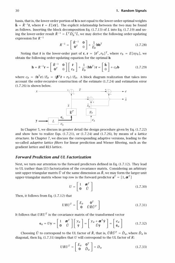
30 1. Random Signals
basis, that is, the lower-order portion of h is not equal to the lower-order optimal weightsh = R−1r, where r = E[xy]. The explicit relationship between the two may be foundas follows. Inserting the block decomposition Eq. (1.7.13) of L into Eq. (1.7.19) and us-ing the lower-order result R−1 = LTD−1
b L, we may derive the following order-updatingexpression for R−1
R−1 =[R−1 00T 0
]+ 1
EbbbT (1.7.28)
Noting that r is the lower-order part of r, r = [rT, rb]T, where rb = E[xyb], weobtain the following order-updating equation for the optimal h
h = R−1r =[R−1 00T 0
][rrb
]+ 1
Eb(bbT)r =
[h0
]+ cbb (1.7.29)
where cb = (bTr)/Eb = (βββT r + rb)/Eb. A block diagram realization that takes intoaccount the order-recursive construction of the estimate (1.7.24) and estimation error(1.7.26) is shown below.
In Chapter 5, we discuss in greater detail the design procedure given by Eq. (1.7.22)and show how to realize Eqs. (1.7.21), or (1.7.24) and (1.7.26), by means of a latticestructure. In Chapter 7, we discuss the corresponding adaptive versions, leading to theso-called adaptive lattice filters for linear prediction and Wiener filtering, such as thegradient lattice and RLS lattice.
Forward Prediction and UL Factorization
Next, we turn our attention to the forward predictors defined in Eq. (1.7.12). They leadto UL (rather than LU) factorization of the covariance matrix. Considering an arbitraryunit upper-triangular matrix U of the same dimension as R, we may form the larger unitupper-triangular matrix whose top row is the forward predictor aT = [1,αααT]
U =[
1 αααT
0 U
](1.7.30)
Then, it follows from Eq. (1.7.12) that
URUT =[Ea 0T
0 URUT
](1.7.31)
It follows that URUT is the covariance matrix of the transformed vector
ea = Uy =[
1 αααT
0 U
][yay
]=
[ya +αααTyUy
]=
[eaea
](1.7.32)
Choosing U to correspond to the UL factor of R, that is, URUT = Da, where Da isdiagonal, then Eq. (1.7.31) implies that U will correspond to the UL factor of R:
URUT =[Ea 0T
0 Da
]= Da (1.7.33)

1.7. Forward/Backward Prediction and LU/UL Factorization 31
This is equivalent to Eq. (1.6.14). The basis ea = Uy is completely decorrelated,with covariance matrix E[eaeTa]= Da. It is equivalent to Eq. (1.6.13). The rows of U arethe forward predictors of successive orders. And therefore, the UL factorization of Ris equivalent to performing the Gram-Schmidt construction starting at the endpoint yband proceeding to ya. The following example illustrates the method.
Example 1.7.2: By successively solving forward prediction problems of lower and lower order,construct the UL factorization of the covariance matrix R of Example 1.7.1.
Solution: Using Eq. (1.7.7), we find
ααα = −R−1ra = −[
3 22 3
]−1 [10
]= −1
5
[3 −2−2 3
][10
]=
[−3/5
2/5
]
Thus, aT = [1,αααT]= [1,−3/5,2/5]. The estimation error is
Ea = ρa +αααTra = 1+ [−3/5,2/5][
10
]= 2
5
Repeating the procedure on R =[
3 22 3
], we find the corresponding forward prediction
coefficients, satisfying Ra = Eau, where u =[
10
],
ααα = −[3]−1[2]= −2
3, aT = [1, αααT]= [1,−2/3]
and Ea = ρa + αααT ra = 3 − (2/3)×2 = 5/3. The rows of U are the forward predictorcoefficients and the diagonal entries of Da are the Eas:
U =⎡⎢⎣ 1 −3/5 2/5
0 1 −2/30 0 1
⎤⎥⎦ , Da =⎡⎢⎣ 2/5 0 0
0 5/3 00 0 3
⎤⎥⎦It is easily verified that URUT = Da. Note that the last entry of Da is always equal toρb. ��
Equation (1.7.33) can be used to compute the inverse of R:
R−1 = UTD−1a U (1.7.34)
Using the lower-order result R−1 = UTD−1a U and the decomposition (1.7.30), we find
the following order-updating equation for R−1, analogous to Eq. (1.7.28):
R−1 =[
0 0T
0 R−1
]+ 1
EaaaT (1.7.35)
Denoting r = E[xy] and ra = E[xya], we obtain the alternative order-update equa-tion for h, analogous to Eq. (1.7.29):
h = R−1r =[
0 0T
0 R−1
][rar
]+ 1
Ea(aTr)a =
[0h
]+ caa (1.7.36)
where ca = (aTr)/Ea = (ra + αααT r)/Ea, and h = R−1r is the lower-order optimalestimator for estimating x from y. By analogy with Eq. (1.7.21), we could also choose toexpress the estimates in the ea basis
x = hTy = hTU−1ea = gTuea (1.7.37)

32 1. Random Signals
where gu = U−Th. A realization is shown below.
The most important part of the realizations based on the diagonal bases ea or eais the preprocessing part that decorrelates the y basis, namely, eb = Ly, or ea = Uy.We will see in Chapters 5 and 7 that this part can be done efficiently using the Levinsonrecursion and the lattice structures of linear prediction. The LU representation, based onthe backward predictors, eb = Ly, is preferred because it is somewhat more convenientlyrealized in terms of the lattice structure than the UL representation ea = Uy.
Order Updates
So far, we studied the problems of forward and backward prediction separately fromeach other. Next, we would like to consider the two problems together and show how toconstruct the solution of the pair of equations (1.7.12) from the solution of a similar pairof lower order. This construction is the essence behind Levinson’s algorithm for solvingthe linear prediction problem, both in the stationary and in the adaptive least squarescases. Consider the following pair of lower-order forward and backward predictors,defined in terms of the block decompositions (1.7.5) of R:
Ra = Eau , Rb = Ebv (1.7.38)
where u and v are unit vectors of dimension one less than those of Eq. (1.7.12). Theyare related to u and v through the decompositions
u =[
u0
], v =
[0v
](1.7.39)
The basic result we would like to show is that the solution of the pair (1.7.12) maybe constructed from the solution of the pair (1.7.38) by
a =[
a0
]− γb
[0b
]
b =[
0b
]− γa
[a0
] (1.7.40)
This result is motivated by Eq. (1.7.39), which shows that the right-hand sides ofEqs. (1.7.38) are already part of the right-hand sides of Eq. (1.7.12), and therefore, thesolutions of Eq. (1.7.38) may appear as part of the solutions of (1.7.12). The predictionerrors are updated by
Ea = (1− γaγb)Ea , Eb = (1− γaγb)Eb (1.7.41)
where
γb = ΔaEb , γa = ΔbEa (1.7.42)
The γs are known as the reflection or PARCOR coefficients. The quantities Δa andΔb are defined by
Δa = aTrb , Δb = bT
ra (1.7.43)

1.7. Forward/Backward Prediction and LU/UL Factorization 33
The two Δs are equal, Δa = Δb, as seen from the following considerations. Usingthe decompositions (1.7.5), we find
R[
a0
]=
[R rbrTb ρb
][a0
]=
[RarTb a
]=
[EauΔa
]
R[
0b
]=
[ρa rTara R
][0b
]=
[rTa bRb
]=
[ΔbEbv
]They may be written more conveniently as
R[
a0
]=
[EauΔa
]= Ea
[u0
]+Δa
[01
]= Eau+Δav (1.7.44a)
R[
0b
]=
[ΔbEbv
]= Δb
[10
]+ Eb
[0v
]= Δbu+ Ebv (1.7.44b)
Noting that dTu and dTv are equal to the first and last components of a vector d, we
have [0, bT]u = 0 and [0, bT]v = 1 because the first and last components of [0, bT] arezero and one, respectively. Similarly, [aT,0]u = 1 and [aT,0]v = 0. Thus, multiplying
Eq. (1.7.44a) from the left by [0, bT] and Eq. (1.7.44b) by [aT,0], we find
[0, bT]R[
a0
]= Δa , [aT,0]R
[0b
]= Δb (1.7.45)
The equality of the Δs follows now from the fact that R is a symmetric matrix. Thus,
Δa = Δb ≡ Δ (1.7.46)
An alternative proof, based on partial correlations, will be given later. Equations(1.7.40) and (1.7.41) follow now in a straightforward fashion from Eq. (1.7.44). Multiply-ing the first part of Eq. (1.7.40) by R and using Eqs. (1.7.12) and (1.7.44), we find
Eau = Ra = R[
a0
]− γbR
[0b
]or,
Eau = (Eau+Δav)−γb(Δbu+ Ebv)= (Ea − γbΔb)u+ (Δb − γbEb)vwhich implies the conditions
Ea = Ea − γbΔb , Δa − γbEb = 0 (1.7.47)
Similarly, multiplying the second part of the Eq. (1.7.40) by R, we obtain
Ebv = (Δbu+ Ebv)−γa(Eau+Δbv)= (Δb − γaEa)u+ (Eb − γaΔa)vwhich implies
Eb = Eb − γaΔa , Δb − γaEa = 0 (1.7.48)
Equations (1.7.41) and (1.7.42) follow now from (1.7.47) and (1.7.48). By analogy withEq. (1.7.9), we may now define the prediction errors corresponding to the lower-orderpredictors a and b by
ea = aTy , eb = bT
y (1.7.49)
Using Eqs. (1.7.9) and (1.7.40), we find the following updating equations for the pre-diction errors
aTy = [aT,0][
yyb
]− γb[0, bT]
[yay
]= aTy− γbbTy
bTy = [0, bT][yay
]− γa[aT,0]
[yyb
]= b
Ty− γaaTy

34 1. Random Signals
or,ea = ea − γbeb , eb = eb − γaea (1.7.50)
A lattice type realization ofEq. (1.7.50) is shown below. It forms the basis of thelattice structures of linear prediction discussed in Chapters 5 and 7.
The order-updating procedure is illustrated by the following example.
Example 1.7.3: Using Eq. (1.7.40), construct the forward and backward predictors a and b foundpreviously in Examples 1.7.1 and 1.7.2.
Solution: The first part of Eq. (1.7.38), Ra = Eau is solved as follows:[1 11 3
][1α
]= Ea
[10
]⇒ α = −1
3, Ea = 2
3
Therefore, a =[
1−1/3
]. Similarly, Ry = Ebv, is solved by
[3 22 3
][β1
]= Eb
[01
]⇒ β = −2
3, Eb = 5
3
Hence, b =[−2/3
1
]. Next, we determine
Δ = aTrb = [1,−1/3][
02
]= −2
3, γb = Δ
Eb= −2
5, γa = Δ
Ea= −1
It follows from Eq. (1.7.40) that
a =[
a0
]− γb
[0b
]=
⎡⎢⎣ 1−1/3
0
⎤⎥⎦− (−2
5
)⎡⎢⎣ 0−2/3
1
⎤⎥⎦ =⎡⎢⎣ 1−3/52/5
⎤⎥⎦
b =[
0b
]− γa
[a0
]=
⎡⎢⎣ 0−2/3
1
⎤⎥⎦− (−1)
⎡⎢⎣ 1−1/3
0
⎤⎥⎦ =⎡⎢⎣ 1−11
⎤⎥⎦and the prediction errors are found from Eq. (1.7.41)
Ea = Ea(1− γaγb)= 2
3(1− 2/5)= 2
5, Eb = Eb(1− γaγb)= 5
3(1− 2/5)= 1
Partial Correlation Interpretation
Next, we show that γa and γb are partial correlation coefficients in the sense of Section1.6. Let yc denote all the components of y that lie between ya and yb, so that
y =⎡⎢⎣ yaycyb
⎤⎥⎦ , y =[yayc
], y =
[ycyb
](1.7.51)
The forward predictor a was defined as the best estimator of ya based on the restof the vector y. By the same token, a is the best estimator of ya based on the rest of y,

1.7. Forward/Backward Prediction and LU/UL Factorization 35
that is, yc. Similarly, the backward predictor b defines the best estimator of yb basedon the rest of the vector y; again, yc. Decomposing a and b as
a =[
1ααα
], b =
[βββ1
]we may write the best estimates of ya and yb based on yc as
ya/c = E[yayTc ]E[ycyTc ]−1yc = −αααTyc , yb/c = E[ybyTc ]E[ycyTc ]−1yc = −βββT
yc
and the estimation errors
ea = aTy = ya − ya/c , eb = bT
y = yb − yb/c (1.7.52)
Thus, ea and eb represent what is left of ya and yb after we project out their depen-dence on the intermediate vector yc. The direct influence of ya on yb, with the effectof yc removed, is measured by the correlation E[eaeb]. This correlation is equal to thequantity Δ defined in Eq. (1.7.46). This follows from Eq. (1.7.43)
Δa = aTrb = aTE[yby]= E[yb(aTy)
] = E[ybea]similarly,
Δb = bT
ra = bTE[yay]= E
[ya(b
Ty)
] = E[yaeb]Now, because ea is orthogonal to yc and yb/c is a linear combination of yc, it follows
that E[yb/cea]= 0. Similarly, because eb is orthogonal to yc and ya/c is linearly relatedto yc, it follows that E[ya/ceb]= 0. Thus,
Δa = E[ybea]= E[(yb − yb/c)ea]= E[ebea]
Δb = E[yaeb]= E[(ya − ya/c)eb]= E[eaeb]
Therefore, Δa and Δb are equal
Δa = Δb = E[eaeb] (1.7.53)
This is an alternative proof of Eq. (1.7.46). It follows that γa and γb are normalizedPARCOR coefficients in the sense of Section 1.6:
γb = E[eaeb]E[e2b]
, γa = E[ebea]E[e2a]
(1.7.54)
Using the Schwarz inequality for the inner product between two random variables,namely,
∣∣E[uv]∣∣2 ≤ E[u2]E[v2], we find the inequality
0 ≤ γaγb = E[eaeb]2
E[e2b]E[e
2a]≤ 1 (1.7.55)
This inequality also follows from Eq. (1.7.41) and the fact that Ea and Ea are positivequantities, both being mean square errors.
Example 1.7.4: For Example 1.7.1, compute the estimates ya/c and yb/c directly and comparethem with the results of Example 1.7.3.
Solution: From the matrix elements of R we have E[yayb]= 1, E[ybyc]= 2, and E[y2c]= 3.
Thus,
ya/c = E[yayc]E[y2c]−1yc = 1
3yc , yb/c = E[ybyc]E[y2
c]−1yc = 2
3yc
The corresponding errors will be
ea = ya − 1
3yc = [1,−1/3]y , eb = yb − 2
3yc = [−2/3,1]y
The results are identical to those of Example 1.7.3. ��

36 1. Random Signals
Conventional Cholesky Factorizations
Equation (1.7.18) shows that the conventional Cholesky factor ofR is given by the inversematrix L−1. A direct construction of the conventional Cholesky factor that avoids thecomputation of this inverse is as follows. Define
Gb = E[yeTb] (1.7.56)
If we use eb = Ly and E[ebeTb]= Db, it follows that
LGb = LE[yeTb]= E[ebeTb]= Dbor,
Gb = L−1Db (1.7.57)
Thus, Gb is a lower-triangular matrix. Its main diagonal consists of the diagonalentries of Db. Solving for L−1 = GbD−1
b and inserting in Eq. (1.7.18), we find the con-ventional LU factorization of R:
R = (GbD−1b )Db(D
−1b G
Tb)= GbD−1
b GTb (1.7.58)
Similarly, the conventional UL factorization of R is obtained from Eq. (1.7.33) bydefining the upper-triangular matrix
Ga = E[yeTa] (1.7.59)
Using ea = Uy and E[eaeTa]= Da, we find
UGa = Da ⇒ Ga = U−1Da (1.7.60)
which yields the conventional UL factorization of R:
R = U−1DaU−T = GaD−1a GTa
The columns of the matrices Ga and Gb will be referred to as the forward and back-ward gapped functions. This terminology will be justified in Chapters 2 and 5. Thedecomposition of Gb into its columns can be done order-recursively using the decom-position (1.7.15). We have
Gb = E[y[eTb , eb]
]≡ [Gb,gb] (1.7.61)
where Gb = E[yeTb] and gb = E[yeb]. Similarly, using Eq. (1.7.23) we find
Ga = E[y[ea, eTa]
] ≡ [ga, Ga] (1.7.62)
where Ga = E[yeTa] and ga = E[yea]. Motivated by the lattice recursions (1.7.50), weare led to define the lower-order gapped functions
gb = E[yeb] , ga = E[yea]
It follows that the gapped functions ga = E[yea] and gb = E[yeb] can be con-structed order-recursively by the lattice-type equations
ga = ga − γbgbgb = gb − γaga
(1.7.63)
The proof is straightforward. For example, E[yea]= E[y(ea − γbeb)
]. In Chapter
5 we will see that these equations are equivalent to the celebrated Schur algorithm for

1.7. Forward/Backward Prediction and LU/UL Factorization 37
solving the linear prediction problem. In recent years, the Schur algorithm has emergedas an important signal processing tool because it admits efficient fixed-point and parallelprocessor implementations. Equations (1.7.63) are mathematically equivalent to theLevinson-type recursions (1.7.40). In fact, Eq. (1.7.40) can be derived from Eq. (1.7.63)as follows. Using ea = aTy and eb = bTy, it follows that
ga = E[yea]= E[y(yTa)
] = Ra , gb = E[yeb]= E[y(yTb)
] = Rb
Similarly, we have
ga = R[
a0
], gb = R
[0b
](1.7.64)
These are easily shown. For example,
R[
a0
]= E[
y[yT, yb]][
a0
]= E[yyT]a = E[yea]= ga
Therefore, the first part of Eq. (1.7.63) is equivalent to
Ra = R[
a0
]− γbR
[0b
]Equation (1.7.40) follows now by canceling out the matrix factor R. One of the es-
sential features of the Schur algorithm is that the reflection coefficients can also becomputed from the knowledge of the lower-order gapped functions ga and gb, as fol-lows. Using Eq. (1.7.64) and dotting Eq. (1.7.44) with the unit vectors u and v, we find
Ea = uTga , Eb = vTgb , Δ = uTgb = vTga (1.7.65)
Thus, Eq. (1.7.42) may be written as
γb = vTgavTgb
, γb = uTgbuTga
(1.7.66)
Summary
We have argued that the solution of the general linear estimation problem can be mademore efficient by working with the decorrelated bases ea or eb, which contain no re-dundancies. Linear prediction ideas come into play in this context because the lineartransformations U and L that decorrelate the data vector y are constructible from theforward and backward linear prediction coefficients a and b. Moreover, linear predic-tion was seen to be equivalent to the Gram-Schmidt construction and to the Choleskyfactorization of the covariance matrix R. The order-recursive solutions of the linear pre-diction problem and the linear estimation problem, Eqs. (1.7.24) through (1.7.26), giverise to efficient lattice implementations with many desirable properties, such as robust-ness under coefficient quantization and modularity of structure admitting parallel VLSIimplementations.
In this section, we intentionally did not make any additional assumptions aboutany structural properties of the covariance matrix R. To close the loop and obtain theefficient computational algorithms mentioned previously, we need to make additionalassumptions on R. The simplest case is to assume that R has a Toeplitz structure. Thiscase arises when y is a block of successive signal samples from a stationary time series.The Toeplitz property means that the matrix elements along each diagonal of R are thesame. Equivalently, the matrix elementRij depends only on the difference of the indices,that is, Rij = R(i − j). With respect to the subblock decomposition (1.7.5), it is easilyverified that a necessary and sufficient condition for R to be Toeplitz is that
R = R

38 1. Random Signals
This condition implies that the linear prediction solutions for R and R must be thesame, that is,
b = b , a = a
Thus, from the forward and backward linear prediction solutions a and b of thelower-order Toeplitz submatrix R, we first obtain b = b and then use Eq. (1.7.40) to getthe linear prediction solution of the higher order matrix R. This is the essence behindLevinson’s algorithm. It will be discussed further in Chapters 2 and 5.
In the nonstationary time series case, the matrixR is not Toeplitz. Even then one canobtain some useful results by means of the so-called shift-invariance property. In thiscase, the data vector y consists of successive signal samples starting at some arbitrarysampling instant n
y(n)=
⎡⎢⎢⎢⎢⎢⎢⎢⎣
ynyn−1
...yn−M+1
yn−M
⎤⎥⎥⎥⎥⎥⎥⎥⎦ =[
y(n)yn−M
]=
[yn
y(n)
]
It follows that
y(n)=
⎡⎢⎢⎣yn...
yn−M+1
⎤⎥⎥⎦ , y(n)=
⎡⎢⎢⎣yn−1
...yn−M
⎤⎥⎥⎦ , or, y(n)= y(n− 1)
This implies that R(n)= R(n− 1), and therefore
a(n)= a(n− 1) , b(n)= b(n− 1)
Thus, order updating is coupled with time updating. These results are used in thedevelopment of the fast recursive least-squares adaptive filters, discussed in Chapter 7.
1.8 Random Signals
A random signal (random process, or stochastic process) is defined as a sequence ofrandom variables {x0, x1, x2, . . . , xn, . . . } where the index n is taken to be the time. Thestatistical description of so many random variables is very complicated since it requiresknowledge of all the joint densities
p(x0, x1, x2, . . . , xn) , for n = 0,1,2, . . .
If the mean E[xn] of the random signal is not zero, it can be removed by redefininga new signal xn − E[xn]. From now on, we will assume that this has been done, andshall work with zero-mean random signals. The autocorrelation function is defined as
Rxx(n,m)= E[xnxm] , n,m = 0,1,2, . . .
Sometimes it will be convenient to think of the random signal as a (possibly infinite)random vector x = [x0, x1, x2, . . . , xn, . . . ]T, and of the autocorrelation function as a(possibly infinite) matrix Rxx = E[xxT]. Rxx is positive semi-definite and symmetric.The autocorrelation function may also be written as
Rxx(n+ k,n)= E[xn+kxn] (1.8.1)

1.8. Random Signals 39
It provides a measure of the influence of the sample xn on the sample xn+k, whichlies in the future (if k > 0) by k units of time. The relative time separation k of the twosamples is called the lag.
If the signal xn is stationary (or wide-sense stationary), then the above average isindependent of the absolute time n, and is a function only of the relative lag k; abusingsomewhat the above notation, we may write in the case:
Rxx(k)= E[xn+kxn]= E[xn′+kxn′] (autocorrelation) (1.8.2)
In other words, the self-correlation properties of a stationary signal xn are sameon the average, regardless of when this average is computed. In a way, the stationaryrandom signal xn looks the same for all times. In this sense, if we take two differentblocks of data of lengthN, as shown in Fig. 1.4, we should expect the average properties,such as means and autocorrelations, extracted from these blocks of data to be roughlythe same. The relative time separation of the two blocks as a whole should not matter.
Fig. 1.4 Blocks of data from a stationary signal.
A direct consequence of stationarity is the reflection-invariance of the autocorrela-tion function Rxx(k) of Eq. (1.8.2):
Rxx(k)= E[xn+kxn]= Rxx(−k) (1.8.3)
One way to introduce a systematization of the various types of random signals isthe Markov classification into zeroth-order Markov, first-order Markov, and so on. Thesimplest possible random signal is the zeroth-order Markov, or purely random signal,defined by the requirement that all the (zero-mean) random variables xn be independentof each other and arise from a common density p(x); this implies
p(x0, x1,x2, . . . , xn)= p(x0)p(x1)p(x2)· · ·p(xn)· · ·Rxx(n,m)= E[xnxm]= 0 , for n =m
Such a random signal is stationary. The quantity Rxx(n,n) is independent of n, andrepresents the variance of each sample:
Rxx(0)= E[x2n]= σ2
x
In this case, the autocorrelation function Rxx(k) may be expressed compactly as
Rxx(k)= E[xn+kxn]= σ2xδ(k) (1.8.4)
A purely random signal has no memory, as can be seen from the property
p(xn, xn−1)= p(xn)p(xn−1) or, p(xn|xn−1)= p(xn)
that is, the occurrence of xn−1 at time instant n − 1 does not in any way affect, orrestrict, the values of xn at the next time instant. Successive signal values are entirelyindependent of each other. Past values do not influence future values. No memory is

40 1. Random Signals
retained from sample to sample; the next sample will take a value regardless of thevalue that the previous sample has already taken. Since successive samples are random,such a signal will exhibit very rapid time variations. But it will also exhibit slow timevariations. Such time variations are best discussed in the frequency domain. This willlead directly to frequency concepts, power spectra, periodograms, and the like. It isexpected that a purely random signal will contain all frequencies, from the very low tothe very high, in equal proportions (white noise).
The next least complicated signal is the first-order Markov signal, which has memoryonly of one sampling instant. Such a signal remembers only the previous sample. It isdefined by the requirement that
p(xn|xn−1, xn−1, . . . , x0)= p(xn|xn−1)
which states that xn may be influenced directly only by the previous sample value xn−1,and not by the samples xn−2, . . . , x0 that are further in the past. The complete statisticaldescription of such random signal is considerably simplified. It is sufficient to knowonly the marginal densities p(xn) and the conditional densities p(xn|xn−1). Any otherjoint density may be constructed in terms of these. For instance,
p(x3, x2, x1, x0) = p(x3|x2, x1, x0)p(x2, x1, x0) (by Bayes’ rule)
= p(x3|x2)p(x2, x1, x0) (by the Markov property)
= p(x3|x2)p(x2|x1, x0)p(x1, x0)
= p(x3|x2)p(x2|x1)p(x1, x0)
= p(x3|x2)p(x2|x1)p(x1|x0)p(x0)
1.9 Power Spectrum and Its Interpretation
The power spectral density of a stationary random signal xn is defined as the double-sided z-transform of its autocorrelation function
Sxx(z)=∞∑
k=−∞Rxx(k)z−k (1.9.1)
whereRxx(k)is given by Eq. (1.8.2). IfRxx(k) is strictly stable, the region of convergenceof Sxx(z) will include the unit circle in the complex z-plane. This allows us to definethe power spectrum Sxx(ω) of the random signal xn by setting z = ejω in Eq. (1.9.1).Abusing the notation somewhat, we have in this case
Sxx(ω)=∞∑
k=−∞Rxx(k)e−jωk (1.9.2)
This quantity conveys very useful information. It is a measure of the frequencycontent of the signal xn and of the distribution of the power of xn over frequency. Tosee this, consider the inverse z-transform
Rxx(k)=∮
u.c.Sxx(z)zk
dz2πjz
(1.9.3)
where, since Rxx(k) is stable, the integration contour may be taken to be the unit circle.Using z = ejω, we find for the integration measure
dz2πjz
= dω2π

1.9. Power Spectrum and Its Interpretation 41
Thus, Eq. (1.9.3) may also be written as an inverse Fourier transform
Rxx(k)=∫ π−πSxx(ω)ejωk
dω2π
(1.9.4)
In particular, the variance of xn can be written as
Rxx(0)= σ2x = E[x2
n]=∫ π−πSxx(ω)
dω2π
(1.9.5)
Since the quantity E[x2n] represents the average total power contained in xn, it fol-
lows that Sxx(ω) will represent the power per unit frequency interval. A typical powerspectrum is depicted in Fig. 1.5. As suggested by this figure, it is possible for the powerto be mostly concentrated about some frequencies and not about others. The area underthe curve represents the total power of the signal xn.
Fig. 1.5 Typical power spectrum.
If xn is an uncorrelated (white-noise) random signal with a delta-function autocorre-lation, given by Eq. (1.8.4), it will have a flat power spectrum with power level equal tothe variance σ2
x :
Sxx(ω)= σ2x
Another useful concept is that of the cross-correlation and cross-spectrum betweentwo stationary random sequences xn and yn. These are defined by
Ryx(k)= E[yn+kxn] , Syx(z)=∞∑
k=−∞Ryx(k)z−k (1.9.6)
Using stationarity, it is easy to show the reflection symmetry property
Ryx(k)= Rxy(−k) (1.9.7)
that is analogous to Eq. (1.8.3). In the z-domain, the reflection symmetry properties(1.8.3) and (1.9.7) are translated into:
Sxx(z)= Sxx(z−1) , Syx(z)= Sxy(z−1) (1.9.8)
respectively; and also
Sxx(ω)= Sxx(−ω) , Syx(ω)= Sxy(−ω) (1.9.9)

42 1. Random Signals
1.10 Sample Autocorrelation and the Periodogram
From now on we will work mostly with stationary random signals. If a block ofN signalsamples is available, we will assume that it is a segment from a stationary signal. Thelength N of the available data segment is an important consideration. For example, incomputing frequency spectra, we know that high resolution in frequency requires a longrecord of data. However, if the record is too long the assumption of stationarity may nolonger be justified. This is the case in many applications, as for example in speech andEEG signal processing. The speech waveform does not remain stationary for long timeintervals. It may be assumed to be stationary only for short time intervals. Such a signalmay be called piece-wise stationary. If it is divided into short segments of duration ofapproximately 20–30 milliseconds, then the portion of speech within each segment maybe assumed to be a segment from a stationary signal. A typical piece-wise stationarysignal is depicted in Fig. 1.6.
Fig. 1.6 Piece-wise stationary signal.
The main reason for assuming stationarity, or piece-wise stationarity, is that mostof our methods of handling random signals depend heavily on this assumption. Forexample, the statistical autocorrelations based on the ensemble averages (1.8.2) maybe replaced in practice by time averages. This can be justified only if the signals arestationary (actually, they must be ergodic). If the underlying signal processes are notstationary (and therefore definitely are not ergodic) we cannot use time averages. If asignal is piece-wise stationary and divided into stationary blocks, then for each suchblock, ensemble averages may be replaced by time averages. The time average approxi-mation of an autocorrelation function is called the sample autocorrelation and is definedas follows: Given a block of length N of measured signal samples
y0, y1, y2, . . . , yN−1
define
Ryy(k)= 1
N
N−1−k∑n=0
yn+kyn , for 0 ≤ k ≤ N − 1 (1.10.1)
andRyy(k)= Ryy(−k) , for − (N − 1)≤ k ≤ −1
The subroutine corr (see Appendix B) takes as inputs two length-N signal blocksyn, xn, n = 0,1, . . . ,N − 1, and computes their sample cross-correlation defined as
Ryx(k)= 1
N
N−1−k∑k=0
yn+kxn , k = 0,1, . . . ,N − 1
This routine may be used to compute either auto-correlations or cross-correlations.The periodogram is defined as the (double-sided) z-transform of the sample autocorre-lation
Syy(z)=N−1∑
k=−(N−1)Ryy(k)z−k (1.10.2)

1.10. Sample Autocorrelation and the Periodogram 43
It may be thought of as an approximation (estimate) of the true power spectral den-sity Syy(z). It is easily shown that the periodogram may be expressed in terms of thez-transform of the data sequence itself, as
Syy(z)= 1
NY(z)Y(z−1) (1.10.3)
where
Y(z)=N−1∑n=0
ynz−n (1.10.4)
As a concrete example, consider a length-3 signal y = [y0, y1, y2]T. Then,
Y(z)Y(z−1) = (y0 + y1z−1 + y2z−2)(y0 + y1z+ y2z2)
= (y20 + y2
1 + y22)+(y0y1 + y1y2)(z−1 + z)+(y0y2)(z−2 + z2)
from which we extract the inverse z-transform
Rxx(0) = 1
3(y2
0 + y21 + y2
2)
Rxx(−1)= Rxx(1) = 1
3(y0y1 + y1y2)
Rxx(−2)= Rxx(2) = 1
3(y0y2)
These equations may also be written in a nice matrix form, as follows
⎡⎢⎣ Rxx(0) Rxx(1) Rxx(2)Rxx(1) Rxx(0) Rxx(1)Rxx(2) Rxx(1) Rxx(0)
⎤⎥⎦︸ ︷︷ ︸
Ryy
= 1
3
⎡⎢⎣ y0 y1 y2 0 00 y0 y1 y2 00 0 y0 y1 y2
⎤⎥⎦︸ ︷︷ ︸
YT
⎡⎢⎢⎢⎢⎢⎢⎣y0 0 0y1 y0 0y2 y1 y0
0 y2 y1
0 0 y2
⎤⎥⎥⎥⎥⎥⎥⎦︸ ︷︷ ︸
Y
or,
Ryy = 1
3YTY
The matrix Ryy on the left is called the sample autocorrelation matrix. It is a Toeplitzmatrix, that is, it has the same entry in each diagonal. The right hand side also showsthat the autocorrelation matrix is positive definite. In the general case of a length-Nsequence yn, the matrix Y has N columns, each a down-shifted (delayed) version of theprevious one, corresponding to a total of N− 1 delays. This requires the length of eachcolumn to be N + (N − 1), that is, there are 2N − 1 rows. We will encounter again thismatrix factorization in the least-squares design of waveshaping filters.
The sample autocorrelation may also be thought of as ordinary convolution. Notethat Y(z−1) represents the z-transform the original signal y = [y0, y1, . . . , yN−1]T re-flected about the time origin. The reflected signal may be made causal by a delay ofN − 1 units of time. The reflected-delayed signal has some significance, and is knownas the reversed signal. Its z-transform is the reverse polynomial of Y(z)
YR(z)= z−(N−1)Y(z−1)
[ 0 0 · · · 0 y0 y1 · · · yN−2 yN−1 ] = original[ yN−1 yN−2 · · · y1 y0 0 · · · 0 0 ] = reflected[ 0 0 · · · 0 yN−1 yN−2 · · · y1 y0 ] = reversed

44 1. Random Signals
The periodogram is expressed then in the form
Sxx(z)= 1
NY(z)Y(z−1)= 1
NY(z)YR(z)zN−1
which implies that Ryy(k) may be obtained by convolving the original data sequencewith the reversed sequence and then advancing the result in time by N − 1 time units.This is seen by the following convolution table.
The periodogram spectrum is obtained by substituting z = ejω
Syy(ω)= 1
N∣∣Y(ω)∣∣2 = 1
N
∣∣∣∣∣∣N−1∑n=0
yne−jωn∣∣∣∣∣∣
2
(1.10.5)
The periodogram spectrum (1.10.5) may be computed efficiently using FFT methods.The digital frequencyω in units of [radians/sample] is related to the physical frequencyf in [Hz] by
ω = 2πfT = 2πffs
where fs is the sampling rate, and T = 1/fs, the time interval between samples. Thefrequency resolution afforded by a length-N sequence is
Δω = 2πN, or, Δf = fs
N= 1
NT= 1
TR[Hz]
where TR = NT is the duration of the data record in seconds. The periodogram spec-trum suffers from two major drawbacks. First, the rectangular windowing of the datasegment introduces significant sidelobe leakage. This can cause misinterpretation ofsidelobe spectral peaks as being part of the true spectrum. And second, it is well-knownthat the periodogram spectrum is not a good (consistent) estimator of the true powerspectrum Syy(ω).
The development of methods to improve on the periodogram is the subject of clas-sical spectral analysis [9–19]. We just mention, in passing, one of the most popular ofsuch methods, namely, Welch’s method [20]. The given data record of lengthN is subdi-vided intoK shorter segments which may be overlapping or non-overlapping. If they arenon-overlapping then each will have lengthM = N/K; if they are 50% overlapping thenM = 2N/(K + 1). Each such segment is then windowed by a length-M data window,such as a Hamming window. The window reduces the sidelobe frequency leakage at theexpense of resolution. The window w(n) is typically normalized to have unit averageenergy, that is, (1/M)
∑M−1n=0 w2(n)= 1. The periodogram of each windowed segment is
then computed by FFT methods and theK periodograms are averaged together to obtainthe spectrum estimate
S(ω)= 1
K
K∑i=1
Si(ω)
where Si(ω) is the periodogram of the ith segment. The above subdivision into seg-ments imitates ensemble averaging, and therefore, it results in a spectrum estimate ofimproved statistical stability. However, since each periodogram is computed from alength-M sequence, the frequency resolution is reduced from Δω = 2π/N to roughly

1.11. Random Signal Models and Their Uses 45
Δω = 2π/M (for a well-designed window). Therefore, to maintain high frequency reso-lution (largeM), as well as improved statistical stability of the spectrum estimate (largeK), a long data record N = MK is required—a condition that can easily come into con-flict with stationarity. The so-called “modern methods” of spectrum estimation, whichare based on parametric signal models, can provide high resolution spectrum estimatesfrom short data records.
1.11 Random Signal Models and Their Uses
Models that provide a characterization of the properties and nature of random signalsare of primary importance in the design of optimum signal processing systems. Thissection offers an overview of such models and outlines their major applications. Manyof the ideas presented here will be developed in greater detail in later chapters.
One of the most useful ways to model a random signal [21] is to consider it asbeing the output of a causal and stable linear filter B(z) that is driven by a stationaryuncorrelated (white-noise) sequence εn,
B(z)=∞∑n=0
bnz−n
where Rεε(k)= E[εn+kεn]= σ2εδ(k). Assuming a causal input sequence εn, the output
random signal yn is obtained by convolving εn with the filter’s impulse response bn:
yn =n∑i=0
bn−iεi (1.11.1)
The stability of the filter B(z) is essential as it guarantees the stationarity of thesequence yn. This point will be discussed later on. By readjusting, if necessary, thevalue of σ2
ε we may assume that b0 = 1. Then Eq. (1.11.1) corresponds exactly to theGram-Schmidt form of Eqs. (1.5.15) and (1.5.16), where the matrix elements bni are givenin terms of the impulse response of the filter B(z):
bni = bn−i (1.11.2)
In this case, the structure of the matrix B is considerably simplified. Writing theconvolutional equation (1.11.1) in matrix form⎡⎢⎢⎢⎢⎢⎢⎣
y0
y1
y2
y3
y4
⎤⎥⎥⎥⎥⎥⎥⎦ =⎡⎢⎢⎢⎢⎢⎢⎣
1 0 0 0 0b1 1 0 0 0b2 b1 1 0 0b3 b2 b1 1 0b4 b3 b2 b1 1
⎤⎥⎥⎥⎥⎥⎥⎦
⎡⎢⎢⎢⎢⎢⎢⎣ε0
ε1
ε2
ε3
ε4
⎤⎥⎥⎥⎥⎥⎥⎦ (1.11.3)
we observe that the first column of B is the impulse response bn of the filter. Eachsubsequent column is a down-shifted (delayed) version of the previous one, and eachdiagonal has the same entry (i.e., B is a Toeplitz matrix). The lower-triangular nature ofB is equivalent to the assumed causality of the filter B(z).
Such signal models are quite general. In fact, there is a general theorem by Wold thatessentially guarantees the existence of such models for any stationary signal yn [22,23].Wold’s construction of B(z) is none other than the Gram-Schmidt construction of theorthogonalized basis εn. However, the practical usage of such models requires furtherthat the transfer function B(z) be rational, that is, the ratio of two polynomials in z−1.In this case, the I/O convolutional equation (1.11.1) is most conveniently expressed asa difference equation.

46 1. Random Signals
Example 1.11.1: Suppose
B(z)= 1+ c1z−1 + c2z−2
1+ d1z−1 + d2z−2(1.11.4)
Then Eq. (1.11.1) is equivalent to the difference equation
yn = −d1yn−1 − d2yn−2 + εn + c1εn−1 + c2εn−2 (1.11.5)
which may be realized as follows
The filter B(z) is called a synthesis filter and may be thought of as a random signalgenerator, or a signal model, for the random signal yn. The numerator and denominatorcoefficients of the filter B(z), and the variance σ2
ε of the input white noise, are referredto as the model parameters. For instance, in Example 1.11.1 the model parameters are{c1, c2, d1, d2, σ2
ε}.Such parametric models have received a lot of attention in recent years. They are
very common in speech and geophysical signal processing, image processing, EEG sig-nal processing, spectrum estimation, data compression, and other time series analysisapplications.
How are such models used? One of the main objectives in such applications hasbeen to develop appropriate analysis procedures for extracting the model parameterson the basis of a given set of samples of the signal yn. This is a system identificationproblem. The analysis procedures are designed to provide effectively the best fit of thedata samples to a particular model. The procedures typically begin with a measuredblock of signal samples {y0, y1, . . . , yN}—also referred to as an analysis frame—andthrough an appropriate analysis algorithm extract estimates of the model parameters.This is depicted in Fig. 1.7.
Fig. 1.7 Analysis procedure.
The given frame of samples {y0, y1, . . . , yN} is represented now by the set of modelparameters extracted from it. Following the analysis procedure, the resulting modelmay be used in a variety of ways. The four major uses of such models are in:
1. Signal synthesis2. Spectrum estimation3. Signal classification4. Data compression
We will discuss each of these briefly. To synthesize a particular realization of therandom signal yn, it is only necessary to recall from memory the appropriate modelparameters, generate a random uncorrelated sequence εn having variance σ2
ε , and sendit through the filterB(z). Such uncorrelated sequence may be computer-generated usinga standard random number generator routine. The synthetic signal will appear at theoutput of the filter. This is shown in Fig. 1.8.

1.11. Random Signal Models and Their Uses 47
Fig. 1.8 Signal synthesis.
This is the basic principle behind most speech synthesis systems. In speech, thesynthesis filter B(z) represents a model of the transfer characteristics of the vocal tractconsidered as an acoustic tube. A typical analysis frame of speech has duration of20 msec. If sampled at a 10-kHz sampling rate, it will consist of N = 200 samples.To synthesize a particular frame of 200 samples, the model parameters representingthat frame are recalled from memory, and the synthesis filter is run for 200 samplinginstances generating 200 output speech samples, which may be sent to a D/A converter.The next frame of 200 samples can be synthesized by recalling from memory its modelparameters, and so on. Entire words or sentences can be synthesized in such a piece-wise, or frame-wise, manner.
A realistic representation of each speech frame requires the specification of twoadditional parameters besides the filter coefficients and σ2
ε , namely, the pitch periodand a voiced/unvoiced (V/UV) decision. Unvoiced sounds, such as the “sh” in the word“should”, have a white-noise sounding nature, and are generated by the turbulent flowof air through constrictions of the vocal tract. Such sounds may be represented ade-quately by the above random signal models. On the other hand, voiced sounds, such asvowels, are pitched sounds, and have a pitch period associated with them. They may beassumed to be generated by the periodic excitation of the vocal tract by a train of im-pulses separated by the pitch period. The vocal tract responds to each of these impulsesby producing its impulse response, resulting therefore in a quasi-periodic output whichis characteristic of such sounds. Thus, depending on the type of sound, the nature ofthe generator of the excitation input to the synthesis filter will be different, namely, itwill be a random noise generator for unvoiced sounds, and a pulse train generator forvoiced sounds. A typical speech synthesis system that incorporates the above featuresis shown in Fig. 1.9.
Fig. 1.9 Typical speech synthesis system.
Another major application of parametric models is to spectrum estimation. This isbased on the property that
Syy(ω)= σ2ε∣∣B(ω)∣∣2
(1.11.6)
which will be proved later. It states that the spectral shape of the power spectrumSyy(ω) of the signal yn arises only from the spectral shape of the model filter B(ω).For example, the signal yn generated by the model of Example 1.11.1 will have
Syy(ω)= σ2ε
∣∣∣∣∣ 1+ c1e−jω + c2e−2jω
1+ d1e−jω + d2e−2jω
∣∣∣∣∣2

48 1. Random Signals
This approach to spectrum estimation is depicted in Fig. 1.10. The parametric ap-proach to spectrum estimation must be contrasted with the classical approach which isbased on direct computation of the Fourier transform of the available data record, thatis, the periodogram spectrum, or its improvements. The classical periodogram methodis shown in Fig. 1.11. As we mentioned in the previous section, spectrum estimatesbased on such parametric models tend to have much better frequency resolution prop-erties than the classical methods, especially when the length N of the available datarecord is short.
Fig. 1.10 Spectrum estimation with parametric models.
Fig. 1.11 Classical spectrum estimation.
In signal classification applications, such as speech recognition, speaker verification,or EEG pattern classification, the basic problem is to compare two available blocks ofdata samples and decide whether they belong to the same class or not. One of the twoblocks might be a prestored and preanalyzed reference template against which the otherblock is to be compared. Instead of comparing the data records sample by sample, whatare compared are the corresponding model parameters extracted from these blocks.In pattern recognition nomenclature, the vector of model parameters is the “featurevector.” The closeness of the two sets of model parameters to each other is decidedon the basis of an appropriate distance measure. We will discuss examples of distancemeasures for speech and EEG signals in Chapter 5. This approach to signal classificationis depicted in Fig. 1.12.
Fig. 1.12 Signal classification with parametric models.
Next, we discuss the application of such models to data compression. The signalsynthesis method described above is a form of data compression because instead ofsaving the N data samples yn as such, what are saved are the corresponding modelparameters which are typically much fewer in number than N. For example, in speechsynthesis systems a savings of about a factor of 20 in memory may be achieved withthis approach. Indeed, as we discussed above, a typical frame of speech consists of 200samples, whereas the number of model parameters typically needed to represent thisframe is about 10 to 15. The main limitation of this approach is that the reproductionof the original signal segment is not exact but depends on the particular realization ofthe computer-generated input sequence εn that drives the model. Speech synthesized

1.11. Random Signal Models and Their Uses 49
in such manner is still intelligible, but it has lost some of its naturalness. Such signalsynthesis methods are not necessarily as successful or appropriate in all applications.For example, in image processing, if one makes a parametric model of an image andattempts to “synthesize” it by driving the model with a computer-generated uncorrelatedsequence, the reproduced image will bear no resemblance to the original image.
For exact reproduction, both the model parameters and the entire sequence εn mustbe stored. This would still provide some form of data compression, as will be explainedbelow. Such an approach to data compression is widely used in digital data transmissionor digital data storage applications for all types of data, including speech and imagedata. The method may be described as follows: the given data record {y0, y1, . . . , yN−1}is subjected to an appropriate analysis algorithm to extract the model parameters, andthen the segment is filtered through the inverse filter,
A(z)= 1
B(z)(1.11.7)
to provide the sequence εn. The inverse filter A(z) is also known as the whiteningfilter, the prediction-error filter, or the analysis filter. The resulting sequence εn hasa compressed dynamic range relative to yn and therefore it requires fewer number ofbits for the representation of each sample εn. A quantitative measure for the datacompression gain is given by the ratio G = σ2
y/σ2ε , which is always greater than one.
This can be seen easily using Eqs. (1.11.6) and (1.9.5)
σ2y =
∫ π−πSyy(ω)
dω2π
= σ2ε
∫ π−π
∣∣B(ω)∣∣2 dω2π
= σ2ε
∞∑n=0
b2n
Since b0 = 1, we find
G = σ2y
σ2ε=
∞∑n=0
b2n = 1+ b2
1 + b22 + · · · (1.11.8)
The entire sequence εn and the model parameters are then transmitted over thedata link, or stored in memory. At the receiving end, the original sequence yn may bereconstructed exactly using the synthesis filter B(z) driven by εn. This approach todata compression is depicted in Fig. 1.13. Not shown in Fig. 1.13 are the quantizationand encoding operations that must be performed on εn in order to transmit it over thedigital channel. An example that properly takes into account the quantization effectswill be discussed in more detail in Chapter 2.
Fig. 1.13 Data compression.
Filtering the sequence yn through the inverse filter requires that A(z) be stable andcausal. If we write B(z) as the ratio of two polynomials
B(z)= N(z)D(z)
(1.11.9)
then the stability and causality of B(z) requires that the zeros of the polynomial D(z)lie inside the unit circle in the complex z-plane; whereas the stability and causality ofthe inverse A(z)= D(z)/N(z) requires the zeros of N(z) to be inside the unit circle.Thus, both the poles and the zeros of B(z) must be inside the unit circle. Such filters

50 1. Random Signals
are called minimal phase filters and will be discussed further in Chapter 3. When A(z)is stable and causal it may be expanded in the form
A(z)=∞∑n=0
anz−n = 1+ a1z−1 + a2z−2 + · · · (1.11.10)
and the I/O equation of Eq. (1.11.7) becomes
εn =n∑i=0
aiyn−i = yn + a1yn−1 + a2yn−2 + · · · (1.11.11)
for n = 0,1,2, . . . . It may be written in matrix form εεε = Ay as⎡⎢⎢⎢⎢⎢⎢⎣ε0
ε1
ε2
ε3
ε4
⎤⎥⎥⎥⎥⎥⎥⎦ =⎡⎢⎢⎢⎢⎢⎢⎣
1 0 0 0 0a1 1 0 0 0a2 a1 1 0 0a3 a2 a1 1 0a4 a3 a2 a1 1
⎤⎥⎥⎥⎥⎥⎥⎦
⎡⎢⎢⎢⎢⎢⎢⎣y0
y1
y2
y3
y4
⎤⎥⎥⎥⎥⎥⎥⎦Both this matrix form and Eq. (1.11.11) are recognized as special cases of Eqs. (1.6.1)
and (1.6.10). According to Eq. (1.6.11), the quantity
yn/n−1 = −[a1yn−1 + a2yn−2 + · · · + any0
](1.11.12)
is the projection of yn on the subspace spanned by Yn−1 = {yn−1, yn−2, . . . , y0}. There-fore, it represents the best linear estimate of yn on the basis of (all) its past values Yn−1,that is, yn/n−1 is the best prediction of yn from its (entire) past. Equation (1.11.11) givesthe corresponding prediction error εn = yn − yn/n−1. We note here an interesting con-nection between linear prediction concepts and signal modeling concepts [21–25], thatis, that the best linear predictor (1.11.12) determines the whitening filter A(z) which,in turn, determines the generator model B(z)= 1/A(z) of yn. In other words, solvingthe prediction problem also solves the modeling problem.
The above modeling approach to the representation of stationary time series, andits relationship to the Gram-Schmidt construction and linear prediction was initiate byWold and developed further by Kolmogorov [22,24].
The most general model filter B(z) given in Eq. (1.11.9) is called an autoregressivemoving average (ARMA), or a pole-zero model. Two special cases of interest are themoving average (MA), or all-zero models, and the autoregressive (AR), or all-pole models.The MA model has a nontrivial numerator only, B(z)= N(z), so that B(z) is a finitepolynomial:
B(z)= 1+ b1z−1 + b2z−2 + · · · + bMz−M (MA model)
The AR model has a nontrivial denominator only, B(z)= 1/D(z), so that its inverseA(z)= D(z) is a polynomial:
B(z) = 1
1+ a1z−1 + a2z−2 + · · · + aMz−M (AR model)
A(z) = 1+ a1z−1 + a2z−2 + · · · + aMz−M
Autoregressive models are the most widely used models, because the analysis algo-rithms for extracting the model parameters {a1, a2, . . . , aM;σ2
ε} are fairly simple. In thesequel, we will concentrate mainly on such models.

1.12. Filter Model of First Order Autoregressive Process 51
1.12 Filter Model of First Order Autoregressive Process
To gain some understanding of filter models of the above type, we consider a very simpleexample of a first-order recursive filter B(z) driven by a purely random sequence ofvariance σ2
ε :
B(z)= 1
1− az−1
This serves also as a simple model for generating a first order Markov signal. Thesignal yn is generated by the difference equation of the filter:
yn = ayn−1 + εn (1.12.1)
Let the probability of the nth sample εn be f(εn). We would like to show that
p(yn|yn−1, yn−2, . . . , y1, y0)= p(yn|yn−1)= f(εn)= f(yn − ayn−1)
which not only shows the Markov property of yn, but also how to compute the relatedconditional density. Perhaps the best way to see this is to start at n = 0:
y0 = ε0 (assuming zero initial conditions)
y1 = ay0 + ε1
y2 = ay1 + ε2 , etc.
To compute p(y2|y1, y0), suppose that y1 and y0 are both given. Since y1 is given,the third equation above shows that the randomness left in y2 arises from ε2 only. Thus,p(y2|y1)= f(ε2). From the first two equations it follows that specifying y0 and y1 isequivalent to specifying ε0 and ε1. Therefore, p(y2|y1, y0)= f(ε2|ε1, ε0)= f(ε2), thelast equation following from the purely random nature of the sequence εn. We haveshown that
p(y2|y1, y0)= p(y2|y1)= f(ε2)= f(y2 − ay1)
Using the results of Section 1.8, we also note
p(y2, y1, y0) = p(y2|y1)p(y1|y0)p(y0)
= f(ε2)f(ε1)f(ε0)
= f(y2 − ay1)f(y1 − ay0)f(y0)
The solution of the difference equation (1.12.1) is obtained by convolving the impulseresponse of the filter B(z)
bn = anu(n) , u(n)= unit step
with the input sequence εn as follows:
yn =n∑i=0
biεn−i =n∑i=0
aiεn−i (1.12.2)
for n = 0,1,2, . . . . This is the innovations representation of yn given by Eqs. (1.5.15),(1.5.16), and (1.11.1). In matrix form it reads:⎡⎢⎢⎢⎣
y0
y1
y2
y3
⎤⎥⎥⎥⎦ =⎡⎢⎢⎢⎣
1 0 0 0a 1 0 0a2 a 1 0a3 a2 a 1
⎤⎥⎥⎥⎦⎡⎢⎢⎢⎣ε0
ε1
ε2
ε3
⎤⎥⎥⎥⎦ (1.12.3)

52 1. Random Signals
The inverse equation, εεε = B−1y = Ay, is obtained by writing Eq. (1.12.1) as εn =yn − ayn−1. In matrix form, this reads⎡⎢⎢⎢⎣
ε0
ε1
ε2
ε3
⎤⎥⎥⎥⎦ =⎡⎢⎢⎢⎣
1 0 0 0−a 1 0 0
0 −a 1 00 0 −a 1
⎤⎥⎥⎥⎦⎡⎢⎢⎢⎣y0
y1
y2
y3
⎤⎥⎥⎥⎦ (1.12.4)
According to the discussion of Example 1.6.1, the partial correlation coefficientscan be read off from the first column of this matrix. We conclude, therefore, that allpartial correlation coefficients of order greater than two are zero. This property is inaccordance with our intuition about first order Markov processes; due to the recursivenature of Eq. (1.12.1) a given sample, say yn, will have an indirect influence on all futuresamples. However, the only direct influence is to the next sample.
Higher order autoregressive random signals can be generated by sending white noisethrough higher order filters. For example, the second-order difference equation
yn = a1yn−1 + a2yn−2 + εn (1.12.5)
will generate a second-order Markov signal. In this case, the difference equation di-rectly couples two successive samples, but not more than two. Therefore, all the partialcorrelations of order greater than three will be zero. This may be seen also by writingEq. (1.12.5) in matrix form and inspecting the first column of the matrix A:⎡⎢⎢⎢⎢⎢⎢⎣
ε0
ε1
ε2
ε3
ε4
⎤⎥⎥⎥⎥⎥⎥⎦ =⎡⎢⎢⎢⎢⎢⎢⎣
1 0 0 0 0−a1 1 0 0 0−a2 −a1 1 0 0
0 −a2 −a1 1 00 0 −a2 −a1 1
⎤⎥⎥⎥⎥⎥⎥⎦
⎡⎢⎢⎢⎢⎢⎢⎣y0
y1
y2
y3
y4
⎤⎥⎥⎥⎥⎥⎥⎦
1.13 Stability and Stationarity
In this section we discuss the importance of stability of the signal generator filter B(z).We demonstrate that the generated signal yn will be stationary only if the generatingfilter is stable. And in this case, the sequence yn will become stationary only after thetransient effects introduced by the filter have died out.
To demonstrate these ideas, consider the lag-0 autocorrelation of our first orderMarkov signal
Ryy(n,n) = E[y2n]= E
[(ayn−1 + εn)2]
= a2E[y2n−1]+2aE[yn−1εn]+E[ε2
n]= a2Ryy(n− 1, n− 1)+σ2ε
(1.13.1)
where we set σ2ε = E[ε2
n] and E[yn−1εn]= 0, which follows by using Eq. (1.12.2) to get
yn−1 = εn−1 + aεn−2 + · · · + an−1ε0
and noting that εn is uncorrelated with all these terms, due to its white-noise nature.The above difference equation for Ryy(n,n) can now be solved to get
Ryy(n,n)= E[y2n]=
σ2ε
1− a2+σ2
ε
(1− 1
1− a2
)a2n (1.13.2)
where the initial condition was taken to be E[y20]= E[ε2
0]= σ2ε . If the filter is stable and
causal, that is, |a| < 1, then the second term in (1.13.2) tends to zero exponentially, and
1.14. Parameter Estimation by the Maximum Likelihood Method 53
Ryy(n,n) eventually loses its dependence on the absolute time n. For large n, it tendsto the steady-state value
Ryy(0)= E[y2n]= σ2
y =σ2ε
1− a2(1.13.3)
The same result is obtained, of course, by assuming stationarity from the start. Thedifference equation (1.13.1) can be written as
E[y2n]= a2E[y2
n−1]+σ2ε
If yn is assumed to be already stationary, then E[y2n]= E[y2
n−1]. This implies thesame steady-state solution as Eq. (1.13.3).
If the filter is unstable, that is, |a| > 1, then the second term of Eq. (1.13.2) divergesexponentially. The marginal case a = 1 is also unacceptable, but is of historical interestbeing the famous Wiener process, or random walk. In this case, the signal model is
yn = yn−1 + εnand the difference equation for the variance becomes
Ryy(n,n)= Ryy(n− 1, n− 1)+σ2ε
with solutionRyy(n,n)= E[y2
n]= (n+ 1)σ2ε
In summary, for true stationarity to set in, the signal generator filter B(z) must bestrictly stable (all its poles must be strictly inside the unit circle).
1.14 Parameter Estimation by the Maximum Likelihood Method
One of the most important practical questions is how to extract the model parameters,such as the above filter parameter a, from the actual data values. As an introduction tothe analysis methods used to answer this question, let us suppose that the white noiseinput sequence εn is gaussian
f(εn)= 1√2πσε
exp(− ε2
n2σ2
ε
)and assume that a block of N measured values of the signal yn is available
y0, y1, y2, . . . , yN−1
Can we extract the filter parameter a from this block of data? Can we also extractthe variance σ2
ε of the driving white noise εn? If so, then instead of saving the N mea-sured values {y0, y1, y2, . . . , yN−1}, we can save the extracted filter parameter a and thevariance σ2
ε . Whenever we want to synthesize our original sequence yn, we will simplygenerate a white-noise input sequence εn of variance σ2
ε , using a pseudorandom num-ber generator routing, and then drive with it the signal model whose parameter a waspreviously extracted from the original data. Somehow, all the significant informationcontained in the original samples, has now been packed or compressed into the twonumbers a and σ2
ε .One possible criterion for extracting the filter parametera is the maximum likelihood
(ML) criterion: The parameter a is selected so as to maximize the joint density
p(y0, y1, . . . , yN−1)= f(ε0)f(ε1)· · · f(εN−1)
= 1(√2πσε
)N exp
⎡⎣− 1
2σ2ε
N−1∑n=1
(yn − ayn−1)2
⎤⎦ exp[−y2
0/2σ2ε]

54 1. Random Signals
that is, the parameter a is selected so as to render the actual measured values {y0, y1, y2,. . . , yN−1} most likely. The criterion is equivalent to minimizing the exponent withrespect to a:
E(a)=N−1∑n=1
(yn − ayn−1)2+y20 =
N−1∑n=0
e2n = min (1.14.1)
where we set en = yn − ayn−1, and e0 = y0. The minimization of Eq. (1.14.1) gives
∂E(a)∂a
= −2N−1∑n=1
(yn − ayn−1)yn−1 = 0 , or,
a =
N−1∑n=1
ynyn−1
N−1∑n−1
y2n−1
= y0y1 + y1y2 + · · · + yN−2yN−1
y20 + y2
1 + · · · + y2N−2
(1.14.2)
There is a potential problem with the above ML criterion for extracting the filterparameter a, namely, the parameter may turn out to have magnitude greater than one,which will correspond to an unstable filter generating the sequence yn. This is easilyseen from Eq. (1.14.2); whereas the numerator has dependence on the last sample yN−1,the denominator does not. Therefore it is possible, for sufficiently large values of yN−1,for the parameter a to be greater than one. There are other criteria for extracting theMarkov model parameters that guarantee the stability of the resulting synthesis filters,such as the so-called autocorrelation method, or Burg’s method. These will be discussedlater on.
1.15 Parameter Estimation by the Yule-Walker Method
In this section, we introduce the autocorrelation or Yule-Walker method of extracting themodel parameters from a block of data. We begin by expressing the model parametersin terms of output statistical quantities and then replace ensemble averages by timeaverages. Assuming stationarity has set in, we find
Ryy(1)= E[ynyn−1]= E[(ayn−1 + εn)yn−1
] = aE[y2n−1]+E[εnyn−1]= aRyy(0)
from which
a = Ryy(1)Ryy(0)
The input parameter σ2ε can be expressed as
σ2ε = (1− a2)σ2
y = (1− a2)Ryy(0)
These two equations may be written in matrix form as[Ryy(0) Ryy(1)Ryy(1) Ryy(0)
][1−a
]=
[σ2ε
0
]
These are called the normal equations of linear prediction. Their generalization willbe considered later on. These results are important because they allow the extractionof the signal model parameters directly in terms of output quantities, that is, fromexperimentally accessible quantities.
We may obtain estimates of the model parameters by replacing the theoretical auto-correlations by the corresponding sample autocorrelations, defined by Eq. (1.10.1):
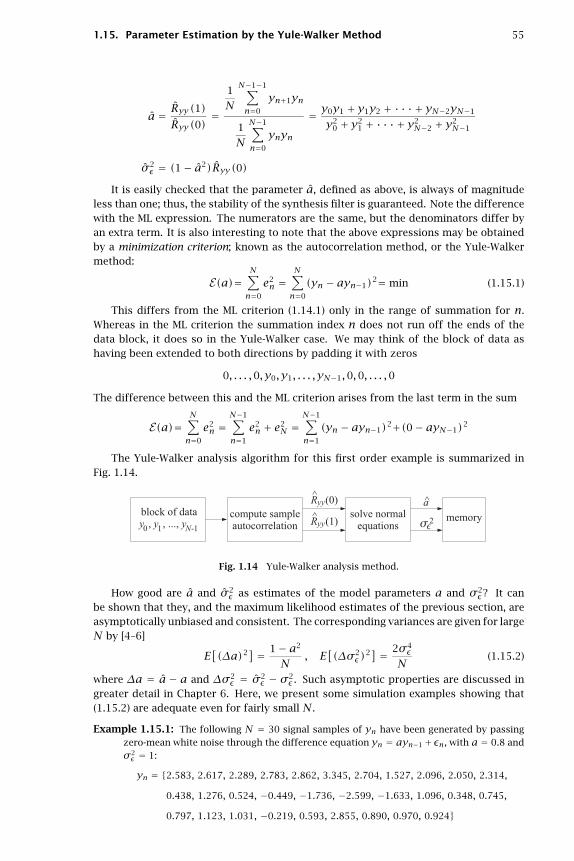
1.15. Parameter Estimation by the Yule-Walker Method 55
a = Ryy(1)Ryy(0)
=
1
N
N−1−1∑n=0
yn+1yn
1
N
N−1∑n=0
ynyn
= y0y1 + y1y2 + · · · + yN−2yN−1
y20 + y2
1 + · · · + y2N−2 + y2
N−1
σ2ε = (1− a2)Ryy(0)
It is easily checked that the parameter a, defined as above, is always of magnitudeless than one; thus, the stability of the synthesis filter is guaranteed. Note the differencewith the ML expression. The numerators are the same, but the denominators differ byan extra term. It is also interesting to note that the above expressions may be obtainedby a minimization criterion; known as the autocorrelation method, or the Yule-Walkermethod:
E(a)=N∑n=0
e2n =
N∑n=0
(yn − ayn−1)2= min (1.15.1)
This differs from the ML criterion (1.14.1) only in the range of summation for n.Whereas in the ML criterion the summation index n does not run off the ends of thedata block, it does so in the Yule-Walker case. We may think of the block of data ashaving been extended to both directions by padding it with zeros
0, . . . ,0, y0, y1, . . . , yN−1,0,0, . . . ,0
The difference between this and the ML criterion arises from the last term in the sum
E(a)=N∑n=0
e2n =
N−1∑n=1
e2n + e2
N =N−1∑n=1
(yn − ayn−1)2+(0− ayN−1)2
The Yule-Walker analysis algorithm for this first order example is summarized inFig. 1.14.
Fig. 1.14 Yule-Walker analysis method.
How good are a and σ2ε as estimates of the model parameters a and σ2
ε? It canbe shown that they, and the maximum likelihood estimates of the previous section, areasymptotically unbiased and consistent. The corresponding variances are given for largeN by [4–6]
E[(Δa)2] = 1− a2
N, E
[(Δσ2
ε)2] = 2σ4εN
(1.15.2)
where Δa = a − a and Δσ2ε = σ2
ε − σ2ε . Such asymptotic properties are discussed in
greater detail in Chapter 6. Here, we present some simulation examples showing that(1.15.2) are adequate even for fairly small N.
Example 1.15.1: The following N = 30 signal samples of yn have been generated by passingzero-mean white noise through the difference equation yn = ayn−1+εn, with a = 0.8 andσ2ε = 1:
yn = {2.583, 2.617, 2.289, 2.783, 2.862, 3.345, 2.704, 1.527, 2.096, 2.050, 2.314,
0.438, 1.276, 0.524, −0.449, −1.736, −2.599, −1.633, 1.096, 0.348, 0.745,
0.797, 1.123, 1.031, −0.219, 0.593, 2.855, 0.890, 0.970, 0.924}

56 1. Random Signals
Using the Yule-Walker method, we obtain the following estimates of the model parameters
a = 0.806 , σ2ε = 1.17
Both estimates are consistent with the theoretically expected fluctuations about their meansgiven by Eq. (1.15.2), falling within the one-standard deviation intervals a± δa and σ2
ε ±δσ2
ε , where δa and δσ2ε are the square roots of Eq. (1.15.2). For N = 30, the numerical
values of these intervals are: 0.690 ≤ a ≤ 0.910 and 0.742 ≤ σ2ε ≤ 1.258. Given the
theoretical and estimated model parameters, we can obtain the theoretical and estimatedpower spectral densities of yn by
STH(ω)= σ2ε∣∣1− ae−jω∣∣2 , SYW(ω)= σ2
ε∣∣1− ae−jω∣∣2
The periodogram spectrum based on the given length-N data block is
SPER(ω)= 1
N
∣∣∣∣∣∣N−1∑n=0
yne−jnω∣∣∣∣∣∣
2
The three spectra are plotted in Fig. 1.15, in units of decibels; that is, 10 log10 S, overthe right half of the Nyquist interval 0 ≤ ω ≤ π. Note the excellent agreement of theYule-Walker spectrum with the theoretical spectrum and the several sidelobes of the peri-odogram spectrum caused by the windowing of yn.
0 0.2 0.4 0.6 0.8 1−20
−10
0
10
20
digital frequency ω in units of π
dB
Yule−Walker vs. Periodogram Spectra
STH
SYW
Sper
Fig. 1.15 Comparison of Yule-Walker and periodogram spectrum estimates.
Example 1.15.2: The purpose of this example is to demonstrate the reasonableness of theasymptotic variances, Eq. (1.15.2). For the first-order model defined in the previous ex-ample, we generated 100 different realizations of the length-30 signal block yn. Fromeach realization, we extracted the Yule-Walker estimates of the model parameters a andσ2ε . They are shown in Figs. 1.16 and 1.17 versus realization index, together with the corre-
sponding asymptotic one-standard deviation intervals that were computed in the previousexample.
1.16 Linear Prediction and Signal Modeling
Linear prediction ideas are introduced in the context of our simple example by notingthat the least-squares minimization criteria (1.14.1) and (1.15.1)
E(a)=∑ne2n = minimum (1.16.1)

1.16. Linear Prediction and Signal Modeling 57
0 20 40 60 80 1000
0.4
0.8
1.2
realization index
a
Estimated Filter Parameter
0 20 40 60 80 1000
0.5
1
1.5
2
realization index
vari
ance
Estimated Input Variance
Fig. 1.16 and Fig. 1.17 Model parameters a,σ2ε estimated from 100 realizations of the length-30
data block yn.
essentially force each en to be small. Thus, if we reinterpret
yn = ayn−1
as the linear prediction of the sample yn made on the basis of just the previous sampleyn−1, then en = yn − ayn−1 = yn − yn may be thought of as the prediction error. Theminimization criterion (1.16.1) essentially minimizes the prediction error in an averageleast-squares sense, thus attempting to make the best prediction possible.
As we mentioned in Section 1.11, the solution of the linear prediction problem pro-vides the corresponding random signal generator model for yn, which can be used, inturn, in a number of ways as outlined in Section 1.11. This is the main reason for ourinterest in linear prediction.
A more intuitive way to understand the connection between linear prediction andsignal models is as follows: Suppose we have a predictor yn of yn which is not necessarilythe best predictor. The predictor yn is given as a linear combination of the past values{yn−1, yn−2, . . . }:
yn = −[a1yn−1 + a2yn−2 + · · ·
](1.16.2)
The corresponding prediction error will be
en = yn − yn = yn + a1yn−1 + a2yn−2 + · · · (1.16.3)
and it may be considered as the output of the prediction-error filter A(z) (which isassumed to be stable and causal):
A(z)= 1+ a1z−1 + a2z−2 + · · ·
Suppose further that A(z) has a stable and causal inverse filter
B(z)= 1
A(z)= 1
1+ a1z−1 + a2z−2 + · · ·so that yn may be expressed causally in terms of en, that is,
yn = en + b1en−1 + b2en−2 + · · · (1.16.4)
Then, Eqs. (1.16.3) and (1.16.4) imply that the linear spaces generated by the randomvariables
{yn−1, yn−2, . . . } and {en−1, en−2, . . . }

58 1. Random Signals
are the same space. One can pass from one set to the other by a causal and causallyinvertible linear filtering operation.
Now, if the prediction yn of yn is the best possible prediction, then what remains afterthe prediction is made—namely, the error signal en—should be entirely unpredictableon the basis of the past values {yn−1, yn−2, . . . }. That is, en must be uncorrelated withall of these. But this implies that en must be uncorrelated with all {en−1, en−2, . . . }, andtherefore en must be a white-noise sequence. It follows that A(z) and B(z) are theanalysis and synthesis filters for the sequence yn.
The least-squares minimization criteria of the type (1.16.1) that are based on timeaverages, provide a practical way to solve the linear prediction problem and hence alsothe modeling problem. Their generalization to higher order predictors will be discussedin Chapter 5.
1.17 Cramer–Rao Bound and Maximum Likelihood
The Cramer-Rao inequality [2–5,26] provides a lower bound for the variance of unbi-ased estimators of parameters. Thus, the best any parameter estimator can do is tomeet its Cramer-Rao bound. Such estimators are called efficient. Parameter estima-tors based on the principle of maximum likelihood, such as the one presented in Section1.14, have several nice properties, namely, as the number of observations becomes large,they are asymptotically unbiased, consistent, efficient, and are asymptotically normallydistributed about the theoretical value of the parameter with covariance given by theCramer-Rao bound.
In this section, we present a derivation of the Cramer-Rao inequality using correla-tion canceling methods and discuss its connection to maximum likelihood. ConsiderN observations Y = {y1,y2, . . . ,yN}, where each observation is assumed to be an M-dimensional random vector. Based on these observations, we would like to estimate anumber of (deterministic) parameters, assembled into a parameter vector λλλ. We willwrite p(Y,λλλ) to indicate the dependence of the joint probability density on λλλ. As aconcrete example, consider the case of N independent scalar observations drawn froma normal distribution with meanm and variance σ2. The joint density is
p(Y,λλλ)= (2πσ2)−N/2exp
⎡⎣− 1
2σ2
N∑n=1
(yn −m)2
⎤⎦ (1.17.1)
For the parameter vector we may choose λλλ = [m,σ2]T, if we want to estimate boththe mean and variance.
The dependence of p(Y,λλλ) on λλλ may be expressed in terms of the gradient withrespect to λλλ of the log-likelihood function
ψψψ(Y,λλλ)≡ ∂∂λλλ
lnp(Y,λλλ)= 1
p∂p∂λλλ
(1.17.2)
Expectation values with respect to the joint density will, in general, depend on theparameter λλλ. We have the following result for the expectation value of an arbitraryfunction F(Y,λλλ):
∂∂λλλE[F]= E
[∂F∂λλλ
]+ E[Fψψψ] (1.17.3)
Writing dY = dMy1dMy2 · · ·dMyN for the volume element over the space of obser-vations, the proof of Eq. (1.17.3) follows from
∂∂λλλ
∫pFdY =
∫∂∂λλλ(pF)dY =
∫p∂F∂λλλdY +
∫pF∂ lnp∂λλλ
dY

1.17. Cramer–Rao Bound and Maximum Likelihood 59
Applying this property to F = 1, we find E[ψψψ]= 0. Applying it to ψψψ itself, that is,F =ψψψ, we find
J ≡ E[ψψψψψψT]= E[Ψ] (1.17.4)
where
Ψ ≡ −∂ψψψ∂λλλ
Eq. (1.17.4) is known as the Fisher information matrix based on Y. Component-wise,we have
Jij = E[ψiψj]= E[Ψij]where
ψi = ∂ lnp∂λi
, Ψij = −∂ψi∂λj= − ∂
2 lnp∂λi∂λj
Next, we derive the Cramer-Rao bound. Let λλλ(Y) be any estimator of λλλ based on Y.Because λλλ(Y) andψψψ(Y,λλλ) both depend on Y, they will be correlated with each other.Using the correlation canceling methods of Section 1.4, we can remove these correlationsby writing
e = λλλ− E[λλλψψψT]E[ψψψψψψT]−1ψψψ
Then, e will not be correlated with ψψψ. Because ψψψ has zero mean, it follows thatE[λλλ]= E[e]. Working with the deviations about the corresponding means, namely,Δλλλ = λλλ− E[λλλ] and Δe = e− E[e], we have
Δe = Δλλλ−MJ−1ψψψ (1.17.5)
where we denoted M = E[λλλψψψT]. Following Eq. (1.4.4), we obtain for the covariance ofΔe
E[ΔeΔeT]= E[ΔλλλΔλλλT]−MJ−1MT (1.17.6)
Thus, the difference of terms in the right-hand side is a positive semi-definite matrix.This may be expressed symbolically as E[ΔeΔeT]≥ 0, or, E[ΔλλλΔλλλT]≥ MJ−1MT. Thequantity M depends on the bias of the estimator. For an unbiased estimator, M is theidentity matrix,M = I, and we obtain the Cramer-Rao inequality
cov(λλλ)= E[ΔλλλΔλλλT]≥ J−1 (Cramer-Rao) (1.17.7)
The dependence of M on the bias can be seen as follows. Because λλλ(Y) has noexplicit dependence on λλλ, it follows from property (1.17.3) that
M = E[λλλψψψT]= ∂∂λλλE[λλλ]
Define the bias of the estimator as the deviation of the mean from the true value ofthe parameter, that is, E[λλλ]= λλλ+ b(λλλ), where b(λλλ) is the bias
M = I + ∂b
∂λλλ≡ I + B
For an unbiased estimator, B = 0 and M = I. It follows from Eq. (1.17.6) that forthe Cramer-Rao inequality to be satisfied as an equality, it is necessary that Δe = 0in Eq. (1.17.5), i.e., Δλλλ = MJ−1ψψψ and in the unbiased case, we obtain the conditionψψψ = JΔλλλ:
∂∂λλλ
lnp(Y,λλλ)= JΔλλλ = J[λλλ(Y)−λλλ](1.17.8)
Estimators that satisfy this condition and thus, meet their Cramer-Rao bound, arecalled efficient.

60 1. Random Signals
Example 1.17.1: The log-likelihood function of Eq. (1.17.1) is
lnp = −N2
ln(2π)−N2
lnσ2 − 1
2σ2
N∑n=1
(yn −m)2
The gradients with respect to the parametersm and σ2 are
∂ lnp∂m
= 1
σ2
N∑n=1
(yn −m)
∂ lnp∂σ2
= − N2σ2
+ 1
2σ4
N∑n=1
(yn −m)2
(1.17.9)
The second derivatives are the matrix elements of the matrix Ψ:
Ψmm = − ∂2 lnp∂m∂m
= Nσ2
Ψmσ2 = − ∂2 lnp
∂m∂σ2= 1
σ4
N∑n=1
(yn −m)
Ψσ2σ2 = − ∂2 lnp∂σ2∂σ2
= − N2σ4
+ 1
σ6
N∑n=1
(yn −m)2
Taking expectation values, we find the matrix elements of J
Jmm = Nσ2, Jmσ2 = 0 , Jσ2σ2 = N
2σ4
Therefore, the Cramer-Rao bound of any unbiased estimator ofm and σ2 will be[E[ΔmΔm] E[ΔmΔσ2]E[Δσ2Δm] E[Δσ2Δσ2]
]≥
[σ2/N 0
0 2σ4/N
]
Example 1.17.2: We note that the sample mean m defined by Eq. (1.2.1) has variance equal toits Cramer-Rao bound, and therefore, it is an efficient estimator. It also satisfies condition(1.17.8). Writing
∑Nn=1 yn = Nm, we obtain from Eq. (1.17.9)
∂ lnp∂m
= 1
σ2
N∑n=1
(yn −m)= 1
σ2
⎡⎣ N∑n=1
yn −Nm⎤⎦ = 1
σ2(Nm−Nm)= Jmm(m−m)
We also note that the sample variance s2 having variance 2σ4/(N − 1) meets its Cramer-Rao bound only asymptotically. The biased definition of the sample variance, Eq. (1.2.3),has variance given by Eq. (1.2.4). It is easily verified that it is smaller than its Cramer-Raobound (1.17.7). But this is no contradiction because Eq. (1.17.7) is valid only for unbiasedestimators. For a biased estimator, the lower bound MJ−1MT must be used. Equation(1.2.4) does satisfy this bound. ��
Next, we discuss the principle of maximum likelihood. The maximum likelihoodestimator of a parameter λλλ is the value λλλ that maximizes the joint density p(Y,λλλ); i.e.,
p(Y,λλλ)∣∣λλλ=λλλ = maximum (1.17.10)
Equivalently,
ψψψ(λλλ)= ∂∂λλλ
lnp(Y,λλλ)∣∣∣∣λλλ=λλλ
= 0 (1.17.11)
In general, this equation is difficult to solve. However, the asymptotic properties ofthe solution for large N are simple enough to obtain. Assuming that λλλ is near the truevalue of the parameter λλλ we may expand the gradientψψψ about the true value:
ψψψ(λλλ)�ψψψ+ ∂ψψψ(λλλ)∂λλλ
(λλλ−λλλ)=ψψψ−Ψ(λλλ−λλλ)

1.17. Cramer–Rao Bound and Maximum Likelihood 61
where we used the matrixΨ defined in Eq. (1.17.4). For the maximum likelihood solution,the left-hand side is zero. Thus, solving for Δλλλ = λλλ−λλλ, we obtain
Δλλλ = Ψ−1ψψψ (1.17.12)
Assuming that the N observations are independent of each other, the joint densityp(Y,λλλ) factors into the marginal densities
∏Nn=1 p(yn,λλλ). Therefore, the gradient ψψψ
will be a sum of gradients
ψψψ = ∂∂λλλ
lnp =N∑n=1
∂∂λλλ
lnp(yn,λλλ)=N∑n=1
ψψψn
Similarly,
Ψ = −∂ψψψ∂λλλ−
N∑n=1
∂ψψψn∂λλλ
=N∑N=1
Ψn
Individual terms in these sums are mutually independent. Thus, from the law oflarge numbers, we can replace Ψ by its mean Ψ � E[Ψ]= J, and Eq. (1.17.12) becomes
Δλλλ = J−1ψψψ (1.17.13)
This asymptotic equation contains essentially all the nice properties of the maxi-mum likelihood estimator. First, from E[Ψ]= 0, it follows that E[Δλλλ]= 0, or that λλλ isasymptotically unbiased. Second, its asymptotic covariance agrees with the Cramer-Raobound
E[ΔλλλΔλλλT]= J−1E[ψψψψψψT]J−1 = J−1JJ−1 = J−1
Thus, λλλ is asymptotically efficient. The same conclusion can be reached by notingthat Eq. (1.17.13) is the same as condition (1.17.8). Third, λλλ is asymptotically consistent,in the sense that its covariance tends to zero for large N. This follows from the factthat the information matrix for N independent observations is equal to N times theinformation matrix for one observation:
J = E[Ψ]=N∑n=1
E[Ψn]= NE[Ψ1]= NJ1
Therefore, J−1 = J−11 /N tends to zero for large N. Fourth, because ψψψ is the sum
of N independent terms, it follows from the vector version of the central limit theoremthatψψψ will be asymptotically normally distributed. Thus, so will be λλλ, with mean λλλ andcovariance J−1.
Example 1.17.3: Setting the gradients (1.17.9) to zero, we obtain the maximum likelihood esti-mates of the parametersm and σ2. It is easily verified that they coincide with the samplemean and sample variance defined by Eqs. (1.2.1) and (1.2.3). ��
Example 1.17.4: In many applications, the mean is known to be zero and only the varianceneeds to be estimated. For example, setting m = 0 in Eq. (1.17.1) we obtain the log-likelihood
lnp = −N2
ln(2π)−N2
lnσ2 − 1
2σ2
N∑n=1
y2n
The maximum likelihood estimate of σ2 is obtained from
∂ lnp∂σ2
= − N2σ2
+ 1
2σ4
N∑n=1
y2n = 0

62 1. Random Signals
with solution
σ2 = 1
N
N∑n=1
y2n
It is easily verified that this is an unbiased estimate. It is the scalar version of Eq. (1.5.21).Using E[y2
ny2m]= σ4 + 2δnmσ4, which is valid for independent zero-mean gaussian yns,
we find for the variance of σ2
E[Δσ2Δσ2]= 2σ4
N, where Δσ2 = σ2 −σ2 (1.17.14)
This agrees with the corresponding Cramer-Rao bound. Thus, σ2 is efficient. Equation(1.17.14) is the scalar version of Eq. (1.5.23). ��
Example 1.17.5: Show that the multivariate sample covariance matrix, R, given by Eq. (1.5.21)is the maximum likelihood estimate of R, assuming the mean is zero.
Solution: The log-likelihood function is, up to a constant
lnp(y1,y2, . . . ,yN)= −N2 ln(detR)−1
2
N∑n=1
yTnR−1yn
The second term may be written as the trace:
N∑n=1
yTnR−1yn = tr[R−1
N∑n=1
ynyTn] = N tr[R−1R]
where we used∑Nn=1 ynyTn = NR. Using the matrix property ln(detR)= tr(lnR), we may
write the log-likelihood in the form
lnp = −N2
tr[lnR+R−1R
]The maximum likelihood solution for R satisfies ∂ lnp/∂R = 0. To solve it, we find it moreconvenient to work with differentials. Using the two matrix properties
d tr(lnR)= tr(R−1dR) , dR−1 = −R−1(dR)R−1 (1.17.15)
we obtain,
d lnp = −N2
tr[R−1dR−R−1(dR)R−1R
] = −N2
tr[R−1(dR)R−1(R− R)] (1.17.16)
Because dR is arbitrary, the vanishing of d lnp implies R = R. An alternative proof isto show that f(R)≥ f(R), where f(R)≡ tr(lnR + R−1R). This is shown easily using theinequality x− 1− lnx ≥ 0, for x ≥ 0, with equality reached at x = 1. ��
In many applications, the desired parameterλλλ to be estimated appears only throughthe covariance matrix R of the observations y, that is, R = R(λλλ). For example, we willsee in Chapter 6 that the covariance matrix of a plane wave incident on an array of twosensors in the presence of noise is given by
R =[P+σ2 Pejk
Pe−jk P+σ2
]
where possible parameters to be estimated are the power P and wavenumber k of thewave, and the variance σ2 of the background noise. Thus, λλλ = [P, k,σ2]T.
In such cases, we have the following general expression for the Fisher informationmatrix J, valid for independent zero-mean gaussian observations:
Jij = N2
tr
[R−1 ∂R
∂λiR−1 ∂R
∂λj
](1.17.17)

1.18. Problems 63
Writing ∂i = ∂/∂λi for brevity, we have from Eq. (1.17.16)
∂i lnp = −N2
tr[R−1∂iRR−1(R− R)]
Differentiating once more, we find
Ψij = −∂i∂j lnp = N2
tr[∂j(R−1∂iRR−1)(R− R)+R−1∂iRR−1∂jR
]Equation (1.17.17) follows now by taking expectation values Jij = E[Ψij] and noting
that the expectation value of the first term vanishes. This follows from the fact that Ris an unbiased estimator of R and therefore, E
[tr
(F(R− R))] = 0, for any matrix F.
1.18 Problems
1.1 Two dice are available for throwing. One is fair, but the other bears only sixes. One die isselected as follows: A coin is tossed. If the outcome is tails then the fair die is selected, but ifthe outcome is heads, the biased die is selected. The coin itself is not fair, and the probabilityof bearing heads or tails is 1/3 or 2/3, respectively. A die is now selected according to thisprocedure and tossed twice and the number of sixes is noted.
Let x be a random variable that takes on the value 0 when the fair die is selected or 1 if thebiased die is selected. Let y be a random variable denoting the number of sixes obtained inthe two tosses; thus, the possible values of y are 0,1,2.
(a) For all possible values of x and y, compute p(y|x), that is, the probability that thenumber of sixes will be y, given that the x die was selected.
(b) For each y, compute p(y), that is, the probability that the number of sixes will be y,regardless of which die was selected.
(c) Compute the mean number of sixes E[y].
(d) For all values of x and y, compute p(x|y), that is, the probability that we selected diex, given that we already observed a y number of sixes.
1.2 Inversion Method. Let F(x) be the cumulative distribution of a probability density p(x).Suppose u is a uniform random number in the interval [0,1). Show that the solution of theequation F(x)= u, or equivalently, x = F−1(u), generates a random number x distributedaccording to p(x). This is the inversion method of generating random numbers from uni-form random numbers (see Appendix A).
1.3 Computer Experiment. Let x be a random variable with the exponential probability density
p(x)= 1
μe−x/μ
Show that x has mean μ and variance μ2. Determine the cumulative distribution functionF(x) of x. Determine the inverse formula x = F−1(u) for generating x from a uniformu. Take μ = 2. Using the inversion formula and a uniform random number generatorroutine, such as ran of Appendix A, generate a block of 200 random numbers x distributedaccording to p(x). Compute their sample mean and sample variance, Eqs. (1.2.1) and (1.2.3),and compare them with their theoretical values. Do the estimated values fall within thestandard deviation intervals defined by Eqs. (1.2.2) and (1.2.4)?
1.4 The Rayleigh probability density finds application in fading communication channels
p(r)= rσ2e−r
2/2σ2, r ≥ 0
Using the inversion method, r = F−1(u), show how to generate a Rayleigh-distributed ran-dom variable r from a uniform u.

64 1. Random Signals
1.5 Computer Experiment. To see the effects of using a poor random number generator, replacethe routine ran of Appendix A by a poor version defined by means of the following linearcongruential generator parameters: a = 111, c = 11, and m = 151. Use this version of ranin the gaussian generator gran.
(a) Generate 100 zero-mean unit-variance random numbers xn, n = 0,1, . . . ,99 using theroutine gran and plot them versus n. Do you observe periodicities arising from thepoor choice of ran?
(b) Repeat part (a) using the shuffled versions gran2 and ran2. Do you still observe peri-odicities?
1.6 (a) Following the notation of Section 1.4, show the matrix identity, where H = RxyR−1yy[
IN −H0 IM
][Rxx RxyRyx Ryy
][IN −H0 IM
]T=
[Rxx −RxyR−1
yyRyx 0
0 Ryy
]
(b) Rederive the correlation canceling results of Eqs. (1.4.3) and (1.4.4) using this identity.
1.7 Using the matrix identity of Problem 1.6, derive directly the result of Example 1.4.1, thatis, E[x|y]= RxyR−1
yyy. Work directly with probability densities; do not use the results ofExamples 1.3.3 and 1.3.4.
1.8 Show that the orthogonal projection x of a vector x onto another vector y, defined byEq. (1.4.5) or Eq. (1.5.18), is a linear function of x, that is, show
&A1x1 +A2x2 = A1x1 +A2x2
1.9 Suppose x consists of two components x = s + n1, a desired component s, and a noisecomponent n1. Suppose that y is a related noise component n2 to which we have access,y = n2. The relationship between n1 and n2 is assumed to be linear, n1 = Fn2. For exam-ple, s might represent an electrocardiogram signal which is contaminated by 60 Hz powerfrequency pick-up noise n1; then, a reference 60 Hz noise y = n2, can be obtained from thewall outlet.
(a) Show that the correlation canceler isH = F, and that complete cancellation of n1 takesplace.
(b) If n1 = Fn2 + v, where v is uncorrelated with n2 and s, show that H = F still, and n1
is canceled completely. The part v remains unaffected.
1.10 Signal Cancellation Effects. In the previous problem, we assumed that the reference signal ydid not contain any part related to the desired component s. There are applications, however,where both the signal and the noise components contribute to both x and y, as for example inantenna sidelobe cancellation. Since the reference signal y contains part of s, the correlationcanceler will act also to cancel part of the useful signal s from the output. To see this effect,consider a simple one-dimensional example
x = s+ n1
y = n2 + εs
with n1 = Fn2, where we assume that y contains a small part proportional to the desiredsignal s. Assume that n2 and s are uncorrelated. Show that the output e of the correlationcanceler will contain a reduced noise component n1 as well as a partially canceled signal s,as follows:
e = as+ bn1 , where a = 1− Fε(1+ FεG)1+ F2ε2G
, b = −εFGa
and G is a signal to noise ratio G = E[s2]/E[n21]. Note that when ε = 0, then a = 1 and
b = 0, as it should.

1.18. Problems 65
1.11 Consider a special case of Example 1.4.3 defined by cn = 1, so that yn = x + vn, n =1,2, . . . ,M. This represents the noisy measurement of a constant x. By comparing thecorresponding mean-square estimation errors E[e2], show that the optimal estimate of xgiven in Eq. (1.4.9) is indeed better than the straight average estimate:
xav = y1 + y2 + · · · + yMM
1.12 Recursive Estimation. Consider the subspace Yn = {y1, y2, . . . , yn} for n = 1,2, . . . ,M, asdefined in Section 1.5. Eq. (1.5.18) defines the estimate x of a random vector x based on thelargest one of these subspaces, namely, YM .
(a) Show that this estimate can also be generated recursively as follows:
xn = xn−1 + Gn(yn − yn/n−1)
for n = 1,2, . . . ,M, and initialized by x0 = 0 and y1/0 = 0, where xn denotes thebest estimate of x based on the subspace Yn and Gn is a gain coefficient given byGn = E[xεn]E[εnεn]−1. (Hint: Note xn =
∑ni=1 E[xεi]E[εiεi]−1εi.)
(b) Show that the innovations εn = yn − yn/n−1 is orthogonal to xn−1, that is, show thatE[xn−1εn]= 0 for n = 1,2, . . . ,M.
(c) Let en = x−xn be the corresponding estimation error of x with respect to the subspaceYn. Using Eq. (1.4.4), show that its covariance matrix can be expressed in the ε-basisas follows
Renen = Rxx −n∑i=1
E[xεi]E[εiεi]−1E[εixT]
(d) The above recursive construction represents a successive improvement of the estimateof x, as more and more yns are taken into account; that is, as the subspaces Yn aresuccessively enlarged. Verify that xn is indeed a better estimate than xn−1 by showingthat the mean-square estimation error Renen is smaller than the mean-square errorRen−1en−1 . This is a very intuitive result; the more information we use the better theestimate.
Such recursive updating schemes are the essence of Kalman filtering. In that context,Gn is referred to as the “Kalman gain.”
1.13 The recursive updating procedure given in Problem 1.12 is useful only if the gain coefficientGn can be computed at each iteration n. For that, a knowledge of the relationship betweenx and yn is required. Consider the case of Example 1.4.3 where yn = cnx + vn; define thevectors
cn = [c1, c2, . . . , cn]T , yn = [y1, y2, . . . , yn]T , for n = 1,2, . . . ,M
and let xn and en = x − xn be the estimate of x on the basis of Yn and the correspondingestimation error.
(a) Using Eq. (1.4.9), show that
xn = 1
1+ cTncncTnyn and E[e2
n]= E[xen]=1
1+ cTncn
(b) Using Eq. (1.5.19), compute yn/n−1 and show that it may be expressed in the form
yn/n−1 = cnxn−1 = cn1+ cTn−1cn−1
cTn−1yn−1
(c) Let en−1 = x− xn−1 be the estimation error based on Yn−1. Writing
εn = yn − yn/n−1 = (cnx+ vn)−cnxn−1 = cnen−1 + vnshow that
E[εnεn] = (1+ cTncn)(1+ cTn−1cn−1)−1
E[xεn] = cn(1+ cTn−1cn−1)−1

66 1. Random Signals
(d) Show that the estimate xn of x can be computed recursively by
xn = xn−1 +Gn(yn − yn/n−1) , where Gn = cn(1+ cTncn)−1
1.14 Rederive the recursive updating equation given in Problem 1.13(d), without any reference toinnovations or projections, by simply manipulating Eq. (1.4.9) algebraically, and writing it inrecursive form.
1.15 Computer Experiment. A three-component random vector y has autocorrelation matrix
R = E[yyT]=⎡⎢⎣ 1 2 3
2 6 143 14 42
⎤⎥⎦ , y =⎡⎢⎣ y1
y2
y3
⎤⎥⎦Carry out the Gram-Schmidt orthogonalization procedure to determine the innovations rep-resentation y = Bεεε, where εεε = [ε1, ε2, ε3]T is a vector of uncorrelated components. Thevector y can be simulated by generating a zero-mean gaussian vector of uncorrelated com-ponents εεε of the appropriate variances and constructing y = Bεεε. Generate N = 50 suchvectors yn, n = 1,2, . . . ,N and compute the corresponding sample covariance matrix Rgiven by Eq. (1.5.21). Compare it with the theoretical R. Is R consistent with the standarddeviation intervals (1.5.23)? Repeat for N = 100.
1.16 The Gram-Schmidt orthogonalization procedure for a subspace Y = {y1, y2, . . . , yM} is ini-tialized at the leftmost random variable y1 by ε1 = y1 and progresses to the right by suc-cessively orthogonalizing y2, y3, and so on. It results in the lower triangular representationy = Bεεε. The procedure can just as well be started at the rightmost variable yM and proceedbackwards as follows:
ηM = yMηM−1 = yM−1 − (projection of yM−1 on ηM)
ηM−2 = yM−2 − (projection of yM−2 on {ηM,ηM−1})
and so on. Show that the resulting uncorrelated vector ηηη = [η1, η2, . . . , ηM]T is related toy = [y1, y2, . . . , yM]T by a linear transformation
y = Uηηη
where U is a unit upper-triangular matrix. Show also that this corresponds to a UL (ratherthan LU) Cholesky factorization of the covariance matrix Ryy.
1.17 Since “orthogonal” means “uncorrelated,” the Gram-Schmidt orthogonalization procedurecan also be understood as a correlation canceling operation. Explain how Eq. (1.5.20) maybe thought of as a special case of the correlation canceler defined by Eqs. (1.4.1) and (1.4.2).What are x,y, e, and H, in this case? Draw the correlation canceler diagram of Fig. 1.1 as itapplies here, showing explicitly the components of all the vectors.
1.18 Using Eq. (1.6.11), show that the vector of coefficients [an1, an2, . . . , ann]T can be expressedexplicitly in terms of the y-basis as follows:⎡⎢⎢⎢⎢⎢⎣
an1
an2
...ann
⎤⎥⎥⎥⎥⎥⎦ = −E[yn−1yTn−1]−1E[ynyn−1] , where yn−1 =
⎡⎢⎢⎢⎢⎢⎣yn−1
yn−2
...y0
⎤⎥⎥⎥⎥⎥⎦1.19 Show that the mean-square estimation error of yn on the basis ofYn−1—that is, E[ε2
n], whereεn = yn − yn/n−1—can be expressed as
E[ε2n]= E[εnyn]= E[y2
n]−E[ynyTn−1]E[yn−1yTn−1]−1E[ynyn−1]

1.18. Problems 67
1.20 Let an = [1, an1, an2, . . . , ann]T for n = 1,2, . . . ,M. Show that the results of the last twoproblems can be combined into one enlarged matrix equation
E[ynyTn]an = E[ε2n]un
where un is the unit-vector un = [1,0,0, . . . ,0]T consisting of one followed by n zeros, andyn = [yn, yn−1, . . . , y1, y0]T= [yn , yTn−1]T .
1.21 The quantity yn/n−1 of Eq. (1.5.19) is the best estimate of yn based on all the previous ys,namely, Yn−1 = {y0, y1, . . . , yn−1}. This can be understood in three ways: First, in termsof the orthogonal projection theorem as we demonstrated in the text. Second, in terms ofthe correlation canceler interpretation as suggested in Problem 1.17. And third, it may beproved directly as follows. Let yn/n−1 be given as a linear combination of the previous ys asin Eq. (1.6.11); the coefficients [an1, an2, . . . , ann]T are to be chosen optimally to minimizethe estimation error εn given by Eq. (1.6.10) in the mean-square sense. In terms of thenotation of Problem 1.20, Eq. (1.6.10) and the mean-square error E[ε2
n] can be written in thecompact vectorial form
εn = aTnyn , E(an)= E[ε2n]= aTnE[ynyTn]an
The quantity E(an) is to be minimized with respect to an. The minimization must be sub-ject to the constraint that the first entry of the vector an be unity. This constraint can beexpressed in vector form as
aTnun = 1
where un is the unit vector defined in Problem 1.20. Incorporate this constraint with aLagrange multiplier λ and minimize the performance index
E(an)= aTnE[ynyTn]an + λ(1− aTnun)
with respect to an, then fix λ by enforcing the constraint, and finally show that the resultingsolution of the minimization problem is identical to that given in Problem 1.20.
1.22 Show that the normal equations (1.7.12) can also be obtained by minimizing the performanceindices (1.7.10) with respect to a and b, subject to the constraints that the first element ofa and the last element of b be unity. (Hint: These constraints are expressible in the formuTa = 1 and vTb = 1.)
1.23 Using Eq. (1.7.16), show that Eb can be expressed as the ratio of the two determinants Eb =detR/det R.
1.24 Show Eqs. (1.7.28) and (1.7.35).
1.25 A random signal x(n) is defined as a linear function of time by
x(n)= an+ b
where a and b are independent zero-mean gaussian random variables of variances σ2a and
σ2b, respectively.
(a) Compute E[x(n)2
].
(b) Is x(n) a stationary process? Is it ergodic? Explain.
(c) For each fixed n, compute the probability density p(x(n)
).
(d) For each fixed n andm (n =m), compute the conditional probability density functionp(x(n)|x(m)) of x(n) given x(m). (Hint: x(n)−x(m)= (n−m)b.)
1.26 Compute the sample autocorrelation of the sequences
(a) yn = 1, for 0 ≤ n ≤ 10.
(b) yn = (−1)n, for 0 ≤ n ≤ 10.
in two ways: First in the time domain, using Eq. (1.10.1), and then in the z-domain, usingEq. (1.10.3) and computing its inverse z-transform.

68 1. Random Signals
1.27 FFT Computation of Autocorrelations. In many applications, a fast computation of sampleautocorrelations or cross-correlations is required, as in the matched filtering operations inradar data processors. A fast way to compute the sample autocorrelation Ryy(k) of a length-N data segment y = [y0, y1, . . . , yN−1]T is based on Eq. (1.10.5) which can be computedusing FFTs. Performing an inverse FFT on Eq. (1.10.5), we find the computationally efficientformula
Ryy(k)= 1
NIFFT
[∣∣FFT(y)∣∣2]
(P.1)
To avoid wrap-around errors introduced by the IFFT, the length N′ of the FFT must be se-lected to be greater than the length of the function Ryy(k). Since Ryy(k) is double-sided withan extent −(N− 1)≤ k ≤ (N− 1), it will have length equal to 2N− 1. Thus, we must selectN′ ≥ 2N − 1. To see the wrap-around effects, consider the length-4 signal y = [1,2,2,1]T .
(a) Compute Ryy(k) using the time-domain definition.
(b) Compute Ryy(k) according to Eq. (P.1) using 4-point FFTs.
(c) Repeat using 8-point FFTs.
1.28 Computer Experiment.
(a) Generate 1000 samples x(n), n = 0,1, . . . ,999, of a zero-mean, unit-variance, whitegaussian noise sequence.
(b) Compute and plot the first 100 lags of its sample autocorrelation, that is, Ryy(k), fork = 0,1, . . . ,99. Does Ryy(k) look like a delta function δ(k)?
(c) Generate 10 different realizations of the length-1000 sequence x(n), and compute 100lags of the corresponding sample autocorrelations. Define an average autocorrelationby
R(k)= 1
10
10∑i=1
Ri(k) , k = 0,1, . . . ,99,
where Ri(k) is the sample autocorrelation of the ith realization of x(n). Plot R(k)versus k. Do you notice any improvement?
1.29 A 500-millisecond record of a stationary random signal is sampled at a rate of 2 kHz andthe resulting N samples are recorded for further processing. What is N? The record of Nsamples is then divided into K contiguous segments, each of length M, so that M = N/K.The periodograms from each segment are computed and averaged together to obtain anestimate of the power spectrum of the signal. A frequency resolution of Δf = 20 Hz isrequired. What is the shortest lengthM that will guarantee such resolution? (LargerMs willhave better resolution than required but will result in a poorer power spectrum estimatebecause K will be smaller.) What is K in this case?
1.30 A random signal yn is generated by sending unit-variance zero-mean white noise εn throughthe filters defined by the following difference equations:
1. yn = −0.9yn−1 + εn2. yn = 0.9yn−1 + εn + εn−1
3. yn = εn + 2εn−1 + εn−2
4. yn = −0.81yn−2 + εn5. yn = 0.1yn−1 + 0.72yn−2 + εn − 2εn−1 + εn−2
(a) For each case, determine the transfer function B(z) of the filter and draw its canonicalimplementation form, identify the set of model parameters, and decide whether themodel is ARMA, MA, or AR.
(b) Write explicitly the power spectrum Syy(ω) using Eq. (1.11.6).
(c) Based on the pole/zero pattern of the filter B(z), draw a rough sketch of the powerspectrum Syy(ω) for each case.

1.18. Problems 69
1.31 Computer Experiment.
Two different realizations of a stationary random signaly(n), n = 0,1, . . . ,19 are given. It is known that thissignal has been generated by a model of the form
y(n)= ay(n− 1)+ε(n)
where ε(n) is gaussian zero-mean white noise of varianceσ2ε .
(a) Estimate the model parameters a and σ2ε using the
maximum likelihood criterion for both realizations.(The exact values were a = 0.95 and σ2
ε = 1.)
(b) Repeat using the Yule-Walker method.
This type of problem might, for example, arise in speechprocessing where y(n) might represent a short segmentof sampled unvoiced speech from which the filter parame-ters (model parameters) are to be extracted and stored forfuture regeneration of that segment. A realistic speechmodel would of course require a higher-order filter, typi-cally, of order 10 to 15.
n y(n) y(n)0 3.848 5.4311 3.025 5.5502 5.055 4.8733 4.976 5.1224 6.599 5.7225 6.217 5.8606 6.572 6.1337 6.388 5.6288 6.500 6.4799 5.564 4.321
10 5.683 5.18111 5.255 4.27912 4.523 5.46913 3.952 5.08714 3.668 3.81915 3.668 2.96816 3.602 2.75117 1.945 3.30618 2.420 3.10319 2.104 3.694
1.32 Computer Experiment.
(a) Using the Yule-Walker estimates {a, σ2ε} of the model parameters extracted from the
first realization of y(n) given in Problem 1.31, make a plot of the estimate of the powerspectrum following Eq. (1.11.6), that is,
Syy(ω)= σ2ε
|1− ae−jω|2versus frequencyω in the interval 0 ≤ω ≤ π.
(b) Also, plot the true power spectrum
Syy(ω)= σ2ε
|1− ae−jω|2defined by the true model parameters {a,σ2
ε} = {0.95,1}.(c) Using the given data values y(n) for the first realization, compute and plot the corre-
sponding periodogram spectrum of Eq. (1.10.5). Preferably, plot all three spectra onthe same graph. Compute the spectra at 100 or 200 equally spaced frequency pointsin the interval [0,π]. Plot all spectra in decibels.
(d) Repeat parts (a) through (c) using the second realization of y(n).
Better agreement between estimated and true spectra can be obtained using Burg’s analysisprocedure instead of the Yule-Walker method. Burg’s method performs remarkably wellon the basis of very short data records. The Yule-Walker method also performs well but itrequires somewhat longer records. These methods will be compared in Chapter 6.
1.33 In addition to the asymptotic results (1.15.2) for the model parameters, we will show inChapter 6 that the estimates of filter parameter and the input variance are asymptoticallyuncorrelated, E[ΔaΔσ2
ε]= 0. Using this result and Eq. (1.15.2), show that the variance ofthe spectrum estimate is given asymptotically by
E[ΔS(ω)ΔS(ω)
] = 2S(ω)2
N
[1+ 2(1− a2)(cosω− a)2
(1− 2a cosω+ a2)2
]
where ΔS(ω)= S(ω)−S(ω), with the theoretical and estimated spectra given in terms ofthe theoretical and estimated model parameters by
S(ω)= σ2ε
|1− ae−jω|2 , S(ω)= σ2ε
|1− ae−jω|2

70 1. Random Signals
1.34 For any positive semi-definite matrix B show the inequality tr(B− I− lnB)≥ 0 with equalityachieved for B = I. Using this property, show the inequality f(R)≥ f(R), where f(R)=tr(lnR+ R−1R). This implies the maximum likelihood property of R, discussed in Section1.17.
1.35 Show the following three matrix properties used in Section 1.17:
ln(detR)= tr(lnR) , d tr(lnR)= tr(R−1dR) , dR−1 = −R−1 dRR−1
(Hints: for the first two, use the eigenvalue decomposition of R; for the third, start withR−1R = I.)
1.19 References
1. A. Papoulis, Probability, Random Variables, and Stochastic Processes, (2nd ed.), New York,McGraw-Hill, 1984.
2. M. G. Kendall and A. Stuart, The Advanced Theory of Statistics, vol. 2, (4th ed.), London,Griffin, 1979.
3. H. W. Sorenson, Parameter Estimation, New York, Marcel Dekker, 1980.
4. T. W. Anderson, An Introduction to Multivariate Statistical Analysis, (2nd ed.), New York,Wiley, 1984.
5. M. G. Kendall and A. Stuart, The Advanced Theory of Statistics, vol. 3, (3d ed.), New York,Hafner Press, 1976.
6. J. Cryer, Times Series Analysis, Boston, Duxbury Press, 1986.
7. J. L. Doob, Stochastic Processes, New York, Wiley, 1953.
8. P. R. Halmos, Finite-Dimensional Vector Spaces, New York, Van Nostrand, 1958.
9. R. B. Blackman and J. W. Tukey, The Measurement of Power Spectra, New York, Dover, 1958.
10. C. Bingham, M. D. Godfrey, and J. W. Tukey, Modern Techniques of Power Spectrum Esti-mation, IEEE Trans. Audio Electroacoust., AU-15, 56–66 (1967).
11. G. M. Jenkins and D. G. Watts, Spectral Analysis and Its Applications, San Francisco, Holden-Day, 1968.
12. A. V. Oppenheim and R. W. Schafer, Digital Signal Processing, Englewood Cliffs, NJ, Prentice-Hall, 1975.
13. R. K. Otnes and L. Enochson, Digital Time Series Analysis, New York, Wiley, 1972.
14. W. Davenport and W. Root, Introduction to the Theory of Random Signals and Noise, NewYork, McGraw-Hill, 1958.
15. D. Childers, Ed., Modern Spectrum Analysis, New York, Wiley, 1978.
16. F. J. Harris, On the Use of Windows for Harmonic Analysis with the Discrete Fourier Trans-form, Proc. IEEE, 66, 51–83 (1978).
17. A. H. Nuttal and G. C. Carter, A Generalized Framework for Power Spectral Estimation, IEEETrans. Acoust., Speech, Signal Process., ASSP-28, 334–335 (1980).
18. S. M. Kay, Modern Spectral Estimation, Englewood Cliffs, NJ, Prentice-Hall, 1988.
19. S. L. Marple, Digital Spectral Analysis with Applications, Englewood Cliffs, NJ, Prentice-Hall,1987.
20. P. D. Welch, The Use of Fast Fourier Transform for the Estimation of Power Spectra: AMethod Based on Time Averaging over Short, Modified Periodograms, IEEE Trans. AudioElectroacoust., AU-15, 70–73 (1967).
21. G. P. Box and G. M. Jenkins, Time Series Analysis Forecasting and Control, New York, Holden-Day, 1970.
22. H. Wold, A Study in the Analysis of Time Series, Uppsala, Sweden, Almqvist and Wiksell,1931 and 1954.

1.19. References 71
23. A. Papoulis, Predictable Processes and Wold’s Decomposition: A Review, IEEE Trans. Acoust.,Speech, Signal Process., ASSP-33, 933 (1985).
24. A. N. Kolmogorov, Sur l’Interpolation et Extrapolation des Suites Stationnaires, C. R. Acad.Sci., 208, 2043–2045 (1939). See also “Interpolation and Extrapolation of Stationary Ran-dom Sequences, and Stationary Sequences in Hilbert Space,” reprinted in T. Kailath, Ed.,Linear Least-Squares Estimation, Stroudsburg, PA, Dowden, Hutchinson, and Ross, 1977.
25. E. A. Robinson, Time Series Analysis and Applications, Houston, TX, Goose Pond Press,1981.
26. C. R. Rao, Linear Statistical Inference and Its Applications, (2nd ed.), New York, Wiley, 1973.

2Some Signal Processing Applications
In the next few sections, we shall present some applications of the random signal con-cepts that we introduced in the previous chapter. We shall discuss system identificationby cross-correlation techniques, design simple filters to remove noise from noisy mea-surements, apply these concepts to the problem of quantization effects in digital filterstructures, introduce the problem of linear prediction and its iterative solution throughLevinson’s algorithm, and discuss a data compression example.
2.1 Filtering of Stationary Random Signals
In this section, we discuss the effect of linear filtering on random signals. The results arevery basic and of importance in suggesting guidelines for the design of signal processingsystems for many applications of random signals [l–3].
Suppose a stationary random signal xn is sent into a linear filter defined by a transferfunction H(z). Let yn be the output random signal. Our objective is to derive relation-ships between the autocorrelation functions of the input and output signals, and alsobetween the corresponding power spectra
H(z)=∞∑n=0
hnz−n
Using the input/output filtering equation in the z-domain
Y(z)= H(z)X(z) (2.1.1)
we determine first a relationship between the periodograms of the input and outputsignals. Using the factorization (1.10.3) and dropping the factor 1/N for convenience,we find
Syy(z) = Y(z)Y(z−1)
= H(z)X(z)H(z−1)X(z−1)= H(z)H(z−1)X(z)X(z−1)
= H(z)H(z−1)Sxx(z)= Shh(z)Sxx(z)(2.1.2)
where we used the notation Shh(z)= H(z)H(z−1). This quantity is the z-transform ofthe sample autocorrelation of the filter, that is,
Shh(z)= H(z)H(z−1)=∞∑
k=−∞Rhh(k)z−k (2.1.3)

2.1. Filtering of Stationary Random Signals 73
where Rhh(k) is the filter’s autocorrelation function
Rhh(k)=∑nhn+khk (2.1.4)
Equation (2.1.3) is easily verified by writing:
Rhh(k)=∞∑i,j=0
hihjδ(k− (i− j))
Taking inverse z-transforms of Eq. (2.1.2), we find the time-domain equivalent relation-ships between input and output sample autocorrelations
Ryy(k)=∞∑
m=−∞Rhh(k)Rxx(k−m)= convolution of Rhh with Rxx (2.1.5)
Similarly, we find for the cross-periodograms
Syx(z)= Y(z)X(z−1)= H(z)X(z)X(z−1)= H(z)Sxx(z) (2.1.6)
and also, replacing z by z−1,
Sxy(z)= Sxx(z)H(z−1) (2.1.7)
The same relationships hold for the statistical autocorrelations and power spectra.In the z-domain the power spectral densities are related by
Syy(z) = H(z)H(z−1)Sxx(z)
Syx(z) = H(z)Sxx(z)Sxy(z) = Sxx(z)H(z−1)
(2.1.8)
Setting z = ejω, we may also write Eq. (2.1.8) in terms of the corresponding powerspectra:
Syy(ω) = |H(ω)|2Sxx(ω)Syx(ω) = H(ω)Sxx(ω)Sxy(ω) = Sxx(ω)H(−ω)= Sxx(ω)H(ω)∗
(2.1.9)
In the time domain, the correlation functions are related by
Ryy(k) =∞∑
m=−∞Rhh(m)Rxx(k−m)
Ryx(k) =∞∑
m=−∞hmRxx(k−m)
(2.1.10)
The proof of these is straightforward; for example, to prove Eq. (2.1.10), use stationarityand the I/O convolutional equation
yn =∞∑m=0
hmxn−m
to find
Ryy(k) = E[yn+kyn]= E⎡⎣ ∞∑i=0
hixn+k−i∞∑j=0
hjxn−j
⎤⎦=
∞∑i,j=0
hihjE[xn+k−ixn−j]=∞∑i,j=0
hihjRxx(k− (i− j))
=∞∑i,j,m
hihjδ(m− (i− j))Rxx(k−m)=∑
mRhh(m)Rxx(k−m)

74 2. Some Signal Processing Applications
An important special case is when the input signal is white with variance σ2x :
Rxx(k)= E[xn+kxn]= σ2xδ(k) , Sxx(z)= σ2
x (2.1.11)
Then, Eqs. (2.1.8) through (2.1.10) simplify into
Syy(z) = H(z)H(z−1)σ2x
Syx(z) = H(z)σ2x
(2.1.12)
andSyy(ω) = |H(ω)|2σ2
x
Syx(ω) = H(ω)σ2x
(2.1.13)
and
Ryy(k) = σ2x
∞∑n=0
hn+khn
Ryx(k) = σ2x hk
(2.1.14)
These results show how the filtering operation reshapes the flat white-noise spec-trum of the input signal into a shape defined by the magnitude response |H(ω)|2 of thefilter, and how the filtering operation introduces self-correlations in the output signal.Equation (2.1.13) is also the proof of the previously stated result (1.11.6).
As an example, consider the first-order Markov signal yn defined previously as theoutput of the filter
yn = ayn−1 + εn , H(z)= 1
1− az−1
driven by white noise εn of variance σ2ε . The impulse response of the filter is
hn = anu(n) , u(n)= unit step
The output autocorrelation Ryy(k)may be computed in two ways. First, in the timedomain (assuming first that k ≥ 0):
Ryy(k)= σ2ε
∞∑n=0
hn+khn = σ2ε
∞∑n=0
an+kan = σ2ε ak
∞∑n=0
a2n = σ2εak
1− a2
And second, in the z-domain using power spectral densities and inverse z-transforms(again take k ≥ 0):
Syy(z) = H(z)H(z−1)σ2ε =
σ2ε
(1− az−1)(1− az)
Ryy(k) =∮
u.cSyy(z)zk
dz2πjz
=∮
u.c.
σ2εzk
(z− a)(1− az)dz
2πj
= (Residue at z = a) = σ2εak
1− a2
In particular, we verify the results of Section 1.14:
Ryy(0)= σ2ε
1− a2, Ryy(1)= σ2
εa1− a2
= aRyy(0)
a = Ryy(1)Ryy(0)
, σ2ε = (1− a2)Ryy(0)
It is interesting to note the exponentially decaying nature of Ryy(k) with increasinglag k, as shown in Fig. 2.1. We noted earlier that direct correlations exist only between

2.2. System Identification by Cross-Correlation Methods 75
samples separated by lag one; and that indirect correlations also exist due to the indirectinfluence of a given sample yn on all future samples, as propagated by the differenceequation. In going from one sampling instant to the next, the difference equation scalesyn by a factor a; therefore, we expect these indirect correlations to decrease fast (expo-nentially) with increasing lag.
Fig. 2.1 Exponentially decaying autocorrelation.
Whenever the autocorrelation drops off very fast with increasing lag, this can betaken as an indication that there exists a stable difference equation model for the randomsignal.
However, not all random signals have exponentially decaying autocorrelations. Forexample, a pure sinusoid with random phase
yn = A cos(ω0n+φ)where φ is a uniformly-distributed random phase, has autocorrelation
Ryy(k)= 1
2A2 cos(ω0k)
which never dies out. A particular realization of the random variable φ defines theentire realization of the time series yn. Thus, as soon as φ is fixed, the entire yn isfixed. Such random signals are called deterministic, since a few past values—e.g., threesamples—of yn are sufficient to determine all future values of yn.
2.2 System Identification by Cross-Correlation Methods
The filtering results derived in Section 2.1 suggest a system identification procedure toidentify an unknown systemH(z) on the basis of input/output measurements: Generatepseudorandom white noise xn, send it through the unknown linear system, and computethe cross-correlation of the resulting output sequence yn with the known sequence xn.According to Eq. (2.1.14), this cross-correlation is proportional to the impulse responseof the unknown system. This identification scheme is shown in Fig. 2.2.
Fig. 2.2 System identification.
A simulated example is shown in Fig. 2.3. The system H(z) was defined by a sinu-soidally damped impulse response of length 50, given by
hk = (0.95)kcos(0.1πk) , 0 ≤ k ≤ 50 (2.2.1)

76 2. Some Signal Processing Applications
0 5 10 15 20 25 30 35 40 45 50
−1
−0.5
0
0.5
1
time k
System Identification
estimatedexact
Fig. 2.3 System identification by cross-correlation.
Using a random number generator routine, 1500 samples of a unit-variance zero-mean white-noise sequence xn were generated and filtered through the filterH to obtainthe output sequence yn. Then, the first 50 lags of the sample cross-correlation werecomputed according to
Ryx(k)= 1
N
N−1−k∑n=0
yn+kxn
with N = 1500 and k = 0,1, . . . ,50. Figure 2.3 shows the impulse response identi-fied according to hk = Ryx(k)/σ2
x = Ryx(k), plotted together with the exact responsedefined by Eq. (2.2.1).
Other system identification techniques exist that are based on least-squares errorcriteria. They can be formulated off-line or on-line using adaptive methods [4–10]. Suchidentification techniques are intimately connected to the analysis procedures of extract-ing the model parameters of signal models, as we discussed in Section 1.11.
2.3 Noise Reduction and Signal Enhancement Filters
In signal processing applications for noise removal, or signal enhancement, the ratioσ2y/σ2
x plays an important role. We have
σ2y =
∫ π−πSyy(ω)
dω2π
=∫ π−π
∣∣H(ω)∣∣2Sxx(ω)dω2π
= σ2x
∫ π−π
∣∣H(ω)∣∣2 dω2π
provided xn is white noise. The ratio σ2y/σ2
x determines whether the input noise isamplified or attenuated as it is filtered through H(z). It will be referred to as the noisereduction ratio. Using Parseval’s identity, we find the alternative expressions for it
σ2y
σ2x=
∫ π−π
∣∣H(ω)∣∣2 dω2π
=∞∑n=0
|hn|2 =∮
u.c.H(z)H(z−1)
dz2πjz
(2.3.1)
We may denote any one of these as ‖H‖2, that is, the quadratic norm of H. Com-putationally, the most recommended procedure is by the contour integral, and the leastrecommended, by the frequency integral. Use the contour formula for IIR filters and thesum of impulse response squared for FIR filters.
Example 2.3.1: Compute the noise reduction ratio of white noise sent through the first orderrecursive filter
H(z)= 1
1− az−1,
σ2y
σ2x=
∞∑n=0
|hn|2 =∞∑n=0
a2n = 1
1− a2

2.3. Noise Reduction and Signal Enhancement Filters 77
The alternative derivation using contour integration has already been done. ��
Consider now the problem of extracting a signal xn from the noisy measurements yn
yn = xn + vnwhere the measurement noise vn is typically white noise. We wish to design a filterH(z) to process the available measurements yn to remove the noise component withoutaffecting the signal component. (Our notation throughout uses the symbol yn to denotethe available noisy measurements, and xn to denote the desired signal to be extracted.)These two requirements are illustrated in Fig. 2.4.
Fig. 2.4 Signal processor requirements.
Often, the separation of signal from noise can be done on the basis of bandwidth.If the power spectra of the signal and noise components occupy separate frequencybands, then their separation is easy: Simply design a filter whose frequency response iszero over the entire band over which there is significant noise power, and equal to unityover the band of the signal. An example of this situation arises in Doppler radar, whichis designed to detect moving objects; the returned echo signal includes a considerableamount of clutter noise arising from the radar pulses bouncing off stationary objectssuch as trees, buildings, and the like. The frequency spectrum of the clutter noise ismainly concentrated near DC, whereas the spectrum of the desired signal from movingtargets occupies a higher frequency band, not overlapping with the clutter.
On the other hand, if the noise is white, its power spectrum will extend over allfrequencies, and therefore it will overlap with the signal band. For example, supposethe signal and noise have power spectra as shown in Fig. 2.5.
Fig. 2.5 Signal and noise spectra before processing.
If we design an ideal bandpass filterH(ω)whose passband includes the signal band,then after filtering, the output power spectra will look as in Fig. 2.6. A lot of noise energyis removed by the filter, thus tending to reduce the overall output noise variance
σ2v =
∫ π−πSvv(ω)
dω2π
At the same time, the signal spectrum is left undistorted. Some knowledge of the fre-quency spectra for the desired signal and the interfering noise was required in order todesign the filter. The basic idea was to design a filter whose passband coincided withthe spectral band of the desired signal, and whose stopband coincided with the spectralband of the noise. Clearly, if noise and signal have highly overlapping spectra, suchsimple signal processing design techniques will not be successful. Thus, an important

78 2. Some Signal Processing Applications
question arises: For a given signal spectrum and noise spectrum, what is the best linearfilter to separate noise from signal? The answer will lead to the methods of Wiener oroptimal filtering to be discussed later on. In the remainder of this section, we presentfour examples illustrating the above ideas.
Fig. 2.6 Signal and noise spectra after processing.
Example 2.3.2: Clutter Rejection Filters in Coherent MTI Radar. By taking advantage of theDoppler effect, moving target indicator (MTI) radar systems [11] can distinguish betweenweak echo returns from small moving objects and strong echo returns from stationaryobjects (clutter), such as trees, buildings, the sea, the weather, and so on. An MTI radarsends out short-duration sinusoidal pulses of some carrier frequency, say f0. The pulsesare sent out every T seconds (the pulse repetition interval). A pulse reflected from a targetmoving with velocity v will suffer a Doppler frequency shift to f0 + f , where f is theDoppler shift given by
f = 2vλ0= 2vcf0
The receiver maintains a phase-coherent reference carrier signal, so that the target echosignal and the reference signal can be heterodyned to leave only the relative frequencyshift; that is, the Doppler shift. Thus, after the removal of the carrier, the returned echopulses will have a basic sinusoidal dependence
exp(2πjft)
Clutter returns from truly stationary objects (v = 0)will correspond to the DC component(f = 0) of the returned signal. But, clutter returns from slightly nonstationary objects suchas trees or the weather, will not be exactly DC and will be characterized by a small frequencyspread about DC. Thus, a typical clutter spectrum will occupy a narrow frequency bandabout DC as shown:
Subsequent processing with a clutter rejection filter can remove the clutter frequency com-ponents. According to the previous discussion, such a filter must essentially be an idealhigh pass filter with a low frequency stopband that coincides with the clutter spectral band.
Since the MTI system is a pulsed system with period T, such a filter can be designedas simple tapped delay line using delays of T seconds, as shown in Fig. 2.7, where z−1
represents a delay by T seconds. The I/O equation of this filter is
y(t)=M∑m=0
amx(t −mT)
with transfer function
H(z)= a0 + a1z−1 + a2z−2 + · · · + aMz−M

2.3. Noise Reduction and Signal Enhancement Filters 79
Fig. 2.7 Tapped delay line clutter rejection filter.
Its frequency response is obtained by setting z = ejω = e2πjfT . Due to the sampled-datanature of this problem, the frequency response of the filter is periodic in f with periodfs = 1/T, that is, the pulse repetition frequency. An ideally designed clutter filter wouldvanish over the clutter passband, as shown in Fig. 2.8.
Fig. 2.8 Frequency response of clutter rejection filter.
Because of the periodic nature of the frequency response, the filter will also reject thefrequency bands around multiples of the sampling frequency fs. If a target is moving atspeeds that correspond to such frequencies, that is,
nfs = 2vcf0 , n = 1,2,3, . . .
then such a target cannot be seen; it also gets canceled by the filter. Such speeds are knownas “blind speeds.” In practice, the single and double delay high-pass filters
H(z) = 1− z−1
H(z) = (1− z−1)2= 1− 2z−1 + z−2
are commonly used. Nonrecursive tapped delay-line filters are preferred over recursiveones, since the former have short transient response; that is,MT seconds for a filter withM delays. ��
Example 2.3.3: Radar measurements of the Earth-Moon distance D are taken of the form
yn = D+ vn
where vn is zero-mean white noise of variance σ2v representing measurement errors. Two
signal processing schemes are to be compared as to their noise reduction and signal en-hancing capability:
a recursive filter and a nonrecursive filteryn = ayn−1 + byn yn = ayn + byn−1
Discuss the selection of the filter parameters so that on the one hand they do not distortthe desired signal, and on the other they tend to reduce the noise. Discuss any tradeoffsand compare the two cases. The transfer functions of the two filters are
H(z)= b1− az−1
and H(z)= a+ bz−1

80 2. Some Signal Processing Applications
The desired signal xn = D must be able to go through these filters entirely undistorted.Since it is a DC signal, we require the frequency response H(ω) to be unity at zero fre-quencyω = 0, or equivalently, at z = ejω = 1
H(1)= b1− a = 1 and H(1)= a+ b = 1
In both cases, we find the constraint b = 1− a, so that
H(z)= 1− a1− az−1
and H(z)= a+ (1− a)z−1
Both of these filters will allow the DC constant signal xn = D to pass through undistorted.There is still freedom in selecting the parameter a. The effectiveness of the filter in reduc-ing the noise is decided on the basis of the noise reduction ratio
σ2y
σ2x= (1− a)
2
1− a2= 1− a
1+ a andσ2y
σ2x= a2 + b2 = a2 + (a− 1)2
These are easily derived using either the contour integral formula, or the sum of the im-pulse responses squared. Effective noise reduction will be achieved if these ratios aremade as small as possible. For the recursive case, stability of the filter requires a to be−1 < a < 1. The requirement that the noise ratio be less than one further implies that0 < a < 1. And it becomes smaller the closer a is selected to one. For the nonrecursivecase, the minimum value of the noise ratio is obtained when a = 0.5. The graphical com-parison of the noise reduction ratios in the two cases suggests that the recursive filter willdo a much better job than the nonrecursive one.
But there is a price to be paid for that. The closer a is to unity—that is, the closer the poleis moved to the unit circle—the slower the response of the filter will be, as can be seen byinspecting the impulse response of the filter
hn = ban , n ≥ 0
The effectiveness of the recursive filter may also be seen by plotting its magnitude responseversus frequency for various values of a, as in Fig. 2.9.
Fig. 2.9 Magnitude response for various values of a.
As the parameter a tends to one, the filter’s response becomes more and more narrowaround the frequency ω = 0 (this is the signal band in this case). Therefore, the filter is

2.3. Noise Reduction and Signal Enhancement Filters 81
able to remove more power from the noise. Finally, we should not leave the impressionthat nonrecursive filters are always bad. For example, if we allow a filter with, say,M taps
yn = 1
M(yn + yn−1 + · · · + yn−M)
the noise ratio is easily found to be
σ2y
σ2x=
M∑n=0
h2n =
1
M2(1+ 1+ · · · + 1)= M
M2= 1
M
which can be made as small as desired by increasing the number of tapsM.
Figures 2.10 through 2.16 demonstrate the various ideas behind this example. Figure2.10 shows 100 samples of a zero-mean white gaussian noise vn of variance σ2
v = 100,generated by means of a standard gaussian random number generator subroutine. Next,these samples were filtered by the first order recursive filter vn = avn−1+ (1−a)vn, withthe parameter a chosen as a = 0.95. Figure 2.11 shows the lowpass filtering effect aswell as the noise-reducing property of this filter. The output signal vn has been plottedtogether with the white noise input vn
0 10 20 30 40 50 60 70 80 90 100
−40
−20
0
20
40
time samples
Zero−mean white gaussian noise
variance = 100
0 10 20 30 40 50 60 70 80 90 100
−40
−20
0
20
40
time samples
Filtered white noise, a = 0.95
output noiseinput noise
Fig. 2.10 Zero-mean white noise. Fig. 2.11 Filtered white noise.
0 20 40 60 80 100
−0.2
0
0.2
0.4
0.6
0.8
1
lag k
Sample autocorrelation of white noise
0 20 40 60 80 100
−0.2
0
0.2
0.4
0.6
0.8
1
lag k
Filtered autocorrelation, a = 0.95
Fig. 2.12 Autocorrelation of white noise. Fig. 2.13 Autocorrelation of filtered noise.
Figures 2.12 and 2.13 show a comparison of the theoretically expected autocorrelationsand the experimentally computed sample autocorrelations from the actual sample values,both for the input and the output signals. The theoretical autocorrelations are
Rvv(k)= σ2vδ(k) , Rvv(k)= Rvv(0)a|k|

82 2. Some Signal Processing Applications
Figures 2.14 through 2.16 show the interplay between noise reduction and speed of re-sponse of the filter as the filter parameter a is gradually selected closer and closer tounity. The values a = 0.8, 0.9, and 0.95 were tried. The input to the filter was the noisymeasurement signal yn = D+ vn and the output yn was computed by iterating the differ-ence equation of the filter starting with zero initial conditions. ��
0 10 20 30 40 50 60 70 80 90 1000
20
40
60
80
100
time samples
Filtered measurements, a = 0.8
filtered output desired signal signal plus noise
0 10 20 30 40 50 60 70 80 90 1000
20
40
60
80
100
time samples
Filtered measurements, a = 0.9
filtered output desired signal signal plus noise
0 10 20 30 40 50 60 70 80 90 1000
20
40
60
80
100
time samples
Filtered measurements, a = 0.95
filtered output desired signal signal plus noise
Fig. 2.14 a = 0.80. Fig. 2.15 a = 0.90. Fig. 2.16 a = 0.95.
Example 2.3.4: A digital AM receiver is to lock onto a carrier signal of frequency of 10 kHz.The available signal consists of the carrier signal plus white noise. If the available signalis sampled at a rate of 40 kHz, show that its samples will be of the form
yn = xn + vn = cos(πn/2)+vn
where the first term represents the sampled carrier and the second the noise. To separatethe signal from the noise, a 2nd order filter is used of the form
yn = −a2yn−2 + (1− a2)yn
Discuss the noise reduction properties of this filter. Again, this filter has been chosenso that the desired signal which is a sinusoid of frequency ω0 = π/2 will pass throughunchanged. That is, at z = ejω0 = ejπ/2 = j, the frequency response must be unity
H(z)= 1− a2
1+ a2z−2with H(z)
∣∣z=j =
1− a2
1− a2= 1
The noise reduction ratio is most easily computed by the contour integral
σ2y
σ2x=
∮u.c.H(z)H(z−1)
dz2πjz
=∮
u.c.
(1− a2)2z(z− ja)(z+ ja)(1+ a2z2)
dz2πj
= (sum of residues at z = ±ja) = (1− a2)2
1− a4= 1− a2
1+ a2
Selecting the poles ±ja to be near the unit circle (from inside) will result in a slow butefficient filter in reducing the noise component. ��
Example 2.3.5: Signal Enhancement by Digital Averaging. Signal averaging computers are rou-tinely used to improve the signal to noise ratio of signals that are corrupted by noise andcan be measured repeatedly—for example, in measuring evoked action potentials usingscalp electrodes, or in integrating successive returns in pulsed radar. A similar conceptis also used in the so-called “beamforming” operation in sonar and radar arrays. The ob-jective is to measure a signal x(n) of duration of N samples, n = 0,1, . . . ,N − 1. Themeasurement can be performed (evoked) repeatedly. A total ofM such measurements areperformed and the results are averaged by the signal averaging computer. Let the resultsof themth measurement, form = 1,2, . . . ,M, be the samples
ym(n)= x(n)+vm(n) , n = 0,1, . . . ,N − 1

2.4. Quantization Noise 83
A signal averaging computer averages (integrates) the results of theM measurements
x(n)= 1
M
M∑m=1
ym(n) for n = 0,1, . . . ,N − 1
by accumulating (integrating) theM measurements, as shown in the following diagram
The result of the averaging operation may be expressed as
x(n)= 1
M
M∑m=1
ym(n)= 1
M
M∑m=1
[x(n)+vm(n)
] = x(n)+v(n)where
v(n)= 1
M
M∑m=1
vm(n)
Assuming vm(n) to be mutually uncorrelated; that is, E[vm(n)vi(n)
] = σ2vδmi, we com-
pute the variance of the averaged noise v(n):
σ2v = E
[v2(n)
] = 1
M2
M∑m,i=1
E[vm(n)vi(n)
] = 1
M2
M∑m,i=1
σ2vδmi
= 1
M2(σ2
v +σ2v + · · · +σ2
v)=1
M2Mσ2
v =1
Mσ2v
Therefore, the signal to noise ratio (SNR) is improved by a factor ofM.
The routine sigav (Appendix B) performs signal averaging. Its inputs are the file containingthe data points to be averaged, the periodN, and the numberM of periods to be averaged.Its output is the averaged signal x(n), n = 0,1, . . . ,N − 1. ��
2.4 Quantization Noise
In digital filtering operations, such as the one shown in the following diagram, one mustdeal with the following types of quantization errors [2,3,12]:
1. Quantization of the input samples xn due to the A/D conversion2. Quantization of the filter coefficients ai, bi3. Roundoff errors from the internal multiplications
A typical uniform quantization operation of a sampled signal is shown in Fig. 2.17.The spacing between levels is denoted by Q and the overall range of variation of thesignal by R. If b bits are assigned to represent each sample value, then the total numberof representable signal values is 2b, and therefore the number of levels that can fit withinthe range R is
2b = RQ

84 2. Some Signal Processing Applications
Fig. 2.17 Uniform quantizer.
which also leads to the so-called “6 dB per bit” rule for the dynamic range of the quantizer
dB = 10 log10
(RQ
)2
= b20 log10(2)= 6b decibels
The quantization operation may be represented as
where [xn] denotes the quantized value of xn; that is, the nearest level. The quantizationerror is δn = [xn]−xn. The quantization operation may be replaced by an equivalentadditive source of noise δn, as shown in Fig. 2.18.
Fig. 2.18 Equivalent noise model for a quantizer.
In the case of large-amplitude wideband signals; that is, signals that vary rapidlythrough the entire range R, it may be assumed that the quantization error is a uniformlydistributed white-noise signal. It is further assumed that the quantization noise δn isuncorrelated with the input signal xn. In such a case, the quantization noise lends itselfto simple statistical treatment. Namely, the quantization operation may be replaced byan equivalent additive white-noise source, acting where the quantization operation isoccurring. Since δn is assumed to be uniformly distributed in the range −Q/2 ≤ δn ≤Q/2, it follows that it has zero mean and variance
σ2δ =
Q2
12(2.4.1)
2.5 Statistical Treatment of Multiplier Roundoff Error
Here, we would like to use the results of the previous section in the computation ofthe roundoff noise arising from the internal multiplications in digital filters. Considera typical multiplier in a digital filter
The result of the multiplication requires double precision to be represented fully. Ifthis result is subsequently rounded to single precision, then the overall operation, andits noise-equivalent model, will be of the form

2.5. Statistical Treatment of Multiplier Roundoff Error 85
For example, the second order section shown above will be replaced by
with five elementary noise sources acting independently of each other at the locationsshown. In placing these noise sources at those locations, we are implicitly assuming thata quantization operation is being performed immediately after each multiplication. Thismay not always be true, especially in the newer hardware configurations which employspecial purpose chips, such as the TMS320, or the TRW multiplier-accumulators. Suchchips perform the multiplication operation with full double precision. Depending onthe specific digital filter implementation, it is possible for such full-precision productsto accumulate somewhat before the result is finally rounded back to single precision.The methods presented here can easily be extended to such a situation. For illustrativepurposes, we shall assume that the quantizing operations occur just after each multi-plication.
To find the output noise power resulting from each noise source we must identifythe transfer function from each noise source to the output of the filter. For example,the three elementary noises at the forward multipliers may be combined into one actingat the output adder and having combined variance
σ2e = 3σ2
δ = 3Q2/12
and the two noises at the two feedback multipliers may be replaced by one acting at theinput adder and having variance
σ2e′ = 2σ2
δ = 2Q2/12
The transfer function from e′n to the output is H(z) itself, and from en to the output,it is unity. Adding the output noise variances due to e′n and en, we find the total outputroundoff noise power
σ2ε = σ2
e′‖H‖2 +σ2e
Example 2.5.1: Suppose H(z)= H1(z)H2(z), where
H1(z)= 1
1− az−1and H2(z)= 1
1− bz−1, with a > b
Determine the output roundoff noise powers when the filter is realized in the followingthree forms:
1. H1(z) cascaded by H2(z)2. H2(z) cascaded by H1(z)3. H(z) realized in its canonical form

86 2. Some Signal Processing Applications
In case 1, the roundoff noises are as shown. The transfer functions of en and e′n to theoutput are H(z) and H2(z), respectively.
Adding the output noise power from each we find
σ2ε = σ2
δ‖H‖2 +σ2δ‖H2‖2 = Q
2
12
1+ ab(1− ab)(1− a2)(1− b2)
+ Q2
12
1
1− b2
Interchanging the role of H1 and H2, we find for case 2,
σ2ε = σ2
δ‖H‖2 +σ2δ‖H1‖2 = Q
2
12
1+ ab(1− ab)(1− a2)(1− b2)
+ Q2
12
1
1− a2
And finally in case 3, the canonical realization has two elementary noise sources as shown.
They may be combined into one acting at the input adder. Its variance will beσ2e = 2Q2/12.
The transfer function to the output is H(z) itself; thus,
σ2ε = σ2
e‖H‖2 = 2Q2
12
1+ ab(1− ab)(1− a2)(1− b2)
It can be seen from the above example that the output roundoff power depends on theparticular realization of the digital filter. A great deal of research has gone into developingrealization structures that minimize the roundoff noise [13–21]. ��
2.6 Introduction to Linear Prediction
In this section, we present a preliminary introduction to the concepts and methods oflinear prediction based on the finite past. We have already mentioned how predictionideas come into play by reinterpreting
yn = ayn−1 = prediction of yn based on one past sample
en = yn − yn = yn − ayn−1 = prediction error
and have indicated how to determine the prediction coefficient a by a least-squaresminimization criterion. Here, we would like to replace that criterion, based on timeaverages, with a least-squares criterion based on statistical averages:
E(a)= E[e2n]= E
[(yn − ayn−1)2] = min
We will no longer assume that yn is a first-order autoregressive Markov process;thus, the prediction error en will not quite be white noise. The problem we are posing

2.6. Introduction to Linear Prediction 87
is to find the best linear predictor based on the previous sample alone, regardless ofwhether yn is a first-order autoregressive process or not. That is, we seek the projectionof yn on the subspace Yn−1 = {yn−1} spanned only by the previous sample yn−1; thisprojection is the best linear estimate of yn based on yn−1 only. If, accidentally, the signalyn happened to be first-order autoregressive, then en would turn out to be white andour methods would determine the proper value for the Markov model parameter a.
The best value for the prediction coefficient a is obtained by differentiating E withrespect to a, and setting the derivative to zero.
∂E∂a= 2E
[en∂en∂a
]= −2E[enyn−1]= 0
Thus, we obtain the orthogonality equation
E[enyn−1]= 0
which states that the prediction error en is decorrelated from yn−1. An equivalent wayof writing this condition is the normal equation
E[enyn−1]= E[(yn − ayn−1)yn−1
] = E[ynyn−1]−aE[y2n−1]= 0
or, in terms of the autocorrelations Ryy(k)= E[yn+kyn],
Ryy(1)= aRyy(0) or a = Ryy(1)Ryy(0)
The minimum value of the prediction error E(a) for the above optimal value of a maybe written as
minE = E[e2n]= E
[en(yn − ayn−1)
] = E[enyn]−aE[enyn−1]= E[enyn]= E[
(yn − ayn−1)yn] = E[y2
n]−aE[yn−1yn]= Ryy(0)−aRyy(1)= Ryy(0)−Ryy(1)2/Ryy(0)= (1− a2)Ryy(0)
The resulting prediction-error filter has transfer function
en = yn − ayn−1 , A(z)= 1− az−1
A realization of the prediction filter is drawn in Fig. 2.19. The upper output is theprediction error, whose average power has been minimized, and the lower output is thepredicted waveform. The original signal may be written as a sum of two terms:
yn = yn + enThe first term yn = ayn−1 is highly correlated with the secondary signal yn−1, whichin turn is input to the multiplier. The second term en, by virtue of the orthogonalityrelations, is completely uncorrelated with yn−1. In Fig. 2.19 we have indicated a dividingline between the input part and the correlation canceler part. The latter may be recog-nized as a special case of the correlation canceler configuration of Fig. 1.1. The inputpart simply provides the two inputs to the correlation canceler. Since these two inputsare yn and yn−1, the canceler tries to cancel any correlations that may exist betweenthese two signals; in other words, it tries to remove any serial correlations that mightbe present in yn.
Next, we discuss higher order predictors and find their connection to lower orderpredictors. First, we change to a more standard notation by replacing the parameter a

88 2. Some Signal Processing Applications
Fig. 2.19 First-order linear predictor.
by a1 = −a. That is, we take
yn = −a1yn−1 = prediction of yn based on one past sample
en = yn − yn = yn + a1yn−1 = prediction error
E(a1) = E[e2n]= E
[(yn + a1yn−1)2] = minimum
(2.6.1)
It will prove instructive to discuss, in parallel, the second-order case of predictingyn on the basis of two past samples yn−1 and yn−2
y′n = −[a′1yn−1 + a′2yn−2]= prediction of yn based on two past samples
e′n = yn − y′n = yn + a′1yn−1 + a′2yn−2 = prediction error
E ′(a′1, a′2) = E[e′2n ]= E[(yn + a′1yn−1 + a′2yn−2)2] = minimum
The second-order predictor y′n of yn is the orthogonal projection of yn onto thesubspace spanned by the past two samples Y′n−1 = {yn−1, yn−2}. A realization of thesecond-order predictor is shown in Fig. 2.20.
Fig. 2.20 Second-order linear predictor.
Again, it may be recognized as a special case of the correlation canceler. The inputpart provides the necessary inputs to the canceler. The main input to the canceler
is yn and the secondary input is the 2-vector
[yn−1
yn−2
]. The canceler tries to remove
any correlations between yn and yn−1 and yn−2. That is, it tries to remove even moresequential correlations than the first-order predictor did. The corresponding prediction-error filters are for the two cases
A(z)= 1+ a1z−1 and A′(z)= 1+ a′1z−1 + a′2z−2
Our objective is to determine the best choice of the prediction-error filters (1, a1)and (1, a′1, a′2) such that the corresponding mean-square prediction errors are mini-

2.6. Introduction to Linear Prediction 89
mized. The minimization conditions in the two cases become
∂E∂a1
= 2E[en∂en∂a1
]= 2E[enyn−1]= 0
∂E ′∂a′1
= 2E[e′n∂e′n∂a′1
]= 2E[e′nyn−1]= 0
∂E ′∂a′2
= 2E[e′n∂e′n∂a′2
]= 2E[e′nyn−2]= 0
Inserting
en =1∑m=0
amyn−m (we set a0 = 1)
e′n =2∑m=0
a′myn−m (again, a′0 = 1)
into these orthogonality equations, we obtain the two sets of normal equations
R(1)+a1R(0)= 0 (first-order predictor) (2.6.2)
R(1)+a′1R(0)+a′2R(1) = 0
R(2)+a′1R(1)+a′2R(0) = 0(second-order predictor) (2.6.3)
which determine the best prediction coefficients. We have also simplified our previousnotation and set R(k)= E[yn+kyn]. The corresponding minimal values for the mean-squared errors are expressed as
E = E[e2n]= E[enyn]= R(0)+a1R(1) (2.6.4)
E ′ = E[e′2n ]= E[e′nyn]= R(0)+a′1R(1)+a′2R(2) (2.6.5)
We have already shown the first of these. The second is derived by a similar procedure
E ′ = E[e′2n ]= E[e′n(yn + a′1yn−1 + a′2yn−2)
] = E[e′nyn]+a′1E[e′nyn−1]+a′2E[e′nyn−2]
= E[e′nyn]= E[(yn + a′1yn−1 + a′2yn−2)yn
] = R(0)+a′1R(1)+a′2R(2)The orthogonality equations, together with the equations for the prediction errors,
can be put into a matrix form as follows[R(0) R(1)R(1) R(0)
][1a1
]=
[ E0
]⎡⎢⎣R(0) R(1) R(2)R(1) R(0) R(1)R(2) R(1) R(0)
⎤⎥⎦⎡⎢⎣ 1a′1a′2
⎤⎥⎦ =⎡⎢⎣ E ′
00
⎤⎥⎦(2.6.6)
Example 2.6.1: Rederive the results (2.6.3) and (2.6.5) for the second-order predictor using thecorrelation canceler formulation of Section 1.4. In the notation of Section 1.4, the primaryinput to the canceler is the 1-vector x = [yn] and the secondary input is the 2-vector
y =[yn−1
yn−2
]. Then,
Rxy = E[yn[yn−1, yn−2]
] = [E[ynyn−1], E[ynyn−2]
] = [R(1),R(2)]Ryy = E
[[yn−1
yn−2
][yn−1, yn−2]
]=
[R(0) R(1)R(1) R(0)
]

90 2. Some Signal Processing Applications
Therefore,
H = RxyR−1yy = [R(1),R(2)]
[R(0) R(1)R(1) R(0)
]−1
If we denote this row vector by H = −[a′1, a′2], we find
−[a′1, a′2]= [R(1),R(2)][R(0) R(1)R(1) R(0)
]−1
which is the solution of Eq. (2.6.3). The corresponding estimate x = Hy is then
y′n = −[a′1, a′2][yn−1
yn−2
]= −[a′1yn−1 + a′2yn−2]
and the minimum value of the mean-square estimation error is
E ′ = E[e′2n ]= Rxx −HRyy = E[y2n]+[a′1, a′2]
[R(1)R(2)
]= R(0)+a′1R(1)+a′2R(2)
which agrees with Eq. (2.6.5). ��
Example 2.6.2: Using the results of Section 1.7, determine the forward and backward predictorsof first and second orders. In the notation of Section 1,7, that data vector y and thesubvectors y and y are
y =⎡⎢⎣ ynyn−1
yn−2
⎤⎥⎦ , y =[ynyn−1
], y =
[yn−1
yn−2
],
The corresponding covariance matrix R = E[yyT] and its subblocks are
R =⎡⎢⎣ R(0) R(1) R(2)R(1) R(0) R(1)R(2) R(1) R(0)
⎤⎥⎦ , R = R =[R(0) R(1)R(1) R(0)
]
Similarly,
ra =[R(1)R(2)
], rb =
[R(2)R(1)
], ρa = ρb = R(0)
We note that ra and rb are the reverse of each other. Formally, ra = Jrb, where J is the
order-2 reversing matrix J =[
0 11 0
]. The first and second order forward predictors will
be
a = a =[
1a1
], a =
⎡⎢⎣ 1a′1a′2
⎤⎥⎦Noting that R and hence R−1 both commute with the reversing matrix J, we obtain thebackward prediction vector, given by (1.7.7)
βββ = −R−1rb = −R−1Jra = −JR−1ra = Jααα
It follows that the backward predictors are the reverse of the forward ones:
b = b =[a1
1
], b =
⎡⎢⎣ a′2
a′11
⎤⎥⎦

2.7. Gapped Functions, Levinson and Schur Recursions 91
The corresponding matrices L andU whose rows are the backward and forward predictors,Eqs. (1.7.14) and (1.7.30), are
L =⎡⎢⎣ 1 0 0a1 1 0a′2 a′1 1
⎤⎥⎦ , U =⎡⎢⎣ 1 a′1 a′2
0 1 a1
0 0 1
⎤⎥⎦It follows from the reversing symmetry of R that they are reverses of each other, i.e.,U = JLJ, where J is the order-3 reversing matrix. Similarly, the diagonal matrices Da andDb are reverses of each other; namely,
Db = diag{R(0),E,E ′} , Da = diag
{E ′,E, R(0)}
2.7 Gapped Functions, Levinson and Schur Recursions
Instead of solving the matrix equations (2.6.6) directly, or independently, of each other,we would like to develop an iterative procedure for constructing the solution [1, a′1, a′2]in terms of the solution [1, a1]. The procedure is known as Levinson’s algorithm. To thisend, it proves convenient to work with the elegant concept of the “gapped” functions,first introduced into this context by Robinson and Treitel [22]. Gapped functions arealso used in the development of the Schur algorithm [23]. The gapped functions for thefirst and second order predictors are defined by
g(k) = E[enyn−k] (for first-order predictor)
g′(k) = E[e′nyn−k] (for second-order predictor)
They are the cross-correlations between the prediction-error sequences and the se-quence yn. These definitions are motivated by the orthogonality equations, which arethe determining equations for the prediction coefficients. That is, if the best coefficients[1, a1] and [1, a′1, a′2] are used, then the gapped functions must vanish at lags k = 1for the first-order case, and k = 1,2 for the second-order one; that is,
g(1) = E[enyn−1]= 0
g′(1) = E[e′nyn−1]= 0 , g′(2)= E[e′nyn−2]= 0
Thus, the functions g(k) and g′(k) develop gaps of lengths one and two, respec-tively, as seen in Fig. 2.21.
Fig. 2.21 Gapped functions of orders one and two.
A special role is played by the value of the gapped functions at k = 0. It followsfrom the expressions (2.6.4) for the minimized prediction errors that
E = g(0)= E[enyn] and E ′ = g′(0)= E[e′nyn] (2.7.1)
The gapped functions may also be expressed as the convolution of the prediction-error filters [1, a1] and [1, a′1, a′2] with the autocorrelation function R(k)= E[yn+kyn],as can be seen from the definition

92 2. Some Signal Processing Applications
g(k) = E[enyn−k]= E⎡⎣⎛⎝ 1∑
m=0
amyn−m
⎞⎠yn−k⎤⎦
=1∑m=0
amE[yn−myn−k]=1∑m=0
amR(k−m)(2.7.2)
and similarly
g′(k)= E[e′nyn−k]=2∑m=0
a′mR(k−m) (2.7.3)
Thus, they are the outputs of the prediction-error filters, when the input is the autocor-relation function R(k).
The Levinson recursion, which iteratively constructs the best linear predictor of ordertwo from the best predictor of order one, can be derived with the help of the gappedfunctions. The basic idea is to use the gapped function of order one, which already hasa gap of length one, and construct from it a new gapped function with gap of lengthtwo.
Starting with g(k), first reflect it about the origin, then delay it sufficiently until thegap of the reflected function is aligned with the gap of g(k). In the present case, therequired delay is only two units, as can be seen from Fig. 2.22.
Fig. 2.22 Reflected and delayed gapped functions.
Any linear combination of the two gapped functions g(k) and g(2 − k) will havegap of at least length one. Now, select the coefficients in the linear combination so thatthe gap becomes of length two
g′(k)= g(k)−γ2g(2− k) (2.7.4)
with the extra gap condition g′(2)= 0
g′(2)= g(2)−γ2g(0)= 0
which determines the coefficient γ2 as
γ2 = g(2)g(0)= R(2)+a1R(1)R(0)+a1R(1)
(2.7.5)

2.7. Gapped Functions, Levinson and Schur Recursions 93
The coefficient γ2 is called the reflection coefficient or PARCOR coefficient and ifselected as above, it will ensure that the new gapped function g′(k) has a gap of lengthtwo. To find the new prediction-error filter, we write Eq. (2.7.4) in the z-domain, notingthat the z-transform of g(−k) is G(z−1), and that of g(2− k) is z−2G(z−1)
G′(z)= G(z)−γ2z−2G(z−1)
Using the convolutional equations (2.7.2) and (2.7.3), expressed in the z-domain, we find
A′(z)Syy(z)= A(z)Syy(z)−γ2z−2A(z−1)Syy(z−1)
Since Syy(z−1)= Syy(z), it can be canceled from both sides, giving the desired rela-tionship between the new and the old prediction-error filters
A′(z)= A(z)−γ2z−2A(z−1) (Levinson recursion) (2.7.6)
and equating coefficients⎡⎢⎣ 1a′1a′2
⎤⎥⎦ =⎡⎢⎣ 1a1
0
⎤⎥⎦− γ2
⎡⎢⎣ 0a1
1
⎤⎥⎦ ⇒ a′1 = a1 − γ2a1
a′2 = −γ2
Introducing the reverse polynomials
AR(z) = z−1A(z−1)= a1 + z−1
A′R(z) = z−2A(z−1)= a′2 + a′1z−1 + z−2
and taking the reverse of Eq. (2.7.6), we obtain a more convenient recursion that involvesboth the forward and the reverse polynomials:
A′(z) = A(z)−γ2z−1AR(z)
A′R(z) = z−1AR(z)−γ2A(z)(2.7.7)
It is of interest also to express the new prediction error in terms of the old one. UsingE ′ = g′(0) and the above recursions, we find
E ′ = g′(0)= g(0)−γ2g(2)= g(0)−γ22g(0)= (1− γ2
2)E
or,E ′ = (1− γ2
2)E (2.7.8)
Since both E ′ and E are positive quantities, it follows that γ2 must have magnitudeless than one. Using Eq. (2.6.4), we also obtain
E = E[e2n]= g(0)= R(0)+a1R(1)= (1− γ2
1)R(0)= (1− γ21)σ2
y (2.7.9)
where, by convention, the reflection coefficient γ1 for the first-order predictor was de-fined as γ1 = −a1. Equation (2.7.9) implies that γ1 also has magnitude less than one.Combining Eqs. (2.7.8) and (2.7.9), we find
E ′ = (1− γ22)E = (1− γ2
2)(1− γ21)σ2
y (2.7.10)
The Levinson recursion (2.7.7) leads directly to the so-called lattice filters of linearprediction. Instead of realizing just the filter A′(z), the lattice realizations simultane-ously realize bothA′(z) and its reverseA′R(z). The input to both filters is the sequenceyn being predicted. SinceA′(z) is related toA(z), first a lattice realization ofA(z) will

94 2. Some Signal Processing Applications
Fig. 2.23 Lattice realizations of first-order prediction-error filter.
be constructed. Writing A(z)= 1 + a1z−1 = 1 − γ1z−1 and AR(z)= −γ1 + z−1, a si-multaneous realization of both, with a common input yn, is shown in Fig. 2.23, where acommon multiplier γ1 is indicated for both branches.
The transfer functions from yn to en and rn, are A(z) and AR(z), respectively.Using Eq. (2.7.7), it should be evident that a simultaneous realization of both A′(z)and A′R(z) can be obtained by simply adding one more lattice section involving thecoefficient γ2, as shown in Fig. 2.24.
Again, the transfer functions from the common input yn to e′n and r′n are A′(z) andA′R(z), respectively. The I/O equations for the lattice filter, Fig. 2.24, with overall inputyn, are
en = yn − γ1yn−1 ,
e′n = en − γ2rn−1 ,
rn = yn−1 − γ1yn ,
r′n = rn−1 − γ2en ,(2.7.11)
Fig. 2.24 Lattice realization of second-order prediction-error filter.
We observe that the Levinson recursion (2.7.6) is identical to the order-updatingequation (1.7.40). Because b is the reverse of a, the second of Eqs. (1.7.40) is simplythe upside-down version of the first. The lattice recursions (1.7.50) are identical to Eq.(2.7.11). Indeed,
ea = aTy = [1, a′1, a′2]⎡⎢⎣ ynyn−1
yn−2
⎤⎥⎦ = e′n , eb = bTy = [a′2, a′1,1]⎡⎢⎣ ynyn−1
yn−2
⎤⎥⎦ = r′nand using the definitions (1.7.49), we find
ea = aTy = [1, a1][ynyn−1
]= en , eb = b
Ty = [a1,1]
[yn−1
yn−2
]= rn−1
Next, we develop the Schur algorithm for first and second order predictors. Moti-vated by the appearance of the reversed polynomials in the Levinson recursion (2.7.7),we are led to define the backward gapped functions of orders one and two by theirz-transforms
G−(z)≡ z−1G(z−1)= AR(z)Syy(z) , G′−(z)= z−2G′(z−1)= A′R(z)Syy(z) (2.7.12)
In the time domain,g−(k)= g(1− k) , g′−(k)= g′(2− k) (2.7.13)
Thus, they are reflected and appropriately delayed versions of the forward gappedfunctions (the delay being one less than required to align the gaps). They satisfy the

2.7. Gapped Functions, Levinson and Schur Recursions 95
following gap conditions: Because g(k) and g′(k) vanish at k = 1 and k = 1,2, itfollows from Eq. (2.7.13) that g−(k) and g′−(k) will vanish at k = 0 and k = 0,1, respec-tively. The lattice recursions satisfied by the forward and backward gapped functionsare obtained as follows. For the first-order case, we write
G(z)= A(z)Syy(z)= (1−γ1z−1)Syy(z) , G−(z)= AR(z)Syy(z)= (−γ1+z−1)Syy(z)
Multiplying Eq. (2.7.7) by Syy(z) and using the definition (2.7.12), we have for the second-order case,
G′(z)= G(z)−γ2z−1G−(z) , G′−(z)= z−1G−(z)−γ2G(z)
Writing the above equations in the time domain we obtain the Schur algorithm:
1. Compute γ1 = R(1)R(0)
2. Compute the first-order gapped functions:
g(k)= R(k)−γ1R(k− 1) , g−(k)= R(k− 1)−γ1R(k) (2.7.14)
3. Compute the first-order prediction error E = g−(1)= g(0)
4. Compute γ2 = g(2)g−(1)
= g(2)g(0)
5. Compute the second-order gapped functions:
g′(k)= g(k)−γ2g−(k− 1) , g′−(k)= g−(k− 1)−γ2g(k) (2.7.15)
6. Compute the second-order prediction error E ′ = g′−(2)= g′(0)
The Schur algorithm is an alternative to Levinson’s algorithm for computing thereflection coefficients γ1 and γ2. The difference between the two is that although Levin-son’s algorithm works with the polynomial recursions (2.7.6), Schur’s algorithm workswith the gapped functions themselves. Note that Eqs. (2.7.14) and (2.7.15) generate theoutput signals from the first and second segments of the lattice filter, Fig. 2.24, whenthe overall input is the sequence R(k). Also, note that γ1 is computed as the ratio ofthe two inputs (past the first delay) to the first lattice section at time k = 1, and γ2
as the ratio of the two inputs (past the second delay) to the second lattice section attime k = 2. This lattice filter representation of the Schur algorithm generalizes easilyto higher order predictors by simply adding more lattice sections [23]. In the presentcase, we only go up to order two, and thus, it is necessary to know only the first threeautocorrelation lags
{R(0),R(1),R(2)
}. The pair of gapped functions (2.7.14) needs to
be evaluated only at k = 1,2, and the pair (2.7.15) only at k = 2.
Example 2.7.1: Given{R(0),R(1),R(2)
} = {8,4,−1}, compute the reflection coefficients andprediction errors up to order two, and determine the resulting LU factorization of R.
Solution: We will use the Schur algorithm. First, we compute γ1 = 4/8 = 0.5. Then, evaluate(2.7.14) at k = 1 and k = 2:
g(1) = R(1)−γ1R(0)= 4− 0.5× 8 = 0 (the first gap)
g−(1) = R(0)−γ1R(1)= 8− 0.5× 4 = 6 = Eg(2) = R(2)−γ1R(1)= −1− 0.5× 4 = −3
g−(2) = R(1)−γ1R(2)= 4− 0.5× (−1)= 4.5

96 2. Some Signal Processing Applications
Then, compute γ2 = g(2)/g−(1)= −3/6 = −0.5, and evaluate (2.7.15) at k = 2:
g′(2) = g(2)−γ2g−(1)= (−3)−(−0.5)×6 = 0 (the second gap)
g′−(2) = g−(1)−γ2g(2)= 6− (−0.5)×(−3)= 4.5 = E ′
It is evident from the above computations that, because of the gap conditions, we did notneed to compute g(k) at k = 1 and g′(k) at k = 2. We did so, however, to maintainthe symmetry of the forward/backward pair of gapped function equations. The predictorpolynomials are obtained from the γs by Eq. (2.7.6)[
1a1
]=
[1−γ1
]=
[1−0.5
],
⎡⎢⎣ 1a′1a′2
⎤⎥⎦ =⎡⎢⎣ 1−0.5
0
⎤⎥⎦− (−0.5)
⎡⎢⎣ 0−0.5
1
⎤⎥⎦ =⎡⎢⎣ 1−0.75
0.5
⎤⎥⎦Next, we construct the LU factorization of R according to Eqs. (1.7.18) and (1.7.58). Thematrix L was constructed in Example 2.6.2:
L =⎡⎢⎣ 1 0 0a1 1 0a′2 a′1 1
⎤⎥⎦ =⎡⎢⎣ 1 0 0−0.5 1 00.5 −0.75 1
⎤⎥⎦It is easily verified that LRLT = Db = diag{8,6,4.5}. The matrix G, has as columns thebackward gapped functions of successive orders. The first column is the order-0 backwardgapped function, namely, the given autocorrelation function R(k). Thus,
Gb =⎡⎢⎣ R(0) g−(0) g′−(0)R(1) g−(1) g′−(1)R(2) g−(2) g′−(2)
⎤⎥⎦ =⎡⎢⎣ 8 0 0
4 6 0−1 4.5 4.5
⎤⎥⎦It is lower triangular because of the gap conditions for the backward gapped functions,namely, g−(0)= 0 and g′−(0)= g′−(1)= 0. Equations LGb = Db and R = GbD−1
b GTb are
easily verified. ��Example 2.7.2: For the above example, compute the inverse of the matrices R and R using the
order recursive constructions (1.7.28) and (1.7.35).
Solution: First we apply Eq. 1.7.28) to R. Noting that the backward predictor b is the reverse ofthe forward one, a, we find
R−1 =[R(0) R(1)R(1) R(0)
]−1
=[R(0)−1 0
0 0
]+ 1
E[a1
1
][a1,1]
=[
1/8 00 0
]+ 1
6
[−0.5
1
][−0.5,1]= 1
6
[1 −0.5−0.5 1
]
Then, apply Eq. (1.7.28) to R, using b = [0.5,−0.75,1]T
R−1 =[R−1 0
0 0
]+ 1
E ′ bbT
=⎡⎢⎣ 1/6 −0.5/6 0−0.5/6 1/6 0
0 0 0
⎤⎥⎦+ 1
4.5
⎡⎢⎣ 0.5−0.75
1
⎤⎥⎦ [0.5,−0.75,1]
= 1
9
⎡⎢⎣ 2 −1.5 1−1.5 2.625 −1.5
1 −1.5 2
⎤⎥⎦Note that the inverse of the Toeplitz matrix R is not Toeplitz. It still satisfies, however,the symmetry property of commuting with the reversing matrix J, JR−1J = R−1, whichimplies that R−1 remains invariant under reversal of its rows and then its columns. Theapplication of Eq. (1.7.35) can be done directly, or, it can be derived from the above resultby noting that Eq. (1.7.28) gets mapped into Eq. (1.7.35) under the reversal operation, thatis, by multiplying both sides of Eq. (1.7.28) by the reversing matrix J. ��

2.8. Introduction to Data Compression and DPCM 97
Lattice realizations are alternatives to the direct form realizations given in Figs. 2.19and 2.20. One of the nicest properties of lattice realizations is that higher-order predic-tors can be easily obtained by simply adding more lattice sections. Another importantproperty is that lattice filters are better behaved (less sensitive) under quantization ofthe multiplier coefficients than the direct-form realizations.
The linear prediction problem solved here was to find the best predictor based onjust one or two past samples. It must be contrasted with the full linear predictionproblem mentioned in Sections 1.11 and 1.16, which was based on the entire past of yn.It is, of course, the latter that whitens the error en and provides the signal model of yn.However, in practice, the full prediction problem is difficult to solve because it requiresthe determination of an infinite number of prediction coefficients {a1, a2, . . . }. Thus,the problem of linear prediction based on the finite past is of more practical interest. Amore complete discussion of linear prediction, Levinson’s and Schur’s algorithms, andlattice filters, will be presented in Chapter 5.
2.8 Introduction to Data Compression and DPCM
In this section, we discuss the application of linear prediction ideas to the problemof data compression by differential PCM (DPCM) methods. For illustrative purposes, wework with a second-order predictor. The predictor is to be used to compress the dynamicrange of a signal yn so that it may be transmitted more efficiently. Suppose we havealready found the best predictor coefficients (1, a1, a2) that minimize the predictionerror by solving Eq. (2.6.3) (for simplicity, the primes have been dropped):
E = E[e2n]= min
e = yn − yn = yn + a1yn−1 + a2yn−2
The basic idea in data compression is that if the predictor is good, then the predictionerror en will be small, or rather it will have a compressed dynamic range compared tothe original signal. If we were to code and transmit en rather than yn, we would needfewer bits to represent each sample en than we would need for yn. At the receiving end,the original waveform yn can be reconstructed by processing en through the inverse ofthe prediction-error filter. The overall system is represented as follows
For meaningful reconstruction, it is necessary that the inverse filter 1/A(z) be stable(and causal). This requires that the zeros of the prediction-error filterA(z) lie inside theunit circle in the z-plane. Two proofs of this fact will be presented later on, in Sections3.7 and 5.8. The gain in the dynamic ratio that we expect to achieve with this methodof data compression is given by the ratio
G = σ2y
σ2e= σ
2y
E = 1
(1− γ21)(1− γ2
2)
where we used Eq. (2.7.10). This is always greater than one, since both γ1 and γ2 havemagnitude less than one. Even without this result, we could have concluded that theabove ratio is greater than one. Indeed, the quantityσ2
y = R(0) is the prediction error forthe trivial choice of the prediction-error coefficients a = [1, a1, a2]= [1,0,0], whereasE = σ2
e corresponds to the choice that minimizes the prediction error; thus, σ2y > σ2
e .Next, we discuss the question of quantizing the prediction-error sequence en for the
purpose of transmission or storage. First, we note that any prediction-error filter A(z)may be realized as

98 2. Some Signal Processing Applications
whereP(z)= 1−A(z) is the corresponding predictor filter; for example, P(z)= −[a1z−1+a2z−2] for the second-order case. The conventional differential PCM encoder is a predic-tor realized in this manner with a quantizer inserted as shown in Fig. 2.25. The presenceof the quantizer introduces a quantization error δn such that
en = en + δn (2.8.1)
Fig. 2.25 DPCM encoder.
where δn may be assumed to be zero-mean uniform white noise of varianceσ2δ = Q2/12,
where Q is the step size of the quantizer. This particular realization ensures that, atthe reconstructing end, the quantization errors do not accumulate. This follows fromthe property that
yn − yn = (en + yn)−yn = en − en = δn (2.8.2)
which states that yn differs from yn only by the quantization error δn suffered by thecurrent input en to the quantizer. The complete DPCM system is shown in Fig. 2.26.
Fig. 2.26 DPCM system for digital data transmission or storage.
It is evident from this figure that yn − yn given by Eq. (2.8.2) is the reconstructionerror, resulting only from the (irreversible) quantization error δn. The data compressiongain afforded by such a system is conveniently expressed in terms of the following SNRs:
SNR(DPCM) = σ2e
σ2δ= signal-to-quantization noise of the DPCM signal en
SNR(PCM) = σ2y
σ2δ= signal-to-quantization noise of the PCM signal yn
G = σ2y
σ2e= gain of the predictor system
These three quantities are related by
SNR(DPCM) = SNR(PCM)/G

2.8. Introduction to Data Compression and DPCM 99
or, expressed in dB,
10 log10 SNR(DPCM) = 10 log10 SNR(PCM)− 10 log10G (2.8.3)
Therefore, the quantity 10 log10G is the data compression gain afforded by the DPCMsystem over PCM. The best DPCM coder is thus the one maximizing the predictor gainG or equivalently, minimizing the mean-squared prediction error
E = σ2e = E[e2
n]= min (2.8.4)
The presence of the quantizer makes this minimization problem somewhat differentfrom the ordinary prediction problem. However, it can be handled easily using the stan-dard assumptions regarding the quantization noise δn; namely, that δn is white noiseand that it is uncorrelated with the input sequence yn. First, we note that minimizing Eis equivalent to minimizing
E = E[e2n]= E[(en + δn)2]= E[e2
n]+E[δ2n]= E+σ2
δ , or,
E = E[e2n]= min (2.8.5)
Replacing the quantizer by the equivalent noise source (2.8.l), we may redraw theDPCM coder with δn acting at the input adder:
It is evident from this figure that the minimization problem (2.8.5) is equivalent toan effective linear prediction problem of predicting the noisy sequence yn = yn + δn.Since yn and δn are mutually uncorrelated, the autocorrelation function of yn, R(k)=E[yn+kyn], is expressible as the sum of the individual autocorrelations of yn and δn,
E[yn+kyn]= E[(yn+k + δn+k)(yn + δn)
] = E[yn+kyn]+E[δn+kδn] , or,
R(k)= R(k)+σ2δδ(k) (2.8.6)
where we used E[δn+kδn]= σ2δδ(k). Only the diagonal entries of the autocorrelation
matrix R are different from those of R, and are shifted by an amount
R(0)= R(0)+σ2δ = R(0)[1+ ε] (2.8.7)
where ε = σ2δ/σ
2y = 1/SNR(PCM). The optimal prediction coefficients are obtained by
solving the corresponding normal equations (2.6.3) or (2.6.6), but with R(0) replacedby R(0). Typically, SNR(PCM) is fairly large, and therefore ε is only a small correctionwhich may be ignored without degrading much the performance of the system.
We also point out that a similar change in the autocorrelation matrix, given by (2.8.7),occurs in a different context in the least-squares design of waveshaping filters fromnoisy data. In that context, ε is referred to as the Backus-Gilbert parameter. This willbe discussed in Chapter 5.
DPCM encoding methods have been applied successfully to speech and image datacompression [24–26]. In speech, a compression gain of 4 to 12 dB over PCM can beobtained. The gain can be increased even further using adaptive quantizers and/oradaptive predictors. For images, using 3d order predictors, the gain is typically 20 dBover PCM.

100 2. Some Signal Processing Applications
Finally, we remark that DPCM transmission systems are susceptible to channel er-rors. Unlike quantization errors which do not accumulate at the reconstructing end,channel errors do accumulate and get amplified.
This may be seen as follows: Let the received sequence en be corrupted by whitegaussian channel noise vn, as shown in Fig. 2.27.
Fig. 2.27 Channel noise in a DPCM receiver.
Then, both en and the channel noise vn get filtered through the reconstructing in-verse filter B(z)= 1/A(z). This filter is designed to decompress en back to yn andthus, it has a gain which is greater than one. This will also cause the channel noise vn tobe amplified as it goes through B(z). The output to input noise power is given by thequadratic norm ‖B‖2:
σ2v
σ2v= ‖B‖2 =
∥∥∥∥ 1
A
∥∥∥∥2
=∮
u.c.
1
A(z)A(z−1)dz
2πjz
which is always greater than one. For example, for the second-order predictor it can beshown that
‖B‖2 =∥∥∥∥ 1
A
∥∥∥∥2
= 1
(1− γ21)(1− γ2)
where γ1 and γ2 are the reflection coefficients of the prediction problem (2.8.5).To combat against channel errors, some channel encoding with error-protection
must be done prior to transmission [27,28].
2.9 Problems
2.1 Let x(n) be a zero-mean white-noise sequence of unit variance. For each of the followingfilters compute the output autocorrelation Ryy(k) for all k, using z-transforms:
1. y(n)= x(n)−x(n− 1)2. y(n)= x(n)−2x(n− 1)+x(n− 2)3. y(n)= −0.5y(n− 1)+x(n)4. y(n)= 0.25y(n− 2)+x(n)
Also, sketch the output power spectrum Syy(ω) versus frequencyω.
2.2 Let yn be the output of a (stable and causal) filter H(z) driven by the signal xn, and let wnbe another unrelated signal. Assume all signals are stationary random signals. Show thefollowing relationships between power spectral densities:
(a) Syw(z)= H(z)Sxw(z)(b) Swy(z)= Swx(z)H(z−1)
2.3 A stationary random signal yn is sent through a finite filterA(z)= a0+a1z−1+· · ·+aMz−Mto obtain the output signal en :
en =M∑m=0
amyn−m

2.9. Problems 101
Show that the average power of the output en can be expressed in the two alternative forms:
E[e2n]=
∫ π−πSyy(ω)
∣∣A(ω)∣∣2 dω2π
= aTRyya
where a = [a0, a1, . . . , aM]T and Ryy is the (M + 1)×(M + 1) autocorrelation matrix of ynhaving matrix elements Ryy(i, j)= E[yiyj]= Ryy(i− j).
2.4 Consider the two autoregressive random signals yn and y′n generated by the two signalmodels:
A(z)= 1+ a1z−1 + · · · + aMz−M and A′(z)= 1+ a′1z−1 + · · · + a′Mz−M
(a) Suppose yn is filtered through the analysis filter A′(z) of y′n producing the outputsignal en; that is,
en =M∑m=0
a′myn−m
If yn were to be filtered through its own analysis filter A(z), it would produce theinnovations sequence εn. Show that the average power of en compared to the averagepower of εn is given by
σ2e
σ2ε= a′TRyya′
aTRyya=
∫ π−π
∣∣∣∣A′(ω)A(ω)
∣∣∣∣2 dω2π
=∥∥∥∥A′A
∥∥∥∥2
where a, a′ and Ryy have the same meaning as in Problem 2.3. This ratio can be takenas a measure of similarity between the two signal models. The log of this ratio isItakura’s LPC distance measure used in speech recognition.
(b) Alternatively, show that if y′n were to be filtered through yn’s analysis filter A(z)resulting in e′n =
∑Mm=0 amy′n−m, then
σ2e′
σ2ε′= aTR′yya
a′TR′yya′=
∫ π−π
∣∣∣∣ A(ω)A′(ω)
∣∣∣∣2 dω2π
=∥∥∥∥ AA′
∥∥∥∥2
2.5 The autocorrelation function of a complex-valued signal is defined by
Ryy(k)= E[yn+ky∗n ](a) Show that stationarity implies Ryy(−k)= Ryy(k)∗.
(b) If yn is filtered through a (possibly complex-valued) filter A(z)= a0 + a1z−1 + · · · +aMz−M , show that the average power of the output signal en can be expressed as
E[e∗nen]= a†Ryya
where a† denotes the hermitian conjugate of a and Ryy has matrix elements
Ryy(i, j)= Ryy(i− j)
2.6 (a) Let yn = A1 exp[j(ω1n + φ1)
]be a complex sinusoid of amplitude A1 and frequency
ω1. The randomness of yn arises only from the phase φ1 which is assumed to be a randomvariable uniformly distributed over the interval 0 ≤ φ1 ≤ 2π. Show that the autocorrelationfunction of yn is
Ryy(k)= |A1|2 exp(jω1k)
(b) Let yn be the sum of two sinusoids
yn = A1 exp[j(ω1n+φ1)
]+A2 exp[j(ω2n+φ2)
]with uniformly distributed random phases φ1 and φ2 which are also assumed to be inde-pendent of each other. Show that the autocorrelation function of yn is
Ryy(k)= |A1|2 exp(jω1k)+|A2|2 exp(jω2k)

102 2. Some Signal Processing Applications
2.7 Sinusoids in Noise. Suppose yn is the sum of L complex sinusoids with random phases, inthe presence of uncorrelated noise:
yn = vn +L∑i=1
Ai exp[j(ωin+φi)
]where φi, i = 1,2, . . . , L are uniformly distributed random phases which are assumed to bemutually independent, and vn is zero-mean white noise of variance σ2
v . Also, assume thatvn is independent of φi.
(a) Show that E[ejφie−jφk]= δik, for i, k = 1,2, . . . , L.
(b) Show that the autocorrelation of yn is
Ryy(k)= σ2vδ(k)+
L∑i=1
|Ai|2 exp(jωik)
(c) Suppose yn is filtered through a filter A(z)= a0 + a1z−1 + · · · + aMz−M of order M,producing the output signal en. Show that the average output power is expressible as
E = E[e∗nen]= a†Ryya = σ2v a†a+
L∑i=1
|Ai|2∣∣A(ωi)∣∣2
where a, a†, Ryy have the same meaning as in Problem 2.5, andA(ωi) is the frequencyresponse of the filter evaluated at the sinusoid frequencyωi, that is,
A(ωi)=M∑m=0
ame−jωim , i = 1,2, . . . ,M
(d) If the noise vn is correlated with autocorrelation Q(k), so that E[vn+kv∗n ]= Q(k),show that in this case
E = E[e∗nen]= a†Ryya = a†Qa+L∑i=1
|Ai|2∣∣A(ωi)∣∣2
where Q is the noise covariance matrix, Q(i, j)= Q(i− j).
2.8 Computer Experiment. Consider the linear system defined by Eq. (2.2.1). Generate 1500samples of a unit-variance, zero-mean, white-noise sequence xn, n = 0,1, . . . ,1499 andfilter them through the filter H to obtain the output sequence yn. Compute the samplecross-correlation Ryx(k) for k = 0,1, . . . ,50 to obtain estimates of the impulse responsehk. On the same graph, plot the estimated impulse response versus time, together with thesimulated response (2.2.1). Repeat, using a different realization of xn.
2.9 A filter is defined by y(n)= −0.64y(n− 2)+0.36x(n).
(a) Suppose the input is zero-mean, unit-variance, white noise. Compute the output spec-tral density Syy(z) and power spectrum Syy(ω) and plot it roughly versus frequency.
(b) Compute the output autocorrelation Ryy(k) for all lags k.
(c) Compute the noise reduction ratio of this filter.
(d) What signal s(n) can pass through this filter and remain entirely unaffected (at leastin the steady-state regime)?
(e) How can the filter coefficients be changed so that (i) the noise reduction capabilityof the filter is improved, while at the same time (ii) the above signal s(n) still goesthrough unchanged? Explain any tradeoffs.
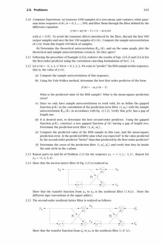
2.9. Problems 103
2.10 Computer Experiment. (a) Generate 1000 samples of a zero-mean, unit-variance, white gaus-sian noise sequence x(n), n = 0,1, . . . ,999, and filter them through the filter defined by thedifference equation:
y(n)= ay(n− 1)+(1− a)x(n)with a = 0.95. To avoid the transient effects introduced by the filter, discard the first 900output samples and save the last 100 samples of y(n). Compute the sample autocorrelationof y(n) from this length-100 block of samples.
(b) Determine the theoretical autocorrelation Ryy(k), and on the same graph, plot thetheoretical and sample autocorrelations versus k. Do they agree?
2.11 Following the procedure of Example (2.6.l), rederive the results of Eqs. (2.6.2) and (2.6.4) forthe first-order predictor using the correlation canceling formulation of Sect. 1.4.
2.12 Let y(n)= (1,1,1,1) forn = 0,1,2,3. We want to “predict” the fifth sample in this sequence,that is, the value of y(4).
(a) Compute the sample autocorrelation of this sequence.
(b) Using the Yule-Walker method, determine the best first order predictor of the form
y(n)= −a1y(n− 1)
What is the predicted value of the fifth sample? What is the mean-square predictionerror?
(c) Since we only have sample autocorrelations to work with, let us define the gappedfunction g(k) as the convolution of the prediction-error filter (1, a1) with the sampleautocorrelation Ryy(k), in accordance with Eq. (2.7.2). Verify that g(k) has a gap oflength one.
(d) It is desired next, to determine the best second-order predictor. Using the gappedfunction g(k), construct a new gapped function g′(k) having a gap of length two.Determine the prediction-error filter (1, a′1, a′2).
(e) Compute the predicted value of the fifth sample in this case, and the mean-squareprediction error. Is the predicted fifth value what you expected? Is the value predictedby the second-order predictor “better” than that predicted by the first-order predictor?
(f) Determine the zeros of the prediction filter (1, a′1, a′2) and verify that they lie insidethe unit circle in the z-plane.
2.13 Repeat parts (a) and (b) of Problem 2.12 for the sequence yn = (−1,1,−1,1). Repeat foryn = (1,2,3,4).
2.14 Show that the inverse lattice filter of Fig. 2.23 is realized as
Show that the transfer function from en to yn is the synthesis filter 1/A(z). (Note thedifferent sign conventions at the upper adder.)
2.15 The second-order synthesis lattice filter is realized as follows:
Show that the transfer function from e′n to yn is the synthesis filter 1/A′(z).

104 2. Some Signal Processing Applications
2.16 Consider the second-order prediction-error filter A′(z) given in Eq. (2.7.6). Show that thequadratic norm of the synthesis filter 1/A′(z) is given by∥∥∥∥ 1
A′
∥∥∥∥2
=∮
u.c.
1
A′(z)A′(z−1)dz
2πjz= 1
(1− γ21)(1− γ2
2)
where γ1 and γ2 are the corresponding reflection coefficients. (Hint: factor A′(z) into itszeros, which are both inside the unit circle, perform the indicated contour integration, andrewrite the result in terms of γ1 and γ2.) This result was used in Section 2.8 in the discussionof the channel errors in DPCM systems.
2.10 References
1. A. Papoulis, Probability, Random Variables, and Stochastic Processes, New York, McGraw-Hill, 1965.
2. A. V. Oppenheim and R. W. Schafer, Digital Signal Processing, Englewood Cliffs, NJ, Prentice-Hall, 1975.
3. S. Tretter, Introduction to Discrete-Time Signal Processing, New York, Wiley, 1974.
4. K. J. Åstrom and P. Eykhoff, System Identification—A Survey, Automatica, 7, 123–162(1971).
5. P. Eykhoff, System Identification: Parameter and State Estimation, New York, Wiley, 1974.
6. G. C. Goodwin and R. L. Payne, Dynamic System Identification, Experimental Design andData Analysis, New York, Academic, 1977.
7. L. Ljung and T. Soderstrom, Theory and Practice of Recursive Identification, Cambridge,MA, MIT Press, 1983.
8. L. Ljung, System Identification: Theory for the User, Englewood Cliffs, NJ, Prentice-Hall,1987.
9. T. Soderstrom and P. Stoica, System Identification, Englewood Cliffs, NJ, Prentice-Hall, 1987.
10. G. C. Goodwin and K. S. Sin, Adaptive Filtering, Prediction, and Control, Englewood Cliffs,NJ, Prentice-Hall, 1984.
11. M. I. Skolnik, Introduction to Radar Systems, New York, McGraw-Hill, 1980.
12. L. Rabiner and B. Gold, Theory and Application of Digital Signal Processing, Englewood-Cliffs, NJ, Prentice-Hall, 1975.
13. L. B. Jackson, Roundoff Noise Analysis for Fixed-Point Digital Filters Realized in Cascadeor Parallel Form, IEEE Trans. Audio Electroacoust., AU-18, 107–122 (1970).
14. B. Liu, Effect of Finite Word Length on the Accuracy of Digital Filters—A Review, IEEE Trans.Circuit Th., CT-18, 670–677 (1971).
15. C. T. Mullis and R. A. Roberts, Synthesis of Minimum Roundoff Noise Fixed Point DigitalFilters, IEEE Trans. Circuits Syst., CAS-23, 551–562 (1976).
16. S. Y. Hwang, Roundoff Noise in State-Space Digital Filtering: A General Analysis, IEEE Trans.Acoust., Speech, Signal Process., ASSP-24, 256–262 (1976).
17. A. B. Sripad and D. L. Snyder, A Necessary and Sufficient Condition for Quantization Errorsto Be Uniform and White, IEEE Trans. Acoust., Speech, Signal Process., ASSP-25, 442–448(1977).
18. T. L. Chang and S. A. White, An Error Cancellation Digital Filter Structure and its DistributedArithmetic Implementation, IEEE Trans. Circuits Syst., CAS-28, 339–342 (1981).
19. W. E. Higgins and D. C. Munson, Jr., Noise Reduction Strategies for Digital Filters: ErrorSpectrum Shaping versus the Optimal Linear State-Space Formulation, IEEE Trans. Acoust.,Speech, Signal Process., ASSP-30, 963–973 (1982).
20. C. T. Mullis and R. A. Roberts, An Interpretation of Error Spectrum Shaping in Digital Filters,IEEE Trans. Acoust., Speech, Signal Process., ASSP-30, 1013–1015 (1982).
2.10. References 105
21. R. A. Roberts and C. T. Mullis, Digital Signal Processing, Reading, MA, Addison-Wesley,1987.
22. E. Robinson and S. Treitel, Maximum Entropy and the Relationship of the Partial Autocor-relation to the Reflection Coefficients of a Layered System, IEEE Trans. Acoust., Speech,Signal Process., ASSP-28, 22 (1980).
23. T. Kailath, A Theorem of I. Schur and Its Impact on Modern Signal Processing, in I. Gohberg,Ed., I. Schur Methods in Operator Theory and Signal Processing, Operator Theory: Advancesand Applications, vol. 18, Boston, Birkhauser, 1986.
24. J. L. Flanagan, et al., Speech Coding, IEEE Trans. Commun., COM-27, 710–736, (1979).
25. N. S. Jayant and P. Noll, Digital Coding of Waveforms, Englewood Cliffs, NJ, Prentice-Hall,1984.
26. A. K. Jain, Image Data Compression: A Review, Proc. IEEE, 69, 349–389 (1981).
27. J. W. Modestino and D. G. Daut, Combined Source-Channel Coding of Images, IEEE Trans.Commun., COM-27, 1644–1659 (1979).
28. D. G. Daut and J. W. Modestino, Two-Dimensional DPCM Image Transmission over FadingChannels, IEEE Trans. Commun., COM-31, 315–328 (1983).

3Spectral Factorization
In this chapter, we discuss the concept of minimum-phase signals and filters, state thespectral factorization theorem, and demonstrate its importance in making signal mod-els, and present a proof of the minimum-phase property of the prediction-error filter oflinear prediction.
3.1 Minimum-Phase Signals and Filters
A minimum-phase sequence a = [a0, a1, . . . , aM] has a z-transform with all its zerosinside the unit circle in the complex z-plane
A(z)= a0+a1z−1+· · ·+aMz−M = a0(1−z1z−1)(1−z2z−1)· · · (1−zMz−1) (3.1.1)
with |zi| < 1, i = 1,2, . . . ,M. Such a polynomial is also called a minimum-delay polyno-mial. Define the following related polynomials:
A∗(z) = a∗0 + a∗1 z−1 + · · · + a∗Mz−M = complex-conjugated coefficients
A(z) = a∗0 + a∗1 z+ · · · + a∗MzM = conjugated and reflected
AR(z) = a∗M + a∗M−1z−1 + · · · + a∗0 z−M = reversed and conjugated
We note the relationships:
A(z)= A∗(z−1) and AR(z)= z−MA(z)= z−MA∗(z−1) (3.1.2)
We also note that when we set z = ejω to obtain the corresponding frequency re-sponses, A(ω) becomes the complex conjugate of A(ω)
A(ω)= A(ω)∗ (3.1.3)
It is easily verified that all these polynomials have the same magnitude spectrum:
|A(ω)|2 = |A(ω)|2 = |A∗(ω)|2 = |AR(ω)|2 (3.1.4)
For example, in the case of a doublet a = (a0, a1) and its reverse aR = (a∗1 , a∗0 ), weverify explicitly
|A(ω)|2 = A(ω)A(ω)∗ = (a0 + a1e−jω)(a∗0 + a∗1 ejω)= (a∗1 + a∗0 e−jω)(a1 + a0ejω)
= AR(ω)AR(ω)∗= |AR(ω)|2

3.2. Partial Energy and Minimal Delay 107
Thus, on the basis the magnitude spectrum, one cannot distinguish the doubleta = (a0, a1) from its reverse aR = (a∗1 , a∗0 ). In the more general case of a polynomialof degree M, factored into doublets as in Eq. (3.1.1), we note that each doublet can bereplaced by its reverse
(1,−zi)→ (−z∗i ,1) or (1− ziz−1)→ (−z∗i + z−1)
without affecting the overall magnitude spectrum |A(ω)|2. Since there are M suchfactors, there will be a total of 2M different Mth degree polynomials, or equivalently,2M different length-(M+1) sequences, all having the same magnitude spectrum. Everytime a factor (1 − ziz−1) is reversed to become (−z∗i + z−1), the corresponding zerochanges from z = zi to z = 1/z∗i . If zi is inside the unit circle, the 1/z∗i is outside, asshown
To enumerate all these sequences, start by taking all zeros zi to be inside the unitcircle and successively keep reversing each factor until all 2M possibilities have beenexhausted. At the last step, all the factors will have been flipped, corresponding toall the zeros being outside the unit circle. The resulting polynomial and sequence arereferred to as having maximal phase, or maximal delay. As an example consider the twodoublets
a = (2,1) and b = (3,2)and form the four different sequences, where ∗ denotes convolution:
c0 = a∗ b = (2,1)∗(3,2)= (6,7,2), C0(z)= A(z)B(z)c1 = aR ∗ b = (1,2)∗(3,2)= (3,8,4), C1(z)= AR(z)B(z)c2 = a∗ bR = (2,1)∗(2,3)= (4,8,3), C2(z)= A(z)BR(z)c3 = aR ∗ bR = (1,2)∗(2,3)= (2,7,6), C3(z)= A(z)B(z)
All four sequences have the same magnitude spectrum.
3.2 Partial Energy and Minimal Delay
Since the total energy of a sequence a = (a0, a1, . . . , aM) is given by Parseval’s equality
M∑m=0
|am|2 =∫ π−π|A(ω)|2 dω
2π
it follows that all of the above 2M sequences, having the same magnitude spectrum, willalso have the same total energy. However, the distribution of the total energy over timemay be different. And this will allow an alternative characterization of the minimumphase sequences, first given by Robinson. Define the partial energy by
Pa(n)=n∑m=0
|am|2 = |a0|2 + |a1|2 + · · · + |an|2 , n = 0,1, . . . ,M

108 3. Spectral Factorization
then, for the above example, the partial energies for the four different sequences aregiven in the table
c0 c1 c2 c3
P(0) 36 9 16 4P(1) 85 73 80 53P(2) 89 89 89 89
We note that c0 which has both its zeros inside the unit circle (i.e., minimal phase) isalso the sequence that has most of its energy concentrated at the earlier times, that is,it makes its impact as early as possible, with minimal delay. In contrast, the maximal-phase sequence c3 has most of its energy concentrated at its tail thus, making most ofits impact at the end, with maximal delay.
3.3 Invariance of the Autocorrelation Function
This section presents yet another characterization of the above class of sequences. Itwill be important in proving the minimum-phase property of the linear prediction filters.
The sample autocorrelation of a (possibly complex-valued) sequence a = (a0, a1, . . . , aM)is defined by
Raa(k) =M−k∑n=0
an+ka∗n , for 0 ≤ k ≤M
Raa(k) = Raa(−k)∗ , for −M ≤ k ≤ −1
(3.3.1)
It is easily verified that the corresponding power spectral density is factored as
Saa(z)=M∑
k=−MRaa(k)z−k = A(z)A(z) (3.3.2)
The magnitude response is obtained by setting z = ejω
Saa(ω)= |A(ω)|2 (3.3.3)
with an inversion formula
Raa(k)=∫ π−π|A(ω)|2ejωk dω
2π(3.3.4)
It follows from Eq. (3.3.4) that the above 2M different sequences having the samemagnitude spectrum, also have the same sample autocorrelation. They cannot be distin-guished on the basis of their autocorrelation. Therefore, there are 2M different spectralfactorizations of Saa(z) of the form
Saa(z)= A(z)A(z) (3.3.5)
but there is only one with minimum-phase factors. The procedure for obtaining it isstraightforward: Find the zeros of Saa(z), which come in pairs zi and 1/z∗i , thus, thereare 2M such zeros. And, group those that lie inside the unit circle into a common factor.This defines A(z) as a minimum phase polynomial.
3.4 Minimum-Delay Property
Here, we discuss the effect of flipping a zero from the inside to the outside of the unitcircle, on the minimum-delay and minimum-phase properties of the signal. Suppose

3.5. Minimum-Phase Property 109
A(z) is of degreeM and has a zero z1 inside the unit circle. Let B(z) be the polynomialthat results by flipping this zero to the outside; that is, z1 → 1/z∗1
A(z) = (1− z1z−1)F(z)
B(z) = (−z∗1 + z−1)F(z)(3.4.1)
where F(z) is a polynomial of degree M − 1. Both A(z) and B(z) have the same mag-nitude spectrum. We may think of this operation as sending A(z) through an allpassfilter
B(z)= −z∗1 + z−1
1− z1z−1A(z)
In terms of the polynomial coefficients, Eq. (3.4.1) becomes
an = fn − z1fn−1
bn = −z∗1 fn + fn−1
(3.4.2)
for n = 0,1, . . . ,M, from which we obtain
|an|2 − |bn|2 =(1− |z1|2
)(|fn|2 − |fn−1|2)
(3.4.3)
Summing to get the partial energies, Pa(n)=∑nm=0 |am|2, we find
Pa(n)−Pb(n)=(1− |z1|2
)|fn|2 , n = 0,1, . . . ,M (3.4.4)
Thus, the partial energy of the sequence a remains greater than that of b for all timesn; that is, A(z) is of earlier delay than B(z). The total energy is, of course, the sameas follows from the fact that F(z) is of degree M − 1, thus, missing the Mth term orfM = 0. We have then
Pa(n)≥ Pb(n) , n = 0,1, . . . ,M
and in particularPa(M)= Pb(M) and Pa(0)≥ Pb(0)
The last inequality can also be stated as |a0| ≥ |b0|, and will be important in ourproof of the minimum-phase property of the prediction-error filter of linear prediction.
3.5 Minimum-Phase Property
The effect of reversing the zero z1 on the phase responses ofA(z) andB(z) of Eq. (3.4.1)can be seen as follows. For z = ejω, define the phase lag as the negative of the phaseresponse
A(ω) = |A(ω)|ejArg(ω)
θA(ω) = −Arg(ω)= phase-lag response
and similarly for B(z). SinceA(ω) and B(ω) have the same magnitude, they will differonly by a phase
A(ω)B(ω)
= ej(θB−θA) = 1− z1e−jω
−z∗1 + e−jω= ejω − z1
1− z∗1 ejω= ejφ(ω)
whereφ(ω) is the phase-response of the all-pass factor (ejω−z1)/(1−z∗1 ejω), so thatθB(ω)−θA(ω)= φ(ω). By taking derivatives with respect toω in the above definitionof φ(ω), it can be easily shown that
dφ(ω)dω
= 1− |z1|2∣∣ejω − z1∣∣2 > 0

110 3. Spectral Factorization
which shows thatφ(ω) is an increasing function ofω. Thus, over the frequency interval0 ≤ ω ≤ π, we have φ(ω)≥ φ(0). It can be verified easily that φ(0)= −2φ0, whereφ0 is the angle with the x-axis of the line between the points z1 and 1, as shown in thefigure below.
Thus, we have θB − θA ≥ φ ≥ −2φ0. The angle φ0 is positive, if z1 lies within theupper half semi-circle, and negative, if it lies in the lower semi-circle; and, φ0 is zeroif z1 lies on the real axis. If z1 is real-valued, then θB ≥ θA for 0 ≤ ω ≤ π. If z1
is complex valued and we consider the combined effect of flipping the zero z1 and itsconjugate z∗1 , that is, A(z) and B(z) are given by
A(z) = (1− z1z−1)(1− z∗1 z−1)F(z)
B(z) = (−z∗1 + z−1)(−z1 + z−1)F(z)
then, for the phase of the combined factor
ejφ(ω) = ejω − z1
1− z∗1 ejω· e
jω − z∗11− z1ejω
we will have φ(ω)≥ (−2φ0)+(2φ0)= 0, so that θB(ω)−θA(ω)= φ(ω)≥ 0.Thus, the phase lag of A(z) remains smaller than that of B(z). The phase-lag curve
for the case when A(z) has all its zeros inside the unit circle will remain below all theother phase-lag curves. The term minimum-phase strictly speaking means minimumphase lag (over 0 ≤ω ≤ π).
3.6 Spectral Factorization Theorem
We finish our digression on minimum-phase sequences by quoting the spectral factor-ization theorem [5].
Any rational power spectral density Syy(z) of a (real-valued) stationary signal yncan be factored in a minimum-phase form
Syy(z)= σ2εB(z)B(z−1) (3.6.1)
where
B(z)= N(z)D(z)
(3.6.2)
with both D(z) and N(z) being minimum-phase polynomials; that is, having all theirzeros inside the unit circle. By adjusting the overall constant σ2
ε , both D(z) and N(z)may be taken to be monic polynomials. Then, they are unique.
This theorem guarantees the existence of a causal and stable random signal generatorfilter B(z) for the signal yn of the type discussed in Section 1.11:

3.6. Spectral Factorization Theorem 111
with εn white noise of variance σ2ε . The minimum-phase property of B(z) also guaran-
tees the stability and causality of the inverse filter 1/B(z), that is, the whitening filter
The proof of the spectral factorization theorem is straightforward. Since Syy(z) isthe power spectral density of a (real-valued) stationary process yn, it will satisfy thesymmetry conditions Syy(z)= Syy(z−1). Therefore, if zi is a zero then 1/zi is alsoa zero, and if zi is complex then the reality of Ryy(k) implies that z∗i will also be azero. Thus, both zi and 1/z∗i are zeros. Therefore, the numerator polynomial of Syy(z)is of the type of Eq. (3.3.5) and can be factored into its minimum phase polynomialsN(z)N(z−1). This is also true of the denominator of Syy(z).
All sequential correlations in the original signal yn arise from the filtering action ofB(z) on the white-noise input εn. This follows from Eq. (2.1.14):
Ryy(k)= σ2ε
∑nbn+kbn , B(z)=
∞∑n=0
bnz−n (3.6.3)
Effectively, we have modeled the statistical autocorrelationRyy(k) by the sample au-tocorrelation of the impulse response of the synthesis filter B(z). Since B(z) is causal,such factorization corresponds to an LU, or Cholesky, factorization of the autocorrela-tion matrix.
This matrix representation can be seen as follows: Let B be the lower triangularToeplitz matrix defined exactly as in Eq. (1.11.2)
bni = bn−iand let the autocorrelation matrix of yn be
Ryy(i, j)= Ryy(i− j)
Then, the transposed matrix BT will have matrix elements
(BT)ni= bi−nand Eq. (3.6.3) can be written in the form
Ryy(i, j) = Ryy(i− j)= σ2ε
∑nbn+i−jbn = σ2
ε
∑kbi−kbj−k
= σ2ε
∑k(B)ik(BT)kj= σ2
ε(BBT)ij
Thus, in matrix notationRyy = σ2
εBBT (3.6.4)
This equation is a special case of the more general LU factorization of the Gram-Schmidt construction given by Eq. (1.5.17). Indeed, the assumption of stationarity im-plies that the quantity
σ2ε = E[ε2
n]
is independent of the time n, and therefore, the diagonal matrix Rεε of Eq. (1.5.17)becomes a multiple of the identity matrix.

112 3. Spectral Factorization
3.7 Minimum-Phase Property of the Prediction-Error Filter
As mentioned in Section 2.8, the minimum-phase property of the prediction-error filterA(z) of linear prediction is an important property because it guarantees the stabilityof the causal inverse synthesis filter 1/A(z). There are many proofs of this propertyin the literature [6–10]. Here, we would like to present a simple proof [11] which isbased directly on the fact that the optimal prediction coefficients minimize the mean-square prediction error. Although we have only discussed first and second order linearpredictors, for the purposes of this proof we will work with the more general case of anMth order predictor defined by
yn = −[a1yn−1 + a2yn−2 + · · · + aMyn−M]which is taken to represent the best prediction of yn based on the past M samplesYn = {yn−1, yn−2, . . . , yn−M}. The corresponding prediction error is
en = yn − yn = yn + a1yn−1 + a2yn−2 + · · · + aMyn−MThe best set of prediction coefficients {a1, a2, . . . aM} is found by minimizing the
mean-square prediction error
E(a1, a2, . . . aM) = E[e∗nen]=M∑
m,k=0
a∗mE[y∗n−myn−k]ak
=M∑
m,k=0
a∗mRyy(k−m)ak =M∑
m,k=0
a∗mRyy(m− k)ak(3.7.1)
where we set a0 = 1. For the proof of the minimum phase property, we do not needthe explicit solution of this minimization problem; we only use the fact that the optimalcoefficients minimize Eq. (3.7.1). The key to the proof is based on the observation that(3.7.1) can be written in the alternative form
E(a)=M∑
k=−MRyy(k)Raa(k) (3.7.2)
where Raa(k) is the sample autocorrelation of the prediction-error filter sequence a =[1, a1, a2, . . . , aM]T as defined in Eq. (3.3.1). The equivalence of Eqs. (3.7.1) and (3.7.2)can be seen easily, either by rearranging the summation indices of (3.7.1), or by usingthe results of Problems 2.3 and 2.5.
Example 3.7.1: We demonstrate this explicitly for the M = 2 case. Using the definition (3.3.1)we have
Raa(0) = |a0|2 + |a1|2 + |a2|2 = 1+ |a1|2 + |a2|2
Raa(1) = Raa(−1)∗= a1a∗0 + a2a∗1 = a1 + a2a∗1
Raa(2) = Raa(−2)∗= a2a∗0 = a2
Since yn is real-valued stationary, we have Ryy(k)= Ryy(−k). Then, Eq. (3.7.1) becomesexplicitly
E(a)=M∑
m,k=0
a∗mRyy(m− k)ak = [1, a∗1 , a∗2 ]⎡⎢⎣ Ryy(0) Ryy(1) Ryy(2)Ryy(1) Ryy(0) Ryy(1)Ryy(0) Ryy(1) Ryy(2)
⎤⎥⎦⎡⎢⎣ 1a1
a2
⎤⎥⎦= Ryy(0)[1+ a∗1 a1 + a∗2 a2]+Ryy(1)
[(a1 + a2a∗1 )+(a∗1 + a∗2 a1)
]+Ryy(2)[a2 + a∗2 ]= Ryy(0)Raa(0)+Ryy(1)
[Raa(1)+Raa(−1)
]+Ryy(2)[Raa(2)+Raa(−2)] ��

3.8. Problems 113
Let a = [1, a1, a2, . . . , aM]T be the optimal set of coefficients that minimizes E(a)and let zi, i = 1,2 . . . ,M, be the zeros of the corresponding prediction-error filter:
1+ a1z−1 + a2z−2 + · · · + aMz−M = (1− z1z−1)(1− z2z−1)· · · (1− zMz−1) (3.7.3)
Reversing any one of the zero factors in this equation, that is, replacing (1−ziz−1) byits reverse (−z∗i +z−1), results in a sequence that has the same sample autocorrelationas a. As we have seen, there are 2M such sequences, all with the same sample autocorre-lation. We would like to show that among these, a is the one having the minimum-phaseproperty.
To this end, let b = [b0, b1, . . . bM]T be any one of these 2M sequences, and definethe normalized sequence
c = b/b0 = [1, b1/b0, b2/b0, . . . bM/b0]T (3.7.4)
Using the fact that b has the same sample autocorrelation as a, we find for the sampleautocorrelation of c :
Rcc(k)= Rbb(k)/|b0|2 = Raa(k)/|b0|2 (3.7.5)
The performance index (3.7.2) evaluated at c is then
E(c)=M∑
k=−MRyy(k)Rcc(k)=
M∑k=−M
Ryy(k)Raa(k)/|b0|2 (3.7.6)
or,E(c)= E(a)/|b0|2 (3.7.7)
Since a minimizes E, it follows that E(c)≥ E(a). Therefore, Eq. (3.7.7) implies that
|b0| ≤ 1 (3.7.8)
This must be true of all bs in the above class. Eq. (3.7.8) then, immediately implies theminimum-phase property of a. Indeed, choosing b to be that sequence obtained from(3.7.3) by reversing only the ith zero factor (1− ziz−1) and not the other zero factors,it follows that
b0 = −z∗iand therefore Eq. (3.7.8) implies that
|zi| ≤ 1 (3.7.9)
which shows that all the zeros of A(z) are inside the unit circle and thus, A(z) hasminimum phase. An alternative proof based on the Levinson recursion and Rouche’stheorem of complex analysis will be presented in Chapter 5.
3.8 Problems
3.1 Prove Eq. (3.3.2).
3.2 Using Eq. (3.4.1), show Eqs. (3.4.3) and (3.4.4).
3.3 A random signal yn has autocorrelation function
Ryy(k)= (0.5)|k| , for all k
Find a random signal generator model for yn.

114 3. Spectral Factorization
3.4 Repeat Problem 3.3 when
Ryy(k)= (0.5)|k|+(−0.5)|k| , for all k
3.5 The autocorrelation function of a stationary random signal y(n) is
Ryy(k)= 1−R2
1+R2R|k| cos(πk/2) , for all k , where 0 < R < 1
(a) Compute the power spectrum Syy(ω) of y(n) and sketch it versus frequency forvarious values of R.
(b) Find the signal generator filter for y(n) and determine its difference equation and itspoles and zeros.
3.6 A stationary random signal yn has a rational power spectral density given by
Syy(z)= 2.18− 0.6(z+ z−1)1.25− 0.5(z+ z−1)
Determine the signal model filter B(z) and the parameter σ2ε . Write the difference equation
generating yn.
3.7 Let yn = cxn + vn. It is given that
Sxx(z)= Q(1− az−1)(1− az) , Svv(z)= R , Sxv(z)= 0
where a, c,Q,R are known constants (assume |a| < 1) for the stability of xn.)
(a) Show that the filter model for yn is of the form
B(z)= 1− fz−1
1− az−1
where f has magnitude less than one and is the solution of the algebraic quadraticequation
aR(1+ f2)= [c2Q +R(1+ a2)
]f
and show that the other solution has magnitude greater than one.
(b) Show that f can alternatively be expressed as
f = RaR+ c2P
where P is the positive solution of the quadratic equation
Q = P− PRa2
R+ c2P
known as the algebraic Riccati equation. Show that the other solution is negative.Show that the positivity of P is essential to guarantee that f has magnitude less thanone.
(c) Show that the scale factor σ2ε that appears in the spectral factorization (3.6.1) can also
be expressed in terms of P as
σ2ε = R+ c2P
The above method of solution of the spectral factorization problem by reducing it to thesolution of an algebraic Riccati equation is quite general and can be extended to the multi-channel case.

3.9. References 115
3.8 Consider a stable (but not necessarily causal) sequence bn, −∞ < n <∞ with a z-transformB(z)
B(z)=∞∑
n=−∞bnz−n
Define an infinite Toeplitz matrix B by
Bni = bn−i , for −∞ < n, i <∞
This establishes a correspondence between stable z-transforms or stable sequences andinfinite Toeplitz matrices.
(a) Show that if the sequence bn is causal, then B is lower triangular, as shown here
In the literature of integral operators and kernels, such matrices are rotated by 90o
degrees as shown:
so that the n axis is the horizontal axis. For this reason, in that context they are called“right Volterra kernel,” or “causal kernels.”
(b) Show that the transposed BT corresponds to the reflected (about the origin) sequenceb−n and to the z-transform B(z−1).
(c) Show that the convolution of two sequences an and bn
cn = an ∗ bn or C(z)= A(z)B(z)
corresponds to the commutative matrix product
C = AB = BA
3.9 Prove Eq. (3.7.2) for anyM.
3.9 References
1. E. Robinson and S. Treitel, Geophysical Signal Analysis, Englewood Cliffs, NJ, Prentice-Hall,1980.
2. E. A. Robinson, Statistical Communication and Detection, New York, Hafner, 1967.
3. E. A. Robinson, Multichannel Time-Series Analysis with Digital Computer Programs, (2nded.), Houston, TX, Goose Pond Press, 1983.
4. A. V. Oppenheim and R. W. Schafer, Digital Signal Processing, Englewood Cliffs, NJ, Prentice-Hall, 1975.
5. P. Whittle, Prediction and Regulation, New York, Van Nostrand Reinhold, 1963.
6. J. D. Markel and A. H. Gray, Jr., Linear Prediction of Speech, New York, Springer-Verlag,1976.
7. E. A. Robinson and S. Treitel, Digital Signal Processing in Geophysics, in A. V. Oppenheim,Ed., Applications of Digital Signal Processing, Englewood Cliffs, NJ, Prentice-Hall, 1978.
8. S. Lang and J. McClellan, A Simple Proof of Stability for All-Pole Linear Prediction Models,Proc. IEEE, 67, 860-861 (1979).

116 3. Spectral Factorization
9. S. Kay and L. Pakula, Simple Proofs of the Minimum Phase Property of the Prediction ErrorFilter, IEEE Trans. Acoust., Speech, Signal Process., ASSP-31, 501 (1983).
10. P. Stoica and A. Nehorai, On Stability and Root Location of Linear Prediction Models, IEEETrans. Acoust., Speech, Signal Process., ASSP-35, 582 (1987).
11. S. J. Orfanidis, A Proof of the Minimal Phase Property of the Prediction Error Filter, Proc.IEEE, 71, 905 (1983).

4Linear Estimation of Signals
The problem of estimating one signal from another is one of the most important insignal processing. In many applications, the desired signal is not available or observabledirectly. Instead, the observable signal is a degraded or distorted version of the originalsignal. The signal estimation problem is to recover, in the best way possible, the desiredsignal from its degraded replica.
We mention some typical examples: (1) The desired signal may be corrupted bystrong additive noise, such as weak evoked brain potentials measured against the strongbackground of ongoing EEGs; or weak radar returns from a target in the presence ofstrong clutter. (2) An antenna array designed to be sensitive towards a particular “look”direction may be vulnerable to strong jammers from other directions due to sidelobeleakage; the signal processing task here is to null the jammers while at the same timemaintaining the sensitivity of the array towards the desired look direction. (3) A signaltransmitted over a communications channel can suffer phase and amplitude distortionsand can be subject to additive channel noise; the problem is to recover the transmittedsignal from the distorted received signal. (4) A Doppler radar processor tracking amoving target must take into account dynamical noise—such as small purely randomaccelerations—affecting the dynamics of the target, as well as measurement errors. (5)An image recorded by an imaging system is subject to distortions such as blurring due tomotion or to the finite aperture of the system, or other geometric distortions; the prob-lem here is to undo the distortions introduced by the imaging system and restore theoriginal image. A related problem, of interest in medical image processing, is that of re-constructing an image from its projections. (6) In remote sensing and inverse scatteringapplications, the basic problem is, again, to infer one signal from another; for example,to infer the temperature profile of the atmosphere from measurements of the spectraldistribution of infrared energy; or to deduce the structure of a dielectric medium, suchas the ionosphere, by studying its response to electromagnetic wave scattering; or, inoil exploration to infer the layered structure of the earth by measuring its response toan impulsive input near its surface.
In this chapter, we pose the signal estimation problem and discuss some of thecriteria used in the design of signal estimation algorithms.
We do not present a complete discussion of all methods of signal recovery and es-timation that have been invented for applications as diverse as those mentioned above.Our emphasis is on traditional linear least-squares estimation methods, not only be-cause they are widely used, but also because they have served as the motivating forcefor the development of other estimation techniques and as the yardstick for evaluatingthem.
We develop the theoretical solution of the Wiener filter both in the stationary andnonstationary cases, and discuss its connection to the orthogonal projection, Gram-Schmidt constructions, and correlation canceling ideas of Chapter 1. By means of an

118 4. Linear Estimation of Signals
example, we introduce Kalman filtering concepts and discuss their connection to Wienerfiltering and to signal modeling. Practical implementations of the Wiener filter are dis-cussed in Chapters 5 and 7. Other signal recovery methods for deconvolution appli-cations that are based on alternative design criteria are briefly discussed in Chapter5, where we also discuss some interesting connections between Wiener filtering/linearprediction methods and inverse scattering methods.
4.1 Linear and Nonlinear Estimation of Signals
The signal estimation problem can be stated as follows: We wish to estimate a randomsignal xn on the basis of available observations of a related signal yn. The availablesignal yn is to be processed by an optimal processor that produces the best possibleestimate of xn:
The resulting estimate xn will be a function of the observations yn. If the optimalprocessor is linear, such as a linear filter, then the estimate xn will be a linear functionof the observations. We are going to concentrate mainly on linear processors. However,we would like to point out that, depending on the estimation criterion, there are caseswhere the estimate xn may turn out to be a nonlinear function of the yns.
We discuss briefly four major estimation criteria for designing such optimal proces-sors. They are:
(1) The maximum a posteriori (MAP) criterion.(2) The maximum likelihood (ML) criterion.(3) The mean square (MS) criterion.(4) The linear mean-square (LMS) criterion.
The LMS criterion is a special case of the MS criterion. It requires, a priori, that theestimate xn be a linear function of the yns.† The main advantage of the LMS processoris that it requires only knowledge of second order statistics for its design, whereas theother, nonlinear, processors require more detailed knowledge of probability densities.
To explain the various estimation criteria, let us assume that the desired signal xnis to be estimated over a finite time interval na ≤ n ≤ nb Without loss of generality, wemay assume that the observed signal yn is also available over the same interval. Definethe vectors
x =
⎡⎢⎢⎢⎢⎢⎣xnaxna+1
...xnb
⎤⎥⎥⎥⎥⎥⎦ , y =
⎡⎢⎢⎢⎢⎢⎣ynayna+1
...ynb
⎤⎥⎥⎥⎥⎥⎦For each value of n, we seek the functional dependence
xn = xn(y)
of xn on the given observation vector y that provides the best estimate of xn.
1. The criterion for the MAP estimate is to maximize the a posteriori conditionaldensity of xn given that y already occurred; namely,
p(xn|y)= maximum (4.1.1)
†Note that the acronym LMS is also used in the context of adaptive filtering, for least mean-square.

4.1. Linear and Nonlinear Estimation of Signals 119
in other words, the optimal estimate xn is that xn that maximizes this quantityfor the given vector y; xn is therefore the most probable choice resulting from thegiven observations y.
2. The ML criterion, on the other hand, selects xn to maximize the conditional densityof y given xn, that is,
p(y|xn)= maximum (4.1.2)
This criterion selects xn as though the already collected observations y were themost likely to occur.
3. The MS criterion minimizes the mean-square estimation error
E = E[e2n]= min, where en = xn − xn (4.1.3)
that is, the best choice of the functional dependence xn = xn(y) is sought thatminimizes this expression. We know from our results of Section 1.4 that therequired solution is the corresponding conditional mean
xn = E[xn|y]= MS estimate (4.1.4)
computed with respect to the conditional density p(xn|y).4. Finally, the LMS criterion requires the estimate to be a linear function of the ob-
servations
xn =nb∑i=na
h(n, i)yi (4.1.5)
For each n, the weights h(n, i), na ≤ i ≤ nb are selected to minimize the mean-square estimation error
E = E[e2n]= E
[(xn − xn)2] = minimum (4.1.6)
With the exception of the LMS estimate, all other estimates xn(y) are, in general,nonlinear functions of y.
Example 4.1.1: If both xn and y are zero-mean and jointly gaussian, then Examples 1.4.1 and1.4.2 imply that the MS and LMS estimates of xn are the same. Furthermore, since p(xn|y)is gaussian it will be symmetric about its maximum, which occurs at its mean, that is, atE[xn|y]. Therefore, the MAP estimate of xn is equal to the MS estimate. In conclusion, forzero-mean jointly gaussian xn and y, the three estimates MAP, MS, and LMS coincide. ��
Example 4.1.2: To see the nonlinear character and the differences among the various estimates,consider the following example: A discrete-amplitude, constant-in-time signal x can takeon the three values
x = −1, x = 0, x = 1
each with probability of 1/3. This signal is placed on a known carrier waveform cn andtransmitted over a noisy channel. The received samples are of the form
yn = cnx+ vn , n = 1,2, . . . ,M
where vn are zero-mean white gaussian noise samples of variance σ2v , assumed to be inde-
pendent of x. The above set of measurements can be written in an obvious vector notation
y = cx+ v
(a) Determine the conditional densities p(y|x) and p(x|y).

120 4. Linear Estimation of Signals
(b) Determine and compare the four alternative estimates MAP, ML, MS, and LMS.
Solution: To compute p(y|x), note that if x is given, then the only randomness left in y arisesfrom the noise term v. Since vn are uncorrelated and gaussian, they will be independent;therefore,
p(y|x) = p(v)=M∏n=1
p(vn)=(2πσ2
v)−M/2
exp
⎡⎣− 1
2σ2v
M∑n=1
v2n
⎤⎦= (
2πσ2v)−M/2
exp[− 1
2σ2v
v2]= (
2πσ2v)−M/2
exp[− 1
2σ2v(y− cx)2
]
Using Bayes’ rule we find p(x|y)= p(y|x)p(x)/p(y). Since
p(x)= 1
3
[δ(x− 1)+δ(x)+δ(x+ 1)
]we find
p(x|y)= 1
A[p(y|1)δ(x− 1)+p(y|0)δ(x)+p(y| − 1)δ(x+ 1)
]where the constant A is
A = 3p(y)= 3
∫p(y|x)p(x)dx = p(y|1)+p(y|0)+p(y| − 1)
To find the MAP estimate of x, the quantity p(x|y) must be maximized with respect to x.Since the expression for p(x|y) forces x to be one of the three values +1,0,−1, it followsthat the maximum among the three coefficients p(y|1), p(y|0), p(y| − 1) will determinethe value of x. Thus, for a given y we select that x that
p(y|x)= maximum of{p(y|1), p(y|0), p(y| − 1)}
Using the gaussian nature of p(y|x), we find equivalently
(y− cx)2= minumum of{(y− c)2, y2, (y+ c)2}
Subtracting y2 from both sides, dividing by cTc, and denoting
y = cTy
cTc
we find the equivalent equation
x2 − 2xy = min{1− 2y, 0, 1+ 2y}
and in particular, applying these for +1,0,−1, we find
xMAP =
⎧⎪⎪⎪⎪⎪⎨⎪⎪⎪⎪⎪⎩1, if y >
1
2
0, if − 1
2< y <
1
2
−1, if y < −1
2
To determine the ML estimate, we must maximize p(y|x) with respect to x. The ML esti-mate does not require knowledge of the a priori probability density p(x) of x. Therefore,differentiating p(y|x) with respect to x and setting the derivative to zero gives
∂∂xp(y|x)= 0 or
∂∂x
lnp(y|x)= 0 or∂∂x(y− cx)2= 0

4.2. Orthogonality and Normal Equations 121
which gives
xML = cTy
cTc= y
The MS estimate is obtained by computing the conditional mean
E[x|y] =∫xp(x|y)dx =
∫x
1
A[p(y|1)δ(x− 1)+p(y|0)δ(x)+p(y| − 1)δ(x+ 1)
]dx
= 1
A[p(y|1)−p(y| − 1)
], or,
xMS = p(y|1)−p(y| − 1)p(y|1)+p(y|0)+p(y| − 1)
Canceling some common factors from the numerator and denominator, we find the simplerexpression
xMS = 2 sinh(2ay)ea + 2 cosh(2ay)
, where a = cTc
2σ2v
Finally, the LMS estimate can be computed as in Example 1.4.3. We find
xLMS = cTy
σ2v
σ2x+ cTc
= cTc
σ2v
σ2x+ cTc
y
All four estimates have been expressed in terms of y. Note that the ML estimate is linearbut has a different slope than the LMS estimate. The nonlinearity of the various estimatesis best seen in the following figure:
4.2 Orthogonality and Normal Equations
From now on, we will concentrate on the optimal linear estimate defined by Eqs. (4.1.5)and (4.1.6). For each time instantn at which an estimate xn is sought, the optimal weightsh(n, i), na ≤ i ≤ nb must be determined that minimize the error criterion (4.1.6). Ingeneral, a new set of optimal weights must be computed for each time instant n. In thespecial case when the processes xn and yn are stationary and the observations are avail-able for a long time, that is, na = −∞, the weights become time-invariant in the sensethat h(n, i)= h(n − i), and the linear processor becomes an ordinary time-invariantlinear filter. We will discuss the solution for h(n, i) both for the time-invariant and themore general cases. The problem of determining the optimal weights h(n, i) accordingto the mean-square error minimization criterion (4.1.6) is in general referred to as theWiener filtering problem [1–11]. An interesting historical account of the development ofthis problem and its ramifications is given in the review article by Kailath [12].
Wiener filtering problems are conventionally divided into three types:

122 4. Linear Estimation of Signals
1. The optimal smoothing problem,2. The optimal filtering problem, and3. The optimal prediction problem.
In all cases, the optimal estimate of xn at a given time instant n is given by anexpression of the form (4.1.5), as a linear combination of the available observations ynin the interval na ≤ n ≤ nb. The division into three types of problems depends onwhich of the available observations in that interval are taken into account in making upthe linear combination (4.1.5).
In the smoothing problem, all the observations in the interval [na, nb] are takeninto account. The shaded part in the following figure denotes the range of observationsthat are used in the summation of Eq. (4.1.5):
xn =nb∑i=na
h(n, i)yi
Since some of the observations are to the future of xn, the linear operation is notcausal. This does not present a problem if the sequence yn is already available andstored in memory.
The optimal filtering problem, on the other hand, requires the linear operation (4.1.5)to be causal, that is, only those observations that are in the present and past of thecurrent sample xn must be used in making up the estimate xn. This requires that thematrix of optimal weights h(n, i) be lower triangular, that is,
h(n, i)= 0, for n < i
Thus, in reference to the figure below, only the shaded portion of the observationinterval is used at the current time instant:
xn =n∑i=na
h(n, i)yi
The estimate xn depends on the present and all the past observations, from the fixedstarting point na to the current time instant n. As n increases, more and more observa-tions are taken into account in making up the estimate, and the actual computation ofxn becomes less and less efficient. It is desirable, then, to be able to recast the expres-sion for xn a time-recursive form. This is what is done in Kalman filtering. But, there isanother way to make the Wiener filter computationally manageable. Instead of allowinga growing number of observations, only the current and the past M observations yi,i = n,n− 1, . . . , n−M are taken into account. In this case, only (M + 1) filter weightsare to be computed at each time instant n. This is depicted below:
xn =n∑
i=n−Mh(n, i)yi =
M∑m=0
h(n,n−m)yn−m
This is referred to as the finite impulse response (FIR) Wiener filter. Because of itssimple implementation, the FIR Wiener filter has enjoyed widespread popularity. De-pending on the particular application, the practical implementation of the filter mayvary. In Section 4.3 we present the theoretical formulation that applies to the station-ary case; in Chapter 5 we reconsider it as a waveshaping and spiking filter and discuss anumber of deconvolution applications. In Chapter 7 we consider its adaptive implemen-tation using the Widrow-Hoff LMS algorithm and discuss a number of applications such

4.2. Orthogonality and Normal Equations 123
as channel equalization and echo cancellation; we also discuss two alternative adaptiveimplementations—the so-called “gradient lattice,” and the “recursive least-squares.”
Finally, the linear prediction problem is a special case of the optimal filtering problemwith the additional stipulation that observations only up to time instant n−D must beused in obtaining the current estimate xn; this is equivalent to the problem of predictingD units of time into the future. The range of observations used in this case is shownbelow:
xn =n−D∑i=na
h(n, i)yi
Of special interest to us will be the case of one-step prediction, corresponding to thechoice D = 1. This is depicted below:
xn =n−1∑i=na
h(n, i)yi
If we demand that the prediction be based only on the past M samples (from thecurrent sample), we obtain the FIR version of the prediction problem, referred to aslinear prediction based on the pastM samples, which is depicted below:
xn =n−1∑i=n−M
h(n, i)yi =M∑m=1
h(n,n−m)yn−m
Next, we set up the orthogonality and normal equations for the optimal weights. Webegin with the smoothing problem. The estimation error is in this case
en = xn − xn = xn −nb∑i=na
h(n, i)yi (4.2.1)
Differentiating the mean-square estimation error (4.1.6) with respect to each weighth(n, i), na ≤ i ≤ nb, and setting the derivative to zero, we obtain the orthogonalityequations that are enough to determine the weights:
∂E∂h(n, i)
= 2E[en
∂en∂h(n, i)
]= −2E[enyi]= 0 , for na ≤ i ≤ nb , or,
Rey(n, i)= E[enyi]= 0 (orthogonality equations) (4.2.2)
for na ≤ i ≤ nb. Thus, the estimation error en is orthogonal (uncorrelated) to eachobservation yi used in making up the estimate xn. The orthogonality equations provideexactly as many equations as there are unknown weights.
Inserting Eq. (4.2.1) for en, the orthogonality equations may be written in an equiv-alent form, known as the normal equations
E[(xn −
nb∑k=na
h(n, k)yk)yi
] = 0 , or,
E[xnyi]=nb∑k=na
h(n, k)E[ykyi] (normal equations) (4.2.3)
These determine the optimal weights at the current time instant n. In the vectornotation of Section 4.1, we write Eq. (4.2.3) as
E[xyT]= HE[yyT]
where H is the matrix of weights h(n, i). The optimal H and the estimate are then

124 4. Linear Estimation of Signals
x = Hy = E[xyT]E[yyT]−1y
This is identical to the correlation canceler of Section 1.4. The orthogonality equa-tions (4.2.2) are precisely the correlation cancellation conditions. Extracting the nth rowof this matrix equation, we find an explicit expression for the nth estimate xn
xn = E[xnyT]E[yyT]−1y
which is recognized as the projection of the random variable xn onto the subspacespanned by the available observations; namely, Y = {yna, yna+1, . . . , ynb}. This is ageneral result: The minimum mean-square linear estimate xn is the projection of xn ontothe subspace spanned by all the observations that are used to make up that estimate.This result is a direct consequence of the quadratic minimization criterion (4.1.6) andthe orthogonal projection theorem discussed in Section 1.5.
Using the methods of Section 1.4, the minimized estimation error at time instant nis easily computed by
En = E[enen]= E[enxn]= E[(xn −
nb∑i=na
h(n, i)yi)xn
]
= E[x2n]−
nb∑i=na
h(n, i)E[yixn]= E[x2n]−E[xnyT]E[yyT]−1E[yxn]
which corresponds to the diagonal entries of the covariance matrix of the estimationerror e :
Ree = E[eeT]= E[xxT]−E[xyT]E[yyT]−1E[yxT]
The optimum filtering problem is somewhat more complicated because of the causal-ity condition. In this case, the estimate at time n is given by
xn =n∑i=na
h(n, i)yi (4.2.4)
Inserting this into the minimization criterion (4.1.6) and differentiating with respectto h(n, i) for na ≤ i ≤ n, we find again the orthogonality conditions
Rey(n, i)= E[enyi]= 0 for na ≤ i ≤ n (4.2.5)
where the most important difference from Eq. (4.2.2) is the restriction on the range ofi, that is, en is decorrelated only from the present and past values of yi. Again, theestimation error en is orthogonal to each observation yi that is being used to make upthe estimate. The orthogonality equations can be converted into the normal equationsas follows:
E[enyi]= E[(xn −
n∑k=na
h(n, k)yk)yi
] = 0 , or,
E[xnyi]=n∑
k=nah(n, k)E[ykyi] for na ≤ i ≤ n , or, (4.2.6)
Rxy(n, i)=n∑
k=nah(n, k)Ryy(k, i) for na ≤ i ≤ n (4.2.7)

4.3. Stationary Wiener Filter 125
Such equations are generally known as Wiener-Hopf equations. Introducing the vec-tor of observations up to the current time n, namely,
yn = [yna , yna+1, . . . , yn]T
we may write Eq. (4.2.6) in vector form as
E[xnyTn]=[h(n,na), h(n,na + 1), . . . , h(n,n)
]E[ynyTn]
which can be solved for the vector of weights[h(n,na), h(n,na + 1), . . . , h(n,n)
] = E[xnyTn]E[ynyTn]−1
and for the estimate xn:xn = E[xnyTn]E[ynyTn]−1yn (4.2.8)
Again, xn is recognized as the projection of xn onto the space spanned by the ob-servations that are used in making up the estimate; namely, Yn = {yna, yna+1, . . . , yn}.This solution of Eqs. (4.2.5) and (4.2.7) will be discussed in more detail in Section 4.8,using covariance factorization methods.
4.3 Stationary Wiener Filter
In this section, we make two assumptions that simplify the structure of Eqs. (4.2.6) and(4.2.7). The first is to assume stationarity for all signals so that the cross-correlationand autocorrelation appearing in Eq. (4.2.7) become functions of the differences of theirarguments. The second assumption is to take the initial time na to be the infinite past,na = −∞, that is, the observation interval is Yn = {yi, −∞ < i ≤ n}.
The assumption of stationarity can be used as follows: Suppose we have the solutionof h(n, i) of Eq. (4.2.7) for the best weights to estimate xn, and wish to determine thebest weights h(n + d, i), na ≤ i ≤ n + d for estimating the sample xn+d at the futuretime n + d. Then, the new weights will satisfy the same equations as (4.2.7) with thechanges
Rxy(n+ d, i)=n+d∑k=na
h(n+ d, k)Ryy(k, i), for na ≤ i ≤ n+ d (4.3.1)
Making a change of variables i→ i+ d and k→ k+ d, we rewrite Eq. (4.3.1) as
Rxy(n+d, i+d)=n∑
k=na−dh(n+d, k+d)Ryy(k+d, i+d), for na−d ≤ i ≤ n (4.3.2)
Now, if we assume stationarity, Eqs. (4.2.7) and (4.3.2) become
Rxy(n− i) =n∑
k=nah(n, k)Ryy(k− i) , for na ≤ i ≤ n
Rxy(n− i) =n∑
k=na−dh(n+ d, k+ d)Ryy(k− i) , for na − d ≤ i ≤ n
(4.3.3)
If it were not for the differences in the ranges of i and k, these two equations wouldbe the same. But this is exactly what happens when we make the second assumptionthat na = −∞. Therefore, by uniqueness of the solution, we find in this case
h(n+ d, k+ d)= h(n, k)

126 4. Linear Estimation of Signals
and since d is arbitrary, it follows that h(n, k) must be a function of the difference ofits arguments, that is,
h(n, k)= h(n− k) (4.3.4)
Thus, the optimal linear processor becomes a shift-invariant causal linear filter andthe estimate is given by
xn =n∑
i=−∞h(n− i)yi =
∞∑i=0
h(i)yn−i (4.3.5)
and Eq. (4.3.3) becomes in this case
Rxy(n− i)=n∑
k=−∞h(n, k)Ryy(k− i) , for −∞ < i ≤ n
With the change of variables n− i→ n and n− k→ k, we find
Rxy(n)=∞∑k=0
Ryy(n− k)h(k) , for n ≥ 0 (4.3.6)
and written in matrix form⎡⎢⎢⎢⎢⎢⎢⎢⎣
Ryy(0) Ryy(1) Ryy(2) Ryy(3) · · ·Ryy(1) Ryy(0) Ryy(1) Ryy(2) · · ·Ryy(2) Ryy(1) Ryy(0) Ryy(1) · · ·Ryy(3) Ryy(2) Ryy(1) Ryy(0) · · ·
......
......
⎤⎥⎥⎥⎥⎥⎥⎥⎦
⎡⎢⎢⎢⎢⎢⎢⎢⎣
h(0)h(1)h(2)h(3)
...
⎤⎥⎥⎥⎥⎥⎥⎥⎦ =⎡⎢⎢⎢⎢⎢⎢⎢⎣
Rxy(0)Rxy(1)Rxy(2)Rxy(3)
...
⎤⎥⎥⎥⎥⎥⎥⎥⎦ (4.3.7)
These are the discrete-time Wiener-Hopf equations. Were it not for the restrictionn ≥ 0 (which reflects the requirement of causality), they could be solved easily by z-transform methods. As written above, they require methods of spectral factorizationfor their solution.
Before we discuss such methods, we mention in passing the continuous-time versionof the Wiener-Hopf equation:
Rxy(t)=∫∞
0Ryy(t − t′)h(t′)dt′ , t ≥ 0
We also consider the FIR Wiener filtering problem in the stationary case. The obser-vation interval in this case is Yn = {yi, n −M ≤ i ≤ n}. Using the same arguments asabove we have h(n, i)= h(n − i), and the estimate xn is obtained by an ordinary FIRlinear filter
xn =n∑
i=n−Mh(n− i)yi = h(0)yn + h(1)yn−1 + · · · + h(M)yn−M (4.3.8)
where the (M+1) filter weightsh(0), h(1), . . . , h(M) are obtained by the (M+1)×(M+1) matrix version of the Wiener-Hopf normal equations:⎡⎢⎢⎢⎢⎢⎢⎢⎣
Ryy(0) Ryy(1) Ryy(2) · · · Ryy(M)Ryy(1) Ryy(0) Ryy(1) · · · Ryy(M − 1)Ryy(2) Ryy(1) Ryy(0) · · · Ryy(M − 2)...
......
...Ryy(M) Ryy(M − 1) Ryy(M − 2) · · · Ryy(0)
⎤⎥⎥⎥⎥⎥⎥⎥⎦
⎡⎢⎢⎢⎢⎢⎢⎢⎣
h(0)h(1)h(2)
...h(M)
⎤⎥⎥⎥⎥⎥⎥⎥⎦ =⎡⎢⎢⎢⎢⎢⎢⎢⎣
Rxy(0)Rxy(1)Rxy(2)
...Rxy(M)
⎤⎥⎥⎥⎥⎥⎥⎥⎦(4.3.9)

4.4. Construction of the Wiener Filter by Prewhitening 127
Exploiting the Toeplitz property of the matrix Ryy, the above matrix equation canbe solved efficiently using Levinson’s algorithm. This will be discussed in Chapter 5.In Chapter 7, we will consider adaptive implementations of the FIR Wiener filter whichproduce the optimal filter weights adaptively without requiring prior knowledge of theautocorrelation and cross-correlation matrices Ryy and Rxy and without requiring anymatrix inversion.
Fig. 4.1 Time-Invariant Wiener Filter.
We summarize our results on the stationary Wiener filter in Fig. 4.1. The optimalfilter weights h(n), n = 0,1,2, . . . are computed from Eq. (4.3.7) or Eq. (4.3.9). Theaction of the filter is precisely that of the correlation canceler: The filter processes theobservation signal yn causally to produce the best possible estimate xn of xn, and thenit proceeds to cancel it from the output en. As a result, the output en is no longercorrelated with any of the present and past values of yn, that is, E[enyn−i]= 0, fori = 0,1,2, . . . . As we remarked in Section 1.4, it is better to think of xn as the optimalestimate of that part of the primary signal xn which happens to be correlated with thesecondary signal yn. This follows from the property that if xn = x1(n)+x2(n) withRx2y = 0, then Rxy = Rx1y. Therefore, the solution of Eq. (4.3.7) for the best weights toestimate xn is also the solution for the best weights to estimate x1(n). The filter mayalso be thought of as the optimal signal separator of the two signal components x1(n)and x2(n).
4.4 Construction of the Wiener Filter by Prewhitening
The normal equations (4.3.6) would have a trivial solution if the sequence yn were awhite-noise sequence with delta-function autocorrelation. Thus, the solution procedureis first to whiten the sequence yn and then solve the normal equations. To this end, letyn have a signal model, as guaranteed by the spectral factorization theorem
Syy(z)= σ2εB(z)B(z−1) (4.4.1)
where εn is the driving white noise, and B(z) a minimal-phase filter. The problemof estimating xn in terms of the sequence yn becomes equivalent to the problem ofestimating xn in terms of the white-noise sequence εn :
If we could determine the combined filter
F(z)= B(z)H(z)
we would then solve for the desired Wiener filter H(z)
H(z)= F(z)B(z)
(4.4.2)

128 4. Linear Estimation of Signals
Since B(z) is minimum-phase, the indicated inverse 1/B(z) is guaranteed to bestable and causal. Let fn be the causal impulse response of F(z). Then, it satisfies thenormal equations of the type of Eq. (4.3.6):
Rxε(n)=∞∑i=0
fiRεε(n− i) , n ≥ 0 (4.4.3)
Since Rεε(n− i)= σ2εδ(n− i), Eq. (4.4.3) collapses to
Rxε(n)= σ2ε fn , n ≥ 0 , or,
fn = Rxε(n)σ2ε
, for n ≥ 0 (4.4.4)
Next, we compute the corresponding z-transform F(z)
F(z)=∞∑n=0
fnz−n = 1
σ2ε
∞∑n=0
Rxε(n)z−n = 1
σ2ε
[Sxε(z)
]+ (4.4.5)
where[Sxε(z)
]+ denotes the causal part of the double-sided z-transform Sxε(z). Gen-
erally, the causal part of a z-transform
G(z)=∞∑
n=−∞gnz−n =
−1∑n=−∞
gnz−n +∞∑n=0
gnz−n
is defined as [G(z)
]+ =
∞∑n=0
gnz−n
The causal instruction in Eq. (4.4.5) was necessary since the above solution for fnwas valid only for n ≥ 0. Since yn is the output of the filter B(z) driven by εn, it followsthat
Sxy(z)= Sxε(z)B(z−1) or Sxε(z)= Sxy(z)B(z−1)Combining Eqs. (4.4.2) and (4.4.5), we finally find
H(z)= 1
σ2εB(z)
[ Sxy(z)B(z−1)
]+
(Wiener filter) (4.4.6)
Thus, the construction of the optimal filter first requires the spectral factorization ofSyy(z) to obtain B(z), and then use of the above formula. This is the optimal realizableWiener filter based on the infinite past. If the causal instruction is ignored, one obtainsthe optimal unrealizable Wiener filter
Hunreal(z)= Sxy(z)σ2εB(z)B(z−1)
= Sxy(z)Syy(z)
(4.4.7)
The minimum value of the mean-square estimation error can be conveniently ex-pressed by a contour integral, as follows
E = E[e2n]= E
[en(xn − xn)
] = E[enxn]−E[enxn]= E[enxn]= Rex(0)=
∮u.c.Sex(z)
dz2πjz
=∮
u.c.
[Sxx(z)−Sxx(z)
] dz2πjz
, or,
E =∮
u.c.
[Sxx(z)−H(z)Syx(z)
] dz2πjz
(4.4.8)

4.5. Wiener Filter Example 129
4.5 Wiener Filter Example
This example, in addition to illustrating the above ideas, will also serve as a short intro-duction to Kalman filtering. It is desired to estimate the signal xn on the basis of noisyobservations
yn = xn + vnwhere vn is white noise of unit variance, σ2
v = 1, uncorrelated with xn. The signal xn isa first order Markov process, having a signal model
xn+1 = 0.6xn +wnwhere wn is white noise of variance σ2
w = 0.82. Enough information is given above todetermine the required power spectral densities Sxy(z) and Syy(z). First, we note thatthe signal generator transfer function for xn is
M(z)= 1
z− 0.6
so that
Sxx(z)= σ2wM(z)M(z−1)= 0.82
(z− 0.6)(z−1 − 0.6)= 0.82
(1− 0.6z−1)(1− 0.6z)
Then, we find
Sxy(z) = Sx(x+v)(z)= Sxx(z)+Sxv(z)= Sxx(z)= 0.82
(1− 0.6z−1)(1− 0.6z)
Syy(z) = S(x+v)(x+v)(z)= Sxx(z)+Sxv(z)+Svx(z)+Svv(z)= Sxx(z)+Svv(z)
= 0.82
(1− 0.6z−1)(1− 0.6z)+ 1 = 0.82+ (1− 0.6z−1)(1− 0.6z)
(1− 0.6z−1)(1− 0.6z)
= 2(1− 0.3z−1)(1− 0.3z)(1− 0.6z−1)(1− 0.6z)
= 2 · 1− 0.3z−1
1− 0.6z−1· 1− 0.3z
1− 0.6z
= σ2εB(z)B(z−1)
Then according to Eq. (4.4.6), we must compute the causal part of
G(z)= Sxy(z)B(z−1)
=0.82
(1− 0.6z−1)(1− 0.6z)1− 0.3z1− 0.6z
= 0.82
(1− 0.6z−1)(1− 0.3z)
This may be done by partial fraction expansion, but the fastest way is to use thecontour inversion formula to compute gk for k ≥ 0, and then resum the z-transform:
gk =∮
u.c.G(z)zk
dz2πjz
=∮
u.c.
0.82zk
(1− 0.3z)(z− 0.6)dz
2πj
= (residue at z = 0.6) = 0.82(0.6)k
1− (0.3)(0.6) = (0.6)k , k ≥ 0
Resumming, we find the causal part
[G(z)
]+ =
∞∑k=0
gkz−k = 1
1− 0.6z−1
Finally, the optimum Wiener estimation filter is

130 4. Linear Estimation of Signals
H(z)= 1
σ2εB(z)
[ Sxy(z)B(z−1)
]+=
[G(z)
]+
σ2εB(z)
= 0.51− 0.3z−1
(4.5.1)
which can be realized as the difference equation
xn = 0.3xn−1 + 0.5yn (4.5.2)
The estimation error is also easily computed using the contour formula of Eq. (4.4.8):
E = E[e2n]= σ2
e =∮
u.c.
[Sxx(z)−H(z)Syx(z)
] dz2πjz
= 0.5
To appreciate the improvement afforded by filtering, this error must be comparedwith the error in case no processing is made and yn is itself taken to represent a noisyestimate of xn. The estimation error in the latter case is yn − xn = vn, so that σ2
v = 1.Thus, the gain afforded by processing is
σ2e
σ2v= 0.5 or 3 dB
4.6 Wiener Filter as Kalman Filter
We would like to cast this example in a Kalman filter form. The difference equation(4.5.2) for the Wiener filter seems to have the “wrong” state transition matrix; namely,0.3 instead of 0.6, which is the state matrix for the state model of xn. However, it is notaccidental that the Wiener filter difference equation may be rewritten in the alternativeform
xn = 0.6xn−1 + 0.5(yn − 0.6xn−1)
The quantity xn is the best estimate of xn, at time n, based on all the observationsup to that time, that is, Yn = {yi, −∞ < i ≤ n}. To simplify the subsequent notation,we denote it by xn/n. It is the projection of xn on the space Yn. Similarly, xn−1 denotesthe best estimate of xn−1, based on the observations up to time n − 1, that is, Yn−1 ={yi, −∞ < i ≤ n− 1}. The above filtering equation is written in this notation as
xn/n = 0.6xn−1/n−1 + 0.5(yn − 0.6xn−1/n−1) (4.6.1)
It allows the computation of the current best estimate xn/n, in terms of the previousbest estimate xn−1/n−1 and the new observation yn that becomes available at the currenttime instant n.
The various terms of Eq. (4.6.1) have nice interpretations: Suppose that the best esti-mate xn−1/n−1 of the previous sample xn−1 is available. Even before the next observationyn comes in, we may use this estimate to make a reasonable prediction as to what thenext best estimate ought to be. Since we know the system dynamics of xn, we may tryto “boost” xn−1/n−1 to the next time instant n according to the system dynamics, thatis, we take
xn/n−1 = 0.6xn−1/n−1 = prediction of xn on the basis of Yn−1 (4.6.2)
Since yn = xn + vn, we may use this prediction of xn to make a prediction of thenext measurement yn, that is, we take
yn/n−1 = xn/n−1 = prediction of yn on the basis of Yn−1 (4.6.3)

4.6. Wiener Filter as Kalman Filter 131
If this prediction were perfect, and if the next observation yn were noise free, thenthis would be the value that we would observe. Since we actually observe yn, the obser-vation or innovations residual will be
αn = yn − yn/n−1 (4.6.4)
This quantity represents that part of yn that cannot be predicted on the basis ofthe previous observations Yn−1. It represents the truly new information contained inthe observation yn. Actually, if we are making the best prediction possible, then themost we can expect of our prediction is to make the innovations residual a white-noise(uncorrelated) signal, that is, what remains after we make the best possible predictionshould be unpredictable. According to the general discussion of the relationship be-tween signal models and linear prediction given in Section 1.16, it follows that if yn/n−1
is the best predictor of yn thenαn must be the whitening sequence that drives the signalmodel of yn. We shall verify this fact shortly. This establishes an intimate connectionbetween the Wiener/Kalman filtering problem and the signal modeling problem. If weoverestimate the observation yn the innovation residual will be negative; and if we un-derestimate it, the residual will be positive. In either case, we would like to correct ourtentative estimate in the right direction. This may be accomplished by
xn/n = xn/n−1 +G(yn − yn/n−1)= 0.6xn−1/n−1 +G(yn − 0.6xn−1/n−1) (4.6.5)
where the gain G, known as the Kalman gain, should be a positive quantity. The predic-tion/correction procedure defined by Eqs. (4.6.2) through (4.6.5) is known as the Kalmanfilter. It should be clear that any value for the gain G will provide an estimate, even ifsuboptimal, of xn. Our solution for the Wiener filter has precisely the above structurewith a gain G = 0.5. This value is optimal for the given example. It is a very instruc-tive exercise to show this in two ways: First, with G arbitrary, the estimation filter ofEq. (4.6.5) has transfer function
H(z)= G1− 0.6(1−G)z−1
Insert this expression into the mean-square estimation error E = E[e2n], where en =
xn − xn/n, and minimize it with respect to the parameter G. This should give G = 0.5.Alternatively,G should be such that to render the innovations residual (4.6.4) a white
noise signal. In requiring this, it is useful to use the spectral factorization model for yn,that is, the fact that yn is the output of B(z) when driven by the white noise signal εn.Working with z-transforms, we have:
α(z) = Y(z)−0.6z−1X(z)= Y(z)−0.6z−1H(z)Y(z)
=[
1− 0.6z−1 G1− 0.6(1−G)z−1
]Y(z)=
[1− 0.6z−1
1− 0.6(1−G)z−1
]Y(z)
=[
1− 0.6z−1
1− 0.6(1−G)z−1
][1− 0.3z−1
1− 0.6z−1
]ε(z)=
[1− 0.3z−1
1− 0.6(1−G)z−1
]ε(z)
Since εn is white, it follows that the transfer function relationship between αn andεn must be trivial; otherwise, there will be sequential correlations present in αn. Thus,we must have 0.6(1−G)= 0.3, or G = 0.5; and in this case, αn = εn. It is also possibleto set 0.6(1−G)= 1/0.3, but this would correspond to an unstable filter.
We have obtained a most interesting result; namely, that when the Wiener filteringproblem is recast into its Kalman filter form given by Eq. (4.6.l) , then the innovationsresidual αn, which is computable on line with the estimate xn/n, is identical to the

132 4. Linear Estimation of Signals
whitening sequence εn of the signal model of yn. In other words, the Kalman filter canbe thought of as the whitening filter for the observation signal yn.
To appreciate further the connection between Wiener and Kalman filters and betweenKalman filters and the whitening filters of signal models, we consider a generalizedversion of the above example and cast it in standard Kalman filter notation.
It is desired to estimate xn from yn. The signal model for xn is taken to be thefirst-order autoregressive model
xn+1 = axn +wn (state model) (4.6.6)
with |a| < 1. The observation signal yn is related to xn by
yn = cxn + vn (measurement model) (4.6.7)
It is further assumed that the state and measurement noises, wn and vn, are zero-mean, mutually uncorrelated, white noises of variances Q and R, respectively, that is,
E[wnwi]= Qδni , E[vnvi]= Rδni , E[wnvi]= 0 (4.6.8)
We also assume that vn is uncorrelated with the initial value of xn so that vn and xnwill be uncorrelated for all n. The parameters a, c,Q,R are assumed to be known. Letx1(n) be the time-advanced version of xn :
x1(n)= xn+1
and consider the two related Wiener filtering problems of estimating xn and x1(n) onthe basis of Yn = {yi, −∞ < i ≤ n}, depicted below
The problem of estimating x1(n)= xn+1 is equivalent to the problem of one-stepprediction into the future on the basis of the past and present. Therefore, we will de-note this estimate by x1(n)= xn+1/n. The state equation (4.6.6) determines the spectraldensity of xn :
Sxx(z)= 1
(z− a)(z−1 − a) Sww(z)=Q
(1− az−1)(1− az)The observation equation (4.6.7) determines the cross-densities
Sxy(z) = cSxx(z)+Sxv(z)= cSxx(z)Sx1y(z) = zSxy(z)= zcSxx(z)
where we used the filtering equation X1(z)= zX(z). The spectral density of yn can befactored as follows:
Syy(z) = c2Sxx(z)+Svv(z)= c2Q(1− az−1)(1− az) +R
= c2Q +R(1− az−1)(1− az)(1− az−1)(1− az) ≡ σ2
ε
(1− fz−1
1− az−1
)(1− fz1− az
)
where f and σ2ε satisfy the equations
fσ2ε = aR (4.6.9)
(1+ f2)σ2ε = (1+ a2)R (4.6.10)

4.6. Wiener Filter as Kalman Filter 133
and f has magnitude less than one. Thus, the corresponding signal model for yn is
B(z)= 1− fz−1
1− az−1(4.6.11)
Next, we compute the causal parts as required by Eq. (4.4.6):[ Sxy(z)B(z−1)
]+=
[cQ
(1− az−1)(1− fz)
]+= cQ
1− fa1
1− az−1
[Sx1y(z)B(z−1)
]+=
[cQz
(1− az−1)(1− fz)
]+= cQa
1− fa1
1− az−1
Using Eq. (4.4.6), we determine the Wiener filters H(z) and H1(z) as follows:
H(z)= 1
σ2εB(z)
[ Sxy(z)B(z−1)
]+=
cQ/(1− fa)(1− az−1)
σ2ε
(1− fz−1
1− az−1
) =(
cQσ2ε(1− fa)
)1− fz−1
or, defining the gain G by
G = cQσ2ε(1− fa) (4.6.12)
we finally find
H(z)= G1− fz−1
(4.6.13)
H1(z)= aH(z)= K1− fz−1
(4.6.14)
where in Eq. (4.6.14) we defined a related gain, also called the Kalman gain, as follows:
K = aG = cQaσ2ε(1− fa) (4.6.15)
Eq. (4.6.14) immediately implies that
xn+1/n = axn/n (4.6.16)
which is the precise justification of Eq. (4.6.2). The difference equations of the two filtersare
xn+1/n = f xn/n−1 +Kynxn/n = f xn−1/n−1 +Gyn
(4.6.17)
Using the results of Problem 3.7, we may express all the quantities f , σ2ε , K, and G
in terms of a single positive quantity P which satisfies the algebraic Riccati equation:
Q = P− PRa2
R+ c2P(4.6.18)
Then, we find the interrelationships
K = aG = acPR+ c2P
, σ2ε = R+ c2P , f = a− cK = Ra
R+ c2P(4.6.19)
It is left as an exercise to show that the minimized mean-square estimation errorsare given in terms of P by
E[e2n/n−1]= P , E[e2
n/n]=RP
R+ c2P

134 4. Linear Estimation of Signals
where
en/n−1 = xn − xn/n−1 , en/n = xn − xn/nare the corresponding estimation errors for the optimally predicted and filtered esti-mates, respectively. Using Eq. 4.6.19), we may rewrite the filtering equation (4.6.17) inthe following forms:
xn+1/n = (a− cK)xn/n−1 +Kyn , or,
xn+1/n = axn/n−1 +K(yn − cxn/n−1) , or,
xn+1/n = axn/n−1 +K(yn − yn/n−1)
(4.6.20)
where we setyn/n−1 = cxn/n−1 (4.6.21)
A realization of the estimation filter based on (4.6.20) is shown below:
Replacing K = aG and using Eq. (4.6.16) in (4.6.20), we also find
xn/n = xn/n−1 +G(yn − yn/n−1) (4.6.22)
The quantity yn/n−1 defined in Eq. (4.6.21) is the best estimate of yn based on itspast Yn−1. This can be seen in two ways: First, using the results of Problem 1.8 on thelinearity of the estimates, we find
yn/n−1 = &cxn + vn = cxn/n−1 + vn/n−1 = cxn/n−1
where the term vn/n−1 was dropped. This term represents the estimate of vn on thebasis of the past ys; that is, Yn−1. Since vn is white and also uncorrelated with xn, itfollows that it will be uncorrelated with all past ys; therefore, vn/n−1 = 0. The secondway to show that yn/n−1 is the best prediction of yn is to show that the innovationsresidual
αn = yn − yn/n−1 = yn − cxn/n−1 (4.6.23)
is a white-noise sequence and coincides with the whitening sequence εn of yn. Indeed,working in the z-domain and using Eq. (4.6.17) and the signal model of yn we find
α(z) = Y(z)−cz−1X1(z)= Y(z)−cz−1H1(z)Y(z)
=[
1− cz−1 K1− fz−1
]Y(z)=
[1− (f + cK)z−1
1− fz−1
]Y(z)
=[
1− az−1
1− fz−1
]Y(z)= 1
B(z)Y(z)= ε(z)
which implies thatαn = εn
Finally, we note that the recursive updating of the estimate of xn given by Eq. (4.6.22)is identical to the result of Problem 1.12.
Our purpose in presenting this example was to tie together a number of ideas fromChapter 1 (correlation canceling, estimation, Gram-Schmidt orthogonalization, linear

4.7. Construction of the Wiener Filter by the Gapped Function 135
prediction, and signal modeling) to ideas from this chapter on Wiener filtering and itsrecursive reformulation as a Kalman filter [8–10, 12–18].
We conclude this section by presenting a simulation of this example defined by thefollowing choice of parameters:
a = 0.95 , c = 1 , Q = 1− a2 , R = 1
The above choice for Q normalizes the variance of xn to unity. Solving the Riccatiequation (4.6.18) and using Eq. (4.6.19), we find
P = 0.3122 , K = 0.2261 , G = 0.2380 , f = a− cK = 0.7239
Figure 4.2 shows 100 samples of the observed signal yn together with the desiredsignal xn. The signal yn processed through the Wiener filter H(z) defined by the aboveparameters is shown in Fig. 4.3 together with xn. The tracking properties of the filterare evident from the graph. It should be emphasized that this is the best one can do bymeans of ordinary causal linear filtering!
0 20 40 60 80 100−4
−3
−2
−1
0
1
2
3
4
n (time samples)
yn
xn
Fig. 4.2 Desired signal and its noisy observation.
0 20 40 60 80 100−4
−3
−2
−1
0
1
2
3
4
n (time samples)
xn/n
xn
Fig. 4.3 Best estimate of desired signal.
4.7 Construction of the Wiener Filter by the Gapped Function
Next, we would like to give an alternative construction of the optimal Wiener filter basedon the concept of the gapped function. This approach is especially useful in linear pre-diction. The gapped function is defined as the cross-correlation between the estimation

136 4. Linear Estimation of Signals
error en and the observation sequence yn, as follows:
g(k)= Rey(k)= E[enyn−k] , for −∞ < k <∞ (4.7.1)
This definition is motivated by the orthogonality equations which state that theprediction error en must be orthogonal to all of the available observations; namely,Yn = {yi , −∞ < i ≤ n} = {yn−k , k ≥ 0}. That is, for the optimal set of filter weightswe must have
g(k)= Rey(k)= E[enyn−k]= 0 , for k ≥ 0 (4.7.2)
and g(k) develops a right-hand side gap. On the other hand, g(k) may be written inthe alternative form
g(k)= E[enyn−k]= E[(xn −
∞∑i=0
hiyn−i)yn−k
] = Rxy(k)− ∞∑i=0
hiRyy(k− i) , or,
g(k)= Rey(k)= Rxy(k)−∞∑i=0
hiRyy(k− i) (4.7.3)
Taking z-transforms of both sides we find
G(z)= Sey(z)= Sxy(z)−H(z)Syy(z)
Because of the gap conditions, the left-hand side contains only positive powers ofz, whereas the right-hand side contains both positive and negative powers of z. Thus,the non-positive powers of z must drop out of the right side. This condition preciselydetermines H(z). Introducing the spectral factorization of Syy(z) and dividing bothsides by B(z−1) we find
G(z) = Sxy(z)−H(z)Syy(z)= Sxy(z)−H(z)σ2εB(z)B(z−1)
G(z)B(z−1)
= Sxy(z)B(z−1)
−σ2εH(z)B(z)
The z-transform B(z−1) is anticausal and, because of the gap conditions, so is theratio G(z)/B(z−1). Therefore, taking causal parts of both sides and noting that theproduct H(z)B(z) is already causal, we find
0 =[ Sxy(z)B(z−1)
]+−σ2
εH(z)B(z)
which may be solved for H(z) to give Eq. (4.4.6).
4.8 Construction of the Wiener Filter by Covariance Factor-
ization
In this section, we present a generalization of the gapped-function method to the moregeneral non-stationary and/or finite-past Wiener filter. This is defined by the Wiener-Hopf equations (4.2.7), which are equivalent to the orthogonality equations (4.2.5). The

4.8. Construction of the Wiener Filter by Covariance Factorization 137
latter are the non-stationary versions of the gapped function of the previous section.The best way to proceed is to cast Eqs. (4.2.5) in matrix form as follows: Without lossof generality we may take the starting point na = 0. The final point nb is left arbitrary.Introduce the vectors
x =
⎡⎢⎢⎢⎢⎢⎣x0
x1
...xnb
⎤⎥⎥⎥⎥⎥⎦ , y =
⎡⎢⎢⎢⎢⎢⎣y0
y1
...ynb
⎤⎥⎥⎥⎥⎥⎦and the corresponding correlation matrices
Rxy = E[xyT] , Ryy = E[yyT]
The filtering equation (4.2.4) may be written in vector form as
x = Hy (4.8.1)
where H is the matrix of optimal weights {h(n, i)}. The causality of the filtering op-eration (4.8.l), requires H to be lower-triangular. The minimization problem becomesequivalent to the problem of minimizing the mean-square estimation error subject tothe constraint that H be lower-triangular. The minimization conditions are the normalequations (4.2.5) which, in this matrix notation, state that the matrix Rey has no lower-triangular (causal) part; or, equivalently, that Rey is strictly upper-triangular (i.e., eventhe main diagonal of Rey is zero), therefore
Rey = strictly upper triangular (4.8.2)
Inserting Eq. (4.8.1) into Rey we find
Rey = E[eyT]= E[(x−Hy)yT
], or,
Rey = Rxy −HRyy (4.8.3)
The minimization conditions (4.8.2) require H to be that lower-triangular matrixwhich renders the combination (4.8.3) upper-triangular. In other words, H should besuch that the lower triangular part of the right-hand side must vanish. To solve Eqs.(4.8.2) and (4.8.3), we introduce the LU Cholesky factorization of the covariance matrixRyy given by
Ryy = BRεεBT (4.8.4)
where B is unit lower-triangular, and Rεε is diagonal. This was discussed in Section 1.5.Inserting this into Eq. (4.8.3) we find
Rey = Rxy −HRyy = Rxy −HBRεεBT (4.8.5)
Multiplying by the inverse transpose of B we obtain
ReyB−T = RxyB−T −HBRεε (4.8.6)
Now, the matrix B−T is unit upper-triangular, but Rey is strictly upper, therefore,the product RxyB−T will be strictly upper. This can be verified easily for any two suchmatrices. Extracting the lower-triangular parts of both sides of Eq. (4.8.6) we find
0 = [RxyB−T
]+ −HBRεε

138 4. Linear Estimation of Signals
where we used the fact that the left-hand side was strictly upper and that the termHBRεε was already lower-triangular. The notation [ ]+ denotes the lower triangularpart of a matrix including the diagonal. We find finally
H = [RxyB−T
]+R
−1εε B−1 (4.8.7)
This is the most general solution of the Wiener filtering problem [18, 19]. It includesthe results of the stationary case, as a special case. Indeed, if all the signals are station-ary, then the matricesRxy, B, andBT become Toeplitz and have a z-transform associatedwith them as discussed in Problem 3.8. Using the results of that problem, it is easilyseen that Eq. (4.8.7) is the time-domain equivalent of Eq. (4.4.6).
The prewhitening approach of Section 4.4 can also be understood in the presentmatrix framework. Making the change of variables
y = Bεεε
we find that Rxy = E[xyT]= E[xεεεT]BT = RxεBT, and therefore, RxyB−T = Rxε and thefilter H becomes H = [Rxε]+R−1
εε B−1. The corresponding estimate is then
x = Hy = HBεεε = Fεεε , where F = HB = [Rxε]+R−1εε (4.8.8)
This is the matrix equivalent of Eq. (4.4.5). The matrix F is lower-triangular by con-struction. Therefore, to extract the nth component xn of Eq. (4.8.8), it is enough toconsider the n×n submatrices as shown below:
The nth row of F is f(n)T= E[xnεεεTn]E[εεεnεεεTn]−1. Therefore, the nth estimate be-comes
xn = f(n)Tεεεn = E[xnεεεTn]E[εεεnεεεTn]−1εεεn
which may also be written in the recursive form
xn/n =n∑i=0
E[xnεi]E[εiεi]−1εi =n−1∑i=0
E[xnεi]E[εiεi]−1εi +Gnεn , or,
xn/n = xn/n−1 +Gnεn (4.8.9)
where we made an obvious change in notation, and Gn = E[xnεn]E[εnεn]−1. This isidentical to Eq. (4.6.22); in the stationary case, Gn is a constant, independent of n. Wecan also recast the nth estimate in “batch” form, expressed directly in terms of theobservation vector yn = [y0, y1, . . . , yn]T. By considering the n×n subblock part of theGram-Schmidt construction, we may write yn = Bnεεεn, where Bn is unit lower-triangular.Then, xn can be expressed as
xn = E[xnεεεTn]E[εεεnεεεTn]−1εεεn = E[xnyTn]E[ynyTn]−1yn
which is identical to Eq. (4.2.8).

4.9. The Kalman Filter 139
4.9 The Kalman Filter
The Kalman filter discussion of Section 4.6 and its equivalence to the Wiener filter wasbased on the asymptotic Kalman filter for which the observations were available fromthe infinite past to the present, namely, {yi , −∞ < i ≤ n}. In Section 4.7, we solved themost general Wiener filtering problem based on the finite past for which the observationspace was
Yn = {y0, y1, . . . , yn} (4.9.1)
Here, we recast these results in a time-recursive form and obtain the time-varyingKalman filter for estimating xn based on the finite observation subspace Yn. We alsodiscuss its asymptotic properties for large n and show that it converges to the steady-state Kalman filter of Section 4.6.
Our discussion is based on Eq. (4.8.9), which is essentially the starting point inKalman’s original derivation [13]. To make Eq. (4.8.9) truly recursive, we must havea means of recursively computing the required gain Gn from one time instant to thenext. As in Section 4.8, we denote by xn/n and xn/n−1 the optimal estimates of xn basedon the observation subspaces Yn and Yn−1, defined in Eq. (4.9.1), with the initial condi-tion x0/−1 = 0. Iterating the state and measurement models (4.6.6) and (4.6.7) startingat n = 0, we obtain the following two results, previously derived for the steady-statecase
xn+1/n = axn/n , yn/n−1 = cxn/n−1 (4.9.2)
The proof of both is based on the linearity property of estimates; for example,
xn+1/n = &axn +wn = axn/n + wn/n = axn/nwhere wn/n was set to zero becausewn does not depend on any of the observations Yn.This is seen as follows. The iteration of the state equation (4.6.6) leads to the expressionxn = anx0+an−1w0+an−2w1+· · ·+awn−2+wn−1. It follows from this and Eq. (4.6.7)that the observation subspace Yn will depend only on
{x0,w0,w1, . . . ,wn−1, v0, v1, . . . , vn}Making the additional assumption that x0 is uncorrelated withwn it follows thatwn
will be uncorrelated with all random variables in the above set, and thus, with Yn. Thesecond part of Eq. (4.9.2) is shown by similar arguments. Next, we develop the recursionsfor the gain Gn. Using Eq. (4.8.9), the estimation and prediction errors may be relatedas follows
en/n = xn − xn/n = xn − xn/n−1 −Gnεn = en/n−1 −GnεnTaking the correlation of both sides with xn we find
E[en/nxn]= E[en/n−1xn]−GnE[εnxn] (4.9.3)
Using the orthogonality properties E[en/nxn/n]= 0 and E[en/n−1xn/n−1]= 0, whichfollow from the optimality of the two estimates xn/n and xn/n−1, we can write the mean-square estimation and prediction errors as
Pn/n = E[e2n/n]= E[en/nxn] , Pn/n−1 = E[e2
n/n−1]= E[en/n−1xn] (4.9.4)
We find also
εn = yn − yn/n−1 = (cxn + vn)−cxn/n−1 = cen/n−1 + vnUsing the fact that en/n−1 depends only on xn andYn−1, it follows that the two terms
in the right-hand side are uncorrelated with each other. Thus,
E[ε2n]= c2E[e2
n/n−1]+E[v2n]= c2Pn/n−1 +R (4.9.5)

140 4. Linear Estimation of Signals
alsoE[εnxn]= cE[en/n−1xn]+E[vnxn]= cPn/n−1 (4.9.6)
Therefore, the gain Gn is computable by
Gn = E[εnxn]E[ε2n]
= cPn/n−1
R+ c2Pn/n−1(4.9.7)
Using Eqs. (4.9.4), (4.9.6), and (4.9.7) into Eq. (4.9.3), we obtain
Pn/n = Pn/n−1 −GncPn/n−1 = Pn/n−1 − c2Pn/n−1
R+ c2Pn/n−1= RPn/n−1
R+ c2Pn/n−1(4.9.8)
The subtracted term in (4.9.8) represents the improvement in estimating xn usingxn/n over using xn/n−1. Equations (4.93, (4.9.7), and (4.9.8) admit a nice geometricalinterpretation [20]. The two right-hand side terms in εn = cen/n−1 + vn are orthogonaland can be represented by the orthogonal triangle
where the prediction error en/n−1 has been scaled up by the factor c. Thus, Eq. (4.9.5)is the statement of the Pythagorean theorem for this triangle. Next, write the equationen/n = en/n−1 −Gnεn as
en/n−1 = en/n +GnεnBecause en/n is orthogonal to all the observations inYn and εn is a linear combination
of the same observations, it follows that the two terms in the right-hand side will beorthogonal. Thus, en/n−1 may be resolved in two orthogonal parts, one being in thedirection of εn. This is represented by the smaller orthogonal triangle in the previousdiagram. Clearly, the length of the side en/n is minimized at right angles at point A. Itfollows from the similarity of the two orthogonal triangles that
Gn√E[ε2
n]√E[e2
n/n−1]= c
√E[e2
n/n−1]√E[ε2
n]
which is equivalent to Eq. (4.9.7). Finally, the Pythagorean theorem applied to the smallertriangle implies E[e2
n/n−1]= E[e2n/n]+G2
nE[ε2n], which is equivalent to Eq. (4.9.8).
To obtain a truly recursive scheme, we need next to find a relationship between Pn/nand the next prediction error Pn+1/n. It is found as follows. From the state model (4.6.6)and (4.9.2), we have
en+1/n = xn+1 − xn+1/n = (axn +wn)−axn/n = aen/n +wnBecause en/n depends only on xn and Yn, it follows that the two terms in the right-
hand side will be uncorrelated. Therefore, E[e2n+1/n]= a2E[e2
n/n]+E[w2n], or,
Pn+1/n = a2Pn/n +Q (4.9.9)
The first term corresponds to the propagation of the estimate xn/n forward in timeaccording to the system dynamics; the second term represents the worsening of theestimate due to the presence of the dynamical noise wn. The Kalman filter algorithm isnow complete. It is summarized below:

4.9. The Kalman Filter 141
0. Initialize by x0/−1 = 0 and P0/−1 = E[x20].
1. At time n, xn/n−1, Pn/n−1, and the new measurement yn are available.
2. Compute yn/n−1 = cxn/n−1, εn = yn − yn/n−1, and the gain Gn using Eq. (4.9.7).
3. Correct the predicted estimate xn/n = xn/n−1+Gnεn and compute its mean-squareerror Pn/n, using Eq. (4.9.8).
4. Predict the next estimate xn+1/n = axn/n, and compute the mean-square predic-tion error Pn+1/n, using Eq.(4.9.9).
5. Go to the next time instant, n→ n+ 1.
The optimal predictor xn/n−1 satisfies the Kalman filtering equation
xn+1/n = axn/n = a(xn/n−1 +Gnεn)= axn/n−1 + aGn(yn − cxn/n−1) , or,
xn+1/n = fnxn/n−1 +Knyn (4.9.10)
where we definedKn = aGn , fn = a− cKn (4.9.11)
These are the time-varying analogs of Eqs. (4.6.17) and (4.6.19). Equations (4.9.8) and(4.9.9) may be combined into one updating equation for Pn/n−1, known as the discreteRiccati difference equation
Pn+1/n = a2RPn/n−1
R+ c2Pn/n−1+Q (4.9.12)
It is the time-varying version of Eq. (4.6.18). We note that in deriving all of theabove results, we did not need to assume that the model parameters {a, c,Q,R} wereconstants, independent of time. They can just as well be replaced by time-varying modelparameters:
{an, cn,Qn,Rn}The asymptotic properties of the Kalman filter depend, of course, on the particular
time variations in the model parameters. In the time-invariant case, with {a, c,Q,R}constant, we expect the solution of the Riccati equation (4.9.12) to converge, for largen, to some steady-state value Pn/n−1 → P. In this limit, the Riccati difference equation(4.9.12) tends to the steady-state algebraic Riccati equation (4.6.18), which determinesthe limiting value P. The Kalman filter parameters will converge to the limiting valuesfn → f , Kn → K, and Gn → G given by Eq. (4.6.19).
It is possible to solve Eq. (4.9.12) in closed form and explicitly demonstrate theseconvergence properties. Using the techniques of [21, 22], we obtain
Pn/n−1 = P+ f2nE0
1+ SnE0, for n = 0,1,2, . . . , (4.9.13)
where E0 = P0/−1 − P and
Sn = B 1− f2n
1− f2, B = c2
R+ c2P
We have already mentioned (see Problem 3.7) that the stability of the signal modeland the positivity of the asymptotic solution P imply the minimum phase condition|f| < 1. Thus, the second term of Eq. (4.9.13) converges to zero exponentially with atime constant determined by f .

142 4. Linear Estimation of Signals
Example 4.9.1: Determine the closed form solutions of the time-varying Kalman filter for thestate and measurement models:
xn+1 = xn +wn , yn = xn + vn
with Q = 0.5 and R = 1. Thus, a = 1 and c = 1. The Riccati equations are
Pn+1/n = Pn/n−1
1+ Pn/n−1+ 0.5 , P = P
1+ P + 0.5
The solution of the algebraic Riccati equation is P = 1. This implies that f = aR/(R +c2P)= 0.5. To illustrate the solution (4.9.13), we take the initial condition to be zeroP0/−1 = 0. We find B = c2/(R+ c2P)= 0.5 and
Sn = 2
3
[1− (0.5)2n]
Thus,
Pn/n−1 = 1− (0.5)2n
1− 2
3
[1− (0.5)2n] = 1− (0.5)2n
1+ 2(0.5)2n
The first few values calculated from this formula are
P1/0 = 1
2, P2/1 = 5
6, P3/2 = 21
22, . . .
and quickly converge to P = 1. They may also be obtained by iterating Eq. (4.9.12). ��
4.10 Problems
4.1 Let x = [xna , . . . , xnb]T and y = [yna , . . . , ynb]T be the desired and available signal vectors.The relationship between x and y is assumed to be linear of the form
y = Cx+ v
whereC represents a linear degradation and v is a vector of zero-mean independent gaussiansamples with a common variance σ2
v . Show that the maximum likelihood (ME) estimationcriterion is in this case equivalent to the following least-squares criterion, based on thequadratic vector norm:
E = ‖y−Cx‖2 = minimum with respect to x
Show that the resulting estimate is given by
x = (CTC)−1CTy
4.2 Let x = Hy be the optimal linear smoothing estimate of x given by Eq. (4.1.5). It is obtained byminimizing the mean-square estimation error En = E[e2
n] for each n in the interval [na, nb].(a) Show that the solution for H also minimizes the error covariance matrix
Ree = E[eeT]
where e is the vector of estimation errors e = [ena , . . . , enb]T .
(b) Show thatH also minimizes every quadratic index of the form, for any positive semi-definite matrix Q:
E[eTQe]= min
(c) Explain how the minimization of each E[e2n] can be understood in terms of part (b).

4.10. Problems 143
4.3 Consider the smoothing problem of estimating the signal vector x from the signal vector y.Assume that x and y are linearly related by
y = Cx+ v
and that v and x are uncorrelated from each other, and that the covariance matrices of xand v, Rxx and Rvv, are known. Show that the smoothing estimate of x is in this case
x = RxxCT[CRxxCT +Rvv]−1y
4.4 A stationary random signal has autocorrelation function Rxx(k)= σ2xa|k|, for all k. The
observation signal is yn = xn + vn , where vn is a zero-mean, white noise sequence ofvariance σ2
v , uncorrelated from xn.
(a) Determine the optimal FIR Wiener filter of orderM = 1 for estimating xn from yn.
(b) Repeat for the optimal linear predictor of orderM = 2 for predicting xn on the basisof the past two samples yn−1 and yn−2.
4.5 A stationary random signal x(n) has autocorrelation function Rxx(k)= σ2xa|k|, for all k.
Consider a time interval [na, nb]. The random signal x(n) is known only at the end-pointsof that interval; that is, the only available observations are
y(na)= x(na), y(nb)= x(nb)
Determine the optimal estimate of x(n) based on just these two samples in the form
x(n)= h(n,na)y(na)+h(n,nb)y(nb)
for the following values of n: (a) na ≤ n ≤ nb, (b) n ≤ na, (c) n ≥ nb.4.6 A stationary random signal xn is to be estimated on the basis of the noisy observations
yn = xn + vn
It is given that
Sxx(z)= 1
(1− 0.5z−1)(1− 0.5z), Svv(z)= 5, Sxv(z)= 0
(a) Determine the optimal realizable Wiener filter for estimating the signal xn on thebasis of the observations Yn = {yi , i ≤ n}. Write the difference equation of this filter.Compute the mean-square estimation error.
(b) Determine the optimal realizable Wiener filter for predicting one step into the future;that is, estimate xn+1 on the basis of Yn.
(c) Cast the results of (a) and (b) in a predictor/corrector Kalman filter form, and showexplicitly that the innovations residual of the observation signal yn is identical to the corre-sponding whitening sequence εn driving the signal model of yn.
4.7 Repeat the previous problem for the following choice of state and measurement models
xn+1 = xn +wn , yn = xn + vn
where wn and vn have variances Q = 0.5 and R = 1, respectively.
4.8 Consider the state and measurement equations
xn+1 = axn +wn , yn = cxn + vn
as discussed in Section 4.6. For any value of the Kalman gain K, consider the Kalman pre-dictor/corrector algorithm defined by the equation
xn+1/n = axn/n−1 +K(yn − cxn/n−1)= f xn/n−1 +Kyn (P.1)
where f = a− cK. The stability requirement of this estimation filter requires further that Kbe such that |f| < 1.

144 4. Linear Estimation of Signals
(a) Let en/n−1 = xn − xn/n−1 be the corresponding estimation error. Assuming that allsignals are stationary, and working with z-transforms, show that the power spectral densityof en/n−1 is given by
See(z)= Q +K2R(1− fz−1)(1− fz)
(b) Integrating See(z) around the unit circle, show that the mean-square value of theestimation error is given by
E = E[e2n/n−1]=
Q +K2R1− f2
= Q +K2R1− (a− cK)2
(P.2)
(c) To select the optimal value of the Kalman gain K, differentiate E with respect to Kand set the derivative to zero. Show that the resulting equation for K can be expressed inthe form
K = caPR+ c2P
where P stands for the minimized value of E; that is, P = Emin.
(d) Inserting this expression for K back into the expression (P.2) for E, show that thequantity P must satisfy the algebraic Riccati equation
Q = P− a2RPR+ c2P
Thus, the resulting estimator filter is identical to the optimal one-step prediction filter dis-cussed in Section 4.6.
4.9 (a) Show that Eq. (P.2) of Problem 4.8 can be derived without using z-transforms, by usingonly stationarity, as suggested below: Using the state and measurement model equations andEq. (P. l), show that the estimation error en/n−1 satisfies the difference equation
en+1/n = fen/n−1 +wn −KvnThen, invoking stationarity, derive Eq. (P.2).
(b) Using similar methods, show that the mean-square estimation error is given by
E[e2n/n]=
RPR+ c2P
where en/n = xn − xn/n is the estimation error of the optimal filter (4.6.13).
4.10 Consider the general example of Section 4.6. It was shown there that the innovations residualwas the same as the whitening sequence εn driving the signal model of yn
εn = yn − yn/n−1 = yn − cxn/n−1
Show that it can be written asεn = cen/n−1 + vn
where en/n−1 = xn − xn/n−1 is the prediction error. Then, show that
σ2ε = E[ε2
n]= R+ c2P
4.11 Computer Experiment. Consider the signal and measurement model defined by Eqs. (4.6.6)through (4.6.8), with the choices a = 0.9, c = 1, Q = 1 − a2, and R = 1. Generate 1500samples of the random noises wn and vn. Generate the corresponding signals xn and ynaccording to the state and measurement equations. Determine the optimal Wiener filter ofthe form (4.6.13) for estimating xn on the basis of yn. Filter the sequence yn through theWiener filter to generate the sequence xn/n.
(a) On the same graph, plot the desired signal xn and the available noisy version yn forn ranging over the last 100 values (i.e., n = 1400–1500.)
(b) On the same graph, plot the recovered signal xn/n together with the original signalxn for n ranging over the last 100 values.
(c) Repeat (a) and (b) using a different realization of wn and vn.
(d) Repeat (a), (b), and (c) for the choice a = −0.9.

4.11. References 145
4.12 Consider the optimal Wiener filtering problem in its matrix formulation of Section 4.8. Lete = x − x = x − Hy be the estimation error corresponding to a particular choice of thelower-triangular matrix H. Minimize the error covariance matrix Ree = E[eeT] with respectto H subject to the constraint that H be lower-triangular. These constraints are Hni = 0for n < i. To do this, introduce a set of Lagrange multipliers Λni for n < i, one for eachconstraint equation, and incorporate them into an effective performance index
J = E[eeT]+ΛHT +HΛT = min
where the matrix Λ is strictly upper-triangular. Show that this formulation of the minimiza-tion problem yields exactly the same solution as Eq. (4.8.7).
4.11 References
1. N. Wiener, Extrapolation, Interpolation and Smoothing of Stationary Time Series with Engi-neering Applications, New York, Wiley, 1949.
2. A. N. Kolmogorov, Sur 1’Interpolation et Extrapolation des Suites Stationnaires, C. R. Acad.Sci., 208, 2043–2045 (1939). See also Interpolation and Extrapolation of Stationary RandomSequences, and Stationary Sequences in Hilbert Space, reprinted in T. Kailath, Ed., LinearLeast-Squares Estimation, Stroudsburg, PA, Dowden, Hutchinson, and Ross, 1977.
3. H. W. Bode and C. E. Shannon, A Simplified Derivation of Linear Least-Squares Smoothingand Prediction Theory, Proc. IRE, 38, 417-425 (1950).
4. P. Whittle, Prediction and Regulation, New York: Van Nostrand Reinhold, 1963.
5. A. M. Yaglom, Theory of stationary Random Functions, Englewood Cliffs, NJ, Prentice-Hall,1962.
6. E. A. Robinson, Multichannel Time-Series Analysis with Digital Computer Programs, (2nded.), Houston, TX, Goose Pond Press, 1983.
7. E. A. Robinson, Statistical Communication and Detection, New York, Hafner, 1967.
8. A. P. Sage and J. L. Melsa, Estimation Theory with Applications to Communication and Con-trol, New York, McGraw-Hill, 1971.
9. S. Tretter, Introduction to Discrete-Time Signal Processing, New York, Wiley, 1976.
10. M. Srinath and P. Rajasekaran, Introduction to Statistical Signal Processing, New York, Wiley,1979.
11. E. Robinson and S. Treitel, Geophysical Signal Analysis, Englewood Cliffs, NJ, Prentice-Hall,1980.
12. T. Kailath, A View of Three Decades of Linear Filtering Theory, IEEE Trans. Info. Theory,IT-20, 146 (1974).
13. R. E. Kalman, A New Approach to Linear Filtering and Prediction Problems, Trans. ASME,Ser. D, J. Basic Eng., 82, 34–45 (1960).
14. R. E. Kalman and R. S. Bucy, New Results in Linear Filtering and Prediction Theory, Trans.ASME, Ser. D, J. Basic Eng., 83, 95–107 (1961).
15. B. Anderson and J. Moore, Optimal Filtering, Englewood Cliffs, NJ, Prentice-Hall, 1979.
16. A. Gelb, Applied Optimal Estimation, Cambridge, MA, MIT Press, 1974.
17. H. W. Sorenson, Least-Squares Estimation: From Gauss to Kalman, IEEE Spectrum, 7, 63(1970).
18. T. Kailath, An Innovations Approach to Least-Squares Estimation. Part I: Linear Filtering inAdditive White Noise, IEEE Trans. Autom. Control, AC-13, 646–655 (1968).
19. T. Kailath, Some Topics in Linear Estimation, in M. Hazewinkel and J. C. Willems, Eds.,Stochastic Systems: The Mathematics of Filtering and Identification, Boston, D. Reidel Pub-lications, 1981, pp.307–350.

146 4. Linear Estimation of Signals
20. T. R. Kronhamm, Geometric Illustration of the Kalman Filter Gain and Covariance UpdateAlgorithms, IEEE Control Syst. Magazine, May 1985, p. 41.
21. S. J. Orfanidis, An Exact Solution of the Time-Invariant Discrete Kalman Filter, IEEE Trans.Automat. Contr., AC-27 ,240 (1982).
22. S. J. Orfanidis, A Group Theoretical Approach to Optimal Estimation and Control, J. Math.Anal. Appl., 97, 393 (1983).

5Linear Prediction
5.1 Pure Prediction and Signal Modeling
In Sections 1.11 and 1.16, we discussed the connection between linear prediction andsignal modeling. Here, we rederive the same results by considering the linear predictionproblem as a special case of the Wiener filtering problem, given by Eq. (4.4.6). Our aimis to cast the results in a form that will suggest a practical way to solve the predictionproblem and hence also the modeling problem. Consider a stationary signal yn havinga signal model
Syy(z)= σ2εB(z)B(z−1) (5.1.1)
as guaranteed by the spectral factorization theorem. Let Ryy(k) denote the autocorre-lation of yn :
Ryy(k)= E[yn+kyn]The linear prediction problem is to predict the current value yn on the basis of all the
past values Yn−1 = {yi , −∞ < i ≤ n− 1}. If we define the delayed signal y1(n)= yn−1,then the linear prediction problem is equivalent to the optimal Wiener filtering problemof estimating yn from the related signal y1(n). The optimal estimation filter H(z) isgiven by Eq. (4.4.6 ) , where we must identify xn and yn with yn and y1(n) of the presentnotation. Using the filtering equation Y1(z)= z−1Y(z), we find that yn and y1(n) havethe same spectral factor B(z)
Sy1y1(z)= (z−1)(z)Syy(z)= Syy(z)= σ2εB(z)B(z−1)
and also thatSyy1(z)= Syy(z)z = zσ2
εB(z)B(z−1)
Inserting these into Eq. (4.4.6), we find for the optimal filter H(z)
H(z)= 1
σ2εB(z)
[Syy1(z)B(z−1)
]+= 1
σ2εB(z)
[zσ2
εB(z)B(z−1)B(z−1)
]+, or,
H(z)= 1
B(z)[zB(z)
]+ (5.1.2)
The causal instruction can be removed as follows: Noting that B(z) is a causal andstable filter, we may expand it in the power series
B(z)= 1+ b1z−1 + b2z−2 + b3z−3 + · · ·

148 5. Linear Prediction
The causal part of zB(z) is then[zB(z)
]+ = [z+ b1 + b2z−1 + b3z−2 + · · · ]+= b1 + b2z−1 + b3z−2 + · · ·= z(b1z−1 + b2z−2 + b3z−3 + · · · ) = z(B(z)−1
)The prediction filter H(z) then becomes
H(z)= 1
B(z)z(B(z)−1
) = z[1− 1
B(z)
](5.1.3)
The input to this filter is y1(n) and the output is the prediction yn/n−1.
Example 5.1.1: Suppose that yn is generated by driving the all-pole filter
yn = 0.9yn−1 − 0.2yn−2 + εn
by zero-mean white noise εn. Find the best predictor yn/n−1. The signal model in this caseis B(z)= 1/(1− 0.9z−1 + 0.2z−2) and Eq. (5.1.3) gives
z−1H(z)= 1− 1
B(z)= 1− (1− 0.9z−1 + 0.2z−2)= 0.9z−1 − 0.2z−2
The I/O equation for the prediction filter is obtained by
Y(z)= H(z)Y1(z)= z−1H(z)Y(z)= [0.9z−1 − 0.2z−2
]Y(z)
and in the time domainyn/n−1 = 0.9yn−1 − 0.2yn−2
Example 5.1.2: Suppose that
Syy(z)= (1− 0.25z−2)(1− 0.25z2)(1− 0.8z−1)(1− 0.8z)
Determine the best predictor yn/n−1. Here, the minimum phase factor is
B(z)= 1− 0.25z−2
1− 0.8z−1
and therefore the prediction filter is
z−1H(z)= 1− 1
B(z)= 1− 1− 0.8z−1
1− 0.25z−2= 0.8z−1 − 0.25z−2
1− .25z−2
The I/O equation of this filter is conveniently given recursively by the difference equation
yn/n−1 = 0.25yn−2/n−3 + 0.8yn−1 − 0.25yn−2 ��
The prediction erroren/n−1 = yn − yn/n−1
is identical to the whitening sequence εn driving the signal model (5.1.1) of yn, indeed,
E(z) = Y(z)−Y(z)= Y(z)−H(z)Y1(z)= Y(z)−H(z)z−1Y(z)
= [1− z−1H(z)
]Y(z)= 1
B(z)Y(z)= ε(z)

5.1. Pure Prediction and Signal Modeling 149
Fig. 5.1 Linear Predictor.
Thus, in accordance with the results of Sections 1.11 and 1.16
en/n−1 = yn − yn/n−1 = εn (5.1.4)
An overall realization of the linear predictor is shown in Fig. 5.1. The indicateddividing line separates the linear predictor into the Wiener filtering part and the inputpart which provides the proper input signals to the Wiener part. The transfer functionfrom yn to en/n−1 is the whitening inverse filter
A(z)= 1
B(z)= 1− z−1H(z)
which is stable and causal by the minimum-phase property of the spectral factorization(5.1.1). In the z-domain we have
E(z)= ε(z)= A(z)Y(z)
and in the time domain
en/n−1 = εn =∞∑m=0
amyn−m = yn + a1yn−1 + a2yn−2 + · · ·
The predicted estimate yn/n−1 = yn − en/n−1 is
yn/n−1 = −[a1yn−1 + a2yn−2 + · · ·
]These results are identical to Eqs. (1.16.2) and (1.16.3). The relationship noted above
between linear prediction and signal modeling can also be understood in terms of thegapped-function approach of Section 4.7. Rewriting Eq. (5.1.1) in terms of the prediction-error filter A(z) we have
Syy(z)= σ2ε
A(z)A(z−1)(5.1.5)
from which we obtain
A(z)Syy(z)= σ2ε
A(z−1)(5.1.6)
Since we have the filtering equation ε(z)= A(z)Y(z), it follows that
Sεy(z)= A(z)Syy(z)
and in the time domain
Rey(k)= E[εnyn−k]=∞∑i=0
aiRyy(k− i) (5.1.7)

150 5. Linear Prediction
which is recognized as the gapped function (4.7.1). By construction, εn is the orthogonalcomplement of yn with respect to the entire past subspace Yn−1 = {yn−k, k = 1,2, . . . },therefore, εn will be orthogonal to each yn−k for k = 1,2, . . . . These are precisely thegap conditions. Because the prediction is based on the entire past, the gapped functiondevelops an infinite right-hand side gap. Thus, Eq. (5.1.7) implies
Rey(k)= E[εnyn−k]=∞∑i=0
aiRyy(k− i)= 0 , for all k = 1,2, . . . (5.1.8)
The same result, of course, also follows from the z-domain equation (5.1.6). Bothsides of the equation are stable, but since A(z) is minimum-phase, A(z−1) will bemaximum phase, and therefore it will have a stable but anticausal inverse 1/A(z−1).Thus, the right-hand side of Eq. (5.1.6) has no strictly causal part. Equating to zero allthe coefficients of positive powers of z−1 results in Eq. (5.1.8).
The value of the gapped function at k = 0 is equal to σ2ε . Indeed, using the gap
conditions (5.1.8) we find
σ2ε = E[ε2
n]= E[εn(yn + a1yn−1 + a2yn−2 + · · · )
]= Rεy(0)+a1Rεy(1)+a2Rεy(2)+· · · = Rεy(0)= E[εnyn]
Using Eq. (5.1.7) with k = 0 and the symmetry property Ryy(i)= Ryy(−i), we find
σ2ε = E[ε2
n]= E[εnyn]= Ryy(0)+a1Ryy(1)+a2Ryy(2)+· · · (5.1.9)
Equations (5.1.8) and (5.1.9) may be combined into one:
∞∑i=0
aiRyy(k− i)= σ2εδ(k) , for all k ≥ 0 (5.1.10)
which can be cast in the matrix form:⎡⎢⎢⎢⎢⎢⎢⎢⎣
Ryy(0) Ryy(1) Ryy(2) Ryy(3) · · ·Ryy(1) Ryy(0) Ryy(1) Ryy(2) · · ·Ryy(2) Ryy(1) Ryy(0) Ryy(1) · · ·Ryy(3) Ryy(2) Ryy(1) Ryy(0) · · ·
......
......
. . .
⎤⎥⎥⎥⎥⎥⎥⎥⎦
⎡⎢⎢⎢⎢⎢⎢⎢⎣
1a1
a2
a3
...
⎤⎥⎥⎥⎥⎥⎥⎥⎦ =⎡⎢⎢⎢⎢⎢⎢⎢⎣
σ2ε
000...
⎤⎥⎥⎥⎥⎥⎥⎥⎦ (5.1.11)
These equations are known as the normal equations of linear prediction [1–12]. Theyprovide the solution to both the signal modeling and the linear prediction problems.They determine the model parameters {a1, a2, . . . ;σ2
ε} of the signal yn directly in termsof the experimentally accessible quantities Ryy(k). To render them computationallymanageable, the infinite matrix equation (5.1.11) must be reduced to a finite one, andfurthermore, the quantities Ryy(k) must be estimated from actual data samples of yn.We discuss these matters next.
5.2 Autoregressive Models
In general, the number of prediction coefficients {a1, a2, . . . } is infinite since the pre-dictor is based on the infinite past. However, there is an important exception to this;namely, when the process yn is autoregressive. In this case, the signal model B(z) is anall-pole filter of the type
B(z)= 1
A(z)= 1
1+ a1z−1 + a2z−2 + · · · + apz−p (5.2.1)

5.2. Autoregressive Models 151
which implies that the prediction filter is a polynomial
A(z)= 1+ a1z−1 + a2z−2 + · · · + apz−p (5.2.2)
The signal generator for yn is the following difference equation, driven by the un-correlated sequence εn :
yn + a1yn−1 + a2yn−2 + · · · + apyn−p = εn (5.2.3)
and the optimal prediction of yn is simply given by:
yn/n−1 = −[a1yn−1 + a2yn−2 + · · · + apyn−p
](5.2.4)
In this case, the best prediction of yn depends only on the past p samples {yn−1,yn−2, . . . , yn−p}. The infinite set of equations (5.1.10) or (5.1.11) are still satisfied eventhough only the first p+ 1 coefficients {1, a1, a2, . . . , ap} are nonzero.
The (p + 1)×(p + 1) portion of Eq. (5.1.11) is sufficient to determine the (p + 1)model parameters {a1, a2, . . . , ap;σ2
ε} :⎡⎢⎢⎢⎢⎢⎢⎢⎣
Ryy(0) Ryy(1) Ryy(2) · · · Ryy(p)Ryy(1) Ryy(0) Ryy(1) · · · Ryy(p− 1)Ryy(2) Ryy(1) Ryy(0) · · · Ryy(p− 2)
......
.... . .
...Ryy(p) Ryy(p− 1) Ryy(p− 2) · · · Ryy(0)
⎤⎥⎥⎥⎥⎥⎥⎥⎦
⎡⎢⎢⎢⎢⎢⎢⎢⎣
1a1
a2
...ap
⎤⎥⎥⎥⎥⎥⎥⎥⎦ =⎡⎢⎢⎢⎢⎢⎢⎢⎣
σ2ε
00...0
⎤⎥⎥⎥⎥⎥⎥⎥⎦ (5.2.5)
Such equations may be solved efficiently by Levinson’s algorithm, which requiresO(p2) operations and O(p) storage locations to obtain the ais instead of O(p3) andO(p2), respectively, that would be required if the inverse of the autocorrelation matrixRyy were to be computed. The finite set of model parameters {a1, a2, . . . , ap;σ2
ε} de-termines the signal model of yn completely. Setting z = ejω into Eq. 5.1.5) we find asimple parametric representation of the power spectrum of the AR signal yn
Syy(ω)= σ2ε∣∣A(ω)∣∣2 =
σ2ε∣∣1+ a1e−jω + a2e−2jω + · · · + ape−jωp
∣∣2 (5.2.6)
In practice, the normal equations (5.2.5) provide a means of determining approximateestimates for the model parameters {a1, a2, . . . , ap;σ2
ε} . Typically, a block of length Nof recorded data is available
y0, y1, y2, . . . , yN−1
There are many different methods of extracting reasonable estimates of the modelparameters using this block of data. We mention: (1) the autocorrelation or Yule-Walkermethod, (2) the covariance method, and (3) Burg’s method. There are also some varia-tions of these methods. The first method, the Yule-Walker method, is perhaps the mostobvious and straightforward one. In the normal equations (5.2.5), one simply replacesthe ensemble autocorrelations Ryy(k) by the corresponding sample autocorrelationscomputed from the given block of data; that is,
Ryy(k)= 1
N
N−1−k∑n=0
yn+kyn , for 0 ≤ k ≤ p (5.2.7)
where only the first p + 1 lags are needed in Eq. (5.2.5). We must have, of course,p ≤ N−1. As discussed in Section 1.11, the resulting estimates of the model parameters{a1, a2, . . . , ap; σ2
ε} may be used now in a number of ways; examples include obtainingan estimate of the power spectrum of the sequence yn
Syy(ω)= σ2ε∣∣A(ω)∣∣2 =
σ2ε∣∣1+ a1e−jω + a2e−2jω + · · · + ape−jωp
∣∣2

152 5. Linear Prediction
or, representing the block ofN samples yn in terms of a few (i.e., p+1) filter parameters.To synthesize the original samples one would generate white noise εn of variance σ2
εand send it through the generator filter whose coefficients are the estimated values; thatis, the filter
B(z)= 1
A(z)= 1
1+ a1z−1 + a2z−2 + · · · + apz−pThe Yule-Walker analysis procedure, also referred to as the autocorrelation method
of linear prediction [3], is summarized in Fig. 5.2.
Fig. 5.2 Yule-Walker Analysis Algorithm.
5.3 Linear Prediction and the Levinson Recursion
In the last section, we saw that if the signal being predicted is autoregressive of orderp, then the optimal linear predictor collapses to a pth order predictor. The infinite di-mensional Wiener filtering problem collapses to a finite dimensional one. A geometricalway to understand this property is to say that the projection of yn on the subspacespanned by the entire past {yn−i , 1 ≤ i < ∞} is the same as the projection of yn ontothe subspace spanned only by the past p samples; namely, {yn−i , 1 ≤ i ≤ p}. This is aconsequence of the difference equation (5.2.3) generating yn.
If the process yn is not autoregressive, these two projections will be different. Forany given p, the projection of yn onto the past p samples will still provide the best linearprediction of yn that can be made on the basis of these p samples. As p increases, moreand more past information is taken into account, and we expect the prediction of ynto become better and better in the sense of yielding a smaller mean-square predictionerror.
In this section, we consider the finite-past prediction problem and discuss its effi-cient solution via the Levinson recursion [1–12]. For sufficiently large values of p, itmay be considered to be an adequate approximation to the full prediction problem andhence also to the modeling problem.
Consider a stationary time series yn with autocorrelation functionR(k)= E[yn+kyn].For any given p, we seek the best linear predictor of the form
yn = −[a1yn−1 + a2yn−2 + · · · + apyn−p
](5.3.1)
The p prediction coefficients {a1, a2, . . . , ap} are chosen to minimize the mean-square prediction error
E = E[e2n] (5.3.2)
where en is the prediction error
en = yn − yn = yn + a1yn−1 + a2yn−2 + · · · + apyn−p (5.3.3)
Differentiating Eq. (5.3.2) with respect to each coefficient ai, i = 1,2, . . . , p, yieldsthe orthogonality equations
E[enyn−i]= 0 , for i = 1,2, . . . , p (5.3.4)

5.3. Linear Prediction and the Levinson Recursion 153
which express the fact that the optimal predictor yn is the projection onto the span ofthe past p samples; that is, {yn−i , i = 1,2, . . . , p}. Inserting the expression (5.3.3) foren into Eq. (5.3.4), we obtain p linear equations for the coefficients
p∑j=0
ajE[yn−jyn−i]=p∑j=0
R(i− j)aj = 0 , for i = 1,2, . . . , p (5.3.5)
Using the conditions (5.3.4) we also find for the minimized value of
σ2e = E = E[e2
n]= E[enyn]=p∑j=0
R(j)aj (5.3.6)
Equations (5.3.5) and (5.3.6) can be combined into the (p+1)×(p+1)matrix equation⎡⎢⎢⎢⎢⎢⎢⎢⎣
R(0) R(1) R(2) · · · R(p)R(1) R(0) R(1) · · · R(p− 1)R(2) R(1) R(0) · · · R(p− 2)
......
.... . .
...R(p) R(p− 1) R(p− 2) · · · R(0)
⎤⎥⎥⎥⎥⎥⎥⎥⎦
⎡⎢⎢⎢⎢⎢⎢⎢⎣
1a1
a2
...ap
⎤⎥⎥⎥⎥⎥⎥⎥⎦ =⎡⎢⎢⎢⎢⎢⎢⎢⎣
σ2e
00...0
⎤⎥⎥⎥⎥⎥⎥⎥⎦ (5.3.7)
which is identical to Eq. (5.2.5) for the autoregressive case. It is also the truncated versionof the infinite matrix equation (5.1.11) for the full prediction problem.
Instead of solving the normal equations (5.3.7) directly, we would like to embed thisproblem into a whole class of similar problems; namely, those of determining the bestlinear predictors of orders p = 1, p = 2, p = 3, . . . , and so on. This approach will lead toLevinson’s algorithm and to the so-called lattice realizations of linear prediction filters.Pictorially this class of problems is illustrated below
where [1, a11], [1, a21, a22], [1, a31, a32, a33], . . . , represent the best predictors of or-ders p = 1,2,3, . . . , respectively. It was necessary to attach an extra index indicating theorder of the predictor. Levinson’s algorithm is an iterative procedure that constructsthe next predictor from the previous one. In the process, all optimal predictors of lowerorders are also computed. Consider the predictors of orders p and p+ 1, below
yn−p−1 yn−p · · · yn−2 yn−1 ynapp · · · ap2 ap1 1
ap+1,p+1 ap+1,p · · · ap+1,2 ap+1,1 1
ep(n)= yn + ap1yn−1 + ap2yn−2 + · · · + appyn−pep+1(n)= yn + ap+1,1yn−1 + ap+1,2yn−2 + · · · + ap+1,p+1yn−p−1

154 5. Linear Prediction
Our objective is to construct the latter in terms of the former. We will use the ap-proach of Robinson and Treitel, based on gapped functions [9]. Suppose that the bestpredictor of order p, [1, ap1, ap2, . . . , app], has already been constructed. The corre-sponding gapped function is
gp(k)= E[ep(n)yn−k]= E⎡⎣⎛⎝ p∑
i=0
apiyn−i
⎞⎠yn−k⎤⎦ = p∑
i=0
apiR(k− i) (5.3.8)
It has a gap of length p as shown , that is,
gp(k)= 0 , for 1 ≤ k ≤ p
These gap conditions are the same as the orthogonality equations (5.3.4). Usinggp(k) we now construct a new gapped function gp+1(k) of gap p+ 1. To do this, firstwe reflect gp(k) about the origin; that is, gp(k)→ gp(−k). The reflected function hasa gap of length p but at negatives times. A delay of (p+ 1) time units will realign thisgap with the original gap. This follows because if 1 ≤ k ≤ p, then 1 ≤ p + 1 − k ≤ p.The reflected-delayed function will be gp(p+1−k). These operations are shown in thefollowing figure
Since both gp(k) and gp(p+1−k) have exactly the same gap, it follows that so willany linear combination of them. Therefore,
gp+1(k)= gp(k)−γp+1gp(p+ 1− k) (5.3.9)
will have a gap of length at least p. We now select the parameter γp+1 so that gp+1(k)acquires an extra gap point; its gap is now of length p+ 1. The extra gap condition is
gp+1(p+ 1)= gp(p+ 1)−γp+1gp(0)= 0
which may be solved for
γp+1 = gp(p+ 1)gp(0)
Evaluating Eq. (5.3.8) at k = p + 1, and using the fact that the value of the gappedfunction at k = 0 is the minimized value of the mean-squared error, that is,
Ep = E[e2p(n)
] = E[ep(n)yn]= gp(0) (5.3.10)
we finally find
γp+1 = ΔpEp (5.3.11)

5.3. Linear Prediction and the Levinson Recursion 155
where we set Δp = gp(p+ 1)
Δp =p∑i=0
apiR(p+ 1− i)= [R(p+ 1),R(p),R(p− 1), . . . , R(1)
]⎡⎢⎢⎢⎢⎢⎢⎢⎣
1ap1
ap2
...app
⎤⎥⎥⎥⎥⎥⎥⎥⎦ (5.3.12)
The coefficients γp+1 are called reflection, PARCOR, or Schur coefficients. This ter-minology will become clear later. Evaluating Eq. (5.3.9) at k = 0 and using gp(p+ 1)=γp+1gp(0), we also find a recursion for the quantity Ep+1 = gp+1(0)
Ep+1 = gp+1(0)= gp(0)−γp+1gp(p+ 1)= gp(0)−γp+1 · γp+1gp(0) , or,
Ep+1 = (1− γ2p+1)Ep (5.3.13)
This represents the minimum value of the mean-square prediction error E[e2p+1(n)
]for the predictor of order p + 1. Since both Ep and Ep+1 are nonnegative, it followsthat the factor (1 − γ2
p+1) will be nonnegative and less than one. It represents theimprovement in the prediction obtained by using a predictor of order p+1 instead of apredictor of order p. It also follows that γp+1 has magnitude less than one, |γp+1| ≤ 1.
To find the new prediction coefficients, ap+1,i, we use the fact that the gapped func-tions are equal to the convolution of the corresponding prediction-error filters with theautocorrelation function of yn :
gp(k)=p∑i=0
apiR(k− i) ⇒ Gp(z)= Ap(z)Syy(z)
gp+1(k)=p+1∑i=0
ap+1,iR(k− i) ⇒ Gp+1(z)= Ap+1(z)Syy(z)
where Syy(z) represents the power spectral density of yn. Taking z-transforms of bothsides of Eq. (5.3.9), we find
Gp+1(z)= Gp(z)−γp+1z−(p+1)Gp(z−1) , or,
Ap+1(z)Syy(z)= Ap(z)Syy(z)−γp+1z−(p+1)Ap(z−1)Syy(z−1)
where we used the fact that the reflected gapped function gp(−k) has z-transformGp(z−1), and therefore the delayed (by p + 1) as well as reflected gapped functiongp(p+1−k) has z-transform z−(p+1)Gp(z−1). Since Syy(z)= Syy(z−1) because of thesymmetry relations R(k)= R(−k), it follows that Syy(z) is a common factor in all theterms. Therefore, we obtain a relationship between the new best prediction-error filterAp+1(z)and the old one Ap(z)
Ap+1(z)= Ap(z)−γp+1z−(p+1)Ap(z−1) (Levinson recursion) (5.3.14)
Taking inverse z-transforms, we find⎡⎢⎢⎢⎢⎢⎢⎢⎢⎢⎣
1ap+1,1ap+1,2
...ap+1,pap+1,p+1
⎤⎥⎥⎥⎥⎥⎥⎥⎥⎥⎦=
⎡⎢⎢⎢⎢⎢⎢⎢⎢⎢⎣
1ap1
ap2
...app0
⎤⎥⎥⎥⎥⎥⎥⎥⎥⎥⎦− γp+1
⎡⎢⎢⎢⎢⎢⎢⎢⎢⎢⎣
0appap,p−1
...ap1
1
⎤⎥⎥⎥⎥⎥⎥⎥⎥⎥⎦(5.3.15)

156 5. Linear Prediction
which can also be written as
ap+1,i = api − γp+1ap,p+1−i , for 1 ≤ i ≤ pap+1,p+1 = −γp+1
Introducing the reverse polynomial ARp(z)= z−pAp(z−1), we may write Eq. (5.3.14) as
Ap+1(z)= Ap(z)−γp+1z−1ARp(z) (5.3.16)
Taking the reverse of both sides, we find
Ap+1(z−1)= Ap(z−1)−γp+1zp+1Ap(z)
ARp+1(z)= z−(p+1)Ap+1(z−1)= z−(p+1)Ap(z−1)−γp+1Ap(z) , or,
ARp+1(z)= z−1ARp(z)−γp+1Ap(z) (5.3.17)
Equation (5.3.17) is, in a sense, redundant, but it will prove convenient to think of theLevinson recursion as a recursion on both the forward, Ap(z), and the reverse, ARp(z),polynomials. Equations (5.3.16) and Eq. (5.3.17) may be combined into a 2×2 matrixrecursion equation, referred to as the forward Levinson recursion:[
Ap+1(z)ARp+1(z)
]=
[1 −γp+1z−1
−γp+1 z−1
][Ap(z)ARp(z)
](forward recursion) (5.3.18)
The recursion is initialized at p = 0 by setting
A0(z)= AR0 (z)= 1 and E0 = R(0)= E[y2n] (5.3.19)
which corresponds to no prediction at all. We summarize the computational steps ofthe Levinson algorithm:
1. Initialize at p = 0 using Eq. (5.3.19).
2. At stage p, the filter Ap(z) and error Ep are available.
3. Using Eq. (5.3.11), compute γp+1.
4. Using Eq. (5.3.14) or Eq. (5.3.18), determine the new polynomial Ap+1(z).5. Using Eq. (5.3.13), update the mean-square prediction error to Ep+1.
6. Go to stage p+ 1.
The iteration may be continued until the final desired order is reached. The depen-dence on the autocorrelation R(k) of the signal yn is entered through Eq. (5.3.11) andE0 = R(0). To reach stage p, only the p+1 autocorrelation lags {R(0),R(1), . . . , R(p)}are required. At the pth stage, the iteration already has provided all the prediction fil-ters of lower order, and all the previous reflection coefficients. Thus, an alternativeparametrization of the pth order predictor is in terms of the sequence of reflectioncoefficients {γ1, γ2, . . . , γp} and the prediction error Ep
{Ep, ap1, ap2, . . . , app} � {Ep,γ1, γ2, . . . , γp}
One may pass from one parameter set to another. And both sets are equivalentto the autocorrelation set {R(0),R(1), . . . , R(p)}. The alternative parametrization ofthe autocorrelation function R(k) of a stationary random sequence in terms of theequivalent set of reflection coefficients is a general result [13, 14], and has also beenextended to the multichannel case [15].
If the process yn is autoregressive of order p, then as soon as the Levinson recursionreaches this order, it will provide the autoregressive coefficients {a1, a2, . . . , ap} which

5.3. Linear Prediction and the Levinson Recursion 157
are also the best prediction coefficients for the full (i.e., based on the infinite past)prediction problem. Further continuation of the Levinson recursion will produce nothingnew—all prediction coefficients (and all reflection coefficients) of order higher than pwill be zero, so that Aq(z)= Ap(z) for all q > p.
The four subroutines lev, frwlev, bkwlev, and rlev (see Appendix B) allow thepassage from one parameter set to another. The subroutine lev is an implementa-tion of the computational sequence outlined above. The input to the subroutine isthe final desired order of the predictor, say M, and the vector of autocorrelation lags{R(0),R(1), ..., R(M)}. Its output is the lower-triangular matrix L whose rows are thereverse of all the lower order prediction-error filters. For example, forM = 4 the matrixL would be
L =
⎡⎢⎢⎢⎢⎢⎢⎣1 0 0 0 0a11 1 0 0 0a22 a21 1 0 0a33 a32 a31 1 0a44 a43 a42 a41 1
⎤⎥⎥⎥⎥⎥⎥⎦ (5.3.20)
The first column of L contains the negatives of all the reflection coefficients. This fol-lows from the Levinson recursion (5.3.14) which implies that the negative of the highestcoefficient of the pth prediction-error filter is the pth reflection coefficient; namely,
γp = −app , p = 1,2, . . . ,M (5.3.21)
This choice for L is justified below and in Section 5.9. The subroutine lev alsoproduces the vector of mean-square prediction errors {E0, E1, . . . , EM} according to therecursion (5.3.13).
The subroutine frwlev is an implementation of the forward Levinson recursion(5.3.18) or (5.3.15). Its input is the set of reflection coefficients {γ1, γ2, . . . , γM} andits output is the set of all prediction-error filters up to order M, that is, Ap(z), p =1,2, . . . ,M. Again, this output is arranged into the matrix L.
The subroutine bkwlev is the inverse operation to frwlev. Its input is the vector ofprediction-error filter coefficients [1, aM1, aM2, . . . , aMM] of the final order M, and itsoutput is the matrix L containing all the lower order prediction-error filters. The set ofreflection coefficients are extracted from the first column of L. This subroutine is basedon the inverse of the matrix equation (5.3.18). Shifting p down by one unit, we writeEq. (5.3.18) as [
Ap(z)ARp(z)
]=
[1 −γpz−1
−γp z−1
][Ap−1(z)ARp−1(z)
](5.3.22)
Its inverse is[Ap−1(z)ARp−1(z)
]= 1
1− γ2p
[1 γpγpz z
][Ap(z)ARp(z)
](backward recursion) (5.3.23)
At each stage p, start withAp(z) and extract γp = −app from the highest coefficientof Ap(z). Then, use Eq. (5.3.23) to obtain the polynomial Ap−1(z). The iteration beginsat the given orderM and proceeds downwards to p =M − 1,M − 2, . . . ,1,0.
The subroutine rlev generates the set of autocorrelation lags {R(0),R(1), ..., R(M)}from the knowledge of the final prediction-error filter AM(z) and final prediction errorEM. It calls bkwlev to generate all the lower order prediction-error filters, and thenit reconstructs the autocorrelation lags using the gapped function condition gp(p)=∑pi=0 apiR(p− i)= 0, which may be solved for R(p) in terns of R(p− i), i = 1,2, . . . , p,
as follows:
R(p)= −p∑i=1
apiR(p− i) , p = 1,2, . . . ,M (5.3.24)

158 5. Linear Prediction
For example, the first few iterations of Eq. (5.3.24) will be:
R(1) = −[a11R(0)
]R(2) = −[
a21R(1)+a22R(0)]
R(3) = −[a31R(2)+a32R(1)+a33R(0)
]To get this recursion started, the value of R(0) may be obtained from Eq. (5.3.13).
Using Eq. (5.3.13) repeatedly, and E0 = R(0) we find
EM = (1− γ21)(1− γ2
2)· · · (1− γ2M)R(0) (5.3.25)
Since the reflection coefficients are already known (from the call to bklev) and EMis given, this equation provides the right value for R(0).
The routine schur, based on the Schur algorithm and discussed in Section 5.10, isan alternative to lev. The logical interconnection of these routines is shown below.
Example 5.3.1: Given the autocorrelation lags
{R(0),R(1),R(2),R(3),R(4)} = {128,−64,80,−88,89}
Find all the prediction-error filters Ap(z) up to order four, the four reflection coefficients,and the corresponding mean-square prediction errors. Below, we simply state the resultsobtained using the subroutine lev:
A1(z) = 1+ 0.5z−1
A2(z) = 1+ 0.25z−1 − 0.5z−2
A3(z) = 1− 0.375z−2 + 0.5z−3
A4(z) = 1− 0.25z−1 − 0.1875z−2 + 0.5z−3 − 0.5z−4
The reflection coefficients are the negatives of the highest coefficients; thus,
{γ1, γ2, γ3, γ4} = {−0.5, 0.5, −0.5, 0.5}
The vector of mean-squared prediction errors is given by
{E0, E1, E2, E3, E4} = {128, 96, 72, 54, 40.5}
Sending the above vector of reflection coefficients through the subroutine frwlev wouldgenerate the above set of polynomials. Sending the coefficients of A4(z) through bkwlevwould generate the same set of polynomials. Sending the coefficients of A4(z) and E4 =40.5 through rlev would recover the original autocorrelation lagsR(k), k = 0,1,2,3,4. ��
The Yule-Walker method (see Section 5.2) can be used to extract the linear predictionparameters from a given set of signal samples. From a given length-N block of data
y0, y1, y2, . . . , yN−1

5.3. Linear Prediction and the Levinson Recursion 159
compute the sample autocorrelations {R(0), R(1), . . . , R(M)} using, for example, Eq.(5.2.7), and send them through the Levinson recursion. The subroutine yw (see AppendixB) implements the Yule-Walker method. The input to the subroutine is the data vectorof samples {y0, y1, . . . , yN−1} and the desired final orderM of the predictor. Its outputis the set of all prediction-error filters up to orderM, arranged in the matrix L, and thevector of mean-squared prediction errors up to orderM, that is, {E0, E1, . . . , EM}Example 5.3.2: Given the signal samples
{y0, y1, y2, y3, y4} = {1,1,1,1,1}
determine all the prediction-error filters up to order four. Using the fourth order predictor,predict the sixth value in the above sequence, i.e., the value of y5.
The sample autocorrelation of the above signal is easily computed using the methods ofChapter 1. We find (ignoring the 1/N normalization factor):
{R(0), R(1), R(2), R(3), {R(4)} = {5,4,3,2,1}
Sending these lags through the subroutine lev we find the prediction-error filters:
A1(z) = 1− 0.8z−1
A2(z) = 1− 0.889z−1 + 0.111z−2
A3(z) = 1− 0.875z−1 + 0.125z−3
A4(z) = 1− 0.857z−1 + 0.143z−4
Therefore, the fourth order prediction of yn given by Eq. (5.3.1) is
yn = 0.857yn−1 − 0.143yn−4
which gives y5 = 0.857− 0.143 = 0.714. ��
The results of this section can also be derived from those of Section 1.7 by invokingstationarity and making the proper identification of the various quantities, as we didin Example 2.6.2. The data vector y and the subvectors y and y are identified withy = yp+1(n), y = yp(n), and y = yp(n− 1), where
yp+1(n)=
⎡⎢⎢⎢⎢⎢⎢⎢⎣
ynyn−1
...yn−pyn−p−1
⎤⎥⎥⎥⎥⎥⎥⎥⎦ , yp(n)=
⎡⎢⎢⎢⎢⎢⎣ynyn−1
...yn−p
⎤⎥⎥⎥⎥⎥⎦ , yp(n− 1)=
⎡⎢⎢⎢⎢⎢⎣yn−1
yn−2
...yn−p−1
⎤⎥⎥⎥⎥⎥⎦ (5.3.26)
It follows from stationarity that the autocorrelation matrices of these vectors areindependent of the absolute time instant n; therefore, we write
Rp = E[yp(n)yp(n)T]= E[yp(n− 1)yp(n− 1)T], Rp+1 = E[yp+1(n)yp+1(n)T]
It is easily verified that Rp is the order-p autocorrelation matrix defined in Eq. (5.3.7)and that the order-(p+1) autocorrelation matrixRp+1 admits the block decompositions
Rp+1 =
⎡⎢⎢⎢⎢⎢⎣R(0) R(1) · · · R(p+ 1)R(1)
... RpR(p+ 1)
⎤⎥⎥⎥⎥⎥⎦ =⎡⎢⎢⎢⎢⎢⎣
R(p+ 1)
Rp...
R(1)R(p+ 1) · · · R(1) R(0)
⎤⎥⎥⎥⎥⎥⎦

160 5. Linear Prediction
It follows, in the notation of Section 1.7, that R = R = Rp and ρa = ρb = R(0), and
ra =
⎡⎢⎢⎣R(1)
...R(p+ 1)
⎤⎥⎥⎦ , rb =
⎡⎢⎢⎣R(p+ 1)
...R(1)
⎤⎥⎥⎦Thus, ra and rb are the reverse of each other. As in Example 2.6.2, it follows that the
backward predictors are the reverse of the forward ones. Therefore, Eq. (5.3.14) is thesame as Eq. (1.7.40), with the identifications
a = ap+1 , b = bp+1 , a = a = ap , b = b = bp
where
ap+1 =
⎡⎢⎢⎢⎢⎢⎢⎢⎣
1ap+1,1
...ap+1,pap+1,p+1
⎤⎥⎥⎥⎥⎥⎥⎥⎦ , bp+1 =
⎡⎢⎢⎢⎢⎢⎢⎢⎣
ap+1,p+1
ap+1,p...
ap+1,11
⎤⎥⎥⎥⎥⎥⎥⎥⎦ ap =
⎡⎢⎢⎢⎢⎢⎣1ap1
...app
⎤⎥⎥⎥⎥⎥⎦ , bp =
⎡⎢⎢⎢⎢⎢⎣app
...ap1
1
⎤⎥⎥⎥⎥⎥⎦Symbolically, bp = aRp , bp+1 = aRp+1. We have Ea = Eb = Ep and γa = γb = γp+1.
Thus, Eq. (5.3.15) may be written as
ap+1 =[
ap0
]− γp+1
[0bp
]=
[ap0
]− γp+1
[0aRp
](5.3.27)
The normal Eqs. (5.3.7) can be written for orders p and p + 1 in the compact form ofEqs. (1.7.38) and (1.7.12)
Rpap = Epup , Rp+1ap+1 = Ep+1up+1 , up =[
10
], up+1 =
[up0
](5.3.28)
Recognizing that Eq. (5.3.12) can be written asΔp = aTp rb, it follows that the reflectioncoefficient equation (5.3.11) is the same as (1.7.42). The rows of the matrix L defined byEq. (5.3.20) are the reverse of the forward predictors; that is, the backward predictorsof successive orders. Thus, L is the same as that defined in Eq. (1.7.13). The rows of thematrix U defined in Eq. (1.7.30) are the forward predictors, with the first row being thepredictor of highest order. For example,
U =
⎡⎢⎢⎢⎢⎢⎢⎣1 a41 a42 a43 a44
0 1 a31 a32 a33
0 0 1 a21 a22
0 0 0 1 a11
0 0 0 0 1
⎤⎥⎥⎥⎥⎥⎥⎦Comparing L with U, we note that one is obtained from the other by reversing its
rows and then its columns; formally, U = JLJ, where J is the corresponding reversingmatrix.
5.4 Levinson’s Algorithm in Matrix Form
In this section, we illustrate the mechanics of the Levinson recursion—cast in matrixform—by explicitly carrying out a few of the recursions given in Eq. (5.3.15). The objec-tive of such recursions is to solve normal equations of the type⎡⎢⎢⎢⎣
R0 R1 R2 R3
R1 R0 R1 R2
R2 R1 R0 R1
R3 R2 R1 R0
⎤⎥⎥⎥⎦⎡⎢⎢⎢⎣
1a31
a32
a33
⎤⎥⎥⎥⎦ =⎡⎢⎢⎢⎣E3
000
⎤⎥⎥⎥⎦

5.4. Levinson’s Algorithm in Matrix Form 161
for the unknowns {E3, a31, a32, a33}. The corresponding prediction-error filter is
A3(z)= 1+ a31z−1 + a32z−2 + a33z−3
and the minimum value of the prediction error is E3. The solution is obtained in aniterative manner, by solving a family of similar matrix equations of lower dimensionality.Starting at the upper left corner,
the Rmatrices are successively enlarged until the desired dimension is reached (4×4 inthis example). Therefore, one successively solves the matrix equations
[R0][1]= [E0] ,[R0 R1
R1 R0
][1a11
]=
[E1
0
],
⎡⎢⎣R0 R1 R2
R1 R0 R1
R2 R1 R0
⎤⎥⎦⎡⎢⎣ 1a21
a22
⎤⎥⎦ =⎡⎢⎣ E2
00
⎤⎥⎦The solution of each problem is obtained in terms of the solution of the previous
one. In this manner, the final solution is gradually built up. In the process, one alsofinds all the lower order prediction-error filters.
The iteration is based on two key properties of the autocorrelation matrix: first,the autocorrelation matrix of a given size contains as subblocks all the lower orderautocorrelation matrices; and second, the autocorrelation matrix is reflection invariant.That is, it remains invariant under interchange of its columns and then its rows. Thisinterchanging operation is equivalent to the similarity transformation by the “reversing”matrix J having 1’s along its anti-diagonal, e.g.,
J =
⎡⎢⎢⎢⎣0 0 0 10 0 1 00 1 0 01 0 0 0
⎤⎥⎥⎥⎦ (5.4.1)
The invariance property means that the autocorrelation matrix commutes with thematrix J
JRJ−1 = R (5.4.2)
This property immediately implies that if the matrix equation is satisfied:⎡⎢⎢⎢⎣R0 R1 R2 R3
R1 R0 R1 R2
R2 R1 R0 R1
R3 R2 R1 R0
⎤⎥⎥⎥⎦⎡⎢⎢⎢⎣a0
a1
a2
a3
⎤⎥⎥⎥⎦ =⎡⎢⎢⎢⎣b0
b1
b2
b3
⎤⎥⎥⎥⎦then the following equation is also satisfied:⎡⎢⎢⎢⎣
R0 R1 R2 R3
R1 R0 R1 R2
R2 R1 R0 R1
R3 R2 R1 R0
⎤⎥⎥⎥⎦⎡⎢⎢⎢⎣a3
a2
a1
a0
⎤⎥⎥⎥⎦ =⎡⎢⎢⎢⎣b3
b2
b1
b0
⎤⎥⎥⎥⎦The steps of the Levinson algorithm are explicitly as follows:

162 5. Linear Prediction
Step 0
Solve R0 ·1 = E0. This defines E0. Then enlarge to the next size by padding a zero, thatis, [
R0 R1
R1 R0
][10
]=
[E0
Δ0
], this defines Δ0. Then, also
[R0 R1
R1 R0
][01
]=
[Δ0
E0
], by reversal invariance
These are the preliminaries to Step 1.
Step 1
We wish to solve [R0 R1
R1 R0
][1a11
]=
[E1
0
](5.4.3)
Try an expression of the form[1a11
]=
[10
]− γ1
[01
]
Acting on both sides by
[R0 R1
R1 R0
]and using the results of Step 0, we obtain
[R0 R1
R1 R0
][1a11
]=
[R0 R1
R1 R0
][10
]− γ1
[R0 R1
R1 R0
][01
], or,
[E1
0
]=
[E0
Δ0
]− γ1
[Δ0
E0
], or,
E1 = E0 − γ1Δ0 , 0 = Δ0 − γ1E0 , or
γ1 = Δ0
E0, E1 = E0 − γ1Δ0 = (1− γ2
1)E0 , where Δ0 = R1
These define γ1 and E1. As a preliminary to Step 2, enlarge Eq. (5.4.3) to the nextsize by padding a zero⎡⎢⎣R0 R1 R2
R1 R0 R1
R2 R1 R0
⎤⎥⎦⎡⎢⎣ 1a11
0
⎤⎥⎦ =⎡⎢⎣ E1
0Δ1
⎤⎥⎦ , this defines Δ1. Then, also
⎡⎢⎣R0 R1 R2
R1 R0 R1
R2 R1 R0
⎤⎥⎦⎡⎢⎣ 0a11
1
⎤⎥⎦ =⎡⎢⎣Δ1
0E1
⎤⎥⎦ , by reversal invariance
Step 2
We wish to solve ⎡⎢⎣R0 R1 R2
R1 R0 R1
R2 R1 R0
⎤⎥⎦⎡⎢⎣ 1a21
a22
⎤⎥⎦ =⎡⎢⎣ E2
00
⎤⎥⎦ (5.4.4)
Try an expression of the form:⎡⎢⎣ 1a21
a22
⎤⎥⎦ =⎡⎢⎣ 1a11
0
⎤⎥⎦− γ2
⎡⎢⎣ 0a11
1
⎤⎥⎦ , with γ2 to be determined
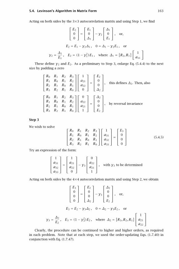
5.4. Levinson’s Algorithm in Matrix Form 163
Acting on both sides by the 3×3 autocorrelation matrix and using Step 1, we find⎡⎢⎣ E2
00
⎤⎥⎦ =⎡⎢⎣ E1
0Δ1
⎤⎥⎦− γ2
⎡⎢⎣Δ1
0E1
⎤⎥⎦ , or,
E2 = E1 − γ2Δ1 , 0 = Δ1 − γ2E1 , or
γ2 = Δ1
E1, E2 = (1− γ2
1)E1 , where Δ1 =[R2, R1
][1a11
]These define γ2 and E2. As a preliminary to Step 3, enlarge Eq. (5.4.4) to the next
size by padding a zero⎡⎢⎢⎢⎣R0 R1 R2 R3
R1 R0 R1 R2
R2 R1 R0 R1
R3 R2 R1 R0
⎤⎥⎥⎥⎦⎡⎢⎢⎢⎣
1a21
a22
0
⎤⎥⎥⎥⎦ =⎡⎢⎢⎢⎣E2
00Δ2
⎤⎥⎥⎥⎦ , this defines Δ2. Then, also
⎡⎢⎢⎢⎣R0 R1 R2 R3
R1 R0 R1 R2
R2 R1 R0 R1
R3 R2 R1 R0
⎤⎥⎥⎥⎦⎡⎢⎢⎢⎣
0a22
a21
1
⎤⎥⎥⎥⎦ =⎡⎢⎢⎢⎣Δ2
00E2
⎤⎥⎥⎥⎦ , by reversal invariance
Step 3
We wish to solve ⎡⎢⎢⎢⎣R0 R1 R2 R3
R1 R0 R1 R2
R2 R1 R0 R1
R3 R2 R1 R0
⎤⎥⎥⎥⎦⎡⎢⎢⎢⎣
1a31
a32
a33
⎤⎥⎥⎥⎦ =⎡⎢⎢⎢⎣E3
000
⎤⎥⎥⎥⎦ (5.4.5)
Try an expression of the form:⎡⎢⎢⎢⎣1a31
a32
a33
⎤⎥⎥⎥⎦ =⎡⎢⎢⎢⎣
1a21
a22
0
⎤⎥⎥⎥⎦− γ3
⎡⎢⎢⎢⎣0a22
a21
1
⎤⎥⎥⎥⎦ , with γ3 to be determined
Acting on both sides by the 4×4 autocorrelation matrix and using Step 2, we obtain⎡⎢⎢⎢⎣E3
000
⎤⎥⎥⎥⎦ =⎡⎢⎢⎢⎣E2
00Δ2
⎤⎥⎥⎥⎦− γ3
⎡⎢⎢⎢⎣Δ2
00E2
⎤⎥⎥⎥⎦ , or,
E3 = E2 − γ3Δ2 , 0 = Δ2 − γ3E2 , or
γ3 = Δ2
E2, E3 = (1− γ2
3)E2 , where Δ2 =[R3, R2, R1
]⎡⎢⎣ 1a21
a22
⎤⎥⎦Clearly, the procedure can be continued to higher and higher orders, as required
in each problem. Note that at each step, we used the order-updating Eqs. (1.7.40) inconjunction with Eq. (1.7.47).

164 5. Linear Prediction
5.5 Autocorrelation Sequence Extensions
In this section, we discuss the problem of extending an autocorrelation function andthe related issues of singular autocorrelation matrices. The equivalence between anautocorrelation function and the set of reflection coefficients provides a convenient andsystematic way to (a) test whether a given finite set of numbers are the autocorrelationlags of a stationary signal and (b) extend a given finite set of autocorrelation lags toarbitrary lengths while preserving the autocorrelation property.
For a finite set of numbers {R(0),R(1), . . . , R(p)} to be the lags of an autocorre-lation function, it is necessary and sufficient that all reflection coefficients, extractedfrom this set via the Levinson recursion, have magnitude less than one; that is, |γi| < 1,for i = 1,2, . . . , p, and also that R(0)> 0. These conditions are equivalent to the pos-itive definiteness of the autocorrelation matrix Rp. The proof follows from the factthat the positivity of Rp is equivalent to the conditions on the prediction errors Ei > 0,for i = 1,2, . . . , p. In turn, these conditions are equivalent to E0 = R(0)> 0 and and,through Eq. (5.3.13), to the reflection coefficients having magnitude less than one.
The problem of extending a finite set {R(0),R(1), . . . , R(p)} of autocorrelation lagsis to find a numberR(p+1) such that the extended set {R(0),R(1), . . . , R(p),R(p+1)}is still an autocorrelation sequence. This can be done by parametrizing R(p + 1) interms of the next reflection coefficient γp+1. Solving Eq. (5.3.12) for R(p+1) and usingEq. (5.3.11), we obtain
R(p+ 1)= γp+1Ep −[ap1R(p)+ap2R(p− 1)+· · · + appR(1)
](5.5.1)
Any number γp+1 in the range−1 < γp+1 < 1 will give rise to an acceptable value forR(p+1) . The choiceγp+1 = 0 is special and corresponds to the so-called autoregressiveor maximum entropy extension of the autocorrelation function (see Problem 5.16). If thischoice is repeated to infinity, we will obtain the set of reflection coefficients
{γ1, γ2, . . . , γp,0,0, . . . }
It follows from the Levinson recursion that all prediction-error filters of order greaterthan p will remain equal to the pth filter,Ap(z)= Ap+1(z)= Ap+2(z)= · · · . Therefore,the corresponding whitening filter will beA(z)= Ap(z), that is, an autoregressive modelof order p. With the exception of the above autoregressive extension that leads to anall-pole signal model, the extendibility conditions |γp+i| < 1, i ≥ 1, do not necessarilyguarantee that the resulting signal model will be a rational (pole-zero) model. See [16-20]for some recent results on this subject.
Example 5.5.1: Consider the three numbers {R(0),R(1),R(2)} = {8,4,−1}. The Levinsonrecursion gives {γ1, γ2} = {0.5,−0.5} and {E1, E2} = {6, 4.5}. Thus, the above numbersqualify to be autocorrelation lags. The corresponding prediction-error filters are
a1 =[
1a11
]=
[1−0.5
], a2 =
⎡⎢⎣ 1a21
a22
⎤⎥⎦ =⎡⎢⎣ 1−0.75
0.5
⎤⎥⎦The next lag in this sequence can be chosen according to Eq. (5.5.1)
R(3)= γ3E2 −[a21R(2)+a22R(1)
] = 4.5γ3 − 2.75
where γ3 is any number in the interval −1 < γ3 < 1 . The resulting possible values ofR(3) are plotted below versus γ3 . In particular, the autoregressive extension correspondsto γ3 = 0, which gives R(3)= −2.75. ��

5.5. Autocorrelation Sequence Extensions 165
The end-points, γp+1 = ±1, of the allowed interval (−1,1) correspond to the twopossible extreme values of R(p+ 1):
R(p+ 1)= ±Ep −[ap1R(p)+ap2R(p− 1)+· · · + appR(1)
]In this case, the corresponding prediction error vanishes Ep+1 = (1− γ2
p+1)Ep = 0.This makes the resulting order-(p+ 1) autocorrelation matrix Rp+1 singular. The pre-diction filter becomes either the symmetric (if γp+1 = −1) or antisymmetric (if γp+1 = 1)combination
ap+1 =[
ap0
]+
[0aRp
], Ap+1(z)= Ap(z)+z−1ARp(z) , or,
ap+1 =[
ap0
]−
[0aRp
], Ap+1(z)= Ap(z)−z−1ARp(z)
In either case, it can be shown that the zeros of the polynomial Ap+1(z) lie onthe unit circle, and that the prediction filter ap+1 becomes an eigenvector of Rp+1 withzero eigenvalue; namely, Rp+1ap+1 = 0. This follows from the normal Eqs. (5.3.28)Rp+1ap+1 = Ep+1up+1 and Ep+1 = 0.
Example 5.5.2: Consider the extended autocorrelation sequence of Example 5.5.1 defined bythe singular choice γ3 = −1. Then, R(3)= −4.5 − 2.75 = −7.25. The correspondingorder-3 prediction-error filter is computed using the order-2 predictor and the Levinsonrecursion
a3 =
⎡⎢⎢⎢⎣1a31
a32
a33
⎤⎥⎥⎥⎦ =⎡⎢⎢⎢⎣
1−0.75
0.50
⎤⎥⎥⎥⎦− γ3
⎡⎢⎢⎢⎣0
0.5−0.75
1
⎤⎥⎥⎥⎦ =⎡⎢⎢⎢⎣
1−0.25−0.25
1
⎤⎥⎥⎥⎦It is symmetric about its middle. Its zeros, computed as the solutions of (1 − 0.25z−1 −0.25z−2 + z−3)= (1+ z−1)(1− 1.25z−1 + z−2)= 0 are
z = −1 , z = 5± j√39
8
and lie on the unit circle. Finally, we verify that a3 is an eigenvector of R3 with zeroeigenvalue:
R3a3 =
⎡⎢⎢⎢⎣8 4 −1 −7.254 8 4 −1−1 4 8 4−7.25 −1 4 8
⎤⎥⎥⎥⎦⎡⎢⎢⎢⎣
1−0.25−0.25
1
⎤⎥⎥⎥⎦ = 0 ��
Singular autocorrelation matrices, and the associated symmetric or antisymmetricprediction filters with zeros on the unit circle, find application in the method of linespectrum pairs (LSP) of speech analysis [21]. They are also intimately related to theeigenvector methods of spectrum estimation, such as Pisarenko’s method of harmonicretrieval, discussed in Section 6.2. This connection arises from the property that singular

166 5. Linear Prediction
autocorrelation matrices (with nonsingular principal minors) admit a representation asa sum of sinusoidal components [22], the frequencies of which are given precisely bythe zeros, on the unit circle, of the corresponding prediction filter. This sinusoidalrepresentation is equivalent to the eigen-decomposition of the matrix. The predictionfilter can, alternatively, be computed as the eigenvector belonging to zero eigenvalue.The proof of these results can be derived as a limiting case; namely, the noise-free case,of the more general eigenvector methods that deal with sinusoids in noise. A directproof is suggested in Problem 6.10.
Example 5.5.3: Consider the autocorrelation matrix R =⎡⎢⎣ 2 1 −1
1 2 1−1 1 2
⎤⎥⎦. It is easily verified
that the corresponding autocorrelation lags R(k) admit the sinusoidal representation
R(k)= 2 cos(ω1k)= ejω1k + e−jω1k , for k = 0,1,2
where ω1 = π/3. Sending these lags through the Levinson recursion, we find {γ1, γ2} ={0.5,−1} and {E1, E2} = {1.5, 0}. Thus, R singular. Its eigenvalues are {0, 3, 3}. Thecorresponding prediction filters are a1 = [1,−0.5]T and a2 = [1,−1,1]T . It is easilyverified that a2 is an eigenvector ofRwith zero eigenvalue, i.e.,Ra2 = 0. The correspondingeigenfilter A2(z)= 1 − z−1 + z−2, is symmetric about its middle and has zeros on theunit circle coinciding with the sinusoids present in R, namely, z = e±jω1 . The other twoeigenvectors of R are
c =⎡⎢⎣ 1
cosω1
cos 2ω1
⎤⎥⎦ =⎡⎢⎣ 1
0.5−0.5
⎤⎥⎦ , d =⎡⎢⎣ 0
sinω1
sin 2ω1
⎤⎥⎦ =⎡⎢⎣ 0√
3/2√3/2
⎤⎥⎦both belonging to eigenvalue λ = 3. Their norm is ‖c‖ = ‖d‖ = √3/2. The three eigen-vectors a2, c,d are mutually orthogonal. It is easily verified that the matrix R may be rep-resented in the form R = 2ccT + 2ddT , which, after normalizing c and d to unit norm, isrecognized as the eigendecomposition of R, We can also express R in terms of its complexsinusoidal components in the form R = ss† + s∗sT , where
s = c+ jd =⎡⎢⎣ 1ejω1
e2jω1
⎤⎥⎦ , s† = s∗T = [1, e−jω1 , e−2jω1
]
Example 5.5.4: Similarly, one can verify that the four autocorrelation lags {8, 4, −1, −7.25} ofthe singular matrix of Example 5.5.2 can be represented in the sinusoidal form
R(k)= P1ejω1k + P2ejω2k + P3ejω3k , for k = 0,1,2,3
where P1 = 8/13, P2 = P3 = 96/13, and ωi correspond to the zeros of the predictionfilter a3, namely,
ejω1 = −1 , ejω2 = 5+ j√39
8, ejω3 = 5− j√39
8, so that,ω3 = −ω2
The matrix itself has the sinusoidal representation
R = P1s1s†1 + P2s2s†2 + P3s3s†3 , where si =
⎡⎢⎢⎢⎣1ejωie2jωi
e3jωi
⎤⎥⎥⎥⎦Had we chosen the value γ3 = 1 in Example 5.5.2, we would have found the extended lagR(3)= 1.75 and the antisymmetric order-3 prediction-error filter a3 = [1,−1.25,1.25,−1]T ,whose zeros are on the unit circle:
ejω1 = 1 , ejω2 = 1+ j√63
8, ejω3 = 1− j√63
8

5.6. Split Levinson Algorithm 167
with R(k) admitting the sinusoidal representation
R(k)= P1 + 2P2 cos(ω2k)= [8, 4, −1, 1.75] , for k = 0,1,2,3
where P1 = 24/7 and P2 = 16/7. ��
5.6 Split Levinson Algorithm
The main computational burden of Levinson’s algorithm is 2pmultiplications per stage,arising from the p multiplications in Eq. (5.3.15) and in the computation of the innerproduct (5.3.12). Thus, forM stages, the algorithm requires
2M∑p=1
p =M(M + 1)
or,O(M2)multiplications. This represents a factor ofM savings over solving the normalequations (5.3.7) by direct matrix inversion, requiring O(M3) operations. The savingscan be substantial considering that in speech processing M = 10–15, and in seismicprocessingM = 100–200. Progress in VLSI hardware has motivated the development ofefficient parallel implementations of Levinson’s algorithm and its variants [23–42]. WithM parallel processors, the complexity of the algorithm is typically reduced by anotherfactor ofM to O(M) or O(M logM) operations.
An interesting recent development is the realization that Levinson’s algorithm hassome inherent redundancy, which can be exploited to derive more efficient versionsof the algorithm allowing an additional 50% reduction in computational complexity.These versions were motivated by a new stability test for linear prediction polynomialsby Bistritz [43], and have been termed Split Levinson or Immitance-Domain Levinsonalgorithms [44–51]. They are based on efficient three-term recurrence relations for thesymmetrized or antisymmetrized prediction polynomials. Following [44], we define theorder-p symmetric polynomial
Fp(z)= Ap−1(z)+z−1ARp−1(z) , fp =[
ap−1
0
]+
[0
aRp−1
](5.6.1)
The coefficient vector fp is symmetric about its middle; that is, fp0 = fpp = 1 andfpi = ap−1,i+ap−1,p−i = fp,p−i, for i = 1,2, . . . , p− 1. Thus, only half of the vector fp, isneeded to specify it completely. Using the backward recursion (5.3.22) to writeAp−1(z)in terms of Ap(z), we obtain the alternative expression
Fp = 1
1− γ2p
[(Ap + γpARp)+z−1(γpzAp + zARp)
] = 1
1− γp [Ap +ARp] , or,
(1− γp)Fp(z)= Ap(z)+ARp(z) , (1− γp)fp = ap + aRp (5.6.2)
The polynomial Ap(z) and its reverse may be recovered from the knowledge of thesymmetric polynomials Fp(z). Writing Eq. (5.6.1) for order p+ 1, we obtain Fp+1(z)=Ap(z)+z−1ARp(z). This equation, together with Eq. (5.6.2), may be solved for Ap(z)and ARp(z), yielding
Ap(z)= Fp+1(z)−(1− γp)z−1Fp(z)1− z−1
, ARp(z)=(1− γp)Fp(z)−Fp+1(z)
1− z−1(5.6.3)
Inserting these expressions into the forward Levinson recursion (5.3.16) and can-celing the common factor 1/(1 − z−1), we obtain a three-term recurrence relation forFp(z):
Fp+2 − (1− γp+1)z−1Fp+1 =[Fp+1 − (1− γp)z−1Fp
]− γp+1z−1[(1− γp)Fp − Fp+1]
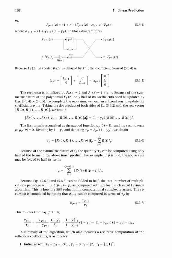
168 5. Linear Prediction
or,Fp+2(z)= (1+ z−1)Fp+1(z)−αp+1z−1Fp(z) (5.6.4)
where αp+1 = (1+ γp+1)(1− γp). In block diagram form
Because Fp(z) has order p and is delayed by z−1, the coefficient form of (5.6.4) is
fp+2 =[
fp+1
0
]+
[0
fp+1
]−αp+1
⎡⎢⎣ 0fp0
⎤⎥⎦ (5.6.5)
The recursion is initialized by F0(z)= 2 and F1(z)= 1 + z−1. Because of the sym-metric nature of the polynomial Fp(z) only half of its coefficients need be updated byEqs. (5.6.4) or (5.6.5). To complete the recursion, we need an efficient way to update thecoefficientsαp+1. Taking the dot product of both sides of Eq. (5.6.2) with the row vector[R(0),R(1), . . . , R(p)
], we obtain[
R(0), . . . , R(p)]ap +
[R(0), . . . , R(p)
]aRp = (1− γp)
[R(0), . . . , R(p)
]fp
The first term is recognized as the gapped function gp(0)= Ep, and the second termas gp(p)= 0. Dividing by 1− γp and denoting τp = Ep/(1− γp), we obtain
τp =[R(0),R(1), . . . , R(p)
]fp =
p∑i=0
R(i)fpi (5.6.6)
Because of the symmetric nature of fp the quantity τp can be computed using onlyhalf of the terms in the above inner product. For example, if p is odd, the above summay be folded to half its terms
τp =(p−1)/2∑i=0
[R(i)+R(p− i)]fpi
Because Eqs. (5.6.5) and (5.6.6) can be folded in half, the total number of multipli-cations per stage will be 2(p/2)= p, as compared with 2p for the classical Levinsonalgorithm. This is how the 50% reduction in computational complexity arises. The re-cursion is completed by noting that αp+1 can be computed in terms of τp by
αp+1 = τp+1
τp(5.6.7)
This follows from Eq. (5.3.13),
τp+1
τp= Ep+1
1− γp+1
1− γpEp
= 1− γ2p+1
1− γp+1(1− γp)= (1+ γp+1)(1− γp)= αp+1
A summary of the algorithm, which also includes a recursive computation of thereflection coefficients, is as follows:
1. Initialize with τ0 = E0 = R(0), γ0 = 0, f0 = [2], f1 = [1,1]T.

5.6. Split Levinson Algorithm 169
2. At stage p, the quantities τp,γp, fp, fp+1 are available.
3. Compute τp+1 from Eq. (5.6.6), using only half the terms in the sum.
4. Compute αp+1 from Eq. (5.6.7), and solve for γp+1 = −1+αp+1/(1− γp).5. Compute fp+2 from Eq. (5.6.5), using half of the coefficients.
6. Go to stage p+ 1.
After the final desired order is reached, the linear prediction polynomial can berecovered from Eq. (5.6.3), which can be written recursively as
api = ap,i−1 + fp+1.i − (1− γp)fp,i−1 , i = 1,2, . . . , p (5.6.8)
with ap0 = 1, or vectorially,[ap0
]=
[0ap
]+ fp+1 − (1− γp)
[0fp
](5.6.9)
Using the three-term recurrence (5.6.5), we may replace fp+1 in terms of fp and fp−1,and rewrite Eq. (5.6.9) as
[ap0
]=
[0ap
]+
[fp0
]+ γp
[0fp
]−αp
⎡⎢⎣ 0fp−1
0
⎤⎥⎦ (5.6.10)
and in the z-domain
Ap(z)= z−1Ap(z)+(1+ γpz−1)Fp(z)−αpz−1Fp−1(z) (5.6.11)
Example 5.6.1: We rederive the results of Example 5.3.1 using this algorithm, showing explicitlythe computational savings. Initialize with τ0 = R(0)= 128, f0 = [2], f1 = [1,1]T . Using(5.6.6), we compute
τ1 =[R(0),R(1)
]f1 =
[R(0)+R(1)]f10 = 128− 64 = 64
Thus, α1 = τ1/τ0 = 64/128 = 0.5 and γ1 = −1+α1 = −0.5. Using Eq. (5.6.5) we find
f2 =[
f1
0
]+
[0f1
]−α1
⎡⎢⎣ 0f0
0
⎤⎥⎦ =⎡⎢⎣ 1
10
⎤⎥⎦+⎡⎢⎣ 0
11
⎤⎥⎦− 0.5
⎡⎢⎣ 020
⎤⎥⎦ =⎡⎢⎣ 1
11
⎤⎥⎦and compute τ2
τ2 =[R(0),R(1),R(2)
]f2 =
[R(0)+R(2)]f20 +R(1)f21 = 144
Thus, α2 = τ2/τ1 = 144/64 = 2.25 and γ2 = −1 +α2/(1 − γ1)= −1 + 2.25/1.5 = 0.5.Next, compute f3 and τ3
f3 =[
f2
0
]+
[0f2
]−α2
⎡⎢⎣ 0f1
0
⎤⎥⎦ =⎡⎢⎢⎢⎣
1110
⎤⎥⎥⎥⎦+⎡⎢⎢⎢⎣
0111
⎤⎥⎥⎥⎦− 2.25
⎡⎢⎢⎢⎣0110
⎤⎥⎥⎥⎦ =⎡⎢⎢⎢⎣
1−0.25−0.25
1
⎤⎥⎥⎥⎦τ3 =
[R(0),R(1),R(2),R(3)
]f3 =
[R(0)+R(3)]f30 +
[R(1)+R(2)]f31 = 36
which gives α3 = τ3/τ2 = 36/144 = 0.25 and γ3 = −1 +α3/(1 − γ2)= −0.5. Next, wecompute f4 and τ4
f4 =[
f3
0
]+
[0f3
]−α3
⎡⎢⎣ 0f2
0
⎤⎥⎦ =⎡⎢⎢⎢⎢⎢⎢⎣
1−0.25−0.25
10
⎤⎥⎥⎥⎥⎥⎥⎦+⎡⎢⎢⎢⎢⎢⎢⎣
01
−0.25−0.25
1
⎤⎥⎥⎥⎥⎥⎥⎦− 0.25
⎡⎢⎢⎢⎢⎢⎢⎣01110
⎤⎥⎥⎥⎥⎥⎥⎦ =⎡⎢⎢⎢⎢⎢⎢⎣
10.5−0.75
0.51
⎤⎥⎥⎥⎥⎥⎥⎦

170 5. Linear Prediction
τ4 =[R(0),R(1),R(2),R(3),R(4)
]f4
= [R(0)+R(4)]f40 +
[R(1)+R(3)]f41 +R(2)f42 = 81
which gives α4 = τ4/τ3 = 81/36 = 2.25 and γ4 = −1 + α4/(1 − γ3)= 0.5. The finalprediction filter a4 can be computed using Eq. (5.6.9) or (5.6.10). To avoid computing f5
we use Eq. (5.6.10), which gives⎡⎢⎢⎢⎢⎢⎢⎢⎢⎣
1a41
a42
a43
a44
0
⎤⎥⎥⎥⎥⎥⎥⎥⎥⎦=
⎡⎢⎢⎢⎢⎢⎢⎢⎢⎣
01a41
a42
a43
a44
⎤⎥⎥⎥⎥⎥⎥⎥⎥⎦+
⎡⎢⎢⎢⎢⎢⎢⎢⎢⎣
10.5−0.75
0.510
⎤⎥⎥⎥⎥⎥⎥⎥⎥⎦+ 0.5
⎡⎢⎢⎢⎢⎢⎢⎢⎢⎣
01
0.5−0.75
0.51
⎤⎥⎥⎥⎥⎥⎥⎥⎥⎦− 2.25
⎡⎢⎢⎢⎢⎢⎢⎢⎢⎣
01
−0.25−0.25
10
⎤⎥⎥⎥⎥⎥⎥⎥⎥⎦with solution a4 = [1, −0.25, −0.1875, 0.5, −0.5]T . ��
5.7 Analysis and Synthesis Lattice Filters
The Levinson recursion, expressed in the 2×2 matrix form of Eq. (5.3.18) forms the basisof the so-called lattice, or ladder, realizations of the prediction-error filters and theirinverses [3,6]. Remembering that the prediction-error sequence ep(n) is the convolutionof the prediction-error filter [1, ap1, ap2, . . . , app] with the original data sequence yn,that is,
e+p (n)= yn + ap1yn−1 + ap2yn−2 + · · · + appyn−p (5.7.1)
we find in the z-domainE+p (z)= Ap(z)Y(z) (5.7.2)
where we changed the notation slightly and denoted ep(n) by e+p (n). At this point,it proves convenient to introduce the backward prediction-error sequence, defined interms of the reverse of the prediction-error filter, as follows:
E−p (z) = ARp(z)Y(z) (5.7.3)
e−p (n) = yn−p + ap1yn−p+1 + ap2yn−p+2 + · · · + appyn (5.7.4)
where ARp(z) is the reverse of Ap(z), namely,
ARp(z)= z−pAp(z−1)= app + ap,p−1z−1 + ap,p−2z−2 + · · · + ap1z−(p−1) + z−p
The signal sequence e−p (n)may be interpreted as the postdiction error in postdictingthe value of yn−p on the basis of the future p samples {yn−p+1, yn−p+2, . . . , yn−1, yn},as shown below
Actually, the above choice of postdiction coefficients is the optimal one that mini-mizes the mean-square postdiction error
E[e−p (n)2]= min (5.7.5)

5.7. Analysis and Synthesis Lattice Filters 171
This is easily shown by inserting Eq. (5.7.4) into (5.7.5) and using stationarity
E[e−p (n)2] = E⎡⎢⎣⎛⎝ p∑m=0
apmyn−p+m
⎞⎠2⎤⎥⎦ = p∑
m,k=0
apmE[yn−p+myn−p+k]apk
=p∑
m,k=0
apmR(m− k)apk = E[e+p (n)2]
which shows that the forward and the backward prediction error criteria are the same,thus, having the same solution for the optimal coefficients. We can write Eqs. (5.7.1) and(5.7.4) vectorially
e+p (n)= [1, ap1, . . . , app]
⎡⎢⎢⎢⎢⎢⎣ynyn−1
...yn−p
⎤⎥⎥⎥⎥⎥⎦ = aTpyp(n) (5.7.6a)
e−p (n)= [app, ap,p−1, . . . ,1]
⎡⎢⎢⎢⎢⎢⎣ynyn−1
...yn−p
⎤⎥⎥⎥⎥⎥⎦ = aRTp yp(n)= bTpyp(n) (5.7.6b)
They are recognized as the forward and backward prediction errors ea and eb ofEq. (1.7.9). Multiplying both sides of the Levinson recursion (5.3.18) by Y(z), we cast itin the equivalent form in terms of the forward and backward prediction-error sequences:[
E+p+1(z)E−p+1(z)
]=
[1 −γp+1z−1
−γp+1 z−1
][E+p (z)E−p (z)
](5.7.7)
and in the time domain
e+p+1(n) = e+p (n)−γp+1e−p (n− 1)
e−p+1(n) = e−p (n− 1)−γp+1e+p (n)(5.7.8)
and in block diagram form
These recursions are initialized at p = 0 by
E±0 (z)= A0(z)Y(z)= Y(z) and e±0 (n)= yn (5.7.9)
Eqs. (5.7.8) are identical to (1.7.50), with the identifications ea → e+p+1(n), ea →e+p (n), eb → e−p+1(n), eb → e−p (n− 1) the last following from Eq. (5.3.26).
The lattice realization of the prediction-error filter is based on the recursion (5.7.8).Starting at p = 0, the output of the pth stage of (5.7.8) becomes the input of the (p+1)thstage, up to the final desired order p =M. This is depicted in Fig. 5.3.
At each time instant n the numbers held in the M delay registers of the lattice canbe taken as the internal state of the lattice. The subroutine lattice (see Appendix B) isan implementation of Fig. 5.3. At each instant n, the routine takes two overall inputs

172 5. Linear Prediction
Fig. 5.3 Analysis lattice filter.
e±0 (n), makes M calls to the routine section that implements the single lattice section(5.7.8), produces the two overall outputs e±M(n), and updates the internal state of thelattice in preparation for the next call. By allowing the reflection coefficients to changebetween calls, the routine can also be used in adaptive lattice filters.
Equations (5.7.2) and (5.7.3) imply that the transfer function from the input yn to theoutput e+M(n) is the desired prediction-error filter AM(z), whereas the transfer func-tion from yn to e−M(n) is the reversed filter ARM(z). The lattice realization is thereforeequivalent to the direct-form realization
e+M(n)= yn + aM1yn−1 + aM2yn−2 + · · ·aMMyn−M
realized directly in terms of the prediction coefficients. It is depicted below
The synthesis filter 1/AM(z) can also be realized in a lattice form. The input tothe synthesis filter is the prediction error sequence e+M(n) and its output is the originalsequence yn :
Its direct-form realization is:
For the lattice realization, since yn corresponds to e+0 (n), we must write Eq. (5.7.8) inan order-decreasing form, starting at e+M(n) and ending with e+0 (n)= yn. Rearranging

5.7. Analysis and Synthesis Lattice Filters 173
the terms of the first of Eqs. (5.7.8), we have
e+p (n) = e+p+1(n)+γp+1e−p (n− 1)
e−p+1(n) = e−p (n− 1)−γp+1e+p (n)(5.7.10)
which can be realized as shown below:
Note the difference in signs in the upper and lower adders. Putting together thestages from p =M to p = 0, we obtain the synthesis lattice filter shown in Fig. 5.4.
Fig. 5.4 Synthesis lattice filter.
Lattice structures based on the split Levinson algorithm can also be developed [46, 47].They are obtained by cascading the block diagram realizations of Eq. (5.6.4) for differentvalues of αp. The output signals from each section are defined by
ep(n)=p∑i=0
fpiyn−i , Ep(z)= Fp(z)Y(z)
Multiplying both sides of Eq. (5.6.1) by Y(z) we obtain the time-domain expression
ep(n)= e+p−1(n)+e−p−1(n− 1)
Similarly, multiplying both sides of Eq. (5.6.4) by Y(z) we obtain the recursions
ep+2(n)= ep+1(n)+ep+1(n− 1)−αpep(n− 1)
They are initialized by e0(n)= 2yn and e1(n)= yn + yn−1. Putting together thevarious sections we obtain the lattice-type realization
The forward prediction error may be recovered from Eq. (5.6.3) or (5.6.11) by multi-plying both sides with Y(z); for example, using Eq. (5.6.11) we find
e+p (n)= e+p−1(n)+ep(n)+γpep(n)−αpep−1(n− 1)

174 5. Linear Prediction
5.8 Alternative Proof of the Minimum-Phase Property
The synthesis filter 1/AM(z) must be stable and causal, which requires all theM zerosof the prediction-error filter AM(z) to lie inside the unit circle on the complex z-plane.We have already presented a proof of this fact which was based on the property thatthe coefficients of AM(z) minimized the mean-squared prediction error E[e+M(n)2].Here, we present an alternative proof based on the Levinson recursion and the fact thatall reflection coefficients γp have magnitude less than one [6,11]. From the definition(5.7.4), it follows that
e−p (n− 1)= yn−p−1 + ap1yn−p + ap2yn−p+1 + · · · + appyn−1 (5.8.1)
This quantity represents the estimation error of postdicting yn−p−1 on the basis of thep future samples {yn−p, yn−p+1, . . . , yn−1}. Another way to say this is that the linearcombination of these p samples is the projection of yn−p−1 onto the subspace of randomvariables spanned by {yn−p, yn−p+1, . . . , yn−1}; that is,
e−p (n− 1)= yn−p−1 − (projection of yn−p−1 onto {yn−p, yn−p+1, . . . , yn−1}) (5.8.2)
On the other hand, e+p (n) given in Eq. (5.7.1) is the estimation error of yn based onthe same set of samples. Therefore,
e+p (n)= yn − (projection of yn onto {yn−p, yn−p+1, . . . , yn−1}) (5.8.3)
The samples {yn−p, yn−p+1, . . . , yn−1} are the intermediate set of samples between yn−p−1
and yn as shown below:
Therefore, according to the discussion in Section 1.6, the PARCOR coefficient be-tween yn−p−1 and yn with the effect of intermediate samples removed is given by
PARCOR = E[e+p (n)e−p (n− 1)
]E[e−p (n− 1)2
]This is precisely the reflection coefficient γp+1 of Eq. (5.3.11). Indeed, using Eq. (5.8.1)and the gap conditions, gp(k)= 0, k = 1,2, . . . , p, we find
E[e+p (n)e−p (n− 1)
] = E[e+p (n)(yn−p−1 + ap1yn−p + ap2yn−p+1 + · · · + appyn−1)
]= gp(p+ 1)+ap1gp(p)+ap2gp(p− 1)+· · ·appgp(1)= gp(p+ 1)
Similarly, invoking stationarity and Eq. (5.7.5),
E[e−p (n− 1)2] = E[
e−p (n)2] = E[e+p (n)2] = gp(0)
Thus, the reflection coefficient γp+1 is really a PARCOR coefficient:
γp+1 =E[e+p (n)e−p (n− 1)
]E[e−p (n− 1)2
] = E[e+p (n)e−p (n− 1)
]√E[e−p (n− 1)2
]E[e+p (n)2
] (5.8.4)
Using the Schwarz inequality with respect to the inner product E[uv], that is,∣∣E[uv]∣∣2 ≤ E[u2]E[v2]

5.8. Alternative Proof of the Minimum-Phase Property 175
then Eq. (5.8.4) implies that γp+1 will have magnitude less than one:
|γp+1| ≤ 1 , for each p = 0,1, . . . (5.8.5)
To prove the minimum-phase property of AM(z) we must show that all of its Mzeros are inside the unit circle. We will do this by induction. Let Zp and Np denotethe number of zeros and poles of Ap(z) that lie inside the unit circle. Levinson’s re-cursion, Eq. (5.3.13), expresses Ap+1(z) as the sum of Ap(z) and a correction termF(z)= −γp+1z−1ARp(z), that is,
Ap+1(z)= Ap(z)+F(z)
Using the inequality (5.8.5) and the fact that Ap(z) has the same magnitude spectrumas ARp(z), we find the inequality∣∣F(z)∣∣ = ∣∣−γp+1z−1ARp(z)
∣∣ = ∣∣γp+1Ap(z)∣∣ ≤ ∣∣Ap(z)∣∣
for z = ejω on the unit circle. Then, the argument principle and Rouche’s theorem implythat the addition of the function F(z) will not affect the difference Np − Zp of polesand zeros contained inside the unit circle. Thus,
Np+1 − Zp+1 = Np − ZpSince the only pole of Ap(z) is the multiple pole of order p at the origin arising fromthe term z−p, it follows that Np = p. Therefore,
(p+ 1)−Zp+1 = p− Zp , or,
Zp+1 = Zp + 1
Starting at p = 0 with A0(z)= 1, we have Z0 = 0. It follows that
Zp = p
which states that all the p zeros of the polynomial Ap(z) lie inside the unit circle.Another way to state this result is: “A necessary and sufficient condition for a poly-
nomialAM(z) to have all of itsM zeros strictly inside the unit circle is that all reflectioncoefficients {γ1, γ2, . . . , γM} resulting from AM(z) via the backward recursion (5.3.21)have magnitude strictly less than one.” This is essentially equivalent to the well-knownSchur-Cohn test of stability [52–56]. The subroutine bkwlev can be used in this regardto obtain the sequence of reflection coefficients. The Bistritz test [43], mentioned inSection 5.6, is an alternative stability test.
Example 5.8.1: Test the minimum phase property of the polynomials
(a) A(z)= 1− 2.60z−1 + 2.55z−2 − 2.80z−3 + 0.50z−4
(b) A(z)= 1− 1.40z−1 + 1.47z−2 − 1.30z−3 + 0.50z−4
Sending the coefficients of each through the subroutine bkwlev, we find the set of reflec-tion coefficients
(a) {0.4,−0.5,2.0,−0.5}(b) {0.4,−0.5,0.8,−0.5}
Since among (a) there is one reflection coefficient of magnitude greater than one, case (a)will not be minimum phase, whereas case (b) is. ��

176 5. Linear Prediction
5.9 Orthogonality of Backward Prediction Errors—Cholesky
Factorization
Another interesting structural property of the lattice realizations is that, in a certainsense, the backward prediction errors e−p (n) are orthogonal to each other [3,6]. To seethis, consider the caseM = 3, and form the matrix product⎡⎢⎢⎢⎣
R0 R1 R2 R3
R1 R0 R1 R2
R2 R1 R0 R1
R3 R2 R1 R0
⎤⎥⎥⎥⎦︸ ︷︷ ︸
R
⎡⎢⎢⎢⎣1 a11 a22 a33
0 1 a21 a32
0 0 1 a31
0 0 0 1
⎤⎥⎥⎥⎦︸ ︷︷ ︸
LT
=
⎡⎢⎢⎢⎣E0 0 0 0∗ E1 0 0∗ ∗ E2 0∗ ∗ ∗ E3
⎤⎥⎥⎥⎦︸ ︷︷ ︸
L1
Because the normal equations (written upside down) are satisfied by each prediction-error filter, the right-hand side will be a lower-triangular matrix. The “don’t care” entrieshave been denoted by ∗s. Multiply from the left by L to get
LRLT = LL1 =
⎡⎢⎢⎢⎣E0 0 0 0∗ E1 0 0∗ ∗ E2 0∗ ∗ ∗ E3
⎤⎥⎥⎥⎦Since L is by definition lower-triangular, the right-hand side will still be lower tri-
angular. But the left-hand side is symmetric. Thus, so is the right-hand side and as aresult it must be diagonal. We have shown that
LRLT = D = diag{E0, E1, E2, E3} (5.9.1)
or, written explicitly⎡⎢⎢⎢⎣1 0 0 0a11 1 0 0a22 a21 1 0a33 a32 a31 1
⎤⎥⎥⎥⎦⎡⎢⎢⎢⎣R0 R1 R2 R3
R1 R0 R1 R2
R2 R1 R0 R1
R3 R2 R1 R0
⎤⎥⎥⎥⎦⎡⎢⎢⎢⎣
1 a11 a22 a33
0 1 a21 a32
0 0 1 a31
0 0 0 1
⎤⎥⎥⎥⎦=⎡⎢⎢⎢⎣E0 0 0 00 E1 0 00 0 E2 00 0 0 E3
⎤⎥⎥⎥⎦This is identical to Eq. (1.7.17). The pqth element of this matrix equation is then
bTpRbq = δpqEp (5.9.2)
where bp and bq denote the pth and qth columns of LT. These are recognized as thebackward prediction-error filters of orders p and q. Eq. (5.9.2) implies then the orthog-onality of the backward prediction-error filters with respect to an inner product xTRy.
The backward prediction errors e−p (n) can be expressed in terms of the bps and thevector of samples y(n)= [yn, yn−1, yn−2, yn−3]T, as follows:
e−0 (n)= [1, 0, 0, 0]y(n)= bT0 y(n)= yne−1 (n)= [a11, 1, 0, 0]y(n)= bT1 y(n)= a11yn + yn−1
e−2 (n)= [a22, a21, 1, 0]y(n)= bT2 y(n)= a22yn + a21yn−1 + yn−2
e−3 (n)= [a33, a32, a31,1]y(n)= bT3 y(n)= a33yn + a32yn−1 + a31yn−2 + yn−3
(5.9.3)
which can be rearranged into the vector form
e−(n)=
⎡⎢⎢⎢⎣e−0 (n)e−1 (n)e−2 (n)e−3 (n)
⎤⎥⎥⎥⎦ =⎡⎢⎢⎢⎣
1 0 0 0a11 1 0 0a22 a21 1 0a33 a32 a31 1
⎤⎥⎥⎥⎦⎡⎢⎢⎢⎣ynyn−1
yn−2
yn−3
⎤⎥⎥⎥⎦ = Ly(n) (5.9.4)

5.9. Orthogonality of Backward Prediction Errors—Cholesky Factorization 177
It is identical to Eq. (1.7.15). Using Eq. (5.9.1), it follows now that the covariancematrix of e−(n) is diagonal; indeed, since R = E[y(n)y(n)T],
Re−e− = E[e−(n)e−(n)T]= LRLT = D (5.9.5)
which can also be expressed component-wise as the zero-lag cross-correlation
Re−p e−q (0)= E[e−p (n)e−q (n)
] = δpqEp (5.9.6)
Thus, at each time instant n, the backward prediction errors e−p (n) are mutuallyuncorrelated (orthogonal) with each other. The orthogonality conditions (5.9.6) and thelower-triangular nature of L render the transformation (5.9.4) equivalent to the Gram-Schmidt orthogonalization of the data vector y(n)= [yn, yn−1, yn−2, yn−3]T. Equation(5.9.1), written as
R = L−1DL−T
corresponds to an LU Cholesky factorization of the covariance matrix R.Since the backward errors e−p (n), p = 0,1,2, . . . ,M, for an Mth order predictor are
generated at the output of each successive lattice segment of Fig. 5.3, we may view theanalysis lattice filter as an implementation of the Gram-Schmidt orthogonalization ofthe vector y(n)= [yn, yn−1, yn−2, . . . , yn−M]T.
It is interesting to note, in this respect, that this implementation requires only knowl-edge of the reflection coefficients {γ1, γ2, . . . , γM}.
The data vector y(n) can also be orthogonalized by means of the forward predictors,using the matrix U. This representation, however, is not as conveniently realized bythe lattice structure because the resulting orthogonalized vector consists of forwardprediction errors that are orthogonal, but not at the same time instant. This can be seenfrom the definition of the forward errors
Uy(n)=
⎡⎢⎢⎢⎣1 a31 a32 a33
0 1 a21 a22
0 0 1 a11
0 0 0 1
⎤⎥⎥⎥⎦⎡⎢⎢⎢⎣ynyn−1
yn−2
yn−3
⎤⎥⎥⎥⎦ =⎡⎢⎢⎢⎣e+3 (n)e+2 (n− 1)e+1 (n− 2)e+0 (n− 3)
⎤⎥⎥⎥⎦Thus, additional delays must be inserted at the forward outputs of the lattice struc-
ture to achieve orthogonalization. For this reason, the backward outputs, being mutuallyorthogonal at the same time instant n, are preferred. The corresponding UL factoriza-tion of R is in this basis
URUT = diag{E3, E2, E1, E0}This is the reverse of Eq. 5.9.1) obtained by acting on both sides by the reversing
matrix J and using the fact that U = JLJ, the invariance of R = JRJ, and J2 = I.The above orthogonalization may also be understood in the z-domain: since the
backward prediction error e−p (n) is the output of the reversed prediction-error filterARp(z) driven by the data sequence yn, we have for the cross-density
Se−p e−q (z)= ARp(z)Syy(z)ARq(z−1)
Integrating this expression over the unit circle and using Eq. (5.9.6), we find∮u.c.ARp(z)Syy(z)ARq(z−1)
dz2πjz
=∮
u.c.Se−p e−q (z)
dz2πjz
= Re−p e−q (0)= E[e−p (n)e−q (n)
] = δpqEp (5.9.7)
that is, the reverse polynomialsARp(z) are mutually orthogonal with respect to the aboveinner product defined by the (positive-definite) weighting function Syy(z). Equation
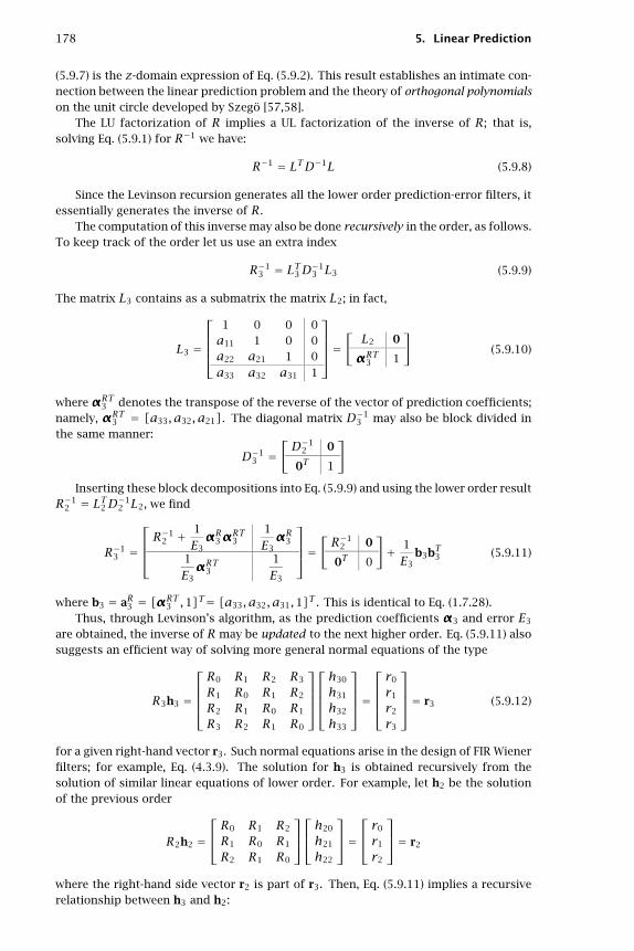
178 5. Linear Prediction
(5.9.7) is the z-domain expression of Eq. (5.9.2). This result establishes an intimate con-nection between the linear prediction problem and the theory of orthogonal polynomialson the unit circle developed by Szego [57,58].
The LU factorization of R implies a UL factorization of the inverse of R; that is,solving Eq. (5.9.1) for R−1 we have:
R−1 = LTD−1L (5.9.8)
Since the Levinson recursion generates all the lower order prediction-error filters, itessentially generates the inverse of R.
The computation of this inverse may also be done recursively in the order, as follows.To keep track of the order let us use an extra index
R−13 = LT3D−1
3 L3 (5.9.9)
The matrix L3 contains as a submatrix the matrix L2; in fact,
L3 =
⎡⎢⎢⎢⎣1 0 0 0a11 1 0 0a22 a21 1 0a33 a32 a31 1
⎤⎥⎥⎥⎦ =[L2 0
αααRT3 1
](5.9.10)
whereαααRT3 denotes the transpose of the reverse of the vector of prediction coefficients;namely, αααRT3 = [a33, a32, a21]. The diagonal matrix D−1
3 may also be block divided inthe same manner:
D−13 =
[D−1
2 0
0T 1
]Inserting these block decompositions into Eq. (5.9.9) and using the lower order result
R−12 = LT2D−1
2 L2, we find
R−13 =
⎡⎢⎢⎣R−12 + 1
E3αααR3ααα
RT3
1
E3αααR3
1
E3αααRT3
1
E3
⎤⎥⎥⎦ =[R−1
2 0
0T 0
]+ 1
E3b3bT3 (5.9.11)
where b3 = aR3 = [αααRT3 ,1]T= [a33, a32, a31,1]T. This is identical to Eq. (1.7.28).Thus, through Levinson’s algorithm, as the prediction coefficients ααα3 and error E3
are obtained, the inverse of Rmay be updated to the next higher order. Eq. (5.9.11) alsosuggests an efficient way of solving more general normal equations of the type
R3h3 =
⎡⎢⎢⎢⎣R0 R1 R2 R3
R1 R0 R1 R2
R2 R1 R0 R1
R3 R2 R1 R0
⎤⎥⎥⎥⎦⎡⎢⎢⎢⎣h30
h31
h32
h33
⎤⎥⎥⎥⎦ =⎡⎢⎢⎢⎣r0
r1
r2
r3
⎤⎥⎥⎥⎦ = r3 (5.9.12)
for a given right-hand vector r3. Such normal equations arise in the design of FIR Wienerfilters; for example, Eq. (4.3.9). The solution for h3 is obtained recursively from thesolution of similar linear equations of lower order. For example, let h2 be the solutionof the previous order
R2h2 =⎡⎢⎣R0 R1 R2
R1 R0 R1
R2 R1 R0
⎤⎥⎦⎡⎢⎣ h20
h21
h22
⎤⎥⎦ =⎡⎢⎣ r0
r1
r2
⎤⎥⎦ = r2
where the right-hand side vector r2 is part of r3. Then, Eq. (5.9.11) implies a recursiverelationship between h3 and h2:

5.9. Orthogonality of Backward Prediction Errors—Cholesky Factorization 179
h3 = R−13 r3 =
⎡⎢⎢⎣R−12 + 1
E3αααR3ααα
RT3
1
E3αααR3
1
E3αααRT3
1
E3
⎤⎥⎥⎦[
r2
r3
]=
⎡⎢⎢⎣ h2 + 1
E3αααR3 (r3 +αααRT3 r2)
1
E3(r3 +αααRT3 r2)
⎤⎥⎥⎦In terms of the reverse prediction-error filter b3 = aR3 = [a33, a32, a31,1]T= [αααRT3 ,1]T,we may write
h3 =[
h2
0
]+ cb3 , where c = 1
E3(r3 +αααRT3 r2)= 1
E3bT3 r3 (5.9.13)
Thus, the recursive updating of the solution h must be done by carrying out the aux-iliary updating of the prediction-error filters. The method requires O(M2) operations,compared to O(M3) if the inverse of R were to be computed directly.
This recursive method of solving general normal equations, developed by Robinsonand Treitel, has been reviewed elsewhere [7,8,59–61]. Some additional insight into theproperties of these recursions can be gained by using the Toeplitz property of R. Thisproperty together with the symmetric nature of R imply that R commutes with thereversing matrix:
J3 =
⎡⎢⎢⎢⎣0 0 0 10 0 1 00 1 0 01 0 0 0
⎤⎥⎥⎥⎦ = J−13 , J3R3J3 = R3 (5.9.14)
Therefore, even though the inverse R−13 is not Toeplitz, it still commutes with this
reversing matrix; that is,J3R−1
3 J3 = R−13 (5.9.15)
The effect of this symmetry property on the block decomposition (5.9.11) may beseen by decomposing J3 also as
J3 =[
0 J2
1 0T
]=
[0T 1J2 0
]
where J2 is the lower order reversing matrix. Combining Eq. (5.9.15) with Eq. (5.9.11),we find
R−13 = J3R−1
3 J3 =[
0T 1J2 0
]⎡⎢⎢⎣R−12 + 1
E3αααR3ααα
RT3
1
E3αααR3
1
E3αααRT3
1
E3
⎤⎥⎥⎦[
0 J2
1 0T
]
or, since R2 commutes with J2, and J2αααR3 =ααα3, we have
R−13 =
⎡⎢⎢⎣1
E3
1
E3αααT3
1
E3ααα3 R−1
2 + 1
E3ααα3αααT3
⎤⎥⎥⎦ =[
0 0T
0 R−12
]+ 1
E3a3aT3 (5.9.16)
which is the same as Eq. (1.7.35). Both ways of expressing R−13 given by Eqs. (5.9.16) and
(5.9.11), are useful. They may be combined as follows: Eq. (5.9.16) gives for the ijthmatrix element:
(R−13 )ij= (R−1
2 +ααα3αααT3E13)i−1,j−1= (R−1
2 )i−1,j−1+α3iα3jE−13
which valid for 1 ≤ i, j ≤ 3. On the other hand, from Eq. (5.9.11) we have

180 5. Linear Prediction
(R−13 )i−1,j−1= (R−1
2 )i−1,j−1+αR3iαR3jE−13
which is valid also for 1 ≤ i, j ≤ 3. Subtracting the two to cancel the common term(R−1
2 )i−1,j−1, we obtain the Goberg-Semencul-Trench-Zohar recursion [62–66]:
(R−13 )ij= (R−1
3 )i−1,j−1+(ααα3αααT3 −αααR3αααRT3 )ijE−13 , 1 ≤ i, j ≤ 3 (5.9.17)
which allows the building-up ofR−13 along each diagonal, provided one knows the “bound-
ary” values to get these recursions started. But these are:
(R−13 )00= E−1
3 , (R−13 )i0= (R−1
3 )0i= a3iE−13 , 1 ≤ i, j ≤ 3 (5.9.18)
Thus, from the prediction-error filter a3 and its reverse, the entire inverse of theautocorrelation matrix may be built up. Computationally, of course, the best procedureis to use Eq. (5.9.8), where L and D are obtained as byproducts of the Levinson recur-sion. The subroutine lev of the appendix starts with the M + 1 autocorrelation lags{R(0),R(1), . . . , R(M)} and generates the required matrices L and D. The main rea-son for the existence of fast algorithms for Toeplitz matrices can be traced to the nestingproperty that the principal submatrices of a Toeplitz matrix are simply the lower orderToeplitz submatrices. Similar fast algorithms have been developed for other types ofstructured matrices, such as Hankel and Vandermonde matrices [67–69].
5.10 Schur Algorithm
The Schur algorithm has its roots in the original work of Schur on the theory of functionsbounded in the unit disk [70,71]. It is an important signal processing tool in a variety ofcontexts, such as linear prediction and signal modeling, fast matrix factorizations, filtersynthesis, inverse scattering, and other applications [71–92].
In linear prediction, Schur’s algorithm is an efficient alternative to Levinson’s algo-rithm and can be used to compute the set of reflection coefficients from the autocor-relation lags and also to compute the conventional LU Cholesky factorization of theautocorrelation matrix. The Schur algorithm is essentially the gapped function recur-sion (5.3.9). It proves convenient to work simultaneously with Eq. (5.3.9) and its reverse.We define the forward and backward gapped functions of order p
g+p (k)= E[e+p (n)yn−k] , g−p (k)= E[e−p (n)yn−k] (5.10.1)
The forward one is identical to that of Eq. (5.3.8). The backward one is the convolu-tion of the backward filter bp = aRp with the autocorrelation function; that is,
g+p (k)=p∑i=0
apiR(k− i) , g−p (k)=p∑i=0
bpiR(k− i) (5.10.2)
where bpi = ap,p−i. In the z-domain, we have
G+p (z)= Ap(z)Syy(z) , G−p (z)= ARp(z)Syy(z) (5.10.3)
Using Syy(z)= Syy(z−1), it follows that
G−p (z)= ARp(z)Syy(z)= z−pAp(z−1)Syy(z−1)= z−pG+p (z−1)
and in the time domain:g−p (k)= g+p (p− k) (5.10.4)

5.10. Schur Algorithm 181
Thus, the backward gapped function is the reflected and delayed version of theforward one. However, the delay is only p units—one less than required to completelyalign the gaps. Therefore, the forward and backward gapped functions have slightlydifferent gaps of length p; namely,
g+p (k) = 0 , for k = 1,2, . . . , p
g−p (k) = 0 , for k = 0,1, . . . , p− 1(5.10.5)
By the definition (5.10. l), the gap conditions of the backward function are equivalentto the orthogonality conditions for the backward predictor; namely, that the estimationerror e−p (n) be orthogonal to the observations {yn−k, k = 0,1, . . . , p − 1} that makeup the estimate of yn−p. Inserting the lattice recursions (5.7.8) into (5.10.1), or usingthe polynomial recursions (5.3.18) into (5.10.3), we obtain the lattice recursions for thegapped functions, known as the Schur recursions
g+p+1(k) = g+p (k)−γp+1g−p (k− 1)
g−p+1(k) = g−p (k− 1)−γp+1g+p (k)(5.10.6)
or, in matrix form [g+p+1(k)g−p+1(k)
]=
[1 −γp+1
−γp+1 1
][g+p (k)g−p (k− 1)
]
They are initialized by g±0 (k)= R(k). The first term of Eq. (5.10.6) is identical to Eq.(5.3.9) and the second term is the reverse of Eq. (5.3.9) obtained by the substitutionk → p + 1 − k. The forward gap condition g+p+1(p + 1)= 0 can be solved for thereflection coefficient
γp+1 =g+p (p+ 1)g−p (p)
(5.10.7)
Note that Eq. (5.10.4) implies g−p (p)= g+p (0)= Ep, and therefore, Eq. (5.10.7) is thesame as Eq. (5.3.11). For an Mth order predictor, we only need to consider the valuesg±p (k), for k = 0,1, . . . ,M. We arrange these values (for the backward function) into thecolumn vector
g−p =
⎡⎢⎢⎢⎢⎢⎣g−p (0)g−p (1)
...g−p (M)
⎤⎥⎥⎥⎥⎥⎦ (5.10.8)
By virtue of the gap conditions (5.10.5), the first p entries, k = 0,1, . . . , p−1, of thisvector are zero. Therefore, we may construct the lower-triangular matrix having the g−p sas columns
G = [g−0 ,g−1 , · · · ,g−M] (5.10.9)
For example, ifM = 3,
G =
⎡⎢⎢⎢⎣g−0 (0) 0 0 0g−0 (1) g−1 (1) 0 0g−0 (2) g−1 (2) g−2 (2) 0g−0 (3) g−1 (3) g−2 (3) g−3 (3)
⎤⎥⎥⎥⎦The first column of G consists simply of theM + 1 autocorrelation lags:
g−0 =
⎡⎢⎢⎢⎢⎢⎣R(0)R(1)
...R(M)
⎤⎥⎥⎥⎥⎥⎦ (5.10.10)

182 5. Linear Prediction
The main diagonal consists of the prediction errors of successive orders, namely,g−p (p)= Ep, for p = 0,1, . . . ,M. Stacking the values of definition (5.10.1) into a vector,we can write compactly,
g−p = E[ep(n)y(n)
](5.10.11)
where y(n)= [yn, yn−1, . . . , yn−M]T is the data vector for anMth order predictor. Thus,the matrix G can be written as in Eq. (1.7.56)
G = E[
y(n)[e−0 (n), e−1 (n), . . . , e−M(n)
]] = E[y(n)e−(n)T
](5.10.12)
where e−(n)= [e−0 (n), e−1 (n), . . . , e−M(n)
]Tis the decorrelated vector of backward pre-
diction errors. Following Eq. (1.7.57), we multiply (5.10.12) from the left by the lowertriangular matrix L, and using the transformation e−(n)= Ly(n) and Eq. (5.9.5), weobtain
LG = LE[y(n)e−(n)T]= E[e−(n)e−(n)T]= DTherefore, G is essentially the inverse of L
G = L−1D (5.10.13)
Using Eq. (5.9.1), we obtain the conventional LU Cholesky factorization of the auto-correlation matrix R in the form
R = L−1DL−T = (GD−1)D(D−1GT)= GD−1GT (5.10.14)
The backward gapped functions are computed by iterating the Schur recursions(5.10.6) for 0 ≤ k ≤ M and 0 ≤ p ≤ M. One computational simplification is that,because of the presence of the gap, the functions g±p (k) need only be computed forp ≤ k ≤ M (actually, g+p (p)= 0 could also be skipped). This gives rise to the Schuralgorithm:
0. Initialize in order by g±0 (k)= R(k), k = 0,1, . . . ,M.
1. At stage p, we have available g±p (k) for p ≤ k ≤M.
2. Compute γp+1 =g+p (p+ 1)g−p (p)
.
3. For p+ 1 ≤ k ≤M, compute
g+p+1(k)= g+p (k)−γp+1g−p (k− 1)
g−p+1(k)= g−p (k− 1)−γp+1g+p (k)
4. Go to stage p+ 1.
5. At the final orderM, set EM = g−M(M).
The subroutine schur (see Appendix B) is an implementation of this algorithm. Theinputs to the routine are the orderM and the lags {R(0),R(1), . . . , R(M)}. The outputsare the parameters {EM,γ1, γ2, . . . , γM}. This routine is a simple alternative to lev. Itmay be used in conjunction with frwlev, bkwlev, and rlev, to pass from one linearprediction parameter set to another. The subroutine schur1 is a small modificationof schur that, in addition to the reflection coefficients, outputs the lower triangularCholesky factor G. The prediction errors can be read off from the main diagonal of G,that is, EP = G(p,p), p = 0,1, . . . ,M.
Example 5.10.1: Sending the five autocorrelation lags, {128,−64,80,−88,89}, of Example 5.3.1through schur1 gives the set of reflection coefficients {γ1, γ2, γ3, γ4} = {−0.5,0.5,−0.5,0.5}, and the matrix G

5.10. Schur Algorithm 183
G =
⎡⎢⎢⎢⎢⎢⎢⎣128 0 0 0 0−64 96 0 0 0
80 −24 72 0 0−88 36 0 54 0
89 −43.5 13.5 13.5 40.5
⎤⎥⎥⎥⎥⎥⎥⎦Recall that the first column should be the autocorrelation lags and the main diagonal shouldconsist of the mean square prediction errors. It is easily verified that GD−1GT = R. ��
The computational bottleneck of the classical Levinson recursion is the computationof the inner product (5.3.12). The Schur algorithm avoids this step by computing γp+1
as the ratio of the two gapped function values (5.10.7). Moreover, at each stage p, thecomputations indicated in step 3 of the algorithm can be done in parallel. Thus, withM parallel processors, the overall computation can be reduced to O(M) operations.VLSI parallel hardware implementations of the Schur algorithm already exist [82,33]. Asformulated above, the Schur algorithm is essentially equivalent to the Le Roux-Gueguenfixed-point algorithm [75]. The possibility of a fixed-point implementation arises fromthe fact that all gapped functions have a fixed dynamic range, bounded by∣∣g±p (k)∣∣ ≤ R(0) (5.10.15)
This is easily seen by applying the Schwarz inequality to definition (5.10.1) and usingEp ≤ R(0)∣∣g±p (k)∣∣2 = ∣∣E[e±p (n)yn−k]∣∣2 ≤ E[e±p (n)2]E[y2
n−k]≤ EpR(0)≤ R(0)2
The Schur algorithm admits a nice filtering interpretation in terms of the lattice struc-ture. By definition, the gapped functions are the convolution of the forward/backwardpth order prediction filters with the autocorrelation sequence R(k). Therefore, g±p (k)will be the outputs from the pth section of the lattice filter, Fig. 5.3, driven by the inputR(k). Moreover, Eq. (5.10.6) states that the (p+1)st reflection coefficient is obtainableas the ratio of the two inputs to the (p+ 1)st lattice section, at time instant p+ 1 (notethat g−p (p)= g−p (p+ 1− 1) is outputted at time p from the pth section and is delayedby one time unit before it is inputted to the (p+1)st section at time p+1.) The correctvalues of the gapped functions g±p (k) are obtained when the input to the lattice filter isthe infinite double-sided sequence R(k). If we send in the finite causal sequence
x(k)= {R(0),R(1), . . . , R(M),0,0, . . . }then, because of the initial and final transient behavior of the filter, the outputs of thepth section will agree with g±p (k) only for p ≤ k ≤M. To see this, let y±p (k) denote thetwo outputs. Because of the causality of the input and filter and the finite length of theinput, the convolutional filtering equation will be
y+p (k)=min{p,k}∑
i=max{0,k−M}api x(k− i)=
min{p,k}∑i=max{0,k−M}
api R(k− i)
This agrees with Eq. (5.10.2) only after time p and before timeM, that is,
y±p (k)= g±p (k) , only for p ≤ k ≤M
The column vector y−p =[y−p (0), y−p (1), . . . , y−p (M)
]T, formed by the first M back-
ward output samples of the pth section, will agree with g−p only for the entries p ≤ k ≤M. Thus, the matrix of backward outputsY− = [y−0 ,y−1 , . . . ,y−M] formed by the columnsy−p will agree with G only in its lower-triangular part. But this is enough to determineG because its upper part is zero.

184 5. Linear Prediction
Example 5.10.2: Send the autocorrelation lags of Example 5.10.1 into the lattice filter of Fig.5.3 (with all its delay registers initialized to zero), arrange the forward/backward outputsfrom the pth section into the column vectors, y±p , and put these columns together to formthe output matrices Y±. The result is,
Y− =
⎡⎢⎢⎢⎢⎢⎢⎣128 64 −64 64 −64−64 96 64 −80 96
80 −24 72 64 −96−88 36 0 54 64
89 −43.5 13.5 13.5 40.5
⎤⎥⎥⎥⎥⎥⎥⎦ , Y+ =
⎡⎢⎢⎢⎢⎢⎢⎣128 128 128 128 128−64 0 −32 −64 −96
80 48 0 32 72−88 −48 −36 0 −32
89 45 27 27 0
⎤⎥⎥⎥⎥⎥⎥⎦The lower-triangular part of Y− agrees with G. The forward/backward outputs y±p can becomputed using, for example, the routine lattice. They can also be computed directly byconvolving the prediction filters with the input. For example, the backward filter of order4 given in Example 5.3.1 is aR4 = [−0.5,0.5,−0.1875,−0.25,1]T . Convolving it with theautocorrelation sequence gives the last column of Y−
[128,−64,80,−88,89]∗[−0.5,0.5,−0.1875,−0.25,1]= [−64,96,−96,64,40.5, . . . ]
Convolving the forward filter a4 with the autocorrelation sequence gives the last columnof the matrix Y+
[128,−64,80,−88,89]∗[1,−0.25,−0.1875,0.5,−0.5]= [128,−96,72,−32,0, . . . ]
Note that we are interested only in the outputs for 0 ≤ k ≤ M = 4. The last 4 outputs (ingeneral, the last p outputs for a pth order filter) of these convolutions were not shown.They correspond to the transient behavior of the filter after the input is turned off. ��
It is also possible to derive a split or immitance-domain version of the Schur algo-rithm that achieves a further 50% reduction in computational complexity [46,47]. Thus,with M parallel processors, the complexity of the Schur algorithm can be reduced toO(M/2) operations. We define a symmetrized or split gapped function in terms of thesymmetric polynomial Fp(z) defined in Eq. (5.6.1)
gp(k)=p∑i=0
fpi R(k− i) , Gp(z)= Fp(z)Syy(z) (5.10.16)
It can be thought of as the output of the filter Fp(z) driven by the autocorrelationsequence. Multiplying both sides of Eq. (5.6.1) by Syy(z) and using the definition (5.10.3),we obtain Gp(z)= G+p−1(z)+z−1G−p−1(z), or, in the time domain
gp(k)= g+p−1(k)+g−p−1(k− 1) (5.10.17)
Similarly, Eq. (5.6.2) gives
(1− γp)gp(k)= g+p (k)+g−p (k) (5.10.18)
It follows from Eqs. (5.10.4) and (5.10.18) or from the symmetry property of Fp(z)that gp(k)= gp(p− k), and in particular, gp(0)= gp(p). The split Levinson algorithmof Section 5.6 requires the computation of the coefficients αp+1 = τp+1/τp. Settingk = 0 in the definition (5.10.16) and using the reflection symmetry R(i)= R(−i), werecognize that the inner product of Eq. (5.6.6) is τp = gp(0)= gp(p). Therefore, thecoefficient αp+1 can be written as the ratio of the two gapped function values
αp+1 = gp+1(p+ 1)gp(p)
(5.10.19)

5.10. Schur Algorithm 185
Because the forward and backward gapped functions have overlapping gaps, it fol-lows that gp(k) will have gap gp(k)= 0, for k = 1,2, . . . , p− 1. Therefore, for an Mthorder predictor, we only need to know the values of gp(k) for p ≤ k ≤ M. Thesecan be computed by the following three-term recurrence, obtained by multiplying therecurrence (5.6.4) by Syy(z)
gp+2(k)= gp+1(k)+gp+1(k− 1)−αp+1gp(k− 1) (5.10.20)
Using F0(z)= 2 and F1(z)= 1 + z−1, it follows from the definition that g0(k)=2R(k) and g1(k)= R(k)+R(k−1). To initialize τ0 correctly, however, we must chooseg0(0)= R(0), so that τ0 = g0(0)= R(0). Thus, we are led to the following split Schuralgorithm:
0. Initialize by g0(k)= 2R(k), g1(k)= R(k)+R(k − 1), for k = 1,2, . . . ,M, andg0(0)= R(0), γ0 = 0.
1. At stage p, we have available γp, gp(k) for p ≤ k ≤ M, and gp+1(k) for p+ 1 ≤k ≤M.
2. Compute αp+1 from Eq. (5.10.19) and solve for γp+1 = −1+αp+1/(1− γp).3. For p+ 2 ≤ k ≤M, compute gp+2(k) using Eq. (5.10.20)
4. Go to stage p+ 1.
Recalling that Ep = τp(1 − γp), we may set at the final order EM = τM(1 − γM)=gM(M)(1 − γM). Step 3 of the algorithm requires only one multiplication for each k,whereas step 3 of the ordinary Schur algorithm requires two. This reduces the com-putational complexity by 50%. The subroutine schur2 (see Appendix B) is an imple-mentation of this algorithm. The inputs to the routine are the order M and the lags{R(0),R(1), . . . , R(M)}. The outputs are the parameters {EM,γ1, γ2, . . . , γM}. Theroutine can be modified easily to include the computation of the backward gapped func-tions g−p (k), which are the columns of the Cholesky matrix G. This can be done by therecursion
g−p (k)= g−p (k− 1)+(1− γp)gp(k)−gp+1(k) (5.10.21)
where p + 1 ≤ k ≤ M, with starting value g−p (p)= Ep = gp(p)(1 − γp). This recur-sion will generate the lower-triangular part of G. Equation (5.10.21) follows by writingEq. (5.10.17) for order (p + 1) and subtracting it from Eq. (5.10.18). Note, also, thatEq. (5.10.17) and the bound (5.10.15) imply the bound |gp(k)| ≤ 2R(0), which allows afixed-point implementation.
We finish this section by discussing the connection of the Schur algorithm to Schur’soriginal work. It follows from Eq. (5.10.3) that the ratio of the two gapped functionsG±p (z) is an all-pass stable transfer function, otherwise known as a lossless bounded realfunction [56]:
Sp(z)=G−p (z)G+p (z)
= ARp(z)Ap(z)
= app + ap,p−1z−1 + · · · + z−p1+ ap1z−1 + · · · + appz−p (5.10.22)
The all-pass property follows from the fact that the reverse polynomial AR(z) hasthe same magnitude response asAp(z). The stability property follows from the minimum-phase property of the polynomials Ap(z), which in turn is equivalent to all reflectioncoefficients having magnitude less than one. Such functions satisfy the boundednessproperty ∣∣Sp(z)∣∣ ≤ 1 , for |z| ≥ 1 (5.10.23)
with equality attained on the unit circle. Taking the limit z → ∞, it follows fromEq. (5.10.22) that the reflection coefficient γp is obtainable from Sp(z) by
Sp(∞)= app = −γp (5.10.24)

186 5. Linear Prediction
Using the backward Levinson recursion (5.3.23), we obtain a new all-pass function
Sp−1(z)=G−p−1(z)G+p−1(z)
= ARp−1(z)Ap−1(z)
= z(γpAp +ARp)
Ap + γpARpor, dividing numerator and denominator by Ap(z)
Sp−1(z)= z Sp(z)+γp1+ γpSp(z) (5.10.25)
This is Schur’s original recursion [70]. Applying this recursion repeatedly from someinitial value p =M down to p = 0, with S0(z)= 1, will give rise to the set of reflection orSchur coefficients {γ1, γ2, . . . , γM}. The starting all-pass function SM(z) will be stableif and only if all reflection coefficients have magnitude less than one. We note finallythat there is an intimate connection between the Schur algorithm and inverse scatteringproblems [76, 79, 80, 86, 87, 90–92, 138]. In Section 5.13, we will see that the lattice re-cursions (5.10.6) describe the forward and backward moving waves incident on a layeredstructure. The Schur function Sp(z) will correspond to the overall reflection responseof the structure, and the recursion (5.10.25) will describe the successive removal of thelayers. The coefficients γp will represent the elementary reflection coefficients at thelayer interfaces. This justifies the term reflection coefficients for the γs.
5.11 Lattice Realizations of FIR Wiener Filters
In this section, we combine the results of Sections 4.3 and 5.9 to derive alternativerealizations of Wiener filters that are based on the Gram-Schmidt lattice structures.Consider the FIR Wiener filtering problem of estimating a desired signal xn, on the basisof the related signal yn, using anMth order filter. The I/O equation of the optimal filteris given by Eq. (4.3.8). The vector of optimal weights is determined by solving the set ofnormal equations, given by Eq. (4.3.9). The discussion of the previous section suggeststhat Eq. (4.3.9) can be solved efficiently using the Levinson recursion. Defining the datavector
y(n)=
⎡⎢⎢⎢⎢⎢⎣ynyn−1
...yn−M
⎤⎥⎥⎥⎥⎥⎦ (5.11.1)
we rewrite Eq. (4.3.9) in the compact matrix form
Ryyh = rxy (5.11.2)
where Ryy is the (M+1)×(M+1) autocorrelation matrix of y(n), and rxy, the (M+1)-vector of cross-correlations between xn, and y(n), namely,
Ryy = E[y(n)y(n)T
], rxy = E[xny(n)]=
⎡⎢⎢⎢⎢⎢⎣Rxy(0)Rxy(1)
...Rxy(M)
⎤⎥⎥⎥⎥⎥⎦ (5.11.3)
and h is the (M + 1)-vector of optimal weights
h =
⎡⎢⎢⎢⎢⎢⎣h0
h1
...hM
⎤⎥⎥⎥⎥⎥⎦ (5.11.4)

5.11. Lattice Realizations of FIR Wiener Filters 187
The I/O equation of the filter, Eq. (5.9.4), is
xn = hTy(n)= h0yn + h1yn−1 + · · · + hMyn−M (5.11.5)
Next, consider the Gram-Schmidt transformation of Eq. (5.9.4) from the data vectory(n) to the decorrelated vector e−(n):
e−(n)= Ly(n) or,
⎡⎢⎢⎢⎢⎢⎣e−0 (n)e−1 (n)
...e−M(n)
⎤⎥⎥⎥⎥⎥⎦ = L⎡⎢⎢⎢⎢⎢⎣ynyn−1
...yn−M
⎤⎥⎥⎥⎥⎥⎦ (5.11.6)
Inserting Eq. (5.11.6) into Eq. (5.11.5), we find
xn = hTL−1e−(n)
Defining the (M + 1)-vectorg = L−Th (5.11.7)
we obtain the alternative I/O equation for the Wiener filter:
xn = gTe−(n)=M∑p=0
gpe−p (n)= g0e−0 (n)+g1e−1 (n)+· · · + gMe−M(n) (5.11.8)
This is easily recognized as the projection of xn onto the subspace spanned by{e−0 (n), e−1 (n), . . . , e−M(n)
}, which is the same as that spanned by the data vector {yn,
yn−1, . . . , yn−M}. Indeed, it follows from Eqs. (5.11.7) and (5.11.2) that
gT = hTL−1 = E[xny(n)T]E[y(n)y(n)T]−1L−1
= E[xne−(n)T]L−T(L−1E[e−(n)e−(n)T]L−T
)−1L−1
= E[xne−(n)T]E[e−(n)e−(n)T]−1
= [E[xne−0 (n)]/E0, E[xne−1 (n)]/E1, . . . , E[xne−M(n)]/EM
]so that the estimate of xn can be expressed as
xn = E[xne−(n)T]E[e−(n)e−(n)T]−1e−(n)= E[xny(n)T]E[y(n)y(n)T]−1y(n)
The key to the lattice realization of the optimal filtering equation (5.11.8) is theobservation that the analysis lattice filter of Fig. 5.3 for the process yn, provides, in itssuccessive lattice stages, the signals e−p (n)which are required in the sum (5.11.8). Thus,if the weight vector g is known, an alternative realization of the optimal filter will be asshown in Fig. 5.5. By comparison, the direct form realization using Eq. (5.11.5) operatesdirectly on the vector y(n), which, at each time instant n, is available at the tap registersof the filter. This is depicted in Fig. 5.6.
Both types of realizations can be formulated adaptively, without requiring priorknowledge of the filter coefficients or the correlation matrices Ryy and rxy. We willdiscuss adaptive implementations in Chapter 7. If Ryy and rxy are known, or can be es-timated, then the design procedure for both the lattice and the direct form realizationsis implemented by the following three steps:
1. Using Levinson’s algorithm, implemented by the subroutine lev, perform the LUCholesky factorization of Ryy, to determine the matrices L and D.

188 5. Linear Prediction
Fig. 5.5 Lattice realization of FIR Wiener filter.
Fig. 5.6 Direct-form realization of FIR Wiener filter.
2. The vector of weights g can be computed in terms of the known quantities L,D, rxyas follows:
g = L−Th = L−TR−1yy rxy = L−T
(LTD−1L
)rxy = D−1Lrxy
3. The vector h can be recovered from g by h = LTg.
The subroutine firw (see Appendix B) is an implementation of this design procedure.The inputs to the subroutine are the orderM and the correlation lags
{Ryy(0),Ryy(1),

5.11. Lattice Realizations of FIR Wiener Filters 189
. . . , Ryy(M)}
and{Rxy(0),Rxy(1), . . . , Rxy(M)
}. The outputs are the quantities L,D,g,
and h. The estimate (5.11.8) may also be written recursively in the order of the filter. Ifwe denote,
xp(n)=p∑i=0
gie−i (n) (5.11.9)
we obtain the recursion
xp(n)= xp−1(n)+gpe−p (n) , p = 0,1, . . . ,M (5.11.10)
initialized as x−1(n)= 0. The quantity xp(n) is the projection of xn on the subspacespanned by
{e−0 (n), e−1 (n), . . . , e−p (n)
}, which by virtue of the lower-triangular nature
of the matrix L is the same space as that spanned by {yn, yn−1, . . . , yn−p}. Thus, xp(n)represents the optimal estimate of xn based on a pth order filter. Similarly, xp−1(n)represents the optimal estimate of xn based on the (p− 1)th order filter; that is, basedon the past p− 1 samples {yn, yn−1, . . . , yn−p+1}. These two subspaces differ by yn−p.
The term e−p (n) is by construction the best postdiction error of estimating yn−p fromthe samples {yn, yn−1, . . . , yn−p+1}; that is, e−p (n) is the orthogonal complement of yn−pprojected on that subspace. Therefore, the term gpe−p (n) in Eq. (5.11.10) represents theimprovement in the estimate of xn that results by taking into account the additionalpast value yn−p; it represents that part of xn that cannot be estimated in terms of thesubspace {yn, yn−1, . . . , yn−p+1}. The estimate xp(n) of xn is better than xp−1(n) in thesense that it produces a smaller mean-squared estimation error. To see this, define theestimation errors in the two cases
ep(n)= xn − xp(n) , ep−1(n)= xn − xp−1(n)
Using the recursion (5.11.10), we find
ep(n)= ep−1(n)−gpe−p (n) (5.11.11)
Using gp = E[xne−p (n)]/Ep, we find for Ep = E[ep(n)2]
Ep = E[x2n]−
p∑i=0
giE[xne−i (n)]= Ep−1 − gpE[xne−p (n)]
= Ep−1 −(E[xne−p (n)]
)2/Ep = Ep−1 − g2pEp
Thus, Ep is smaller than Ep−1. This result shows explicitly how the estimate is con-stantly improved as the length of the filter is increased. The nice feature of the latticerealization is that the filter length can be increased simply by adding more lattice sec-tions without having to recompute the weights gp of the previous sections. A realizationequivalent to Fig. 5.5, but which shows explicitly the recursive construction (5.11.10) ofthe estimate of xn and of the estimation error (5.11.11), is shown in Fig. 5.7.
The subroutine lwf (see Appendix B) is an implementation of the lattice Wiener fil-ter of Fig. 5.7. The routine dwf implements the direct-form Wiener filter of Fig. 5.6.Each call to these routines transforms a pair of input samples {x, y} into the pair ofoutput samples {x, e} and updates the internal state of the filter. Successive calls overn = 0,1,2, . . . , will transform the input sequences {xn, yn} into the output sequences{xn, en}. In both realizations, the internal state of the filter is taken to be the vector ofsamples stored in the delays of the filter; that is, wp(n)= e−p−1(n− 1), p = 1,2, . . . ,Mfor the lattice case, and wp(n)= yn−p, p = 1,2, . . . ,M for the direct-form case. Byallowing the filter coefficients to change between calls, these routines can be used inadaptive implementations.

190 5. Linear Prediction
Fig. 5.7 Lattice realization of FIR Wiener filter.
Next, we present a Wiener filter design example for a noise canceling application.The primary and secondary signals x(n) and y(n) are of the form
x(n)= s(n)+v1(n) , y(n)= v2(n)
where s(n) is a desired signal corrupted by noise v1(n). The signal v2(n) is correlatedwith v1(n) but not with s(n), and provides a reference noise signal. The noise canceleris to be implemented as a Wiener filter of order M, realized either in the direct or thelattice form. It is shown below:
Its basic operation is that of a correlation canceler; that is, the optimally designedfilter H(z) will transform the reference noise v2(n) into the best replica of v1(n), andthen proceed to cancel it from the output, leaving a clean signal s(n). For the purposeof the simulation, we took s(n) to be a simple sinusoid
s(n)= sin(ω0n) , ω0 = 0.075π [rads/sample]
and v1(n) and v2(n) were generated by the difference equations
v1(n) = −0.5v1(n− 1)+v(n)v2(n) = 0.8v2(n− 1)+v(n)
driven by a common, zero-mean, unit-variance, uncorrelated sequence v(n). The dif-ference equations establish a correlation between the two noise components v1 and v2,which is exploited by the canceler to effect the noise cancellation.
Figs. 5.8 and 5.9 show 100 samples of the signals x(n), s(n), and y(n) generatedby a particular realization of v(n). For M = 4 and M = 6, the sample autocorrelationand cross-correlation lags, Ryy(k), Rxy(k), k = 0,1, . . . ,M, were computed and sentthrough the routine firw to get the filter weights g and h.
The reference signal yn was filtered through H(z) to get the estimate xn—whichis really an estimate of v1(n)—and the estimation error e(n)= x(n)−x(n), which isreally an estimate of s(n). This estimate of s(n) is shown in Figs. (5.10) and 5.11, for

5.11. Lattice Realizations of FIR Wiener Filters 191
0 20 40 60 80 100−4
−3
−2
−1
0
1
2
3
4
time samples, n
primary signal x(n)
x(n) = s(n) + v1(n) s(n) = sin(ω0n)
Fig. 5.8 Noise corrupted sinusoid.
0 20 40 60 80 100−4
−3
−2
−1
0
1
2
3
4
time samples, n
secondary signal y(n)
y(n) = v2(n)
Fig. 5.9 Reference noise.
the casesM = 4 andM = 6, respectively. The improvement afforded by a higher orderfilter is evident. For the particular realization of x(n) and y(n) that we used, the samplecorrelations Ryy(k), Rxy(k), k = 0,1, . . . ,M, were:
Ryy = [2.5116, 1.8909, 1.2914, 0.6509, 0.3696, 0.2412, 0.1363]
Rxy = [0.7791, −0.3813, 0.0880, −0.3582, 0.0902, −0.0684, 0.0046]
and the resulting vector of lattice weights gp, p = 0,1, . . . ,M, reflection coefficients γp,p = 1,2, . . . ,M, and direct-form weights hm,m = 0,1, . . . ,M were forM = 6,
g = [0.3102, −0.8894, 0.4706, −0.2534, 0.1571, −0.0826, 0.0398]
γγγ = [0.7528, −0.1214, −0.1957, 0.1444, 0.0354, −0.0937]
h = [0.9713, −1.2213, 0.6418, −0.3691, 0.2245, −0.1163, 0.0398]
To get the g and γγγ of the case M = 4, simply ignore the last two entries in the above.The corresponding h is in this case:
h = [0.9646, −1.2262, 0.6726, −0.3868, 0.1571]
Using the results of Problems 5.25 and 5.26, we may compute the theoretical filterweights for this example, and note that they compare fairly well with the estimated ones

192 5. Linear Prediction
0 20 40 60 80 100−4
−3
−2
−1
0
1
2
3
4
time samples, n
recovered signal e(n)
e(n) s(n)
Fig. 5.10 Output of noise canceler (M = 4).
0 20 40 60 80 100−4
−3
−2
−1
0
1
2
3
4
time samples, n
recovered signal e(n)
e(n) s(n)
Fig. 5.11 Output of noise canceler (M = 6).
that were based on the length-100 data blocks. ForM = 6, we have:
g = [0.2571, −0.9286, 0.4643, −0.2321, 0.1161, −0.0580, 0.0290]
γγγ = [0.8, 0, 0, 0, 0, 0]
h = [1, −1.3, 0.65, −0.325, 0.1625, −0.0812, 0.0290]
As we discussed in Section 1.7, the lattice realizations based on the backward orthog-onal basis have three major advantages over the direct-form realizations: (a) the filterprocesses non-redundant information only, and hence adaptive implementations wouldadapt faster; (b) the design of the optimal filter weights g does not require any matrixinversion; and (c) the lower-order portions of g are already optimal. Moreover, it appearsthat adaptive versions of the lattice realizations have better numerical properties thanthe direct-form versions. In array processing problems, because the data vector y(n)does not have the tapped-delay line form (5.11.1), the Gram-Schmidt orthogonalizationcannot be done by a simple a lattice filter. It requires a more complicated structure thatbasically amounts to carrying out the lower-triangular linear transformation (5.11.6).The benefits, however, are the same. We discuss adaptive versions of Gram-Schmidtpreprocessors for arrays in Chapter 7.

5.12. Autocorrelation, Covariance, and Burg’s Methods 193
5.12 Autocorrelation, Covariance, and Burg’s Methods
As mentioned in Section 5.3, the finite order linear prediction problem may be thoughtof as an approximation to the infinite order prediction problem. For large enough orderp of the predictor, the prediction-error filter Ap(z) may be considered to be an ade-quate approximation to the whitening filter A(z) of the process yn. In this case, theprediction-error sequence e+p (n) is approximately white, and the inverse synthesis filter1/Ap(z) is an approximation to the signal model B(z) of yn. Thus, we have obtainedan approximate solution to the signal modeling problem depicted below:
The variance of e+p (n) is Ep. Depending on the realization one uses, the model pa-rameters are either the set {ap1, ap2, . . . , app;Ep}, or, {γ1, γ2, . . . , γp;Ep}. Because thesecan be determined by solving a simple linear system of equations—that is, the normalequations (5.3.7)—this approach to the modeling problem has become widespread.
In this section, we present three widely used methods of extracting the model pa-rameters from a given block of measured signal values yn [3,6,10,11,93–103]. Thesemethods are:
1. The autocorrelation, or Yule-Walker, method2. The covariance method.3. Burg’s method.
We have already discussed the Yule-Walker method, which consists simply of replac-ing the theoretical autocorrelations Ryy(k) with the corresponding sample autocorre-lations Ryy(k) computed from the given frame of data. This method, like the othertwo, can be justified on the basis of an appropriate least-squares minimization criterionobtained by replacing the ensemble averages E[e+p (n)2] by appropriate time averages.
The theoretical minimization criteria for the optimal forward and backward predic-tors are
E[e+p (n)2]= min , E[e−p (n)2]= min (5.12.1)
where e+p (n) and e−p (n) are the result of filtering yn through the prediction-error fil-ter a = [1, ap1, . . . , app]T and its reverse aR = [app, ap,p−1, . . . , ap1,1]T, respectively;namely,
e+p (n) = yn + ap1yn−1 + ap2yn−2 + · · · + appyn−pe−p (n) = yn−p + ap1yn−p+1 + ap2yn−p+2 + · · · + appyn
(5.12.2)
Note that in both cases the mean-square value of e±p (n) can be expressed in termsof the (p+ 1)×(p+ 1) autocorrelation matrix
R(i, j)= R(i− j)= E[yn+i−jyn]= E[yn−jyn−i] , 0 ≤ i, j ≤ pas follows
E[e+p (n)2]= E[e−p (n)2]= aTRa (5.12.3)
Consider a frame of length N of measured values of yn
y0, y1, . . . , yN−1
1. The Yule-Walker, or autocorrelation, method replaces the ensemble average (5.12.1)by the least-squares time-average criterion
E =N+p−1∑n=0
e+p (n)2= min (5.12.4)

194 5. Linear Prediction
where e+p (n) is obtained by convolving the length-(p + 1) prediction-error filter a =[1, ap1, . . . , app]T with the length-N data sequence yn. The length of the sequencee+p (n) is, therefore, N + (p + 1)−1 = N + p, which justifies the upper-limit in thesummation of Eq. (5.12.4). This convolution operation is equivalent to assuming thatthe block of data yn has been extended both to the left and to the right by padding itwith zeros and running the filter over this extended sequence. The last p output samplese+p (n), N ≤ n ≤ N + p − 1, correspond to running the filter off the ends of the datasequence to the right. These terms arise because the prediction-error filter has memoryof p samples. This is depicted below:
Inserting Eq. (5.12.2) into (5.12.4), it is easily shown that E can be expressed in theequivalent form
E =N+p−1∑n=0
e+p (n)2=p∑i,j=0
aiR(i− j)aj = aTRa (5.12.5)
where R(k) denotes the sample autocorrelation of the length-N data sequence yn:
R(k)= R(−k)=N−1−k∑n=0
yn+kyn , 0 ≤ k ≤ N − 1
where the usual normalization factor 1/N has been ignored. This equation is identicalto Eq. (5.12.3) with R replaced by R. Thus, the minimization of the time-average index(5.12.5) with respect to the prediction coefficients will lead exactly to the same set ofnormal equations (5.3.7) with R replaced by R. The positive definiteness of the sampleautocorrelation matrix also guarantees that the resulting prediction-error filter will beminimum phase, and thus also that all reflection coefficients will have magnitude lessthan one.
2. The covariance method replaces Eq. (5.12.1) by the time average
E =N−1∑n=pe+p (n)2= min (5.12.6)
where the summation in n is such that the filter does not run off the ends of the datablock, as shown below:
To explain the method and to see its potential problems with stability, consider asimple example of a length-three sequence and a first-order predictor:
E =2∑n=1
e+1 (n)2= e+1 (1)2+e+1 (2)2= (y1 + a11y0)2+(y2 + a11y1)2

5.12. Autocorrelation, Covariance, and Burg’s Methods 195
Differentiating with respect to a11 and setting the derivative to zero gives
(y1 + a11y0)y0 + (y2 + a11y1)y1 = 0
a11 = −y1y0 + y2y1
y20 + y2
1
Note that the denominator does not depend on the variable y2 and therefore it ispossible, if y2 is large enough, for a11 to have magnitude greater than one, makingthe prediction-error filter nonminimal phase. Although this potential stability problemexists, this method has been used with good success in speech processing, with few,if any, such stability problems. The autocorrelation method is sometimes preferred inspeech processing because the resulting normal equations have a Toeplitz structure andtheir solution can be obtained efficiently using Levinson’s algorithm. However, similarways of solving the covariance equations have been developed recently that are just asefficient [98].
3. Although the autocorrelation method is implemented efficiently, and the resultingprediction-error filter is guaranteed to be minimum phase, it suffers from the effect ofwindowing the data sequence yn, by padding it with zeros to the left and to the right.This reduces the accuracy of the method somewhat, especially when the data record Nis short. In this case, the effect of windowing is felt more strongly. The proper wayto extend the sequence yn, if it must be extended, is a way compatible with the signalmodel generating this sequence. Since we are trying to determine this model, the fairestway of proceeding is to try to use the available data block in a way which is maximallynoncommittal as to what the sequence is like beyond the ends of the block.
Burg’s method, also known as the maximum entropy method (MEM), arose from thedesire on the one hand not to run off the ends of the data, and, on the other, to alwaysresult in a minimum-phase filter. Burg’s minimization criterion is to minimize the sum-squared of both the forward and the backward prediction errors:
E =N−1∑n=p
[e+p (n)2+e−p (n)2] = min (5.12.7)
where the summation range is the same as in the covariance method, but with both theforward and the reversed filters running over the data, as shown:
If the minimization is performed with respect to the coefficients api, it is still possi-ble for the resulting prediction-error filter not to be minimum phase. Instead, Burg sug-gests an iterative procedure: Suppose that the prediction-error filter [1, ap−1,1, ap−1,2,. . . , ap−1,p−1] of order (p − 1) has already been determined. Then, to determine theprediction-error filter of order p, one needs to know the reflection coefficient γp and toapply the Levinson recursion:⎡⎢⎢⎢⎢⎢⎢⎢⎢⎢⎣
1ap1
ap2
...ap,p−1
app
⎤⎥⎥⎥⎥⎥⎥⎥⎥⎥⎦=
⎡⎢⎢⎢⎢⎢⎢⎢⎢⎢⎣
1ap−1,1ap−1,2
...ap−1,p−1
0
⎤⎥⎥⎥⎥⎥⎥⎥⎥⎥⎦− γp
⎡⎢⎢⎢⎢⎢⎢⎢⎢⎢⎣
0ap−1,p−1
ap−1,p−2
...ap−1,11
⎤⎥⎥⎥⎥⎥⎥⎥⎥⎥⎦(5.12.8)

196 5. Linear Prediction
To guarantee the minimum-phase property, the reflection coefficient γp must havemagnitude less than one. The best choice for γp is that which minimizes the perfor-mance index (5.12.7). Differentiating with respect to γp and setting the derivative tozero we find
∂E∂γp
= 2N−1∑n=p
[e+p (n)
∂e+p (n)∂γp
+ e−p (n)∂e−p (n)∂γp
]= 0
Using the lattice relationships
e+p (n) = e+p−1(n)−γpe−p−1(n− 1)
e−p (n) = e−p−1(n− 1)−γpe+p−1(n)(5.12.9)
both valid for p ≤ n ≤ N − 1 if the filter is not to run off the ends of the data, we findthe condition
N−1∑n=p
[e+p (n)e
−p−1(n− 1)+e−p (n)e+p−1(n)
] = 0 , or,
N−1∑n=p
[(e+p−1(n)−γpe−p−1(n− 1)
)e−p−1(n− 1)+(
e−p−1(n− 1)−γpe+p−1(n))e+p−1(n)
] = 0
which can be solved for γp to give
γp =2N−1∑n=pe+p−1(n)e
−p−1(n− 1)
N−1∑n=p
[e+p−1(n)2+e−p−1(n− 1)2] (5.12.10)
This expression for γp is of the form
γp = 2a · b
|a|2 + |b|2where a and b are vectors. Using the Schwarz inequality, it is easily verified that γp hasmagnitude less than one. Equations (5.12.8) through (5.12.10) define Burg’s method.The computational steps are summarized below:
0. Initialize in order as follows:
e+0 (n)= e−0 (n)= yn , for 0 ≤ n ≤ N − 1 , and A0(z)= 1, E0 = 1
N
N−1∑n=0
y2n
1. At stage (p− 1), we have available the quantities:
Ap−1(z), Ep−1, and e±p−1(n), for p− 1 ≤ n ≤ N − 1
2. Using Eq. (5.12.10), compute the reflection coefficient γp.
3. Using (5.12.8), compute Ap(z).4. Using (5.12.9), compute e±p (n), for p ≤ n ≤ N − 1.
5. Update the mean-square error by Ep = (1− γ2p)Ep−1.
6. Go to stage p.
The subroutine burg (see Appendix B) is an implementation of this method. The in-puts to the subroutine are the vector of data samples {y0, y1, . . . , yN−1} and the desiredfinal order M of the predictor. The outputs are all the prediction-error filters of orderup to M, arranged as usual into the lower triangular matrix L, and the correspondingmean-square prediction errors {E0, E1, . . . , EM}.

5.12. Autocorrelation, Covariance, and Burg’s Methods 197
Example 5.12.1: The length-six block of data
yn = [4.684, 7.247, 8.423, 8.650, 8.640, 8.392]
forn = 0,1,2,3,4,5, is known to have been generated by sending zero-mean, unit-variance,white-noise εn through the difference equation
yn − 1.70yn−1 + 0.72yn−2 = εn
Thus, the theoretical prediction-error filter and mean-square error areA2(z)= 1−1.70z−1+0.72z−2 and E2 = 1. Using Burg’s method, extract the model parameters for a second-ordermodel. The reader is urged to go through the algorithm by hand. Sending the above sixyn samples through the routine burg, we find the first- and second-order prediction-errorfilters and the corresponding errors:
A1(z) = 1− 0.987z−1 , E1 = 1.529
A2(z) = 1− 1.757z−1 + 0.779z−2 , E2 = 0.60
We note that the theoretical first-order filter obtained from A2(z)= 1−1.70z−1+0.72z−2
via the backward Levinson recursion is A1(z)= 1− 0.9884z−1. ��
The resulting set of LPC model parameters, from any of the above analysis methods,can be used in a number of ways as suggested in Section 1.11. One of the most successfulapplications has been to the analysis and synthesis of speech [6,104–112]. Each frameof speech, of duration of the order of 20 msec, is subjected to the Yule-Walker analysismethod to extract the corresponding set of model parameters. The order M of thepredictor is typically 10–15. Pitch and voiced/unvoiced information are also extracted.The resulting set of parameters represents that speech segment.
To synthesize the segment, the set of model parameters are recalled from memoryand used in the synthesizer to drive the synthesis filter. The latter is commonly realizedas a lattice filter. Lattice realizations are preferred because they are much better well-behaved under quantization of their coefficients (i.e., the reflection coefficients) thanthe direct-form realizations [6,108,109]. A typical speech analysis and synthesis systemis shown in Fig. 5.12.
Fig. 5.12 LPC analysis and synthesis of speech.
Linear predictive modeling techniques have also been applied to EEG signal process-ing in order to model EEG spectra, to classify EEGs automatically, to detect EEG transientsthat might have diagnostic significance, and to predict the onset of epileptic seizures[113–120].
LPC methods have been applied successfully to signal classification problems such asspeech recognition [107,121-126] or the automatic classification of EEGs [117]. Distancemeasures between two sets of model parameters extracted from two signal frames can

198 5. Linear Prediction
be used as measures of similarity between the frames. Itakura’s LPC distance measurecan be introduced as follows: Consider two autoregressive signal sequences, the testsequence yT(n) to be compared against the reference sequence yR(n). Let AT(z) andAR(z) be the two whitening filters, both of orderM. The two signal models are
Now, suppose the sequence to be tested, yT(n), is filtered through the whiteningfilter of the reference signal
resulting in the output signal eT(n). The mean output power is easily expressed as
E[eT(n)2] = a†RRTaR =∫ π−πSeTeT(ω)
dω2π
=∫ π−π
∣∣AR(ω)∣∣2SyTyT(ω)dω2π
=∫ π−π
∣∣AR(ω)∣∣2 σ2εT∣∣AT(ω)∣∣2
dω2π
where RT is the autocorrelation matrix of yT(n). On the other hand, if yT(n) is filteredthrough its own whitening filter, it will produce εT(n). Thus, in this case
σ2εT = E[εT(n)2]= a†TRTaT
It follows thatE[eT(n)2]E[εT(n)2]
= a†RRTaR
a†TRTaT=
∫ π−π
∣∣AR(ω)∣∣2∣∣AT(ω)∣∣2
dω2π
(5.12.11)
The log of this quantity is Itakura’s LPC distance measure
d(aT, aR)= log
(E[eT(n)2]E[εT(n)2]
)= log
(a†RRTaR
a†TRTaT
)= log
[∫ π−π
∣∣AR(ω)∣∣2∣∣AT(ω)∣∣2
dω2π
]
In practice, the quantities aT, RT, and aR are extracted from a frame of yT(n) and aframe of yR(n). If the model parameters are equal, the distance is zero. This distancemeasure effectively provides a comparison between the two spectra of the processesyT and yR, but instead of comparing them directly, a prewhitening of yT(n) is carriedout by sending it through the whitening filter of the other signal. If the two spectraare close, the filtered signal eT(n) will be close to white—that is, with a spectrum closeto being flat; a measure of this flatness is precisely the above integrated spectrum ofEq. (5.12.11).
5.13 Dynamic Predictive Deconvolution—Waves in Layered Me-
dia
The analysis and synthesis lattice filters, implemented via the Levinson recursion, wereobtained within the context of linear prediction. Here, we would like to point out the re-markable fact that the same analysis and synthesis lattice structures also occur naturallyin the problem of wave propagation in layered media [6,7,9,59,61,95,104,127–144]. Thisis perhaps the reason behind the great success of linear prediction methods in speechand seismic signal processing. In fact, historically many linear prediction techniqueswere originally developed within the context of these two application areas.

5.13. Dynamic Predictive Deconvolution—Waves in Layered Media 199
In speech, the vocal tract is modeled as an acoustic tube of varying cross-sectionalarea. It can be approximated by the piece-wise constant area approximation shownbelow:
The acoustic impedance of a sound wave varies inversely with the tube area
Z = ρcA
where ρ, c,A are the air density, speed of sound, and tube area, respectively. Therefore,as the sound wave propagates from the glottis to the lips, it will suffer reflections everytime it encounters an interface; that is, every time it enters a tube segment of differ-ent diameter. Multiple reflections will be set up within each segment and the tube willreverberate in a complicated manner depending on the number of segments and thediameter of each segment. By measuring the speech wave that eventually comes out ofthe lips, it is possible to remove, or deconvolve, the reverberatory effects of the tubeand, in the process, extract the tube parameters, such as the areas of the segments or,equivalently, the reflection coefficients at the interfaces. During speech, the configu-ration of the vocal tract tube changes continuously. But being a mechanical system, itdoes so fairly slowly, and for short periods of time (of the order of 20–30 msec) it maybe assumed to maintain a fixed configuration. From each such short segment of speech,a set of configuration parameters (e.g., reflection coefficients) may be extracted. Thisset may be used to synthesize the speech segment.
The seismic problem is somewhat different. Here it is not the transmitted wave thatis experimentally accessible, but rather the overall reflected wave:
An impulsive input to the earth, such as a dynamite explosion near the surface,will set up seismic elastic waves propagating downwards. As the various earth layersare encountered, reflections will take place. Eventually each layer will be reverberatingand an overall reflected wave will be measured at the surface. On the basis of thisreflected wave, the layered structure (i.e., reflection coefficients, impedances, etc.) mustbe extracted by deconvolution techniques. These are essentially identical to the linearprediction methods.
In addition to geophysical and speech applications, this wave problem and the as-sociated inverse problem of extracting the structure of the medium from the observed(reflected or transmitted) response have a number of other applications. Examples in-clude the probing of dielectric materials by electromagnetic waves, the study of theoptical properties of thin films, the probing of tissues by ultrasound, and the designof broadband terminations of transmission lines. The mathematical analysis of suchwave propagation problems has been done more or less independently in each of theseapplication areas, and is well known dating back to the time of Stokes.

200 5. Linear Prediction
In this type of wave propagation problem there are always two associated propa-gating field quantities, the ratio of which is constant and equal to the correspondingcharacteristic impedance of the propagation medium. Examples of these include theelectric and magnetic fields in the case of EM waves, the air pressure and particle vol-ume velocity for sound waves, the stress and particle displacement for seismic waves,and the voltage and current waves in the case of TEM transmission lines.
As a concrete example, we have chosen to present in some detail the case of EMwaves propagating in lossless dielectrics. The simplest and most basic scattering prob-lem arises when there is a single interface separating two semi-infinite dielectrics ofcharacteristic impedances Z and Z′, as shown
where E+ and E− are the right and left moving electric fields in medium Z, and E ′+ andE ′− are those in medium Z′. The arrows indicate the directions of propagation, the fieldsare perpendicular to these directions. Matching the boundary conditions (i.e., continuityof the tangential fields at the interface), gives the two equations:
E+ + E− = E ′+ + E ′− (continuity of electric field)
1
Z(E+ − E−)= 1
Z′(E′+ − E′−) (continuity of magnetic field)
Introducing the reflection and transmission coefficients,
ρ = Z′ − ZZ′ + Z , τ = 1+ ρ , ρ′ = −ρ , τ′ = 1+ ρ′ = 1− ρ (5.13.1)
the above equations can be written in a transmission matrix form[ E+E−
]= 1
τ
[1 ρρ 1
][ E ′+E ′−
](5.13.2)
The flow of energy carried by these waves is given by the Poynting vector
P = 1
2Re
[(E+ + E−)∗ 1
Z(E+ − E−)
]= 1
2Z(E∗+ E+ − E∗− E−) (5.13.3)
One consequence of the above matching conditions is that the total energy flow tothe right is preserved across the interface; that is,
1
2Z(E∗+ E+ − E∗− E−)= 1
2Z′(E ′∗+ E ′+ − E ′∗− E ′−) (5.13.4)
It proves convenient to absorb the factors 1/2Z and 1/2Z′ into the definitions forthe fields by renormalizing them as follows:[
E+E−
]= 1√
2Z
[ E+E−
],
[E′+E′−
]= 1√
2Z′
[ E ′+E ′−
]
Then, Eq. (5.13.4) readsE∗+E+ − E∗−E− = E′∗+ E′+ − E′∗− E′− (5.13.5)
and the matching equations (5.13.2) can be written in the normalized form[E+E−
]= 1
t
[1 ρρ 1
][E′+E′−
], t =
√1− ρ2 = √ττ′ (5.13.6)

5.13. Dynamic Predictive Deconvolution—Waves in Layered Media 201
They may also be written in a scattering matrix form that relates the outgoing fieldsto the incoming ones, as follows:[
E′+E−
]=
[t ρ′
ρ t
][E+E′−
]= S
[E+E′−
](5.13.7)
This is the most elementary scattering matrix of all, and ρ and t are the most elemen-tary reflection and transmission responses. From these, the reflection and transmissionresponse of more complicated structures can be built up. In the more general case, wehave a dielectric structure consisting ofM slabs stacked together as shown in Fig. 5.13.
Fig. 5.13 Layered structure.
The media to the left and right in the figure are assumed to be semi-infinite. Thereflection and transmission responses (from the left, or from the right) of the structureare defined as the responses of the structure to an impulse (incident from the left, orfrom the right) as shown in Fig. 5.14.
Fig. 5.14 Reflection and transmission responses.
The corresponding scattering matrix is defined as
S =[T R′
R T′
]
and by linear superposition, the relationship between arbitrary incoming and outgoingwaves is
[E′+E−
]=
[T R′
R T′
][E+E′−
]
The inverse scattering problem that we pose is how to extract the detailed prop-erties of the layered structure, such as the reflection coefficients ρ0, ρ1, . . . , ρM fromthe knowledge of the scattering matrix S; that is, from observations of the reflectionresponse R or the transmission response T.
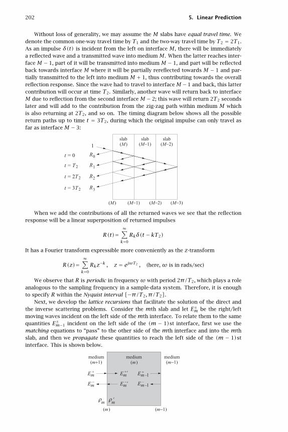
202 5. Linear Prediction
Without loss of generality, we may assume the M slabs have equal travel time. Wedenote the common one-way travel time by T1 and the two-way travel time by T2 = 2T1.As an impulse δ(t) is incident from the left on interface M, there will be immediatelya reflected wave and a transmitted wave into mediumM. When the latter reaches inter-face M − 1, part of it will be transmitted into medium M − 1, and part will be reflectedback towards interface M where it will be partially rereflected towards M − 1 and par-tially transmitted to the left into medium M + 1, thus contributing towards the overallreflection response. Since the wave had to travel to interfaceM−1 and back, this lattercontribution will occur at time T2. Similarly, another wave will return back to interfaceM due to reflection from the second interfaceM− 2; this wave will return 2T2 secondslater and will add to the contribution from the zig-zag path within medium M whichis also returning at 2T2, and so on. The timing diagram below shows all the possiblereturn paths up to time t = 3T2, during which the original impulse can only travel asfar as interfaceM − 3:
When we add the contributions of all the returned waves we see that the reflectionresponse will be a linear superposition of returned impulses
R(t)=∞∑k=0
Rkδ(t − kT2)
It has a Fourier transform expressible more conveniently as the z-transform
R(z)=∞∑k=0
Rkz−k , z = ejωT2 , (here,ω is in rads/sec)
We observe that R is periodic in frequencyω with period 2π/T2, which plays a roleanalogous to the sampling frequency in a sample-data system. Therefore, it is enoughto specify R within the Nyquist interval [−π/T2,π/T2].
Next, we develop the lattice recursions that facilitate the solution of the direct andthe inverse scattering problems. Consider the mth slab and let E±m be the right/leftmoving waves incident on the left side of themth interface. To relate them to the samequantities E±m−1 incident on the left side of the (m − 1)st interface, first we use thematching equations to “pass” to the other side of the mth interface and into the mthslab, and then we propagate these quantities to reach the left side of the (m − 1)stinterface. This is shown below.

5.13. Dynamic Predictive Deconvolution—Waves in Layered Media 203
The matching equations are:[E+mE−m
]= 1
tm
[1 ρmρm 1
][E+′mE−′m
], tm = (1− ρ2
m)1/2 (5.13.8)
Since the left-moving wave E−′m is the delayed replica of E−m−1 by T1 seconds, andE+′m is the advanced replica of E+m−1 by T1 seconds, it follows that
E+′m = z1/2E+m−1 , E−′m = z−1/2E−m−1
or, in matrix form [E+′mE−′m
]=
[z1/2 00 z−1/2
][E+m−1
E−m−1
](5.13.9)
where the variable z−1 was defined above and represents the two-way travel time delay,while z−1/2 represents the one-way travel time delay. Combining the matching andpropagation equations (5.13.8) and (5.13.9), we obtain the desired relationship betweenE±m and E±m−1: [
E+mE−m
]= z
1/2
tm
[1 ρmz−1
ρm z−1
][E+m−1
E−m−1
](5.13.10)
Or, written in a convenient vector notation
Em(z)= ψm(z)Em−1(z) (5.13.11)
where we defined
Em(z)=[E+m(z)E−m(z)
], ψm(z)= z
1/2
tm
[1 ρmz−1
ρm z−1
](5.13.12)
The “match-and-propagate” transition matrixψm(z) has two interesting properties;namely, defining ψm(z)= ψm(z−1)
ψm(z)TJ3ψm(z)= J3 , J3 =[
1 00 −1
](5.13.13)
ψm(z)= J1ψm(z)J1 , J1 =[
0 11 0
](5.13.14)
where J1, J3 are recognized as two of the three Pauli spin matrices. From Eq. (5.3.13),we have with E±m(z)= E±m(z−1):
E+mE+m − E−mE−m = ETmJ3Em = ETm−1ψTmJ3ψmEm−1 = ETm−1J3Em−1
= E+m−1E+m−1 − E−m−1E
−m−1
(5.13.15)
which is equivalent to energy conservation, according to Eq. (5.13.5). The second prop-erty, Eq. (5.13.14), expresses time-reversal invariance and allows the construction of asecond, linearly independent, solution of the recursive equations (5.13.11), Using theproperty J2
1 = I, we have
Em = J1Em =[E−mE+m
]= J1ψmEm−1 = J1ψmJ1J1Em−1 = ψmEm−1 (5.13.16)
The recursions (5.13.11) may be iterated now down to m = 0. By an additionalboundary match, we may pass to the right side of interfacem = 0:
Em = ψmψm−1 · · ·ψ1E0 = ψmψm−1 · · ·ψ1ψ0E′0

204 5. Linear Prediction
where we defined ψ0 by
ψ0 = 1
t0
[1 ρ0
ρ0 1
]or, more explicitly[
E+mE−m
]= zm/2
tmtm−1 · · · t1t0
[1 ρmz−1
ρm z−1
]· · ·
[1 ρ1z−1
ρ1 z−1
][1 ρ0
ρ0 1
][E+′0
E−′0
](5.13.17)
To deal with this product of matrices, we define[Am CmBm Dm
]=
[1 ρmz−1
ρm z−1
]· · ·
[1 ρ1z−1
ρ1 z−1
][1 ρ0
ρ0 1
](5.13.18)
where Am,Cm,Bm,Dm are polynomials of degree m in the variable z−1. The energyconservation and time-reversal invariance properties of the ψm matrices imply similarproperties for these polynomials. Writing Eq. (5.13.18) in terms of the ψms, we have[
Am CmBm Dm
]= z−m/2σmψmψm−1 · · ·ψ1ψ0
where we defined the quantity
σm = tmtm−1 · · · t1t0 =m∏i=0
(1− ρ2i )
1/2 (5.13.19)
Property (5.13.13) implies the same for the above product of matrices; that is, withAm(z)= Am(z−1), etc.,[
Am CmBm Dm
][1 00 −1
][Am CmBm Dm
]=
[1 00 −1
]σ2m
which implies that the quantity Am(z)Am(z)−Bm(z)Bm(z) is independent of z:
Am(z)Am(z)−Bm(z)Bm(z)= σ2m (5.13.20)
Property (5.13.14) implies that Cm and Dm are the reverse polynomials BRm and ARm,respectively; indeed[
ARm CRmBRm DRm
]= z−m
[Am CmBm Dm
]= z−mzm/2σmψm · · · ψ1ψ0
= z−m/2σmJ1(ψm · · ·ψ0)J1 = J1
[Am CmBm Dm
]J1
=[
0 11 0
][Am CmBm Dm
][0 11 0
]=
[Dm BmCm Am
](5.13.21)
from which it follows thatCm(z)= BRm(z) andDm(z)= ARm(z). The definition (5.13.18)implies also the recursion[
Am BRmBm ARm
]=
[1 ρmz−1
ρm z−1
][Am−1 BRm−1
Bm−1 ARm−1
]
Therefore each column of the ABCD matrix satisfies the same recursion. To sum-marize, we have[
Am(z) BRm(z)Bm(z) ARm(z)
]=
[1 ρmz−1
ρm z−1
]· · ·
[1 ρ1z−1
ρ1 z−1
][1 ρ0
ρ0 1
](5.13.22)

5.13. Dynamic Predictive Deconvolution—Waves in Layered Media 205
with the lattice recursion[Am(z)Bm(z)
]=
[1 ρmz−1
ρm z−1
][Am−1(z)Bm−1(z)
](5.13.23)
and the property (5.13.20). The lattice recursion is initialized atm = 0 by:
A0(z)= 1 , B0(z)= ρ0 , or,
[A0(z) BR0 (z)B0(z) AR0 (z)
]=
[1 ρ0
ρ0 1
](5.13.24)
Furthermore, it follows from the lattice recursion (5.13.23) that the reflection coeffi-cients ρm always appear in the first and last coefficients of the polynomials Am(z) andBm(z), as follows
am(0)= 1 , am(m)= ρ0ρm , bm(0)= ρm , bm(m)= ρ0 (5.13.25)
Eq. (5.13.17) for the field components reads now[E+mE−m
]= z
m/2
σm
[Am BRmBm ARm
][E+′0
E−′0
]
Settingm =M, we find the relationship between the fields incident on the dielectricslab structure from the left to those incident from the right:[
E+ME−M
]= z
M/2
σM
[AM BRMBM ARM
][E+′0
E−′0
](5.13.26)
All the multiple reflections and reverberatory effects of the structure are buried inthe transition matrix [
AM BRMBM ARM
]In reference to Fig. 5.14, the reflection and transmission responses R,T,R′, T′ of
the structure can be obtained from Eq. (5.13.26) by noting that[1R
]= z
M/2
σM
[AM BRMBM ARM
][T0
],
[0T′
]= z
M/2
σM
[AM BRMBM ARM
][R′
1
]
which may be combined into one equation:[1 0R T′
]= z
M/2
σM
[AM BRMBM ARM
][T R′
0 1
]
that can be written as follows:
zM/2
σM
[AM BRMBM ARM
]=
[1 0R T′
][T R′
0 1
]−1
=[
1 0R 1
][T−1 0
0 T′
][1 −R′0 1
]
Solving these for the reflection and transmission responses, we find:
R(z)= BM(z)AM(z)
, T(z)= σMz−M/2
AM(z)
R′(z)= −BRM(z)AM(z)
, T′(z)= σMz−M/2
AM(z)
(5.13.27)
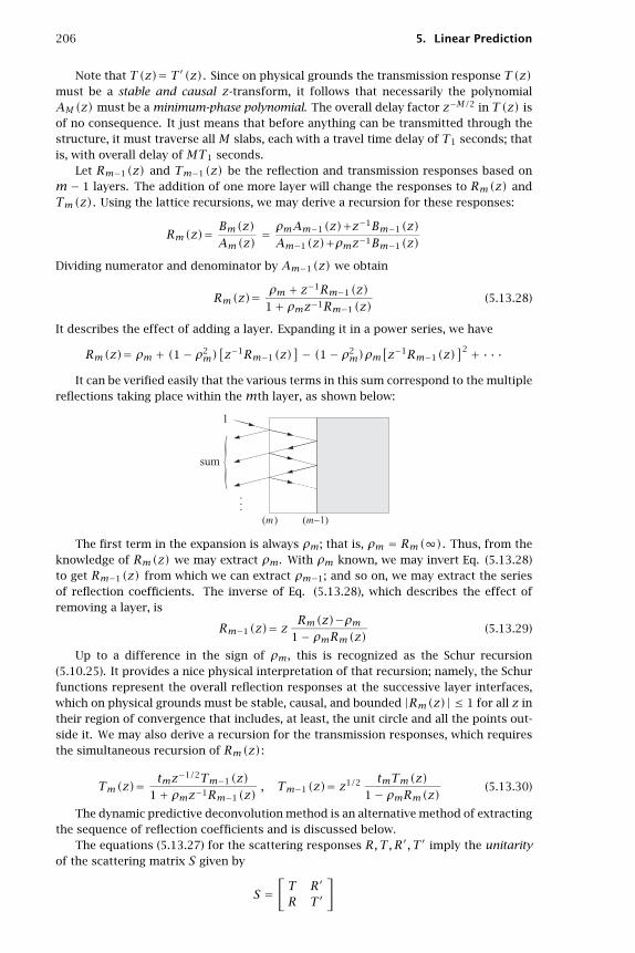
206 5. Linear Prediction
Note that T(z)= T′(z). Since on physical grounds the transmission response T(z)must be a stable and causal z-transform, it follows that necessarily the polynomialAM(z)must be a minimum-phase polynomial. The overall delay factor z−M/2 in T(z) isof no consequence. It just means that before anything can be transmitted through thestructure, it must traverse allM slabs, each with a travel time delay of T1 seconds; thatis, with overall delay ofMT1 seconds.
Let Rm−1(z) and Tm−1(z) be the reflection and transmission responses based onm − 1 layers. The addition of one more layer will change the responses to Rm(z) andTm(z). Using the lattice recursions, we may derive a recursion for these responses:
Rm(z)= Bm(z)Am(z)= ρmAm−1(z)+z−1Bm−1(z)Am−1(z)+ρmz−1Bm−1(z)
Dividing numerator and denominator by Am−1(z) we obtain
Rm(z)= ρm + z−1Rm−1(z)1+ ρmz−1Rm−1(z)
(5.13.28)
It describes the effect of adding a layer. Expanding it in a power series, we have
Rm(z)= ρm + (1− ρ2m)
[z−1Rm−1(z)
]− (1− ρ2m)ρm
[z−1Rm−1(z)
]2 + · · ·It can be verified easily that the various terms in this sum correspond to the multiple
reflections taking place within themth layer, as shown below:
The first term in the expansion is always ρm; that is, ρm = Rm(∞). Thus, from theknowledge of Rm(z) we may extract ρm. With ρm known, we may invert Eq. (5.13.28)to get Rm−1(z) from which we can extract ρm−1; and so on, we may extract the seriesof reflection coefficients. The inverse of Eq. (5.13.28), which describes the effect ofremoving a layer, is
Rm−1(z)= z Rm(z)−ρm1− ρmRm(z) (5.13.29)
Up to a difference in the sign of ρm, this is recognized as the Schur recursion(5.10.25). It provides a nice physical interpretation of that recursion; namely, the Schurfunctions represent the overall reflection responses at the successive layer interfaces,which on physical grounds must be stable, causal, and bounded |Rm(z)| ≤ 1 for all z intheir region of convergence that includes, at least, the unit circle and all the points out-side it. We may also derive a recursion for the transmission responses, which requiresthe simultaneous recursion of Rm(z):
Tm(z)= tmz−1/2Tm−1(z)1+ ρmz−1Rm−1(z)
, Tm−1(z)= z1/2 tmTm(z)1− ρmRm(z) (5.13.30)
The dynamic predictive deconvolution method is an alternative method of extractingthe sequence of reflection coefficients and is discussed below.
The equations (5.13.27) for the scattering responses R,T,R′, T′ imply the unitarityof the scattering matrix S given by
S =[T R′
R T′
]

5.13. Dynamic Predictive Deconvolution—Waves in Layered Media 207
that is,S(z)TS(z)= S(z−1)TS(z)= I (5.13.31)
where I is the 2×2 unit matrix. On the unit circle z = ejωT2 the scattering matrixbecomes a unitary matrix: S(ω)†S(ω)= I. Component-wise, Eq. (5.13.3 1 ) becomes
TT + RR = T′T′ + R′R′ = 1 , TR′ + RT′ = 0 (5.13.32)
Robinson and Treitel’s dynamic predictive deconvolution method [59] of solving theinverse scattering problem is based on the above unitarity equation. In the inverseproblem, it is required to extract the set of reflection coefficients from measurements ofeither the reflection response R or the transmission response T. In speech processing itis the transmission response that is available. In geophysical applications, or in studyingthe reflectivity properties of thin films, it is the reflection response that is available. Theproblem of designing terminations of transmission lines also falls in the latter category.In this case, an appropriate termination is desired that must have a specified reflectionresponse R(z); for example, to be reflectionless over a wide band of frequencies aboutsome operating frequency.
The solution of both types of problems follows the same steps. First, from theknowledge of the reflection response R(z), or the transmission response T(z), thespectral function of the structure is defined:
Φ(z)= 1−R(z)R(z)= T(z)T(z)= σ2M
AM(z)AM(z)(5.13.33)
This is recognized as the power spectrum of the transmission response, and it is ofthe autoregressive type. Thus, linear prediction methods can be used in the solution.
In the time domain, the autocorrelation lags φ(k) of the spectral function are ob-tained from the sample autocorrelations of the reflection sequence, or the transmissionsequence:
φ(k)= δ(k)−C(k)= D(k) (5.13.34)
whereC(k) andD(k) are the sample autocorrelations of the reflection and transmissiontime responses:
C(k)=∑nR(n+ k)R(n) , D(k)=
∑nT(n+ k)T(n) (5.13.35)
In practice, only a finite record of the reflection (or transmission) sequence will beavailable, say {R(0),R(1), . . . , R(N − 1)}. Then, an approximation to C(k) must beused, as follows:
C(k)=N−1−k∑n=0
R(n+ k)R(n) , k = 0,1, . . . ,M (5.13.36)
The polynomial AM(z) may be recovered from the knowledge of the firstM lags ofthe spectral function; that is, {φ(0),φ(1), . . . ,φ(M)}. The determining equations forthe coefficients of AM(z) are precisely the normal equations of linear prediction. In thepresent context, they may be derived directly by noting that Φ(z) is a stable spectraldensity and is already factored into its minimum-phase factors in Eq. (5.13.33). Thus,writing
Φ(z)AM(z)= σ2M
AM(z−1)it follows that the right-hand side is expandable in positive powers of z; the negativepowers of z in the left-hand side must be set equal to zero. This gives the normal

208 5. Linear Prediction
equations:⎡⎢⎢⎢⎢⎢⎢⎢⎣
φ(0) φ(1) φ(2) · · · φ(M)φ(1) φ(0) φ(1) · · · φ(M − 1)φ(2) φ(1) φ(0) · · · φ(M − 2)
......
......
φ(M) φ(M − 1) φ(M − 2) · · · φ(0)
⎤⎥⎥⎥⎥⎥⎥⎥⎦
⎡⎢⎢⎢⎢⎢⎢⎢⎣
1aM(1)aM(2)
...aM(M)
⎤⎥⎥⎥⎥⎥⎥⎥⎦ =⎡⎢⎢⎢⎢⎢⎢⎢⎣
σ2M00...0
⎤⎥⎥⎥⎥⎥⎥⎥⎦ (5.13.37)
which can be solved efficiently using Levinson’s algorithm. Having obtained AM(z)and noting the BM(z)= AM(z)R(z), the coefficients of the polynomial BM(z) may berecovered by convolution:
bM(n)=n∑m=0
aM(n−m)R(m) , n = 0,1, . . . ,M (5.13.38)
Having obtained both AM(z) and BM(z) and noting that ρM = bM(0), the latticerecursion (5.13.23) may be inverted to recover the polynomials AM−1(z) and BM−1(z)as well as the next reflection coefficient ρM−1 = bM−1(0), and so on. The inverse of thelattice recursion matrix is[
1 ρmz−1
ρm z−1
]−1
= 1
1− ρ2m
[1 −ρm
−ρmz z
]
Therefore, the backward recursion becomes:
ρm = bm(0) ,[Am−1(z)Bm−1(z)
]= 1
1− ρ2m
[1 −ρm
−ρmz z
][Am(z)Bm(z)
](5.13.39)
In this manner, all the reflection coefficients {ρ0, ρ1, . . . , ρM} can be extracted. Thecomputational algorithm is summarized as follows:
1. Measure R(0),R(1), . . . , R(N − 1).2. Select a reasonable value for the number of slabsM.
3. Compute the M + 1 sample autocorrelation lags C(0),C(1), . . . , C(M) of the re-flection response R(n), using Eq. (5.13.36).
4. Compute φ(k)= δ(k)−C(k), k = 0,1, . . . ,M.
5. Using Levinson’s algorithm, solve the normal equations (5.13.37) for the coeffi-cients of AM(z).
6. Convolve AM(z) with R(z) to find BM(z).7. Compute ρM = bM(0) and iterate the backward recursion (5.13.39) fromm =M
down tom = 0.
The subroutine dpd (see Appendix B) is an implementation of the dynamic predictivedeconvolution procedure. The inputs to the subroutine are N samples of the reflectionresponse {R(0),R(1), . . . , R(N − 1)} and the number of layers M. The outputs arethe lattice polynomials Ai(z) and Bi(z), for i = 0,1, . . . ,M, arranged in the two lower-triangular matricesA and B whose rows hold the coefficients of these polynomials; thatis, A(i, j)= ai(j), or
Ai(z)=i∑j=0
A(i, j)z−j
and similarly for Bi(z). The subroutine invokes the routine lev to solve the normalequations (5.13.34). The forward scattering problem is implemented by the subroutinescatter, whose inputs are the set of reflection coefficients {ρ0, ρ1, . . . , ρM} and whose
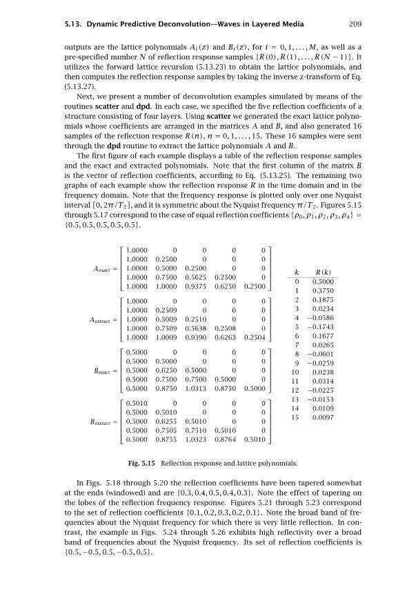
5.13. Dynamic Predictive Deconvolution—Waves in Layered Media 209
outputs are the lattice polynomials Ai(z) and Bi(z), for i = 0,1, . . . ,M, as well as apre-specified number N of reflection response samples {R(0),R(1), . . . , R(N − 1)}. Itutilizes the forward lattice recursion (5.13.23) to obtain the lattice polynomials, andthen computes the reflection response samples by taking the inverse z-transform of Eq.(5.13.27).
Next, we present a number of deconvolution examples simulated by means of theroutines scatter and dpd. In each case, we specified the five reflection coefficients of astructure consisting of four layers. Using scatter we generated the exact lattice polyno-mials whose coefficients are arranged in the matrices A and B, and also generated 16samples of the reflection response R(n), n = 0,1, . . . ,15. These 16 samples were sentthrough the dpd routine to extract the lattice polynomials A and B.
The first figure of each example displays a table of the reflection response samplesand the exact and extracted polynomials. Note that the first column of the matrix Bis the vector of reflection coefficients, according to Eq. (5.13.25). The remaining twographs of each example show the reflection response R in the time domain and in thefrequency domain. Note that the frequency response is plotted only over one Nyquistinterval [0,2π/T2], and it is symmetric about the Nyquist frequencyπ/T2. Figures 5.15through 5.17 correspond to the case of equal reflection coefficients {ρ0, ρ1, ρ2, ρ3, ρ4} ={0.5,0.5,0.5,0.5,0.5}.
Aexact =
⎡⎢⎢⎢⎢⎢⎢⎣1.0000 0 0 0 01.0000 0.2500 0 0 01.0000 0.5000 0.2500 0 01.0000 0.7500 0.5625 0.2500 01.0000 1.0000 0.9375 0.6250 0.2500
⎤⎥⎥⎥⎥⎥⎥⎦
Aextract =
⎡⎢⎢⎢⎢⎢⎢⎣1.0000 0 0 0 01.0000 0.2509 0 0 01.0000 0.5009 0.2510 0 01.0000 0.7509 0.5638 0.2508 01.0000 1.0009 0.9390 0.6263 0.2504
⎤⎥⎥⎥⎥⎥⎥⎦
Bexact =
⎡⎢⎢⎢⎢⎢⎢⎣0.5000 0 0 0 00.5000 0.5000 0 0 00.5000 0.6250 0.5000 0 00.5000 0.7500 0.7500 0.5000 00.5000 0.8750 1.0313 0.8750 0.5000
⎤⎥⎥⎥⎥⎥⎥⎦
Bextract =
⎡⎢⎢⎢⎢⎢⎢⎣0.5010 0 0 0 00.5000 0.5010 0 0 00.5000 0.6255 0.5010 0 00.5000 0.7505 0.7510 0.5010 00.5000 0.8755 1.0323 0.8764 0.5010
⎤⎥⎥⎥⎥⎥⎥⎦
k R(k)0 0.50001 0.37502 0.18753 0.02344 −0.05865 −0.17436 0.16777 0.02658 −0.06019 −0.0259
10 0.023811 0.031412 −0.022513 −0.015314 0.010915 0.0097
Fig. 5.15 Reflection response and lattice polynomials.
In Figs. 5.18 through 5.20 the reflection coefficients have been tapered somewhatat the ends (windowed) and are {0.3,0.4,0.5,0.4,0.3}. Note the effect of tapering onthe lobes of the reflection frequency response. Figures 5.21 through 5.23 correspondto the set of reflection coefficients {0.1,0.2,0.3,0.2,0.1}. Note the broad band of fre-quencies about the Nyquist frequency for which there is very little reflection. In con-trast, the example in Figs. 5.24 through 5.26 exhibits high reflectivity over a broadband of frequencies about the Nyquist frequency. Its set of reflection coefficients is{0.5,−0.5,0.5,−0.5,0.5}.

210 5. Linear Prediction
0 2 4 6 8 10 12 14−0.2
−0.1
0
0.1
0.2
0.3
0.4
0.5
0.6
time k
time response R(k)
0 0.2 0.4 0.6 0.8 10
0.2
0.4
0.6
0.8
1
frequency in cycles/sample
frequency response |R(ω )|2
Fig. 5.16 and Fig. 5.17 Reflection responses in the time and frequency domains.
Aexact =
⎡⎢⎢⎢⎢⎢⎢⎣1.0000 0 0 0 01.0000 0.1200 0 0 01.0000 0.3200 0.1500 0 01.0000 0.5200 0.3340 0.1200 01.0000 0.6400 0.5224 0.2760 0.0900
⎤⎥⎥⎥⎥⎥⎥⎦
Aextract =
⎡⎢⎢⎢⎢⎢⎢⎣1.0000 0 0 0 01.0000 0.1200 0 0 01.0000 0.3200 0.1500 0 01.0000 0.5200 0.3340 0.1200 01.0000 0.6400 0.5224 0.2760 0.0900
⎤⎥⎥⎥⎥⎥⎥⎦
Bexact =
⎡⎢⎢⎢⎢⎢⎢⎣0.3000 0 0 0 00.4000 0.3000 0 0 00.5000 0.4600 0.3000 0 00.4000 0.6280 0.5200 0.3000 00.3000 0.5560 0.7282 0.5560 0.3000
⎤⎥⎥⎥⎥⎥⎥⎦
Bextract =
⎡⎢⎢⎢⎢⎢⎢⎣0.3000 0 0 0 00.4000 0.3000 0 0 00.5000 0.4600 0.3000 0 00.4000 0.6280 0.5200 0.3000 00.3000 0.5560 0.7282 0.5560 0.3000
⎤⎥⎥⎥⎥⎥⎥⎦
k R(k)0 0.30001 0.36402 0.33853 0.06644 −0.04685 −0.13096 0.05947 0.03738 −0.01469 −0.0148
10 0.001411 0.007512 −0.000113 −0.002914 −0.000315 0.0010
Fig. 5.18 Reflection response and lattice polynomials.
In this section we have discussed the inverse problem of unraveling the structureof a medium from the knowledge of its reflection response. The connection of the dy-namic predictive deconvolution method to the conventional inverse scattering meth-ods based on the Gelfand-Levitan-Marchenko approach [139] has been discussed in[128,140,141]. The lattice recursions characteristic of the wave propagation problemwere derived as a direct consequence of the boundary conditions at the interfaces be-tween media, whereas the lattice recursions of linear prediction were a direct conse-quence of the Gram-Schmidt orthogonalization process and the minimization of theprediction-error performance index. Is there a deeper connection between these twoproblems [76,79,80,90–92,142,143]? One notable result in this direction has been toshow that the Cholesky factorization of Toeplitz or near-Toeplitz matrices via the Schuralgorithm can be cast in a wave propagation model and derived as a simple consequenceof energy conservation [87].

5.14. Least-Squares Waveshaping and Spiking Filters 211
0 2 4 6 8 10 12 14−0.2
−0.1
0
0.1
0.2
0.3
0.4
time k
time response R(k)
0 0.2 0.4 0.6 0.8 10
0.2
0.4
0.6
0.8
1
frequency in cycles/sample
frequency response |R(ω )|2
Fig. 5.19 and Fig. 5.20 Reflection responses in the time and frequency domains.
Aexact =
⎡⎢⎢⎢⎢⎢⎢⎣1.0000 0 0 0 01.0000 0.0200 0 0 01.0000 0.0800 0.0300 0 01.0000 0.1400 0.0712 0.0200 01.0000 0.1600 0.1028 0.0412 0.0100
⎤⎥⎥⎥⎥⎥⎥⎦
Aextract =
⎡⎢⎢⎢⎢⎢⎢⎣1.0000 0 0 0 01.0000 0.0200 0 0 01.0000 0.0800 0.0300 0 01.0000 0.1400 0.0712 0.0200 01.0000 0.1600 0.1028 0.0412 0.0100
⎤⎥⎥⎥⎥⎥⎥⎦
Bexact =
⎡⎢⎢⎢⎢⎢⎢⎣0.1000 0 0 0 00.2000 0.1000 0 0 00.3000 0.2060 0.1000 0 00.2000 0.3160 0.2120 0.1000 00.1000 0.2140 0.3231 0.2140 0.1000
⎤⎥⎥⎥⎥⎥⎥⎦
Bextract =
⎡⎢⎢⎢⎢⎢⎢⎣0.1000 0 0 0 00.2000 0.1000 0 0 00.3000 0.2060 0.1000 0 00.2000 0.3160 0.2120 0.1000 00.1000 0.2140 0.3231 0.2140 0.1000
⎤⎥⎥⎥⎥⎥⎥⎦
k R(k)0 0.10001 0.19802 0.28123 0.14454 0.03885 −0.03466 −0.00727 0.00178 0.00159 0.0002
10 −0.000211 −0.000112 0.000013 0.000014 0.000015 −0.0000
Fig. 5.21 Reflection response and lattice polynomials.
5.14 Least-Squares Waveshaping and Spiking Filters
In linear prediction, the three practical methods of estimating the prediction error filtercoefficients were all based on replacing the ensemble mean-square minimization crite-rion by a least-squares criterion based on time averages. Similarly, the more generalWiener filtering problem may be recast in terms of such time averages. A practical for-mulation, which is analogous to the Yule-Walker or autocorrelation method, is as follows[59,60,95,144]. Given a record of available data
y0, y1, . . . , yN
find the best linear FIR filter of orderM
h0, h1, . . . , hM

212 5. Linear Prediction
0 2 4 6 8 10 12 14−0.1
−0.05
0
0.05
0.1
0.15
0.2
0.25
0.3
time k
time response R(k)
0 0.2 0.4 0.6 0.8 10
0.2
0.4
0.6
0.8
1
frequency in cycles/sample
frequency response |R(ω )|2
Fig. 5.22 and Fig. 5.23 Reflection responses in the time and frequency domains.
Aexact =
⎡⎢⎢⎢⎢⎢⎢⎣1.0000 0 0 0 01.0000 −0.2500 0 0 01.0000 −0.5000 0.2500 0 01.0000 −0.7500 0.5625 −0.2500 01.0000 −1.0000 0.9375 −0.6250 0.2500
⎤⎥⎥⎥⎥⎥⎥⎦
Aextract =
⎡⎢⎢⎢⎢⎢⎢⎣1.0000 0 0 0 01.0000 −0.2509 0 0 01.0000 −0.5009 0.2510 0 01.0000 −0.7509 0.5638 −0.2508 01.0000 −1.0009 0.9390 −0.6263 0.2504
⎤⎥⎥⎥⎥⎥⎥⎦
Bexact =
⎡⎢⎢⎢⎢⎢⎢⎣0.5000 0 0 0 0−0.5000 0.5000 0 0 0
0.5000 −0.6250 0.5000 0 0−0.5000 0.7500 −0.7500 0.5000 0
0.5000 −0.8750 1.0313 −0.8750 0.5000
⎤⎥⎥⎥⎥⎥⎥⎦
Bextract =
⎡⎢⎢⎢⎢⎢⎢⎣0.5010 0 0 0 0−0.5000 0.5010 0 0 0
0.5000 −0.6255 0.5010 0 0−0.5000 0.7505 −0.7510 0.5010 0
0.5000 −0.8755 1.0323 −0.8764 0.5010
⎤⎥⎥⎥⎥⎥⎥⎦
k R(k)0 0.50001 −0.37502 0.18753 −0.02344 −0.05865 0.17436 0.16777 −0.02658 −0.06019 0.0259
10 0.023811 −0.031412 −0.022513 0.015314 0.010915 −0.0097
Fig. 5.24 Reflection response and lattice polynomials.
which reshapes yn into a desired signal xn, specified in terms of the samples:
x0, x1, . . . , xN+M
where for consistency of convolution, we assumed we know N +M + 1 samples of thedesired signal. The actual convolution output of the waveshaping filter will be:
xn =min(n,M)∑
m=max(0,n−N)hmxn−m , 0 ≤ n ≤ N +M (5.14.1)
and the estimation error:
en = xn − xn , 0 ≤ n ≤ N +M (5.14.2)

5.14. Least-Squares Waveshaping and Spiking Filters 213
0 2 4 6 8 10 12 14−0.6
−0.4
−0.2
0
0.2
0.4
0.6
time k
time response R(k)
0 0.2 0.4 0.6 0.8 10
0.2
0.4
0.6
0.8
1
frequency in cycles/sample
frequency response |R(ω )|2
Fig. 5.25 and Fig. 5.26 Reflection responses in the time and frequency domains.
As the optimality criterion, we choose the least-squares criterion:
E =N+M∑n=0
e2n = min (5.14.3)
The optimal filter weights hm are selected to minimize E. It is convenient to recastthe above in a compact matrix form. Define the (N+M+1)×(M+1) convolution datamatrix Y, the (M+1)×1 vector of filter weights h, the (N+M+1)×1 vector of desiredsamples x, (and estimates x and estimation errors e), as follows:
Y =
⎡⎢⎢⎢⎢⎢⎢⎢⎢⎢⎢⎢⎢⎢⎢⎢⎢⎢⎢⎣
y0 0 0 · · · 0y1 y0 0 · · · 0y2 y1 y0 · · · 0...
......
...yN yN−1 yN−2 · · · yN−M0 yN yN−1 · · · yN−M+1
0 0 yN · · · yN−M+2
......
......
0 0 0 · · · yN
⎤⎥⎥⎥⎥⎥⎥⎥⎥⎥⎥⎥⎥⎥⎥⎥⎥⎥⎥⎦
, h =
⎡⎢⎢⎢⎢⎢⎣h0
h1
...hM
⎤⎥⎥⎥⎥⎥⎦ , x =
⎡⎢⎢⎢⎢⎢⎣x0
x1
...xN+M
⎤⎥⎥⎥⎥⎥⎦ (5.14.4)
Equations (5.14.1) through (5.14.3) now become
x = Yh , e = x− x , E = eTe (5.14.5)
Minimizing E with respect to the weight vector h results in the orthogonality equations:
YTe = YT(x−Yh)= 0 (5.14.6)
which are equivalent to the normal equations:
YTYh = YTx (5.14.7)
Solving for h, we findh = (YTY)−1YTx = R−1r (5.14.8)
where the quantitiesR = YTY , r = YTx (5.14.9)
may be recognized (see Section 1.10) as the (M + 1)×(M + 1) autocorrelation matrixformed by the sample autocorrelations Ryy(0), Ryy(1), . . . Ryy(M) of yn, and as the

214 5. Linear Prediction
(M+1)×1 vector of sample cross-correlations Rxy(0), Rxy(1), . . . Rxy(M) between thedesired and the available vectors xn and yn. We have already used this expression forthe weight vector h in the example of Section 5.11. Here we have justified it in termsof the least-squares criterion (5.14.3). The subroutine firw may be used to solve for theweights (5.14.8) and, if so desired, to give the corresponding lattice realization. Theactual filter output x is expressed as
x = Yh = YR−1YTx = Px (5.14.10)
whereP = YR−1YT = Y(YTY)−1YT (5.14.11)
The error vector becomes e = (I − P)x. The “performance” matrix P is a projectionmatrix, and thus, so is (I − P). Then, the error square becomes
E = eTe = xT(I − P)2x = xT(I − P)x (5.14.12)
The (N+M+1)×(N+M+1)matrix P has trace equal toM+1, as can be checkedeasily. Since its eigenvalues as a projection matrix are either 0 or 1, it follows that inorder for the sum of all the eigenvalues (the trace) to be equal to M + 1, there mustnecessarily be M + 1 eigenvalues that are equal to 1, and N eigenvalues equal to 0.Therefore, the matrix P has rankM+ 1, and if the desired vector x is selected to be anyof theM+1 eigenvectors belonging to eigenvalue 1, the corresponding estimation errorwill be zero.
Among all possible waveshapes that may be chosen for the desired vector x, ofparticular importance are the spikes, or impulses. In this case, x is a unit impulse, sayat the origin; that is, xn = δn. The convolution xn = hn ∗ yn of the corresponding filterwith yn is the best least-squares approximation to the unit impulse. In other words, hn isthe best least-squares inverse filter to yn that attempts to reshape, or compress, yn intoa unit impulse. Such least squares inverse filters are used extensively in deconvolutionapplications. More generally. the vector x may be chosen to be any one of the unitvectors
x = ui =
⎡⎢⎢⎢⎢⎢⎢⎢⎢⎢⎢⎢⎢⎢⎣
0...010...0
⎤⎥⎥⎥⎥⎥⎥⎥⎥⎥⎥⎥⎥⎥⎦← ith slot , i = 0,1, . . . ,N +M (5.14.13)
which corresponds to a unit impulse occurring at the ith time instant instead of at theorigin; that is, xn = δ(n− i). The actual output from the spiking filter is given by
x = Px = Pui = ith column of P (5.14.14)
Thus, the ith column of the matrix P is the output of the ith spiking filter whichattempts to compress yn into a spike with i delays. The corresponding ith filter ish = R−1YTui. Therefore, the columns of the matrix
H = R−1YT = (YTY)−1YT (5.14.15)
are all the optimal spiking filters. The estimation error of the ith filter is
Ei = uTi (I − P)ui = 1− Pii (5.14.16)

5.14. Least-Squares Waveshaping and Spiking Filters 215
where Pii, is the ith diagonal element of P. Since the delay imay be positioned anywherefrom i = 0 to i = N +M, there are N +M + 1 such spiking filters, each with error Ei.Among these, there will be one that has the optimal delay i which corresponds to thesmallest of the Eis; or, equivalently, to the maximum of the diagonal elements Pii.
The design procedure for least-squares spiking filters for a given finite signal yn,n = 0,1, . . . ,N − 1 is summarized as follows:
1. Compute R = YTY.
2. Compute the inverse R−1 (preferably by the Levinson recursion).
3. Compute H = R−1YT = all the spiking filters.
4. Compute P = YH = YR−1YT = all spiking filter outputs.
5. Select that column i of P for which Pii is the largest.
If the Levinson-Cholesky algorithm is used to compute the inverse R−1, this designprocedure becomes fairly efficient. An implementation of the procedure is given by thesubroutine spike. The inputs to the subroutine are the N + 1 samples {y0, y1, . . . , yN},the desired order M of the spiking filter, and a so-called “prewhitening” or Backus-Gilbert parameter ε, which will be explained below. The outputs of the subroutine arethe matrices P and H.
To explain the role of the parameter ε, let us go back to the waveshaping problem.When the data sequence yn to be reshaped into xn is inaccurately known—if, for example,it has been contaminated by white noise vn—the least-squares minimization criterion(5.14.3) can be extended slightly to accomplish the double task of (1) producing thebest estimate of xn and (2) reducing the noise at the output of the filter hn as much aspossible.
The input to the filter is the noisy sequence yn+vn and its output is hn∗yn+hn∗vn = xn + un, where we set un = hn ∗ vn. The term un represents the filtered noise.The minimization criterion (5.14.3) may be replaced by
E =∑ne2n + λE[u2
n]= min (5.14.17)
where λ is a positive parameter which can be chosen by the user. Large λ emphasizeslarge reduction of the output noise, but this is done at the expense of resolution; that is,at the expense of obtaining a very good estimate. On the other hand, small λ emphasizeshigher resolution but with lesser noise reduction. This tradeoff between resolution andnoise reduction is the basic property of this performance index. Assuming that vn iswhite with variance σ2
v , we have
E[u2n]= σ2
v
M∑n=0
h2n = σ2
v hTh
Thus, Eq. (5.14.17) may be written as
E = eTe+ λσ2v hTh = min (5.14.18)
Its minimization with respect to h gives the normal equations:
(YTY + λσ2v I)h = YTx (5.14.19)
from which it is evident that the diagonal of YTY is shifted by an amount λσ2v ; that is,
Ryy(0)−→ Ryy(0)+λσ2v ≡ (1+ ε)Ryy(0) , ε = λσ2
v
Ryy(0)

216 5. Linear Prediction
In practice, εmay be taken to be a few percent or less. It is evident from Eq. (5.14.19)that one beneficial effect of the parameter ε is the stabilization of the inverse of thematrix YTY + λσ2
v I.The main usage of spiking filters is in deconvolution problems [59,60,95,144–146],
where the desired and the available signals xn and yn are related to each other by theconvolutional relationship
yn = fn ∗ xn =∑mfmxn−m (5.14.20)
where fn is a “blurring” function which is assumed to be approximately known. The ba-sic deconvolution problem is to recover xn from yn if fn is known. For example, yn mayrepresent the image of an object xn recorded through an optical system with a point-spread function fn. Or, yn might represent the recorded seismic trace arising from theexcitation of the layered earth by an impulsive waveform fn (the source wavelet) whichis convolved with the reflection impulse response xn of the earth (in the previous sec-tion xn was denoted by Rn.) If the effect of the source wavelet fn can be “deconvolvedaway,” the resulting reflection sequence xn may be subjected to the dynamic predictivedeconvolution procedure to unravel the earth structure. Or, fn may represent the im-pulse response of a channel, or a magnetic recording medium, which broadens and blurs(intersymbol interference) the desired message xn.
The least-squares inverse spiking filters offer a way to solve the deconvolution prob-lem: Simply design a least-squares spiking filter hn corresponding to the blurring func-tion fn; that is, hn ∗ fn � δn, in the least-squares sense. Then, filtering yn through hnwill recover the desired signal xn:
xn = hn ∗ yn = (hn ∗ fn)∗xn � δn ∗ xn = xn (5.14.21)
If the ith spiking filter is used, which compresses fn into an impulse with i delays,hn ∗ fn � δ(n− i), then the desired signal xn will be recovered with a delay of i unitsof time.
This and all other approaches to deconvolution work well when the data yn are notnoisy. In presence of noise, Eq. (5.14.20) becomes
yn = fn ∗ xn + vn (5.14.22)
where vn may be assumed to be zero-mean white noise of variance σ2v . Even if the
blurring function fn is known exactly and a good least-squares inverse filter hn can bedesigned, the presence of the noise term can distort the deconvolved signal beyondrecognition. This may be explained as follows. Filtering yn through the inverse filter hnresults in
hn ∗ yn = (hn ∗ fn)∗xn + hn ∗ vn � xn + unwhere un = hn ∗ vn is the filtered noise. Its variance is
E[u2n]= σ2
v hTh = σ2v
M∑n=0
h2n
which, depending on the particular shape of hn may be much larger than the originalvariance σ2
v . This happens, for example, when fn consists mainly of low frequencies.For hn to compress fn into a spike with a high frequency content, the impulse responsehn itself must be very spiky, which can result in values for hTh which are greater thanone.
To combat the effects of noise, the least-squares design criterion for h must bechanged by adding to it a term λE[u2
n] as was done in Eq. (5.14.17). The modified

5.14. Least-Squares Waveshaping and Spiking Filters 217
design criterion is then
E =∑n(δn − hn ∗ fn)2+λσ2
v
M∑n=0
h2n
which effectively amounts to changing the autocorrelation lag Rff (0) into (1+ε)Rff (0).The first term in this performance index tries to produce a good inverse filter; the secondterm tries to minimize the output power of the noise after filtering by the deconvolu-tion filter hn. Note that conceptually this index is somewhat different from that of Eq.(5.14.17), because now vn represents the noise in the data yn whereas there vn repre-sented inaccuracies in the knowledge of the wavelet fn.
In this approach to deconvolution we are not attempting to determine the best least-squares estimate of the desired signal xn, but rather the best least-squares inverse tothe blurring function fn. If the second order statistics of xn were known, we could, ofcourse, determine the optimal (Wiener) estimate xn of xn. This is also done in manyapplications.
The performance of the spiking filters and their usage in deconvolution are illus-trated by the following example: The blurring function fn to be spiked was chosen as
fn =⎧⎨⎩g(n− 25), n = 0,1, . . . ,65
0, for other n
where g(k) was the “gaussian hat” function:
g(k)= cos(0.15k)exp(−0.004k2)
The signal xn to be recovered was taken to be the series of delayed spikes:
xn =9∑i=0
aiδ(n− ni)
where the amplitudes ai and delays ni were chosen as
ai = 1, 0.8, 0.5, 0.95, 0.7, 0.5, 0.3, 0.9, 0.5, 0.85
ni = 25, 50, 60, 70, 80, 90, 100, 120, 140, 160
for i = 0,1,2,3,4,5,6,7,8,9.Figure 5.27 shows the signal fn to be spiked. Since the gaussian hat is symmetric
about the origin, we chose the spiking delay to be at i = 25. The order of the spikingfilter hn wasM = 50. Figure 5.28 shows the impulse response hn versus time. Note thespiky nature of hn which is required here because fn has a fairly low frequency content.Figure 5.29 shows the results of the convolution hn∗ fn, which is the best least-squaresapproximation to the impulse δ(n− 25).
The “goodness” of the spiking filter is judged by the diagonal entries of the per-formance matrix P, according to Eq. (5.14.16). For the chosen delay k = 25, we findP(25,25)= 0.97. To obtain a better picture of the overall performance of the spikingfilters, in Fig. 5.30 we have plotted the diagonal elements P(k, k) versus k. It is seenthat the chosen delay k = 25 is nearly optimal. Figure 5.31 shows the composite signalyn obtained by convolving fn and xn, according to Eq. (5.4.20).
Figure 5.32 shows the deconvolved signal xn according to Eq. (5.14.21). The recoveryof the amplitudes ai and delays ni of xn is very accurate. These results represent theidealistic case of noise-free data yn and perfect knowledge of the blurring function fn.To study the sensitivity of the deconvolution technique to inaccuracies in the knowledgeof the signal fn we have added a small high frequency perturbation on fn as follows:
f ′n = fn + 0.05 sin(1.5(n− 25)
)

218 5. Linear Prediction
0 20 40 60 80 100 120 140 160 180 200−0.4
−0.2
0
0.2
0.4
0.6
0.8
1
time samples
signal to be spiked
0 20 40 60 80 100 120 140 160 180 200−20
−15
−10
−5
0
5
10
15
20
time samples
impulse response of spiking filter
spiking delay = 25
Fig. 5.27 and Fig. 5.28 Reflection responses in the time and frequency domains.
0 20 40 60 80 100 120 140 160 180 200−0.4
−0.2
0
0.2
0.4
0.6
0.8
1
time samples
spiked signal, spiking delay = 25
spiked signaloriginal
0 20 40 60 80 100 120 140 160 180 2000
20
40
60
80
100
spiking delay position k
perc
ent
performance index P (k,k)
Fig. 5.29 and Fig. 5.30 Reflection responses in the time and frequency domains.
0 20 40 60 80 100 120 140 160 180 200−0.4
−0.2
0
0.2
0.4
0.6
0.8
1
time samples
composite signal
0 20 40 60 80 100 120 140 160 180 200−0.4
−0.2
0
0.2
0.4
0.6
0.8
1
time samples
deconvolution of composite signal
deconvolvedcomposite
Fig. 5.31 and Fig. 5.32 Reflection responses in the time and frequency domains.
The approximate signal f ′n is shown in Fig. 5.33. The spiking filter was designedon the basis of f ′n rather than fn. The result of filtering the same composite signal ynthrough the corresponding inverse filter is shown in Fig. 5.34. The delays and am-plitudes ai and ni are not well resolved, but the basic nature of xn can still be seen.Inspecting Fig. 5.28 we note the large spikes that are present in the impulse responsehn; these can cause the amplification of any additive noise component. Indeed, thenoise reduction ratio of the filter hn is hTh = 612, thus it will tend to amplify even

5.14. Least-Squares Waveshaping and Spiking Filters 219
0 20 40 60 80 100 120 140 160 180 200−0.4
−0.2
0
0.2
0.4
0.6
0.8
1
time samples
approximate signal
0 20 40 60 80 100 120 140 160 180 200−0.4
−0.2
0
0.2
0.4
0.6
0.8
1
time samples
deconvolution based on approximate signal
deconvolvedcomposite
Fig. 5.33 and Fig. 5.34 Reflection responses in the time and frequency domains.
small amounts of noise.To study the effect of noise, we have added a noise term vn, as in Eq. (5.14.22), with
variance equal to 10−4 (this corresponds to just 1% of the amplitude a0); the compositesignal yn is shown in Fig. 5.35. One can barely see the noise. Yet, after filtering withthe inverse filter hn of Fig. 5.28, the noise component is amplified to a great extent.The result of deconvolving the noisy yn with hn is shown in Fig. 5.36. To reduce theeffects of noise, the prewhitening parameter ε must be chosen to be nonzero. Even asmall nonzero value of ε can have a beneficial effect. Figures 5.37 and 5.38 show thedeconvolved signal xn when the filter hn was designed with the choices ε = 0.0001 andε = 0.001, respectively. Note the trade-off between the noise reduction and the loss ofresolution in the recovered spikes of xn.
0 20 40 60 80 100 120 140 160 180 200−0.4
−0.2
0
0.2
0.4
0.6
0.8
1
time samples
composite signal plus noise
0 20 40 60 80 100 120 140 160 180 200−0.4
−0.2
0
0.2
0.4
0.6
0.8
1
time samples
deconvolution of noisy data
ε = 0
Fig. 5.35 and Fig. 5.36 Reflection responses in the time and frequency domains.
Based on the studies of Robinson and Treitel [59], Oldenburg [145], and others, thefollowing summary of the use of the above deconvolution method may be made:
1. If the signal fn to be spiked is a minimum-phase signal, the optimal spiking delaymust be chosen at the origin i = 0. The optimality of this choice is not actuallyseen until the filter orderM is sufficiently high. The reason for this choice has todo with the minimum-delay property of such signals which implies that most oftheir energy is concentrated at the beginning, therefore, they may be more easilycompressed to spikes with zero delay.
2. If fn is a mixed-delay signal, as in the above example, then the optimal spikingdelay will have some intermediate value.

220 5. Linear Prediction
0 20 40 60 80 100 120 140 160 180 200−0.4
−0.2
0
0.2
0.4
0.6
0.8
1
time samples
deconvolution of noisy data
ε = 0.0001
0 20 40 60 80 100 120 140 160 180 200−0.4
−0.2
0
0.2
0.4
0.6
0.8
1
time samples
deconvolution of noisy data
ε = 0.001
Fig. 5.37 and Fig. 5.38 Reflection responses in the time and frequency domains.
3. Even if the shape of fn is not accurately known, the deconvolution procedurebased on the approximate fn might have some partial success in deconvolving thereplicas of fn.
4. In the presence of noise in the data yn to deconvolved, some improvement mayresult by introducing a nonzero value for the prewhitening parameter ε, whereeffectively the sample autocorrelation Rff(0) is replaced by (1 + ε)Rff (0). Thetrade-off is a resulting loss of resolution.
The deconvolution problem of Eqs. (5.14.20) and (5.14.22) has been approached by awide variety of other methods. Typically, a finite number of samples yn, n = 0,1, . . . ,Nis available. Collecting these into a vector y = [y0, y1, . . . , yN]T, we write Eq. (5.14.22)in an obvious vectorial form
y = Fx+ v (5.14.23)
Instead of determining an approximate inverse filter for the blurring function F, analternative method is to attempt to determine the best—in some sense—vector x whichis compatible with these equations. A popular method is based on the least-squarescriterion [147,148]
E =N∑n=0
v2n = vTv = (y− Fx)T(y− Fx)= min (5.14.24)
That is, x is chosen so as to minimize E. Setting the derivative with respect to x tozero gives the standard least-squares solution
x = (FTF)−1FTy
A prewhitening term can be added to the right of the performance index to stabilizethe indicated inverse
E = vTv+ λxTx
with solution x = (FTF+λI)−1FTy. Another approach that has been used with successis based on the L1-norm criterion
E =N∑n=0
|vn| = min (5.14.25)
This quantity is referred to as the L1 norm of the vector v. The minimization ofthis norm with respect to x may be formulated as a linear programming problem [149-155]. It has been observed that this method performs very well in the presence of

5.15. Problems 221
noise, and it tends to ignore a few “bad” data points—that is, those for which the noisevalue vn might be abnormally high—in favor of the good points, whereas the standardleast-squares method based on the L2-norm (5.14.24) will spend all its efforts trying tominimize the few large terms in the sum (5.14.24), and might not result in as good anestimate of x as it would if the few bad data points were to be ignored.
Another class of deconvolution methods are iterative methods. Such methods, likethe linear programming method mentioned above, offer the additional option of enforc-ing priori constraints that may be known to be satisfied by x, for example, positivity,band-limiting, or time-limiting constraints. The imposition of such constraints can im-prove the restoration process dramatically. The interested reader is referred to thereview article [156].
5.15 Problems
5.1 (a) Following the methods of Section 5.1, show that the optimal filter for predicting Dsteps into the future—i.e., estimating y(n + D) on the basis of {y(m); m ≤ n}—isgiven by
H(z)= 1
B(z)[zDB(z)
]+
(b) Express[zDB(z)
]+ in terms of B(z) itself and the first D− 1 impulse response coef-
ficients bm,m = 1,2, . . . ,D− 1 of B(z).
(c) For the two random signals yn defined in Examples 5.1.1 and 5.1.2, find the optimalprediction filters for D = 2 and D = 3, and write the corresponding I/O equations.
5.2 Consider the order-p autoregressive sequence yn defined by the difference equation (5.2.3).Show that a direct consequence of this difference equation is that the projection of yn ontothe subspace spanned by the entire past {yn−i; 1 ≤ i < ∞} is the same as the projection ofyn onto the subspace spanned only by the past p samples {yn−i; 1 ≤ i ≤ p}.
5.3 (a) Show that the performance index (5.3.2) may be written as
E = E[e2n]= aTRa
where a = [1, a1, . . . , ap]T is the order-p prediction-error filter, and R the autocorre-lation matrix of yn; that is, Rij = E[yn−iyn−j].
(b) Derive Eq. (5.3.7) by minimizing the index E with respect to the weights a, subjectto the linear constraint that a0 = 1, and incorporating this constraint by means of aLagrange multiplier.
5.4 Take the inverse z-transform of Eq. (5.3.17) and compare the resulting equation with Eq. (5.3.15).
5.5 Verify that Eqs. (5.3.22) and (5.3.23) are inverses of each other.
5.6 A fourth order all-pole random signal process y(n) is represented by the following set ofsignal model parameters (reflection coefficients and input variance):
{γ1, γ2, γ3, γ4, σ2ε} = {0.5, −0.5, 0.5, −0.5, 40.5}
(a) Using the Levinson recursion, find the prediction error filter A4(z).
(b) Determine σ2y = Ryy(0). Using intermediate results from part (a), determine the au-
tocorrelation lags Ryy(k), k = 1,2,3,4.
5.7 The first five lags of the autocorrelation function of a fourth-order autoregressive randomsequence y(n) are
{R(0), R(1), R(2), R(3), R(4)} = {256, 128, −32, −16, 22}
Determine the best prediction-error filters and the corresponding mean-square errors oforders p = 1,2,3,4 by using Levinson’s algorithm in matrix form.

222 5. Linear Prediction
5.8 The fourth-order prediction-error filter and mean-square prediction error of a random signalhave been determined to be
A4(z)= 1− 1.25z−1 + 1.3125z−2 − z−3 + 0.5z−4 , E4 = 0.81
Using the subroutine rlev, determine the autocorrelation lags R(k), 0 ≤ k ≤ 4, the fourreflection coefficients, and all the lower order prediction-error filters.
5.9 Verify the results of Example (5.3.1) using the subroutines lev, frwlev, bkwlev, and rlev, asrequired.
5.10 (a) Given the five signal samples
{y0, y1, y2, y3, y4} = {1, −1, 1, −1, 1}
compute the corresponding sample autocorrelation lags R(k), k = 0,1,2,3,4, andsend them through the routine lev to determine the fourth-order prediction error filterA4(z).
(b) Predict the sixth sample in this sequence.
(c) Repeat (a) and (b) for the sequence of samples {1,2,3,4,5}.5.11 Find the infinite autoregressive or maximum-entropy extension of the two autocorrelation
sequences
(a) {R(0), R(1)} = {1, 0.5}(b) {R(0), R(1), R(2)} = {4, 0, 1}
In both cases, determine the corresponding power spectrum density Syy(z) and from itcalculate the R(k) for all lags k.
5.12 Write Eq. (5.3.24) for order p + 1. Derive Eq. (5.5.1) from Eq. (5.3.24) by replacing the filterap+1 in terms of the filter ap via the Levinson recursion.
5.13 Do Problem 5.7 using the split Levinson algorithm.
5.14 Draw the lattice realization of the analysis and synthesis filtersA4(a) and 1/A4(z) obtainedin Problems 5.6, 5.7, and 5.8.
5.15 Test the minimum-phase property of the two polynomials
A(z) = 1− 1.08z−1 + 0.13z−2 + 0.24z−3 − 0.5z−4
A(z) = 1+ 0.18z−1 − 0.122z−2 − 0.39z−3 − 0.5z−4
5.16 (a) The entropy of anM-dimensional random vector is defined byS = − ∫p(y)lnp(y)dMy.
Show that the entropy of a zero-mean gaussian y with covariance matrix R is given,up to an additive constant, by S = 1
2 ln(detR).
(b) With the help of the LU factorization (5.9.l), show that ratio of the determinants of anorderM autocorrelation matrix and its order p (p < M) submatrix is
detRMdetRp
=M∏
i=p+1
Ei
(c) Consider all possible autocorrelation extensions of the set {R(0), R(1), . . . , R(p)}up to orderM. For gaussian processes, use the results in parts (a) and (b) to show thatthe particular extension defined by the choice γi = 0, i = p+ 1, . . . ,M maximizes theentropy of the order-M process; hence, the name maximum entropy extension.
5.17 Consider the LU factorization LRLT = D of an order-M autocorrelation matrix R. Denoteby bTp , p = 0,1, . . . ,M the rows of L. They are the backward prediction filters with zerospadded to their ends to make them (M + 1)-dimensional vectors.
(a) Show that the inverse factorization R−1 = LTD−1L can be written as
R−1 =M∑p=0
1
Epbpb
Tp

5.15. Problems 223
(b) Define the “phasing” vectors s(z)= [1, z−1, z−2, . . . , z−M]T . Show that the z-transformof an order-M filter and its inverse can be expressed compactly as
A(z)= s(z)Ta , a =∮
u.cA(z)s(z−1)
dz2πjz
(c) Define the “kernel” vector k(w)= R−1s(w). The z-transform of this vector is called areproducing kernel [57,58,66]. Show that it can be written in the alternative forms
K(z,w)= s(z)Tk(w)= k(z)Ts(w)= k(z)TRk(w)= s(z)TR−1s(w)
(d) Let J denote the (M + 1)×(M + 1) reversing matrix. Show that Js(z)= z−Ms(z−1).And that K(z,w)= z−Mw−MK(z−1,w−1).
(e) Show that K(z,w) admits the following representations in terms of the backward andforward prediction polynomials
K(z,w)=M∑p=0
1
EpBp(z)Bp(w)=
M∑p=0
1
EpAp(z)Ap(w)z−(M−p)w−(M−p)
5.18 Let Syy(z) be the power spectral density of the autocorrelation function R(k) from whichwe build the matrix R of the previous problem. Show that R and R−1 admit the followingrepresentations in terms of the phasing and kernel vectors:
R =∮
u.c.Syy(z)s(z−1)s(z)T
dz2πjz
, R−1 =∮
u.c.Syy(z)k(z−1)k(z)T
dz2πjz
Then, show the reproducing kernel property
K(z,w)=∮
u.c.K(z,u−1)K(w,u)Syy(u)
du2πju
5.19 (a) Let sp(z)= [1, z−1, z−2, . . . , z−p]T . Using the order-updating formulas for R−1p show
that the kernel vector kp(w)= R−1p sp(w) satisfies the following order-recursive equa-
tions
kp(w)=[
kp−1(w)0
]+ 1
EpbpBp(w) , kp(w)=
[0
w−1kp−1(w)
]+ 1
EpapAp(w)
(b) Show that the corresponding reproducing kernels satisfy
Kp(z,w) = Kp−1(z,w)+ 1
EpBp(z)Bp(w)
Kp(z,w) = z−1w−1Kp−1(z,w)+ 1
EpAp(z)Ap(w)
(c) Using part (b), show the Christoffel-Darboux formula [57,58,66]
Kp(z,w)= 1
EpAp(z)Ap(w)−z−1w−1Bp(z)Bp(w)
1− z−1w−1
(d) Let zi be the ith zero of the prediction polynomial Ap(z). Using part (c), evaluateKp(zi, z∗i ) and thereby show that necessarily |zi| ≤ 1. This is yet another proof ofthe minimum-phase property of the prediction-error filters. Show further that if theprediction filter ap is symmetric; i.e., ap = aRp , then its zeros lie on the unit circle.
(e) Show the Christoffel-Darboux formula [57,58,66]
Kp−1(z,w)= 1
EpAp(z)Ap(w)−Bp(z)Bp(w)
1− z−1w−1
and use this expression to prove the result in (d) that |zi| ≤ 1.

224 5. Linear Prediction
5.20 Do Problem 5.7 using the Schur algorithm, determine the Cholesky factor G, and verifyR = GD−1GT by explicit matrix multiplication.
5.21 For the Example 5.10.2, compute the entries of the output matricesY± by directly convolvingthe forward/backward prediction filters with the input autocorrelation lags.
5.22 Do Problem 5.7 using the split Schur algorithm, and determine the Cholesky factor G by therecursion (5.10.21).
5.23 (a) Show the identity ∣∣∣∣∣−a∗ + z−1
1− az−1
∣∣∣∣∣2
= 1−(1− |z−1|2)(1− |a|2)
|1− az−1|2(b) Using part (a), show that the all-pass Schur function Sp(z) defined by Eq. (5.10.22)
satisfies the boundedness inequality (5.10.23), with equality attained on the unit circle.Show that it also satisfies |Sp(z)| > 1 for |z| < 1.
5.24 Define the Schur function
S3(z)= 0.125− 0.875z−2 + z−3
1− 0.875z−1 + 0.125z−3
Carry out the recursions (5.10.24) and (5.10.25) to construct the lower order Schur functionsSp(z), p = 2,1,0, and, in the process, extract the corresponding reflection coefficients.
5.25 Consider a generalized version of the simulation example discussed in Section 5.11, definedby
x(n)= s(n)+v1(n) , y(n)= v2(n)where
s(n) = sin(ω0n+φ)v1(n) = a1v1(n− 1)+v(n)v2(n) = a2v2(n− 1)+v(n)
where v(n) is zero-mean, unit-variance, white noise, and φ is a random phase independentof v(n). This ensures that the s(n) component is uncorrelated with v1(n) and v2(n).
(a) Show that
Rxy(k)= ak11− a1a2
, Ryy(k)= ak21− a2
2, k ≥ 0
(b) Show that the infinite-order Wiener filter for estimating x(n) on the basis of y(n) hasa (causal) impulse response
h0 = 1 , hk = (a1 − a2)ak−11 , k ≥ 1
(c) Next, consider the order-M FIR Wiener filter. Send the theoretical correlations of part(a) for k = 0,1, . . . ,M through the subroutine firw to obtain the theoreticalMth orderWiener filter realized both in the direct and the lattice forms. Draw these realizations.Compare the theoretical values of the weights h, g, and γγγ with the simulated valuespresented in Section 5.11 that correspond to the choice of parameters M = 4, a1 =−0.5, and a2 = 0.8. Also compare the answer for h with the first (M + 1) samples ofthe infinite-order Wiener filter impulse response of part (b).
(d) Repeat (c) withM = 6.
5.26 A closed form solution of Problem 5.25 can be obtained as follows.
(a) Show that the inverse of the (M + 1)×(M + 1) autocorrelation matrix defined bythe autocorrelation lags Ryy(k), k = 0,1, . . . ,M of Problem 5.25(a) is given by thetridiagonal matrix:
R−1yy =
⎡⎢⎢⎢⎢⎢⎢⎢⎢⎢⎢⎣
1 −a2 0 · · · 0 0−a2 b −a2 · · · 0 0
0 −a2 b · · · 0 0...
......
. . ....
...0 0 0 · · · b −a2
0 0 0 · · · −a2 1
⎤⎥⎥⎥⎥⎥⎥⎥⎥⎥⎥⎦

5.15. Problems 225
where b = 1+ a22.
(b) Using this inverse, show that the optimalMth order Wiener filter has impulse response
h0 = 1 , hk = (a1 − a2)ak−11 , for 1 ≤ k ≤M − 1 , and hM = a1 − a2
1− a1a2aM−1
1
(c) Show that the lattice weights g can be obtained from h by the backward substitution
gM = hM , and gm = a2gm+1 + hm , m =M − 1,M − 2, . . . ,1,0
(d) For M = 4, a1 = −0.5, a2 = 0.8, compute the numerical values of h and g using theabove expressions and compare them with those of Problem 5.25(c).
5.27 Computer Experiment. Consider the noise canceling example of Section 5.11 and Problem5.25, defined by the choice of parameters
ω0 = 0.075π [radians/sample] , φ = 0 , a1 = −0.5 , a2 = 0.8 , M = 4
(a) Generate 100 samples of the signals x(n), s(n), and y(n). On the same graph, plotx(n) and s(n) versus n. Plot y(n) versus n.
(b) Using these samples, compute the sample correlations Ryy(k), Rxy(k), for k = 0,1,. . . ,M, and compare them with the theoretical values obtained in Problem 5.25(a).
(c) Send these lags through the routine firw to get the optimal Wiener filter weights h andg, and the reflection coefficientsγγγ. Draw the lattice and direct-form realizations of theWiener filter.
(d) Filter y(n) through the Wiener filter realized in the lattice form, and plot the outpute(n)= x(n)−x(n) versus n.
(e) Repeat (d) using the direct-form realization of the Wiener filter.
(f) Repeat (d) whenM = 6.
5.28 The following six samples
{y0, y1, y2, y3, y4, y5} = {4.684, 7.247, 8.423, 8.650, 8.640, 8.392}
have been generated by sending zero-mean unit-variance white noise through the differenceequation
yn = a1yn−1 + a2yn−2 + εnwhere a1 = 1.70 and a2 = −0.72. Iterating Burg’s method by hand, obtain estimates of themodel parameters a1, a2, and σ2
ε .
5.29 Derive Eq. (5.12.11).
5.30 Computer Experiment. Ten samples from a fourth-order autoregres-sive process y(n) are given. It is desired to extract the model pa-rameters {a1, a2, a3, a4, σ2
ε} as well as the equivalent parameter set{γ1, γ2, γ3, γ4, σ2
ε}.(a) Determine these parameters using Burg’s method.(b) Repeat using the Yule-Walker method.
Note: The exact parameter values by which the above simulated sam-ples were generated are
{a1, a2, a3, a4, σ2ε} = {−2.2137, 2.9403, −2.2697, 0.9606, 1}
n y(n)0 4.5031 −10.8412 −24.1833 −25.6624 −14.3905 1.4536 10.9807 13.6798 15.5179 15.037
5.31 Using the continuity equations at an interface, derive the transmission matrix equation(5.13.2) and the energy conservation equation (5.13.4).
5.32 Show Eq. (5.13.6).

226 5. Linear Prediction
5.33 Figure 5.14 defines the scattering matrix S. Explain how the principle of linear superpositionmay be used to show the general relationship[
E′+E−
]= S
[E+E′−
]
between incoming and outgoing fields.
5.34 Show the two properties of the matrix ψm(z) stated in Eqs. (5.13.13) and (5.13.14).
5.35 Show Eqs. (5.13.25).
5.36 The reflection response of a stack of four dielectrics has been found to be
R(z)= −0.25+ 0.0313z−1 + 0.2344z−2 − 0.2656z−3 + 0.25z−4
1− 0.125z−1 + 0.0664z−3 − 0.0625z−4
Determine the reflection coefficients {ρ0, ρ1, ρ2, ρ3, ρ4}.
5.37 Computer Experiment. It is desired to probethe structure of a stack of dielectrics fromits reflection response. To this end, a unitimpulse is sent incident on the stack and thereflection response is measured as a func-tion of time.It is known in advance (although this is notnecessary) that the stack consists of fourequal travel-time slabs stacked in front ofa semi-infinite medium.Thirteen samples of the reflection responseare collected as shown here. Determine thereflection coefficients {ρ0, ρ1, ρ2, ρ3, ρ4} bymeans of the dynamic predictive deconvolu-tion procedure.
k R(k)0 −0.25001 0.00002 0.23443 −0.21974 0.20695 0.01036 0.03057 −0.02378 0.00939 −0.0002
10 0.003511 −0.001712 0.0004
5.38 Computer Experiment. Generate the results of Figures 5.16–5.17 and 5.25–5.26.
5.39 Computer Experiment. This problem illustrates the use of the dynamic predictive deconvolu-tion method in the design of broadband terminations of transmission lines. The terminationis constructed by the cascade of M equal travel-time segments of transmission lines suchthat the overall reflection response of the structure approximates the desired reflection re-sponse. The characteristic impedances of the various segments are obtainable from thereflection coefficients {ρ0, ρ1, . . . , ρM}. The reflection response R(ω) of the structure is aperiodic function ofω with periodωs = 2π/T2, where T2 is the two-way travel time delayof each segment. The design procedure is illustrated by the following example: The desiredfrequency response R(ω) is defined over one Nyquist period, as shown in Fig. 5.39:
R(ω)=⎧⎨⎩0, for 0.25ω2 ≤ω ≤ 0.75ωs
0.9, for 0 ≤ω < 0.25ωs and 0.75ωs < ω ≤ωs
Fig. 5.39 Desired reflection frequency response.

5.16. References 227
(a) Using the Fourier series method of designing digital filters, design an N = 21-tapfilter with impulse response R(k), k = 0,1, . . . ,N − 1, whose frequency responseapproximates the desired response defined above. Window the designed reflectionimpulse responseR(k) by a length-NHamming window. Plot the magnitude frequencyresponse of the windowed reflection series over one Nyquist interval 0 ≤ω ≤ωs.
(b) ForM = 6, send theN samples of the windowed reflection series through the dynamicpredictive deconvolution routine dpd to obtain the polynomials AM(z) and BM(z)and the reflection coefficients {ρ0, ρ1, . . . , ρM}. Plot the magnitude response of thestructure; that is, plot
|R(ω)| =∣∣∣∣ BM(z)AM(z)
∣∣∣∣ , z = exp(jωT2)= exp(
2πjωωs
)and compare it with the windowed response of part (a). To facilitate the comparison,plot both responses of parts (a) and (b) on the same graph.
(c) Repeat part (b) forM = 2,M = 3, andM = 10.
(d) Repeat parts (a) through (c) for N = 31 reflection series samples.
(e) Repeat parts (a) through (c) for N = 51.
5.40 Show that the performance matrix P defined by Eq. (5.14.11) has trace equal toM + 1.
5.41 Computer Experiment. Reproduce the results of Figs. 5.27 through 5.34.
5.16 References
1. G. P. Box and G. M. Jenkins, Time Series Analysis, Forecasting, and Control, San Francisco,Holden-Day, 1970.
2. P. Whittle, Prediction and Regulation, New York, Van Nostrand Reinhold, 1963.
3. J. Makhoul, Linear Prediction: A Tutorial Review, Proc. IEEE, 63, 56 (1975).
4. N. Levinson, The Wiener RMS Error Criterion in Filter Design and Prediction, J. Math.Physics, 25, 261 (1947).
5. J. Durbin, The Fitting of Time Series Models, Rev. Inst. Int. Stat., 28, 344 (1973).
6. J. D. Markel and A. H. Gray, Jr., Linear Prediction of Speech, New York, Springer-Verlag,1976.
7. E. A. Robinson, Multichannel Time-Series Analysis with Digital Computer Programs, SanFrancisco, Holden-Day, 1967.
8. E. A. Robinson and S. Treitel, Geophysical Signal Analysis, Englewood Cliffs, NJ, Prentice-Hall, 1980.
9. E. A. Robinson and S. Treitel, Maximum Entropy and the Relationship of the Partial Auto-correlation to the Reflection Coefficients of a Layered System, IEEE Trans. Acoust., Speech,Signal Process., ASSP-28, 22 (1980).
10. S. M. Kay and S. L. Marple, Spectrum Analysis–A Modern Perspective, Proc. IEEE, 69, 1380(1981).
11. S. Haykin, Ed., Nonlinear Methods of Spectral Analysis, New York, Springer-Verlag, 1979.
12. A. Papoulis, Predictable Processes and Wold’s Decomposition: A Review, IEEE Trans. Acoust.,Speech, Signal Process., ASSP-33, 933 (1985).
13. O. Barndorff-Nielsen and G. Schou, On the Parametrization of Autoregressive Models byPartial Autocorrelations, J. Multiv. Anal., 3, 408 (1973).
14. F. L. Ramsey, Characterization of the Partial Autocorrelation Function, Ann. Stat., 2, 1296(1974).
15. M. Morf, A. Vieira, and T. Kailath, Covariance Characterization by Partial AutocorrelationMatrices. Ann. Stat., 6, 643 ( 1978).

228 5. Linear Prediction
16. R. E. Kalman, On Partial Realizations, Transfer Functions, and Canonical Forms, Acta Poly-tech. Scandinav., Math. Comput. Sci. Series, 13, 9 (1979).
17. R. E. Kalman, Realization of Covariance Sequences, in I. Gohberg, Ed., Toeplitz Centennial,Operator Theory: Advances and Applications, vol. 4, Boston, Birkhauser, 1982.
18. W. Gragg and A. Lindquist, On the Partial Realization Problem, Lin. Alg. Appl., 50, 277(1983).
19. T. K. Citron, A. M. Bruckstein, and T. Kailath, An Inverse Scattering Approach to the PartialRealization Problem, Proc. 1984 IEEE Int. Conf. Decision and Control, Las Vegas, NV, p.1503.
20. T. T. Georgiou, Realization of Power Spectra from Partial Covariance Sequences, IEEE Trans.Acoust., Speech, Signal Process., ASSP-35, 438 (1987).
21. S. Saito and K. Nakata, Fundamentals of Speech Processing, New York, Academic, 1985.
22. N. I. Aheizer and M. Krein, Some Questions in the Theory of Moments, Providence, RI, Am.Math Soc., 1962.
23. R. R. Bitmead and B. D. O. Anderson, Asymptotically Fast Solution of Toeplitz and RelatedSystems of Linear Equations, Lin. Alg. Appl., 34, 103 (1980).
24. R. P. Brent, F. G. Gustavson, and D. Y. Y. Yun, Fast Solution of Toeplitz Systems of Equationsand Computation of Pade Approximants, J. Algorithms, 1, 259 (1980).
25. H. M. Ahmed. J. M. Delosme, and M. Morf, Highly Concurrent Computing Structures forMatrix Arithmetic and Signal Processing, Computer Magazine, 15, 65 (Jan. 1982).
26. H. T. Kung, Why Systolic Architectures?, Computer Magazine, 15, 37 (Jan. 1982).
27. R. P. Brent and F. T. Luk, A Systolic Array of the Linear-Time Solution of Toeplitz Systemsof Equations, J. VLSI Comput. Syst., 1, 1 (1983).
28. S. K. Rao and T. Kailath, Orthogonal Digital Filters for VLSI Implementation, IEEE Trans.Circ. Syst., CAS-31, 933 (1984).
29. D. R. Sweet, Fast Toeplitz Orthogonalization, Numer. Math., 43, 1 (1984).
30. S. Y. Kung, On Super Computing with Systolic/Wavefront Array Processors, Proc. IEEE, 72,867 (1984).
31. S. Y. Kung, VLSI Array Processors, ASSP Magazine, 2, no.3, 4, (1985).
32. S. Y. Kung, VLSI Signal Processing: From Transversal Filtering to Concurrent Array Process-ing, in S. Y. Kung, H. J. Whitehouse, and T. Kailath, Eds., VLSI and Modern Signal Processing,Englewood Cliffs, NJ, Prentice-Hall, 1985.
33. G. R. Nudd and J. G. Nash, Application of Concurrent VLSI Systems to Two-DimensionalSignal Processing, ibid.
34. R. Schreiber, Systolic Linear Algebra Machines in Digital Signal Processing, ibid.
35. P. Dewilde, E. Deprettere, and R. Nouta, Parallel and Pipelined VLSI Implementation ofSignal Processing Algorithms, ibid.
36. R. Kumar, A Fast Algorithm for Solving a Toeplitz System of Equations, IEEE Trans. Acoust.,Speech, Signal Process., ASSP-33, 254 (1985).
37. J. R. Bunch, Stability of Methods for Solving Toeplitz Systems of Equations, SIAM J. Sci.Stat. Comput.. 6, 349 (1985).
38. A. D. McAulay, Parallel AR Computation with a Reconfigurable Signal Processor, Proc. 1986IEEE Int. Conf. Acoust., Speech, Signal Process., Tokyo, p.1365.
39. A. W. Bojanczyk, Systolic Implementation of the Lattice Algorithm for Least Squares LinearPrediction Problems, Lin. Alg. Appl., 77, 27 (1986).
40. F. De Hoog, A New Algorithm for Solving Toeplitz Systems of Equations, Lin. Alg. Appl.,88/89, 123 (1987).
41. H. Kimura and T. Osada, Canonical Pipelining of Lattice Filters, IEEE Trans. Acoust., Speech,Signal Process., ASSP-35, 878 (1987).

5.16. References 229
42. P. Dewilde and E. F. Deprettere, Modelling VLSI Interconnects as an Inverse Scattering Prob-lem, Proc. 1987 IEEE Int. Conf. Circuits and Systems, Philadelphia, PA, p.147.
43. Y. Bistritz, Zero Location with Respect to the Unit Circle of Discrete-Time Linear SystemPolynomials, Proc. IEEE, 72, 1131 (1984).
44. P. Delsarte and Y. Genin, The Split Levinson Algorithm, IEEE Trans. Acoust., Speech, SignalProcess., ASSP-34, 470, (1986).
45. Y. Bistritz, H. Lev-Ari, and T. Kailath, Immitance-Domain Levinson Algorithms, Proc. 1986IEEE Int. Conf: Acoust., Speech, Signal Process., Tokyo, p.253.
46. P. Delsarte and Y. Genin, On the Splitting of Classical Algorithms in Linear Prediction The-ory, IEEE Trans. Acoust., Speech, Signal Process., ASSP-35, 645 (1987).
47. Y. Bistritz, H. Lev-Ari, and T. Kailath, Complexity Reduced Lattice Filters for Digital SpeechProcessing, Proc. 1987 IEEE Int. Conf: Acoust., Speech, Signal Process., Dallas, TX, p.21.
48. Y. Bistritz and T. Kailath, Fast Algorithms for Non-Hermitian Quasi-Toeplitz Matrices, Proc.1987 IEEE Int. Conf. Circuits and Systems, Philadelphia, PA, p.1068.
49. H. Krishna and S. D. Morgera, The Levinson Recurrence and Fast Algorithms for SolvingToeplitz Systems of Linear Equations, IEEE Trans. Acoust., Speech, Signal Process., ASSP-35,839 (1987).
50. S. D. Morgera and H. Krishna, Generalized Levinson/Szego Complex Recurrences for a Classof Second-Order Nonstationary Stochastic Processes, Proc. 1987 IEEE Int. Conf. Circuitsand Systems, Philadelphia, PA, p.84.
51. G. Martinelli, G. Orlandi, and P. Burrascano, Yule-Walker Equations and Bartlett’s BisectionTheory, IEEE Trans. Circ. Syst., CAS-32, 1074 (1985).
52. A. J. Berkhout, Stability and Least-Squares Estimation, Automatica, 11, 637 (1975).
53. A. Vieira and T. Kailath, Another Approach to the Schur-Cohn Criterion, IEEE Trans. Circuitsand Systems, CAS-24, 218-220 (April 1977).
54. S. A. Tretter, Introduction to Discrete-Time Signal Processing, New York, Wiley, 1976.
55. R. J. Duffin, Algorithms for Classical Stability Problems, SIAM Rev., 11, 196 (1969).
56. P. P. Vaidyanathan and S. K. Mitra, A Unified Structural Interpretation of Some Well-KnownStability-Test Procedures for Linear Systems, Proc. IEEE, 75, 478 (1987).
57. N. I. Achiezer, The Classical Moment Problem, Edinburgh, Oliver and Boyd, 1965.
58. G. Szego, Orthogonal Polynomials, Providence, RI, American Mathematical Society, 1958.
59. E. A. Robinson and S. Treitel, Digital Signal Processing in Geophysics, in A. Oppenheim,Ed., Applications of Digital Signal Processing, Englewood Cliffs, NJ, Prentice-Hall, 1978.
60. S. Treitel and E. A. Robinson, The Design of High-Resolution Digital Filters, IEEE Trans.Geosci. Electron., GE-4, 25 (1966).
61. J. Claerbout, Fundamentals of Geophysical Data Processing, New York, McGraw-Hill, 1976.
62. I. C. Gohberg and I. A. Fel’dman, Convolution Equations and Projection Methods for theirSolution, Providence, RI, American Mathematical Society, 1974.
63. W. F. Trench, An Algorithm for the Inversion of Finite Toeplitz Matrices, J. Soc. Ind. Appl.Math., 12, 515 (1964).
64. S. Zohar, Toeplitz Matrix Inversion: The Algorithm of W. F. Trench, J. Assoc. Comput.Mach., 16, 592 (1969).
65. S. Zohar, The Solution of a Toeplitz Set of Linear Equations, J. Assoc. Comput. Mach., 21,272 (1974).
66. T. Kailath, A. Vieira, and M. Morf, Inverses of Toeplitz Operators, Innovations and Orthog-onal Polynomials, SIAM Rev., 20, 106 (1978).
67. H. Lev-Ari and T. Kailath, Triangular Factorization of Structured Hermitian Matrices, in I.Gohberg, Ed., I. Schur Methods in Operator Theory and Signal Processing, Operator Theory:Advances and Applications, vol.18, Boston, Birkhauser, 1986.

230 5. Linear Prediction
68. I. Gohberg, T. Kailath, and I. Koltracht, Efficient Solution of Linear Systems of Equationswith Recursive Structure, Lin. Alg. Appl., 80, 81 (1986).
69. I. Gohberg, T. Kailath, I. Koltracht, and P. Lancaster, Linear Complexity Parallel Algorithmsfor Linear Systems of Equations with Recursive Structure, Lin. Alg. Appl., 88/89, 271(1987).
70. I. Schur, On Power Series Which Are Bounded in the Interior of the Unit Circle I and II, in I.Gohberg, Ed., I. Schur Methods in Operator Theory and Signal Processing, Operator Theory:Advances and Applications, vol.18, Boston, Birkhauser, 1986.
71. T. Kailath, A Theorem of I. Schur and Its Impact on Modern Signal Processing, ibid.
72. E. H. Bareiss, Numerical Solution of Linear Equations with Toeplitz and Vector ToeplitzMatrices, Numer. Math., 13, 404 (1969).
73. J. Rissanen, Algorithms for Triangular Decomposition of Block Hankel and Toeplitz Ma-trices with Application to Factoring Positive Matrix Polynomials, Math. Comp., 27, 147(1973).
74. J. Rissanen, Solution of Linear Equations with Hankel and Toeplitz Matrices, Numer. Math.,22, 361 (1974).
75. J. Le Roux and C. J. Gueguen, A Fixed Point Computation of Partial Correlation Coefficients,IEEE Trans. Acoust., Speech, Signal Process., ASSP-25, 257 (1977).
76. P. Dewilde, A. Vieira, and T. Kailath, On the Generalized Szego-Levinson Realization Algo-rithm for Optimal Linear Predictors Based on a Network Synthesis Approach, IEEE Trans.Circuits Syst., CAS-25, 663 (1978).
77. P. Delsarte, Y. Genin, and Y. Kamp, Schur Parametrization of Positive Definite Block-ToeplitzSystems, SIAM J. Appl. Math., 36, 34 (1979).
78. T. Kailath, S. Y. Kung, and M. Morf, Displacement Rank of Matrices and Linear Equations,J. Math. Anal. Appl., 68, 395 (1979).
79. P. Dewilde and H. Dym, Schur Recursions, Error Formulas, and Convergence of RationalEstimators for Stationary Stochastic Sequences, IEEE Trans. Inform. Th., IT-27, 446 (1981).
80. P. Dewilde, J. T. Fokkema, and I. Widya, Inverse Scattering and Linear Prediction: TheContinuous Time Case, in M. Hazewinkel and J. C. Willems, Eds., Stochastic Systems: TheMathematics of Filtering and Identification and Applications, Boston, Reidel, 1981.
81. E. Jonkheere and P. Delsarte, Inversion of Toeplitz Operators, Levinson Equations, andGohberg-Krein Factorization–A Simple and Unified Approach for the Rational Case, J. Math.Anal. Appl., 87, 295 (1982).
82. S. Y. Kung and Y. H. Hu, A Highly Concurrent Algorithm and Pipelined Architecture forSolving Toeplitz Systems, IEEE Trans. Acoust., Speech, Signal Process., ASSP-31, 66 (1983).
83. H. Lev-Ari and T. Kailath, Lattice Filter Parametrization and Modeling of NonstationaryProcesses, IEEE Trans. Inform. Th., IT-30, 2 (1984).
84. T. Kailath, Ed. Modern Signal Processing, Washington, DC, Hemisphere Publishing, 1985.
85. T. Kailath, Signal Processing in the VLSI Era, in S. Y. Kung, H. J. Whitehouse, and T. Kailath,Eds., VLSI and Modern Signal Processing, Englewood Cliffs, NJ, Prentice-Hall, 1985.
86. A. Yagle and B. C. Levy, The Schur Algorithm and Its Applications, Acta Applic. Math., 3,255 (1985).
87. T. Kailath, A. M. Bruckstein, and D. Morgan, Fast Matrix Factorization via Discrete Trans-mission Lines, Lin. Alg. Appl., 75, 1 (1985).
88. P. P. Vaidyanathan and S. K. Mitra, Discrete Version of Richard’s Theorem and Applicationsto Cascaded Lattice Realization of Digital Filter Transfer Functions, IEEE Trans. Circ. Syst.,CAS-33, 26 (1986).
89. J. Le Roux, Some Properties of the Schur Recursion for the Direct Computation of theMatricial Spectral Factor, Signal Processing, 11, 359 (1986).
90. A. M. Bruckstein and T. Kailath, An Inverse Scattering Framework for Several Problems inSignal Processing, ASSP Magazine, no.1, 6 (1987).

5.16. References 231
91. P. Delsarte and Y. Genin, The Tridiagonal Approach to Inverse Scattering Problems, Proc.1987 IEEE Int. Conf. Circuits and Systems, Philadelphia, PA, p.140.
92. H. Lev-Ari and T. Kailath, Lossless Cascade Networks: The Crossroads of Stochastic Esti-mation, Inverse Scattering, and Filter Synthesis, Proc. 1987 IEEE Int. Conf. Circuits andSystems, Philadelphia, PA, p.1088.
93. J. P. Burg, Maximum Entropy Spectral Analysis, Presented at 37th Annual Int. SEG Meeting,Oklahoma City, (1967).
94. D. Childers, Ed., Modem Spectrum Analysis, New York, IEEE Press, 1978.
95. E. R. Kanasewich, Time Sequence Analysis in Geophysics, Edmonton, University of AlbertaPress, 1975.
96. D. E. Smylie, G. K. C. Clarice, and T. J. Ulrich, Analysis of Irregularities in the Earth’s Rotation,in Methods of Computational Physics, Vol.13, New York, Academic, 1973, p.391.
97. T. J. Ulrich and R. W. Clayton, Time Series Modelling and Maximum Entropy, Phys. EarthPlanet. Inter., 12, 188 (1976).
98. M. Morf, B. Dickinson, T. Kailath, and A. Vieira, Efficient Solution of Covariance Equationsfor Linear Prediction, IEEE Trans. Acoust., Speech, Signal Process., ASSP-25, 429 (1977).
99. E. T. Jaynes, On the Rationale of Maximum-Entropy Methods, Proc. IEEE, 70, 939 (1982).
100. B. R. Frieden, Dice, Entropy, and Likelihood, Proc. IEEE, 73, 1764 (1985).
101. B. Helme and C. L. Nikias, Improved Spectrum Performance via a Data-Adaptive WeightedBurg Technique, IEEE Trans. Acoust., Speech, Signal Process., ASSP-33, 903 (1985).
102. P. F. Fougere, Applications of Maximum Entropy Spectrum Estimation to Air Force Prob-lems, Proc. Third ASSP Workshop on Spectrum Estimation and Modeling, Boston, 1986,p.77.
103. J. Makhoul, Maximum Confusion Spectral Analysis, Proc. Third ASSP Workshop on Spec-trum Estimation and Modeling, Boston, 1986, p.6.
104. B. S. Atal and S. Hanauer, Speech Analysis and Synthesis by Linear Prediction of the SpeechWave, J. Acoust. Soc. Amer., 50, 637 (1971).
105. F. Itakura and S. Saito, A Statistical Method for Estimation of Speech Spectral Density andFormant Frequencies, Electr. Commun., 53-A, 36 (1970).
106. R. Schafer and L. Rabiner, Digital Representation of Speech Signals, Proc. IEEE, 63, 66(1975).
107. L. R. Rabiner and R. W. Schafer, Digital Processing of Speech Signals, Englewood Cliffs, NJ,Prentice-Hall, 1978.
108. J. D. Markel and A. H. Gray, Jr. Roundoff Noise Characteristics of a Class of OrthogonalPolynomial Structures, IEEE Trans. Acoust., Speech, Signal Process., ASSP-23, 473 (1975).
109. R. Viswanathan and J. Makhoul, Quantization Properties of Transmission Parameters inLinear Predictive Systems, IEEE Trans. Acoust., Speech, Signal Process., ASSP-23, 309 (1975).
110. N. Morgan, Talking Chips, New York, McGraw-Hill, 1984.
111. M. R. Schroeder, Predictive Coding of Speech: Historical Review and Directions for FutureResearch, Proc. 1986 IEEE Int. Conf. Acoust., Speech, Signal Process., Tokyo, p.261.
112. P. E. Papamichalis, Practical Approaches to Speech Coding, Englewood Cliffs, NJ, Prentice-Hall, 1987.
113. A. Isaksson, A. Wennberg, and L. H. Zetterberg, Computer Analysis of EEG Signals withParametric Models, Proc. IEEE, 69, 451 (1981).
114. W. Gersch, Spectral Analysis of EEG’s by Autoregressive Decomposition of Time Series,Math. Biosci., 7, 205 (1970).
115. C. D. McGillem, J. I. Aunon, and D. G. Childers, Signal Processing In Evoked Potential Re-search: Applications of Filtering and Pattern Recognition, CRC Critical Reviews of Bioengi-neering, 6, 225 (October 1981).

232 5. Linear Prediction
116. A. Isaksson and A. Wennberg, Spectral Properties of Nonstationary EEG Signals, Evaluatedby Means of Kalman Filtering: Application Examples from a Vigilance Test, in P. Kellawayand I. Petersen, Eds., Quantitative Analysis Studies in Epilepsy, New York, Raven Press, 1976.
117. G. Bodenstein and H. M. Praetorius, Feature Extraction from the Electroencephalogram byAdaptive Segmentation, Proc. IEEE, 65, 642 (1977).
118. T. Bohlin, Analysis of EEG Signals with Changing Spectra using a Short-Word Kalman Esti-mator, Math. Biosci., 35, 221 (1977).
119. F. H. Lopes da Silva, Analysis of EEG Nonstationarities, in W. A. Cobb and H. Van Duijn,Eds., Contemporary Clinical Neurophysiology (EEG Suppl. No. 34), Amsterdam, Elsevier,1978.
120. Z. Rogowski, I. Gath, and E. Bental, On the Prediction of Epileptic Seizures, Biol. Cybernetics,42, 9 (1981).
121. F. Itakura, Minimum Prediction Residual Principle Applied to Speech Recognition, IEEETrans. Acoust., Speech, Signal Process., ASSP-23, 67 (1975).
122. J. M. Tribolet, L. R. Rabiner, and M. M. Sondhi, Statistical Properties of an LPC DistanceMeasure, IEEE Trans. Acoust., Speech, Signal Process., ASSP-27, 550 (1979).
123. P. de Souza and P. J. Thompson, LPC Distance Measures and Statistical Tests with ParticularReference to the Likelihood Ratio, IEEE Trans. Acoust., Speech. Signal Process., ASSP-30,304 (1982).
124. R. M. Gray, et al., Distortion Measures for Speech Processing, IEEE Trans. Acoust., Speech,Signal Process., ASSP-28, 367 (1980).
125. J. L. Flanagan, Talking with Computers: Synthesis and Recognition of Speech by Machines,IEEE Trans. Biomed. Eng., BME-29, 223 (1982).
126. L. Dusek. T. B. Schalk, and M. McMahan, Voice Recognition Joins Speech on ProgrammableBoard, Electronics 56 (8), 128 (April 1983).
127. H. Wakita, Direct Estimation of the Vocal Tract Shape by Inverse Filtering of Acoustic SpeechWaveforms, IEEE Trans. Audio Electroacoust., AU-21, 417 (1973).
128. J. A. Ware and K. Aki, Continuous and Discrete Inverse Scattering Problems in a StratifiedElastic Medium. I. Plane Waves at Normal Incidence, J. Acoust. Soc. Am., 45, 91 (1969).
129. L. C. Wood and S. Treitel, Seismic Signal Processing, Proc. IEEE, 63, 649 (1975).
130. P. L. Goupillaud, An Approach to Inverse Filtering of Near-Surface Layer Effects from Seis-mic Records, Geophysics, 26, 754 (1961).
131. J. F. Claerbout, Synthesis of a Layered Medium from Its Acoustic Transmission Response,Geophysics, 33, 264 (1968).
132. F. Koehler and M. T. Taner, Direct and Inverse Problems Relating Reflection Coefficientsand Reflection Response for Horizontally Layered Media, Geophysics, 42, 1199 (1977).
133. E. A. Robinson and S. Treitel, The Fine Structure of the Normal Incidence Synthetic Seis-mogram, Geophys. J . R. Astron. Soc., 53, 289 (1978).
134. S. Treitel and E. A. Robinson, Maximum Entropy Spectral Decomposition of a Seismograminto Its Minimum Entropy Component Plus Noise, Geophysics, 46, 1108 (1981).
135. J. M. Mendel and F. Habibi-Ashrafi, A Survey of Approaches to Solving Inverse Problemsfor Lossless Layered Media Systems, IEEE Trans. Geosci. Electron., GE-18, 320 (1980).
136. K. P. Bube and R. Burridge, The One-Dimensional Problem of Reflection Seismology, SIAMRev., 25, 497 (1983).
137. S. H. Gray, The Relationship Between “Direct, Discrete” and “Iterative, Continuous” One-Dimensional Inverse Methods, Geophysics, 49, 54 (1984).
138. A. M. Bruckstein, B. C. Levy, and T. Kailath, Differential Methods for Inverse Scattering,SIAM J. Appl. Math., 45, 312 (1985).
139. R. G. Newton, Inversion of Reflection Data for Layered Media: A Review of Exact Methods,Geophys. J. R. Astron. Soc., 65, 191 (1981).

5.16. References 233
140. E. A. Robinson, A Spectral Approach to Geophysical Inversion by Lorentz, Fourier, andRadon Transforms, Proc. IEEE, 70, 1039 (1982).
141. J. G. Berryman and R. R. Greene, Discrete Inverse Methods for Elastic Waves in LayeredMedia, Geophysics, 45, 213 (1980).
142. F. J. Dyson, Old and New Approaches to the Inverse Scattering Problem, in E. H. Lieb, B.Simon, and A. S. Wightman, Eds., Studies in Mathematical Physics, Princeton, PrincetonUniversity Press, 1976.
143. K. M. Case, Inverse Scattering, Orthogonal Polynomials, and Linear Estimation, in I. C. Go-hberg and M. Kac, Eds., Topics in Functional Analysis, Advances in Mathematics Supplemen-tary Studies, Vol.3, New York, Academic, 1978.
144. M. T. Silvia and E. A. Robinson, Deconvolution of Geophysical Time Series in the Explorationfor Oil and Natural Gas, Amsterdam, Elsevier, 1979.
145. D. W. Oldenburg, A Comprehensive Solution to the Linear Deconvolution Problem, Geophys.J. R. Astron. Soc., 65, 331 (1981).
146. S. Treitel and L. R. Lines, Linear Inverse Theory and Deconvolution, Geophysics, 47, 115(1982).
147. S. Twomey, Introduction to the Mathematics of Inversion in Remote Sensing and IndirectMeasurements, Amsterdam, Elsevier, 1977.
148. B. R. Frieden, Image Enhancement and Restoration, in T. S. Huang, Ed., Picture Processingand Digital Filtering, New York, Springer-Verlag, 1975.
149. J. F. Claerbout and F. Muir, Robust Modeling with Erratic Data, Geophysics, 38, 826 (1973).
150. H. L. Taylor, S. C. Banks, and J. F. McCoy, Deconvolution with the L1 Norm, Geophysics, 44,39 (1979).
151. R. Mammone and G. Eichmann, Superresolving Image Restoration Using Linear Program-ming, Applied Optics, 21, 496 (1982).
152. R. Mammone and G. Eichmann, Restoration of Discrete Fourier Spectra Using Linear Pro-gramming J. Optical Soc. Am., 72, 987 (1982).
153. I. Barrodale and F. D. K. Roberts, An Improved Algorithm for the Discrete L1 Linear Ap-proximation, SIAM J. Numer. Anal., 10, 839 (1973).
154. I. Barrodale and F. D. K. Roberts, Algorithm 478: Solution of an Overdetermined System ofEquations in the L1 Norm, Commun. ACM, 17, 319 (1974).
155. B. Drachman, Two Methods to Deconvolve: L1-Method Using Simplex Algorithm and L2-Method Using Least Squares and a Parameter, IEEE Trans. Antenn. Propag., AP-32, 219(1984).
156. R. W. Schafer, R. M. Mersereau. and M. A. Richards, Constrained Iterative Restoration Al-gorithms, Proc. IEEE, 69, 432 (1981).

6Spectrum Estimation
6.1 Spectrum Estimation by Autoregressive Modeling
When a block of signal samples is available, it may be too short to provide enoughfrequency resolution in the periodogram spectrum. Often, it may not even be correctto extend the length by collecting more samples, since this might come into conflictwith the stationarity of the segment. In cases such as these, parametric representationof the spectra by means of autoregressive models can provide much better frequencyresolution than the classical periodogram method [1–15]. This approach was discussedbriefly in Section 1.11.
The spectrum estimation procedure is as follows: First, the given data segment{y0, y1, . . . , yN−1} is subjected to one of the analysis methods discussed in Section 5.12to extract estimates of the LPC model parameters {a1, a2, . . . , aM;EM}. The choice of theorder M is an important consideration. There are a number of criteria for model orderselection [1], but there is no single one that works well under all circumstances. In fact,selecting the right order M is more often an art than science. As an example, we men-tion Akaike’s final prediction error (FPE) criterion which selects the M that minimizesthe quantity
EM · N +M + 1
N −M − 1= min
where EM is the estimate of the mean-square prediction error for theMth order predic-tor, and N is the length of the sequence yn. As M increases, the factor EM decreasesand the second factor increases, thus, there is a minimum value. Then, the spectrumestimate is given by
SAR(ω)= EM∣∣AM(ω)∣∣2 =EM∣∣1+ a1e−jω + a2e−2jω + · · · + aMe−Mjω
∣∣2 (6.1.1)
Note that this would be the exact spectrum if yn were autoregressive with the aboveset of model parameters. Generally, spectra that have a few dominant spectral peakscan be modeled quite successfully by such all-pole autoregressive models. One can alsofit the given block of data to more general ARMA models. The decision to model a spec-trum by ARMA, AR, or MA models should ultimately depend on some prior informationregarding the physics of the process yn. The reader is referred to the exhaustive reviewarticle of Kay and Marple [1], to the special issue [10], and to [2,4,11,13–15], for thediscussion of essentially all currently available spectrum estimation techniques, and toRobinson’s interesting historical account [12].
Next, we compare by means of a simulation example the classical periodogrammethod, the Yule-Walker method, and Burg’s method of computing spectrum estimates.Generally, the rule of thumb to follow is that Burg’s method should work better than the

6.1. Spectrum Estimation by Autoregressive Modeling 235
other methods on short records of data, and that all three methods tend to improve asthe data record becomes longer. For our simulation example, we chose a fourth orderautoregressive model characterized by two very sharp peaks in its spectrum. The signalgenerator for the sequence yn was
yn + a1yn−1 + a2yn−2 + a3yn−3 + a4yn−4 = εnwhere εn was zero-mean, unit-variance, white noise. The prediction-error filter A(z)was defined in terms of its four zeros:
A(z) = 1+ a1z−1 + a2z−2 + a3z−3 + a4z−4
= (1− z1z−1)(1− z∗1 z−1)(1− z2z−1)(1− z∗2 z−1)
where the zeros were chosen as
z1 = 0.99 exp(0.2πj) , z2 = 0.99 exp(0.4πj)
This gives for the filter coefficients
a1 = −2.2137 , a2 = 2.9403 , a3 = −2.1697 , a4 = 0.9606
The exact spectrum is given by Eq. (6.1.1) with E4 = σ2ε = 1. Since the two zeros
z1 and z2, are near the unit circle, the spectrum will have two very sharp peaks at thenormalized frequencies
ω1 = 0.2π, ω2 = 0.4π [radians/sample]
Using the above difference equation and a realization of εn, a sequence of length 20of yn samples was generated (the filter was run for a while until its transients died outand stationarity of yn was reached). The same set of 20 samples was used to compute theordinary periodogram spectrum and the autoregressive spectra using the Yule-Walkerand Burg methods of extracting the model parameters. Then, the length of the datasequence yn was increased to 100 and the periodogram, Yule-Walker, and Burg spectrawere computed again.
Figures 6.1 and 6.2 show the periodogram spectra for the two signal lengths of 20and 100 samples. Figs. 6.3 and 6.4 show the Yule-Walker spectra, and Figs. 6.5 and 6.6,the Burg spectra.
0 0.1 0.2 0.3 0.4 0.5 0.60
10
20
30
40
50
digital frequency ω in units of π
dB
4th order / 20 samples
exact ARperiodogram
0 0.1 0.2 0.3 0.4 0.5 0.60
10
20
30
40
50
digital frequency ω in units of π
dB
4th order / 100 samples
exact ARperiodogram
Fig. 6.1 and Fig. 6.2 Periodogram spectra based on 20 and 100 samples.
The lack of sufficient resolution of both the periodogram and the Yule-Walker spec-trum estimates for the shorter data record can be attributed to the windowing of the

236 6. Spectrum Estimation
0 0.1 0.2 0.3 0.4 0.5 0.60
10
20
30
40
50
digital frequency ω in units of π
dB
4th order / 20 samples
exact ARYule−Walker
0 0.1 0.2 0.3 0.4 0.5 0.60
10
20
30
40
50
digital frequency ω in units of π
dB
4th order / 100 samples
exact ARYule−Walker
Fig. 6.3 and Fig. 6.4 Yule-Walker spectra based on 20 and 100 samples.
0 0.1 0.2 0.3 0.4 0.5 0.60
10
20
30
40
50
digital frequency ω in units of π
dB
4th order / 20 samples
exact ARBurg
0 0.1 0.2 0.3 0.4 0.5 0.60
10
20
30
40
50
digital frequency ω in units of π
dB4th order / 100 samples
exact ARBurg
Fig. 6.5 and Fig. 6.6 Burg spectra based on 20 and 100 samples.
signal yn. But as the length increases the effects of windowing become less pronouncedand both methods improve. Burg’s method is remarkable in that it works very welleven on the basis of very short data records. The Burg spectral estimate is sometimescalled the “maximum entropy” spectral estimate. The connection to entropy conceptsis discussed in the above references.
6.2 Spectral Analysis of Sinusoids in Noise
One of the most important signal processing problems is the estimation of the frequen-cies and amplitudes of sinusoidal signals buried in additive noise [1,2,4,5,8,10–24]. Inaddition to its practical importance, this problem has served as the testing ground for allspectrum estimation techniques, new or old. In this section we discuss four approachesto this problem: (1) the classical method, based on the Fourier transform of the win-dowed autocorrelation; (2) the maximum entropy method, based on the autoregressivemodeling of the spectrum; (3) the maximum likelihood, or minimum energy, method;and (4) Pisarenko’s method of harmonic retrieval which offers the highest resolution.
Consider a signal consisting of L complex sinusoids with random phases in additivenoise:
yn = vn +L∑i=1
Aiejωin+jφi (6.2.1)

6.2. Spectral Analysis of Sinusoids in Noise 237
where the phases φi are uniformly distributed and independent of each other, and vnis zero-mean white noise of variance σ2
v , assumed to be independent of the phases φi:
E[v∗nvm]= σ2vδnm , E[φivn]= 0 (6.2.2)
Under these assumptions, the autocorrelation of yn is easily found to be
R(k)= E[yn+ky∗n ]= σ2vδ(k)+
L∑i=1
Piejωik (6.2.3)
where Pi denotes the power of the ith sinusoid; that is, Pi = |Ai|2. The basic problemis to extract the set of frequencies {ω1,ω2, . . . ,ωL} and powers {P1, P2, . . . , PL} byappropriate processing a segment of signal samples yn. The theoretical power spectrumis a line spectrum superimposed on a flat white-noise background:
S(ω)= σ2v +
L∑i=1
Pi 2πδ(ω−ωi) (6.2.4)
which is obtained by Fourier transforming Eq. (6.2.3):
S(ω)=∞∑
k=−∞R(k)e−jωk (6.2.5)
Given a finite set of autocorrelation lags {R(0), R(1), . . . , R(M)}, the classical spec-trum analysis method consists of windowing these lags by an appropriate window andthen computing the sum (6.2.5), truncated to −M ≤ k ≤ M. We will use the triangularor Bartlett window which corresponds to the mean value of the ordinary periodogramspectrum [25]. This window is defined by
wB(k)=
⎧⎪⎪⎨⎪⎪⎩M + 1− |k|M + 1
, if −M ≤ k ≤M
0 , otherwise
ReplacingR(k) bywB(k)R(k) in Eq. (6.2.5), we obtain the classical Bartlett spectrumestimate:
SB(ω)=M∑
k=−MwB(k)R(k)e−jωk (6.2.6)
We chose the Bartlett window because this expression can be written in a compactmatrix form by introducing the (M + 1)-dimensional phase vector
sω =
⎡⎢⎢⎢⎢⎢⎢⎢⎣
1ejω
e2jω
...eMjω
⎤⎥⎥⎥⎥⎥⎥⎥⎦and the (M + 1)×(M + 1) autocorrelation matrix R, defined as
Rkm = R(k−m)= σ2vδ(k−m)+
L∑i=1
Piejωi(k−m) , 0 ≤ k,m ≤M
Ignoring the 1/(M+1) scale factor arising from the definition of the Bartlett window,we may write Eq. (6.2.6) as
SB(ω)= s†ωRsω (classical Bartlett spectrum) (6.2.7)

238 6. Spectrum Estimation
The autocorrelation matrix R of the sinusoids can also be written in terms of thephasing vectors as
R = σ2vI +
L∑i=1
Pi sωis†ωi (6.2.8)
where I is the (M+1)×(M+1) identity matrix. It can be written even more compactlyby introducing the L×L diagonal power matrix, and the (M + 1)×L sinusoid matrix
P = diag{P1, P2, . . . , PL} , S = [sω1 , sω2 , . . . , sωL]
Then, Eq. (6.2.8) becomesR = σ2
vI + SPS† (6.2.9)
Inserting Eq. (6.2.8) into Eq. (6.2.7) we find
SB(ω)= σ2v s†ωsω +
L∑i=1
Pi s†ωsωis†ωisω
Defining the function
W(ω)=M∑m=0
e−jωm = 1− e−jω(M+1)
1− e−jω =sin
(ω(M + 1)
2
)sin
(ω2
) e−jωM/2 (6.2.10)
we note thats†ωsωi =W(ω−ωi) and s†ωsω =W(0)=M + 1
Then, in this notation, the Bartlett spectrum (6.2.7) becomes
SB(ω)= σ2v(M + 1)+
L∑i=1
Pi∣∣W(ω−ωi)∣∣2
(6.2.11)
The effect of W(ω − ωi) is to smear each spectral line δ(ω − ωi) of the truespectrum. If the frequencies ωi are too close to each other the smeared peaks willtend to overlap with a resulting loss of resolution. The function W(ω) is the Fouriertransform of the rectangular window and is depicted below:
It has an effective resolution width of Δω = 2π/(M + 1). For fairly large Ms,the first side lobe is about 13 dB down from the main lobe. As M increases, the mainlobe becomes higher and thinner, resembling more and more a delta function, whichimproves the frequency resolution capability of this estimate.
Next, we derive a closed form expression [20,24] for the AR, or maximum entropy,spectral estimate. It is given by Eq. (6.1.1) and is obtained by fitting an order-M autore-gressive model to the autocorrelation lags {R(0), R(1), . . . , R(M)}. This can be donefor any desired value of M. Autoregressive spectrum estimates generally work well in

6.2. Spectral Analysis of Sinusoids in Noise 239
modeling “peaked” or resonant spectra; therefore, it is expected that they will work inthis case, too. However, it should be kept in mind that AR models are not really appro-priate for such sinusoidal signals. Indeed, AR models are characterized by all-pole stablefilters that always result in autocorrelation functions R(k) which decay exponentiallywith the lag k; whereas Eq. (6.2.3) is persistent in k and never decays.
As a rule, AR modeling of sinusoidal spectra works very well as long as the signal tonoise ratios (SNRs) are fairly high. Pisarenko’s method, to be discussed later, providesunbiased frequency estimates regardless of the SNRs. The LPC model parameters for theAR spectrum estimate (6.1.1) are obtained by minimizing the mean-square predictionerror:
E = E[e∗nen]= a†Ra = min , en =M∑m=0
amyn−m (6.2.12)
where a = [1, a1, a2, . . . , aM]T is the prediction-error filter and R, the autocorrelationmatrix (6.2.9). The minimization of E must be subject to the linear constraint that thefirst entry of a be unity. This constraint can be expressed in vector form
a0 = u†0a = 1 (6.2.13)
where u0 = [1,0,0, . . . ,0]T is the unit vector consisting of 1 followed byM zeros. Incor-porating this constraint with a Lagrange multiplier, we solve the minimization problem:
E = a†Ra+ μ(1− u†0a)= min
Differentiating with respect to a we obtain the normal equations:
Ra = μu0
To fix the Lagrange multiplier, multiply from the left by a† and use Eq. (6.2.13) toget a†Ra = μa†u0, or, E = μ. Thus, μ is the minimized value of E, which we denote byE. In summary, we have
Ra = Eu0 ⇒ a = ER−1u0 (6.2.14)
Multiplying from the left by u†0, we also find 1 = E(u†0R−1u0), or
E−1 = u†0R−1u0 = (R−1)00 (6.2.15)
which is, of course, the same as Eq. (5.9.18). The special structure of R allows thecomputation of a and the AR spectrum in closed form. Applying the matrix inversionlemma to Eq. (6.2.9), we find the inverse of R:
R−1 = 1
σ2v(I + SDS†) (6.2.16)
where D is an L×L matrix given by
D = −[σ2vP−1 + S†S]−1
(6.2.17)
Equation (6.2.16) can also be derived directly by assuming such an expression forR−1 and then fixing D. The quantity σ2
vP−1 in D is a matrix of noise to signal ratios.Inserting Eq. (6.2.16) into (6.2.14), we find for a :
a = ER−1u0 = Eσ2v[u0 + SDS†u0]= E
σ2v[u0 + Sd]
where we used the fact that s†ωiu0 = 1, which implies that
S†u0 =
⎡⎢⎢⎢⎢⎢⎣s†ω1
s†ω2
...
s†ωL
⎤⎥⎥⎥⎥⎥⎦ u0 =
⎡⎢⎢⎢⎢⎢⎣11...1
⎤⎥⎥⎥⎥⎥⎦ ≡ v (i.e., a column of L ones)

240 6. Spectrum Estimation
and defined
d =
⎡⎢⎢⎢⎢⎢⎣d1
d2
...dL
⎤⎥⎥⎥⎥⎥⎦ = Dv , or, di =L∑j=1
Dij
Using Eq. (6.2.15), we have also
E−1 = u†0R−1u0 = 1
σ2v
u†0[I + SDS†]=1
σ2v[1+ vTDv]
= 1
σ2v[1+ vTd]= 1
σ2v
[1+
L∑i=1
di]
and, therefore,
E = σ2v
[1+
L∑i=1
di]−1
(6.2.18)
We finally find for the prediction-error filter
a = u0 + Sd
1+ vTd=u0 +
L∑i=1
disωi
1+L∑i=1
di
(6.2.19)
The frequency response A(ω) of the prediction-error filter is obtained by dottingthe phasing vector sω into a :
A(ω)=M∑m=0
ame−jωm = s†ωa =1+
L∑i=1
dis†ωsωi
1+L∑i=1
di
using the result that s†ωsωi =W(ω−ωi), we finally find:
A(ω)=1+
L∑i=1
diW(ω−ωi)
1+L∑i=1
di
(6.2.20)
and for the AR, or maximum entropy, spectrum estimate:
SAR(ω)= E|A(ω)|2 = σ
2v
∣∣∣∣1+L∑i=1
di∣∣∣∣∣∣∣∣∣∣1+
L∑i=1
diW(ω−ωi)∣∣∣∣∣∣
2 (6.2.21)
The frequency dependence is shown explicitly. Note, that the matrix S†S appearingin the definition ofD, can also be expressed in terms ofW(ω). Indeed, the ijth elementof S†S is, for 0 ≤ i, j ≤ L:
(S†S)ij= s†ωisωj =W(ωi −ωj)

6.2. Spectral Analysis of Sinusoids in Noise 241
One interesting consequence of Eq. (6.2.21) is that in the limit of very weak noiseσ2v → 0, it vanishes. In this limit the mean-square prediction error (6.2.18) vanishes.
This is to be expected, since in this case the noise term vn is absent from the sum(6.2.1), rendering yn a deterministic signal; that is, one that can be predicted from a fewpast values with zero prediction error. To avoid such behavior when σ2
v is small, thefactor E is sometimes dropped altogether from the spectral estimate resulting in the“pseudo-spectrum”
SAR(ω)= 1
|A(ω)|2 (6.2.22)
This expression will exhibit fairly sharp peaks at the sinusoid frequencies, but themagnitude of these peaks will no longer be representative of the power levels Pi. This ex-pression can only be used to extract the frequenciesωi. Up to a scale factor, Eq. (6.2.22)can also be written in the form
SAR(ω)= 1∣∣s†ωR−1u0∣∣2
Example 6.2.1: To see the effect of the SNR on the sharpness of the peaks in the AR spectrum,consider the caseM = L = 1. Then,
S†S = s†ω1sω1 =
[1, e−jω1
][1ejω1
]=M + 1 = 2
D = −[σ2vP−1
1 + 2]−1
a = u0 + d1sω1
1+ d1=
⎡⎢⎣ 1d1
1+ d1ejω1
⎤⎥⎦Using d1 = D, we find
a =⎡⎢⎣ 1
− P1
P1 +σ2vejω1
⎤⎥⎦ , A(z)= 1+ a1z−1
The prediction-error filter has a zero at
z1 = −a1 = P1
P1 +σ2vejω1
The zero z1 is inside the unit circle, as it should. The lower the SNR = P1/σ2v , the more
inside it lies, resulting in a more smeared peak about ω1. As the SNR increases, the zeromoves closer to the unit circle at the right frequencyω1, resulting in a very sharp peak inthe spectrum (6.2.22). ��
Example 6.2.2: For the case of a single sinusoid and arbitrary orderM, compute the 3-dB widthof the spectral peak of AR spectrum and compare it with the width of the Bartlett spectrum.Using Eq. (6.2.20), we have
A(ω)= 1+ d1W(ω−ω1)1+ d1
, d1 = −[SNR−1 +M + 1]−1
where we set SNR = P1/σ2v . The value of A(ω) at the sinusoid frequency is
A(ω1)= 1+ d1W(0)1+ d1
= 1
1+ SNR ·M
It is small in the limit of high SNR resulting in a high peak in the spectrum. The half-widthat half-maximum of the AR spectrum is defined by the condition
S(ω1 +Δω)S(ω1)
= 1
2, or, equivalently,
|A(ω1 +Δω)|2|A(ω1)|2 = 2

242 6. Spectrum Estimation
To first order in Δω, we have
W(Δω)=M∑m=0
e−jmΔω =M∑m=0
(1− jmΔω)= (M + 1)−1
2jM(M + 1)Δω
where we used∑Mm=0m =M(M + 1)/2. Then, we find
A(ω1 +Δω)A(ω1)
= 1+ d1W(Δω)1+ d1W(0)
= 1− 1
2SNR · jM(M + 1)Δω
The condition for half-maximum requires that the above imaginary part be unity, whichgives for the 3-dB width [18]
(Δω)3dB= 2Δω = 4
SNR ·M(M + 1)
Thus, the peak becomes narrower both with increasing SNR and with order M. Note thatit depends onM like O(1/M2), which is a factor ofM smaller than the Bartlett width thatbehaves like O(1/M). ��
More generally, in the case of multiple sinusoids, if the SNRs are high the spectrum(6.2.22) will exhibit sharp peaks at the desired sinusoid frequencies. The mechanism bywhich this happens can be seen qualitatively from Eq. (6.2.20) as follows: The matrixS†S inD introduces cross-coupling among the various frequenciesωi. However, if thesefrequencies are well separated from each other (by more than 2π/(M+1),) then the off-diagonal elements of S†S, namelyW(ωi−ωj) will be small, and for the purpose of thisargument may be taken to be zero. This makes the matrix S†S approximately diagonal.Since W(0)= M + 1 it follows that S†S = (M + 1)I, and D will become diagonal withdiagonal elements
di = Dii = −[σ2vP−1i +M + 1]−1= − Pi
σ2v + (M + 1)Pi
Evaluating A(ω) at ωi and keeping only the ith contribution in the sum we find,approximately,
A(ωi)� 1+ diW(0)
1+L∑j=0
dj
= 1
1+L∑j=0
dj
1
1+ (M + 1)(Piσ2v
)
which shows that if the SNRs Pi/σ2v are high,A(ωi) will be very small, resulting in large
spectral peaks in Eq. (6.2.22). The resolvability properties of the AR estimate improveboth when the SNRs increase and when the order M increases. The mutual interactionof the various sinusoid components cannot be ignored altogether. One effect of thisinteraction is biasing in the estimates of the frequencies; that is, even if two nearbypeaks are clearly separated, the peaks may not occur exactly at the desired sinusoidfrequencies, but may be slightly shifted. The degree of bias depends on the relativeseparation of the peaks and on the SNRs. With the above qualifications in mind, we canstate that the LPC approach to this problem is one of the most successful ones.
The maximum likelihood (ML), or minimum energy, spectral estimator is given bythe expression [16]
SML(ω)= 1
s†ωR−1sω(6.2.23)
It can be justified by envisioning a bank of narrowband filters, each designed to allowa sinewave through at the filter’s center frequency and to attenuate all other frequency
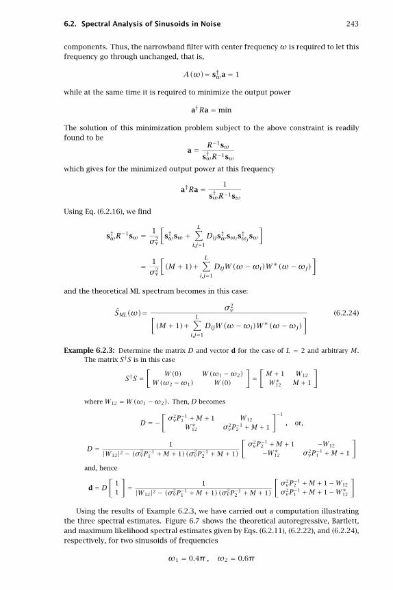
6.2. Spectral Analysis of Sinusoids in Noise 243
components. Thus, the narrowband filter with center frequencyω is required to let thisfrequency go through unchanged, that is,
A(ω)= s†ωa = 1
while at the same time it is required to minimize the output power
a†Ra = min
The solution of this minimization problem subject to the above constraint is readilyfound to be
a = R−1sω
s†ωR−1sω
which gives for the minimized output power at this frequency
a†Ra = 1
s†ωR−1sω
Using Eq. (6.2.16), we find
s†ωR−1sω = 1
σ2v
[s†ωsω +
L∑i,j=1
Dijs†ωsωis†ωjsω
]
= 1
σ2v
[(M + 1)+
L∑i,j=1
DijW(ω−ωi)W∗(ω−ωj)]
and the theoretical ML spectrum becomes in this case:
SML(ω)= σ2v[
(M + 1)+L∑i,j=1
DijW(ω−ωi)W∗(ω−ωj)] (6.2.24)
Example 6.2.3: Determine the matrix D and vector d for the case of L = 2 and arbitrary M.The matrix S†S is in this case
S†S =[
W(0) W(ω1 −ω2)W(ω2 −ω1) W(0)
]=
[M + 1 W12
W∗12 M + 1
]
whereW12 =W(ω1 −ω2). Then, D becomes
D = −[σ2vP−11 +M + 1 W12
W∗12 σ2vP−12 +M + 1
]−1
, or,
D = 1
|W12|2 − (σ2vP−1
1 +M + 1)(σ2vP−1
2 +M + 1)
[σ2vP−12 +M + 1 −W12
−W∗12 σ2vP−11 +M + 1
]
and, hence
d = D[
11
]= 1
|W12|2 − (σ2vP−1
1 +M + 1)(σ2vP−1
2 +M + 1)
[σ2vP−12 +M + 1−W12
σ2vP−11 +M + 1−W∗12
]
Using the results of Example 6.2.3, we have carried out a computation illustratingthe three spectral estimates. Figure 6.7 shows the theoretical autoregressive, Bartlett,and maximum likelihood spectral estimates given by Eqs. (6.2.11), (6.2.22), and (6.2.24),respectively, for two sinusoids of frequencies
ω1 = 0.4π, ω2 = 0.6π

244 6. Spectrum Estimation
and equal powers SNR = 10 log10(P1/σ2v)= 6 dB, and M = 6. To facilitate the com-
parison, all three spectra have been normalized to 0 dB at the frequencyω1 of the firstsinusoid. It is seen that the lengthM = 6 is too short for the Bartlett spectrum to resolvethe two peaks. The AR spectrum is the best (however, close inspection of the graph willreveal a small bias in the frequency of the peaks, arising from the mutual interaction ofthe two sinewaves). The effect of increasing the SNR is shown in Fig. 6.8, where the SNRhas been changed to 12 dB. It is seen that the AR spectral peaks become narrower, thusincreasing their resolvability.
0 0.1 0.2 0.3 0.4 0.5 0.6 0.7 0.8 0.9 1−40
−30
−20
−10
0
digital frequency ω in units of π
dB
M = 6, SNR = 6 dB
ARBartlettML
0 0.1 0.2 0.3 0.4 0.5 0.6 0.7 0.8 0.9 1−40
−30
−20
−10
0
digital frequency ω in units of π
dB
M = 6, SNR = 12 dB
ARBartlettML
Fig. 6.7 and Fig. 6.8 AR, Bartlett, and ML spectrum estimates.
To show the effect of increasingM, we kept SNR = 6 dB, and increased the order toM = 12 and M = 18. The resulting spectra are shown in Figs. 6.9 and 6.10. It is seenthat all spectra tend to become better. The interplay between resolution, order, SNR,and bias has been studied in [18,20,23].
0 0.1 0.2 0.3 0.4 0.5 0.6 0.7 0.8 0.9 1−40
−30
−20
−10
0
digital frequency ω in units of π
dB
M = 12, SNR = 6 dB
ARBartlettML
0 0.1 0.2 0.3 0.4 0.5 0.6 0.7 0.8 0.9 1−40
−30
−20
−10
0
digital frequency ω in units of π
dB
M = 18, SNR = 6 dB
ARBartlettML
Fig. 6.9 and Fig. 6.10 AR, Bartlett, and ML spectrum estimates.
The main motivation behind the definition (6.2.22) for the pseudospectrum was toobtain an expression that exhibits very sharp spectral peaks at the sinusoid frequenciesωi. Infinite resolution can, in principle, be achieved if we can find a polynomial A(z)that has zeros on the unit circle at the desired frequency angles; namely, at
zi = ejωi , i = 1,2, . . . , L (6.2.25)
Pisarenko’s method determines such a polynomial on the basis of the autocorrelationmatrix R. The desired conditions on the polynomial are
A(zi)= A(ωi)= 0 , i = 1,2, . . . , L (6.2.26)

6.2. Spectral Analysis of Sinusoids in Noise 245
where we slightly abuse the notation and write A(ejω)= A(ω). To satisfy these con-ditions, the degree M of the polynomial A(z) must necessarily be M ≥ L; then, theremainingM−L zeros of A(z) could be arbitrary. Let a be the vector of coefficients ofA(z), so that
a =
⎡⎢⎢⎢⎢⎢⎣a0
a1
...aM
⎤⎥⎥⎥⎥⎥⎦ , A(z)= a0 + a1z−1 + · · · + aMz−M
Noting that A(ω)= s†ωa, Eqs. (6.2.26) may be combined into one vectorial equation
S†a =
⎡⎢⎢⎢⎢⎢⎣s†ω1
s†ω2
...
s†ωL
⎤⎥⎥⎥⎥⎥⎦ a =
⎡⎢⎢⎢⎢⎢⎣A(ω1)A(ω2)
...A(ωL)
⎤⎥⎥⎥⎥⎥⎦ = 0 (6.2.27)
But then, Eq. (6.2.9) implies that
Ra = σ2va+ SPS†a = σ2
va
or, that σ2v must be an eigenvalue of R with a the corresponding eigenvector:
Ra = σ2va (6.2.28)
The quantity σ2v is actually the smallest eigenvalue of R. To see this, consider any
other eigenvector a of R, and normalize it to unit norm
Ra = λa , with a†a = 1 (6.2.29)
Then, (6.2.9) implies that
λ = λa†a = a†Ra = σ2va†a+ aSPS†a
= σ2v +
[A(ω1)∗, A(ω2)∗, . . . , A(ωL)∗
]⎡⎢⎢⎢⎢⎢⎣P1
P2
. . .
PL
⎤⎥⎥⎥⎥⎥⎦⎡⎢⎢⎢⎢⎢⎣A(ω1)A(ω2)
...A(ωL)
⎤⎥⎥⎥⎥⎥⎦= σ2
v +L∑i=1
Pi|A(ωi)|2
which shows that λ is equal to σ2v shifted by a non-negative amount. If the eigenvector
satisfies the conditions (6.2.26), then the shift in λ vanishes. Thus, the desired poly-nomial A(z) can be found by solving the eigenvalue problem (6.2.29) and selecting theeigenvector belonging to the minimum eigenvalue. This is Pisarenko’s method [19]. Asa byproduct of the procedure, the noise power levelσ2
v is also determined, which in turnallows the determination of the power matrix P, as follows. Writing Eq. (6.2.9) as
R−σ2vI = SPS†
and acting by S† and S from the left and right, we obtain
P = U†(R−σ2vI)U , where U = S(S†S)−1 (6.2.30)
Since there is freedom in selecting the remaining M − L zeros of the polynomialA(z), it follows that there are (M − L)+1 eigenvectors all belonging to the minimum

246 6. Spectrum Estimation
eigenvalue σ2v . Thus, the (M+1)-dimensional eigenvalue problem (6.2.29) has two sets
of eigenvalues: (a) M + 1 − L degenerate eigenvalues equal to σ2v , and (b) L additional
eigenvalues which are strictly greater than σ2v .
The (M+ 1−L)-dimensional subspace spanned by the degenerate eigenvectors be-longing to σ2
v is called the noise subspace. The L-dimensional subspace spanned bythe eigenvectors belonging to the remaining L eigenvalues is called the signal subspace.Since the signal subspace is orthogonal to the noise subspace. and the L linearly inde-pendent signal vectors sωi , i = 1,2, . . . , L are also orthogonal to the noise subspace, itfollows that the signal subspace is spanned by the sωis.
In the special case when L =M (corresponding to the Pisarenko’s method), there isno degeneracy in the minimum eigenvalue, and there is a unique minimum eigenvector.In this case, allM = L zeros of A(z) lie on the unit circle at the desired anglesωi.
Example 6.2.4: Consider the case L =M = 2. The matrix R is written explicitly as:
R = σ2vI + P1sω1 s†ω1
+ P2sω2 s†ω2, or,
R =⎡⎢⎣ σ2
v + P1 + P2 P1e−jω1 + P2e−jω2 P1e−2jω1 + P2e−2jω2
P1ejω1 + P2ejω2 σ2v + P1 + P2 P1e−jω1 + P2e−jω2
P1e2jω1 + P2e2jω2 P1ejω1 + P2ejω2 σ2v + P1 + P2
⎤⎥⎦It is easily verified that the (unnormalized) vector
a =⎡⎢⎣ a0
a1
a2
⎤⎥⎦ =⎡⎢⎣ 1−(ejω1 + ejω2)ejω1ejω2
⎤⎥⎦is an eigenvector of R belonging to λ = σ2
v . In this case, the polynomial A(z) is
A(z) = a0 + a1z−1 + a2z−2 = 1− (ejω1 + ejω2)z−1 + ejω1ejω2z−2
= (1− ejω1z−1)(1− ejω2z−1)
exhibiting the two desired zeros at the sinusoid frequencies. ��Example 6.2.5: Consider the caseM = 2, L = 1. The matrix R is
R = σ2vI + P1sω1 s†ω1
=⎡⎢⎣ σ2
v + P1 P1e−jω1 P1e−2jω1
P1ejω1 σ2v + P1 P1e−jω1
P1e2jω1 P1ejω1 σ2v + P1
⎤⎥⎦It is easily verified that the three eigenvectors of R are
e0 =⎡⎢⎣ 1−ejω1
0
⎤⎥⎦ , e1 =⎡⎢⎣ 0
1−ejω1
⎤⎥⎦ , e2 =⎡⎢⎣ 1ejω1
e2jω1
⎤⎥⎦belonging to the eigenvalues
λ = σ2v , λ = σ2
v , λ = σ2v + 3P1
The first two eigenvectors span the noise subspace and the third, the signal subspace. Anylinear combination of the noise eigenvectors also belongs to λ = σ2
v . For example, if wetake
a =⎡⎢⎣ a0
a1
a2
⎤⎥⎦ =⎡⎢⎣ 1−ejω1
0
⎤⎥⎦− ρ⎡⎢⎣ 0
1−ejω1
⎤⎥⎦ =⎡⎢⎣ 1−(ρ+ ejω1)ρejω1
⎤⎥⎦the corresponding polynomial is
A(z)= 1− (ρ+ ejω1)z−1 + ρejω1z−2 = (1− ejω1z−1)(1− ρz−1)
showing one desired zero at z1 = ejω1 and a spurious zero. ��

6.2. Spectral Analysis of Sinusoids in Noise 247
The Pisarenko method can also be understood in terms of a minimization criterionof the type (6.2.12), as follows. For any set of coefficients a, define the output signal
en =M∑m=0
amyn−m = a0yn + a1yn−1 + · · · + aMyn−M
Then, the mean output power is expressed as
E = E[e∗nen]= a†Ra = σ2v a†a+
L∑i=1
Pi|A(ωi)|2
Imposing the quadratic constrainta†a = 1 (6.2.31)
we obtain
E = E[e∗nen]= a†Ra = σ2v +
L∑i=1
Pi|A(ωi)|2 (6.2.32)
It is evident that the minimum of this expression is obtained when conditions (6.2.26)are satisfied. Thus, an equivalent formulation of the Pisarenko method is to minimizethe performance index (6.2.32) subject to the quadratic constraint (6.2.31). The ARand the Pisarenko spectrum estimation techniques differ only in the type of constraintimposed on the filter weights a.
We observed earlier that the AR spectral peaks become sharper as the SNR increases.One way to explain this is to note that in the high-SNR limit or, equivalently, in thenoiseless limit σ2
v → 0, the linear prediction filter tends to the Pisarenko filter, whichhas infinite resolution. This can be seen as follows. In the limit σ2
v → 0, the matrix Ddefined in Eq. (6.2.17) tends to
D→ −(S†S)−1
and therefore, R−1 given by Eq. (6.2.16) becomes singular, converging to
R−1 → 1
σ2v
[I − S(S†S)−1S†
]Thus, up to a scale factor the linear prediction solution, R−1u0 will converge to
a = [I − S(S†S)−1S†]u0 (6.2.33)
The matrix [I − S(S†S)−1S†]
is the projection matrix onto the noise subspace, andtherefore, a will lie in that subspace, that is, S†a = 0. In the limit σ2
v → 0, the noisesubspace of R consists of all the eigenvectors with zero eigenvalue, Ra = 0. We notethat the particular noise subspace eigenvector given in Eq. (6.2.33) corresponds to theso-called minimum-norm eigenvector, discussed in Section 6.6.
In his original method, Pisarenko considered the special case when the number ofsinusoids was equal to the filter order, L = M. This implies that the noise subspace isone-dimensional,M+1−L = 1, consisting of a single eigenvector with zero eigenvalue,such that Ra = 0. In this case, the (M + 1)×(M + 1) singular matrix R has rank Mand all its principal submatrices are nonsingular. As we mentioned in Section 5.5, suchsingular Toeplitz matrices admit a general sinusoidal representation. It is obtained bysetting σ2
v = 0 and L =M in Eq. (6.2.8):
R =L∑i=1
Pisωis†ωi , or, R(k)=
L∑i=1
Piejωik

248 6. Spectrum Estimation
In summary, we have discussed the theoretical aspects of four methods of estimatingthe frequencies of sinusoids in noise. In practice, an estimate of the correlation matrixR can be obtained in terms of the sample autocorrelations from a block of data values:
R(k)= 1
N
N−1−k∑n=0
yn+ky∗n , k = 0,1, . . . ,M
The quality of the resulting estimates of the eigenvectors will be discussed in Section6.11 . The AR and Pisarenko methods can also be implemented adaptively. The adaptiveapproach is based on the minimization criteria (6.2.12) and (6.2.32) and will be discussedin Chapter 7, where also some simulations will be presented.
6.3 Superresolution Array Processing
One of the main signal processing functions of sonar, radar, or seismic arrays of sen-sors is to detect the presence of one or more radiating point-sources. This is a problemof spectral analysis, and it is the spatial frequency analog of the problem of extractingsinusoids in noise discussed in the previous section. The same spectral analysis tech-niques can be applied to this problem. All methods aim at producing a high-resolutionestimate of the spatial frequency power spectrum of the signal field incident on the ar-ray of sensors. The directions of point-source emitters can be extracted by identifyingthe sharpest peaks in this spectrum.
In this section, we discuss conventional (Bartlett) beamforming, as well as the max-imum likelihood, linear prediction, and eigenvector based methods, all of which are ofcurrent interest [28–88]. We also discuss some aspects of optimum beamforming forinterference nulling [29–31,103–107].
Consider a linear array ofM + 1 sensors equally spaced at distances d, and a planewave incident on the array at an angle θ1 with respect to the array normal, as shownbelow.
The conventional beamformer introduces appropriate delays at the outputs of eachsensor to compensate for the propagation delays of the wavefront reaching the array.The output of the beamformer (the “beam”) is the sum
e(t)=M∑m=0
ym(t − τm) (6.3.1)
where ym(t), m = 0,1, . . . ,M is the signal at the mth sensor. To reach sensor 1, thewavefront must travel an extra distance d sinθ1, to reach sensor 2 it must travel dis-tance 2d sinθ1, and so on. Thus, it reaches these sensors with a propagation delay ofd sinθ1/c, 2d sinθ1/c, and so on. The last sensor is reached with a delay ofMd sinθ1/cseconds. Thus, to time-align the first and the last sensor, the output of the first sensor

6.3. Superresolution Array Processing 249
must be delayed by τ0 =Md sinθ1/c, and similarly, themth sensor is time-aligned withthe last one, with a delay of
τm = 1
c(M −m)d sinθ1 (6.3.2)
In this case, all terms in the sum (6.3.1) are equal to the value measured at thelast sensor, that is, ym(t − τm)= yM(t), and the output of the beamformer is e(t)=(M + 1)yM(t), thus enhancing the received signal by a factor of M + 1 and hence itspower by a factor (M + 1)2. The concept of beamforming is the same as that of signalaveraging discussed in Example (2.3.5). If there is additive noise present, it will con-tribute incoherently to the output power, that is, by a factor of (M + 1), whereas thesignal power is enhanced by (M + 1)2. Thus, the gain in the signal to noise ratio at theoutput of the array (the array gain) is a factor ofM + 1.
In the frequency domain, the above delay-and-sum operation becomes equivalent tolinear weighting. Fourier transforming Eq. (6.3.1) we have
e(ω)=M∑m=0
ym(ω)e−jωτm
which can be written compactly as:e = aTy (6.3.3)
where a and y are the (M + 1)-vectors of weights and sensor outputs:
a =
⎡⎢⎢⎢⎢⎢⎣e−jωτ0
e−jωτ1
...e−jωτM
⎤⎥⎥⎥⎥⎥⎦ , y =
⎡⎢⎢⎢⎢⎢⎣y0(ω)y1(ω)
...yM(ω)
⎤⎥⎥⎥⎥⎥⎦From now on, we will concentrate on narrow-band arrays operating at a given fre-
quencyω and the dependence onω will not be shown explicitly. This assumes that thesignals from all the sensors have been subjected to narrow-band prefiltering that leavesonly the narrow operating frequency band. The beamformer now acts as a linear com-biner, as shown in Fig. 6.11. A plane wave at the operating frequency ω, of amplitudeA1, and incident at the above angle θ1, will have a value at the space-time point (t, r)given by
A1ejωt−jk·r
Dropping the sinusoidal t-dependence and evaluating this expression on the x-axis,we have
A1e−jkxx
Fig. 6.11 Beamforming

250 6. Spectrum Estimation
where kx is the x-components of the wave vector k
kx = ωc sinθ1
The value of this field at themth sensor, xm =md, is then
A1e−jmk1
where k1 denotes the normalized wavenumber
k1 = kxd = ωdc sinθ1 = 2πdλ
sinθ1 , λ = wavelength (6.3.4)
This is the spatial analog of the digital frequency. To avoid aliasing effects arisingfrom the spatial sampling process, the spatial sampling frequency 1/d must be greaterthan or equal to twice the spatial frequency 1/λ of the wave. Thus, we must haved−1 ≥ 2λ−1, or d ≤ λ/2. Since sinθ1 has magnitude less than one, the samplingcondition forces k1 to lie within the Nyquist interval
−π ≤ k1 ≤ π
In this case the correspondence between k1 and θ1, is unique. For any angle θ andcorresponding normalized wavenumber k, we introduce the phasing, or steering vector
sk =
⎡⎢⎢⎢⎢⎢⎢⎢⎣
1ejk
e2jk
...eMjk
⎤⎥⎥⎥⎥⎥⎥⎥⎦ , k = 2πdλ
sinθ (6.3.5)
In this notation, the plane wave measured at the sensors is represented by the vector
y = A1s∗k1= A1
⎡⎢⎢⎢⎢⎢⎢⎢⎣
1e−jk1
e−2jk1
...e−Mjk1
⎤⎥⎥⎥⎥⎥⎥⎥⎦The steering vector of array weights a, steered towards an arbitrary direction θ, is
also expressed in terms of the phasing vector sk; we have
am = e−jωτm = e−jω(M−m)(d sinθ/c) = e−jMkejmk
or, ignoring the overall common phase e−jMk, we have
a = sk (steering vector towards k = 2πdλ
sinθ) (6.3.6)
The output of the beamformer, steered towards θ, is
e = aTy = sTky = A1 sTk s∗k1= A1 s†k1
sk = A1W(k− k1)∗
where W(·) was defined in Section 6.2. The mean output power of the beamformersteered towards k is
S(k)= E[e∗e]= a†E[y∗yT]a = a†Ra = s†kRsk

6.3. Superresolution Array Processing 251
Using y = A1s∗k1, we find R = E[y∗yT]= P1sk1s†k1
, where P1 = E[|A1|2], and
S(k) = s†kRsk = P1s†ksk1s†k1sk
= P1|W(k− k1)|2
If the beam is steered on target, that is, ifθ = θ1, or, k = k1, then S(k1)= P1(M+1)2
and the output power is enhanced. The response pattern of the array has the same shapeas the function W(k), and therefore its resolution capability is limited to the widthΔk = 2π/(M + 1) of the main lobe of W(k). Setting Δk = (2πd/λ)Δθ, we find thebasic angular resolution to be Δθ = λ/((M+1)d
), or, Δθ = λ/D, whereD = (M+1)d
is the effective aperture of the array. This is the classical Rayleigh limit on the resolvingpower of an optical system with aperture D [28].
Next, we consider the problem of resolving the directions of arrival of multiple planewaves incident on an array in the presence of background noise. We assume L planeswaves incident on an array ofM+1 sensors from angles θi, i = 1,2, . . . , L. The incidentfield is sampled at the sensors giving rise to a series of “snapshots.” At the nth snapshottime instant, the field received at themth sensor has the form [35]
ym(n)= vm(n)+L∑i=1
Ai(n)e−jmki , m = 0,1, . . . ,M (6.3.7)
where Ai(n) is the amplitude of the ith wave (it would be a constant independent oftime if we had exact sinusoidal dependence at the operating frequency), and ki are thenormalized wavenumbers related to the angles of arrival by
ki = 2πdλ
sinθi , i = 1,2, . . . , L (6.3.8)
and vm(n) is the background noise, which is assumed to be spatially incoherent, andalso uncorrelated with the signal amplitudes Ai(n); that is,
E[vm(n)∗vk(n)]= σ2vδmk , E[vm(n)∗Ai(n)]= 0 (6.3.9)
Eq. (6.3.7) can be written in vector form as follows
y(n)= v(n)+L∑i=1
Ai(n)s∗ki (6.3.10)
The autocorrelation matrix of the signal field sensed by the array is
R = E[y(n)∗y(n)T]= σ2vI +
L∑i,j=1
skiPijs†kj (6.3.11)
where I is the (M+1)×(M+1) unit matrix, and Pij is the amplitude correlation matrix
Pij = E[Ai(n)∗Aj(n)] , 1 ≤ i, j ≤ L (6.3.12)
If the sources are uncorrelated with respect to each other, the power matrix Pij isdiagonal. Introducing the (M + 1)×L signal matrix
S = [sk1 , sk2 , . . . , skL]

252 6. Spectrum Estimation
we may write Eq. (6.3.11) asR = σ2
vI + SPS† (6.3.13)
which is the same as Eq. (6.2.9) of the previous section. Therefore, the analytical expres-sions of the various spectral estimators can be transferred to this problem as well. Wesummarize the various spectrum estimators below:
SB(k)= s†kRsk (conventional Bartlett beamformer)
SLP(k)= 1∣∣s†kR−1u0∣∣2 (LP spectrum estimate)
SML(k)= 1
s†kR−1sk(ML spectrum estimate)
For example, for uncorrelated sources Pij = Piδij, the Bartlett spatial spectrum will be
SB(k)= s†kRsk = σ2v(M + 1)+
L∑i=1
Pi|W(k− ki)|2
which gives rise to peaks at the desired wavenumbers ki from which the angles θi canbe extracted. When the beam is steered towards the ith plane wave, the measured powerat the output of the beamformer will be
SB(ki)= σ2v(M + 1)+Pi(M + 1)2+
∑j =iPj|W(ki − kj)|2
Ignoring the third term for the moment, we observe the basic improvement in theSNR offered by beamforming:
Pi(M + 1)2
σ2v(M + 1)
= Piσ2v(M + 1)
If the sources are too close to each other [closer than the beamwidth of W(k)], theresolution ability of the beamformer worsens. In such cases, the alternative spectralestimates offer better resolution, with the LP estimate typically having a better perfor-mance. The resolution capability of both the ML and the LP estimates improves withhigher SNR, whereas that of the conventional beamformer does not.
The Pisarenko method can also be applied here. As discussed in the previous section,the (M+ 1)-dimensional eigenvalue problem Ra = λa has an L-dimensional signal sub-space with eigenvalues greater than σ2
v , and an (M+1−L)-dimensional noise subspacespanned by the degenerate eigenvectors belonging to the minimum eigenvalue of σ2
v .Any vector a in the noise subspace will have at least L zeros at the desired wavenumberfrequencies ki, that is, the polynomial
A(z)= a0 + a1z−1 + a2z−2 + · · · + aMz−M
will have L zeros atzi = ejki , i = 1,2, . . . , L
and (M − L) other spurious zeros. This can be seen as follows: If Ra = σ2va, then
Eq. (6.3.13) implies that
(σ2vI + SPS†)a = σ2
va ⇒ SPS†a = 0
Dotting with a†, we find that a†SPS†a = 0, and since P is assumed to be strictlypositive definite, it follows that S†a = 0, or
S†a =
⎡⎢⎢⎢⎢⎢⎣A(k1)A(k2)
...A(kL)
⎤⎥⎥⎥⎥⎥⎦ = 0

6.3. Superresolution Array Processing 253
The L largest eigenvalues of R correspond to the signal subspace eigenvectors andcan be determined by reducing the original (M + 1)×(M + 1) eigenvalue problem forR into a smaller L×L eigenvalue problem.
Let e be any eigenvector in the signal subspace, that is, Re = λe, with λ > σ2v . It
follows that SPS†e = (λ−σ2v)e. Multiplying both sides by S† we obtain (S†SP)(S†e)=
(λ−σ2v)(S†e), which states that the L-dimensional vector S†e is an eigenvector of the
L×Lmatrix S†SP. We can turn this into a hermitian eigenvalue problem by factoring thepower matrix P into its square root factors, P = GG†, and multiplying both sides of thereduced eigenvalue problem by G†. This gives (G†S†SG)(G†S†e)= (λ−σ2
v)(G†S†e).Thus, we obtain the L×L hermitian eigenvalue problem
F f = (λ−σ2v)f , where F = G†S†SG , f = G†S†e (6.3.14)
The L signal subspace eigenvalues are obtained from the solution of this reducedeigenproblem. From each L-dimensional eigenvector f, one can also construct the cor-responding (M+ 1)-dimensional eigenvector e. Because e lies in the signal subspace, itcan be expressed as a linear combination of the plane waves
e =L∑i=1
ciski = [sk1 , sk2 , . . . , skL]
⎡⎢⎢⎢⎢⎢⎣c1
c2
...cL
⎤⎥⎥⎥⎥⎥⎦ = Sc
It, then, follows from Eq. (6.3.14) that
f = G†S†e = G†S†Sc ⇒ c = (S†S)−1G−†f
and therefore,e = Sc = S(S†S)−1G−†f (6.3.15)
Example 6.3.1: Using the above reduction method, determine the signal subspace eigenvectorsand eigenvalues for the case of two equal-power uncorrelated plane waves and arbitraryM. The 2×2 matrix P becomes proportional to the identity matrix P = P1I. The reducedmatrix F is then
F = P1S†S = P1
[s†1s1 s†1s2
s†2s1 s†2s2
]= P1
[M + 1 W12
W∗12 M + 1
]
where s1 = sk1 , s2 = sk2 , and W12 = W(k1 − k2). In the equal-power case, F is alwaysproportional to S†S, and therefore, f is an eigenvector of that. It follows that (S†S)−1f willbe a scalar multiple of f and that Eq. (6.3.15) can be simplified (up to a scalar factor) toe = Sf. The two eigenvalues and eigenvectors of F are easily found to be
λ−σ2v = P1
(M + 1± |W12|
), f =
[1
±e−jθ12
]
where θ12 is the phase of W12. Using e = Sf, it follows that the two signal subspaceeigenvectors will be
e = s1 ± e−jθ12 s2
The eigenvalue spread of R is in this case
λmax
λmin= σ
2v +
(M + 1+ |W12|
)P1
σ2v
= 1+ SNR · (M + 1+ |W12|)
where SNR = P1/σ2v . It can be written in the form
λmax
λmin= 1+ SNReff ·
(1+ | cosφ12|
)where SNReff = SNR · (M + 1) is the effective SNR of the array, or the array gain, and φ12
is the angle between the two signal vectors, that is, cosφ12 = s†1s2/(‖s1‖ · ‖s2‖
). ��

254 6. Spectrum Estimation
In practice, estimates of the covariance matrix R are used. For example, if the sensoroutputs are recorded over N snapshots, that is, y(n), n = 0,1, . . . ,N − 1, then, thecovariance matrix Rmay be estimated by replacing the ensemble average of Eq. (6.3.11)with the time-average:
R = 1
N
N−1∑n=0
y(n)∗y(n)T (empirical R)
Since the empirical R will not be of the exact theoretical form of Eq. (6.3.11) thedegeneracy of the noise subspace will be lifted somewhat. The degree to which thishappens depends on how much the empirical R differs from the theoretical R. Onecan still use the minimum eigenvector a to define the polynomial A(z) and from it anapproximate Pisarenko spectral estimator
SP(k)= 1
|A(z)|2 , where z = ejk
which will have sharp and possibly biased peaks at the desired wavenumber frequencies.
Example 6.3.2: Consider the case L =M = 1, defined by the theoretical autocorrelation matrix
R = σ2vI + P1sk1 s†k1
=[σ2v + P1 P1e−jk1
P1ejk1 σ2v + P1
]
Its eigenvectors are:
e0 =[
1−ejk1
], e1 = sk1 =
[1ejk1
]
belonging to the eigenvalues λ0 = σ2v and λ1 = σ2
v + 2P1, respectively. Selecting as thearray vector
a = e0 =[
1−ejk1
]
we obtain a polynomial with a zero at the desired location:
A(z)= a0 + a1z−1 = 1− ejk1z−1
Now, suppose that the analysis is based on an empirical autocorrelation matrix R whichdiffers from the theoretical one by a small amount:
R = R+ΔR
Using standard first-order perturbation theory, we find the correction to the minimumeigenvalue λ0 and eigenvector e0
λ0 = λ0 +Δλ0 , e0 = e0 +Δc e1
where the first-order correction terms are
Δλ0 = e†0(ΔR)e0
e†0e0
, Δc = e†1(ΔR)e0
(λ0 − λ1)e†1e1
The change induced in the zero of the eigenpolynomial is found as follows
a = e0 =[
1−ejk1
]+Δc
[1ejk1
]=
[1+Δc
−(1−Δc)ejk1
]
so thatA(z)= (1+Δc)−(1−Δc)ejk1z−1

6.3. Superresolution Array Processing 255
and the zero is now at
z1 = 1−Δc1+Δc e
jk1 � (1− 2Δc)ejk1
to first-order in Δc. Since Δc is generally complex, the factor (1− 2Δc) will cause both achange (bias) in the phase of the zero ejk1 , and will move it off the unit circle reducing theresolution. Another way to see this is to compute the value of the polynomial steered ontarget; that is,
A(k1)= s†k1a = s†k1
(e0 +Δc e1)= Δc s†k1e1 = 2Δc
which is small but not zero. ��
The high resolution properties of the Pisarenko and other eigenvector methods de-pend directly on the assumption that the background noise field is spatially incoherent,resulting in the special structure of the autocorrelation matrix R. When the noise isspatially coherent, a different eigenanalysis must be carried out. Suppose that the co-variance matrix of the noise field v is
E[v∗vT]= σ2vQ
where Q reflects the spatial coherence of v. Then the covariance matrix of Eq. (6.3.13)is replaced by
R = σ2vQ + SPS† (6.3.16)
The relevant eigenvalue problem is now the generalized eigenvalue problem
Ra = λQa (6.3.17)
Consider any such generalized eigenvector a, and assume it is normalized such that
a†Qa = 1 (6.3.18)
Then, the corresponding eigenvalue is expressed as
λ = λa†Qa = a†Ra = σ2va†Qa+ a†SPS†a = σ2
v + a†SPS†a
which shows that the minimum eigenvalue is σ2v and is attained whenever a†SPS†a = 0,
or equivalently (assuming that P has full rank), S†a = 0, or, A(ki)= 0, i = 1,2, . . . , L.Therefore, the eigenpolynomial A(z) can be used to determine the wavenumbers ki.
Thus, the procedure is to solve the generalized eigenvalue problem and select theminimum eigenvector. This eigenvalue problem is also equivalent to the minimizationproblem
E = a†Ra = min , subject to a†Qa = 1 (6.3.19)
This criterion, and its solution as the minimum eigenvector, is equivalent to theunconstrained minimization of the Rayleigh quotient, that is,
a†Ra
a†Qa= min � Ra = λminQa (6.3.20)
The practical implementation of the method requires knowledge of the noise covari-ance matrix Q, which is not always possible to obtain. Covariance difference methods[71–74] can be used in the case of unknown Q. Such methods work with measurementsfrom two different arrays, translated or rotated with respect to each other. Assumingthat the background noise is invariant under translation or rotation, the covariance ma-trices of the two arrays will be R1 = S1P1S
†1 + σ2
vQ and R2 = S2P2S†2 + σ2
vQ. Theeigenstructure of the covariance difference R1 −R2 = S1P1S
†1 − S2P2S
†2 can be used to
extract the signal information.

256 6. Spectrum Estimation
The two spectral analysis problems discussed in this and the previous section—direction finding and harmonic retrieval—are dual to each other; one dealing with spatialfrequencies and the other with time frequencies. The optimum processing part is thesame in both cases. The optimum processor does not care how its inputs are supplied, itonly “sees” the correlations among the inputs and its function is to “break down” thesecorrelations thereby extracting the sinusoidal components. The two cases differ only inthe way the inputs to the optimum processor are supplied. This conceptual separationbetween the input part and the optimum processing part is shown in Fig. 6.12. In thetime series case, the correlations among the inputs are sequential correlations in time,whereas in the array case they are spatial correlations, such as those that exist along acoherent wavefront.
Fig. 6.12 Duality between time series and array problems.
A problem related, but not identical, to direction finding is that of optimum beam-forming for interference nulling [29–31,103–107]. In this case, one of the plane waves,say, sk1 , is assumed to be a desired plane wave with known direction of arrival θ1, orwavenumber k1. The other plane waves are considered as interferers or jammers tobe nulled. Assuming for simplicity uncorrelated sources, the covariance matrix (6.3.11)may be decomposed into a part due to the desired signal and a part due to the noiseplus interference:
R = σ2vI +
L∑i=1
Pi sis†i = P1s1s†1 +
[σ2vI +
L∑i=2
Pi sis†i
]= P1s1s†1 +Rn
where we denoted si = ski . The output power of the array with weights a will be
E = a†Ra = P1|s†1a|2 + a†Rna (6.3.21)
The first term is the output power due to the desired signal; the second term isdue to the presence of noise plus interference. This expression suggests two possibleoptimization criteria for a. First, choose a to maximize the relative signal to noise plus

6.3. Superresolution Array Processing 257
interference ratio (SNIR):
SNIR = P1|s†1a|2a†Rna
= max (6.3.22)
The second criterion is to keep the output of the array toward the look direction s1
fixed, while minimizing the output power:
s†1a = 1 and E = a†Ra = P1 + a†Rna = min (6.3.23)
This is equivalent to minimizing the noise plus interference term a†Rna. These twocriteria are essentially equivalent. This is seen as follows. Equation (6.3.22) is equivalentto minimizing the inverse function SNIR−1. Adding one to it, we obtain the equivalentcriterion
1+ SNIR−1 = 1+ a†Rna
P1|s†1a|2 =a†Ra
P1|s†1a|2 = min
This is identical to the Rayleigh quotient (6.3.20) with the choice Q = P1s1s†1. It isequivalent to the minimum eigenvector solution of
Ra = λQa = λP1s1s†1a = μs1 ⇒ a = μR−1s1
where we put all the scalar factors into μ. Similarly, the constraint s†1a = 1 impliesthat a†Q1a = 1 with Q1 = s1s†1. It follows from Eq. (6.3.19), applied with Q1, that thesolution of Eq. (6.3.23) is again the generalized eigenvector
Ra = λ1Q1a = λ1s1s†1a = μ1s1 ⇒ a = μ1R−1s1
Thus, up to a scale factor, the optimum solution for both criteria is
a = R−1s1 (6.3.24)
This solution admits, yet, a third interpretation as the Wiener solution of an ordinarymean-square estimation problem. The term y1(n)= A1(n)s∗1 of Eq. (6.3.10) is the de-sired signal. A reference signal x(n) could be chosen to correlate highly with this termand not at all with the other terms in Eq. (6.3.10). For example, x(n)= f(n)A1(n). Thearray weights can be designed by demanding that the scalar output of the array, aTy(n),be the best mean-square estimate of x(n). This gives the criterion
E[|x(n)−aTy(n)|2] = E[|x(n)|2]− a†r− r†a+ a†Ra
where we set r = E[x(n)y(n)∗]. Minimizing with respect to a (and a∗) gives the Wienersolution a = R−1r. Now, because x(n) is correlated only with y1(n), it follows that rwill be proportional to s1:
r = E[x(n)y(n)∗]= E[x(n)y1(n)∗]= E[x(n)A1(n)∗] s1
Thus, again up to a scale, we obtain the solution (6.3.24). Using the matrix inversionlemma (see Problem 6.6), we can write the inverse of R = P1s1s†1 +Rn, in the form
R−1 = R−1n − cR−1
n s1s†1R−1n , c = (P−1
1 + s†1R−1n s1)−1
Acting by both sides on s1, we find
R−1s1 = c1R−1n s1 , c1 = cP−1
1

258 6. Spectrum Estimation
Therefore, the optimal solution can also be written (up to another scale factor) interms of the noise plus interference covariance matrix Rn:
a = R−1n s1 (6.3.25)
These solutions, known as steered solutions, are sometimes modified to include arbi-trary tapering weights for the array—replacing the steering vector s1 with a generalizedsteering vector
s =
⎡⎢⎢⎢⎢⎢⎣b0
b1ejk1
...bMejk1M
⎤⎥⎥⎥⎥⎥⎦ = B s1 , B = diag{b0, b1, . . . , bM} (6.3.26)
The weightsbm can be chosen to attain a prescribed shape for the quiescent responseof the array in absence of interference. Typical choices are (with k1 = 0)
s =
⎡⎢⎢⎢⎢⎢⎣10...0
⎤⎥⎥⎥⎥⎥⎦ , s =
⎡⎢⎢⎢⎢⎢⎣11...1
⎤⎥⎥⎥⎥⎥⎦To appreciate the properties of the optimum solution, we consider the case of one
jammer, so thatR = P1s1s†1 +Rn , Rn = σ2
vI + P2s2s†2
Using the matrix inversion lemma on R−1n , we obtain
R−1n =
1
σ2v
[I − 1
σ2vP−1
2 + s†2s2
s2s†2
]
Therefore, the optimum solution given by Eq. (6.3.25) becomes
a = R−1n s1 = 1
σ2v
[s1 − P2W(k2 − k1)
σ2v + P2(M + 1)
s2
]
where we used s†2s2 = M + 1 and s†2s1 = W(k2 − k1). Dropping the overall factor of1/σ2
v , we find for the array pattern as a function of wavenumber k or angle θ
A(k)= s†ka =W(k− k1)− P2W(k2 − k1)σ2v + P2(M + 1)
W(k− k2) (6.3.27)
In the absence of the jammer, P2 = 0, we obtain the usual quiescent Bartlett response,W(k− k1). The presence of the second term, called a retrodirective beam, will partiallydistort the quiescent pattern but it will suppress the jammer. Indeed, the array responsesteered toward the jammer at k = k2, becomes
A(k2)=W(k2 − k1)− P2W(k2 − k1)σ2v + P2(M + 1)
W(0)= W(k2 − k1)σ2v + P2(M + 1)
The ratio A(k2)/W(k2 − k1) is the array response, in the direction of the jammer,relative to the quiescent response. Thus, if the signal to noise ratio SNR2 = P2/σ2
v islarge, the jammer will be suppressed. Only in the limit of infinite SNR is the jammercompletely nulled.
The reason for the incomplete nulling can be traced, as in the case of linear predic-tion, to the linear constraint on the weights (6.3.23). To get exact nulling of the jammers,

6.4. Eigenvector Methods 259
we must force the zeros of the polynomial a to lie on the unit circle at the jammer posi-tions. As suggested by Problem 6.13, this can be accomplished by imposing a quadraticconstraint a†Qa = const., where Q must be chosen as Q = σ2
vI + P1s1s†1 instead ofQ = P1s1s†1. The optimum weight is the minimum eigenvector solution of the general-ized eigenproblem Ra = λQa and will have exact zeros at the jammer positions. As inthe linear prediction case, the linearly constrained optimum beamformer solution tendsto this eigenvector solution in the limit σ2
v → 0.
6.4 Eigenvector Methods
The single most important property of eigenvector methods is that, at least in principle,they produce unbiased frequency estimates with infinite resolution, regardless of thesignal to noise ratios. This property is not shared by the older methods. For example,the resolution of the Bartlett method is limited by the array aperture, and the resolutionof the linear prediction and maximum likelihood methods degenerates with decreasingSNRs. Because of this property, eigenvector methods have received considerable atten-tion in signal processing and have been applied to several problems, such as harmonicretrieval, direction finding, echo resolution, and pole identification [19,45–99]. In theremainder of this chapter, we discuss the theoretical aspects of eigenvector methods infurther detail, and present several versions of such methods, such as MUSIC, Minimum-Norm, and ESPRIT.
We have seen that the eigenspace of the covariance matrixR consists of two mutuallyorthogonal parts: the (M+1−L)-dimensional noise subspace spanned by the eigenvec-tors belonging to the minimum eigenvalue σ2
v , and the L-dimensional signal subspacespanned by the remaining L eigenvectors having eigenvalues strictly greater than σ2
v .Let ei, i = 0,1, . . . ,M, denote the orthonormal eigenvectors of R in order of increasingeigenvalue, and let K = M + 1 − L denote the dimension of the noise subspace. Then,the first K eigenvectors, ei, i = 0,1, . . . , K − 1, form an orthonormal basis for the noisesubspace, and the last L eigenvectors, ei, i = K,K+1, . . . ,M, form a basis for the signalsubspace. We arrange these basis vectors into the eigenvector matrices:
EN = [e0, e1, . . . , eK−1], ES = [eK, eK+1, . . . , eM] (6.4.1)
Their dimensions are (M + 1)×K and (M + 1)×L. The full eigenvector matrix of R is:
E = [EN, ES]= [e0, e1, . . . , eK−1, eK, eK+1, . . . , eM] (6.4.2)
The orthonormality of the eigenvectors is expressed by the unitarity property E†E =I, where I is the (M+1)-dimensional unit matrix. The unitarity can be written in termsof the submatrices (6.4.1):
E†NEN = IK , E†NES = 0 , E†SES = IL (6.4.3)
where IK and IL are the K×K and L×L unit matrices. The completeness of the eigenvec-tors is expressed also by the unitarity of E, i.e., EE† = I. In terms of the submatrices, itreads:
ENE†N + ESE†S = I (6.4.4)
These two terms are the projection matrices onto the noise and signal subspaces.We have seen that the L signal direction vectors ski belong to the signal subspace, andtherefore, are expressible as linear combinations of ES. It follows that the signal matrixS = [sk1 , . . . , skL] is a non-orthogonal basis of the signal subspace and must be relatedto ES by S = ESC, where C is an L×L invertible matrix. Using the orthonormality of ES,

260 6. Spectrum Estimation
it follows that S†S = C†E†SESC = C†C. Thus, the projector onto the signal subspacemay be written as
PS = ESE†S = (SC−1)(C−†S†)= S(C†C)−1S† = S(S†S)−1S† (6.4.5)
We may also obtain a non-orthogonal, but useful, basis for the noise subspace. Wehave seen that an (M+1)-dimensional vector e lies in the noise subspace—equivalently,it is an eigenvector belonging to the minimum eigenvalue σ2
v—if and only if the corre-sponding order-M eigenfilter E(z) has L zeros on the unit circle at the desired signalzeros, zi = ejki , i = 1,2, . . . , L, and has M − L = K − 1 other spurious zeros. Such apolynomial will factor into the product:
E(z)= A(z)F(z)= A(z)[f0 + f1z−1 + · · · + fK−1z−(K−1)] (6.4.6)
where the zeros of F(z) are the spurious zeros, and A(z) is the reduced-order polyno-mial of order L whose zeros are the desired zeros; that is,
A(z)=L∏i=1
(1− ejkiz−1)= 1+ a1z−1 + · · · + aLz−L (6.4.7)
Introducing the K delayed polynomials:
Bi(z)= z−iA(z) , i = 0,1, . . . , K − 1 (6.4.8)
we may write Eq. (6.4.6) in the form
E(z)= f0B0(z)+f1B1(z)+· · · + fK−1BK−1(z)=K−1∑i=0
fiBi(z) (6.4.9)
and in coefficient form
e =K−1∑i=0
fi bi = [b0, b1, . . . , bK−1]
⎡⎢⎢⎢⎢⎢⎣f0f1...fK−1
⎤⎥⎥⎥⎥⎥⎦ ≡ B f (6.4.10)
Because each of the polynomials Bi(z) has L desired zeros, it follows that the cor-responding vectors bi will lie in the noise subspace. Thus, the matrix B defined inEq. (6.4.10) will be a non-orthogonal basis of the noise subspace. It is a useful ba-sis because the expansion coefficients f of any noise subspace vector e are the coef-ficients of the spurious polynomial F(z) in the factorization (6.4.6). Put differently,Eq. (6.4.10) parametrizes explicitly the spurious degrees of freedom arising from theK-fold degeneracy of the minimum eigenvalue. The basis vectors bi, considered as(M + 1)-dimensional vectors, are simply the delayed versions of the vector of coeffi-cients, a = [1, a1, . . . , aL]T, of the polynomial A(z), that is,
bi =[0, . . . , 0︸ ︷︷ ︸i zeros
, 1, a1, . . . , aL, 0, . . . , 0︸ ︷︷ ︸K−1−i zeros
]T(6.4.11)
For example, in the case L = 2 andM = 5, we have K =M + 1− L = 4 and B is:
B = [b0, b1, b2, b3]=
⎡⎢⎢⎢⎢⎢⎢⎢⎢⎣
1 0 0 0a1 1 0 0a2 a1 1 00 a2 a1 10 0 a2 a1
0 0 0 a2
⎤⎥⎥⎥⎥⎥⎥⎥⎥⎦

6.5. MUSIC method 261
It follows that the basis B must be linearly related to the orthonormal basis EN byB = ENC, where C is a K×K invertible matrix. Then, B†B = C†C and the projector ontothe noise subspace becomes:
PN = ENE†N = (BC−1)(C−†B†)= B(C†C)−1B† = B(B†B)−1B† (6.4.12)
Combining Eqs. (6.4.12) and (6.4.5), we may write the completeness relation (6.4.4)in terms of the non-orthogonal bases B and S:
B(B†B)−1B† + S(S†S)−1S† = I (6.4.13)
The objective of all eigenvector methods is to estimate the signal zeros zi = ejki ,i = 1,2, . . . , L. All methods begin with an eigenanalysis of R, such that EN and ES areavailable. In practice, the eigenanalysis is based on the sample covariance matrix Rdefined on the basis of a finite number of snapshots, say N:
R = 1
N
N−1∑n=0
y(n)∗y(n)T (6.4.14)
Sometimes, a symmetrized version is preferred, obtained from R by
Rs = 1
2(R+ JR∗J) (6.4.15)
where J the (M+1)-dimensional reversing matrix. The matrix Rs is invariant under re-versal, that is, JRsJ = R∗s . This version is appropriate when the theoreticalR is Toeplitz.This case arises if and only if the L×L power matrix P is diagonal; that is, when the Lsources are mutually uncorrelated. As the number of snapshots increases, the eigen-structure of R or Rs becomes a better and better approximation of the eigenstructureof R. Such asymptotic statistical properties will be discussed in Section 6.11. Next, wediscuss several practical approaches.
6.5 MUSIC method
Let Ei(z) denote the eigenfilters of the noise subspace eigenvectors ei, i = 0,1, . . . , K−1.According to Eq. (6.4.5), we can write Ei(z)= A(z)Fi(z), which shows that Ei(z) havea common set of L zeros at the desired signal locations, but each may have a differentset of K − 1 spurious zeros. It is possible for these spurious zeros to lie very closeto or on the unit circle. Therefore, if only one eigenfilter is used, there may be anambiguity in distinguishing the desired zeros from the spurious ones. The multiplesignal classification (MUSIC) method [46,48] attempts to average out the effect of thespurious zeros by forming the sum of the magnitude responses of the K noise subspaceeigenfilters, that is, setting z = ejk,
1
K
K−1∑i=0
|Ei(k)|2 = |A(k)|2 1
K
K−1∑i=0
|Fi(k)|2
Because the polynomials Fi(z) are all different, the averaging operation will tend tosmear out any spurious zero of any individual term in the sum. Thus, the above expres-sion will effectively vanish only at the L desired zeros of the common factor|A(k)|2.The MUSIC pseudospectrum is defined as the inverse
SMUS(k)= 1
1
K
K−1∑i=0
|Ei(k)|2(6.5.1)

262 6. Spectrum Estimation
It will exhibit peaks at the L desired wavenumbers ki, i = 0,1, . . . , L. The sum mayalso be replaced by a weighted sum [54]. The sum may be written compactly in termsof the projection matrices onto the noise or signal subspaces. Noting that |Ei(k)|2 =s†k(eie
†i )sk, we find
K−1∑i=0
|Ei(k)|2 = s†k
⎡⎣K−1∑i=0
eie†i
⎤⎦ sk = s†kENE†Nsk = s†k(I − ESE†S)sk
where we used Eq. (6.4.4). The practical version of the MUSIC method is summarizedbelow:
1. Based on a finite number of snapshots, compute the sample covariance matrixR, solve its eigenproblem, and obtain the estimated eigenvector matrix E witheigenvalues arranged in increasing order.
2. Estimate the dimension K of the noise subspace as the number of the smallest,approximately equal, eigenvalues. This can be done systematically using the AICor MDL criteria discussed later. The estimated number of plane waves will beL =M + 1−K. Divide E into its noise and signal subspace parts, EN and ES.
3. Compute the spectrum (6.5.1) and extract the desired wavenumbers ki from theL peaks in this spectrum.
The Akaike (AIC) and minimum description length (MDL) information-theoretic cri-teria have been suggested to determine the number of plane waves that are present, orequivalently, the dimension of the noise subspace [61]. They are defined by
AIC(k) = −2NkL(k)+2(M + 1− k)(M + 1+ k)
MDL(k) = −NkL(k)+1
2(M + 1− k)(M + 1+ k)log(N)
(6.5.2)
for k = 1,2, . . . ,M + 1, where N is the number of snapshots and L(k) is a likelihoodfunction defined as the log of the ratio of the harmonic and arithmetic means of thefirst k estimated eigenvalues {λ0, λ1, . . . , λk−1} of R; namely,
L(k)= ln
⎡⎢⎢⎣ (λ0λ1 · · · λk−1)1/k
1
k(λ0 + λ1 + · · · + λk−1)
⎤⎥⎥⎦The dimension K of the noise subspace is chosen to be that k that minimizes the
functions AIC(k) or MDL(k). The above definition is equivalent to that of [61], butproduces the value of K instead of L. The routine aicmdl (see Appendix B) takes asinputs the M + 1 estimated eigenvalues in increasing order and the number N, andcomputes the values of the AIC and MDL functions. Once K is known, an estimate ofthe minimum eigenvalue can be obtained by
σ2v = λmin = 1
K(λ0 + λ1 + · · · + λK−1) (6.5.3)
Next, we present some simulation examples. First, we compare the MUSIC methodagainst the linear prediction method. We considered two uncorrelated equal-powerplane waves incident on an array of 8 sensors (M = 7). The SNR of the waves, de-fined by SNRi = 10 log10(Pi/σ2
v), was −5 dB and their wavenumbers k1 = 0.2π andk2 = 0.4π. For half-wavelength array spacing (d = λ/2), these correspond, through(6.3.8), to the angles of arrival θ1 = 11.54o and θ2 = 23.58o.
The number of snapshots was N = 500. The snapshots were simulated usingEq. (6.3.10). Each v(n) was generated as a complex vector of M + 1 zero-mean in-dependent gaussian components of variance σ2
v = 1.

6.5. MUSIC method 263
Note that to generate a zero-mean complex random variable v of variance σ2v , one
must generate two zero-mean independent real random variables v1 and v2, each withvariance σ2
v/2 and set v = v1 + jv2; then, E[v∗v]= E[v21]+E[v2
2]= 2(σ2v/2)= σ2
v .The amplitudes Ai(n) were assumed to have only random phases; that is, Ai(n)=(Pi)1/2ejφin , whereφin, were independent angles uniformly distributed in [0,2π]. Theroutine snap (see Appendix B) takes as input an integer seed, generates a snapshot vec-tor y, and updates the seed. Successive calls to snap, in conjunction with the (complexversion) of the routine sampcov, can be used to generate the sample covariance matrixR. In this particular example, we used the symmetrized version Rs, because the twosources were uncorrelated.
Figure 6.13 shows the MUSIC spectrum computed using Eq. (6.5.1) together with theLP spectrum SLP(k)= 1/|s†ka|2, where a = R−1
s u0. Because each term in the sum (6.5.1)arises from a unit-norm eigenvector, we have normalized the LP vector a also to unitnorm for the purpose of plotting the two spectra on the same graph. Increasing thenumber of snapshots will improve the MUSIC spectrum because the covariance matrixRs will become a better estimate of R, but it will not improve the LP spectrum becausethe theoretical LP spectrum does not perform well at low SNRs.
0 0.2 0.4 0.6 0.8 1−10
0
10
20
30
40
wavenumber k in units of π
dB
MUSIC and LP spectra
MUSICLP
Fig. 6.13 MUSIC and LP spectra.
To facilitate the computation and manipulation of spectra, we have included thefollowing small routines. The routine norm converts a vector a to a unit-norm vector.The routine fresp computes the magnitude response squared, |A(k)|2 = |s†ka|2, of anMth order filter a at a specified number of equally-spaced frequency points within theright-half of the Nyquist interval, 0 ≤ k ≤ π. It can be modified easily to include the en-tire Nyquist interval or any subinterval. The routine invresp inverts a given spectrum,S(k)→ 1/S(k). The routines abs2db and db2abs convert a spectrum from absoluteunits to decibels and back, S(k)= 10 log10 S(k). The routine select picks out any eigen-vector from the M + 1 ones of the eigenvector matrix E. The routine music computesEq. (6.5.1) over a specified number of frequency points. It is built out of the routinesselect, fresp, and invresp.
In the second simulation example, we increased the SNR of the two plane waves to10 dB and reduced the number of snapshots to N = 100. The theoretical and empiricaleigenvalues of R and Rs, were found to be
i 0 1 2 3 4 5 6 7
λi 1 1 1 1 1 1 61.98 100.02
λi 0.70 0.76 0.83 0.87 1.05 1.28 64.08 101.89

264 6. Spectrum Estimation
The values of the AIC and MDL functions were
k 1 2 3 4 5 6 7 8
AIC(k) 126.0 120.3 111.4 98.7 87.2 81.1 2544.2 3278.2MDL(k) 145.1 138.3 127.4 111.9 94.4 77.0 1291.6 1639.1
0 0.2 0.4 0.6 0.8 1−10
0
10
20
30
40
50
60
70
80
wavenumber k in units of π
dBNoise eigenvector spectra
e0
e1
e2
Fig. 6.14 Spectra of the first three noise subspace eigenvectors.
Both functions achieve their minimum value at K = 6 and therefore, L = M + 1 −K = 2. The estimated value of σ2
v , computed by Eq. (6.5.3), was σ2v = 0.915. Figure
6.14 shows the spectra of the first three noise subspace eigenvectors; namely, Si(k)=1/|Ei(k)|2 = 1/|s†kei|2, for i = 0,1,2. We note the presence of a common set of peaksat the two desired wavenumbers and several spurious peaks. The spurious peaks aredifferent, however, in each spectrum and therefore, the averaging operation will tendto eliminate them. The averaged MUSIC spectrum, based on all K = 6 noise subspaceeigenvectors, is plotted in Figure 6.15 using the same scale as in Fig. 6.14.
The averaging operation has had two effects. First, the removal of all spurious peaksand second, the broadening and reduction in sharpness of the two desired peaks. Thisbroadening is the result of statistical sampling; that is, using R instead ofR, causes smallbiases in the peaks of individual eigenvectors about their true locations. These biasesare not inherent in the theoretical method, as they are in the linear prediction case; theyare statistical in nature and disappear in the limit of large number of snapshots. Figure6.15 also shows the performance of the minimum-norm method, which we discuss next.It appears to produce somewhat sharper peaks than MUSIC, but it can sometimes exhibithigher levels of spurious peaks.
6.6 Minimum-Norm Method
The minimum-norm method [47,53] attempts to eliminate the effect of spurious zerosby pushing them inside the unit circle, leaving the L desired zeros on the circle. Thisis accomplished by finding a noise subspace vector d = [d0, d1, . . . , dM]T such that thecorresponding eigenfilter D(z) will have all its spurious zeros within the unit circle.This means that in the factorization (6.4.6), D(z)= A(z)F(z), the spurious polynomialF(z) must be chosen to have all its zeros strictly inside the unit circle, equivalently,F(z) must be a minimum-phase polynomial. If F(z) were the prediction-error filter ofa linear prediction problem, then it would necessarily be a minimum-phase filter. Thus,the design strategy for d is to make F(z) a linear prediction filter. This can be done byrequiring that d have minimum norm subject to the constraint that its first coefficient

6.6. Minimum-Norm Method 265
be unity; that is,d†d = min , subject to u†0d = d0 = 1 (6.6.1)
The minimization is carried over the noise subspace vectors. In the B basis (6.4.10),the vector d is expressed by d = B f, where f are the coefficients of F(z), and theconstraint equation becomes u†0B f = 1. With the exception of b0, all basis vectors bistart with zero; therefore, u†0B = [u†0b0,u
†0b1, . . . ,u
†0bK−1]= [1,0, . . . ,0]≡ u†, that is, a
K-dimensional unit vector. Therefore, in the B basis Eq. (6.6.1) becomes
d†d = f†Raa f = min , subject to u†f = 1 (6.6.2)
where we set Raa = B†B. This is recognized as the Toeplitz matrix of autocorrelationsof the filter a, as defined in Section 3.3. For the 6×4 example above, we verify
Raa = B†B =
⎡⎢⎢⎢⎣Raa(0) Raa(1)∗ Raa(2)∗ 0Raa(1) Raa(0) Raa(1)∗ Raa(2)∗
Raa(2) Raa(1) Raa(0) Raa(1)∗
0 Raa(2) Raa(1) Raa(0)
⎤⎥⎥⎥⎦where Raa(0)= |a0|2 + |a1|2 + |a2|2, Raa(1)= a1a∗0 + a2a∗1 , Raa(2)= a2a∗0 , andRaa(3)= 0. Note that the autocorrelation function of an order-M filter a vanishes forlags greater than M + 1. It follows that Eq. (6.6.2) represents an ordinary linear predic-tion problem and its solution f will be a minimum-phase filter with all its zeros insidethe unit circle. Up to a scale factor, we may write this solution as f = R−1
aau = (B†B)−1u.Writing u = B†u0, we have f = (B†B)−1B†u0, and the solution for d becomes
d = B f = B(B†B)−1B†u0 = ENE†Nu0 (6.6.3)
This is the solution of criterion (6.6.1) up to a scale. Interestingly, the locations ofthe spurious zeros do not depend on the signal to noise ratios, but depend only on thedesired zeros on the unit circle. This follows from the fact that the solution for f dependsonly on B. Using Eq. (6.4.13), we may also write d in terms of the signal subspace basis
d = [I − ESE†S
]u0 =
[I − S(S†S)−1S†
]u0
Recall from Section 6.2 that this is the large-SNR limit of the LP solution. Noting thatE†Nu0, is the complex conjugate of the top row of the eigenvector matrix EN, we writeEq. (6.6.3) explicitly as a linear combination of noise subspace eigenvectors
d =K−1∑i=0
E∗0iei (6.6.4)
where E∗0i the conjugate of the 0i-th matrix element of E. The subroutine minorm com-putes d using Eq. (6.6.4). The corresponding pseudospectrum estimate is defined as theinverse magnitude response of the filter d
SMIN(k)= 1
|D(k)|2 =1
|s†kd|2(6.6.5)
The practical implementation of this method requires the same two initial steps asMUSIC; namely, eigenanalysis of R and estimation of K. In Fig. 6.15, the minimum-normspectrum was computed by calling the routines minorm. The vector d was normalized tounit norm to make a fair comparison with the MUSIC spectrum. Looking at the spectra isnot the best way to evaluate this method because the spurious zeros—even though insidethe unit circle—interact with the desired zeros to modify the shape of the spectrum.The minimum-norm method is better judged by comparing the theoretical and empirical

266 6. Spectrum Estimation
zeros of the polynomialD(z), computed fromR and R. They are shown in the followingtable. The first two zeros are the desired ones.
zeros of D(z)theoretical empirical
|zi| arg(zi)/π |zi| arg(zi)/π1.0000 0.2000 0.9989 0.20201.0000 0.4000 1.0059 0.40260.8162 −0.1465 0.8193 −0.14410.7810 −0.4251 0.7820 −0.42270.7713 −0.7000 0.7759 −0.69840.8162 0.7465 0.8188 0.74810.7810 −0.9749 0.7832 −0.9729
0 0.2 0.4 0.6 0.8 1−10
0
10
20
30
40
50
60
70
80
wavenumber k in units of π
dB
MUSIC and min− norm spectra
min− normmusic
Fig. 6.15 MUSIC and min-norm spectra.
The main idea of the minimum-norm method was to separate the desired zeros fromthe spurious ones by pushing the latter inside the unit circle. In some applications ofeigenvector methods, such as pole identification, the desired zeros lie themselves insidethe unit circle (being the poles of a stable and causal system) and therefore, cannot beseparated from the spurious ones. To separate them, we need a modification of themethod that places all the spurious zeros to the outside of the unit circle. This can bedone by replacing the vector f by its reverse fR = J f∗, where J is the K×K reversingmatrix. The resulting polynomial will be the reverse of F(z), with all its zeros reflectedto the outside of the unit circle. The reverse vector fR is the backward prediction filterobtained by minimizing (6.6.2) subject to the constraint that its last element be unity.Using the reversal invariance of Raa, namely, JRaaJ = R∗aa, we find
fR = J f∗ = J(R−1aa)∗u = R−1
aaJu = R−1aav
where v = Ju = [0, . . . ,0,1]T is the reverse of u. With the exception of bK−1, the lastelement of all basis vectors bi is zero. Denoting by v0, the reverse of u0, it follows thatv†0B = [0,0, . . . ,0, aL]= aLv†. Thus, up to a scale factor, v can be replaced by B†v0,and hence, The vector d becomes
d = B fR = B(B†B)−1B†v0 = ENE†Nv0 (6.6.6)
Up to a scale, this is the minimum-norm vector subject to the constraint that itslast element be unity; that is, v†0d = dM = 1. In terms of the matrix elements of theeigenvector matrix E it reads
d =K−1∑i=0
E∗Miei (6.6.7)

6.7. Reduced-Order Method 267
where E∗Mi is the conjugate of the last row of E. The spurious zeros of this vector willlie outside the unit circle. We may refer to this method as the modified minimum-normmethod.
6.7 Reduced-Order Method
The basis B of the noise subspace has very special structure, being constructed in termsof the delayed replicas of the same reduced-order vector a. It is evident from Eq. (6.4.11)that a can be extracted from any column bi or B by advancing it by i units. The B basisis linearly related to the orthonormal eigenvector basis by B = ENC with some K×Kinvertible matrix C. Thus, the vector bi is expressible as a linear combination of thenoise subspace eigenvectors
bi =K−1∑j=0
ejCji , i = 0,1, . . . , K − 1
This vector has a total of K−1 vanishing coefficients, namely, the first i and the lastK−1− i coefficients. Component-wise, we may write bim = 0, for 0 ≤m ≤ i−1 and fori+ L+ 1 ≤ m ≤ M. This vector may be specified up to an overall scale factor becausewe are interested only in the zeros of the reduced-order vector a. Therefore, we mayarbitrarily fix one of the coefficients Cji to unity. For example, we may single out the0th eigenvector:
bi = e0 +K−1∑j=1
ejCji (6.7.1)
If e0 happens to be absent from the sum, we may single out e1 and so on. Thecoefficient bii will no longer be unity, but may be normalized so later. TheK−1 unknowncoefficients Cji, j = 1,2, . . . , K − 1 can be determined by the K − 1 conditions that thefirst i and lastK−1−i coefficients of bi be zero. Written in terms of the matrix elementsof the eigenvector matrix E, these conditions read for each i = 0,1, . . . , K − 1:
Em0 +K−1∑j=1
EmjCji = 0 , for 0 ≤m ≤ i− 1 and i+ L+ 1 ≤m ≤M (6.7.2)
Thus, solving the linear Eqs. (6.7.2) for the coefficients Cji and substituting in Eq.(6.7.1), we obtain bi and, advancing it by i units, the reduced-order vector a. BecauseBi(z)= z−iA(z), the polynomial Bi(z) has no spurious zeros. In effect, forming thelinear combination Eq. (6.7.1) of noise subspace eigenvectors removes the spurious zeroscompletely by placing them at the origin of the z-plane. In a sense, this procedure carriesthe philosophy of the minimum-norm method further.
When the theoretical R is replaced by the empirical R and the corresponding EN isreplaced by the estimated EN, it is no longer possible to linearly transform the basisEN to a B basis constructed from a single reduced-order vector a. It is still possible,however, to form linear combinations of the estimated eigenvectors.
bi =K−1∑j=0
ejCji , i = 0,1, . . . , K − 1 (6.7.3)
such that the resulting vectors bi will have vanishing first i and lastK−1−i coefficients;that is, of the form
bi =[0, . . . , 0︸ ︷︷ ︸i zeros
, 1, ai1, . . . , aiL, 0, . . . , 0︸ ︷︷ ︸K−1−i zeros
]T(6.7.4)

268 6. Spectrum Estimation
This can be done by solving Eq. (6.7.2) with E replaced by its estimate, E, obtainedfrom R. The resultingK reduced-order vectors ai = [1, ai1, . . . , aiL]T, i = 0,1, . . . , K−1,will not be the same necessarily. But, each can be considered to be an approximateestimate of the true reduced-order vector a, and its L zeros will be estimates of the truedesired zeros.
It turns out that individually none of the ai is a particularly good estimate of a. Theymay be combined, however, to produce a better estimate. This is analogous to MUSIC,where individual spectra of noise eigenvectors are not good, but combining them byaveraging produces a better spectrum. To see how we may best combine the ai, weform a new basis of the estimated noise subspace in terms of the vectors bi, namely,B = [b0, b1, . . . , bK−1]. For our 6×4 example, we have
B = [b0, b1, b2, b3]=
⎡⎢⎢⎢⎢⎢⎢⎢⎢⎣
1 0 0a01 1 0 0a02 a11 1 00 a12 a21 10 0 a22 a31
0 0 0 a32
⎤⎥⎥⎥⎥⎥⎥⎥⎥⎦The linear transformations (6.7.3) may be written compactly as B = ENC. Note that
B†B is no longer Toeplitz and therefore, the LP solution f of (6.6.2) will not necessarilyhave minimum phase. Thus, the empirical minimum-norm solution can have spuriouszeros outside or near the unit circle. Because the basis B is an estimate of the true B,we may try to fit B to a matrix of the type B having the special structure (6.4.11) byminimizing the distance between the two matrices according to some matrix norm. Forexample, we may minimize the Frobenius matrix distance [102]:
‖B− B‖2 = tr[(B− B)†(B− B)] = K−1∑
i=0
‖bi − bi‖2 = min
Because bi and bi are the delayed versions of the reduced-order vectors ai and a , itfollows that ‖bi − bi‖2 = ‖ai − a‖2. Therefore,
‖B− B‖2 = tr[(B− B)†(B− B)] = K−1∑
i=0
‖ai − a‖2 = min (6.7.5)
Minimizing with respect to a gives the result:
a = 1
K
K−1∑i=0
ai , A(z)= 1
K
K−1∑i=0
Ai(z) (6.7.6)
that is, the average of the K filters. Thus, we obtain the following reduced-order or,reduced-MUSIC algorithm [75]:
1. Solve the eigenproblem for the estimated covariance matrix R.
2. Using the estimated noise subspace eigenvectors, solve (6.7.2) for the coefficientsCji and using Eq. (6.7.3) obtain the basis vectors bi and hence the reduced-ordervectors ai, i = 0,1, . . . , K − 1.
3. Use the average (6.7.6) to get an estimate A(z) of the reduced-order polynomialA(z). Obtain estimates of the desired zeros by a root-finding procedure on A(z),or, by finding the peaks in the pseudospectrum
S(k)= 1
|A(k)|2 =1
|s†ka|2(6.7.7)
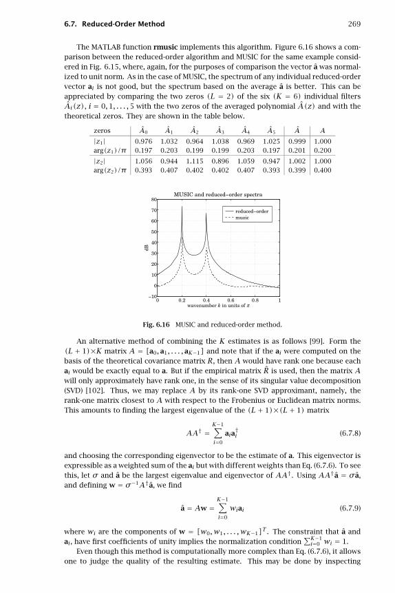
6.7. Reduced-Order Method 269
The MATLAB function rmusic implements this algorithm. Figure 6.16 shows a com-parison between the reduced-order algorithm and MUSIC for the same example consid-ered in Fig. 6.15, where, again, for the purposes of comparison the vector a was normal-ized to unit norm. As in the case of MUSIC, the spectrum of any individual reduced-ordervector ai is not good, but the spectrum based on the average a is better. This can beappreciated by comparing the two zeros (L = 2) of the six (K = 6) individual filtersAi(z), i = 0,1, . . . ,5 with the two zeros of the averaged polynomial A(z) and with thetheoretical zeros. They are shown in the table below.
zeros A0 A1 A2 A3 A4 A5 A A|z1| 0.976 1.032 0.964 1.038 0.969 1.025 0.999 1.000arg(z1)/π 0.197 0.203 0.199 0.199 0.203 0.197 0.201 0.200
|z2| 1.056 0.944 1.115 0.896 1.059 0.947 1.002 1.000arg(z2)/π 0.393 0.407 0.402 0.402 0.407 0.393 0.399 0.400
0 0.2 0.4 0.6 0.8 1−10
0
10
20
30
40
50
60
70
80
wavenumber k in units of π
dB
MUSIC and reduced− order spectra
reduced− ordermusic
Fig. 6.16 MUSIC and reduced-order method.
An alternative method of combining the K estimates is as follows [99]. Form the(L+ 1)×K matrix A = [a0, a1, . . . , aK−1] and note that if the ai were computed on thebasis of the theoretical covariance matrix R, then A would have rank one because eachai would be exactly equal to a. But if the empirical matrix R is used, then the matrix Awill only approximately have rank one, in the sense of its singular value decomposition(SVD) [102]. Thus, we may replace A by its rank-one SVD approximant, namely, therank-one matrix closest to A with respect to the Frobenius or Euclidean matrix norms.This amounts to finding the largest eigenvalue of the (L+ 1)×(L+ 1) matrix
AA† =K−1∑i=0
aia†i (6.7.8)
and choosing the corresponding eigenvector to be the estimate of a. This eigenvector isexpressible as a weighted sum of the ai but with different weights than Eq. (6.7.6). To seethis, let σ and a be the largest eigenvalue and eigenvector of AA†. Using AA†a = σa,and defining w = σ−1A†a, we find
a = Aw =K−1∑i=0
wiai (6.7.9)
where wi are the components of w = [w0,w1, . . . ,wK−1]T. The constraint that a andai, have first coefficients of unity implies the normalization condition
∑K−1i=0 wi = 1.
Even though this method is computationally more complex than Eq. (6.7.6), it allowsone to judge the quality of the resulting estimate. This may be done by inspecting

270 6. Spectrum Estimation
the relative magnitudes of the singular values of A, equivalently, the L+ 1 eigenvaluesof AA†. Theoretically, all but the maximum eigenvalue must be zero. Applying thismethod to the above simulation example, we find the estimated zeros:
z1 = 0.9985ej0.2011π , z2 = 1.0037ej0.3990π
and the theoretical and empirical SVD values of the matrix A:
theoretical 5.8059 0 0empirical 5.8139 0.1045 0.0187
6.8 Maximum Likelihood Method
The maximum likelihood method is not, strictly speaking, an eigenvector method; how-ever, some of the ideas we have been discussing apply to it. The method determines theplane wave frequencies and amplitudes by fitting them directly to the measured snap-shot data using a criterion, such as maximum likelihood or least-squares [76–79]. Eachsnapshot is modeled according to Eq. (6.3.10), which can be written compactly as
y(n)= [s∗k1, . . . , s∗kL
]⎡⎢⎢⎣A1(n)
...AL(n)
⎤⎥⎥⎦+ v(n)= S∗A(n)+v(n) (6.8.1)
The unknown amplitudes A(n) and wavenumbers ki, i = 1,2, . . . , L are treated asdeterministic parameters to be fitted to the snapshot data Y = {y(n), 0 ≤ n ≤ N − 1}.The maximum likelihood estimates of these parameters are obtained by maximizing thejoint density of the snapshots, p(Y)= max. If the wave parameters are deterministic,then the randomness in y(n) arises only from v(n). Assuming that v(n) are complexgaussian (see Problem 6.16) and independent, the joint density of Y is the product ofmarginal densities:
p(Y) =N−1∏n=0
p(v(n)
) = 1
(πσ2v)N(M+1) exp
⎡⎣− 1
σ2v
N−1∑n=0
‖v(n)‖2
⎤⎦= 1
(πσ2v)N(M+1) exp
⎡⎣− 1
σ2v
N−1∑n=0
‖y(n)−S∗A(n)‖2
⎤⎦Thus, under gaussian statistics, the maximum likelihood criterion is equivalent to
the least-squares minimization criterion:
J =N−1∑n=0
‖y(n)−S∗A(n)‖2 = min (6.8.2)
According to the general discussion of [101], the simultaneous minimization of Jwith respect to ki and A(n) can be done in two steps. First, minimize with respect tothe amplitudes A(n) and then, minimize with respect to the wavenumbers ki. Settingthe gradients with respect to A(n) to zero, we obtain
∂J∂A(n)
= −S†[y(n)∗−SA∗(n)] = 0 ⇒ A(n)∗= (S†S)−1S†y(n)∗
Inserting this solution into Eq. (6.8.2), we obtain
J =N−1∑n=0
‖y(n∗)−SA(n)∗‖2 =N−1∑n=0
∥∥[I − S(S†S)−1S†]y(n)∗∥∥2

6.9. ESPRIT Method 271
Using Eq. (6.4.13), we may rewrite it in terms of the projector onto the noise subspace,namely, PN = B(B†B)−1B† = I − S(S†S)−1S†
J =N−1∑n=0
∥∥B(B†B)−1B†y(n)∗∥∥2 =
N−1∑n=0
∥∥PNy(n)∗∥∥2
Using the projection property P†NPN = PN, and the definition (6.4.14) of the samplecovariance matrix, we find
J =N−1∑n=0
y(n)TPNy(n)∗= tr
⎡⎣N−1∑n=0
PNy(n)Ty(n)∗⎤⎦ = N tr[PNR]
The minimization of J with respect to the coefficients of the reduced-order vector ais a highly nonlinear problem. It may be solved, however, iteratively by the solution of asuccession of simpler problems, by the following procedure [91,77–79,95,97]. Writey(n)TB = [y(n)Tb0,y(n)Tb1, . . . ,y(n)TbK−1] and note that y(n)Tbi = aTyi(n),where yi(n) is the (L + 1)-dimensional portion of y(n) starting at the ith position,namely,
yi(n)=[yi(n), yi+1(n), . . . , yi+L(n)
]T , i = 0,1, . . . , K − 1
Then, y(n)TB = aT[y0(n),y1(n), . . . ,yK−1(n)]≡ aTY(n). And, J can be written as
J =N−1∑n=0
y(n)TB(B†B)−1B†y(n)∗= aT
⎡⎣N−1∑n=0
Y(n)(B†B)−1Y(n)†⎤⎦ a∗
The minimization of J is obtained by solving the succession of problems, for i = 1,2, . . . ,
Ji = aTi
⎡⎣N−1∑n=0
Y(n)(B†i−1Bi−1)−1Y(n)†⎤⎦ a∗i = min (6.8.3)
where B†i−1Bi−1 is constructed from the solution ai−1 of the previous iteration. Theiteration is initialized by a0 = [1,0, . . . ,0]T, which gives B†0B0 = IK. At each iteration,Eq. (6.8.3) is subject to an appropriate constraint on ai such as that its first coefficientbe unity, or, that its zeros lie on the unit circle. Note that B†B is Toeplitz and therefore,its inverse can be computed efficiently by the Levinson recursion.
6.9 ESPRIT Method
There exist a number of eigenvector methods that employ two or more sets of snap-shot measurements obtained from two or more arrays related to each other either bytranslation or by rotation. Examples are the estimation of signal parameters via rota-tional invariance techniques (ESPRIT) method [80–82], the covariance difference method[71–74], and the spatial smoothing method for dealing with coherent signals [55,62].
Consider two arrays related to each other by an overall translation by distance Δalong the x-axis. The effect of translation shows up as an overall phase change in eachdirection vector. For example, the value of a wave on the x-axis with respect to theoriginal and the translated x-axes will be:
A1e−jkxx → A1e−jkx(x+Δ) = A1e−jkxxe−jkxΔ
Setting xm = md and letting δ = Δ/d be the displacement in units of d, we obtainat the original and translatedmth array elements
A1e−jk1m → A1e−jk1me−jk1δ

272 6. Spectrum Estimation
or, in terms of the direction vectors
A1s∗1 → A1s∗1 e−jk1δ
It follows that the matrix S = [sk1 , . . . , skL] transforms under translation as
S → SDδ , Dd = diag{ejk1δ, ejk2δ, . . . , ejkLδ
}(6.9.1)
Therefore, the snapshot measurements at the original and translated arrays are
y(n) = S∗A(n)+v(n)
yδ(n) = S∗D∗δA(n)+vδ(n)(6.9.2)
The covariance and cross-covariance matrices are
Ryy = E[y(n)∗y(n)T]= SPS† +σ2vI
Ryδyδ = E[yδ(n)∗yδ(n)T]= SDδPD†δS† +σ2vI
(6.9.3)
Ryyδ = E[y(n)∗yδ(n)T]= SPD†δS† (6.9.4)
where we used E[vδ(n)∗vδ(n)T]= E[v(n)∗v(n)T]= σ2vI and E[v(n)∗vδ(n)T]= 0.
The ESPRIT method works with the matrix pencil, C(λ)= C − λCδ, defined by thepair of matrices
C = Ryy −σ2vI = SPS† , Cδ = Ryyδ = SPD†δS† (6.9.5)
The generalized eigenvalues of this matrix pencil are, by definition [102], the so-lutions of det(C − λCδ)= 0, and the corresponding generalized eigenvectors satisfyCe = λCδe. The ESPRIT method is based on the observation that the nonzero general-ized eigenvalues of C(λ) are simply
λi = ejkiδ , i = 1,2, . . . , L (6.9.6)
and therefore, the desired wavenumbers ki can be extracted from the knowledge of theλi. Note that λ = 0 is a generalized eigenvalue because det(C)= det(SPS†)= 0. Thisfollows from the fact that SPS† is an (M + 1)×(M + 1) matrix of rank L < M + 1.The generalized eigenvectors corresponding to λ = 0 are the vectors in the null spaceof SPS†; namely, they satisfy SPS†e = 0, or, equivalently, S†e = 0. These are thenoise subspace eigenvectors of Ryy. Next, we show that the only nonzero generalizedeigenvalues are those in Eq. (6.9.6). The corresponding generalized eigenvector e mustsatisfy
SPS†e = λSPD†δS†eMultiplying both sides by S† and removing the common matrix factor (S†S)P, we
obtain S†e = λD†δS†e. Using the fact that D†δ = D−1δ , and defining the L-dimensional
vector f = S†e, we obtainDδf = λf
Clearly, if e is not in the noise subspace, then f = S†e = 0; therefore, λ must be aneigenvalue ofDδ, which is already diagonal. This proves Eq. (6.9.6). The eigenvectors ofDδ will be the L-dimensional unit vectors; that is, the columns of the L×L unit matrix,fi = ui, i = 1,2, . . . , L. The generalized eigenvectors will be ei = S(S†S)−1ui. Theseare obtained by an argument similar to Eq. (6.3.15). Thus, the L columns of the ma-trix S(S†S)−1 are simply the generalized eigenvectors corresponding to the generalizedeigenvalues (6.9.6).

6.10. Spatial Smoothing 273
In the practical implementation of the method, we assume we have two sets of snap-shots, y(n) and yδ(n), for n = 0,1, . . . ,N− 1, measured at the original and translatedarrays. The covariance matrix Ryy is estimated by Eq. (6.4.14) and the cross-covariancematrix by
Cδ = Ryyδ =1
N
N−1∑n=0
y(n)∗yδ(n)T
From the eigenproblem of Ryy, we obtain an estimate of σ2v , either as the mini-
mum eigenvalue or, as the average of the eigenvalues of the noise subspace. Then, setC = Ryy − σ2
vI and solve the generalized eigenproblem for the pair {C, Cδ}. The Lgeneralized eigenvalues closest to the unit circle are used to extract estimates of thedesired wavenumbers ki by Eq. (6.9.6).
Unlike the minimum-norm and reduced-order methods that require equally spacedlinear arrays, the MUSIC and ESPRIT methods can be applied to arrays of arbitrary ge-ometry.
6.10 Spatial Smoothing
Eigenvector methods rely on the property that the noise subspace eigenvectors have atleast L zeros on the unit circle at the desired frequency locations. As we saw in Section6.3, this property requires that the L×L power matrix P have full rank equal to L. Torepeat the argument, the condition Ra = σ2
va implies that SPS†a = 0, but what we wantis S†a = 0. Multiplying by a†, we obtain (S†a)†P(S†a)= 0, but this does not necessarilyimply that S†a = 0 unless P has full rank.
The case of diagonal P corresponds to mutually uncorrelated sources for the L planewaves. The case of a nondiagonal P of full rank implies that the sources are partiallycorrelated. The case of a non-diagonal P with less than full rank implies that some orall of the sources are coherent with each other. This case commonly arises in multipathsituations, as shown in the following diagram
To see how eigenvector methods fail if P does not have full rank, consider the worstcase when all the sources are coherent, which means that the wave amplitudes Ai(n)are all proportional to each other, say, Ai(n)= ciA1(n), i = 1,2, . . . , L, where the ci = 0(with c1 = 1) are attenuation factors corresponding to the different paths. Compactly,we may write A(n)= A1(n)c. Then, the power matrix becomes
P = E[A(n)∗A(n)T
] = E[|A1(n)|2]c∗cT = P1c∗cT (6.10.1)
It has rank one. The corresponding covariance matrix is
R = SPS† +σ2vI = P1Sc∗cTS† +σ2
vI = P1ss† +σ2vI (6.10.2)
where s = Sc∗. Similarly,
y(n)= A1(n)S∗c+ v(n)= A1(n)s∗ + v(n)
Because R is a rank-one modification of the identity matrix, it will have a one-dimensional signal subspace spanned by s and a noise subspace of dimension K =

274 6. Spectrum Estimation
M + 1− 1 = M spanned by the eigenvectors belonging to the minimum eigenvalue σ2v .
Thus, although we have L different signals, the solution of the eigenproblem will resultin a one-dimensional signal subspace. Moreover, the noise eigenvectors, will not neces-sarily have zeros at the L desired locations. This can be seen as follows. If Ra = σ2
va,then P1ss†a = 0, or, s†a = cTS†a = 0, which gives
cTS†a = [c1, . . . , cL]
⎡⎢⎢⎣A(k1)
...A(kL)
⎤⎥⎥⎦ = L∑i=1
ciA(ki)= 0
This does not imply that the individual terms in the sum are zero. One solution tothis problem is the method of spatial smoothing [55,62], which restores P to full rank,so that the eigenstructure methods can be applied as usual. The method is as follows.The given array of M + 1 sensors is subdivided into J subarrays each having M + 1sensors. The first subarray consists of the first M+ 1 elements of the given array. Eachsubsequent subarray is obtained by shifting ahead one array element at a time, as shownin the following diagram
Formally, we define the J subarrays by
yi(n)= [yi(n), yi+1(n), . . . , yi+M(n)]T , i = 0,1, . . . , J − 1 (6.10.3)
where the bar indicates that the size of the subarray is M + 1. That is the (M + 1)-dimensional portion of y(n) starting at the ith array element. Using Eq. (6.9.2), we maywrite compactly
yi(n)= S∗D∗i A(n)+vi(n)
where S is the same as S but of dimension M + 1. The matrix Di is given by Eq. (6.9.1)with δ = i, corresponding to translation by i units. The covariance matrix of the ithsubarray will be
Ri = E[yi(n)∗yi(n)T]= SDiPD†i S† +σ2vI
where I is the (M+1)-dimensional identity matrix. The average of the subarray covari-ances is
R = 1
J
J−1∑i=0
Ri = SPS† +σ2vI (6.10.4)
where
P = 1
J
J−1∑i=0
DiPD†i (6.10.5)
To be able to resolve L sources by the (M + 1)-dimensional eigenproblem (6.10.4),we must have M ≥ L, and the rank of P must be L. It has been shown [62] that if thenumber of subarrays J is greater than the number of signals, J ≥ L, then, P has fullrank. If the J subarrays are to fit within the original array of lengthM+1, then we musthave M + 1 ≥ (M + 1)+(J − 1), that is, the length of the first subarray plus the J − 1subsequent shifts. Thus, M + 1 ≥ M + J. If both J and M are greater than L, then wemust haveM + 1 ≥ 2L. Therefore, the price for restoring the rank of P is that we mustuse twice as long an array as in the ordinary full-rank case with L sources. A somewhat

6.10. Spatial Smoothing 275
stronger result is that J ≥ L+1−ρ, where ρ is the rank of P [86]; equivalently, we haveJ ≥ ν+1, where ν = L−ρ is the nullity of P. This would give for the minimum numberof array elementsM + 1 ≥ 2L+ 1− ρ [63,79,86].
Following [62], we derive the condition J ≥ L for the worst case, when all the signalsare coherent. In that case, P has rank one (ρ = 1) and is given by Eq. (6.10.1); P becomes
P = P1
J
J−1∑i=0
Dic∗cTD†i =P1
J
J−1∑i=0
did†i , di = Dic∗
Writing∑J−1i=0 did
†i = DD†, where D = [d0,d1, . . . ,dJ−1], it follows that the rank of
P is the same as the rank of D. The matrix element Dli is the lth component of the ithcolumn; that is, Dli = (di)l= c∗l ejkli. Thus, D can be written as the product, D = C∗V,of the diagonal matrix C∗ = diag{c∗1 , . . . , c∗L } and the L×J Vandermonde matrix V withmatrix elements Vli = ejkli; for example, if L = 3 and J = 4,
V =⎡⎢⎣ 1 ejk1 e2jk1 e3jk1
1 ejk2 e2jk2 e3jk2
1 ejk3 e2jk3 e3jk3
⎤⎥⎦The rank of Vandermonde matrices is always full; that is, it is the minimum of the col-
umn and row dimensions, min(L, J). It follows that the rank of P is equal to min(L, J),therefore, it is equal to L only if J ≥ L.
To appreciate the mechanism by which the rank is restored, let us consider an ex-ample with two (L = 2) fully coherent sources. The minimum number of subarraysneeded to decohere the sources is J = L = 2. This implies M =M+ 1− J =M− 1. Thecovariance matrix of the full array is
R = P1[s1, s2][c∗1c∗2
][c1, c2]
[s†1s†2
]+σ2
vI
The covariance matrices of the two subarrays are
R0 = P1[s1, s2][c∗1c∗2
][c1, c2]
[s†1s†2
]+σ2
vI
R1 = P1[s1, s2][ejk1c∗1ejk2c∗2
][e−jk1c1, e−jk2c2]
[s†1s†2
]+σ2
vI
Their average becomes
R = 1
2(R0 + R1)= [s1, s2]P
[s†1s†2
]+σ2
vI
where
P = P1
2
[c∗1c∗2
][c1, c2]+P1
2
[ejk1c∗1ejk2c∗2
][e−jk1c1, e−jk2c2]
= P1
[c∗1 c1 c∗1 c2
(1+ ej(k1−k2)
)/2
c1c∗2(1+ ej(k2−k1)
)/2 c∗2 c2
]Clearly, P is non-singular. The presence of the translation phases makes the two
column vectors [c∗1 , c∗2 ]T and [ejk1c∗1 , ejk2c∗2 ]T linearly independent. The determinantof P is easily found to be
det P = |c1c2|2 sin2(k1 − k2
2
)

276 6. Spectrum Estimation
Perhaps, an even simpler example is to consider the two quadratic forms
Q0 = (f1 + f2)2= fT[
11
][1,1]f , f =
[f1f2
]
Q1 = f21 = fT
[10
][1,0]f
Separately, they have rank one, but their sum has full rank
Q = Q0 +Q1 = (f1 + f2)2+f21 = 2f2
1 + 2f1f2 + f22 = fT
[2 11 1
]f
where the 2×2 coefficient matrix has rank two, being the sum of two rank-one matricesdefined by two linearly independent two-dimensional vectors[
2 11 1
]=
[11
][1,1]+
[10
][1,0]
Such quadratic forms can be formed, for example, by a†SPS†a = f†Pf, where f = S†a.In the practical implementation of the method, the subarray covariances are computedby sample averages over N snapshots; that is,
Ri = 1
N
N−1∑n=0
yi(n)∗yi(n)T
and then forming the average
R = 1
J
J−1∑i=0
Ri
In addition to spatial smoothing, there exist other methods for dealing with theproblem of coherent signal sources [83,84,87,88].
6.11 Asymptotic Properties
Statistically, the sample covariance matrix R approximates the theoretical R, and there-fore, the linear predictor based on R will approximate the one based on R. Similarly, theeigenstructure of R will approximate that of R. In this section, we derive the asymptoticstatistical properties that justify such approximations [108–142].
The basic technique for deriving asymptotic results is to perform a linearization ofthe empirical solution about the theoretical one and then use the asymptotic statisticalproperties of R. In Section 1.5, we obtained the asymptotic covariance of R for a largenumber of snapshots N:
E[ΔRijΔRkl]= 1
N(RikRjl +RilRjk) (6.11.1)
where ΔR = R−R is the deviation of R from its mean. This was valid in the real-valuedcase; the complex-valued version will be considered shortly. The normal equations oflinear prediction based on R and R are
Ra = Eu0 , a =[
1ααα
]and Ra = Eu0 , a =
[1ααα
]
where E and E are the minimized values of the mean-square prediction errors given byE = aTRa and E = aTRa. Setting a = a+Δa and E = E +ΔE, we obtain
(R+ΔR)(a+Δa)= (E +ΔE)u0 ⇒ R(Δa)+(ΔR)a = (ΔE)u0 (6.11.2)

6.11. Asymptotic Properties 277
where we kept only the first-order terms. Because a and a have first coefficient of unity,Δa = a− a will have zero first coefficient, that is, uT0 (Δa)= 0. Multiplying both sides ofEq. (6.11.2) by aT, we obtain aTR(Δa)+aT(ΔR)a = ΔE. Using the normal equations fora, we have aTR(Δa)= EuT0 (Δa)= 0. Thus, ΔE = aT(ΔR)a. Solving Eq. (6.11.2) for Δaand using R−1u0 = E−1a, we find
Δa = E−1(ΔE)a−R−1(ΔR)a , ΔE = aT(ΔR)a (6.11.3)
For the purpose of computing the asymptotic covariances of Δa and ΔE, it provesconvenient to express Eq. (6.11.3) in terms of the vector δa ≡ (ΔR)a. Then,
Δa = E−1(ΔE)a−R−1(δa) , ΔE = aT(δa) (6.11.4)
Using Eq. (6.11.1), we find for the covariance of δa
E[δaiδak] = E[∑jΔRijaj
∑lΔRklal
] =∑jlE[ΔRijΔRkl]ajal
= 1
N
∑jl(RikRjl +RjkRil)ajal = 1
N[Rik(aTRa)+(Ra)i(aTR)k
]or,
E[δaδaT]= 1
N[ER+Ra aTR] (6.11.5)
Writing ΔE = δaTa, we find
E[δaΔE]= E[δaδaT]a = 1
N[ER+Ra aTR]a = 1
N[ERa+Ra(aTRa)
] = 2ENRa
Using this result, we find for the asymptotic variance of E:
E[(ΔE)2] = aTE[δaΔE]= 2E
NaTRa = 2E2
N(6.11.6)
This generalizes Eq. (1.15.2). Similarly, we find for the cross-covariance between Eand a:
E[ΔaΔE]= E[(E−1ΔEa−R−1δa)ΔE
] = E−1E[(ΔE)2]a−R−1E[δaΔE] , or,
E[ΔaΔE]= E−1 2E2
Na−R−1(2E
NRa
) = 0 (6.11.7)
Finally, we find for the covariance of the predictor a
E[ΔaΔaT]= E[Δa(E−1ΔEaT − δaR−1)
] = −E[ΔaδaT]R−1
= −E[(E−1aΔE −R−1δa)δaT
]R−1 = −[
E−1a2EN
aTR−R−1 1
N(ER+Ra aTR)
]R−1
= EN(R−1 − E−1a aT)= E
N
[0 0T
0 R−1
]
where we used Eq. (5.9.16) or (1.7.35), and R is the lower-order portion of R. Such result
was expected because Δa is of the form Δa =[
0Δααα
]. Thus,
E[ΔαααΔαααT]= ENR−1 (6.11.8)

278 6. Spectrum Estimation
This is a well-known result, and although we obtained it for sample covariance ma-trices of the type (1.5.21), where the snapshots y(n) were assumed to be independent,it can be proved in the case of autoregressive models where R is built out of the sampleautocorrelation function [108,118–121,125–128,133].
It can also be shown that asymptotically E and ααα are the maximum likelihood esti-mates of the LP parameters E and ααα, having all the good properties of such estimates,namely, asymptotic unbiasedness, consistency, efficiency, and gaussian distributionabout the theoretical values with covariances given by Eqs. (6.11.6)–(6.11.8), which arenone other than the Cramer-Rao bounds of these parameters. It is instructive to use thegeneral formula (1.17.17) to derive these bounds, where the parameter vector is definedas λλλ = [E,αααT]T. We must determine the dependence of R on these parameters andthen compute the derivatives ∂R/∂E and ∂R/∂ααα. We write the UL factorization of R inthe form of Eq. (1.7.33):
R =[ρa rTara R
]= U−1DaU−T =
[1 αααT
0 U
]−1 [E 0T
0 D
][1 0T
ααα UT
]
The parametrization ofR on the parameters E andααα is shown explicitly. It is evidentthat the entries ρa and ra depend on E andααα, whereas R does not. We have
ra = −Rααα , ρa = E −αααTra = E +αααTRααα
Working with differentials, we find dra = −Rdααα and dρa = dE + 2αααTRdααα. Differ-entiating R entry-by-entry and using Eq. (1.7.35) for R−1, we find
R−1dR = E−1
[dE +αααTRdααα −dαααTR
(dE +αααTRdααα)ααα− Edααα −αααdαααTR]
(6.11.9)
Writing a similar expression for a second differential R−1δR, multiplying the two,and taking the trace, we find
tr(R−1dRR−1δR)= E−2dEδE + 2E−1dαααTRδααα (6.11.10)
This gives for the matrix elements of the Fisher information matrix
JEE = 1
2N tr
[R−1∂R
∂ER−1∂R
∂E
]= N
2E2
JαE = 1
2N tr
[R−1 ∂R
∂αααR−1∂R
∂E
]= 0
Jαα = 1
2N tr
[R−1 ∂R
∂αααR−1 ∂R
∂αααT
]= NER
As we know, the inverse of the information matrix is the Cramer-Rao bound forunbiased estimates. This inverse agrees with Eqs. (6.11.6)–(6.11.8).
Following the discussion of [123,129], we may also derive the asymptotic covariancesof the reflection coefficients. The forward and backward Levinson recursion establishesa one-to-one correspondence between the prediction coefficients ααα and the vector ofreflection coefficientsγγγ. Therefore, we have the differential correspondenceΔγγγ = ΓΔααα,where Γ is the matrix of partial derivatives Γij = ∂γi/∂αj. It follows that the asymptoticcovariance of γγγ will be
E[ΔγγγΔγγγT]= ΓE[ΔαααΔαααT]ΓT = ENΓR−1ΓT (6.11.11)

6.11. Asymptotic Properties 279
Example 6.11.1: For the first-order case, we have R = [R(0)] and E1 = (1 − γ21)R(0), where
γ1 = −a11. Thus, we obtain Eq. (1.15.2) as a special case
E[(Δa11)2
] = E[(Δγ1)2
] = 1− γ21
N
For the second-order case, Δααα = [Δa12, Δa22]T , and we have E2 = R(0)(1−γ21)(1−γ2
2)and R is the order-one autocorrelation matrix. Thus, we find
E[ΔαααΔαααT] = E2
NR−1 = E2
N
[R(0) R(1)R(1) R(0)
]−1
= (1− γ21)(1− γ2
2)N(1− γ2
1)
[1 −γ1
−γ1 1
]= 1− γ2
2
N
[1 −γ1
−γ1 1
]
From the Levinson recursion, we find for the second-order predictor a22 = −γ1(1 − γ2)and a22 = −γ2. Differentiating, we have
dααα =[da12
da22
]=
[−(1− γ2) γ1
0 −1
][dγ1
dγ2
]
Inverting, we find
dγγγ =[dγ1
dγ2
]= 1
1− γ2
[−1 −γ1
0 −(1− γ2)
]dααα = Γdααα
Forming the product ΓR−1ΓT , we finally find
E[ΔγγγΔγγγT]= 1
N1− γ2
2
(1− γ2)2
[1− γ2
1 00 (1− γ2)2
]
which gives component-wise
E[(Δγ1)2
] = 1
N(1+ γ2)(1− γ2
1)1− γ2
, E[Δγ1Δγ2]= 0 , E[(Δγ2)2
] = 1− γ22
N
Setting γ2 = 0, the variance of γ1 becomes equal to that of the first-order case andE[(Δγ2)2
] = 1/N. More generally, for an autoregressive process of orderM, all reflectioncoefficients of order greater than M vanish, but their asymptotic variances are equal to1/N, that is, E
[(Δγp)2
] = 1/N, for p > M [123,129]. ��
Next, we consider the asymptotic properties of the eigenstructure of R [134–142].In the complex-valued case R is given by Eq. (6.4.14), and Eq. (6.11.1) is replaced by
E[ΔRij ΔRkl]= 1
NRilRkj (6.11.12)
where again ΔR = R − R. This can be shown in the same way as Eq. (1.5.23) using thefollowing expression for the expectation value of the product of four complex gaussianrandom variables arising from the (independent) snapshots y(n) and y(m):
E[yi(n)∗yj(n)yk(m)∗yl(m)
] = RijRkl + δnmRilRkjEquation (6.11.12) may be written more conveniently in the form
E[(a†ΔRb)(c†ΔRd)
] = 1
N(a†Rd)(c†Rb) (6.11.13)

280 6. Spectrum Estimation
for any four (M+1)-dimensional vectors a,b, c,d. In particular, we may apply it to foureigenvectors of R. Let ei denote the orthonormal eigenvectors of R, Rei = λiei, witheigenvalues arranged in increasing order. Then,
E[(e†i ΔRej)(e
†kΔRel)
] = 1
N(e†i Rel)(e
†kRej)= 1
Nλiλjδilδkj
where we used (e†i R)el = λie†i el = λiδil. Arranging the eigenvectors into the eigenvec-tor matrix E = [e0, e1, . . . , eM], we recognize that the quantities eiΔRej, are the matrixelements of ΔR in the E basis; that is, the elements of the matrix ΔV = E†ΔRE. Thus,we obtain the diagonalized version of Eq. (6.11.12)
E[ΔVij ΔVkl]= 1
Nλiλjδilδkj (6.11.14)
The asymptotic properties of the eigenstructure of R are obtained by using Eq. (6.11.14)and standard first-order perturbation theory. The eigenproblems for R and R are
RE = EΛ and RE = EΛ (6.11.15)
where E, E are the eigenvector matrices and Λ,Λ the diagonal matrices of the eigenval-ues. Because the eigenvectors E form a complete set, it follows that the eigenvectorsE can be expanded as linear combinations of the former; that is, E = EF. The or-thonormality and completeness of E and E require that F be a unitary matrix, satisfyingF†F = FF† = I. This is easily shown; for example, I = E†E = F†E†EF = F†IF = F†F.
In carrying out the first-order perturbation analysis, we shall assume initially thatall the eigenvalues of R are distinct. This corresponds to the Pisarenko case, where thenoise subspace is one-dimensional and thus, L =M.
The assumption of distinct eigenvalues means that, under a perturbation, R = R+ΔR, each eigenvector changes by a small correction of the form E = E + ΔE. By thecompleteness of the basis E we may write ΔE = EΔC so that E = E(I + ΔC)= EF.The unitarity of the matrix F = I + ΔC requires that ΔC be anti-hermitian; that is,ΔC+ΔC† = 0. This follows from the first-order approximation F†F = I +ΔC+ΔC†.The perturbation changes the eigenvalues by λi = λi + Δλi, or, Λ = Λ + ΔΛ. Todetermine the first-order corrections we use Eq. (6.11.15)
(R+ΔR)(E +ΔE)= (E +ΔE)(Λ+ΔΛ) ⇒ (ΔR)E +R(ΔE)= (ΔE)Λ+ E(ΔΛ)where we kept only the first-order terms. Multiplying both sides by E† and using E†RE =Λ and the definition ΔV = E†(ΔR)E, we obtain
ΔV +Λ(ΔC)= (ΔC)Λ+ΔΛ ⇒ ΔΛ+ (ΔC)Λ−Λ(ΔC)= ΔVor, component-wise
Δλiδij + (λj − λi)ΔCij = ΔVijSetting i = j and then i = j, we find
Δλi = ΔVii , ΔCij = − ΔVijλi − λj , for i = j (6.11.16)
Using Eq. (6.11.14), we obtain the asymptotic variances of the eigenvalues
E[(Δλi)2] = E[ΔVii ΔVii]= λ2
iN
(6.11.17)
For the eigenvectors, we write
Δei = ei − ei =∑j =i
ejΔCji

6.11. Asymptotic Properties 281
and their covariances are
E[ΔeiΔe†i ]=∑j =i
∑k=i
eje†kE[ΔCjiΔC
∗ki]
Using the anti-hermiticity of ΔC and Eq. (6.11.14), we find
E[ΔCjiΔC∗ki]= −E[ΔVjiΔVik]
(λj − λi)(λi − λk) =1
Nλiλj
(λi − λj)2δjk
which gives
E[ΔeiΔe†i ]=1
N
∑j =i
λiλj(λi − λj)2
eje†j (6.11.18)
Separating out the minimum eigenvalue λ0 and eigenvector e0, and denoting theremaining signal subspace eigenvectors and eigenvalues by ES = [e1, . . . , eM] and ΛS =diag{λ1, . . . , λM}, we may write Eq. (6.11.18) compactly
E[Δe0Δe†0]=λ0
NESΛS(ΛS − λ0IM)−2E†S (6.11.19)
where IM is theM-dimensional unit matrix. The zeros of the polynomial e0 contain thedesired frequency information. The asymptotic variances for the zeros can be obtainedby writing
Δzi =(∂zi∂e0
)TΔe0
which gives
E[|Δzi|2] = (
∂zi∂e0
)TE[Δe0Δe†0]
(∂zi∂e0
)∗(6.11.20)
Example 6.11.2: In the L =M = 1 Example 6.3.1, we have for the eigenvalues and orthonormaleigenvectors of R
λ0 = σ2v , λ1 = σ2
v + 2P1 , e0 = 1√2
[1
−ejk1
], e1 = 1√
2
[1ejk1
]
It follows from Eq. (6.11.19) that
E[Δe0Δe†0]=1
Ne1e†1
λ1λ0
(λ1 − λ0)2
Using the general formula for the sensitivities of zeros with respect to the coefficients ofa polynomial [25]
∂zi∂am
= − 1
a0
zM−mi∏j =i(zi − zj)
we find for the zero z1 = ejk1 of e0
∂z1
∂e0= −√2
[z1
1
]
Using this into Eq. (6.11.20), we find
E[|Δzi|2] = 1
N4λ1λ0
(λ1 − λ0)2= 1
N1+ 2SNR
SNR2 , SNR = P1
σ2v
This implies that the quality of the estimated zero improves either by increasing the num-ber of snapshots N or the signal to noise ratio. For low SNR, the denominator (λ1 − λ0)2
becomes small and the variance of z1 increases, resulting in degradation of performance.For a given level of quality there is a tradeoff between the number of snapshots and SNR.

282 6. Spectrum Estimation
In general, the signal subspace eigenvalues ΛS will be separated from λ0 = σ2v by a term
that depends on the signal powers, say, ΛS = λ0IM + PS. Then,
λ0ΛS(ΛS − λ0IM)−2= (IM + PS/σ2v)(PS/σ2
v)−2
and Eq. (6.11.19) implies that the estimate of e0 becomes better for higher SNRs. ��
When the noise subspace has dimension K =M+1−L and the minimum eigenvalueλ0 hasK-fold degeneracy, the first-order perturbation analysis becomes somewhat morecomplicated. The eigenproblem for R is divided into its noise and signal subspace parts
REN = λ0EN , RES = ESΛSwhere EN consists of the K degenerate eigenvectors belonging to the minimum eigen-value λ0 = σ2
v and ES consists of the remaining L signal subspace eigenvectors. Undera perturbation R = R + ΔR, the degeneracy of EN is lifted and the noise subspaceeigenvalues become unequal λi = λ0 +Δλi, i = 0,1, . . . , K − 1, or, ΛN = λ0IK +ΔΛN.Similarly, the signal subspace eigenvalues change to ΛS = ΛS +ΔΛS.
The signal subspace eigenvectors, belonging to distinct eigenvalues, change in theusual way; namely, each eigenvector changes by receiving small contributions from allother eigenvectors. The noise subspace eigenvectors, however, being degenerate, aremixed up by the perturbation into linear combinations of themselves, and in addition,they receive small corrections from the signal subspace eigenvectors. Thus, the eigen-problem for the perturbed matrix R is
REN = ENΛN , RES = ESΛS (6.11.21)
where the corrections of the eigenvectors are of the form
EN = ENC+ ESΔC , ES = ES + ESΔB+ ENΔD (6.11.22)
In absence of the perturbation ΔR, the choice of the degenerate basis EN is arbitraryand can be replaced by any linear combination ENC. The presence of the perturbationfixes this particular linear combination by the requirement that the change in the eigen-vectors be small. Combining the two equations into the full eigenvector matrices, wehave
E = [EN, ES]= [EN, ES][C ΔDΔC IL +ΔB
]= EF
The orthonormality and completeness requirements for E imply that F†F = FF† = I.To first order, these conditions are equivalent to
C†C = IK , ΔC+ΔD†C = 0 , ΔB+ΔB† = 0 (6.11.23)
Thus, C must be unitary. Inserting Eq. (6.11.22) into the first term of (6.11.21) andusing (6.11.23), we find
(R+ΔR)(ENC− ESΔD†C)= (ENC− ESΔD†C)(λ0IK +ΔΛN)
and equating first-order terms,
ΔRENC− ESΛSΔD†C = ENCΔΛN − ESΔD†Cλ0
Multiplying both sides first by E†N and then by E†S and using the orthonormalityproperties (6.4.3), we obtain
ΔVNNC = CΔΛN (6.11.24)

6.11. Asymptotic Properties 283
where ΔVNN = E†NΔREN, and
ΔVSNC−ΛSΔD†C = −ΔD†Cλ0
where ΔVSN = E†SΔREN, and solving for ΔD†
ΔD† = (ΛS − λ0IL)−1ΔVSN (6.11.25)
Similarly, from the second term of Eq. (6.11.21), we find for ΔB
ΔΛS +ΔBΛs −ΛsΔB = ΔVSS , ΔVSS = E†SΔRES (6.11.26)
which can be solved as in Eq. (6.11.16). To summarize, the corrections to the noisesubspace eigenvalues ΔΛN and the unitary matrix C are obtained from the solution ofthe K×K eigenproblem (6.11.24), ΔD constructed by (6.11.25), then ΔC is constructedby (6.11.23), and ΔB by (6.11.26).
Because the corrections to the signal subspace eigenvectors are obtained from thenon-degenerate part of the perturbation analysis, it follows that (6.11.18) is still validfor the signal eigenvectors. More specifically, because we index the noise subspaceeigenvectors for 0 ≤ i ≤ K − 1 and the signal subspace eigenvectors for K ≤ i ≤M, wemay split the sum over the noise and signal subspace parts
E[ΔeiΔe†i ]=1
Nλ0λi
(λ0 − λi)2
K−1∑j=0
eje†j +
1
N
M∑j =ij=K
λiλj(λi − λj)2
eje†j
where we used the fact that all noise subspace eigenvalues are equal to λ0. The firstterm is recognized as the projector onto the noise subspace. Thus, for K ≤ i ≤M,
E[ΔeiΔe†i ]=1
Nλ0λi
(λ0 − λi)2ENE
†N +
1
N
M∑j =ij=K
λiλj(λi − λj)2
eje†j (6.11.27)
Because most eigenvector methods can also be formulated in terms of the signalsubspace eigenvectors, it is enough to consider only the asymptotic covariances of theseeigenvectors. For example, in the reduced-order method of Section 6.7, the reduced-order polynomials ai may alternatively be computed by requiring that the correspondingshifted vectors bi be orthogonal to the signal subspace [75]; namely, E†Sbi = 0, i =0,1, . . . , K − 1, and similarly, for the empirical quantities E†S bi = 0. If we denote by Githe part of ES consisting of L+ 1 rows starting with the ith row, then, these conditionsbecome G†i ai = 0. Because the first coefficient of ai is unity, these give rise to L linearequations for the L last coefficients ai. It follows that ai can be constructed as a functionof the signal eigenvectors, and thus, one can obtain the corresponding covariance of aiusing Eq. (6.11.27). An example will illustrate this remark.
Example 6.11.3: Consider the case of one plane wave (L = 1) and arbitraryM. The covariancematrix R = σ2
vI + P1sk1 s†k1has a one-dimensional signal subspace so that ES = [eM], Its
eigenvalue is λM = σ2v + (M+1)P1. The matrix Gi is formed by row i to row i+L = i+1,
that is,
Gi =[eM,ieM,i+1
]= 1√
M + 1
[ejk1i
ejk1(i+1)
]
The equation G†i ai = 0 becomes for the first-order filters ai,
G†i ai =1√M + 1
[e−jk1i, e−jk1(i+1)][
1ai1
]= 0 ⇒ ai1 = −ejk1

284 6. Spectrum Estimation
and hence, all the reduced-order polynomials are equal to the theoretical one, Ai(z)=1 − ejk1z−1. Now, if the empirical eM is used , then a similar calculation gives ai1 =−e∗M,i/e∗M,i+1, and therefore, the estimated zero will be z1 = e∗M,i/e∗M,i+1. Differentiating,we obtain dz1 = de∗M,i/e∗M,i+1 − e∗M,ide∗M,i+1/e
∗2M,i+1; therefore, its covariance will be
E[|Δz1|2
] = 1
|eM,i+1|2 E[|ΔeM,i|2]+ |eM,i|2
|eM,i+1|4 E[|ΔeM,i+1|2
]− 2 Re
[e∗M,i
eM,i+1e∗2M,i+1
E[ΔeM,iΔe∗M,i+1
]]
This simplifies to
E[|Δz1|2
] = (M + 1)[E[|ΔeM,i|2]+ E[|ΔeM,i+1|2
]− 2 Re(ejk1E
[ΔeM,iΔe∗M,i+1
])]
Because the signal subspace is one-dimensional, the second term in Eq. (6.11.27) is absent.The noise-subspace projector can be expressed in terms of the signal-subspace projectorENE
†N = I − ESE†S . Thus, Eq. (6.11.27) gives
E[Δe0Δe†0]=1
NλMλ0
(λM − λ0)2
(I − 1
M + 1sk1 s†k1
)
Extracting the ith and (i+ 1)st components, we get for the variance of the estimated zero
E[|Δz1|2
] = 1
N2(M + 1)λMλ0
(λM − λ0)2= 1
N2[1+ (M + 1)SNR
](M + 1)SNR2
where SNR = P1/σ2v . SettingM = 1, we recover the result of Example 6.11.2. ��
6.12 Problems
6.1 Computer Experiment. A fourth-order autoregressive process is defined by the differenceequation
yn + a1yn−1 + a2yn−2 + a3yn−3 + a4yn−4 = εnwhere εn is zero-mean, unit-variance, white gaussian noise. The filter parameters {a1, a2,a3, a4} are chosen such that the prediction error filter
A(z)= 1+ a1z−1 + a2z−2 + a3z−3 + a4z−4
has zeros at the locations
0.99 exp(±0.2πj) and 0.99 exp(±0.4πj)
(a) Determine {a1, a2, a3, a4}.(b) Using a random number generator for εn, generate a realization of yn consisting of
50 samples. To avoid transient effects, be sure to let the filter run for a while. Forinstance, discard the first 500 or 1000 outputs and keep the last 50.
(c) Compute the sample autocorrelation of yn based on the above block of data.
(d) Solve the normal equations by means of Levinson’s algorithm to determine the Yule-Walker estimates of the model parameters {a1, a2, a3, a4;σ2
ε} and compare them withthe exact values.
(e) Compute the corresponding Yule-Walker spectrum and plot it together with the exactautoregressive spectrum versus frequency. Be sure to allow for a sufficiently densegrid of frequencies to be able to resolve the narrow peaks of this example. Plot allspectra in decibels.

6.12. Problems 285
(f) Using the same finite block of yn data, determine estimates of the model parameters{a1, a2, a3, a4;σ2
ε} using Burg’s method, and compare them with the Yule-Walker es-timates and with the exact values.
(g) Compute the corresponding Burg spectrum and plot it together with the exact spec-trum versus frequency.
(h) Using the same block of yn data, compute the ordinary periodogram spectrum andplot it together with the exact spectrum.
(i) Window the yn data with a Hamming window and then compute the correspondingperiodogram spectrum and plot it together with the exact spectrum.
(j) Repeat parts (b) through (i) using a longer realization of length 100.
(k) Repeat parts (b) through (i) using a length-200 realization of yn.
(l) Evaluate the various results of this experiment.
6.2 Show that the classical Bartlett spectrum of Eq. (6.2.6) can be written in the compact matrixform of Eq. (6.2.7).
6.3 Show that in the limit of large M, the first sidelobe of the smearing function Wω) ofEq. (6.2.10) is approximately 13 dB down from the main lobe.
6.4 Computer Experiment. (a) Reproduce the spectra shown in Figures 6.7 through 6.10.
(b) For the AR case, letM = 6, and take the SNRs of both sinusoids to be 6 dB, but changethe sinusoid frequencies to
ω1 = 0.5+Δω, ω2 = 0.5−Δωwhere Δω is variable. Study the dependence of bias of the spectral peaks on thefrequency separation Δω by computing and plotting the spectra for various values ofΔω. (Normalize all spectra to 0 dB at the sinusoid frequencyω1).
6.5 Derive Equation (6.2.30).
6.6 Let
R = σ2vI +
L∑i=1
Pisωis†ωi
be the autocorrelation matrix of Eq. (6.2.8). Show that the inverse R−1 can be computedrecursively as follows:
R−1k = R−1
k−1 −R−1k−1sωks
†ωkR
−1k−1
s†ωkR−1k−1sωk + P−1
k
for k = 1,2, . . . , L, initialized by R0 = σ2vI.
6.7 Consider the case of one sinusoid (L = 1) in noise and arbitrary filter order M > 2, so thatthe (M + 1)×(M + 1) autocorrelation matrix is
R = σ2vI + P1sω1 s†ω1
(a) Show that the (L = 1)-dimensional signal subspace is spanned by the eigenvector
eM = sω1
and determine the corresponding eigenvalue.
(b) Show that theM+1−L =M dimensional noise subspace is spanned by theM linearlyindependent eigenvectors, all belonging to the minimum eigenvalue σ2
v :
e0 =
⎡⎢⎢⎢⎢⎢⎢⎢⎢⎢⎢⎢⎢⎢⎢⎢⎣
1−ejω1
00...000
⎤⎥⎥⎥⎥⎥⎥⎥⎥⎥⎥⎥⎥⎥⎥⎥⎦, e1 =
⎡⎢⎢⎢⎢⎢⎢⎢⎢⎢⎢⎢⎢⎢⎢⎢⎣
01
−ejω1
00...00
⎤⎥⎥⎥⎥⎥⎥⎥⎥⎥⎥⎥⎥⎥⎥⎥⎦, e2 =
⎡⎢⎢⎢⎢⎢⎢⎢⎢⎢⎢⎢⎢⎢⎢⎢⎣
001
−ejω1
00...0
⎤⎥⎥⎥⎥⎥⎥⎥⎥⎥⎥⎥⎥⎥⎥⎥⎦, . . . , eM−1 =
⎡⎢⎢⎢⎢⎢⎢⎢⎢⎢⎢⎢⎢⎢⎢⎢⎣
0000...01
−ejω1
⎤⎥⎥⎥⎥⎥⎥⎥⎥⎥⎥⎥⎥⎥⎥⎥⎦

286 6. Spectrum Estimation
(c) Show that the eigenpolynomialA(z) corresponding to an arbitrary linear combinationof theM noise eigenvectors
a = e0 + c1e1 + c2e2 + · · · + cM−1eM−1
can be factored in the form
A(z)= (1− ejω1z−1)(1+ c1z−1 + c2z−2 + · · · + cM−1z−(M−1))
exhibiting one zero at the desired sinusoid frequency ejω1 on the unit circle, andM−1additional spurious zeros with arbitrary locations that depend on the particular choiceof the coefficients ci.
6.8 The constraint (6.2.31) can be incorporated into the performance index (6.2.32) by means ofa Lagrange multiplier
E = a†Ra+ λ(1− a†a)
Show that the minimization of E is equivalent to the Pisarenko eigenvalue problem of Eq.6.2.29, with the multiplier λ playing the role of the eigenvalue. Show that the minimum ofE is the minimum eigenvalue.
6.9 Show Eq. (6.3.11).
6.10 Consider a singular (M+1)×(M+1) autocorrelation matrixR having non-singular principalsubmatrices, and let a be the symmetric or antisymmetric order-M prediction filter satisfyingRa = 0, as discussed in Section 5.5. First, argue that theM zeros of this filter lie on the unitcircle zi = ejωi , i = 1,2, . . . ,M. Then, consider the eigenvalue decomposition of this matrixin the form R = EΛE†, where Λ is the diagonal matrix of the M nonzero eigenvalues of Rand E is the (M + 1)×M matrix whose columns are theM corresponding eigenvectors. LetS = [sω1 , sω2 , . . . , sωM] be the matrix of phasing vectors defined by the zeros of a. Arguethat E is linearly related to S and that R can be written in the form R = SPS†, where P is anM×M positive-definite matrix. Finally, show that the requirement that R be Toeplitz impliesthat P must be diagonal, and therefore, R admits the sinusoidal representation
R =M∑i=1
Pisωis†ωi , with Pi > 0
6.11 Computer Experiment. To simulate Eq. (6.3.7), the amplitudes Ai(n) may be generated by
Ai(n)= Aiejφin
where φin are independent random phases distributed uniformly over the interval [0,2π],and Ai are deterministic amplitudes related to the assumed signal to noise ratios (SNR) inunits of decibels by
SNRi = 10 log10
[|Ai|2σ2v
]
(a) Consider one plane wave incident on an array of seven sensors from an angleθ1 = 30o.The sensors are equally spaced at half-wavelength spacings; i.e., d = λ/2. For each ofthe following values of the SNR of the wave
SNR = 0 dB, 10 dB, 20 dB
generate N = 1000 snapshots of Eq. (6.3.7) and compute the empirical spatial corre-lation matrix across the array by
R = 1
N
N−1∑n=0
y(n)∗y(n)T
Compute and plot on the same graph the three spatial spectra: Bartlett, autoregressive(AR), and maximum likelihood (ML), versus wavenumber k.

6.12. Problems 287
(b) Repeat for two plane waves incident from angles θ1 = 25o and θ2 = 35o, and withequal powers of 30 dB.
(c) Repeat part (b) for angles θ1 = 28o and θ2 = 32o.
(d) Repeat part (c) by gradually decreasing the (common) SNR of the two plane waves tothe values of 20 dB, 10 dB, and 0 dB.
(e) For parts (a) through (d), also plot all the theoretical spectra.
6.12 Consider L plane waves incident on a linear array ofM+1 sensors (L ≤M) in the presenceof spatially coherent noise. As discussed in Section 6.3, the corresponding covariance matrixis given by
R = σ2vQ +
L∑i=1
Piskis†ki
where the waves are assumed to be mutually uncorrelated.
(a) Show that the generalized eigenvalue problem
Ra = λQa
has (1) an (M + 1 − L)-dimensional noise subspace spanned by M + 1 − L linearlyindependent degenerate eigenvectors, all belonging to the eigenvalue λ = σ2
v , and (2)an L-dimensional signal subspace with L eigenvalues greater than σ2
v .
(b) Show that any two eigenvectors a1 and a2 belonging to distinct eigenvalues λ1 and λ2
are orthogonal to each other with respect to the inner product defined by the matrixQ, that is, show that a†1Qa2 = 0.
(c) Show that the L-dimensional signal subspace is spanned by the L vectors
Q−1ski , i = 1,2, . . . , L
(d) Show that any vector a in the noise subspace corresponds to a polynomial A(z) thathas L of itsM zeros on the unit circle at locations
zi = ejki , i = 1,2, . . . , L
The remainingM − L zeros can have arbitrary locations.
6.13 The previous problem suggests the following approach to the problem of “selectively nulling”some of the sources and not nulling others. Suppose L1 of the sources are not to be nulledand have known SNRs and directions of arrival, and L2 of the sources are to be nulled. Thetotal number of sources is then L = L1 + L2, and assuming incoherent background noise,the incident field will have covariance matrix
R = σ2vI +
L1∑i=1
Piskis†ki +
L1+L2∑i=L1+1
Piskis†ki
Define Q by
σ2vQ = σ2
vI +L1∑i=1
Piskis†ki
so that we may write R as follows
R = σ2vQ +
L1+L2∑i=L1+1
Piskis†ki
Then, the nulling of the L2 sources at wavenumbers ki, i = L1+1, . . . , L1+L2, can be effectedby the (M + 1− L2)-dimensional noise subspace of the generalized eigenvalue problem
Ra = λQa
having minimum eigenvalue equal to σ2v .

288 6. Spectrum Estimation
(a) As an example, consider the caseM = 2, L1 = L2 = 1. Then,
R = σ2vQ + P2sk2 s†k2
, σ2vQ = σ2
vI + P1sk1 s†k1
Show that the (M + 1 − L2 = 2)-dimensional noise subspace is spanned by the twoeigenvectors
e1 =⎡⎢⎣ 1−ejk2
0
⎤⎥⎦ , e2 =⎡⎢⎣ 0
1−ejk2
⎤⎥⎦(b) Show that an arbitrary linear combination
a = e1 + ρe2
corresponds to a filter A(z) having one zero at the desired location z2 = ejk2 , and aspurious zero with arbitrary location.
(c) Show that the (L2 = 1)-dimensional signal subspace is spanned by the vector
e3 = Q−1sk2
and that the corresponding generalized eigenvalue is
λ = σ2v + P2s†k2
Q−1sk2
(d) Verify the orthogonality properties e†i Qe3 = 0, i = 1,2, for the three eigenvectorse1, e2, e3 defined in parts (a) and (c).
(e) As another example, consider the case M = 3 and L1 = L2 = 1. Show that the(M + 1− L2 = 3)-dimensional noise subspace is spanned by the three eigenvectors
e1 =
⎡⎢⎢⎢⎣1
−ejk2
00
⎤⎥⎥⎥⎦ , e2 =
⎡⎢⎢⎢⎣01
−ejk2
0
⎤⎥⎥⎥⎦ , e3 =
⎡⎢⎢⎢⎣001
−ejk2
⎤⎥⎥⎥⎦and the signal eigenvector is e4 = Q−1sk2 . Generalize this part and part (a), to the caseof arbitraryM and L1 = L2 = 1.
(f) As a final example that corresponds to a unique noise eigenvector, consider the caseM = 2, L1 = 1, and L2 = 2, so that
R = σ2vQ + P2sk2 s†k2
+ P3sk3 s†k3, σ2
vQ = σ2vI + P1sk1 s†k1
with k2 and k3 to be nulled. Show that the (M+1−L2 = 1)-dimensional noise subspaceis spanned by
a = e1 =⎡⎢⎣ 1−(ejk2 + ejk3)ejk2ejk3
⎤⎥⎦and that the corresponding polynomial A(z) factors into the two desired zeros
A(z)= (1− ejk2z−1)(1− ejk3z−1)
6.14 Computer Experiment. Consider a nine-element (M = 8) linear array with half-wavelengthspacing and two mutually uncorrelated incident plane waves with wavenumbers k1 = 0.3π,k2 = 0.5π and equal powers of 20 dB. The background noise is incoherent with varianceσ2v = 1.
(a) Construct the theoretical matrix R of Eq. (6.3.13) and solve its eigenproblem determin-ing the nine eigenvectors and eigenvalues. Using a root finder (see e.g., [143]), computethe eight zeros of each of the seven noise subspace eigenvectors and verify that thedesired zeros lie on the unit circle.

6.12. Problems 289
(b) GenerateN = 100 snapshots, construct the sample covariance matrix R of Eq. (6.4.14),solve its eigenproblem, use the AIC and MDL criteria to check the dimension of thenoise subspace, but regardless of these criteria take that dimension to be seven. Com-pare the empirical eigenvalues with the theoretical ones found above. Compute thezeros of the noise subspace eigenvectors and decide if the desired zeros are amongthem and if any spurious ones lie close to the unit circle. Also, compute the zeros ofthe Min-Norm vector d.
(c) On the same graph, plot in dB the pseudospectra of a few of the noise subspace eigen-vectors, say, the first three. On a separate graph, but using the same vertical scales asthe previous one, plot the MUSIC and Min-Norm spectra.
(d) Using the same set of snapshots, repeat parts (b,c) for the symmetrized sample covari-ance matrix of Eq. (6.4.15).
(e) For fixed SNR, repeat parts (b,c,d) for the following choices of number of snapshots:N = 20, 50, 150, 200, 500.
(f) With the number of snapshots fixed atN = 100, repeat parts (a,b,c,d) for the followingvalues of the signal to noise ratio: SNR = −10, −5, 0, 5, 10, 30 dB.
(g) Repeat parts (a–f) for three 20-dB plane waves with k1 = 0.3π, k2 = 0.4π, k3 = 0.5π.
6.15 Show Eqs. (6.11.9) and (6.11.10).
6.16 Consider an M-dimensional complex random vector y with real and imaginary parts ξξξ andηηη, so that y = ξξξ + jηηη. With the complex vector y we associate a (2M)-dimensional real
random vector y =[ξξξηηη
]. The corresponding covariance matrices are defined by
R = E[y∗yT] , R = E[yyT]
(a) Show that the conditions E[ξξξξξξT]= E[ηηηηηηT] and E[ξξξηηηT]= −E[ηηηξξξT] are equivalent tothe condition E[yyT]= 0, and that in this case the covariance matrices can be writtenas follows:
R = 2(A+ jB) , R =[A B−B A
], A = E[ξξξξξξT] , B = E[ξξξηηηT]
The matrix A is symmetric and B antisymmetric. Show the equality of the quadraticforms
yTR−1y∗ = 1
2yTR−1y
Also, show the relationship between the determinants detR = 2M(det R)1/2.Hint: Apply a correlation canceling transformation on R and use the matrix identityA+ BA−1B = (A+ jB)A−1(A− jB).
(b) A complex gaussian random vector y is defined by the requirement that the corre-sponding real vector y be gaussian [112,144,145]. Equating the elemental probabili-ties p(y)d2My = p(y)d2My and using the results of part (a), show that if p(y) is anordinary (zero-mean) gaussian with covariance R, then the density of y is
p(y)= 1
(2π)M(det R)1/2 exp(−1
2yTR−1y
) ⇒ p(y)= 1
πM detRexp(−yTR−1y∗)
(c) Using this density show for any four components of y
E[y∗i yjy∗k yl]= RijRkl +RilRkj
(d) Use this result to prove Eq. (6.11.12)
6.17 Show that the log-likelihood function based on N independent complex gaussian snapshotsis given by (up to a constant)
lnp = −N tr[lnR+R−1R
]

290 6. Spectrum Estimation
where R is given byEq. (6.4.14). Note that it differs by a factor of two from the real-valuedcase. From the discussion of Section 1.17, it follows that R is the maximum likelihoodestimate of R. Moreover, the trace formula for the Fisher information matrix also differs bya factor of two, namely,
Jij = N tr
[R−1 ∂R
∂λiR−1 ∂R
∂λj
]6.18 Using Eq. (6.11.12), show that the covariances of the LP parameters E and a are in the
complex-valued case:
E[(ΔE)2
] = E2
N, E
[ΔaΔE
] = 0 , E[ΔaΔa†
] = EN
(R−1 − E−1a a†
)6.19 Let S(k)= s†kRsk be the Bartlett spectrum. Using Eq. (6.11.13), show that its variance is
E[(ΔS(k)
)2] = 1
NS(k)2
Show that the variance of the ML spectrum S(k)= 1/s†kR−1sk is also given by a similarformula.
6.20 (a) Let A(k)= s†ka be the frequency response of the LP polynomial in the complex-valuedcase. Using the results of Problem 6.18, show that its variance is
E[|ΔA(k)|2] = E
N[s†kR
−1sk − E−1|A(k)|2]Use the kernel representation of Problem 5.17 to argue that the right-hand side is positive.Alternatively, show that it is positive by writing A(k)= E(s†kR−1u0) and E = (u†0R−1u0)−1,and using the Schwarz inequality.
(b) In the complex case, show that E[ΔaΔaT]= 0. Then, show that the variance of the ARspectrum S(k)= E/|A(k)|2 is given by
E[(ΔS(k)
)2] = 1
NS(k)2
[2S(k)(s†kR
−1sk)−1]
and show again that the right-hand side is positive.
6.13 References
1. S. M. Kay and S. L. Marple, Spectrum Analysis–A Modern Perspective, Proc. IEEE, 69, 1380(1981).
2. S. Haykin, Ed., Nonlinear Methods of Spectral Analysis, New York, Springer-Verlag, 1979.
3. J. P. Burg, Maximum Entropy Spectral Analysis, presented at 37th Annual Int. SEG Meeting,Oklahoma City, (1967).
4. D. Childers, Ed., Modern Spectrum Analysis , New York, IEEE Press, 1978.
5. D. E. Smylie, G. K. C. Clarice, and T. J. Ulrich, Analysis of Irregularities in the Earth’s Rotation,in Methods of Computational Physics, vol. 13, New York, Academic, 1973, pp. 391–430.
6. T. J. Ulrich and R. W. Clayton, Time Series Modelling and Maximum Entropy, Phys. EarthPlanet. Inter., 12, 188 (1976).
7. W. Gersch and D. R. Sharpe, Estimation of Power Spectra with Finite Order AutoregressiveModels, IEEE Trans. Autom. Control, AC-13, 367 (1973).
8. O. L. Frost, Power Spectrum Estimation, in G. Tacconi, Ed., Aspects of Signal Processing,Boston. Reidel. 1977.
9. P. R. Gutowski, E. A. Robinson, and S. Treitel, Spectral Estimation: Fact or Fiction?, IEEETrans. Geosci. Electron., GE-16, 80 (1978).
10. Proc. IEEE, 70 (9) (September 1982), Special Issue on Spectral Estimation.

6.13. References 291
11. A. Papoulis, Maximum Entropy and Spectral Estimation: A Review, IEEE Trans. Acoust.,Speech, Signal Process., ASSP-29, 1176 (1981).
12. E. A. Robinson, A Historical Perspective of Spectrum Estimation, Proc. IEEE, 70, 885 (1982).
13. S. B. Kesler, Ed., Modern Spectrum Analysis II, New York, IEEE Press, 1986.
14. S. L. Marple, Digital Spectral Analysis with Applications, Englewood Cliffs, NJ, Prentice-Hall,1987.
15. S. M. Kay, Modern Spectral Estimation, Englewood Cliffs, NJ, Prentice-Hall, 1988.
16. J. Capon, High Resolution Frequency Wavenumber Spectrum Analysis, Proc. IEEE, 57, 1408(1969).
17. J. Capon, Maximum Likelihood Spectral Estimation, in S. Haykin. Ed., Nonlinear Methods ofSpectral Analysis, New York, Springer-Verlag. 1979.
18. R. T. Lacoss, Data Adaptive Spectral Analysis Methods, Geophysics, 36, 661 (1971).
19. V. F. Pisarenko, The Retrieval of Harmonics from a Covariance Function, Geoph. J . R.Astron. Soc., 33, 347 (1973).
20. E. H. Satorius and J. R. Zeidler, Maximum Entropy Spectral Analysis of Multiple Sinusoidsin Noise, Geophysics, 43, 1111 (1978).
21. D. W. Tufts and R. Kumaresan, Singular Value Decomposition and Improved FrequencyEstimation Using Linear Prediction, IEEE Trans. Acoust., Speech. Signal Process., ASSP-30,671 ( 1982).
22. D. W. Tufts and R. Kumaresan, Estimation of Frequencies of Multiple Sinusoids: MakingLinear Prediction Perform like Maximum Likelihood, Proc. IEEE, 70, 975 (1982).
23. S. L. Marple, Frequency Resolution of Fourier and Maximum Entropy Spectral Estimates,Geophysics, 47, 1303 ( 1982).
24. M. Quirk and B. Liu, On the Resolution of Autoregressive Spectral Estimation, Proc. IEEEInt. Conf. Acoust., Speech, Signal Process., 1095 (1983).
25. A. V. Oppenheim and R. W. Schafer, Digital Signal Processing, Englewood Cliffs, NJ, Prentice-Hall, 1975.
26. S. Y. Kung and Y. H. Hu, Improved Pisarenko’s Sinusoidal Spectrum Estimate via SVD Sub-space Approximation Methods, Proc. 21st IEEE Int. Conf. Decision and Control, Orlando,FL, (1982), p. 1312.
27. Y. H. Hu and S. Y. Kung, Toeplitz Eigensystem Solver, IEEE Trans. Acoust., Speech, SignalProcess., ASSP-33, 1264 (1985).
28. B. D. Steinberg, Principles of Aperture and Array System Design, New York, Wiley, 1976.
29. J. E. Hudson, Adaptive Array Principles, Stevenage, UK, Peter Peregrinus, 1981.
30. D. E. N. Davies, K. G. Corless, D. S. Hicks, and K. Milne, Array Signal Processing, in A. W.Rudge, K. Milne, A. D. Olver, and P. Knight, Eds., The Handbook of Antenna Design, vol. 2,London, Peter Peregrinus, 1983.
31. N. L. Owsley, Sonar Array Processing, in S. Haykin, Ed., Array Signal Processing, EnglewoodCliffs, NJ, Prentice-Hall, 1985.
32. S. Haykin, Radar Signal Processing, ASSP Magazine, 2, no.2, 2 (1985).
33. B. L. Lewis, F. F. Kretschmer, and W. W. Shelton, Eds., Aspects of Radar Signal Processing,Norwood, MA, Artech House, 1986.
34. W. C. Knight, R. G. Pridham, and S. M. Kay, Digital Signal Processing for Sonar, Proc. IEEE,69, 1451 (1981).
35. W. F. Gabriel, Spectral Analysis and Adaptive Array Superresolution Techniques, Proc. IEEE,68, 654 (1980).
36. R. N. McDonough, Application of the Maximum Likelihood Method and the Maximum En-tropy Method to Array Processing, in S. Haykin, Ed., Nonlinear Methods of Spectral Analysis,New York, Springer-Verlag, 1979.

292 6. Spectrum Estimation
37. D. H. Johnson, The Application of Spectral Estimation Methods to Bearing Estimation Prob-lems, Proc. IEEE, 70, 1018 (1982).
38. A. J. Berni, Angle-of-Arrival Estimation Using an Adaptive Antenna Array, IEEE Trans.Aerosp. Electron. Syst., AES-11, 278 (1975).
39. T. Thorvaldsen, Maximum Entropy Spectral Analysis in Antenna Spatial Filtering, IEEETrans. Antennas Propag., AP-28, 552 (1980).
40. T. E. Barnard, Two Maximum Entropy Beamforming Algorithms for Equally Spaced LineArrays, IEEE Trans. Acoust., Speech, Signal Process., ASSP-30, 175 (1980).
41. N. L. Owsley, Spectral Signal Set Extraction, in G. Tacconi, Ed., Aspects of Signal Processing,Boston, D. Reidel, 1977.
42. J. E. Evans, Aperture Sampling Techniques for Precision Direction Finding, IEEE Trans.Aerosp. Electron. Syst., AES-15, 899 (1979).
43. W. D. White, Angular Spectra in Radar Applications, IEEE Trans. Aerosp. Electron. Syst.,AES-15, 895 (1979).
44. J. E. Evans, Comments on “Angular Spectra in Radar Applications” IEEE Trans. Aerosp.Electron. Syst., AES-15, 891 (1979).
45. W. S. Ligget, Passive Sonar: Fitting Models to Multiple Time Series, in J. W. R. Griffiths, etal., Eds., Signal Processing, New York, Academic, 1973.
46. R. O. Schmidt, Multiple Emitter Location and Signal Parameter Estimation, Proc. 1979 RADCSpectral Estimation Workshop, Rome, NY, p. 243. Reprinted in the Special Issue on AdaptiveProcessing Antenna Systems, IEEE Trans. Antennas Propag., AP-34, 276 (1986).
47. S. S. Reddi, Multiple Source Location–A Digital Approach, IEEE Trans. Aerosp. Electron.Syst., AES-15, 95 (1979).
48. G. Bienvenu and L. Kopp, Adaptivity to Background Noise Spatial Coherence for High Res-olution Passive Methods, Proc. IEEE Int. Conf. Acoust., Speech, Signal Process., 307–310(1980).
49. A Cantoni and L. Godara, Resolving the Directions of Sources in a Correlated Field Incidenton an Array, J. Acoust. Soc. Am., 67, 1247 (1980).
50. D. Bordelon, Complementarity of the Reddi Method of Source Direction Estimation withthose of Pisarenko and Cantoni and Godara, I, J. Acoust., Soc. Am., 69, 1355 (1981).
51. T. S. Durrani and K. C. Sharman, Extraction of an Eigenvector-Oriented “Spectrum” for theMESA Coefficients, IEEE Trans. Acoust., Speech, Signal Process., ASSP-30, 649 (1982).
52. T. P. Bronez and J. A. Cadzow, An Algebraic Approach to Superresolution Adaptive ArrayProcessing, IEEE Trans. Aerosp. Electron. Syst., AES-19, 123 (1983).
53. R. Kumaresan and D. W. Tufts, Estimating the Angles of Arrival of Multiple Plane Waves,IEEE Trans. Aerosp. Electron. Syst., AES-19, 134 (1983).
54. D. H. Johnson and S. R. DeGraaf, Improving the Resolution of Bearing in Passive SonarArrays by Eigenvalue Analysis, IEEE Trans. Acoust., Speech, Signal Process., ASSP-30, 638(1982).
55. T. E. Evans, et al., High Resolution Angular Spectrum Estimation Techniques for TerrainScattering Analysis and Angle of Arrival Estimation, Proc. First ASSP Spectral EstimationWorkshop, Hamilton, Ontario, (198l), p. 134.
56. K. C. Sharman and T. S. Durrani, Eigenfilter Approaches to Adaptive Array Processing, Proc.IEE, part F, 130, 22 (1983).
57. M. Wax and T. Kailath, Optimum Localization of Multiple Sources by Passive Arrays, IEEETrans. Acoust., Speech, Signal Process., ASSP-31, 1210 (1983).
58. G. Bienvenu and L. Kopp, Optimality of High Resolution Array Processing Using the Eigen-system Approach, IEEE Trans. Acoust., Speech, Signal Process., ASSP-31, 1235 (1983).
59. G. Bienvenu and H. Mermoz, Principles of High-Resolution Array Processing, in S. Y. Kung,H. J. Whitehouse, and T. Kailath, Eds., VLSI and Modern Signal Processing, Englewood Cliffs,NJ, Prentice-Hall, 1985.

6.13. References 293
60. N. L. Owsley, High-Resolution Spectrum Analysis by Dominant-Mode Enhancement, Ibid.
61. M. Wax and T. Kailath, Detection of Signals by Information Theoretic Criteria, IEEE Trans.Acoust., Speech, Signal Process., ASSP-33, 387 (1985).
62. T. J. Shan, M. Wax, and T. Kailath, On Spatial Smoothing for Direction-of-Arrival Estimationof Coherent Signals, IEEE Trans. Acoust., Speech, Signal Process., ASSP-33, 806 (1985).
63. A. Di, Multiple Source Location–A Matrix Decomposition Approach, IEEE Trans. Acoust.,Speech, Signal Process., ASSP-33, 1086 (1985).
64. S. R. De Graaf and D. H. Johnson, Capability of Array Processing Algorithms to EstimateSource Bearings, IEEE Trans. Acoust., Speech, Signal Process., ASSP-33, 1368 (1985).
65. W. F. Gabriel, Using Spectral Estimation Techniques in Adaptive Processing Antenna Sys-tems, IEEE Trans. Antennas Propag., AP-34, 291 (1986).
66. I. Karasalo, Estimating the Covariance Matrix by Signal Subspace Averaging, IEEE Trans.Acoust., Speech, Signal Process., ASSP-34, 8 (1986).
67. G. Vezzosi, Estimation of Phase Angles from the Cross-Spectral Matrix, IEEE Trans. Acoust.,Speech, Signal Process., ASSP-34, 405 (1986).
68. G. Su and M. Morf, Modal Decomposition Signal Subspace Algorithms, IEEE Trans. Acoust.,Speech, Signal Process., ASSP-34, 585 (1986).
69. K. C. Sharman and T. S. Durrani, A Comparative Study of Modern Eigenstructure Methodsfor Bearing Estimation–A New High Performance Approach, Proc. 1986 IEEE Int. Conf.Decision and Control, Athens, p. 1737.
70. U. Nickel, Angular Superresolution with Phased Array Radar: A Review of Algorithms andOperational Constraints, IEE Proc., 134, Pt. F, 53 (1987).
71. A. Paulraj and T. Kailath, Eigenstructure Methods for Direction of Arrival Estimation in thePresence of Unknown Noise Fields, IEEE Trans. Acoust., Speech, Signal Process., ASSP-34,13 (1986).
72. F. B. Tuteur and Y. Rockah, A New Method for Signal Detection and Estimation Using theEigenstructure of the Covariance Difference, Proc. 1986 IEEE Int. Conf. Acoust., Speech,Signal Process., Tokyo, p. 2811.
73. F. B. Tuteur and Y. Rockah, The Covariance Difference Method in Signal Detection, Proc.Third ASSP Workshop on Spectrum Estimation and Modeling, Boston, 1986, p. 120.
74. S. Prasad, R. Williams, A. Mahalanabis, and L. Sibul, A Transform Based Covariance Differ-encing Approach to Bearing Estimation, Proc. 1987 IEEE Int. Conf. Acoust., Speech, SignalProcess., Dallas, p. 1119.
75. S. J. Orfanidis, A Reduced MUSIC Algorithm, Proc. Third ASSP Workshop on SpectrumEstimation and Modeling, Boston, 1986, p. 165.
76. M. Wax and T. Kailath, Extending the Threshold of the Eigenstructure Methods, Proc. 1985IEEE Int. Conf. Acoust., Speech, Signal Process., Tampa, FL, p. 556.
77. R. Kumaresan and A. K. Shaw, High Resolution Bearing Estimation Without Eigendecompo-sition, Proc. 1985 IEEE Int. Conf. Acoust., Speech, Signal Process., Tampa, FL, p. 576.
78. Y. Bresler and A. Macovski, Exact Maximum Likelihood Parameter Estimation of Superim-posed Exponential Signals in Noise, IEEE Trans. Acoust., Speech, Signal Process., ASSP-34,1081 (1986).
79. Y. Bresler and A. Macovski, On the Number of Signals Resolvable by a Uniform Linear Array,IEEE Trans. Acoust., Speech, Signal Process., ASSP-34, 1361 (1986).
80. R. Roy, A. Paulraj, and T. Kailath, Estimation of Signal Parameters via Rotational InvarianceTechniques–ESPRIT, Proc. 19th Asilomar Conf. Circ., Syst. and Computers, Asilomar, CA,1985, p. 83.
81. R. Roy, A. Paulraj, and T. Kailath, ESPRIT- A Subspace Rotation Approach to Estimation ofParameters of Cisoids in Noise, IEEE Trans. Acoust., Speech, Signal Process., ASSP-34, 1340(1986).

294 6. Spectrum Estimation
82. R. Roy, A. Paulraj, and T. Kailath, Comparative Performance of ESPRIT and MUSIC forDirection-of-Arrival Estimation, Proc. 1987 IEEE Int. Conf. Acoust., Speech, Signal Pro-cess., Dallas, p. 2344.
83. F. Haber and M. Zoltowski, Spatial Spectrum Estimation in a Coherent Signal EnvironmentUsing an Array in Motion, IEEE Trans. Antennas Propag., AP-34, 301 (1986).
84. A. J. Luthra, A Solution to the Adaptive Nulling Problem with a Look-Direction Constraintin the Presence of Coherent Jammers, IEEE Trans. Antennas Propag., AP-34, 702 (1986).
85. S. Kesler, J. Kesler, and G. Levita, Experiments in Resolving Coherent Targets in the NearField, Proc. Third ASSP Workshop on Spectrum Estimation and Modeling, Boston, 1986, p.168.
86. S. S. Reddi, On a Spatial Smoothing Technique for Multiple Source Location, IEEE Trans.Acoust., Speech, Signal Process., ASSP-35, 709 (1987), and ibid., p. 1352.
87. J. A. Cadzow, Y. S. Kim, D. C. Shiue, Y. Sun, and G. Xu, Resolution of coherent Signals Usinga Linear Array, Proc. 1987 IEEE Int. Conf. Acoust., Speech, Signal Process., Dallas, p. 1597.
88. R. Williams, S. Prasad, A. Mahalanabis, and L. Sibul, Localization of Coherent Sources Usinga Modified Spatial Smoothing Technique. Proc. 1987 IEEE Int. Conf. Acoust., Speech, SignalProcess., Dallas, p. 2352.
89. A. M. Bruckstein, T. J. Shan, and T. Kailath, The Resolution of Overlapping Echos, IEEETrans. Acoust., Speech, Signal Process., ASSP-33, 1357 (1985).
90. I. Isenberg and R. D. Dyson, The Analysis of Fluorescent Decay by a Method of Moments,Biophys. J., 9, 1337 (1969).
91. A. J. Evans and R. Fischl, Optimal Least-Squares Time-Domain Synthesis of Recursive DigitalFilters, IEEE Trans. Audio Electroacoust., AU-21, 61 (1973).
92. A. J. Berni, Target Identification by Natural Resonance Estimation, IEEE Trans. Aerosp.Electron. Syst., AES-11, 147 (1975).
93. M. L. Van Blaricum and R. Mittra, Problems and Solutions Associated with Prony’s Methodfor Processing Transient Data, IEEE Trans. Antennas Propag., AP-26, 174 (1978).
94. T. L. Henderson, Geometric Methods for Determining System Poles from Transient Re-sponse, IEEE Trans. Acoust., Speech, Signal Process., ASSP-29, 982 (1981).
95. R. Kumaresan and D. W. Tufts, Estimating the Parameters of Exponentially Damped Si-nusoids and Pole-Zero Modeling in Noise, IEEE Trans. Acoust., Speech, Signal Process.,ASSP-30, 833 (1982).
96. M. Wax, R. O. Schmidt, and T. Kailath, Eigenstructure Method for Retrieving the Poles fromthe Natural Response, Proc. 1983 IEEE Int. Conf. Decision and Control, San Antonio, TX, p.1343.
97. R. Kumaresan, L. L. Scharf, and A. K. Shaw, An Algorithm for Pole-Zero Modeling andSpectral Analysis, IEEE Trans. Acoust., Speech, Signal Process., ASSP-34, 637 (1986).
98. J. A. Cadzow and M. M. Wu, Analysis of Transient Data in Noise, IEE Proc., 134, Pt. F, 69(1987).
99. S. J. Orfanidis, Pole Retrieval by Eigenvector Methods, Proc. 1987 IEEE Int. Conf. Acoust.,Speech, Signal Process., Dallas, p. 1505.
100. B. N. Parlett, The Symmetric Eigenvalue Problem, Englewood Cliffs, NJ, Prentice-Hall, 1980.
101. G. H. Golub and V. Pereyra, The Differentiation of Pseudo-Inverses and Non-Linear Least-Squares Problems Whose Variables Separate, SIAM J. Numer. Anal., 10, 413 (1973).
102. G. H. Golub and C. F. Van Loan, Matrix Computations, Baltimore, Johns Hopkins UniversityPress, 1983.
103. S. P. Applebaum, Adaptive Arrays, IEEE Trans. Antennas Propag., AP-24, 585 (1976).
104. H. Cox, Resolving Power and Sensitivity to Mismatch of Optimum Array Processors, J.Acoust. Soc. Am., 54, 771 (1973).
105. F. Gabriel, Adaptive Arrays–An Introduction, Proc. IEEE, 64, 239 (1976).

6.13. References 295
106. B. Widrow, et al., Adaptive Antenna Systems, Proc. IEEE, 55, 2143 (1967).
107. C. L. Zham, Application of Adaptive Arrays to Suppress Strong Jammers in the Presence ofWeak Signals, IEEE Trans. Aerosp. Electron. Syst., AES-9, 260 (1973).
108. T. W. Anderson, The Statistical Analysis of Time Series, New York, Wiley, 1971.
109. D. N. Lawley and A. E. Maxwell, Factor Analysis as a Statistical Method, London, Butterworth,1971.
110. C. R. Rao, Linear Statistical Inference and Its Applications, (2nd ed.), New York, Wiley, 1973.
111. D. R. Cox and D. V. Hinkley, Theoretical Statistics, London, Chapman and Hall, 1974.
112. D. R. Brillinger, Time Series, Data Analysis and Theory, New York, Holt, Rinehart and Win-ston, 1975.
113. M. G. Kendall and A. Stuart, The Advanced Theory of Statistics, vol. 2, (4th edition), London,Griffin, 1979.
114. M. G. Kendall and A. Stuart, The Advanced Theory of Statistics, vol. 3, (3d edition), NewYork, Hafner Press. 1976.
115. M. S. Srivastava and C. G. Khatri, An Introduction to Multivariate Statistics, New York, NorthHolland, 1979.
116. T. W. Anderson, An Introduction to Multivariate Statistical Analysis, (2nd ed.), New York,Wiley 1984.
117. J. Cryer, Times Series Analysis, Boston, Duxbury Press, 1986.
118. K. Dzhaparidze, Parameter Estimation and Hypothesis Testing in Spectral Analysis of Sta-tionary Time Series, New York, Springer-Verlag, 1986.
119. P. J. Brockwell and R. A. Davis, Time Series: Theory and Methods, New York, Springer-Verlag,1987.
120. H. B. Mann and A. Wald, On the Statistical Treatment of Linear Stochastic Difference Equa-tions, Econometrica, 11, 173 (1943).
121. P. Whittle, The Analysis of Multiple Stationary Time Series, J. Roy. Stat. Soc., Ser. B, 15,125 (1953).
122. J. Capon and N. R. Goodman, Probability Distributions for Estimators of the Frequency-Wavenumber Spectrum, Proc. IEEE, 58, 1785 (1971).
123. O . Barndorff-Nielsen and G. Schou, On the Parametrization of Autoregressive Models byPartial Autocorrelations, J. Multiv. Anal., 3, 408 (1973).
124. M. Pagano, Estimation of Models of Autoregressive Signal Plus White Noise, Ann. Stat., 2,99 ( 1974).
125. K. N. Berk, Consistent Autoregressive Spectral Estimates, Ann. Stat., 2, 489 (1974).
126. A. B. Baggeroer, Confidence Intervals for Regression (MEM) Spectral Estimates, IEEE Trans.Inform. Th., IT-22, 534 (1976).
127. H. Sakai, Statistical Properties of AR Spectral Analysis, IEEE Trans. Acoust., Speech, SignalProcess., ASSP-27, 402 (1979).
128. R. D. Martin, The Cramer-Rao Bound and Robust M-Estimates for Autoregressions, Biometrika,69, 437 (1982).
129. S. M. Kay and J. Makhoul, On the Statistics of the Estimated Reflection Coefficients of anAutoregressive Process, IEEE Trans. Acoust., Speech, Signal Process., ASSP-31, 1447 (1983).
130. M. Aktar, B. Sankur, and Y. Istefanopulos, Properties of the Maximum Likelihood and Pis-arenko Spectral Estimates, Signal Processing, 8, 401 (1985).
131. B. Porat and B. Friedlander, Computation of the Exact Information Matrix of Gaussian TimeSeries with Stationary Random Components, IEEE Trans. Acoust., Speech, Signal Process.,ASSP-34, 118 (1986).
132. S. Kay and D. Sengupta, Spectral Estimation of Non-Gaussian Autoregressive Processes,Proc. Third ASSP Workshop on Spectrum Estimation and Modeling, Boston, 1986, p. 10.

296 6. Spectrum Estimation
133. D. Burshtein and E. Weinstein, Confidence Intervals for the Maximum Entropy Spectrum,IEEE Trans. Acoust., Speech, Signal Process., ASSP-35, 504 (1987).
134. M. A. Girschick, On the Sampling Theory of Roots of Determinantal Equations, Ann. Math.Stat., 10, 203 (1939).
135. D. N. Lawley, Tests of Significance for the Latent Roots of Covariance and CorrelationMatrices, Biometrika, 43, 128 (1956).
136. T. W. Anderson, Asymptotic Theory for Principal Component Analysis, Ann. Math. Stat.,34, 122 (1963).
137. R. P. Gupta, Asymptotic Theory for Principal Component Analysis in the Complex Case, J.Indian Stat. Assoc., 3, 97 (1965).
138. D. E. Tyler, Asymptotic Inference for Eigenvectors, Ann. Stat., 9, 725 (1981).
139. H. Sakai, Statistical Analysis of Pisarenko’s Method for Sinusoidal Frequency Estimation,IEEE Trans. Acoust., Speech, Signal Process., ASSP-32, 95 (1984).
140. K. Shaman, T. S. Durrani, M. Wax, and T. Kailath, Asymptotic Performance of EigenstructureSpectral Analysis Methods, Proc. 1984 IEEE Int. Conf. Acoust., Speech, Signal Process., SanDiego, CA, p. 455.
141. D. J. Jeffries and D. R. Farrier, Asymptotic Results for Eigenvector Methods, IEE Proc., 132,Pt. F, 589 (1985).
142. M. Kaveh and A. J. Barabell, The Statistical Performance of the MUSIC and the Minimum-Norm Algorithms for Resolving Plane Waves in Noise, IEEE Trans. Acoust., Speech, SignalProcess., ASSP-34, 331 (1986).
143. W. H. Press, B. P. Flannery, S. A. Teukolsky, and W. T. Vetterling, Numerical Recipes, NewYork, Springer-Verlag, 1986.
144. N. R. Goodman, Statistical Analysis Based on a Certain Multivariate Complex GaussianDistribution, Ann. Math. Stat., 34, 152 (1963).
145. K. S. Miller, Complex Stochastic Processes, Reading, MA, Addison-Wesley, 1974.

7Adaptive Filters
7.1 Adaptive Implementation of Wiener Filters
We review briefly the solution of the Wiener filtering problem.
The general solution does not place any a priori restriction on the order of the Wienerfilter. In general, an infinite number of weights is required to achieve the lowest esti-mation error. However, in adaptive implementations we must insist in advance that thenumber of filter weights be finite. This is so because the adaptation algorithm adaptseach weight individually. Obviously, we cannot adapt an infinite number of weights. Wewill assume then, that the optimal Wiener filter is an FIR filter, say withM + 1 weights
h = [h0, h1, h2, . . . , hM]T , H(z)= h0 + h1z−1 + h2z−2 + · · · + hMz−M
This filter processes the available observations yn to produce the estimate
xn =M∑m=0
hmyn−m = h0yn + h1yn−1 + h2yn−2 + · · · + hMyn−M
The weights hm are chosen optimally so that the mean-square estimation error isminimized; that is,
E = E[e2n]= min , en = xn − xn
This minimization criterion leads to the orthogonality equations, which are the de-termining equations for the optimal weights. Writing the estimate in vector notation
xn = [h0, h1, . . . , hM]
⎡⎢⎢⎢⎢⎢⎣ynyn−1
...yn−M
⎤⎥⎥⎥⎥⎥⎦ = hTy(n)
we may write the orthogonality equations as
E[enyn−m]= 0 , 0 ≤m ≤M

298 7. Adaptive Filters
or, equivalently,E[eny(n)]= 0
These give the normal equations
E[(xn − xn)y(n)]= E[(xn − hTy(n)
)y(n)
] = 0 , or,
E[y(n)y(n)T]h = E[xny(n)] , or,
Rh = r , R = E[y(n)y(n)T] , r = E[xny(n)]
The optimal weights are obtained then by
h = R−1r (7.1.1)
The corresponding minimized value of the estimation error is computed by
E = E[e2n]= E
[en
(xn − hTy(n)
)] = E[enxn]= E[(xn − hTy(n)
)xn
]= E[x2
n]−hTE[y(n)xn]= E[x2n]−hTr = E[x2
n]−rTR−1r
The normal equations, and especially the orthogonality equations, have their usualcorrelation canceling interpretations. The signal xn being estimated can be written as
xn = en + xn = en + hTy(n)
It is composed of two parts, the term en which because of the orthogonality equationsis entirely uncorrelated with y(n), and the second term, which is correlated with y(n).In effect, the filter removes from xn any part of it that is correlated with the secondaryinput y(n); what is left, en, is uncorrelated with y(n). The Wiener filter acts as acorrelation canceler. If the primary signal xn and the secondary signal y(n) are in anyway correlated, the filter will cancel from the output en any such correlations.
One difficulty with the above solution is that the statistical quantities R and r mustbe known, or at least estimated, in advance. This can be done either by block processingor adaptive processing methods. The principal advantages of block processing meth-ods are that the design is based on a single, fixed, data record and that the length ofthe data record may be very short. Thus, such methods are most appropriate in appli-cations where the availability of data is limited, as for example, in parametric spectrumestimation based on a single block of data, or in deconvolution applications where thedata to be deconvolved are already available, for example, a still distorted picture or arecorded segment of a seismic response.
Availability of data, however, is not the only consideration. In a changing environ-ment, even if more data could be collected, it may not be correct to use them in thedesign because stationarity may not be valid for the longer data block. Block processingmethods can still be used in such cases, but the optimum filters must be redesignedevery time the environment changes, so that the filter is always matched to the databeing processed by it. This is, for example, what is done in speech processing. Theinput speech signal is divided into fairly short segments, with each segment assumed toarise from a stationary process, then the statistical correlations are estimated by samplecorrelations and the optimal prediction coefficients corresponding to each segment arecomputed. In a sense, this procedure is data-adaptive, but more precisely, it is block-by-block adaptive.
In other applications, however, we do not know how often to redesign and mustuse adaptive implementations that provide an automatic way of redesigning the opti-mum processors to continually track the environment. For example, communications

7.1. Adaptive Implementation of Wiener Filters 299
and radar antennas are vulnerable to jamming through their sidelobes. Adaptive side-lobe cancelers continuously adjust themselves to steer nulls toward the jammers evenwhen the jammers may be changing positions or new jammers may be coming into play.Another example is the equalization of unknown or changing channels, or both. Inswitched telephone lines the exact transmission channel is not known in advance but isestablished at the moment the connection is made. Similarly, in fading communicationschannels the channel is continuously changing. To undo the effects of the channel, suchas amplitude and phase distortions, an equalizer filter must be used at the receiving endthat effectively acts as an inverse to the channel. Adaptive equalizers determine auto-matically the characteristics of the channel and provide the required inverse response.Other applications, well-suited to adaptive implementations, are noise canceling, echocanceling, linear prediction and spectrum estimation, and system identification and con-trol.
In this chapter we discuss several adaptation algorithms, such as the Widrow-Hoffleast mean square (LMS) algorithm, the conventional recursive least squares (RLS) algo-rithm, the fast RLS algorithms, and the adaptive lattice algorithms and present someof their applications [1–9,155]. A typical adaptive implementation of a Wiener filter isdepicted in Fig. 7.1.
Fig. 7.1 Adaptive Wiener filter.
The adaptation algorithm continuously monitors the output error signal en and at-tempts to minimize the output power E[e2
n], or, equivalently tries to decorrelate enfrom the secondary input yn. At each time instant n, the current values of the weightsare used to perform the filtering operation. The computed output en is then used by theadaptation part of the algorithm to change the weights in the direction of their optimumvalues. As processing of the input signals xn and yn takes place and the filter graduallylearns the statistics of these inputs, its weights gradually converge to their optimumvalues given by the Wiener solution (7.1.1). Clearly, the input statistics must remain un-changed for at least as long as it takes the filter to learn it and converge to its optimumconfiguration. If, after convergence, the input statistics should change, the filter willrespond by readjusting its weights to their new optimum values, and so on. In otherwords, the adaptive filter will track the non-stationary changes of the input statistics aslong as such changes occur slowly enough for the filter to converge between changes.The three basic issues in any adaptive implementation are:
1. The learning or convergence speed of the algorithm.2. The computational complexity of the algorithm.3. The numerical accuracy and stability of the algorithm.
The convergence speed is an important factor because it determines the maximumrate of change of the input non-stationarities that can be usefully tracked by the filter.The computational complexity refers to the number of operations required to updatethe filter from one time instant to the next. The table below shows how various adaptive

300 7. Adaptive Filters
algorithms fare under these requirements.
algorithm speed complexity stability
LMS slow simple stableRLS fast complex stable
Fast RLS fast simple unstableLattice fast simple stable
Only adaptive lattice algorithms satisfy all three requirements. We will discuss thesealgorithms in detail later on. In the next section we begin with the LMS algorithm becauseit is the simplest and most widely used. We finish this section with the obvious remarkthat adaptive or block processing optimal filter designs, regardless of type, cannot doany better than the theoretical Wiener solution. The optimal filter, therefore, should befirst analyzed theoretically to determine if it is worth using it in the application at hand.
7.2 Correlation Canceler Loop (CCL)
To illustrate the basic principles behind adaptive filters, consider the simplest possiblefilter, that is, a filter with only one weight
The weight hmust be selected optimally so as to produce the best possible estimateof xn :
xn = hynThe estimation error is expressed as
E = E[e2n]= E
[(xn − hyn)2)
] = E[x2n]−2hE[xnyn]+E[y2
n]h2
= E[x2n]−2hr +Rh2
(7.2.1)
The minimization condition is
∂E∂h= 2E
[en∂en∂h
]= −2E[enyn]= −2r + 2Rh = 0 (7.2.2)
which gives the optimum solution hopt = R−1r, and also shows the correlation can-cellation condition E[enyn]= 0. The adaptive implementation is based on solving theequation
∂E∂h= 0 (7.2.3)
iteratively, using a gradient-descent method. The dependence of the error E on the filterparameter h is parabolic, with an absolute minimum occurring at the above optimalvalue hopt = R−1r. This is shown below

7.2. Correlation Canceler Loop (CCL) 301
In the adaptive version, the filter parameter h is made time-dependent, h(n), and isupdated from one time instant to the next as follows
h(n+ 1)= h(n)+Δh(n) (7.2.4)
where Δh(n) is a correction term that must be chosen properly in order to ensure thateventually the time-varying weight h(n) will converge to the optimal value:
h(n)→ hopt = R−1r as n→∞The filtering operation is now given by the still linear but time non-invariant form
xn = h(n)yn (7.2.5)
The computation of the estimate at the next time instant should be made with thenew weight, that is,
xn+1 = h(n+ 1)yn+1
and so on. The simplest way to choose the correction term Δh(n) is the gradient-descent, or steepest-descent, method. The essence of the method is this: It is requiredthat the change h → h + Δh must move the performance index closer to its minimumthan before, that is, Δh must be such that
E(h+Δh)≤ E(h)Therefore, if we always demand this, the repetition of the procedure will lead to
smaller and smaller values of E until the smallest value has been attained. Assumingthat Δh is sufficiently small, we may expand to first order and obtain the condition
E(h)+Δh ∂E(h)∂h
≤ E(h)
If Δh is selected as the negative gradient −μ(∂E/∂h) then this inequality will beguaranteed, that is, if we choose
Δh = −μ ∂E(h)∂h
(7.2.6)
then the inequality is indeed satisfied:
E(h)+Δh ∂E(h)∂h
= E(h)−μ∣∣∣∣∂E(h)∂h
∣∣∣∣2
≤ E(h)
The adaptation parameter μ must be small enough to justify keeping only the first-order terms in the above Taylor expansion. Applying this idea to our little adaptivefilter, we choose the correction Δh(n) according to Eq. (7.2.6), so that
h(n+ 1)= h(n)+Δh(n)= h(n)−μ ∂E(h(n)
)∂h
(7.2.7)
Using the expression for the gradient∂E(h)∂h
= −2r + 2Rh, we find
h(n+ 1) = h(n)−μ[−2r + 2Rh(n)]
= (1− 2μR)h(n)+2μr
This difference equation may be solved in closed form. For example, using z-transformswith any initial conditions h(0), we find
h(n)= hopt + (1− 2μR)n(h(0)−hopt) (7.2.8)

302 7. Adaptive Filters
where hopt = R−1r. The coefficient h(n) will converge to its optimal value hopt, regard-less of the starting value h(0), provided μ is selected such that
|1− 2μR| < 1
or, −1 < 1− 2μR < 1, or since μmust be positive (to be in the negative direction of thegradient), μ must satisfy
0 < μ <1
R(7.2.9)
To select μ, one must have some a priori knowledge of the magnitude of the inputvariance R = E[y2
n]. Such choice for μ will guarantee convergence, but the speed ofconvergence is controlled by how close the number 1 − 2μR is to one. The closer itis to unity, the slower the speed of convergence. As μ is selected closer to zero, thecloser 1−2μRmoves towards one, and thus the slower the convergence rate. Thus, theadaptation parameter μ must be selected to be small enough to guarantee convergencebut not too small to cause a very slow convergence.
7.3 The Widrow-Hoff LMS Adaptation Algorithm
The purpose of the discussion in Section 7.2 was to show how the original Wiener filteringproblem could be recast in an iterative form. From the practical point of view, thisreformulation is still not computable since the adaptation of the weights requires apriori knowledge of the correlations R and r. In the Widrow-Hoff algorithm the aboveadaptation algorithm is replaced with one that is computable [1,2]. The gradient thatappears in Eq. (7.2.7)
h(n+ 1)= h(n)−μ ∂E(h(n)
)∂h
is replaced by an instantaneous gradient by ignoring the expectation instructions, thatis, the theoretical gradient
∂E(h(n)
)∂h
= −2E[enyn]= −2r + 2Rh(n)= −2E[xnyn]+2E[y2n]h(n)
is replaced by
∂E∂h= −2enyn = −2
(xn − h(n)yn
)yn = −2xnyn + 2y2
nh(n) (7.3.1)
so that the weight-adjustment algorithm becomes
h(n+ 1)= h(n)+2μenyn (7.3.2)
In summary, the required computations are done in the following order:
1. At time n, the filter weight h(n) is available.
2. Compute the filter output xn = h(n)yn.
3. Compute the estimation error en = xn − xn.
4. Compute the next filter weight h(n+ 1)= h(n)+2μenyn.
5. Go to next time instant n→ n+ 1.
The following remarks are in order:
1. The output error en is fed back and used to control the adaptation of the filterweight h(n).

7.3. The Widrow-Hoff LMS Adaptation Algorithm 303
2. The filter tries to decorrelate the secondary signal from the output en. This, iseasily seen as follows: If the weight h(n) has more or less reached its optimumvalue, then h(n + 1)� h(n), and the adaptation equation implies also approxi-mately that enyn � 0.
3. Actually, the weight h(n) never really reaches the theoretical limiting value hopt =R−1r. Instead, it stabilizes about this value, and continuously fluctuates about it.
4. The approximation of ignoring the expectation instruction in the gradient is knownas the stochastic approximation. It complicates the mathematical aspects of theproblem considerably. Indeed, the difference equation
h(n+ 1)= h(n)+2μenyn = h(n)+2μ(xn − h(n)yn
)yn
makes h(n) depend on the random variable yn in highly nonlinear fashion, andit is very difficult to discuss even the average behavior of h(n).
5. In discussing the average behavior of the weight h(n), the following approxima-tion is typically (almost invariably) made in the literature
E[h(n+ 1)
] = E[h(n)
]+ 2μE[xnyn
]− 2μE[h(n)y2
n]
= E[h(n)
]+ 2μE[xnyn
]− 2μE[h(n)
]E[y2n]
= E[h(n)
]+ 2μr − 2μE[h(n)
]R
where in the last term, the expectation E[h(n)
]was factored out, as though h(n)
were independent of yn. With this approximation, the average E[h(n)
]satisfies
the same difference equation as before with solution given by Eq. (7.2.8). Typically,the weight h(n) will be fluctuating about the theoretical convergence curve as itconverges to the optimal value, as shown below
After convergence, the adaptive weight h(n) continuously fluctuates about theWiener solutionhopt. A measure of these fluctuations is the mean-square deviation
of h(n) from hopt, that is, E[(h(n)−hopt
)2]. Under some restrictive conditions,
this quantity has been calculated [10] to be
E[(h(n)−hopt
)2]→ μEmin (for large n)
where Emin is the minimized value of the performance index (7.2.1). Thus, theadaptation parameter μ controls the size of these fluctuations. This gives rise tothe basic trade-off of the LMS algorithm: to obtain high accuracy in the convergedweights (small fluctuations), a small value of μ is required, but this will slow downthe convergence rate.
A realization of the CCL is shown in Fig. 7.2. The filtering part of the realization mustbe clearly distinguished from the feedback control loop that performs the adaptation ofthe filter weight.

304 7. Adaptive Filters
Fig. 7.2 Correlation canceler loop.
Historically, the correlation canceler loop was introduced in adaptive antennas as asidelobe canceler [11–17]. The CCL is the simplest possible adaptive filter, and formsthe elementary building block of more complicated, higher-order adaptive filters.
We finish this section by presenting a simulation example of the CCL loop. Theprimary signal xn was defined by
xn = −0.8yn + unwhere the first term represents that part of xn which is correlated with yn. The part unis not correlated with yn. The theoretical value of the CCL weight is found as follows:
r = E[xnyn]= −0.8E[ynyn]+E[unyn]= −0.8R+ 0 ⇒ hopt = R−1r = −0.8
The corresponding output of the CCL will be xn = hoptyn = −0.8yn, and therefore itwill completely cancel the first term of xn leaving at the output en = xn − xn = un.
In the simulation we generated 1000 samples of a zero-mean white-noise signal ynof variance 0.1, and another independent set of 1000 samples of a zero-mean white-noise signal un also of variance 0.1, and computed xn. The adaptation algorithm wasinitialized, as is usually done, to zero initial weighth(0)= 0. Fig. 7.3 shows the transientbehavior of the adaptive weight h(n), as well as the theoretical weight E
[h(n)
], as a
function of the number of iterations n, for the two values of μ, μ = 0.03 and μ = 0.01.
0 200 400 600 800 1000−1
−0.8
−0.6
−0.4
−0.2
0
iterations n
h(n
)
Transient behavior of CCL loop
μ = 0.01
μ = 0.03
Fig. 7.3 Transient behavior of theoretical (dashed) and adaptive weights h(n).
Note that in both cases, the adaptive weight converges to the theoretical value hopt =−0.8, and that the smaller μ is slower but the fluctuations are also smaller. After the

7.3. The Widrow-Hoff LMS Adaptation Algorithm 305
adaptive weight has reached its asymptotic value, the CCL begins to operate optimally,removing the correlated part of xn from the output en.
Later on we will consider the complex-valued version of adaptive Wiener filters. Theirelementary building block is the complex CCL shown below
The performance index is now
E = E[|en|2] = E[|xn − hyn|2] = min
with optimum solution
hopt = R−1r , R = E[y∗nyn] , r = E[xny∗n ]Analog implementations of the CCL are used in adaptive antennas. An analog CCL
is shown below
where a high gain amplifier G and an ordinary RC-type integrator are used. If τ denotesthe RC time constant of the integrator, the weight updating part of the CCL is
τh(t)+h(t)= Gu(t)= Ge(t)y∗(t)The performance of the analog CCL can be analyzed by replacing the adaptive weight
h(t) by its statistical average, satisfying
τh(t)+h(t)= GE[e(t)y∗(t)
] = GE[(x(t)−h(t)y(t))y∗(t)]
or, defining R = E[y(t)y∗(t)
]and r = E[
x(t)y∗(t)],
τh(t)+h(t)= Gr −GRh(t)with solution for t ≥ 0:
h(t)= hopt + (h(0)−hopt)e−at
where hopt is the asymptotic value
hopt = (1+GR)−1Gr

306 7. Adaptive Filters
Thus, a high gainG is needed to produce an asymptotic value close to the theoreticalWiener solution R−1r. The time constant of adaptation is given by
1
a= τ
1+GRNote that this particular implementation always converges and the speed of conver-
gence is still inversely dependent on R.
7.4 Adaptive Linear Combiner
A straightforward generalization of the correlation canceler loop is the adaptive linearcombiner, where one has available a main signal xn and a number of secondary signalsym(n), m = 0,1, . . . ,M. These (M + 1) secondary signals are to be linearly combinedwith appropriate weights h0, h1, . . . , hM to form an estimate of xn:
xn = h0y0(n)+h1y1(n)+· · · + hMyM(n)= [h0, h1, . . . , hM]
⎡⎢⎢⎢⎢⎢⎣y0(n)y1(n)
...yM(n)
⎤⎥⎥⎥⎥⎥⎦ = hTy(n)
A realization of this is shown in Fig. 7.4. The adaptive linear combiner is used inadaptive radar and sonar arrays [11–17]. It also encompasses the case of the ordinaryFIR, or transversal, Wiener filter [2].
Fig. 7.4 Linear combiner.
The optimal weights hm minimize the estimation error squared
E = E[e2n]= min , en = xn − xn
The corresponding orthogonality equations state that the estimation error be or-thogonal (decorrelated) to each secondary signal ym(n):
∂E∂hm
= 2E[en∂en∂hm
]= −2E
[enym(n)
] = 0 , 0 ≤m ≤M
or, in vector form
E[eny(n)
] = 0 ⇒ E[xny(n)
]− E[y(n)yT(n)
]h = r−Rh = 0
with optimum solution hopt = R−1r.The adaptive implementation is easily obtained by allowing the weights to become
time-dependent, h(n), and updating them in time according to the gradient-descentalgorithm
h(n+ 1)= h(n)−μ ∂E(h(n)
)∂h

7.4. Adaptive Linear Combiner 307
with instantaneous gradient
∂E∂h= −2E
[eny(n)
]→ −2eny(n)
so thath(n+ 1)= h(n)+2μeny(n)
or, component-wise
hm(n+ 1)= hm(n)+2μenym(n) , 0 ≤m ≤M (7.4.1)
The computational algorithm is summarized below:
1. xn = h0(n)y0(n)+h1(n)y1(n)+· · · + hM(n)yM(n)2. en = xn − xn3. hm(n+ 1)= hm(n)+2μenym(n) , 0 ≤m ≤MIt is evident that each weight hm(n) is being adapted by its own correlation canceler
loop, while all weights use the same feedback error en to control their loops. The caseof two weights (M = 1) is shown in Fig. 7.5.
Fig. 7.5 Adaptive linear combiner.
The adaptive linear combiner has two major applications:
1. Adaptive sidelobe canceler.
2. Adaptive FIR Wiener filter.
The two cases differ only in the way the inputs to the linear combiner are supplied. Thelinear combiner part, performing the optimum processing, is the same in both cases.The time series case is discussed in the next section. The array problem is depicted

308 7. Adaptive Filters
below.
It consists of a main and a number of secondary antennas. The main antenna is highlydirectional and oriented toward the desired signal. Jammers picked up by the sidelobesof the main antenna and by the secondary antennas will tend to be canceled because theadaptive linear combiner, acting as a correlation canceler, will adjust itself to cancel thatpart of the main signal that is correlated with the secondary ones. The desired signalmay also be canceled partially if it is picked up by the secondary antennas. Strongjammers, however, will generally dominate and as a result the canceler will configureitself to cancel them. The cancellation of the desired signal can also be prevented byimposing additional constraints on the filter weights that can sustain the beam in thedesired look-direction.
The adaptation speed of the adaptive canceler is affected by the relative power levelsof the jammers. If there are jammers with greatly differing powers, the overall adapta-tion speed may be slow. The stronger jammers tend to be canceled faster; the weakerones more slowly. Qualitatively this may be understood by inspecting, for example, ex-pression (6.2.32). The power levels Pi of the plane waves act as penalty factors in theperformance index, that is, the minimization of the performance index will tend to favorfirst the largest terms in the sum. This limitation of the LMS algorithm has led to thedevelopment of alternative algorithms, such as adaptive Gram-Schmidt preprocessorsor RLS, in which all jammers get canceled equally fast.
7.5 Adaptive FIR Wiener Filter
The adaptive FIR or transversal filter is a special case of the adaptive linear combiner.In this case, there is only one secondary signal yn. The required M + 1 signals ym(n)are provided as delayed replicas of yn, that is,
ym(n)= yn−m (7.5.1)
A realization is shown in Fig. 7.6. The estimate of xn is
xn =M∑m=0
hm(n)yn−m = h0(n)yn + h1(n)yn−1 + · · · + hM(n)yn−M
The time-varying filter weights hm(n) are continuously updated according to thegradient-descent LMS algorithm
hm(n+ 1)= hm(n)+2μenym(n) , or,
hm(n+ 1)= hm(n)+2μenyn−m , 0 ≤m ≤M (7.5.2)
Each weight is therefore updated by its own CCL. Again, we summarize the compu-tational steps:

7.5. Adaptive FIR Wiener Filter 309
Fig. 7.6 Adaptive FIR Wiener filter.
1. Compute the estimate xn =M∑m=0
hm(n)yn−m
2. Compute the error signal en = xn − xn3. Adjust the weights hm(n+ 1)= hm(n)+2μenyn−m , 0 ≤m ≤MThe subroutine lms (see Appendix B) is an implementation of the algorithm. With a
minor modification it can also be used for the more general adaptive linear combiner.Each call to the routine reads a pair of input samples {xn, yn}, performs the filteringoperation to produce the output pair {xn, en}, updates the filter coefficients hm(n) totheir new values hm(n+1) to be used by the next call, and updates the internal state ofthe filter. It is essentially the routine dwf with the weight adaptation part added to it.
Next, we present the same simulation example as that given in Section 7.3, but it isnow approached with a two-tap adaptive filter (M = 1). The filtering equation is in thiscase
xn = h0(n)yn + h1(n)yn−1
The theoretical Wiener solution is found as follows: First note that
Rxy(k) = E[xn+kyn]= E[(−0.8yn+k + un+k)yn
] = −0.8E[yn+kyn]
= −0.8Ryy(k)= −0.8R(k)
Thus, the cross correlation vector is
r =[Rxy(0)Rxy(1)
]= −0.8
[R(0)R(1)
]
and the Wiener solution becomes:
h = R−1r =[R(0) R(1)R(1) R(0)
]−1 [−0.8R(0)−0.8R(1)
]
= −0.8R(0)2−R(1)2
[R(0) −R(1)−R(1) R(0)
][R(0)R(1)
]=
[−0.8
0
]
We could have expected that h1 is zero, since the signal xn does not depend on yn−1,but only on yn. The adaptive weights were both initialized to the (arbitrary) value ofh0(0)= h1(0)= −0.4, and the value of μ was 0.03. Figure 7.7 shows the two adaptiveweights h0(n) and h1(n) as a function of n, converging to their optimal values ofh0 = −0.8 and h1 = 0.

310 7. Adaptive Filters
0 200 400 600 800 1000−1
−0.8
−0.6
−0.4
−0.2
0
0.2
iterations n
LMS weights
h1(n)
h0(n)
Fig. 7.7 Transient behavior of FIR adaptive filter.
How does one select the filter orderM? The rule is that the filter must have at leastas many delays as that part of xn which is correlated with yn. To see this, suppose xnis related to yn by
xn = c0yn + c1yn−1 + · · · + cLyn−L + un (7.5.3)
where un is uncorrelated with yn. Then, the filter order must be at least L. IfM ≥ L, wecan write:
xn = c0yn + c1yn−1 + · · · + cMyn−M + un = cTy(n)+unwhere c is the extended vector having ci = 0 for L + 1 ≤ i ≤ M. The cross-correlationbetween xn and y(n) is
r = E[xny(n)
] = E[(yT(n)c)y(n)
] = E[y(n)yT(n)
]c = Rc
Thus, the Wiener solution will be h = R−1r = c. This, in turn, implies the completecancellation of the y-dependent part of xn. Indeed, xn = hTy(n)= cTy(n) and
en = xn − xn =(cTy(n)+un
)− cTy(n)= unWhat happens if we underestimate the filter order and choose M < L? In this case,
we expect to cancel completely the firstM terms of Eq. (7.5.3) and to cancel the remainingterms as much as possible. To see this, we separate out the firstM terms writing
xn = [c0, . . . , cM]
⎡⎢⎢⎣yn...
yn−M
⎤⎥⎥⎦+ [cM+1, . . . , cL]
⎡⎢⎢⎣yn−M−1
...yn−L
⎤⎥⎥⎦+ un ≡ cT1 y1(n)+cT2 y2(n)+un
The problem of estimating xn using anMth order filter is equivalent to the problemof estimating xn from y1(n). The cross-correlation between xn and y1(n) is
E[xny1(n)
] = E[y1(n)yT1 (n)
]c1 + E
[y1(n)yT2 (n)
]c2
It follows that the optimum estimate of xn is
xn = E[xnyT1 (n)
]E[y1(n)yT1 (n)
]−1y1(n)
= (cT1E
[y1(n)yT1 (n)
]+ cT2E[y2(n)yT1 (n)
])E[y1(n)yT1 (n)
]−1y1(n)
= (cT1 + cT2E
[y2(n)yT1 (n)
]E[y1(n)yT1 (n)
]−1)y1(n)
= cT1 y1(n)+cT2 y2/1(n)

7.6. Speed of Convergence 311
where y2/1(n)= E[y2(n)yT1 (n)
]E[y1(n)yT1 (n)
]−1y1(n) is recognized as the optimum
estimate of y2(n) based on y1(n). Thus, the estimation error will be
en = xn − xn =[cT1 y1(n)+cT2 y2(n)+un
]− [c1y1(n)+cT2 y2/1(n)
]= cT2
[y2(n)−y2/1(n)
]+ unwhich shows that the y1(n) part is removed completely, and the y2(n) part is removedas much as possible.
7.6 Speed of Convergence
The convergence properties of the LMS algorithm [2,10,18] may be discussed by restoringthe expectation values where they should be, that is
∂E∂h= −2E
[eny(n)
], y(n)=
⎡⎢⎢⎢⎢⎢⎣y0(n)y1(n)
...yM(n)
⎤⎥⎥⎥⎥⎥⎦ =⎡⎢⎢⎢⎢⎢⎣ynyn−1
...yn−M
⎤⎥⎥⎥⎥⎥⎦resulting in the difference equation for the weight vector
h(n+ 1) = h(n)−μ ∂E∂h
= h(n)+2μE[eny(n)
]= h(n)+2μ
{E[xny(n)
]− E[y(n)yT(n)
]h(n)
}= h(n)+2μr− 2μRh(n)
or,h(n+ 1)= (I − 2μR)h(n)+2μr (7.6.1)
where r = E[xny(n)
]and R = E[
y(n)yT(n)]. The difference equation (7.6.1) has the
following solution, where hopt = R−1r
h(n)= hopt + (I − 2μR)n(h(0)−hopt)
Convergence to hopt requires that the quantity (1− 2μλ), for every eigenvalue λ ofR, have magnitude less than one (we assume that R has full rank and therefore all itseigenvalues are positive):
|1− 2μλ| < 1 � −1 < 1− 2μλ < 1 � 0 < μ <1
λ
This condition will be guaranteed if we require this inequality for λmax, the maximumeigenvalue:
0 < μ <1
λmax(7.6.2)
Note that λmax can be bounded from above by
λmax < tr(R)=M∑i=0
Rii =M∑i=0
R(0)= (M + 1)R(0)
and one may require instead μ < 1/((M + 1)R(0)
). As for the speed of convergence,
suppose that μ is selected half-way within its range (7.6.2), near 0.5/λmax, then the rate

312 7. Adaptive Filters
of convergence will depend on the slowest converging term of the form (1 − 2μλ)n
that is, the term having |1 − 2μλ| as close to one as possible. This occurs for thesmallest eigenvalue λ = λmin. Thus, the slowest converging term is effectively given by(1 − 2μλmin)n= (1 − λmin/λmax)n. The effective time constant in seconds is obtainedby writing t = nT, where T is the sampling period, and using the approximation(
1− λmin
λmax
)n� exp
(−λmin
λmaxn)= e−t/τ
where
τ = T λmax
λmin
The eigenvalue spread λmax/λmin controls, therefore, the speed of convergence. Theconvergence can be as fast as one sampling instant T if the eigenvalue spread is small,i.e., λmax/λmin � 1. But, the convergence will be slow if the eigenvalue spread is large.As we shall see shortly, a large spread in the eigenvalues of the covariance matrix Rcorresponds to a highly self-correlated signal yn.
Thus, we obtain the general qualitative result that in situations where the secondarysignal is strongly self-correlated, the convergence of the gradient-based LMS algorithmwill be slow. In many applications, such as channel equalization, the convergence mustbe as quick as possible. Alternative adaptation schemes exist that combine the compu-tational simplicity of the LMS algorithm with a fast speed of convergence. Examples arethe fast RLS and the adaptive lattice algorithms.
The possibility of accelerating the convergence rate may be seen by considering amore general version of the gradient-descent algorithm in which the time update for theweight vector is chosen as
Δh = −M ∂E∂h
(7.6.3)
where M is a positive definite and symmetric matrix. The LMS steepest descent case isobtained as a special case of this whenM is proportional to the unit matrix I,M= μI.This choice guarantees convergence towards the minimum of the performance indexE(h), indeed,
E(h+Δh)� E(h)+ΔhT(∂E∂h
)= E(h)−
(∂E∂h
)TM
(∂E∂h
)≤ E(h)
Since the performance index is
E = E[e2n]= E
[(xn − hTy(n)
)2] = E[x2n]−2hTr+ hTRh
it follows that ∂E/∂h = −2(r−Rh), and the difference equation for the adaptive weightsbecomes
h(n+ 1)= h(n)+Δh(n)= h(n)+2M(r−Rh(n)
)or,
h(n+ 1)= (I − 2MR)h(n)+2Mr (7.6.4)
with solution for n ≥ 0
h(n)= hopt + (I − 2MR)n(h(0)−hopt) (7.6.5)
where hopt = R−1r is the asymptotic value, and h(0), the initial value. It is evidentfrom Eq. (7.6.4) or Eq. (7.6.5) that the choice of M can drastically affect the speed ofconvergence. For example, ifM is chosen as
M= (2R)−1 (7.6.6)

7.6. Speed of Convergence 313
then I − 2MR = 0, and the convergence occurs in just one step! This choice of M isequivalent to Newton’s method of solving the system of equations
f(h)= ∂E∂h= 0
for the optimal weights. Indeed, Newton’s method linearizes about each point h to getthe next point, that is, Δh is selected such that
f(h+Δh)� f(h)+(∂f
∂h
)Δh = 0
where we expanded to first order in Δh. Solving for Δh, we obtain
Δh = −(∂f
∂h
)−1
f(h)
But since f(h)= −2(r − Rh), we have ∂f/∂h = 2R. Therefore, the choice M =(2R)−1 corresponds precisely to Newton’s update. Newton’s method is depicted belowfor the one-dimensional case.
Note that the property that Newton’s method converges in one step is a well-knownproperty valid for quadratic performance indices (in such cases, the gradient f(h) isalready linear in h and therefore Newton’s local linearization is exact). The importantproperty about the choice M = (2R)−1 is that M is proportional to the inverse ofR. An alternative choice could have been M = αR−1. In this case I − 2MR becomesproportional to the identity matrix:
I − 2MR = (1− 2α)I
having equal eigenvalues. Stability requires that |1−2α| < 1, or equivalently, 0 < α < 1,with Newton’s choice corresponding exactly to the middle of this interval, α = 1/2.Therefore, the disparity between the eigenvalues that could slow down the convergencerate is eliminated, and all eigenmodes converge at the same rate (which is faster themoreM resembles (2R)−1).
The implementation of such Newton-like methods requires knowledge of R, whichwe do not have (if we did, we would simply compute the Wiener solution hopt = R−1r.)However, as we shall see later, the so-called recursive least-squares algorithms effec-tively provide an implementation of Newton-type methods, and that is the reason fortheir extremely fast convergence. Adaptive lattice filters also have very fast convergenceproperties. In that case, because of the orthogonalization of the successive lattice stagesof the filter, the matrix R is diagonal (in the decorrelated basis) and the matrix M canalso be chosen to be diagonal so as to equalize and speed up the convergence rate of allthe filter coefficients. Recursive least-squares and adaptive lattice filters are discussedin Sections 7.13 and 7.18, respectively.
Finally, we would like to demonstrate the previous statement that a strongly corre-lated signal yn has a large spread in the eigenvalue spectrum of its covariance matrix.For simplicity, consider the 2×2 case
R = E[y(n)yT(n)
] = E[[ynyn−1
][yn, yn−1
]] = [R(0) R(1)R(1) R(0)
]

314 7. Adaptive Filters
The two eigenvalues are easily found to be
λmin = R(0)−|R(1)|λmax = R(0)+|R(1)|
and therefore, the ratio λmin/λmax is given by
λmin
λmax= R(0)−|R(1)|R(0)+|R(1)|
Since for an autocorrelation function we always have |R(1)| ≤ R(0), it follows thatthe largest value of R(1) is ±R(0), implying that for highly correlated signals the ratioλmin/λmax will be very close to zero.
7.7 Adaptive Channel Equalizers
Channels used in digital data transmissions can be modeled very often by linear time-invariant systems. The standard model for such a channel including channel noise isshown here.
In the Figure,Hc(z) is the transfer function for the channel and vn, the channel noise,assumed to be additive white gaussian noise. The transfer functionHc(z) incorporatesthe effects of the modulator and demodulator filters, as well as the channel distortions.The purpose of a channel equalizer is to undo the distorting effects of the channel andrecover, from the received waveform yn, the signal xn that was transmitted. Typically,a channel equalizer will be an FIR filter with enough taps to approximate the inversetransfer function of the channel. A basic equalizer system is shown below.
In this figure, H(z) is the desired transfer function of the equalizer. In many situ-ations, such in the telephone network, the channel is not known in advance, or it maybe time-varying as in the case of multipath channels. Therefore, it is desirable to designequalizers adaptively [19–21].
A channel equalizer, adaptive or not, is an optimal filter since it tries to produceas good an estimate xn of the transmitted signal xn as possible. The Wiener filteringconcepts that we developed thus far are ideally suited to this problem. This is shownbelow.

7.8. Adaptive Echo Cancelers 315
The design of the optimal filter requires two things: first, the autocorrelation of thereceived signal yn, and second, the cross-correlation of the transmitted signal xn withthe received signal. Since the transmitted signal is not available at the receiver, thefollowing procedure is used. After the channel connection is established, a “training”sequence xn, which is also known to the receiver, is transmitted over the channel. Then,the equalizer may be designed, and then the actual message transmitted. To appreciatethe equalizer’s action as an inverse filter, suppose that the training sequence xn is awhite-noise sequence of variance σ2
x . According to the theory developed in Chapter 4,the optimal filter estimating xn on the basis of yn is given by
H(z)= 1
σ2εB(z)
[ Sxy(z)B(z−1)
]+
whereB(z) is the spectral factor of Syy(z)= σ2εB(z)B(z−1). To simplify the discussion,
let us ignore the causal instruction:
H(z)= Sxy(z)σ2εB(z)B(z−1)
= Sxy(z)Syy(z)
Since we have Y(z)= Hc(z)X(z)+V(z), we find
Sxy(z) = Sxx(z)Hc(z−1)+Sxv(z)= Sxx(z)Hc(z−1)= σ2xHc(z−1)
Syy(z) = Hc(z)Hc(z−1)Sxx(z)+Svv(z)= σ2xHc(z)Hc(z−1)+σ2
v
the equalizer’s transfer function is then
H(z)= Sxy(z)Syy(z)
= σ2xHc(z−1)
σ2xHc(z)Hc(z−1)+σ2
v
It is seen that when the channel noise is weak (small σ2v), the equalizer essentially
behaves as the inverse filter 1/Hc(z) of the channel.In an adaptive implementation, we must use a filter with a finite number of weights.
These weights are adjusted adaptively until they converge to their optimal values. Again,during this “training mode” a known pilot signal is sent over the channel and is receivedas yn. At the receiving end, the pilot signal is locally generated and used in the adaptationalgorithm. This implementation is shown below.
7.8 Adaptive Echo Cancelers
Consider two speakers A and B connected to each other by the telephone network. Asa result of various impedance mismatches, when A’s speech reaches B, it manages to“leak” through and echoes back to speaker A, as though it were B’s speech.

316 7. Adaptive Filters
An echo canceler may be placed near B’s end, as shown.
It produces an (optimum) estimate of A’s echo through B’s circuits, and then pro-ceeds to cancel it from the signal returning to speaker A. Again, this is another case forwhich optimal filtering ideas are ideally suited. An adaptive echo canceler is an adaptiveFIR filter placed as shown [22–27].
As always, the adaptive filter will adjust itself to cancel any correlations that mightexist between the secondary signal yn (A’s speech) and the primary signal xn (A’s echo).
7.9 Adaptive Noise Canceling
In many applications, two signals are available; one is composed of a desired signalplus undesired noise interference, and the other is composed only of noise interferencewhich, if not identical with the noise part of the first signal, is correlated with it. Thisis shown in Fig. 7.8. An adaptive noise canceler [10] is an adaptive filter as shownin the Figure. It acts as a correlation canceler. If the signals xn and yn are in anyway correlated (i.e., the noise component of xn with yn), then the filter will respond byadapting its weights until such correlations are canceled from the output en. It does soby producing the best possible replica of the noise component of xn and proceeding tocancel it. The output en will now consist mainly of the desired signal.
Fig. 7.8 Adaptive noise canceler.
There are many applications of adaptive noise canceling, such as adaptive sidelobecancellation, acoustic noise cancellation [28–32], canceling 60 Hz interference in EKGrecordings, plasma estimation [33], and ghost cancellation in television [34].

7.9. Adaptive Noise Canceling 317
An interesting property of the adaptive noise canceler is that when the secondarysignal yn is purely sinusoidal at some frequency ω0, the adaptive filter behaves as anotch filter [10,35] at the sinusoid’s frequency, that is, the transfer relationship betweenthe primary input xn and the output en becomes the time-invariant transfer functionof a notch filter. This is a surprising property since the adaptation equations for theweights and the filtering I/O equation are in general time-noninvariant. To understandthis effect, it proves convenient to work with complex-valued signals using a complex-valued reformulation of the LMS algorithm [36]. We make a short digression on this,first. We assume that xn, yn and the weights h(n) are complex-valued. The performanceindex is replaced by
E = E[e∗nen]where the I/O filtering equation is still given by
xn =M∑m=0
hmyn−m = hTy(n)
Since the weights h are complex, the index E depends on both the real and the imag-inary parts of h. Equivalently, we may think of E as a function of the two independentvariables h and h∗. A complex change in the weights Δh will change the index to
E(h+Δh,h∗ +Δh∗)= E(h,h∗)+ΔhT∂E∂h+Δh†
∂E∂h∗
Choosing Δh to be proportional to the complex conjugate of the negative gradient,that is,
Δh = −2μ∂E∂h∗
= 2μE[eny(n)∗]
will move the index E towards its minimum value; indeed,
E(h+Δh,h∗ +Δh∗)= E(h,h∗)−4μ(∂E∂h
)† (∂E∂h
)≤ E(h,h∗)
Thus, the complex version of the LMS algorithm consists simply of replacing theinstantaneous gradient by its complex conjugate [36]. We summarize the algorithm asfollows:
1. Compute xn = h(n)Ty(n).2. Compute en = xn − xn.
3. Update weights h(n+ 1)= h(n)+2μeny(n)∗.
Using this complex version, we now discuss the notching behavior of the adaptivefilter. Suppose yn is sinusoidal
yn = Aejω0n
at some frequencyω0. Then, the weight-update equation becomes:
hm(n+ 1)= hm(n)+2μeny∗n−m = hm(n)+2μA∗e−jω0(n−m)
for m = 0,1, . . . ,M. The factor e−jω0(n−m) suggests that we look for a solution of theform
hm(n)= fm(n)e−jω0(n−m)
Then, fm(n) must satisfy the difference equation
e−jω0fm(n+ 1)= fm(n)+2μA∗en

318 7. Adaptive Filters
As a difference equation in n, this equation has constant coefficients, and, therefore,may be solved by z-transform techniques. Taking z-transforms of both sides we find
e−jω0zFm(z)= Fm(z)+2μA∗E(z)
which may be solved for Fm(z) in terms of E(z) to give
Fm(z)= E(z) 2μA∗ejω0
z− ejω0
On the other hand, the I/O filtering equation from yn to the output xn is
xn =M∑m=0
hm(n)yn−m =M∑m=0
fm(n)e−jω0(n−m)Aejω0(n−m) =M∑m=0
fm(n)A
or, in the z-domain
X(z)=M∑m=0
Fm(z)A = E(z)2μ(M + 1)|A|2ejω0
z− ejω0
Finally, the I/O equation from xn to en becomes
en = xn − xnand, in the z-domain
E(z)= X(z)−X(z)= X(z)−E(z)2μ(M + 1)|A|2ejω0
z− ejω0
which may be solved for the transfer function E(z)/X(z)
E(z)X(z)
= z− ejω0
z−Rejω0, R ≡ 1− 2μ(M + 1)|A|2
This filter has a zero at z = ejω0 which corresponds to the notch at the frequencyω0.For sufficiently small values of μ and A, the filter is stable; its pole is at z = Rejω0 andcan be made to lie inside the unit circle (0 < R < 1). If the primary input xn happensto have a sinusoidal component at frequency ω0, this component will be completelynotched away from the output. This will take place even when the sinusoidal referencesignal is very weak (i.e., whenA is small). The implications of this property for jammingby signal cancellation in adaptive array processing have been discussed in [37]. Thenotching behavior of the adaptive noise canceler when the reference signal consists ofa sinusoid plus noise has been discussed in [38].
A related result is that the adaptive noise canceler behaves as a time-invariant combfilter whenever its secondary input yn is a periodic train of impulses separated by someperiod [39]. This property can be used to cancel periodic interference. Because themethod of signal averaging can be thought of as comb filtering, the above propertymay also be used as an alternative method to perform signal averaging for pulling weakperiodic signals from background noise, such as evoked potentials [40].
7.10 Adaptive Line Enhancer
A special case of adaptive noise canceling is when there is only one signal xn availablewhich is contaminated by noise. In such a case, the signal xn provides its own referencesignal yn, which is taken to be a delayed replica of xn, that is, yn = xn−Δ, as shown inFig. 7.9, referred to as the adaptive line enhancer (ALE) [10,41–43].

7.10. Adaptive Line Enhancer 319
Fig. 7.9 Adaptive line enhancer.
Will such arrangement be successful? The adaptive filter will respond by cancelingany components of the main signal xn that are in any way correlated with the secondarysignal yn = xn−Δ. Suppose the signal xn consists of two parts: a narrowband componentthat has long-range correlations such as a sinusoid, and a broadband component whichwill tend to have short-range correlations. One of these could represent the desiredsignal and the other an undesired interfering noise. Pictorially the autocorrelations ofthe two components could look as follows.
where kNB and kBB are effectively the self-correlation lengths of the narrowband andbroadband components, respectively. Beyond these lags, the respective correlations dieout quickly. Suppose the delay Δ is selected so that
kBB ≤ Δ ≤ kNB
Since Δ is longer than the effective correlation length of the BB component, thedelayed replica BB(n − Δ) will be entirely uncorrelated with the BB part of the mainsignal. The adaptive filter will not be able to respond to this component. On the otherhand, since Δ is shorter than the correlation length of the NB component, the delayedreplica NB(n−Δ) that appears in the secondary input will still be correlated with the NBpart of the main signal, and the filter will respond to cancel it. Thus, the filter outputswill be as shown.
Note that if Δ is selected to be longer than both correlation lengths, the secondaryinput will become uncorrelated with the primary input, and the adaptive filter will turnitself off. In the opposite case, when the delay Δ is selected to be less than both correla-tion lengths, then both components of the secondary signal will be correlated with theprimary signal, and therefore, the adaptive filter will respond to cancel the primary xncompletely. The computational algorithm for the ALE is as follows

320 7. Adaptive Filters
1. xn =M∑m=0
hm(n)y(n−m)=M∑m=0
hm(n)x(n−m−Δ)
2. en = xn − xn3. hm(n+ 1)= hm(n)+2μenx(n−m−Δ) , m = 0,1, . . . ,M
The Wiener solution for the steady-state weights is h = R−1r, where R and r are bothexpressible in terms of the autocorrelation of the signal xn, as follows:
Rij = E[yn−iyn−j]= E[xn−Δ−i xn−Δ−j]= Rxx(i− j)ri = E[xnyn−i]= E[xnxn−Δ−i]= Rxx(i+Δ)
for i, j = 0,1, . . . ,M. When the input signal consists of multiple sinusoids in additivewhite noise, the inverse R−1 may be obtained using the methods of Section 6.2, thusresulting in a closed form expression for the steady-state optimal weights [43].
7.11 Adaptive Linear Prediction
A linear predictor is a special case of the ALE with the delay Δ = 1. It is shown in Fig.7.10, where to be consistent with our past notation on linear predictors we have denotedthe main signal by yn. The secondary signal, the input to the adaptive filter, is then yn−1.Due to the special sign convention used for linear predictors, the adaptation algorithmnow reads [44,45]
1. yn = −[a1(n)yn−1 + a2(n)yn−2 + · · · + aM(n)yn−M
]2. en = yn − yn = yn + a1(n)yn−1 + · · · + aM(n)yn−M3. am(n+ 1)= am(n)−2μenyn−m , m = 1,2 . . . ,M
The realization of Fig. 7.10 can be redrawn more explicitly as in Fig. 7.11. Theroutine lmsap is an implementation of the LMS adaptive predictor. At each call, theroutine reads a sample yn, computes the filter output en, updates the filter coefficientsam(n) to their new valuesam(n+1) to be used by the next call, and updates the registersof the tapped delay line. With a small modification it can be used in the adaptive arrayproblem (see below).
Fig. 7.10 Adaptive linear predictor.
Because of the importance of the adaptive predictor, we present a direct derivationof the LMS algorithm as it applies to this case. The weights am are chosen optimally tominimize the mean output power of the filter, that is, the mean-square prediction error:
E = E[e2n]= aTRa = min (7.11.1)
where a = [1, a1, a2, . . . , aM]T is the prediction error filter. The performance index(7.11.1) is minimized with respect to the M weights am. The gradient with respect to

7.11. Adaptive Linear Prediction 321
Fig. 7.11 Direct-form realization of adaptive predictor.
am is themth component of the vector 2Ra, namely,
∂E∂am
= 2(Ra)m= 2(E[y(n)y(n)T]a
)m = 2
(E[y(n)y(n)Ta]
)m
= 2(E[y(n)en]
)m = 2E[enyn−m]
The instantaneous gradient is obtained by ignoring the expectation instruction. Thisgives for the LMS time-update of themth weight
Δam(n)= −μ ∂E∂am
= −2μenyn−m , m = 1,2, . . . ,M (7.11.2)
The adaptive predictor may be thought of as an adaptive whitening filter, or an anal-ysis filter which determines the LPC model parameters adaptively. As processing of thesignal yn takes place, the autoregressive model parameters am are extracted on-line.This is but one example of on-line system identification methods [46-54].
The extracted model parameters may be used in any desired way—for example, toprovide the autoregressive spectrum estimate of the signal yn. One of the advantages ofthe adaptive implementation is that it offers the possibility of tracking slow changes inthe spectra of non-stationary signals. The only requirement for obtaining meaningfulspectrum estimates is that the non-stationary changes of the spectrum be slow enoughfor the adaptive filter to have a chance to converge between changes. Typical applica-tions are the tracking of sinusoids in noise whose frequencies may be slowly changing[44,45,55], or tracking the time development of the spectra of non-stationary EEG sig-nals [56,57]. At each time instant n, the adaptive weights am(n), m = 1,2, . . . ,M maybe used to obtain an instantaneous autoregressive estimate of the spectrum of yn in theform
Sn(ω)= 1∣∣1+ a1(n)e−jω + a2(n)e−2jω + · · · + aM(n)e−Mjω∣∣2
This is the adaptive implementation of the LP spectrum estimate discussed in Sec-tion 6.2. The same adaptive approach to LP spectrum estimation may also be used inthe problem of multiple source location, discussed in Section 6.3. The only differencein the algorithm is to replace yn−m by ym(n)—that is, by the signal recorded at themthsensor at time n—and to use the complex-valued version of the LMS algorithm. For com-pleteness, we summarize the computational steps in this case, following the notation ofSection 6.3.
1. e(n)= y0(n)+a1(n)y1(n)+a2(n)y2(n)+· · · + aM(n)yM(n)2. am(n+ 1)= am(n)−2μe(n)y∗m(n) , m = 1,2, . . . ,M
At each time instant n, the corresponding spatial spectrum estimate may be com-puted by
Sn(k)= 1∣∣1+ a1(n)e−jk + a2(n)e−2jk + · · · + aM(n)e−Mjk∣∣2

322 7. Adaptive Filters
where the wavenumber k and its relationship to the angle of bearing was defined in Sec-tion 6.3. Figure 7.12 shows the corresponding adaptive array processing configuration.
Fig. 7.12 Adaptive array processor.
The time-adaptive as well as the block-data adaptive methods of superresolutionarray processing have been reviewed in [58,59]. The above LMS algorithm for the arrayweights is effectively equivalent to the Howells-Applebaum algorithm [11–17]. Adaptivepredictors may also be used to improve the performance of spread-spectrum systems[60–66].
7.12 Adaptive Implementation of Pisarenko’s Method
In Section 6.2, we noted that the Pisarenko eigenvalue problem was equivalent to theminimization of the performance index
E = E[e∗nen]= a†Ra = min (7.12.1)
subject to the quadratic constrainta†a = 1 (7.12.2)
where
en =M∑m=0
amyn−m = [a0, a1, . . . , aM]
⎡⎢⎢⎢⎢⎢⎣ynyn−1
...yn−M
⎤⎥⎥⎥⎥⎥⎦ = aTy(n)
The solution of the minimization problem shown in Eqs. (7.12.1) and (7.12.2) is theeigenvector a belonging to the minimum eigenvalue of the covariance matrix R. If thereare L sinusoids of frequencies ωi, i = 1,2, . . . , L, and we use a filter of order M, suchthatM ≥ L, then the eigenpolynomial A(z) corresponding to the minimum eigenvectora will have L zeros on the unit circle at precisely the desired set of frequencies, that is,
A(zi)= 0 , where zi = ejωi , i = 1,2, . . . , L
The adaptive implementation [67] of the Pisarenko eigenvalue problem is based onthe above minimization criterion. The LMS gradient-descent algorithm can be used toupdate the weights, but some care must be taken to satisfy the essential quadratic con-straint (7.12.2) at each iteration of the algorithm. Any infinitesimal change da of theweights must respect the constraint. This means the da cannot be arbitrary but mustsatisfy the condition
d(a†a)= a†(da)+(da)†a = 0 (7.12.3)
so that the new weight a + da still lies on the quadratic surface a†a = 1. The ordinarygradient of the performance index E is
∂E∂a∗
= Ra

7.12. Adaptive Implementation of Pisarenko’s Method 323
Projecting this onto the surface a†a = 1 by the projection matrix P = I−aa†, whereI is the (M + 1)-dimensional unit matrix, we obtain the “constrained” gradient(
∂E∂a∗
)c= P ∂E
∂a∗= (I − aa†)(Ra)= Ra− Ea (7.12.4)
which is tangent to the constraint surface at the point a. The vanishing of the con-strained gradient is equivalent to the Pisarenko eigenvalue problem. The weight updatecan now be chosen to be proportional to the constrained gradient
Δa = −μ(∂E∂a∗
)c= −μ(Ra− Ea)
The projection of the gradient onto the constraint surface is shown below.
This choice guarantees thatΔa satisfies Eq. (7.12.3); indeed, because of the projectionmatrix in front of the gradient, it follows that a†Δa = 0. Actually, since Δa is notinfinitesimal, it will correspond to a finite motion along the tangent to the surface atthe point a. Thus, the new point a + Δa will be slightly off the surface and must berenormalized to have unit norm. Using the properties,
R a = E[y(n)∗y(n)T]a = E[y(n)∗en] and E = E[e∗nen]
we write the update as
Δa = −μ(E[eny(n)∗]−E[e∗nen]a
)The LMS algorithm is obtained by ignoring the indicated ensemble expectation val-
ues. The weight adjustment procedure consists of two steps: first, shift the old weighta(n) by Δa(n), and then renormalize it to unit norm:
a(n+ 1)= a(n)+Δa(n)‖a(n)+Δa(n)‖ (7.12.5)
where the weight update is computed by
Δa(n)= −μ[eny(n)∗−e∗nena(n)
](7.12.6)
In summary, the computational steps are as follows:
1. At time n, a(n) is available and normalized to unit norm.
2. Compute the output en =∑Mm=0 am(n)yn−m = a(n)Ty(n).
3. Update the filter weights using Eq. (7.12.5) and (7.12.6).
4. Go to the next time instant, n→ n+ 1.
A realization of the adaptive filter is shown in Fig. 7.13. After a number of iterations,the algorithm may be stopped and the Pisarenko spectrum estimate computed:

324 7. Adaptive Filters
Fig. 7.13 Adaptive implementation of Pisarenko’s method.
Sn(ω)= 1∣∣a0(n)+a1(n)e−jω + a2(n)e−2jω + · · · + aM(n)e−Mjω∣∣2
After convergence, Sn(ω) should exhibit very sharp peaks at the sought frequenciesωi, i = 1,2 . . . , L. The convergence properties of this algorithm have been studied in[68]. Alternative adaptation schemes for the weights have been proposed in [69,70].The algorithm may also be applied to the array problem of multiple source location [71].Again, the only change is to replace yn−m by ym(n), depicted below.
Both the adaptive prediction and the Pisarenko approaches to the two problems ofextracting sinusoids in noise and multiple emitter location have a common aim, namely,to produce an adaptive filter A(z) with zeros very near or on the unit circle at thedesired frequency angles. Taking the inverse magnitude response as an estimate of thespectrum of the signal,
S(ω)= 1
|A(ω)|2is a simple device to obtain a curve that exhibits sharp spectral peaks at the desiredfrequencies.
A satisfactory alternative approach would be simply to find the roots of the polyno-mial A(z) and pick those that are closest to the unit circle. The phase angles of theseroots are precisely the desired frequencies. In other words, the frequency informationwe are attempting to extract by means of the adaptive filter is more directly representedby the zeros of the filter than by its weights.
It would be desirable then to develop methods by which these zeros can be esti-mated directly without having to submit the filter A(z) to root-finding algorithms. In

7.12. Adaptive Implementation of Pisarenko’s Method 325
implementing this idea adaptively, we would like to adapt and track the zeros of theadaptive filter as they move about on the complex z-plane, converging to their finaldestinations which are the desired zeros. In this way, the frequency information canbe extracted directly. Such “zero-tracking” adaptation algorithms have been proposedrecently [72,73].
Even though the representations of the filter in terms of its zeros and in terms of itsweights are mathematically equivalent, the zero representation may be more appropriatein some applications in the sense that a better insight into the nature of the underlyingprocesses may be gained from it than from the weight representation.
As an example, we mention the problem of predicting epileptic seizures by LPCmodeling of the EEG signal where it was found [74] that the trajectories of the zerosof the prediction-error filter on the z-plane exhibited an unexpected behavior, namely,prior to the onset of a seizure, one of the zeros became the “most mobile” and movedtowards the unit circle, whereas the other zeros did not move much. The trajectory ofthe most mobile zero could be used as a signature for the onset of the oncoming seizure.Such behavior could not be easily discerned by the frequency response or by the finalzero locations.
Next, we describe briefly the zero-tracking algorithm as it applies to the Pisarenkoproblem and present a simulation example. Its application to adaptive prediction and toemitter location has been discussed in [73]. For simplicity, we assume that the numberof sinusoids that are present is the same as the order of the filter a, that is, L =M. Thecase L < M will be discussed later on. The eigenpolynomial of the minimum eigenvectora may be factored into its zeros as follows:
A(z) = a0 + a1z−1 + a2z−2 + · · · + aMz−M
= a0(1− z1z−1)(1− z2z−1)· · · (1− zMz−1)(7.12.7)
where a0 may be thought of as a normalization factor which guarantees the unit normconstraint (7.12.2), and zi = ejωi , i = 1,2, . . . ,M are the desired sinusoid zeros on theunit circle.
In the adaptive implementation, the weights am become time-dependent am(n) andare adapted from each time instant to the next until they converge to the asymptoticvalues defined by Eq. (7.12.7). At each n, the corresponding polynomial can be factoredinto its zeros as follows:
a0(n)+a1(n)z−1 + a2(n)z−2 + · · · + aM(n)z−M
= a0(n)(1− z1(n)z−1)(1− z2(n)z−1) · · · (1− zM(n)z−1) (7.12.8)
where again the factor a0(n) ensures the unit-norm constraint. In the zero-trackingalgorithm, the weight update equation (7.12.5) is replaced by a zero-update equation ofthe form:
zi(n+ 1)= zi(n)+Δzi(n) , i = 1,2, . . . ,M (7.12.9)
where the zero updatesΔzi(n)must be such that to ensure the convergence of the zerosto their asymptotic values zi. One way to do this is to make the algorithm equivalentto the LMS algorithm. The functional dependence of zi(n) on am(n) defined by Eq.(7.12.8) implies that if the weights am(n) are changed by a small amountΔam(n) givenby Eq. (7.12.6), then a small change Δzi(n) will be induced on the corresponding zeros.This is given as follows:
Δzi(n)=M∑m=0
∂zi(n)∂am
Δam(n) (7.12.10)
where the partial derivatives are given by [75]

326 7. Adaptive Filters
∂zi(n)∂am
= − 1
a0(n)zi(n)M−m∏
j =i
(zi(n)−zj(n)
) , 0 ≤m ≤M (7.12.11)
Equation (7.12.10) is strictly valid for infinitesimal changes, but for small μ, it canbe taken to be an adequate approximation for the purpose of computing Δzi(n). Theadvantage of this expression is that only the current zeros zi(n) are needed to computeΔzi(n). The complete algorithm is summarized as follows:
1. At time n, the zeros zi(n), i = 1,2, . . . ,M are available.
2. Using convolution, compute the corresponding filter weights and normalize themto unit norm, that is, first convolve the factors of Eq. (7.12.8) to obtain the vector
b(n)T = [1, b1(n), b2(n), . . . , bM(n)
]= [
1, −z1(n)]∗ [
1, −z2(n)]∗ · · · ∗ [
1, −zM(n)]
and then normalize b(n) to unit norm:
a(n)= b(n)‖b(n)‖
3. Compute the filter output en = a(n)Ty(n).4. Compute the LMS coefficient updates Δam(n) using Eq. (7.12.6). Compute the
zero updatesΔzi(n) using Eqs. (7.12.10) and (7.12.11), and update the zeros usingEq. (7.12.9).
The algorithm may be initialized by a random selection of the initial zeros inside theunit circle in the z-plane. Next, we present a simulation example consisting of a fourthorder filter and four sinusoids
yn = vn + ejω1n + ejω2n + ejω3n + ejω4n
with frequencies
ω1 = 0.25π, ω2 = −0.25π, ω3 = 0.75π, ω4 = −0.75π
and a zero-mean, unit-variance, white noise sequence vn (this corresponds to all sinu-soids having 0 dB signal to noise ratio). The value of μ was 0.001. Figure 7.14 showsthe adaptive trajectories of the four filter zeros as they converge onto the unit circle atthe above frequency values. After convergence, the adaptive zeros remain within smallneighborhoods about the asymptotic zeros. The diameter of these neighborhoods de-creases with smaller μ, but so does the speed of convergence [73].
The transient behavior of the zeros can be seen by plotting zi(n) versus iterationnumber n. Figure 7.15 shows the real and imaginary parts of the adaptive trajectoryof the zero z2(n) converging to the real and imaginary parts of the asymptotic zeroz2 = ejω2 = e−j0.25π = (1− j)/√2.
When the number L of sinusoids is less than the order M of the filter, only L ofthe M zeros zi(n) of the filter will be driven to the unit circle at the right frequencyangles. The remaining (M − L) zeros correspond to spurious degrees of freedom (thedegeneracy of the minimum eigenvalue σ2
v), and are affected by the adaptation processonly insofar as the M zero trajectories are not entirely independent of each other butare mutually coupled through Eq. (7.12.11). Where these spurious zeros converge todepends on the particular initialization. For some special initial conditions it is possiblefor the spurious zeros to move close to the unit circle, thus causing a confusion as to

7.13. Gradient Adaptive Lattice Filters 327
−1 0 1
−1
0
1
complex z− plane
z4
z3
z2
z1
Fig. 7.14 z-Plane trajectories of the four adaptive zeros zi(n), i = 1,2,3,4.
0 500 1000 1500−1
−0.5
0
0.5
1
time n
Rez2(n) Imz2(n)
Fig. 7.15 Real and imaginary parts of z2(n) versus n.
which are the true sinusoid zeros. To safeguard against such a possibility, the algorithmmay be run again with a different choice of initial zeros. Figure 7.16 shows the adaptivetrajectory of a single sinusoid, L = 1, using a third order filter, M = 3. The sinusoid’sfrequency was ω1 = 0.25π, its SNR was 0 dB, and μ was 0.001. One of the three filterzeros is driven to the unit circle at the desired angle ω1, while the two spurious zerostraverse fairly short paths which depend on their initial positions.
7.13 Gradient Adaptive Lattice Filters
In this section we discuss the “gradient adaptive lattice” implementations of linear pre-diction and lattice Wiener filters [76–81]. They are based on a gradient-descent, LMS-likeapproach applied to the weights of the lattice representations rather than to the weightsof the direct-form realization. Taking advantage of the decoupling of the successivestages of the lattice, and properly choosing the adaptation constantsμ, all lattice weightscan be made to converge fast and, in contrast to the LMS weights, with a convergencerate that is essentially independent of the eigenvalue spread of the input covariance ma-trix. The gradient lattice algorithms are very similar but not identical to the recursiveleast-squares lattice algorithms (RLSL) [102–110], and they share the same properties offast convergence and computational efficiency with the latter. Typically, the gradient

328 7. Adaptive Filters
−1 0 1
−1
0
1
complex z− plane
z1
Fig. 7.16 Single sinusoid with order-3 adaptive filter.
lattice converges somewhat more slowly than RLSL. Some comparisons between the twotypes of algorithms are given in [81,109].
We start by casting the ordinary lattice filter of linear prediction in a gradient-adaptive form, and then discuss the gradient-adaptive form of the lattice Wiener filter,the stationary version of which was presented in Section 5.11.
The lattice recursion for an Mth order prediction-error filter of a stationary signalyn was found in Section 5.7 to be
e+p+1(n) = e+p (n)−γp+1e−p (n− 1)
e−p+1(n) = e−p (n− 1)−γp+1e+p (n)(7.13.1)
for p = 0,1, . . . ,M − 1, and where e±0 (n)= yn. The optimal value of the reflectioncoefficient γp+1 can be obtained by minimizing the performance index
Ep+1 = E[e+p+1(n)2+e−p+1(n)2] (7.13.2)
Differentiating with respect to γp+1, we find
∂Ep+1
∂γp+1= E
[e+p+1(n)
∂e+p+1(n)∂γp+1
+ e−p+1(n)∂e−p+1(n)∂γp+1
]
and using Eq. (7.13.1)
∂Ep+1
∂γp+1= −2E
[e+p+1(n)e−p (n− 1)+e−p+1(n)e+p (n)
](7.13.3)
Inserting Eq. (7.13.1) into Eq. (7.13.3), we rewrite the latter as
∂Ep+1
∂γp+1= −2(Cp+1 − γp+1Dp+1) (7.13.4)
whereCp+1 = 2E
[e+p (n)e−p (n− 1)
](7.13.5)
Dp+1 = E[e+p (n)2+e−p (n− 1)2] (7.13.6)
Setting the gradient (7.13.4) to zero, we find the optimal value of γp+1
γp+1 = Cp+1
Dp+1= 2E
[e+p (n)e−p (n− 1)
]E[e+p (n)2+e−p (n− 1)2
] (7.13.7)

7.13. Gradient Adaptive Lattice Filters 329
which, due to the assumed stationarity, agrees with Eq. (5.7.4). Replacing the numeratorand denominator of Eq. (7.13.7) by time averages leads to Burg’s method.
The gradient adaptive lattice is obtained by solving ∂Ep+1/∂γp+1 = 0 iteratively bythe gradient-descent method
γp+1(n+ 1)= γp+1(n)−μp+1∂Ep+1
∂γp+1(n)(7.13.8)
where μp+1 is a small positive adaptation constant. Before we drop the expectationinstructions in Eq. (7.13.3), we use the result of Eq. (7.13.4) to discuss qualitatively theconvergence rate of the algorithm. Inserting Eq. (7.13.4) into Eq. (7.13.8), we find
γp+1(n+ 1)= γp+1(n)+2μp+1(Cp+1 − γp+1(n)Dp+1)
or,γp+1(n+ 1)= (1− 2μp+1Dp+1)γp+1(n)+2μp+1Cp+1 (7.13.9)
Actually, if we replace γp+1 by γp+1(n) in Eq. (7.13.1), the stationarity of the latticeis lost, and it is not correct to assume that Cp+1 and Dp+1 are independent of n. Theimplicit dependence of Cp+1 and Dp+1 on the (time-varying) reflection coefficients ofthe previous lattice stages makes Eq. (7.13.9) a nonlinear difference equation in thereflection coefficients. In the analogous discussion of the LMS case in Section 7.6, thecorresponding difference equation for the weights was linear with constant coefficients.Because of the tapped delay-line structure, the stationarity of the input signal y(n) wasnot affected by the time-varying weights. Nevertheless, we will use Eq. (7.13.9) in aqualitative manner, replacing Cp+1 and Dp+1 by their constant asymptotic values, butonly for the purpose of motivating the final choice of the adaptation parameter μp+1.The solution of Eq. (7.13.9), then, is
γp+1(n)= γp+1 + (1− 2μp+1Dp+1)n(γp+1(0)−γp+1) (7.13.10)
where γp+1 is the asymptotic value of the weight given in Eq. (7.13.7). The stability ofEqs. (7.13.9) and (7.13.10) requires that
|1− 2μp+1Dp+1| < 1 (7.13.11)
If we choose μp+1 as
2μp+1 = αDp+1
(7.13.12)
then 1 − 2μp+1Dp+1 = 1 − α will satisfy Eq. (7.13.11). Note that α was chosen to beindependent of the order p. This implies that all reflection coefficients γp+1(n) willessentially converge at the same rate. Using Eqs. (7.13.3) and (7.13.12), we write Eq.(7.13.8) as follows:
γp+1(n+ 1)= γp+1(n)+ αDp+1
E[e+p+1(n)e−p (n− 1)+e−p+1(n)e+p (n)
](7.13.13)
The practical implementation of this method consists of ignoring the expectationinstruction, and using a least-squares approximation for Dp+1 of the form [76–78]
Dp+1(n)= (1− λ)n∑k=0
λn−k[e+p (k)2+e−p (k− 1)2] (7.13.14)
where 0 < λ < 1. It may also be computed recursively by
Dp+1(n)= λDp+1(n− 1)+(1− λ)[e+p (n)2+e−p (n− 1)2] (7.13.15)

330 7. Adaptive Filters
This quantity is a measure of Dp+1 of Eq. (7.13.6); indeed, taking expectations ofboth sides and assuming stationarity, we find
E[Dp+1(n)
] = (1− λ) n∑k=0
λn−kE[e+p (k)2+e−p (k− 1)2]
= (1− λ)n∑k=0
λn−kDp+1 = (1− λn+1)Dp+1
which converges to Dp+1 for large n. With the above changes, we obtain the adaptiveversion of Eq. (7.13.13),
γp+1(n+ 1)= γp+1(n)+ αDp+1(n)
[e+p+1(n)e−p (n− 1)+e−p+1(n)e+p (n)
](7.13.16)
It can be written in a slightly different form by defining the quantity
dp+1(n) =n∑k=0
λn−k[e+p (k)2+e−p (k− 1)2]
= λdp+1(n− 1)+[e+p (n)2+e−p (n− 1)2] (7.13.17)
and noting thatDp+1(n)= (1−λ)dp+1(n). Defining the new parameter β = α/(1−λ),we rewrite Eq. (7.13.16) in the form
γp+1(n+ 1)= γp+1(n)+ βdp+1(n)
[e+p+1(n)e−p (n− 1)+e−p+1(n)e+p (n)
](7.13.18)
This is usually operated with β = 1 or, equivalently, α = 1− λ. This choice makesEq. (7.13.18) equivalent to a recursive reformulation of Burg’s method [76–78]. Thismay be seen as follows. Set β = 1 and define the quantity cp+1(n) by
cp+1(n)=n∑k=0
λn−k[2e+p (k)e−p (k− 1)
]Then, inserting Eq. (7.13. l ) , with γp+1 replaced by γp+1(n), into Eq. (7.13.18), we
find after some algebra
γp+1(n+ 1)= cp+1(n)dp+1(n)
or, written explicitly
γp+1(n+ 1)=2n∑k=0
λn−k[e+p (k)e−p (k− 1)
]n∑k=0
λn−k[e+p (k)2+e−p (k− 1)2] (7.13.19)
which corresponds to Burg’s method, and also guarantees that |γp+1(n+1)|will remainless than one at each iteration. The adaptive lattice is depicted in Fig. 7.17. At each timeinstant n, the order recursions (7.13.1) are
e+p+1(n) = e+p (n)−γp+1(n)e−p (n− 1)
e−p+1(n) = e−p (n− 1)−γp+1(n)e+p (n)(7.13.20)
for p = 0,1, . . . ,M−1, with γp+1(n) updated in time using Eq. (7.13.18) or Eq. (7.13.19).Initialize (7.13.20) by e±0 (n)= yn. We summarize the computational steps as follows:

7.13. Gradient Adaptive Lattice Filters 331
Fig. 7.17 Adaptive lattice predictor.
1. At time n, the coefficients γp+1(n) and dp+1(n− 1) are available.
2. Iterate Eq. (7.13.20) for p = 0,1, . . . ,M − 1.
3. Using Eq. (7.13.17), compute dp+1(n) for p = 0,1, . . . ,M − 1.
4. Using Eq. (7.13.18), compute γp+1(n+ 1) for p = 0,1, . . . ,M − 1.
5. Go to n→ n+ 1.
Next, we discuss the adaptive lattice realization of the FIR Wiener filter of Section5.11. We use the same notation as in that section. The time-invariant lattice weights gpare chosen optimally to minimize the mean-square estimation error
E = E[e2n]= min (7.13.21)
where en = xn − xn, and
xn =M∑p=0
gpe−p (n)= [g0, g1, . . . , gM]
⎡⎢⎢⎢⎢⎢⎣e−0 (n)e−1 (n)
...e−M(n)
⎤⎥⎥⎥⎥⎥⎦ = gTe−(n) (7.13.22)
The gradient with respect to g is
∂E∂g= −2E
[ene−(n)
](7.13.23)
Inserting Eq. (7.13.22) into Eq. (7.13.23), we rewrite the latter as
∂E∂g= −2(r−Rg) (7.13.24)
where r and R are defined in terms of the backward lattice signals e−p (n) as
r = E[xne−(n)
], R = E[
e−(n)e−(n)T]
(7.13.25)
The gradient-descent method applied to the weights g is
g(n+ 1)= g(n)−M ∂E∂g(n)
(7.13.26)
where, following the discussion of Section 7.6, we have used a positive definite symmet-ric adaptation matrixM, to be chosen below. Then, Eq. (7.13.26) becomes
g(n+ 1)= (I − 2MR)g(n)+2Mr (7.13.27)
The orthogonality of the backward prediction errors e−(n) causes their covariancematrix R to be diagonal
R = diag{E0, E1, . . . , EM} (7.13.28)

332 7. Adaptive Filters
where Ep is the variance of e−p (n)
Ep = E[e−p (n)2] , p = 0,1, . . . ,M (7.13.29)
If we choose M to be diagonal, say, M = diag{μ0, μ1, . . . , μM}, then the state ma-trix (I − 2MR) of Eq. (7.13.27) will also be diagonal and, therefore, Eq. (7.13.27) willdecouple into its individual components
gp(n+ 1)= (1− 2μpEp)gp(n)+2μprp , p = 0,1, . . . ,M (7.13.30)
where rp = E[xne−p (n)
]. Its solution is
gp(n)= gp + (1− 2μpEp)n(gp(0)−gp) (7.13.31)
where gp = rp/Ep are the optimal weights. The convergence rate depends on the quan-tity (1− 2μpEp). Choosing μp such that
2μp = αEp, 0 < α < 1 (7.13.32)
implies that all lattice weights gp(n) will have the same rate of convergence. Using Eqs.(7.13.32) and (7.13.23) we can rewrite Eq. (7.13.26) component-wise as follows
gp(n+ 1)= gp(n)+ αEpE[ene−p (n)
]Ignoring the expectation instruction, and replacing Ep by its time average,
Ep(n)= (1− λ)n∑k=0
λn−ke−p (k)2= λEp(n− 1)+(1− λ)e−p (n)2 (7.13.33)
we obtain the adaptation equation for the pth weight
gp(n+ 1)= gp(n)+ αEp(n)
ene−p (n) , p = 0,1, . . . ,M (7.13.34)
Defining
d−p (n)=n∑k=0
λn−ke−p (k)2= λd−p (n− 1)+e−p (n)2 (7.13.35)
and noting that Ep(n)= (1− λ)d−p (n), we rewrite Eq. (7.13.34) as
gp(n+ 1)= gp(n)+ βd−p (n)
ene−p (n) , p = 0,1, . . . ,M (7.13.36)
where β = α/(1 − λ). Typically, Eq. (7.13.36) is operated with β = 1, or α = 1 − λ[76,78]. The realization of the adaptive lattice Wiener filter is shown in Fig. 7.18.
A slightly different version of the algorithm is obtained by replacing en in Eq. (7.13.36)by ep(n), that is, the estimation error based on a pth order Wiener filter:
ep(n)= xn − xp(n) , xp(n)=p∑i=0
gie−i (n)
It satisfies the recursions (5.11.10) through (5.11.11). This version arises by mini-mizing the order-p performance index Ep = E
[ep(n)2
]rather than the order-M per-
formance index (7.13.21). This version is justified by the property that all lower orderportions of g are already optimal. If {g0, g1, . . . , gp−1} are already optimal, then to goto the next order p it is only necessary to determine the optimal value of the new weightgp, which is obtained by minimizing Ep with respect to gp. The overall algorithm issummarized below:

7.13. Gradient Adaptive Lattice Filters 333
1. At time n, the quantities γp(n), dp(n−1), for p = 1,2, . . . ,M and gp(n), d−p (n−1), for p = 0,1, . . . ,M, are available, as well as the current input samples xn, yn.
2. Initialize in order by
e±0 (n)= yn , x0(n)= g0(n)e−0 (n) , e0(n)= xn − x0(n)
d−0 (n)= λd−0 (n− 1)+e−0 (n)2
g0(n+ 1)= g0(n)+ βd−0 (n)
e0(n)e−0 (n)
3. For p = 1,2, . . . ,M, compute:
e+p (n)= e+p−1(n)−γp(n)e−p−1(n− 1)
e−p (n)= e−p−1(n− 1)−γp(n)e+p−1(n)
dp(n)= λdp(n− 1)+e+p−1(n)2+e−p−1(n− 1)2
γp(n+ 1)= γp(n)+ βdp(n)
[e+p (n)e
−p−1(n− 1)+e−p (n)e+p−1(n)
]xp(n)= xp−1(n)+gp(n)e−p (n)ep(n)= ep−1(n)−gp(n)e−p (n)d−p (n)= λd−p (n− 1)+e−p (n)2
gp(n+ 1)= gp(n)+ βd−p (n)
ep(n)e−p (n)
4. Go to the next time instant, n→ n+ 1.
The adaptation of the reflection coefficientsγp(n) provides a gradual orthogonaliza-tion of the backward error signals e−p (n), which in turn drive the adaptation equationsfor the lattice weights gp(n).
The algorithm is initialized in time by setting γp(0)= 0, dp(−1)= 0, gp(0)= 0,d−p (−1)= 0. Because initially all the γs and the delay registers of the lattice are zero, itfollows that the backward output of the pth lattice section, e−p (n), will be zero for n < p.The corresponding d−p (n) will also be zero and thus cannot be used in the updating ofgp(n). During this startup period, we keep gp(n)= 0, n < p. A similar problemdoes not arise for the γs because dp(n) contains contributions from the forward latticeoutputs, which are not zero.
Fig. 7.18 Adaptive lattice Wiener filter.

334 7. Adaptive Filters
The subroutine glwf (see Appendix B) is an implementation of the gradient latticeWiener filter. It is the same as lwf with the weight adaptation parts added to it. Next,we present a simulation example. The signals xn and yn were generated by
xn = yn + 1.5yn−1 − 2yn−2 + un , yn = 0.75yn−1 − 0.5yn−2 + εnwhere un and εn were mutually independent, zero-mean, unit-variance, white noises. Itfollows from our general discussion in Section 7.5 that we must use a Wiener filter oforder at leastM = 2 to cancel completely the y-dependent part of xn. Solving the order-two linear prediction problem for yn using bkwlev, we find the theoretical Lmatrix andreflection coefficients
L =⎡⎢⎣ 1 0 0−0.5 1 0
0.5 −0.75 1
⎤⎥⎦ , γ1 = 0.5 , γ2 = −0.5 (7.13.37)
The direct-form coefficients of the Wiener filter are precisely the coefficients of they-dependent part of xn. Thus, we have
h =⎡⎢⎣ 1
1.5−2
⎤⎥⎦ , g = L−Th =⎡⎢⎣ 2
0−2
⎤⎥⎦ (7.13.38)
In the simulation we generated 100 samples of xn and yn (after letting the transientsof the difference equation of yn die out). The routine glwf was run on these sampleswith λ = 1 and β = 1. Figure 7.19 shows the adaptive reflection coefficients γ1(n)and γ2(n) versus iteration number n. Figure 7.20 shows the three coefficients gp(n),p = 0,1,2, versus n, converging to their theoretical values gp above. For comparisonpurposes, we have also included the direct-form weight h2(n) adapted according tothe standard LMS algorithm with μ = 0.01. It should be compared to g2(n) because byconstruction the last elements of g and h are the same; here, g2 = h2. The LMS algorithmcan be accelerated somewhat by using a larger μ, but at the expense of increasing thenoisiness of the weights.
0 20 40 60 80 100−1
−0.5
0
0.5
1Gradient Lattice Predictor
n
γ1(n)
γ2(n)
0 20 40 60 80 100−4
−2
0
2
4Gradient Lattice Wiener Filter
n
g0(n)
g1(n)
g2(n)
h2(n)LMS
Fig. 7.19 and Fig. 7.20 Adaptive coefficients γp(n) and gp(n).
7.14 Adaptive Gram-Schmidt Preprocessors
In this section we derive the spatial analogs of the gradient adaptive lattice algorithms.The main function of the adaptive lattice filter is to decorrelate the tapped delay-line

7.14. Adaptive Gram-Schmidt Preprocessors 335
data vector y(n)= [yn, yn−1, . . . , yn−M]T. In effect, it carries out the Gram-Schmidtorthogonalization of the components of y(n) at each time instant n. In array processingproblems, because the data vector y(n)= [y0(n), y1(n), . . . , yM(n)]T does not havethe tapped-delay line property, the Gram-Schmidt orthogonalization cannot be done bya simple a lattice filter. It requires a more complicated structure that basically amountsto carrying out the lower triangular linear transformation y = Bεεε, which decorrelatesthe covariance matrix of y.
The Gram-Schmidt construction of an arbitrary random vector y was discussed inSection 1.5. Here, we recast these results in a way that can be used directly in gradient-adaptive implementations. The Gram-Schmidt construction proceeds recursively start-ing at one end, say, ε0 = y0. At the mth step of the recursion, we have available themutually decorrelated components {ε0, ε1, . . . , εm−1}. The next component εm is de-fined by
εm = ym −m−1∑i=0
bmiεi , bmi = 1
EiE[ymεi] (7.14.1)
where Ei = E[ε2i ]. By construction, εm is decorrelated from all the previous εis, that
is, E[εmεi]= 0, i = 0,1 . . . ,m − 1. The summation term in Eq. (7.14.1) represents theoptimum estimate of ym based on the previous εis and εm represents the estimationerror. Therefore, the coefficients bmi can also be derived by the mean-square criterion
Em = E[ε2m]= min (7.14.2)
The gradient with respect to bmi is
∂Em∂bmi
= −2E[εmεi]= −2(E[ymεi]−bmiEi
)(7.14.3)
where we used the fact that the previous εis are already decorrelated, so that E[εiεj]=δijEi, for i, j = 0,1, . . . ,m − 1. Setting the gradient to zero gives the optimum so-lution (7.14.1) for bmi. In a gradient-adaptive approach, the coefficients bmi will betime-dependent, bmi(n), and updated by
bmi(n+ 1)= bmi(n)−μmi ∂Em∂bmi(n)
= bmi(n)+2μmiE[εmεi] (7.14.4)
Using the above expression for the gradient, we find the difference equation
bmi(n+ 1)= (1− 2μmiEi)bmi(n)+2μmiE[ymεi]
with solution, for n ≥ 0
bmi(n)= bmi + (1− 2μmiEi)n(bmi(0)−bmi)where bmi is the optimum solution (7.14.1). As in Section 7.13, because of the diagonalnature of the covariance matrix of the previous εis, the system of difference equationsfor the bmis decouples into separate scalar equations. Choosing μmi by
2μmi = αEi , 0 < α < 1
implies that all coefficients bmi(n) will converge at the same rate. With this choice, Eq.(7.14.4) becomes
bmi(n+ 1)= bmi(n)+αEi E[εmεi]As before, we may replace Ei by its weighted time average Ei(n)= (1−λ)di(n), where
di(n)=n∑k=0
λn−kεi(k)2= λdi(n− 1)+εi(n)2

336 7. Adaptive Filters
Setting β = α/(1−λ) and dropping the expectation values, we obtain the adaptiveGram-Schmidt algorithm:
1. At time n, bmi(n) and di(n − 1) are available, and also the current data vec-tor y(n)= [y0(n), y1(n), . . . , yM(n)]T. ( The algorithm is initialized in time bybmi(0)= 0 and di(−1)= 0.)
2. Set ε0(n)= y0(n).
3. Form = 1,2, . . . ,M, compute:
εm(n)= ym(n)−m−1∑i=0
bmi(n)εi(n)
dm−1(n)= λdm−1(n)+εm−1(n)2
for i = 0,1 . . . ,m− 1, compute:
bmi(n+ 1)= bmi(n)+ βdi(n)
εm(n)εi(n)
4. Go to the next time instant, n→ n+ 1.
The conventional Gram-Schmidt construction builds up the matrix B row-wise; forexample in the caseM = 3
B =
⎡⎢⎢⎢⎣1 0 0 0b10 1 0 0b20 b21 1 0b30 b31 b32 1
⎤⎥⎥⎥⎦According to Eq. (7.14.l), εm is constructed from the entries of the mth row of
B. This gives rise to the block-diagram realization of the Gram-Schmidt constructionshown in Fig. 7.21. We will see shortly that each circular block represents an elementarycorrelation canceling operation of the type [15,82–86]
e = u− bv
with
E[ev]= 0 ⇒ b = E[uv]E[v2]
Therefore, each block can be replaced by an ordinary adaptive CCL or by an ac-celerated CCL, as discussed below. This point of view leads to an alternative way oforganizing the Gram-Schmidt construction with better numerical properties, known asthe modified Gram-Schmidt procedure [87], which builds up the matrix B column-wise.Let bi be the ith column of B, so that
y = Bεεε = [b0,b1, . . . ,bM]
⎡⎢⎢⎢⎢⎢⎣ε0
ε1
...εM
⎤⎥⎥⎥⎥⎥⎦ =M∑j=0
bjεj
Removing the contribution of the first i columns, we define for i = 1,2, . . . ,M
yi = y−i−1∑j=0
bjεj =M∑j=i
bjεj (7.14.5)

7.14. Adaptive Gram-Schmidt Preprocessors 337
Fig. 7.21 Gram-Schmidt array preprocessor.
Component-wise, we write
yim =M∑j=ibmjεj , m = 0,1, . . . ,M
It follows from the lower-triangular nature of B that yim = 0 for m < i. Moreover,because B has unit diagonal, we have atm = i that yii = biiεi = εi. Thus,
εi = yii (7.14.6)
Equation (7.14.5) can be written recursively as follows
yi = biεi +M∑
j=i+1
bjεj = biεi + yi+1
or,
yi+1 = yi − biεi
and component-wise, yi+1,m = yim − bmiεi. The recursion is initialized by y0 = y. It isevident by inspecting Fig. 7.21 that yi represents the output column vector after eachcolumn operation. Equation (7.14.7) shows also that each circular block is an elementarycorrelation canceler. This follows by noting that yi+1 is built out of εj with j ≥ i + 1,each being uncorrelated with εi. Thus,
E[εiyi+1]= E[εiyi]−biEi = 0 ⇒ bi = 1
EiE[εiyi]
or, component-wise
bmi = 1
EiE[εiyim] , m = i+ 1, i+ 2, . . . ,M (7.14.7)
An adaptive implementation can be obtained easily by writing
bi(n+ 1)= bi(n)+2μiE[εiyi+1]= (1− 2μiEi)bi(n)+2μiE[εiyi]
As usual, we set 2μi = α/Ei, replace Ei by Ei(n)= (1 − λ)di(n), and drop theexpectation values to obtain the following algorithm, which adapts the matrix elementsof B column-wise:
1. At time n, bmi(n) and di(n − 1) are available, and also the current data vectory(n)= [y0(n), y1(n), . . . , yM(n)]T.

338 7. Adaptive Filters
2. Define y0m(n)= ym(n), form = 0,1, . . . ,M.
3. For i = 0,1, . . . ,M, compute:
εi(n)= yii(n)di(n)= λdi(n− 1)+εi(n)2
For i+ 1 ≤m ≤M, compute:
yi+1,m(n)= yim(n)−bmi(n)εi(n)
bmi(n+ 1)= bmi(n)+ βdi(n)
εi(n)yi+1,m(n)
4. Go to the next time instant, n→ n+ 1.
The algorithm may be appended to provide an overall Gram-Schmidt implementationof the adaptive linear combiner of Section 7.4. In the decorrelated basis, the estimate ofxn and estimation error may be written order recursively as
xi(n)= xi−1(n)+gi(n)εi(n) , ei(n)= ei−1(n)−gi(n)εi(n) (7.14.8)
with the weights gi(n) adapted by
gi(n+ 1)= gi(n)+ βdi(n)
ei(n)εi(n) , i = 0,1, . . . ,M (7.14.9)
The subroutine mgs (see Appendix B) is an implementation of the adaptive modifiedGram-Schmidt procedure. At each call, the routine reads the snapshot vector y, com-putes the decorrelated vector εεε, and updates the matrix elements of B in preparationfor the next call. An LMS-like version can be obtained by replacing the accelerated CCLsby ordinary CCLs [15]
bmi(n+ 1)= bmi(n)+2μεi(n)yi+1,m(n) (7.14.10)
An exact recursive least squares version of the modified Gram-Schmidt algorithm canalso be derived [86]. It bears the same relationship to the above gradient-based versionthat the exact RLS lattice filter bears to the gradient lattice filter. The computationalcomplexity of the algorithm is high because there are M(M + 1)/2 coefficients to beadapted at each time instant, namely, the matrix elements in the strictly lower triangularpart of B. By contrast, in the lattice structure there are onlyM reflection coefficients tobe adapted. Despite its computational complexity, the algorithm is quite modular, builtout of elementary CCLs.
Next, we present a simulation example of order M = 2. The vectors y were con-structed by
y =⎡⎢⎣ 1 0 0−2 1 0
1 2 1
⎤⎥⎦⎡⎢⎣ ε0
ε1
ε2
⎤⎥⎦ = Bεεεwith the components of εεε having variances E0 = 1, E1 = 4, and E2 = 9. We generated100 independent snapshots εεε and computed the corresponding y = Bεεε. Figure 7.22shows the two matrix elements b10(n) and b21(n) adapted by running mgs on the100 snapshots with λ = 1 and β = 1. They are converging to the theoretical valuesb10 = −2 and b21 = 2. Figure 7.23 shows the same two matrix elements adapted by theLMS algorithm (7.14.11) with μ = 0.01.

7.15. Rank-One Modification of Covariance Matrices 339
0 20 40 60 80 100−4
−2
0
2
4Modified Gram− Schmidt
n
b21(n)
b10(n)
0 20 40 60 80 100−4
−2
0
2
4Modified Gram− Schmidt with LMS
n
b21(n)
b10(n)
Fig. 7.22 and Fig. 7.23 Modified Gram-Schmidt algorithm and its LMS version.
7.15 Rank-One Modification of Covariance Matrices
All recursive least-squares (RLS) algorithms, conventional, lattice, and fast direct-formstructures, can be derived from the rank-one updating properties of covariance matri-ces. In this section we discuss these properties and derive all the necessary algebraicsteps and computational reductions that make the fast RLS versions possible. In the suc-ceeding sections, we couple these results with the so-called shift-invariance property toclose the loop, as it were, and complete the derivation of the fast RLS algorithms.
The rank-one modification of a covariance matrix R0 is obtained by adding the rank-one term
R1 = R0 + yyT (7.15.1)
where y is a vector of the same dimension as R0. Similarly, the modification of a cross-correlation vector r0 will be defined as follows, where x is a scalar
r1 = r0 + xy (7.15.2)
We define the Wiener solutions based on the pairs R0, r0 and R1, r1 by
h0 = R−10 r0 , h1 = R−1
1 r1 (7.15.3)
and the corresponding estimates of x and estimation errors
x0 = hT0 y , e0 = x− x0 and x1 = hT1 y , e1 = x− x1 (7.15.4)
Similarly, using the notation of Section 1.7, we will consider the solution of theforward and backward prediction problems
R0a0 = E0au , R1a1 = E1au (7.15.5)
andR0b0 = E0bv , R1b1 = E1bv (7.15.6)
and the corresponding forward and backward prediction errors
e0a = aT0 y , e1a = aT1 y and e0b = bT0 y , e1b = bT1 y (7.15.7)
The basic question that we pose is how to construct the solution of the filtering andprediction problems 1 from the solution of the corresponding problems 0; that is, toconstruct h1 from h0, a1 from a0, and b1 from b0. We will generally refer to the variousquantities of problem-0 as a priori and to the corresponding quantities of problem-1 as

340 7. Adaptive Filters
a posteriori. The constructions are carried out with the help of the so-called a priori anda posteriori Kalman gain vectors defined by
k0 = R−10 y , k1 = R−1
1 y (7.15.8)
We also define the so-called likelihood variables
ν = yTR−10 y , μ = 1
1+ ν =1
1+ yTR−10 y
(7.15.9)
Note that the positivity condition ν > 0 is equivalent to 0 < μ < 1. Multiplying Eq.(7.15.1) from the left by R−1
1 and from the right by R−10 , we obtain
R−10 = R−1
1 +R−11 yyTR−1
0 = R−11 + k1kT0 (7.15.10)
Acting on y and using the definitions (7.15.8) and (7.15.9), we find
R−10 y = R−1
1 y+ k1kT0 y ⇒ k0 = k1 + k1ν = (1+ ν)k1 = 1
μk1
or,k1 = μk0 (7.15.11)
It follows that
yTR−11 y = kT1 y = μkT0 y = μν = ν
1+ ν = 1− 1
1+ ν = 1− μ
Thus, solving for μ
μ = 1− yTR−11 y = 1
1+ yTR−10 y
(7.15.12)
Solving Eq. (7.15.10) for R−11 , we obtain
R−11 = R−1
0 − k1kT0 = R−10 − μk0kT0 = R−1
0 − 1
1+ yTR−10 y
R−10 yyTR−1
0 (7.15.13)
which is recognized as the application of the matrix inversion lemma to Eq. (7.15.1). Itprovides the rank-one update of the inverse matrices. Denoting P0 = R−1
0 and P1 = R−11 ,
we may rewrite Eq. (7.15.13) in the form
P1 = P0 − μk0kT0 , k0 = P0y , μ = 1
1+ yTP0y(7.15.14)
Before we derive the relationship between the Wiener solutions Eq. (7.15.3), we mayobtain the relationship between the a priori and a posteriori estimation errors. Notingthat the estimates can be written as,
x0 = hT0 y = rT0R−10 y = rT0 k0
x1 = hT1 y = rT1R−11 y = rT1 k1
and using Eq. (7.15.2), we obtain
x1 = kT1 r1 = (μk0)T(r0 + xy)= μx0 + μνx = μx0 + (1− μ)x = x− μe0
from which it follows thate1 = μe0 (7.15.15)
The simplest method of determining the relationship between the h1 and h0 is toact on h0 by the covariance matrix R1 of problem-1, and then use the recursions (7.15.1)and (7.15.2), that is,
R1h0 = (R0 + yyT)h0 = r0 + x0y = (r1 − xy)+x0y = r1 − e0y

7.15. Rank-One Modification of Covariance Matrices 341
Multiplying by R−11 , we find
h0 = R−11 r1 − e0R−1
1 y = h1 − e0k1
or, solving for h1 and using Eqs. (7.15.11) and (7.15.15)
h1 = h0 + e0k1 = h0 + μe0k0 = h0 + e1k0 (7.15.16)
Note that the update term can be expressed either in terms of the a priori estimationerror e0 and a posteriori Kalman gain k1, or the a posteriori error e1 and a priori Kalmangain k0. Next, we summarize what may be called the conventional RLS computationalsequence:
1. k0 = P0y
2. ν = kT0 y , μ = 1
1+ ν3. k1 = μk0
4. P1 = P0 − k1kT0
5. x0 = hT0 y , e0 = x− x0 , e1 = μe0 , x1 = x− e1
6. h1 = h0 + e0k1
Because in step 4 an entire matrix is updated, the computational complexity of thealgorithm grows quadratically with the matrix order; that is, O(M2) operations.
Next, we consider the forward and backward prediction solutions. Equations (1.7.28)and (1.7.35) applied to R0 become
R−10 =
[0 0T
0 R−10
]+ 1
E0aa0aT0 =
[R−1
0 00T 0
]+ 1
E0bb0bT0
Acting on y and using Eq. (7.15.7), we find
k0 =[
0k0
]+ e0a
E0aa0 =
[k0
0
]+ e0b
E0bb0 (7.15.17)
where k0 = R−10 y and k0 = R−1
0 y, where we recall the decompositions (1.7.2) and (1.7.3)
y =[yay
]=
[yyb
]
Similarly, we obtain for the a posteriori gains
k1 =[
0k1
]+ e1a
E1aa1 =
[k1
0
]+ e1b
E1bb1 (7.15.18)
Because b0 and b1 have last coefficients of unity, it follows that the last coefficientsof the Kalman gains will be
k0b = e0b
E0b, k1b = e1b
E1b(7.15.19)
Similarly, the first coefficients will be
k0a = e0a
E0a, k1a = e1a
E1a(7.15.20)

342 7. Adaptive Filters
Taking the dot product of Eq. (7.15.17) with y and using the definition (7.15.9) and(7.15.7), we obtain
ν = ν+ e20aE0a
= ν+ e20bE0b
or,ν = ν+ e0ak0a = ν+ e0bk0b (7.15.21)
where ν = kT0 y and ν = k
T0 y. Similarly, using kT1 y = 1− μ and taking the dot product
of Eq. (7.15.18) with y, we find
1− μ = 1− μ+ e21aE1a
= 1− μ+ e21bE1b
or,
μ = μ− e21aE1a
= μ− e21bE1b
(7.15.22)
This is equivalent to Eq. (7.15.21). To relate a1 and a0, we apply the usual methodof acting on the a priori solution a0 by the a posteriori covariance matrix R1:
R1a0 = (R0 + yyT)a0 = R0a0 + y(yTa0)= E0au+ e0ay
Multiplying by R−11 and using R−1
1 u = a1/E1a, we obtain
a0 = E0a
E1aa1 + e0ak1 (7.15.23)
This has five useful consequences. First, equating first coefficients and using Eq.(7.15.20), we obtain
1 = E0a
E1a+ e0ak1a = E0a
E1a+ e0ae1a
E1a(7.15.24)
or,E1a = E0a + e0ae1a (7.15.25)
Second, writing Eq. (7.15.24) in the form E0a/E1a = 1 − e0ak1a, we rewrite Eq.(7.15.23) as
a0 = (1− e0ak1a)a1 + e0ak1 = a1 + e0a(k1 − k1aa1)= a1 + e0a
[0k1
]
where we used Eq. (7.15.18). Thus,
a1 = a0 − e0a
[0k1
](7.15.26)
Third, taking the dot product with y and using kT1 y = 1− μ, we find
e1a = aT1 y = aT0 y− e0a(kT1 y)= e0a − (1− μ)e0a = μe0a or,
e1a = μe0a (7.15.27)
This is analogous to Eq. (7.15.15). Fourth, writing e0a = e1a/μ = (1+ ν)e1a, it followsby adding one to Eq. (7.15.21) that
(1+ ν)= (1+ ν)+(1+ ν)e1ae0a
E0a= (1+ ν)E0a + e0ae1a
E0a= (1+ ν)E1a
E0a
and inverting,
μ = μ E0a
E1a(7.15.28)

7.15. Rank-One Modification of Covariance Matrices 343
This, in turn, is equivalent to Eq. (7.15.22) as can be seen by
μ = μ E1a − e0ae1a
E1a= μ− (μe0a)
e1a
E1a= μ− e
21aE1a
Fifth, using Eq. (7.15.27) and the result k1 = μk0, we may rewrite Eq. (7.15.26) interms of the a posteriori error e1a and the a priori gain k0 as follows
a1 = a0 − e1a
[0k0
](7.15.29)
Defining the inverse matrices P0 = R−10 and P1 = R−1
1 , we summarize the conven-tional RLS computational sequence for the forward predictor:
1. k0 = P0y
2. ν = kT0 y , μ = 1
1+ ν3. k1 = μ k0
4. P1 = P0 − k1kT0
5. e0a = aT0 y , e1a = μe0a
6. a1 = a0 − e0a
[0k1
]The fast RLS algorithms make use also of the backward predictors. Starting with
R1b0 = (R0 + yyT)b0 = E0bv + e0by, and following similar steps as for the forwardcase, we obtain parallel results for the backward predictor, that is,
b0 = E0b
E1bb1 + e0bk1 (7.15.30)
from which it follows that
1 = E0b
E1b+ e0bk1b = E0b
E1b+ e0be1b
E1b(7.15.31)
or,E1b = E0b + e0be1b (7.15.32)
Similarly, we have k1 = μ k0, ande1b = μe0b (7.15.33)
and the equivalencies
ν = ν+ e20bE0b
� μ = μ− e21bE1b
� μ = μ E0b
E1b(7.15.34)
Finally, the update equations of b1 are
b1 = b0 − e0b
[k1
0
]= b0 − e1b
[k0
0
](7.15.35)
Writing Eq. (7.15.31) in the form E1b/E0b = 1/(1−e0bk1b), and solving Eq. (7.15.30)for b1, we have the alternative expression
b1 = E1b
E0b(b0 − e0bk1)= b0 − e0bk1
1− e0bk1b(7.15.36)
This is used in the so-called fast Kalman (FK) [88,89] computational sequence, whichwe summarize below

344 7. Adaptive Filters
1. e0a = aT0 y
2. a1 = a0 − e0a
[0k1
]
3. e1a = aT1 y
4. E1a = E0a + e0ae1a
5. Compute the first element of k1, k1a = e1a
E1a
6. k1 =[
0k1
]+ k1aa1 , and extract the last element of k1, k1b
7. e0b = bT0 y
8. b1 = b0 − e0bk1
1− e0bk1b
9.
[k1
0
]= k1 − k1bb1
10. x0 = hT0 y , e0 = x− x0 , h1 = h0 + e0k1 , x1 = hT1 y , e1 = x− x1
Step 9 is obtained from Eq. (7.15.18). Steps 1–9 perform the calculation and updateof the Kalman gain vector k1, which is used in step 10 for the Wiener filtering part.This algorithm avoids the updating of the inverse autocorrelation matrices P0 and P1.The computationally intensive parts of the algorithm are the computation of the innerproducts and the vector updates. Steps 1, 2, 3, 6, 7, and 9 require M operations each,and step 8 requires 2M operations. Thus, the gain calculation in steps 1–9 requires atotal of 8M operations. The Wiener filtering and updating part in step 10 require anadditional 3M operations. Thus, the overall complexity grows like 8M + 3M = 11Moperations; that is, linearly in the orderM.
Several of the above operations can be avoided. In particular, the computation ofthe error e1a in step 3 can be done by Eq. (7.15.27), thus, avoiding the inner product.Similarly, the inner product in step 7 can be avoided by solving Eq. (7.17.19) for e0b,that is, e0b = k0bE0b. Also, the division by the overall scalar factor 1/(1 − e0bk1b)in step 8 can be avoided by using Eq. (7.15.35) instead. This saves 3M out of the 8Mcomputations—a 40% reduction. Similarly, the operation x1 = hT1 y in the Wiener filteringpart can be avoided by e1 = μe0 and x1 = x−e1. The resulting computational sequenceis the so-called fast a posteriori error sequential technique (FAEST) [90]. It uses the aposteriori errors and the a priori Kalman gains, and is summarized below
1. e0a = aT0 y
2. e1a = μe0a = e0a/(1+ ν)
3. Compute the first element of k0, k0a = e0a
E0a
4. E1a = E0a + e0ae1a
5. k0 =[
0k0
]+ k0aa0 , and extract the last element of k0, k0b
6. e0b = k0bE0b
7.
[k0
0
]= k0 − k0bb0

7.15. Rank-One Modification of Covariance Matrices 345
8. ν = ν+ e0ak0a , ν = ν− e0bk0b
9. e1b = μe0b = e0b/(1+ ν)10. E1b = E0b + e0be1b
11. a1 = a0 − e1a
[0k0
]
12. b1 = b0 − e1b
[k0
0
]
13. x0 = hT0 y , e0 = x− x0 , e1 = μe0 = e0/(1+ ν) , x1 = x− e1
14. h1 = h0 + e1k0
Step 8 was obtained from Eq. (7.15.21). Steps l, 5, 7, 11, and 12 requireM operationseach. Therefore, the gain calculation can be done with 5M operations. The last twoWiener filtering steps require an additional 2M operations. Thus, the total operationcount grows like 5M+ 2M = 7M. The so-called fast transversal filter (FTF) [91] compu-tational sequence is essentially identical to FAEST, but works directly with the variablesμ instead of ν. The only change is to replace step 8 by the following:
8. μ = μ E0a
E1a, μ = μ
1− e0bk0bμ(FTF)
The second equation is obtained from (7.15.34), (7.15.3l), and the proportionalityk1 = μk0, which implies the same for the last elements of these vectors, k1b = μk0b.We have
μ = μ E1b
E0b= μ
1− e0bk1b= μ
1− e0bk0bμThe above computational sequences are organized to start with the tilde quantities,
such as ν and k0, and end up with the bar quantities such as ν and k0. The reason hasto do with the shift-invariance property, which implies that all bar quantities computedat the present iteration become the corresponding tilde quantities of the next iteration;for example,
ν(n+ 1)= ν(n) , k0(n+ 1)= k0(n)
This property allows the repetition of the computational cycle from one time instantto the next. As we have seen, the computational savings of FAEST over FK, and FK overconventional RLS, have nothing to do with shift invariance but rather are consequencesof the rank-one updating properties.
The FAEST, FTF, and FK algorithms are the fastest known RLS algorithms. Unfor-tunately, they can exhibit numerically unstable behavior and require the use of rescuedevices and re-initializations for continuous operation [92–101].
Next, we consider the lattice formulations. Equations (1.7.50) can be applied to thea priori lattice
e0a = e0a − γ0be0b
e0b = e0b − γ0ae0a(7.15.37)
and a posteriori latticee1a = e1a − γ1be1b
e1b = e1b − γ1ae1a(7.15.38)
with the reflection coefficients computed by
γ0a = Δ0
E0a, γ0b = Δ0
E0band γ1a = Δ1
E1a, γ1b = Δ1
E1b(7.15.39)

346 7. Adaptive Filters
To find the relationship between Δ1 and Δ0, we use Eq. (1.7.44) applied to R1
R1
[0b1
]= Δ1u+ E1bv , R1
[a1
0
]= Δ1v+ E1au (7.15.40)
Applying Eq. (1.7.44) also to R0, we obtain
R1
[a0
0
]= (R0 + yyT
)[a0
0
]= Δ0v+ E0au+ e0ay (7.15.41)
and
R1
[0b0
]= (R0 + yyT
)[0b0
]= Δ0u+ E0bv+ e0by (7.15.42)
Forming the dot products,
[0, bT1 ]R1
[a0
0
]and [0, b
T0 ]R1
[a1
0
]
we obtain the two alternative expressions
Δ1 = Δ0 + e0ae1b , Δ1 = Δ0 + e1ae0b (7.15.43)
They represent the least-squares modifications of the partial correlation (1.7.53).The two expressions are equivalent. Applying Eq. (7.15.33) to e1b, we have e1b = ¯μe0b.Applying Eq. (7.15.27) to e1a, we have e1a = ˜μe0a. But, ¯ν = ˜ν because, as is evidentfrom Eq. (1.7.51), the tilde part of y is the same as the bar part of y, namely, yc. Thus,¯ν = ˜ν = yTc R
−10c yc, which implies ¯μ = ˜μ. Applying Eq. (7.15.34), we have the updating
equation μ = ¯μ− e21b/E1b.
As for the Wiener filtering part, we can apply the order-updating equations (1.7.24)through (1.7.27) to the a priori and a posteriori problems to get
x0 = x0 + g0be0b , e0 = e0 − g0be0b
x1 = x1 + g1be1b , e1 = e1 − g1be1b(7.15.44)
where g0b and g1b are the last components of the lattice weight vectors g0 and g1.Because of the relationship h = LTg, it follows that the last component of h is equalto the last component of g. Thus, extracting the last components of the relationshiph1 = h0 + e0k1, we find
g1b = g0b + e0k1b = g0b + e0e1b
E1b(7.15.45)
This provides a direct way to update the gs. The more conventional updating methodis indirect; it is obtained by writing
g0b = ρ0b
E0b, g1b = ρ1b
E1b(7.15.46)
Using Eq. (7.15.44), we can find a recursion for the ρs as follows
ρ1b = E1bg1b = E1bg0b + (e0 − g0be0b)e1b = (E1b − e0be1b)g0b + e0e1b
or, using E1b − e0be1b = E0b and ρ0b = E0bg0b, we obtain
ρ1b = ρ0b + e0e1b = ρ0b + 1
μe1e1b (7.15.47)
The conventional RLS lattice (RLSL) [102–110] computational sequence is summa-rized below:

7.15. Rank-One Modification of Covariance Matrices 347
1. Δ1 = Δ0 + e1be0a = Δ0 + e1be1a/¯μ
2. γ1a = Δ1
E1a, γ1b = Δ1
E1b
3. e1a = e1a − γ1be1b , e1b = e1b − γ1ae1a
4. E1a = E1a − γ1bΔ1 , E1b = E1b − γ1aΔ1
5. μ = ¯μ− e21bE1b
6. ρ1b = ρ0b + e1e1b/μ
7. g1b = ρ1b
E1b
8. e1 = e1 − g1be1b , x1 = x− e1
This is referred to as the a posteriori RLS lattice because it uses the a posteriori latticeequations (7.15.38). There are 14 multiplication/division operations in this sequence.We will see later that the use of the so-called forgetting factor λ requires 2 more mul-tiplications. Thus, the total number of operations is 16. Because this sequence mustbe performed once per order, it follows that, for an order-M problem, the computa-tional complexity of the RLS lattice will be 16M operations per time update. This is tobe compared with 7M for the FAEST direct-form version. However, as we have alreadymentioned, the direct-form versions can exhibit numerical instabilities. By contrast, thelattice algorithms are numerically stable [97,111].
Many other variations of the RLS lattice are possible. For example, there is a versionbased on Eq. (7.15.37), called the a priori RLS lattice algorithm [20,106,110], or a versioncalled the double (a priori/a posteriori) RLS algorithm [107,110] that uses Eqs. (7.15.37)and (7.15.38) simultaneously. This version avoids the computation of the likelihoodparameter μ. Like Eq. (7.15.45), we can also obtain direct updating formulas for thereflection coefficients, thereby avoiding the recursion (7.15.43) for the partial correla-tions Δ. Using the second term of Eqs. (7.15.43) and (7.15.25) applied to E1a, that is,E1a + E0a + e0ae1a. we find
γ1a = Δ1
E1a= Δ0 + e1ae0b
E1a= γ0aE0a + e1ae0b
E1a
= γ0a(E1a − e0ae1a)+e1ae0b
E1a= γ0a + e1a
E1a(e0b − γ0ae0a)
and using Eq. (7.15.37), we obtain
γ1a = γ0a + e0be1a
E1a(7.15.48)
Similarly, working with the first term of Eq. (7.15.43), we find
γ1b = γ0b + e0ae1b
E1b(7.15.49)
Replacing e1a = ˜μe0a and e1b = ¯μe0b in the above equations gives rise to the so-called a priori direct-updating RLS lattice [111], also called the a priori error-feedbacklattice because the outputs e0a and e0b of the a priori lattice equations (7.15.37) are usedto update the reflection coefficients.
An a posteriori direct or error-feedback algorithm [111] can also be obtained byworking with the a posteriori lattice Eq. (7.15.38). In this case, we must express e0a ande0b in terms of the a posteriori quantities as follows:
e0a = e0a − γ0be0b = (e1a − γ0be1b)/˜μ and e0b = (e1b − γ0ae1a)/¯μ

348 7. Adaptive Filters
The a priori and a posteriori error-feedback lattice algorithms are computationallysomewhat more expensive—requiring O(20M) operations—than the conventional RLSlattice. But, they have much better numerical accuracy under quantization [111] and,of course, their long-term behavior is numerically stable.
Below we list the computational sequence of what may be called the double/directRLS lattice algorithm that, on the one hand, uses direct-updating for increased numericalaccuracy, and on the other, has the same computational complexity as the conventionala posteriori RLS lattice, namely, 16M operations [156]:
1. e0a = e0a − γ0be0b , e0b = e0b − γ0ae0a
2. γ1a = γ0a + e0be1a
E1a, γ1b = γ0b + e0a
e1b
E1b
3. e1a = e1a − γ1be1b , e1b = e1b − γ1ae1a
4. E1a = E0a + e1ae0a , E1b = E0b + e1be0b
5. e0 = e0 − g0beeb
6. g1b = g0b + e0e1b
E1b
7. e1 = e1 − g1be1b , x1 = x− e1
It uses simultaneously the a priori and a posteriori lattice equations (7.15.37) and(7.15.38). There are 14 operations (plus 2 for the forgetting factor) per order per timeupdate, that is, a total of 16M per time update.
Finally, we discuss the sense in which the a priori and a posteriori backward errorse0b and e1b provide a decorrelation of the covariance matrices R0 and R1. FollowingEqs. (1.7.13) and (1.7.17), we write the LU factorizations of the a priori and a posterioriproblems
L0R0LT0 = D0b , L1R1LT1 = D1b (7.15.50)
where L0 and L1 have as rows the backward predictors bT0 = [βββT0 ,1] and bT1 = [βββT1 ,1].
L0 =[L0 0βββT0 1
], L1 =
[L1 0βββT1 1
](7.15.51)
The corresponding backward basis vectors are constructed by
e0b = L0y =[L0 0βββT0 1
][yyb
]=
[L0ybT0 y
]=
[e0be0b
](7.15.52)
and
e1b = L1y =[L1 0βββT1 1
][yyb
]=
[L1ybT1 y
]=
[e1be1b
](7.15.53)
The rank-one updating property (7.15.1) for theRs can be translated into an updatingequation for the LU factorizations[112–114], in the following form:
L1 = LL0 (7.15.54)
It turns out that the unit lower triangular matrix L can be built entirely out of the apriori backward errors e0b, as we show below. The determining equation for L may befound by
D1b = L1R1LT1 = LL0(R0 + yyT)LT0LT = L(D0b + e0beT0b)L
T (7.15.55)

7.15. Rank-One Modification of Covariance Matrices 349
Thus, L performs the LU factorization of the rank-one update of a diagonal matrix,namely, D0b + e0be
T0b. The solution is easily found by introducing the block decompo-
sitions
L =[L 0βββT 1
], D1b =
[D1b 00T E1b
], D0b+e0be
T0b =
[D0b + e0be
T0b e0be0b
e0beT0b E0b + e2
0b
]Using the methods of Section 1.7, e.g., Eqs. (1.7.7) and (1.7.11) applied to this prob-
lem, we find the solution
βββ = −μe0bD−10b e0b , μ = 1
1+ eT0bD−10b e0b
(7.15.56)
Using R−10 = LT0 D−1
0b L0, we recognize
eT0bD−10b e0b = yTLT0 D
−10b L0y = yTR−1
0 y = νTherefore, the quantity μ defined above is the usual one. Similarly, we find
E1b = (E0b + e20b)+e0be
T0b βββ = E0b + e2
0b − μe20bν
Noting that 1− μν = μ, this reduces to Eq. (7.15.32). Writing D−10b e0b = L−T0 R−1
0 y =L−T0 k0, we may express βββ in terms of the Kalman gain vector:
βββ = −μe0bL−T0 k0 (7.15.57)
It easy to verify that the block-decomposed form of Eq. (7.15.54) is equivalent to
L1 = LL0 , βββ1 = βββ0 + LT0βββ (7.15.58)
Because of Eq. (7.15.57), the updating equation for the βββs is equivalent to Eq.(7.15.35). Using this formalism, we may show the proportionality between the a poste-riori and a priori backward errors. We have e1b = L1y = LL0y = Le0b, and in blockform
e1b =[L 0βββT 1
][e0be0b
]=
[Le0b
e0b +βββTe0b
]Therefore, e1b = e0b +βββTe0b = e0b − μe0bν = μe0b. It follows that L acting on e0b
can be replaced by the diagonal matrix of μs acting on e0b. The double/direct latticealgorithm effectively provides the error signals required to build L. For example, Eq.(7.15.56) can be written in a form that avoids the computation of the μs
βββ = −μe0bD−10b e0b = −e1bD−1
0b e0b (7.15.59)
The a priori and a posteriori estimates x0 and x1 may also be expressed in the back-ward bases. Defining g0 = L−T0 h0, we find x0 = hT0 y = gT0L0y = gT0 e0b, and similarly,defining g1 = L−T1 h1, we find x1 = gT1 e1b. Thus,
g1 = L−T1 h1 , g0 = L−T0 h0 (7.15.60)
andx1 = gT1 e1b , x0 = gT0 e0b (7.15.61)
Finally, the updating equation (7.15.16) for the direct-form weights translates intoan updating equation for the lattice weights:
g1 = L−T1 h1 = L−T1 (h0 + e0k1)= L−TL−T0 h0 + e0L−T1 k1
where we used the factorization (7.15.54) for the first term. Using R−11 = LT1D−1
1bL1, wefind for the second term L−T1 k1 = L−T1 R−1
1 y = D−11bL1y = D−1
1b e1b. Therefore,
g1 = L−Tg0 + e0D−11b e1b (7.15.62)
Extracting the last elements we obtain Eq. (7.15.45).
350 7. Adaptive Filters
7.16 RLS Adaptive Filters
The LMS and gradient lattice adaptation algorithms, based on the steepest descentmethod, provide a gradual, iterative, minimization of the performance index. The adap-tive weights are not optimal at each time instant, but only after convergence. In thissection, we discuss recursive least-squares (RLS) adaptation algorithms that are basedon the exact minimization of least-squares criteria. The filter weights are optimal at eachtime instant n.
Adaptive RLS algorithms are the time-recursive analogs of the block processing meth-ods of linear prediction and FIR Wiener filtering that we discussed in Sections 5.12 and5.14. They may be used, in place of LMS, in any adaptive filtering application. Be-cause of their fast convergence they have been proposed for use in fast start-up channelequalizers [115–118]. They are also routinely used in real-time system identificationapplications [46–52,119]. Their main disadvantage is that they require a fair amountof computation, O(M2) operations per time update. In biomedical applications, theycan be easily implemented on minicomputers [56,57]. In other applications, such as theequalization of rapidly varying channels or adaptive arrays [15,120–122], they may betoo costly for implementation.
The fast reformulations of RLS algorithms, such as the RLSL, FK, FAEST, and FTF, haveO(M) computational complexity. The fast RLS algorithms combine the best of the LMSand RLS, namely, the computational efficiency of the former and the fast convergence ofthe latter. Among the fast RLS algorithms, the RLS lattice has better numerical stabilityproperties than the direct-form versions.
We start with the RLS formulation of the FIR Wiener filtering problem. The estimationcriterion, E = E[e(n)2]= min, is replaced with a least-squares weighted time-averagethat includes all estimation errors from the initial time instant to the current time n,that is, e(k), k = 0,1, . . . , n:
En =n∑k=0
e2(k)= min (7.16.1)
wheree(k)= x(k)= x(k)
and x(k) is the estimate of x(k) produced by the order-M Wiener filter
x(k)=M∑m=0
hmyk−m = [h0, h1, . . . , hM]
⎡⎢⎢⎢⎢⎢⎣ykyk−1
...yk−M
⎤⎥⎥⎥⎥⎥⎦ = hTy(k)
Note that in adaptive array problems, y(k) represents the vector of measurements atthe array elements, namely, y(k)= [y0(k), y1(k), . . . , yM(k)]. To better track possiblenon-stationarities in the signals, the performance index may be modified by introducingexponential weighting
En =n∑k=0
λn−ke2(k)= e2(n)+λe2(n− 1)+λ2e2(n− 2)+· · · + λne2(0) (7.16.2)
where the forgetting factor λ is positive and less than one. This performance indexemphasizes the most recent observations and exponentially ignores the older ones. Wewill base our discussion on this criterion. Setting the derivative with respect to h tozero, we find the least-square analogs of the orthogonality equations
∂En∂h
= −2n∑k=0
λn−ke(k)y(k)= 0

7.16. RLS Adaptive Filters 351
which may be cast in a normal equation form
n∑k=0
λn−k[x(k)−hTy(k)
]y(k)= 0 , or,
⎡⎣ n∑k=0
λn−ky(k)y(k)T⎤⎦ h =
n∑k=0
λn−kx(k)y(k)
Defining the quantities
R(n) =n∑k=0
λn−ky(k)y(k)T
r(n) =n∑k=0
λn−kx(k)y(k)
(7.16.3)
we write the normal equations as R(n)h = r(n), with solution h = R(n)−1r(n). Notethat the n-dependence ofR(n) and r(n)makes h depend on n; we shall write, therefore,
h(n)= R(n)−1r(n) (7.16.4)
These are the least-squares analogs of the ordinary Wiener solution, with R(n) andr(n) playing the role of the covariance matrix R = E[y(n)yT(n)] and cross-correlationvector r = E[x(n)y(n)]. These quantities satisfy the rank-one updating properties
R(n)= λR(n− 1)+y(n)y(n)T (7.16.5)
r(n)= λr(n− 1)+x(n)y(n) (7.16.6)
Thus, the general results of the previous section can be applied. We have the corre-spondences:
y → y(n) x → x(n)R1 → R(n) R0 → λR(n− 1)P1 → P(n)= R(n)−1 P0 → λ−1P(n− 1)= λ−1R(n− 1)−1
r1 → r(n) r0 → λr(n− 1)h1 → h(n)= R(n)−1r(n) h0 → h(n− 1)= R(n− 1)−1r(n)x1 → x(n)= h(n)Ty(n) x0 → x(n/n− 1)= h(n− 1)Ty(n)e1 → e(n)= x(n)−x(n) e0 → e(n/n− 1)= x(n)−x(n/n− 1)k1 → k(n)= R(n)−1y(n) k0 → k(n/n− 1)= λ−1R(n− 1)−1y(n)ν → ν(n)= k(n/n− 1)Ty(n) μ → μ(n)= 1/
(1+ ν(n))
We used the notation x(n/n−1), e(n/n−1), and k(n/n−1) to denote the a prioriestimate, estimation error, and Kalman gain. Note thatR0, r0 are the quantitiesR(n−1),r(n−1) scaled by the forgetting factor λ. In the a priori solution h0 = R−1
0 r0, the factors
λ cancel to give[λR(n − 1)
]−1[λr(n − 1)] = R(n − 1)−1r(n − 1)= h(n − 1). Thus,
the a priori Wiener solution is the solution at the previous time instant n− 1. With theabove correspondences, the conventional RLS algorithm listed in the previous sectionbecomes
1. k(n/n− 1)= λ−1P(n− 1)y(n)
2. ν(n)= k(n/n− 1)Ty(n) , μ(n)= 1
1+ ν(n)3. k(n)= μ(n)k(n/n− 1)
4. P(n)= λ−1P(n− 1)−k(n)k(n/n− 1)T
352 7. Adaptive Filters
5. x(n/n− 1)= h(n− 1)Ty(n) , e(n/n− 1)= x(n)−x(n/n− 1)
6. e(n)= μ(n)e(n/n− 1) , x(n)= x(n)−e(n)7. h(n)= h(n− 1)+e(n/n− 1)k(n)
The algorithm may be initialized in time by taking R(−1)= 0, which would implyP(−1)= ∞. Instead, we may use P(−1)= δ−1I, where δ is a very small number, and Ithe identity matrix. The algorithm is quite insensitive to the choice of δ. Typical valuesare δ = 0.1, or δ = 0.01.
The subroutine rls (see Appendix B) is an implementation of the algorithm. Becausethe algorithm can also be used in array problems, we have designed the routine so thatits inputs are the old weights h(n − 1), the current sample x(n), and the entire datavector y(n) (in time series problems only the current time sample yn is needed, the pastsamples yn−i, i = 1,2, . . . ,M being stored in the tapped delay line). The outputs of theroutine are h(n), x(n), and e(n). A simulation example will be presented in the nextsection.
The term Kalman gain arises by interpreting h(n)= h(n−1)+e(n/n−1)k(n) as aKalman predictor/corrector algorithm, where the first term h(n− 1) is a prediction ofthe weight h(n) based on the past, e(n/n− 1)= x(n)−h(n− 1)Ty(n) is the tentativeestimation error made on the basis of the prediction h(n − 1), and the second terme(n/n− 1)k(n) is the correction of the prediction. The fast convergence properties ofthe algorithm can be understood by making the replacement k(n)= R(n)−1y(n) in theupdate equation
h(n)= h(n− 1)+R(n)−1y(n)e(n/n− 1) (7.16.7)
It differs from the LMS algorithm by the presence of R(n)−1 in the weight updateterm. Because R(n) is an estimate of the covariance matrix R = E[y(n)y(n)T], thepresence of R(n)−1 makes the RLS algorithm behave like Newton’s method, hence itsfast convergence properties [123,124]. Another important conceptual difference withthe LMS algorithm is that in the RLS algorithm the filters h(n) and h(n−1) are the exactWiener solutions of two different minimization criteria; namely, En = min and En−1 =min, whereas in the LMS algorithm they are successive gradient-descent approximationsto the optimum solution.
The role of the forgetting factor λ may be understood qualitatively, by consideringthe quantity
nλ =
∞∑n=0
nλn
∞∑n=0
λn= λ
1− λ
to be a measure of the effective memory of the performance index En. Smaller λs cor-respond to shorter memory nλ, and can track better the non-stationary changes of theunderlying signals. The memory nλ of the performance index should be as short as theeffective duration of the non-stationary segments, but not shorter because the perfor-mance index will not be taking full advantage of all the available samples (which couldextend over the entire non-stationary segment); as a result, the computed weights h(n)will exhibit more noisy behavior. In particular, if the signals are stationary, the bestvalue of λ is unity.
In Section 7.12, we considered the adaptive implementation of eigenvector methodsbased on an LMS gradient-projection method. Adaptive eigenvector methods can alsobe formulated based on the rank-one updating property (7.16.5). For example, one mayuse standard numerical methods for the rank-one updating of the entire eigenproblemof R(n) [87,125,126].

7.17. Fast RLS Filters 353
If one is interested only in a few largest or smallest eigenvalues and correspondingeigenvectors, one can use the more efficient power method or inverse power methodand their generalizations, such as the simultaneous and subspace iterations, or Lanc-zos methods, which are essentially the subspace iteration improved by Rayleigh-Ritzmethods [127,128].
The basic procedure for making these numerical methods adaptive is as follows[129–135]. The power method generates the maximum eigenvector by the iteratione(n)= Re(n− 1), followed by normalization of e(n) to unit norm. Similarly, the mini-mum eigenvector may be generated by the inverse power iteration e(n)= R−1e(n− 1).Because R and R−1 are not known, they may be replaced by their estimates R(n) andP(n)= R(n)−1, which are being updated from one time instant to the next by Eq. (7.16.5)or by step 4 of the RLS algorithm, so that one has e(n)= R(n)e(n − 1) for the poweriteration, or e(n)= P(n)e(n− 1) for the inverse power case.
This can be generalized to the simultaneous iteration case. For example, to gener-ate adaptively the K minimum eigenvectors spanning the noise subspace one starts ateach iteration n with K mutually orthonormalized vectors ei(n− 1), i = 0,1, . . . , K− 1.Each is subjected to the inverse power iteration ei(n)= P(n)ei(n−1) and finally, the Kupdated vectors ei(n) are mutually orthonormalized using the Gram-Schmidt or mod-ified Gram-Schmidt procedure for vectors. Similar simultaneous iteration methods canalso be applied to the gradient-projection method of Section 7.12. The main limitationof applying the simultaneous iteration methods is that one must know in advance thedimension K of the noise subspace.
7.17 Fast RLS Filters
In this section, we present fast RLS algorithms based on a direct-form realization [88–91,102–111,136–145]. Fast RLS lattice filters are discussed in the next section. Thefast direct-form RLS algorithms make use of the forward and backward predictors. Thesubblock decompositions of the (M + 1)-dimensional data vector y(n) are
y(n)=
⎡⎢⎢⎢⎢⎢⎣ynyn−1
...yn−M
⎤⎥⎥⎥⎥⎥⎦ =[
y(n)yn−M
]=
[yn
y(n)
](7.17.1)
Therefore, the twoM-dimensional parts of y(n) are
y(n)=
⎡⎢⎢⎢⎢⎢⎣ynyn−1
...yn−M+1
⎤⎥⎥⎥⎥⎥⎦ , y(n)=
⎡⎢⎢⎢⎢⎢⎣yn−1
yn−2
...yn−M
⎤⎥⎥⎥⎥⎥⎦ (7.17.2)
The covariance matrices of these subvectors will be
R(n)=n∑k=0
λn−ky(k)y(k)T , R(n)=n∑k=0
λn−ky(k)y(k)T (7.17.3)
The definitions (7.17.2) imply the shift-invariance property
y(n+ 1)= y(n) (7.17.4)
Using this property, we find

354 7. Adaptive Filters
R(n+ 1) =n+1∑k=0
λn+1−ky(k)y(k)T=n∑
k=−1
λn−ky(k+ 1)y(k+ 1)T
=n∑
k=−1
λn−ky(k)y(k)T= R(n)+λn+1y(−1)y(−1)T
If we make the prewindowing assumption that y(−1)= 0, we obtain the shift-invarianceproperty for the covariance matrices
R(n+ 1)= R(n) (7.17.5)
Before we use the shift-invariance properties, we make some additional correspon-dences from the previous section:
y → y(n)y → y(n)R1a1 = E1au → R(n)a(n)= E+(n)uR1b1 = E1bv → R(n)b(n)= E−(n)vR0a0 = E0au → λR(n− 1)a(n− 1)= λE+(n− 1)uR0b0 = E0bv → λR(n− 1)b(n− 1)= λE−(n− 1)ve1a = aT1 y → e+(n)= a(n)Ty(n)e1b = bT1 y → e−(n)= b(n)Ty(n)e0a = aT0 y → e+(n/n− 1)= a(n− 1)Ty(n)e0b = bT0 y → e−(n/n− 1)= b(n− 1)Ty(n)E1a = E0a + e1ae0a → E+(n)= λE+(n− 1)+e+(n)e+(n/n− 1)E1b = E0b + e1be0b → E−(n)= λE−(n− 1)+e−(n)e−(n/n− 1)k1 = R−1
1 y → k(n)= R(n)−1y(n)k1 = R−1
1 y → k(n)= R(n)−1y(n)k0 = R−1
0 y → k(n/n− 1)= λ−1R(n− 1)−1y(n)k0 = R−1
0 y → k(n/n− 1)= λ−1R(n− 1)−1y(n)ν = k
T0 y → ν(n)= k(n/n− 1)Ty(n)
ν = kT0 y → ν(n)= k(n/n− 1)Ty(n)
μ = 1/(1+ ν) → μ(n)= 1/(1+ ν(n))
μ = 1/(1+ ν) → μ(n)= 1/(1+ ν(n))
We have used the superscripts ± to indicate the forward and backward quantities.Again, note the cancellation of the factors λ from the a priori normal equations, whichimplies that the a priori predictors are the predictors of the previous time instant; thatis, a0 → a(n− 1) and b0 → b(n− 1).
Using the shift-invariance properties (7.17.4) and (7.17.5), we find that all the tildequantities at the next time instant n + 1 are equal to the bar quantities at the presentinstant n; for example,
k(n+ 1)= R(n+ 1)−1y(n+ 1)= R(n)−1y(n)= k(n)
Similarly,
k(n+ 1/n)= λ−1R(n)−1y(n+ 1)= λ−1R(n− 1)−1y(n)= k(n/n− 1)
and for the likelihood variables
ν(n+ 1)= k(n+ 1/n)Ty(n+ 1)= k(n/n− 1)Ty(n)= ν(n)and similarly for the μs. We summarize:
k(n+ 1) = k(n) , k(n+ 1/n)= k(n/n− 1)
ν(n+ 1) = ν(n) , μ(n+ 1)= μ(n)(7.17.6)

7.17. Fast RLS Filters 355
These equations can be added at the ends of the computational sequences of theprevious section to complete the computational cycle at each time instant. In the presentnotation, the complete fast Kalman algorithm [88,89] is:
0. At time n, we have available the quantities h(n − 1), a(n − 1), b(n − 1), k(n),E+(n− 1), x(n), and y(n)
1 . e+(n/n− 1)= a(n− 1)Ty(n)
2. a(n)= a(n− 1)−e+(n/n− 1)[
0k(n)
]
3. e+(n)= a(n)Ty(n)
4. E+(n)= λE+(n− 1)+e+(n)e+(n/n− 1)
5. Compute the first element of k(n), k0(n)= e+(n)E+(n)
6. k(n)=[
0k(n)
]+ k0(n)a(n), extract the last element of k(n), kM(n)
7. e−(n/n− 1)= b(n− 1)Ty(n)
8. b(n)= b(n− 1)−e−(n/n− 1)k(n)1− e−(n/n− 1)kM(n)
9.
[k(n)
0
]= k(n)−kM(n)b(n)
10. x(n/n− 1)= h(n− 1)Ty(n) , e(n/n− 1)= x(n)−x(n/n− 1)
11. h(n)= h(n− 1)+e(n/n− 1)k(n)
12. x(n)= h(n)Ty(n) , e(n)= x(n)−x(n)13. k(n+ 1)= k(n)
14. Go to the next time instant, n→ n+ 1
The first and last entries of the a posteriori Kalman gain vector k(n) were denotedby k0(n) and kM(n), that is, k(n)= [k0(n), k1(n), . . . , kM(n)]T. Similarly, we obtainthe complete FAEST algorithm [90]:
0. At time n, we have available the quantities h(n−1), a(n−1), b(n−1), k(n/n−1),ν(n), E±(n− 1), x(n), and y(n)
1 . e+(n/n− 1)= a(n− 1)Ty(n)
2. e+(n)= e+(n/n− 1)/(1+ ν(n)) = μ(n)e+(n/n− 1)
3. Compute the first element of k(n/n− 1), k0(n/n− 1)= e+(n/n− 1)λE+(n− 1)
4. E+(n)= λE+(n− 1)+e+(n)e+(n/n− 1)
5. k(n/n− 1)=[
0k(n/n− 1)
]+ k0(n/n− 1)a(n− 1)
6. Extract the last element of k(n/n− 1), kM(n/n− 1)
7. e−(n/n− 1)= kM(n/n− 1)[λE−(n− 1)
]

356 7. Adaptive Filters
8.
[k(n/n− 1)
0
]= k(n/n− 1)−kM(n/n− 1)b(n− 1)
9. ν(n)= ν(n)+e+(n/n−1)k0(n/n−1) , ν(n)= ν(n)−e−(n/n−1)kM(n/n−1)
10. e−(n)= e−(n/n− 1)/(1+ ν(n)) = μ(n)e−(n/n− 1)
11. E−(n)= λE−(n− 1)+e−(n)e−(n/n− 1)
12. a(n)= a(n− 1)−e+(n)[
0k(n/n− 1)
]
13. b(n)= b(n− 1)−e−(n)[
k(n/n− 1)0
]
14. x(n/n− 1)= h(n− 1)Ty(n) , e(n/n− 1)= x(n)−x(n/n− 1)
15. e(n)= e(n/n− 1)/(1+ ν(n)) = μ(n)e(n/n− 1) , x(n)= x(n)−e(n)
16. h(n)= h(n− 1)+e(n)k(n/n− 1)
17. k(n+ 1/n)= k(n) , ν(n+ 1)= ν(n)19. Go to the next time instant, n→ n+ 1
The algorithm is initialized in time by clearing the tapped delay line of the filter andsetting h(−1)= 0, a(−1)= u = [1,0T]T, b(−1)= v = [0T,1]T, k(0/−1)= 0, ν(0)= 0,and E±(−1)= δ, where δ is a small constant. Exact initialization procedures have beendiscussed in [91]. The FTF algorithm [91] is obtained by replacing step 9 by the following:
μ(n)= μ(n) λE+(n− 1)E+(n)
, μ(n)= μ(n)1− e−(n/n− 1)kM(n/n− 1)μ(n)
(FTF)
The subroutine faest (see Appendix B) is an implementation of the FAEST algorithm.The routine transforms an input pair of samples {x, y} into an output pair {x, e}, updatesthe tapped delay line of the filter, and updates the filter h(n).
Next, we present a simulation example comparing the FAEST and LMS algorithms.The example is the same as that discussed in Section 7.13 and defined theoreticallyby Eqs. (7.13.37) and (7.13.38). Figure 7.24 shows two of the adaptive weights, h1(n)and h2(n), adapted by FAEST and LMS. The weights are converging to their theoreticalvalues of h1 = 1.5 and h2 = −2. The RLS parameters were λ = 1 and δ = 0.01; the LMSparameter was μ = 0.01.
7.18 RLS Lattice Filters
The fast direct-form RLS filters were fixed-order filters. By contrast, the RLS lattice algo-rithms [102–111], for each time instant n, do a recursion in the order, p = 0,1, . . . ,M.Therefore, it is necessary to indicate the order p by using an extra index in all the quan-tities of the past two sections. For example, the order-p data vector and its bar and tildeparts will be denoted by
yp(n)=
⎡⎢⎢⎢⎢⎢⎣ynyn−1
...yn−p
⎤⎥⎥⎥⎥⎥⎦ , yp(n)=
⎡⎢⎢⎢⎢⎢⎣ynyn−1
...yn−p+1
⎤⎥⎥⎥⎥⎥⎦ , yp(n)=
⎡⎢⎢⎢⎢⎢⎣yn−1
yn−2
...yn−p
⎤⎥⎥⎥⎥⎥⎦ (7.18.1)

7.18. RLS Lattice Filters 357
0 20 40 60 80 100−2.5
−2
−1.5
−1
−0.5
0
0.5
1
1.5
2
2.5FAEST and LMS Adaptive Weights
n
h1(n)FAEST
h2(n)FAEST
h1(n)LMS
h2(n)LMS
Fig. 7.24 Comparison of FAEST and LMS adaptive weights.
Therefore, we have
yp(n)= yp−1(n) , yp(n)= yp(n− 1)= yp−1(n− 1) (7.18.2)
Similarly, the covariance matrices will be
Rp(n)= Rp−1(n) , Rp(n)= Rp−1(n− 1) (7.18.3)
The order-p predictors will be denoted by ap(n) and bp(n), with error signalse+p (n)= ap(n)Typ(n) and e−p (n)= bp(n)Typ(n) The corresponding mean-square er-rors will be denoted by E±p (n). Similarly, the a priori estimation errors are denoted bye+p (n/n−1)= ap(n−1)Typ(n) and e−p (n/n−1)= bp(n−1)Typ(n). Using Eq. (7.18.3),we find the following correspondences between the order-(p−1) and order-p problems:
R1 → Rp−1(n), a1 → ap−1(n), E1a → E+p−1(n)R0 → λRp−1(n− 1), a0 → ap−1(n− 1), E0a → λE+p−1(n− 1)R1 → Rp−1(n− 1), b1 → bp−1(n− 1), E1b → E−p−1(n− 1)R0 → λRp−1(n− 2), b0 → bp−1(n− 2), E0b → λE−p−1(n− 1)
e1a = aT1 y → e+p−1(n)= ap−1(n)Typ−1(n)e1b = b
T1 y → e−p−1(n− 1)= bp−1(n− 1)Typ−1(n− 1)
e0a = aT0 y → e+p−1(n/n− 1)= ap−1(n− 1)Typ−1(n)e0b = b
T0 y → e−p−1(n− 1/n− 2)= bp−1(n− 2)Typ−1(n− 1)
γ1a → γ+p (n)γ0a → γ+p (n− 1)γ1b → γ−p (n)γ0b → γ−p (n− 1)
e1a = e1a − γ1be1b → e+p (n)= e+p−1(n)−γ−p (n)e−p−1(n− 1)
e1b = e1b − γ1ae1a → e−p (n)= e−p−1(n− 1)−γ+p (n)e+p−1(n)
e0a = e0a − γ0be0b → e+p (n/n− 1)= e+p−1(n/n− 1)−γ−p (n− 1)e−p−1(n− 1/n− 2)
e0b = e0b − γ0ae0a → e−p (n/n− 1)= e−p−1(n− 1/n− 2)−γ+p (n− 1)e+p−1(n/n− 1)
a1 =[
a1
0
]− γ1b
[0b1
]→ ap(n)=
[ap−1(n)
0
]− γ−p (n)
[0
bp−1(n− 1)
]
b1 =[
0b1
]− γ1a
[a1
0
]→ bp(n)=
[0
bp−1(n− 1)
]− γ+p (n)
[ap−1(n)
0
]
a0 =[
a0
0
]− γ0b
[0b0
]→ ap(n− 1)=
[ap−1(n− 1)
0
]− γ−p (n− 1)
[0
bp−1(n− 2)
]
b0 =[
0b0
]− γ0a
[a0
0
]→ bp(n− 1)=
[0
bp−1(n− 2)
]− γ+p (n− 1)
[ap−1(n− 1)
0
]

358 7. Adaptive Filters
γ1a = γ0a + e0be1a
E1a→ γ+p (n)= γ+p (n− 1)+e−p (n/n− 1)
e+p−1(n)E+p−1(n)
γ1b = γ0b + e0ae1b
E1b→ γ−p (n)= γ−p (n− 1)+e+p (n/n− 1)
e−p−1(n− 1)E−p−1(n− 1)
e0 = e0 − g0be0b → ep(n/n− 1)= ep−1(n/n− 1)−gp(n− 1)e−p (n/n− 1)
g1b = g0b + e0e1b
E1b→ gp(n)= gp(n− 1)+ep(n/n− 1)
e−p (n)E−p (n)
e1 = e1 − g1be1b → ep(n)= ep−1(n)−gp(n)e−p (n)We have denoted the forward/backward reflection coefficients by γ±p (n), and the
lattice Wiener weights by gp(n). The order-p a priori and a posteriori estimation errorsare ep(n/n−1)= x(n)−xp(n/n−1) and ep(n)= x(n)−xp(n). The likelihood variableμ = 1− yTR−1
1 y isμp(n)= 1− yp(n)TRp(n)−1yp(n) (7.18.4)
and can also be written as
μp(n)= 1
1+ νp(n) =1
1+ λ−1yp(n)TRp(n− 1)−1yp(n)
Similarly, we have
μp(n) = 1− yp(n)TRp(n)−1yp(n)
= 1− yp−1(n− 1)TRp−1(n− 1)−1yp−1(n− 1)
= μp−1(n− 1)
andμp(n) = 1− yp(n)TRp(n)−1yp(n)
= 1− yp−1(n)TRp−1(n)−1yp−1(n)
= μp−1(n)
Therefore,μp(n)= μp−1(n− 1) , μp(n)= μp−1(n) (7.18.5)
Thus, the proportionality between a posteriori and a priori errors will be
e+p (n)= μp(n)e+p (n/n− 1) , e−p (n)= μp(n)e−p (n/n− 1) (7.18.6)
Using either of Eq. (7.18.5), we find for the quantity ¯μ = ˜μ
¯μp(n)= μp−1(n− 1)= μp−1(n)= μp−2(n− 1) (7.18.7)
Based on the above correspondences, we can obtain all versions of RLS lattice al-gorithms, such as the conventional a posteriori, a priori, double, and a priori and aposteriori error-feedback. In particular, we summarize the complete double/direct RLSlattice algorithm [156]:
0. At time n, we have available the quantities γ±p (n− 1), gp(n− 1), E±p (n− 1), andx(n), y(n).
1. Initialize in order by
e±0 (n/n− 1)= e±0 (n)= y(n)E±0 (n)= λE±0 (n− 1)+e±0 (n)e±0 (n/n− 1)

7.18. RLS Lattice Filters 359
e0(n/n− 1)= x(n)−g0(n− 1)e−0 (n/n− 1)
g0(n)= g0(n− 1)+e0(n/n− 1)e−0 (n)E−0 (n)
e0(n)= x(n)−g0(n)e−0 (n)
2. For p = 1,2, . . . ,M, compute
e+p (n/n− 1)= e+p−1(n/n− 1)−γ−p (n− 1)e−p−1(n− 1/n− 2)
e−p (n/n− 1)= e−p−1(n− 1/n− 2)−γ+p (n− 1)e+p−1(n/n− 1)
γ+p (n)= γ+p (n− 1)+e−p (n/n− 1)e+p−1(n)E+p−1(n)
γ−p (n)= γ−p (n− 1)+e+p (n/n− 1)e−p−1(n− 1)E−p−1(n− 1)
e+p (n)= e+p−1(n)−γ−p (n)e−p−1(n− 1)
e−p (n)= e−p−1(n− 1)−γ+p (n)e+p−1(n)
E±p (n)= λE±p (n− 1)+e±p (n)e±p (n/n− 1)
ep(n/n− 1)= ep−1(n/n− 1)−gp(n− 1)e−p (n/n− 1)
gp(n)= gp(n− 1)+ep(n/n− 1)e−p (n)E−p (n)
ep(n)= ep−1(n)−gp(n)e−p (n)
3. xM(n)= x(n)−eM(n), and go to the next time instant, n→ n+ 1.
The algorithm is initialized in time by clearing the delay registers of both latticesand setting γ±p (−1)= 0, E±p (−1)= 0, and gp(−1)= 0. As in the case of the gradientlattice, it follows that the backward outputs from the pth lattice section, e−p (n/n− 1),will be zero for n < p; therefore, we must keep γ−p (n)= gp(n)= 0 for n < p becausethese quantities require divisions by E−p (n). There are 16 multiplications/divisions instep 2; therefore, the complexity of the algorithm grows like 16M per time update.
The subroutine rlsl (see Appendix B) is an implementation of the above algorithm.It is essentially the same as lwf used twice for the a priori and a posteriori lattices andwith the weight adaptation parts added to it.
Figure 7.25 shows the reflection coefficients γ±1 (n) and γ±2 (n) adapted by the RLSlattice algorithm, for the same example presented in Section 7.13, which was also usedin the FAEST simulation. Note that, after some initial transients, the forward and back-ward reflection coefficients become more or less the same as they converge to theirtheoretical values. Compare also with the reflection coefficients of Fig. 7.19 adapted bythe gradient lattice. The version of the gradient lattice that we presented uses one setof reflection coefficients, which may be thought of as some sort of average combinationof the forward/backward ones. Indeed, the curves for the gradient lattice reflection co-efficients fall mostly between the curves of the forward and backward ones. Similarly,the lattice Wiener weights gp(n) have almost the same behavior as those of Fig. 7.20.We finish this section by discussing LU factorizations. Equations (7.15.20) become
Lp(n)Rp(n)Lp(n)T= D−p (n) , λLp(n− 1)Rp(n− 1)Lp(n− 1)T= λD−p (n− 1)(7.18.8)

360 7. Adaptive Filters
0 20 40 60 80 100−1
−0.5
0
0.5
1RLSL Predictor
n
γ1±(n)
γ2±(n)
Fig. 7.25 Reflection coefficients adapted by the double/direct RLSL algorithm.
whereD−p (n)= diag{E−0 (n), E−1 (n), . . . , E−p (n)}
The vectors of a posteriori and a priori backward error signals are constructed by
e−p (n)=
⎡⎢⎢⎢⎢⎢⎣e−0 (n)e−1 (n)
...e−p (n)
⎤⎥⎥⎥⎥⎥⎦ = Lp(n)yp(n) ,
e−p (n/n− 1)=
⎡⎢⎢⎢⎢⎢⎣e−0 (n/n− 1)e−1 (n/n− 1)
...e−p (n/n− 1)
⎤⎥⎥⎥⎥⎥⎦ = Lp(n− 1)yp(n)
This follows from the fact that the rows of the matrices Lp(n) are the backwardpredictors of successive orders. The Lp(n) matrices are related by Eq. (7.15.54), whichreads
Lp(n)= Lp(n/n− 1)Lp(n− 1) (7.18.9)
The rows of the unit lower triangular updating matrix Lp(n/n− 1) are constructedby (7.15.59), that is,
βββp = −e−p (n)[λD−p−1(n− 1)
]−1e−p−1(n/n− 1) (7.18.10)
or, component-wise
βpi = −e−p (n)e−i (n/n− 1)λE−i (n− 1)
= −μp(n)e−p (n/n− 1)e−i (n/n− 1)λE−i (n− 1)
, i = 0,1, . . . , p− 1
The direct and lattice Wiener weights are related by Eq. (7.15.60), i.e., gp(n)=Lp(n)−Thp(n), and the a posteriori and a priori estimation errors are given by Eq.(7.15.61)
xp(n)= gp(n)Tep(n) , xp(n/n− 1)= gp(n− 1)Te−p (n/n− 1) (7.18.11)
and satisfy the recursions in order
xp(n)= xp−1(n)+gp(n)e−p (n) , xp(n/n−1)= xp−1(n/n−1)+gp(n−1)e−p (n/n−1)

7.19. Problems 361
This implies the following recursions for the estimation errors
ep(n)= ep−1(n)−gp(n)e−p (n) , ep(n/n−1)= ep−1(n/n−1)−gp(n−1)e−p (n/n−1)
Finally, the time updating equation (7.15.62) for the lattice weights takes the form
gp(n)= Lp(n/n− 1)−Tgp(n− 1)+ep(n/n− 1)D−p (n)−1e−p (n)
and extracting the last component, we obtain
gp(n)= gp(n− 1)+ep(n/n− 1)e−p (n)E−p (n)
RLS lattice and gradient adaptive lattice filters may be used in any Wiener filteringapplication. Their attractive features are: (a) computational efficiency; (b) very fast rateof convergence, which is essentially independent of the eigenvalue spread of the inputcovariance matrix; (c) modularity of structure admitting parallel VLSI implementations[146–154]; and (d) numerical stability and accuracy under quantization.
7.19 Problems
7.1 Computer Experiment. (a) Reproduce the results of Fig. 7.3.
(b) On the same graph of part (a), plot the theoretical convergence curve of the weighth(n) obtained by using Eq. (7.2.8).
(c) Using 10 different realizations of xn and yn, compute 10 different realizations of theadaptive weight of Eq. (7.3.2). Compute the average weight over the 10 realizationsand plot it versus n, together with the theoretical weight of Eq. (7.2.8). Use μ = 0.03.
(d) Reproduce the results of Fig. 7.7.
7.2 In steered adaptive arrays [16] and other applications, one has to solve a constrained Wienerfiltering problem. Suppose the (M + 1)-dimensional weight vector h = [h0, h1, . . . , hM]T
satisfies the L linear constraints cTi h = fi, i = 1,2, . . . , L, where L ≤ M and the ci are given(M+1)-dimensional vectors, and fi are given scalars. The set of constraints may be writtencompactly as CTh = f, where C = [c1, c2, . . . , cL] and f = [f1, f2, . . . , fL]T .
(a) Show that the solution of the minimization problem E = E[e2n]= min, subject to the
constraint CTh = f, is given by
h = hu +R−1C(CTR−1C)−1(f−CThu)
where hu = R−1r is the unconstrained Wiener solution and R = E[y(n)y(n)T], r =E[xny(n)].
(b) In an adaptive implementation, h(n+ 1)= h(n)+Δh(n), the constraint must be sat-isfied at each iteration. The time update term, therefore, must satisfy CTΔh(n)= 0.Show that the following (gradient projection) choice satisfies this condition
Δh(n)= −μP ∂E∂h(n)
, P = I −C(CTC)−1CT
Moreover, show that this choice moves the performance index closer to its minimumat each iteration.
(c) Show that the resulting difference equation can be written as
h(n+ 1)= P[h(n)−2μRh(n)+2μr
]+ hLS
where hLS = C(CTC)−1f is recognized as the least-squares solution of the linear equa-tion CTh = f. And, show that CTh(n+ 1)= f.

362 7. Adaptive Filters
(d) Show that the LMS adaptive algorithm resulting by dropping the expectation values is,with en = xn − xn = xn − h(n)Ty(n)
h(n+ 1)= P[h(n)+2μeny(n)
]+ hLS
7.3 Rederive the results in parts (c) and (d) of Problem 7.2 using the following approach. In-troduce a Lagrange multiplier vector λλλ = [λ1, λ2, . . . , λL]T into the performance index en-forcing the constraint equations; that is, E = E[e2
n]+λλλT(f − CTh). Show that the ordinaryunconstrained gradient descent method h(n+ 1)= h(n)−μ∂E/∂h(n) gives rise to the dif-ference equation
h(n+ 1)= (I − 2μR)h(n)+2μr− μCλλλ(n)Impose the constraint CTh(n+1)= f, eliminate λλλ(n), and show that this equation is equiv-alent to that in part (c) of the previous problem.
7.4 Verify that Eq. (7.6.5) is the solution of Eq. (7.6.4).
7.5 Consider an adaptive filter with two taps:
xn = h0(n)yn + h1(n)yn−1 =[h0(n), h1(n)
][ynyn−1
]= h(n)Ty(n)
The optimal filter weights are found adaptively by the gradient descent algorithm
h(n+ 1)= h(n)−μ ∂E∂h(n)
where E = E[e2n] and en is the estimation error.
(a) Show that the above difference equation may be written as
h(n+ 1)= h(n)+2μ(r−Rh(n)
)where
r =[Rxy(0)Rxy(1)
], R =
[Ryy(0) Ryy(1)Ryy(1) Ryy(0)
](b) Suppose Rxy(0)= 10, Rxy(1)= 5, Ryy(0)= 3, Ryy(1)= 2. Find the optimal weights
h = lim h(n) as n→∞.
(c) Select μ = 1/6. Explain why such a value is sufficiently small to guarantee conver-gence of the difference equation of part (a). What other values of μ also guaranteeconvergence?
(d) With μ = 1/6, solve the difference equation of part (a) in closed form for n ≥ 0.Discuss the rate of convergence.
7.6 Consider a single CCL as shown in Fig. 7.2.
(a) Suppose the reference signal is set equal to a unit step signal; that is, y(n)= u(n).Show that the CCL will behave as a time-invariant linear filter with input xn and outputen. Determine the transfer function H(z) from xn to en.
(b) Find and interpret the poles and zeros of H(z).
(c) Determine the range of μ-values for which H(z) is stable.
7.7 Repeat Problem 7.6 when the reference signal is the alternating unit step; that is, y(n)=(−1)nu(n).
7.8 Let hR and hI be the real and imaginary parts of the complex weight vector h = hR + jhI .Show that
∂E∂h∗
= 1
2
[∂E∂hR
+ j ∂E∂hI
]Consider the simultaneous gradient descent with respect to hR and hI , that is, hR → hR+ΔhRand hI → hI +ΔhI , with
ΔhR = −μ ∂E∂hR, ΔhI = −μ ∂E∂hI

7.19. Problems 363
Show that it is equivalent to the gradient descent h→ h+Δh, where
Δh = −2μ∂E∂h∗
Note the conjugation and the factor of two.
7.9 Using the transfer function of Eq. (7.9.3), derive an approximate expression for the 3-dBwidth of the notch. You may work to lowest order in μ.
7.10 Computer Experiment. Consider the noise canceling example discussed in Section 5.11 andin Problems 5.25–5.27 and defined by the following choice of parameters:
ω0 = 0.075π [rads/sample] , φ = 0 , a1 = −0.5 , a2 = 0.8 , M = 4
(a) Generate a realization of the signals x(n) and y(n) and process them through theadaptive noise canceler of Section 7.9, using an Mth order adaptive filter and adapta-tion parameter μ. By trial and error select a value for μ that makes the LMS algorithmconvergent, but not too small as to make the convergence too slow. Plot one of thefilter weights hm(n) versus iteration number n, and compare the asymptotic valuewith the theoretical value obtained in Problem 5.26.
(b) After the weights have converged, plot 100 output samples of the error signal e(n),and observe the noise cancellation property.
(c) Repeat (a) and (b) using an adaptive filter of orderM = 6.
7.11 Computer Experiment. (a) Plot the magnitude of the frequency response of the adaptivenoise canceler notch filter of Eq. (7.9.3) versus frequency ω (z = ejω). Generate severalsuch plots for various values of μ and observe the effect of μ on the width of the notch.
(b) Let x(n)= ejω0n and y(n)= Aejω0n, and select the parameters as
ω0 = 0.075π, M = 2 , A = 0.01 , μ = 0.1
Process x(n) and y(n) through the adaptive noise canceler of Section 7.9, and plotthe output e(n) versus n and observe the cancellation of the signal x(n) due to thenotch filter created by the presence of the weak sinusoidal reference signal y(n).
7.12 Computer Experiment. Let x(n)= x1(n)+x2(n), where x1(n) is a narrowband componentdefined by
x1(n)= sin(ω0n+φ) , ω0 = 0.075π [rads/sample]
where φ is a random phase uniformly distributed over [0,2π], and x2(n) is a fairly broad-band component generated by sending zero-mean, unit-variance, white noise ε(n) throughthe filter
x2(n)= ε(n)+2ε(n− 1)+ε(n− 2)
(a) Compute the autocorrelation functions of x1(n) and x2(n) and sketch them versus lagk. Based on this computation, select a value for the delay Δ to be used in the adaptiveline enhancer discussed in Section 7.10.
(b) Generate a realization of x(n) and process it through the ALE with an appropriatelychosen adaptation parameter μ. Plot the output signals x(n) and e(n), and comparethem with the components x1(n) and x2(n), respectively.
7.13 The response of the ALE to an input sinusoid in noise can be studied as follows: Let theinput be
xn = A1ejω1n+jφ + vnwhere φ is a random phase independent of the zero-mean white noise vn. The optimumWiener filter weights of the ALE are given by
h = R−1r
where Rij = Rxx(i− j) and ri = Rx(i+Δ), as discussed in Section 7.10.

364 7. Adaptive Filters
(a) Using the methods of Section 6.2, show that the optimum filter h is given by
h = ejω1Δ
σ2vP1+M + 1
sω1
where the phasing vector sω1 was defined in Section 6.2, and P1 = |A1|2 is the powerof the sinusoid.
(b) Show that the mean output power of the ALE is given by
E[|xn|2] = h†Rh = σ2
v h†h+ P1|h†sω1 |2
(c) Show that the SNR at the output is enhanced by a factor M + 1 over the SNR at theinput; that is, show that
(SNR)out= P1|h†sω1 |2σ2v h†h
= P1
σ2v(M + 1)= (M + 1)(SNR)in
(d) Derive an expression for the eigenvalue spread λmax/λmin in terms of the parametersσ2v , P1, andM.
(e) Show that if the delay Δ is removed; that is, Δ = 0, then the optimal weight vectorbecomes equal to the unit vector
h = [1,0,0, . . . ,0]T
and that this choice corresponds to complete cancellation of the input signal x(n)from the output e(n).
7.14 Computer Experiment. Consider the autoregressive process yn generated by the differenceequation
yn = −a1yn−1 − a2yn−2 + εnwhere a1 = −1.6, a2 = 0.8, and εn is zero-mean, unit-variance, white noise. Generate arealization of yn and process it through the LMS adaptive predictor of order 2, as discussedin Section 7.11. Use a value for the adaptation parameter μ of your own choice. Plot theadaptive prediction coefficients a1(n) and a2(n) versus n, and compare their convergedvalues with the theoretical values given above.
7.15 The adaptive predictor may be considered as the linearly constrained minimization problemE = E[e2
n]= min, subject to the constraint that the first element of a = [1, a1, . . . , aM]T
be unity. This constraint may be written compactly as uTa = 1, where u = [1,0, . . . ,0]T .Rederive the adaptation equations of Section 7.11 using the formalism and results of Problem7.2.
7.16 Computer Experiment. A complex-valued version of the LMS adaptive predictor of Section7.11 is defined by
en = yn + a1(n)yn−1 + a2(n)yn−2 + · · · + aM(n)yn−Mam(n+ 1)= am(n)−2μeny∗n−m , m = 1,2, . . . ,M
Let yn consist of two complex sinusoids in zero-mean white noise
yn = A1ejω1n +A2ejω2n + vn
where the frequencies and the SNRs are
ω1 = 0.3π, ω2 = 0.7π [radians/sample]
10 log10
[|A1|2/σ2v] = 10 log10
[|A2|2/σ2v] = 20 dB

7.20. References 365
(a) Generate a realization of yn (using a complex-valued vn) and process it through anMthorder LMS adaptive predictor using an adaptation constant μ. Experiment with severalchoices of M and μ. In each case, stop the algorithm after convergence has takenplace and plot the AR spectrum S(ω)= 1/|A(ω)|2 versus frequencyω. Discuss yourresults.
(b) Using the same realization of yn, iterate the adaptive Pisarenko algorithm definedby Eqs. (7.12.5) and (7.12.6). After convergence of the Pisarenko weights, plot thePisarenko spectrum estimate S(ω)= 1/|A(ω)|2 versus frequencyω.
(c) Repeat (a) and (b) when the SNR of the sinewaves is lowered to 0 dB. Compare theadaptive AR and Pisarenko methods.
7.17 Computer Experiment. Reproduce the results of Figs. 7.19 and 7.20.
7.18 Derive Eqs. (7.14.9) and (7.14.10) that describe the operation of the adaptive linear combinerin the decorrelated basis provided by the Gram-Schmidt preprocessor.
7.19 Computer Experiment. Reproduce the results of Figs. 7.22 and 7.23.
7.20 What is the exact operational count of the conventional RLS algorithm listed in Section 7.15?Note that the inverse matrices P0 and P1 are symmetric and thus only their lower-triangularparts need be updated.
7.21 Verify the solution (7.15.56) for the rank-one updating of the LU factors L0 and L1. Alsoverify that Eq. (7.15.58) is equivalent to Eq. (7.15.54).
7.22 Computer Experiment.
Reproduce the results of Fig. 7.24. Carry out the same experiment (with the same input data)using the conventional RLS algorithm and compare with FAEST. Carry out both experimentswith various values of λ and comment on the results.
7.23 Computer Experiment. Reproduce the results of Fig. 7.25.
7.20 References
1. B. Widrow and M. Hoff, Adaptive Switching Circuits, IRE Wescon Conv. Rec., pt. 4, 96–104(1960).
2. B. Widrow, Adaptive Filters, in R. Kalman and N. DeClaris, Eds., Aspects of Network andSystem Theory, New York, Holt, Rinehart and Winston, 1971.
3. M. Honig and D. Messerschmitt, Adaptive Filters: Structures, Algorithms, and Applications,Boston, Kluwer Academic, 1984.
4. C. F. N. Cowan and P. M. Grant, Adaptive Filters, Englewood Cliffs, NJ, Prentice-Hall, 1985.
5. A. A. Giordano and F. M. Hsu, Least Square Estimation with Applications to Digital SignalProcessing, New York, Wiley, 1985.
6. B. Widrow and S. D. Steams, Adaptive Signal Processing, Englewood Cliffs, NJ, Prentice-Hall,1985.
7. S. T. Alexander, Adaptive Signal Processing, New York, Springer-Verlag, 1986.
8. S. Haykin, Adaptive Filter Theory, Englewood Cliffs, NJ, Prentice-Hall, 1986.
9. J. R. Treichler, C. R. Johnson, and M. G. Larimore, Theory and Design of Adaptive Filters,New York, Wiley, 1987.
10. B. Widrow, et al., Adaptive Noise Cancelling–Principles and Applications, Proc. IEEE, 63,1692 (1975).
11. B. Widrow, et al., Adaptive Antenna Systems, Proc. IEEE, 55, 2143 (1967).
12. S. P. Applebaum, Adaptive Arrays, IEEE Trans. Antennas Prop., AP-24, 585 (1976).
13. F. Gabriel, Adaptive Arrays–An Introduction, Proc. IEEE, 64, 239 (1976).
14. A. M. Vural and M. T. Stark, A Summary and the Present Status of Adaptive Array ProcessingTechniques, 19th IEEE Conference on Decision and Control, (1980), p.931.

366 7. Adaptive Filters
15. R. A. Monzingo and T. W. Miller, Introduction to Adaptive Arrays, New York, Wiley, 1980.
16. J. E. Hudson, Adaptive Array Principles, Stevenage, UK, Peter Peregrinus, 1981.
17. D. E. N. Davies, K. G. Corless, D. S. Hicks, and K. Milne, Array Signal Processing, in A. W.Rudge, K. Milne, A. D. Olver, and P. Knight, Eds., The Handbook of Antenna Design, vol.2,London, Peter Peregrinus, 1983.
18. B. Widrow, et al., Stationary and Nonstationary Learning Characteristics of the LMS Adap-tive Filter, Proc. IEEE, 64, 1151 (1976).
19. R. W. Lucky, J. Salz, and E. J. Weldon, Jr., Principles of Data Communication, New York,McGraw-Hill, 1968.
20. J. G. Proakis, Digital Communications, New York, McGraw-Hill, 1983.
21. A. P. Clark, Equalizers for Digital Modems, New York, Halsted Press, 1985.
22. N. A. M. Vierhoeckx, H. Elzen, F. Snijders, and P. Gerwen, Digital Echo Cancellation forBaseband Data Transmission, IEEE Trans. Acoust., Speech, Signal Process., ASSP-27, 768(1979).
23. M. M. Sondhi and D. A. Berkley, Silencing Echoes on the Telephone Network, Proc. IEEE, 66,948 (1980).
24. D. L. Duttweiler and Y. S. Chen, A Single Chip VLSI Echo Canceler, Bell Syst. Tech. J., 59,149 (1980).
25. D. L. Duttweiler, Bell’s Echo-Killer Chip, IEEE Spectrum, 17, 34 (1980).
26. D. G. Messerschmitt, Echo Cancellation in Speech and Data Transmission, IEEE J. SelectedAreas in Commun., SAC-2, 283 (1984).
27. C. W. Gritton and D. W. Lin, Echo Cancellation Algorithms, ASSP Mag., 1, no.2, 30 (1984).
28. W. A. Harrison, J. S. Lim, and E. Singer, A New Application of Adaptive Noise Cancellation,IEEE Trans. Acoust., Speech, Signal Process., ASSP-34, 21 (1986).
29. G. S. Muller and C. K. Pauw, Acoustic Noise Cancellation, Proc. 1986 Int. Conf. Acoust.,Speech, Signal Process., Tokyo, p.913.
30. J. J. Rodriguez, J. S. Lim, and E. Singer, Adaptive Noise Reduction in Aircraft CommunicationSystems, Proc. 1987 Int. Conf. Acoust., Speech, Signal Process., Dallas, p.169.
31. G. A. Powell, P. Darlington, and P. D. Wheeler, Practical Adaptive Noise Reduction in theAircraft Cockpit Environment, Proc. 1987 Int. Conf. Acoust., Speech, Signal Process., Dallas,p.173.
32. J. Dunlop, M. Al-Kindi, and L. Virr, Application of Adaptive Noise Cancelling to Diver VoiceCommunications, Proc. 1987 Int. Conf. Acoust., Speech, Signal Process., Dallas, p.1708.
33. J. V. Candy, T. Casper, and R. Kane, Plasma Estimation: A Noise Cancelling Application,Automatica, 22, 223 (1986).
34. W. Ciciora, G. Sgrignoli, and W. Thomas, A Tutorial on Ghost Cancelling in Television Sys-tems, IEEE Trans. Consum. Electron., CE-25, 9 (1979).
35. J. Glover, Adaptive Noise Cancelling Applied to Sinusoidal Interferences, IEEE Trans. Acoust.,Speech, Signal Process., ASSP-25, 484 (1977).
36. B. Widrow, J. McCool, and M. Ball, The Complex LMS Algorithm, Proc. IEEE, 63, 719 (1975).
37. B. Widrow, K. Duvall, R. Gooch, and W. Newman, Signal Cancellation Phenomena in AdaptiveAntennas: Causes and Cures, IEEE Trans. Antennas Prop., AP-30, 469 (1982).
38. M. J. Shensa, Non-Wiener Solutions of Adaptive Noise Canceller with a Noisy Reference,IEEE Trans. Acoust., Speech, Signal Process., ASSP-28, 468 (1980).
39. S. J. Elliot and P. Darlington, Adaptive Cancellation of Periodic, Synchronously SampledInterference, IEEE Trans. Acoust., Speech, Signal Process., ASSP-33, 715 (1985).
40. S. J. Orfanidis, F. Aafif, and E. Micheli-Tzanakou, Visual Evoked Potential Extraction byAdaptive Filtering, Proc. 9th IEEE EMBS Conf., Boston, November 1987.

7.20. References 367
41. J. R. Treichler, Transient and Convergent Behavior of the Adaptive Line Enhancer, IEEETrans. Acoust., Speech, Signal Process., ASSP-27, 53 (1979).
42. D. W. Tufts, L. J. Griffiths, B. Widrow, J. Glover, J. McCool, and J. Treichler, Adaptive LineEnhancement and Spectrum Analysis, Proc. IEEE, 65, 169 (1977).
43. J. R. Zeidler, et al., Adaptive Enhancement of Multiple Sinusoids in Uncorrelated Noise, IEEETrans. Acoust., Speech, Signal Process., ASSP-26, 240 (1978).
44. L. J. Griffiths, Rapid Measurement of Digital Instantaneous Frequency, IEEE Trans. Acoust.,Speech, Signal Process., ASSP-23, 207 (1975).
45. D. Morgan and S. Craig, Real-Time Linear Prediction Using the Least Mean Square GradientAlgorithm, IEEE Trans. Acoust., Speech, Signal Process., ASSP-24, 494 (1976).
46. P. Eykhoff, System Identification: Parameter and State Estimation, New York, Wiley, 1974.
47. K. J. Åstrom and P. Eykhoff, System Identification–A Survey, Automatica, 7, 123 (1971).
48. G. C. Goodwin and R. L. Payne, Dynamic System Identification, Experimental Design andData Analysis, New York, Academic, 1977.
49. L. Ljung and T. Soderstrom, Theory and Practice of Recursive Identification, Cambridge,MA, MIT Press, 1983.
50. L. Ljung, System Identification: Theory for the User, Englewood Cliffs, NJ, Prentice-Hall,1987.
51. K. J. Åstrom and B. Wittenmark, Computer Controlled Systems, Englewood Cliffs, NJ, Prentice-Hall, 1984.
52. K. J. Åstrom, Adaptive Feedback Control, Proc. IEEE, 75, 185 (1987).
53. N. Sundararajan and R. C. Montgomery, Identification of Structural Dynamics Systems Us-ing Least-Squares Lattice Filters, J. Guidance and Control, 6, 374 (1983).
54. N. Sundararajan, J. P. Williams, and R. C. Montgomery, Adaptive Modal Control of StructuralDynamic Systems Using Recursive Lattice Filters, J. Guidance and Control, 8, 223 (1985).
55. W. S. Hodgkiss and J. A. Presley, Jr., Adaptive Tracking of Multiple Sinusoids whose PowerLevels are Widely Separated, IEEE Trans. Acoust., Speech, Signal Process., ASSP-29, 710(1981).
56. A. Isaksson, A. Wennberg, and L. H. Zetterberg, Computer Analysis of EEG Signals withParametric Models, Proc. IEEE, 69, 451 (1981).
57. T. Bohlin, Analysis of EEG Signals with Changing Spectra using a Short-Word Kalman Esti-mator, Math. Biosci., 35, 221 (1977).
58. W. F. Gabriel, Spectral Analysis and Adaptive Array Superresolution Techniques, Proc. IEEE,68, 654 (1980).
59. W. F. Gabriel, Using Spectral Estimation Techniques in Adaptive Processing Antenna Sys-tems, IEEE Trans. Antennas Propag., AP-34, 291 (1986).
60. F. M. Hsu and A. A. Giordano, Digital Whitening Techniques for Improving Spread SpectrumCommunications Performance in the Presence of Narrowband Jamming and Interference,IEEE Trans. Commun., COM-26, 209 (1978).
61. J. W. Ketchum and J. G. Proakis, Adaptive Algorithms for Estimating and SuppressingNarrow-Band Interference in PN Spread-Spectrum Systems, IEEE Trans. Commun., COM-30,913 (1982).
62. L. M. Li and L. B. Milstein, Rejection of Narrow-Band Interference in PN Spread-SpectrumSystems Using Transversal Filters, IEEE Trans. Commun., COM-30, 925 (1982).
63. R. A. Iltis and L. B. Milstein, Performance Analysis of Narrow-Band Interference RejectionTechniques in DS Spread-Spectrum Systems, IEEE Trans. Commun., COM-32, 1169 (1984).
64. E. Masry, Closed-Form Analytical Results for the Rejection of Narrow-Band Interferencein PN Spread-Spectrum Systems–Part I: Linear Prediction Filters, IEEE Trans. Commun.,COM-32, 888 (1984).

368 7. Adaptive Filters
65. E. Masry, Closed-Form Analytical Results for the Rejection of Narrow-Band Interference inPN Spread-Spectrum Systems–Part II: Linear Interpolation Filters, IEEE Trans. Commun.,COM-33, 10 (1985).
66. A. Reichman and R. A. Scholtz, Adaptive Spread-Spectrum Systems Using Least-SquaresLattice Filters, IEEE J. Selected Areas in Commun., SAC-3, 652 (1985).
67. P. A. Thompson, An Adaptive Spectral Analysis Technique for Unbiased Frequency Esti-mation in the Presence of White Noise, Proc. 13th Asilomar Conf. Circuits, Systems, andComputers, p.529 (Nov. 1979).
68. M. G. Larimore and R. J. Calvert, Convergence Studies of Thompson’s Unbiased AdaptiveSpectral Estimator, Proc. 14th Asilomar Conf. Circuits, Systems, and Computers, p.258(Nov. 1980).
69. V. U. Reddy, B. Egard, and T. Kailath, Least Squares Type Algorithm for Adaptive Imple-mentation of Pisarenko’s Harmonic Retrieval Method, IEEE Trans. Acoust., Speech, SignalProcess., ASSP-30, 399 (1982).
70. F. K. Soong and A. M. Petersen, On the High Resolution and Unbiased Frequency Estimatesof Sinusoids in White Noise–A New Adaptive Approach, Proc. IEEE Int. Conf. Acoust.,Speech, Signal Process., p.1362 (April 1982).
71. A. Cantoni and L. Godara, Resolving the Directions of Sources in a Correlated Field Incidenton an Array, J. Acoust. Soc. Am., 67, 1247 (1980).
72. S. J. Orfanidis and L. M. Vail, Zero-Tracking Adaptation Algorithms, Proc. ASSP SpectrumEstimation Workshop, II, Tampa, FL (November 1983).
73. S. J. Orfanidis and L. M. Vail, Zero Tracking Adaptive Filters, IEEE Trans. Acoust., Speech,Signal Process., ASSP-34, 1566 (1986).
74. Z. Rogowski, I. Gath, and E. Bental, On the Prediction of Epileptic Seizures, Biol. Cybernetics,42, 9 (1981).
75. A. V. Oppenheim and R. W. Schafer, Digital Signal Processing, Englewood Cliffs, NJ, Prentice-Hall, 1975.
76. L. J. Griffiths, A Continuously-Adaptive Filter Implemented as a Lattice Structure, Int. Conf.Acoust., Speech, Signal Process., Hartford CT, p.87 (1977).
77. J. Makhoul, A Class of All-Zero Lattice Digital Filters: Properties and Applications, IEEETrans. Acoust., Speech, Signal Process., ASSP-26, 304 (1978).
78. E. H. Satorius and S. T. Alexander, Channel Equalization Using Adaptive Lattice Algorithms,IEEE Trans. Commun., COM-27, 899 (1979).
79. C. J. Gibson and S. Haykin, Learning Characteristics of Adaptive Lattice Filtering Algo-rithms, IEEE Trans. Acoust., Speech, Signal Process., ASSP-28, 681 (1980).
80. M. L. Honig and D. G. Messerschmitt, Convergence Properties of the Adaptive Digital LatticeFilter, IEEE Trans. Acoust., Speech, Signal Process., ASSP-29, 642 (1981).
81. R. S. Medaugh and L. J. Griffiths, A Comparison of Two Fast Linear Predictors, Proc. IEEEInt. Conf. Acoust., Speech, Signal Process., Atlanta, GA (March 1981), p.293.
82. C. Giraudon, Results on Active Sonar Optimum Array Processing, in J. W. R. Griffiths, et al.,Eds., Signal Processing, New York, Academic, 1973.
83. W. D. White, Cascade Preprocessors for Adaptive Antennas, IEEE Trans. Antennas Propag.,AP-24, 670 (1976).
84. D. H. Brandwood and C. J. Tarran, Adaptive Arrays for Communications, IEE Proc., 129, Pt.F, 223 (1982).
85. J. G. McWhirter and T. J. Shepherd, Adaptive Algorithms in the Space and Time Domains,IEE Proc., 130, Pts. F and H, 17 (1983).
86. F. Ling, D. Manolakis, and J. G. Proakis, A Recursive Modified Gram-Schmidt Algorithm forLeast-Squares Estimation, IEEE Trans. Acoust., Speech, Signal Process., ASSP-34, 829 (1986).
87. G. H. Golub and C. F. Van Loan, Matrix Computations, Baltimore, Johns Hopkins UniversityPress, 1983.

7.20. References 369
88. D. D. Falconer and L. Ljung, Application of Fast Kalman Estimation to Adaptive Equaliza-tion, IEEE Trans. Commun., COM-26, 1439 (1976).
89. L. Ljung, M. Morf, and D. Falconer, Fast Calculations of Gain Matrices for Recursive Estima-tion Schemes, Int. J. Control, 27, 1 (1978).
90. G. C. Carayannis, D. Manolakis, and N. Kalouptsidis, A Fast Sequential Algorithm for Least-Squares Filtering and Prediction, IEEE Trans. Acoust., Speech, Signal Process., ASSP-31,1394 (1983).
91. J. Cioffi and T. Kailath, Fast, Recursive Least-Squares, Transversal Filters for Adaptive Pro-cessing, IEEE Trans. Acoust., Speech, Signal Process., ASSP-34, 304 (1984).
92. L. S. DeJong, Numerical Aspects of Recursive Realization Algorithms, SIAM J. Control Op-timiz., 16, 646 (1978).
93. M. S. Mueller, On the Rapid Initial Convergence of Least-Squares Equalizer AdjustmentAlgorithms, Bell Syst. Tech. J., 60, 2345 (1981).
94. D. W. Lin, On the Digital Implementation of the Fast Kalman Algorithm, IEEE Trans. Acoust.,Speech, Signal Process., ASSP-32, 998 (1984).
95. F. Ling and J. G. Proakis, Numerical Accuracy and Stability: Two Problems of AdaptiveEstimation Algorithms Caused by Round-Off Error, Proc. 1984 IEEE Int. Conf. Acoust.,Speech, Signal Process., San Diego, CA, p.30.3.1.
96. C. G. Samson and V. U. Reddy, Fixed Point Error Analysis of the Normalized Ladder Algo-rithm, IEEE Trans. Acoust., Speech, Signal Process., ASSP-31, 1177 (1983).
97. S. Ljung and L. Ljung, Error Propagation Properties of Recursive Least-Squares AdaptationAlgorithms, Automatica, 21, 157 (1985).
98. D. Manolakis, G. Carayannis, and V. Zemas, Fast RLS Algorithms for Adaptive Filtering:Some Engineering Problems, Proc. 1987 IEEE Int. Conf. Circuits and Systems, Philadelphia,PA, p.985.
99. S. H. Ardalan and S. T. Alexander, Fixed-Point Roundoff Error Analysis of the ExponentiallyWindowed RLS Algorithm for Time-Varying Systems, IEEE Trans. Acoust., Speech, SignalProcess., ASSP-35, 770 (1987).
100. C. Caraiscos and B. Liu, A Roundoff Error Analysis of the LMS Adaptive Algorithm, IEEETrans. Acoust., Speech, Signal Process., ASSP-32, 34 (1984).
101. J. M. Ciofi, Limited-Precision Effects in Adaptive Filtering, IEEE Trans. Circ. Syst., CAS-34,821 (1987).
102. M. Morf and D. T. L. Lee, Recursive Least-Squares Ladder Forms for Fast Parameter Tracking,Proc. 17th IEEE Conf. Decision Contr., p.1326 (1979).
103. E. H. Satorius and M. J. Shensa, Recursive Lattice Filters–A Brief Overview, Proc. 19th IEEEConf. Decision Contr., p.955 (1980).
104. D. Lee, M. Morf, and B. Friedlander, Recursive Square-Root Ladder Estimation Algorithms,IEEE Trans. Acoust., Speech, Signal Process., ASSP-29, 627 (1981).
105. M. J. Shensa, Recursive Least-Squares Lattice Algorithms: A Geometrical Approach, IEEETrans. Autom. Control, AC-26, 695 (1981).
106. E. H. Satorius and J. D. Pack, Application of Least-Squares Lattice Algorithms to ChannelEqualization, IEEE Trans. Commun., COM-29, 136 (1981).
107. E. Schichor, Fast Recursive Estimation Using the Lattice Structure, Bell Syst. Tech. J., 61,97 (1981).
108. M. S. Mueller, Least-Squares Algorithms for Adaptive Equalizers, Bell Syst. Tech. J., 60,1905 (1981).
109. B. Friedlander, Lattice Filters for Adaptive Processing, Proc. IEEE, 70, 829 (1982).
110. G. C. Carayannis, D. Manolakis, and N. Kalouptsidis, A Unified View of Parametric Process-ing Algorithms for Prewindowed Signals, Signal Processing, 10, 335 (1986).

370 7. Adaptive Filters
111. F. Ling, D. Manolakis, and J. G. Proakis, Numerically Robust Least-Squares Lattice-LadderAlgorithms with Direct Updating of the Reflection Coefficients, IEEE Trans. Acoust., Speech,Signal Process., ASSP-34, 837 (1986).
112. P. E. Gill, G. H. Golub, W. Murray, and M. A. Saunders, Methods of Modifying Matrix Factor-izations, Math. Comp., 28, 505 (1974).
113. P. E. Gill, W. Murray, and M. A. Saunders, Methods for Computing and Modifying the LVDFactors of a Matrix, Math. Comp., 29, 1051 (1975).
114. G. J. Bierman, Factorization Methods for Discrete Sequential Estimation, New York, Aca-demic, 1977.
115. D. Godard, Channel Equalization Using a Kalman Filter for Fast Data Transmission, IBM J.Res. Dev., 18, 267 (1974).
116. R. D. Gitlin and F. R. Magee, Self-Orthogonalizing Adaptive Equalization Algorithms, IEEETrans. Commun., COM-25, 666 (1977).
117. R. W. Chang, A New Equalizer Structure for Fast Start-up Digital Communication, Bell Syst.Tech. J., 50, 1969 (1971).
118. J. G. McWhirter and T. J. Shepherd, Least-Squares Lattice Algorithm for Adaptive ChannelEqualization–A Simplified Derivation, IEE Proc., 130, Pt. F, 532 (1983).
119. J. Mendel, Discrete Techniques of Parameter Estimation, New York, Marcel Dekker, 1973.
120. L. E. Brennan, J. D. Mallet, and I. S. Reed, Adaptive Arrays in Airborne MTI Radar, IEEE Trans.Antenn. Propag., AP-24, 607 (1976).
121. L. E. Brennan and I. S. Reed, Theory of Adaptive Radar, IEEE Trans. Aerosp. Electron. Syst.,AES-9, 237 (1973).
122. L. E. Brennan, J. D. Mallet, and I. S. Reed, Rapid Convergence Rate in Adaptive Arrays, IEEETrans. Aerosp. Electron. Syst., AES-10, 853 (1974).
123. J. Cioffi, When Do I Use an RLS Adaptive Filter? Proc. 19th IEEE Asilomar Conf. Circ., Syst.,Computers, 1986, p.636.
124. E. Eleftheriou and D. D. Falconer, Tracking Properties and Steady-State Performance of RLSAdaptive Filter Algorithms, IEEE Trans. Acoust., Speech, Signal Process., ASSP-34, 1097(1986).
125. G. H. Golub, Some Modified Matrix Eigenvalue Problems, SIAM Rev., 15, 318 (1973).
126. J. R. Bunch, C. P. Nielsen, and D. C. Sorensen, Rank-One Modification of the SymmetricEigenproblem, Numer. Math., 31, 31 (1978).
127. K. J. Bathe and E. L. Wilson, Numerical Methods in Finite Element Analysis, Englewood Cliffs,NJ, Prentice-Hall, 1976.
128. B. N. Parlett, The Symmetric Eigenvalue Problem, Englewood Cliffs, NJ, Prentice-Hall, 1980.
129. W. Buhring, Adaptive Orthogonal Projection for Rapid Converging Interference Suppres-sion, Electron. Lett., 14, 515 (1978).
130. N. L. Owsley, Adaptive Data Orthogonalization, Proc. 1978 Int. Conf. Acoust., Speech,Signal Process., Tulsa, p.109.
131. J. Karhunen, Adaptive Algorithms for Estimating Eigenvectors of Correlation Type Matrices,Proc. 1984 Int. Conf. Acoust., Speech, Signal Process., San Diego, CA, p.14.6.1.
132. Y. H. Hu, Adaptive Methods for Real Time Pisarenko Spectrum Estimate, Proc. 1985 Int.Conf. Acoust., Speech, Signal Process., Tampa, FL, p.105.
133. K. C. Sharman, T. S. Durrani and L. Vergara-Dominguez, Adaptive Algorithms for Eigen-structure Based Spectral Estimation and Filtering, Proc. 1986 IEEE Int. Conf. Decision andControl, Athens, p.2224.
134. K. C. Sharman and T. S. Durrani, Eigenfilter Approaches to Adaptive Array Processing, IEEProc., 130, Pt. F, 22 (1983).
135. J. F. Yang and M. Kaveh, Adaptive Signal-Subspace Algorithms for Frequency Estimationand Tracking, Proc. 1987 Int. Conf. Acoust., Speech, Signal Process., Dallas, p.1593.

7.20. References 371
136. C. Samson, A Unified Treatment of Fast Algorithms for Identification, Int. J. Control, 35,909 (1982).
137. M. Honig, Recursive Fixed-Order Covariance Least-Squares Algorithms, Bell Syst. Tech. J.,62, 2961 (1983).
138. H. Lev-Ari and T. Kailath, Least-Squares Adaptive Lattice and Transversal Filters: A UnifiedGeometric Theory, IEEE Trans. Inform. Th., IT-30, 222 (1984).
139. N. Kalouptsidis, G. Carayannis, and D. Manolakis, Fast Design of FIR Least-Squares Filterswith Optimum Lag, IEEE Trans. Acoust., Speech, Signal Process., ASSP-32, 48 (1984).
140. N. Kalouptsidis, G. Carayannis, and D. Manolakis, Efficient Recursive-in-Order Least SquaresFIR Filtering and Prediction, IEEE Trans. Acoust., Speech, Signal Process., ASSP-33, 1175(1985).
141. A. Nehorai and M. Morf, A Unified Derivation for Fast Estimation Algorithms by the Con-jugate Direction Method, Lin. Alg. Appl., 72, 119 (1985).
142. J. D. Wang and H. J. Trussell, A Unified Derivation of the Fast RLS Algorithms, Proc. 1986Int. Conf. Acoust., Speech, Signal Process., Tokyo, p.261.
143. S. T. Alexander, Fast Adaptive Filters: A Geometrical Approach, ASSP Mag., 3, no. 4, 18(1986).
144. N. Kalouptsidis and S. Theodoridis, Fast Adaptive Least Squares Algorithms for PowerSpectral Estimation, IEEE Trans. Acoust., Speech, Signal Process., ASSP-35, 661(1987).
145. D. Manolakis, F. Ling, and J. G. Proakis, Efficient Time-Recursive Least-Squares Algorithmsfor Finite-Memory Adaptive Filtering, IEEE Trans. Circ. Syst., CAS-34, 400 (1987).
146. J. G. McWhirter, Recursive Least-Squares Minimization Using a Systolic Array, Proc. SPIE,Real-Time Signal Processing IV, 431, 105 (1983).
147. F. Ling and J. G. Proakis, A Generalized Multichannel Least Squares Lattice Algorithm Basedon Sequential Processing Stages, IEEE Trans. Acoust., Speech, Signal Process., ASSP-32, 381(1984).
148. C. R. Ward, A. J. Robson, P. J. Hargrave, and J. G. McWhirter, Application of a Systolic Arrayto Adaptive Beamforming, IEE Proc., 131, Pt. F, 638 (1984).
149. A. W. Bojanczyk, Systolic Implementation of the Lattice Algorithm for Least Squares LinearPrediction Problems, Lin. Alg. Appl., 77, 27 (1986).
150. H. Sakai, A Parallel Least-Squares Linear Prediction Method Based on the Circular LatticeFilter, IEEE Trans. Acoust., Speech, Signal Process., ASSP-34, 640 (1986).
151. R. Schreiber, Implementation of Adaptive Array Algorithms, IEEE Trans. Acoust., Speech,Signal Process., ASSP-34, 1038 (1986).
152. H. Kimura and T. Osada, Canonical Pipelining of Lattice Filters, IEEE Trans. Acoust., Speech,Signal Process., ASSP-35, 878 (1987).
153. H. Lev-Ari, Modular Architectures for Adaptive Multichannel Lattice Algorithms, IEEE Trans.Acoust., Speech, Signal Process., ASSP-35, 543 (1987).
154. T. H. Meng and D. G. Messerschmitt, Arbitrarily High Sampling Rate Adaptive Filters, IEEETrans. Acoust., Speech, Signal Process., ASSP-35, 455 (1987).
155. M. G. Bellanger, Adaptive Digital Filters and Signal Analysis, New York, Marcel Dekker, 1987.
156. S. J. Orfanidis, The Double/Direct RLS Lattice, Proc. 1988 Int. Conf. Acoust., Speech, SignalProcess., New York.

8Appendices
8.1 Fortran and C Functions
The Fortran-77 and C functions that were listed in Appendices A, B, and C in the 1988McGraw-Hill edition are now available online from the book’s web page:
http://www.ece.rutgers.edu/~orfanidi/osp2e
Listed in order of appearance in the text, these functions are:
ran - uniform random number generatorgran - gaussian random number generatorgauss - generates block of gaussian random numbers
sampcov - sample covariance matrix, Eq.(1.5.21)corr - sample cross-correlation Rxy(k)sigav - signal averaging, as in Example 2.3.5
lev - Levinson’s algorithmfrwlev - forward Levinson recursionbkwlev - backward Levinson recursionrlev - reverse of Levinson’s algorithmlattice - analysis lattice filtersection - single section of lattice filterschur - Schur algorithmschur1 - Schur algorithm for Cholesky factorizationschur2 - split Schur algorithmfirw - FIR Wiener filter designlwf - lattice Wiener filter implementationdwf - direct-form Wiener filter implementation
yw - Yule-Walker methodburg - Burg’s methodscatter - direct scattering problemdpd - dynamic predictive deconvolutionspike - spiking filter designaicmdl - AIC and MDL criteriasnap - random snapshot generatornorm - normalization to unit normfresp - frequency response calculation (uses poly)invresp - inverse frequency responseabs2db - absolute units to dBdb2abs - dB to absolute unitsselect - select eigenvectormusic - MUSIC spectrumminorm - minimum-norm eigenvector
lms - LMS adaptive Wiener filter

8.2. MATLAB Functions 373
lmsap - LMS adaptive predictorglwf - gradient lattice adaptive Wiener filtermgs - modified Gram-Schmidt adaptive preprocessorrls - conventional RLS algorithmfaest - FAEST adaptive filtering algorithmrlsl - double/direct adaptive RLS lattice filter
poly - polynomial evaluationcomplex.c - complex arithmetic in Ccomplex.h - header for complex arithmetic
8.2 MATLAB Functions
MATLAB versions for the above Fortran and C functions, with some additional functions,are available from the same web page. Listed alphabetically, they are:
acext - autocorrelation sequence extension using Levinson recursionacmat - construct autocorrelation Toeplitz matrix from autocorrelation lagsacsing - sinusoidal representation of singular autocorrelation matricesaicmdl - dimension of signal subspace from AIC and MDL criteriaargen - generate a zero-mean segment of an AR processarsp - compute AR spectrum of a prediction-error filterbkwlev - backward Levinson recursionburg - Burg’s method of linear predictioncorr - sample cross-correlation Rxy of two vectors x and ydpd - dynamic predictive deconvolutiondwf - sample processing algorithm of direct-form Wiener filterdwf2 - direct-form Wiener filter using circular delay-line bufferdwfilt - direct-form Wiener filtering of datadwfilt2 - circular-buffer direct-form Wiener filtering of datafaest - FAEST algorithm for adaptive Wiener filterfirw - FIR Wiener filter designflip - flip a column, a row, or bothfrwlev - forward Levinson recursionglwf - gradient lattice Wiener filterlatt - sample processing algorithm of analysis lattice filterlattfilt - lattice filtering of a data vectorlattsect - sample processing algorithm of a single lattice sectionlattsynth - sample processing algorithm of synthesis lattice filterlev - Levinson-Durbin recursionlms - LMS algorithm for adaptive Wiener filterlpf - extract linear prediction filter from matrix Llpg - extract reflection coefficients from matrix Llwf - sample processing algorithm of lattice Wiener filterlwfilt - lattice Wiener filtering of datamgs - modified Gram-Schmidt adaptive array preprocessormgslms - modified Gram-Schmidt using LMSminorm - minimum-norm noise subspace eigenvectormusic - MUSIC spectrum computationrlev - reverse of Levinson’s algorithmrls - RLS algorithm for adaptive linear combinerrlsl - double/direct RLS lattice adaptive Wiener filterrmusic - reduced-music eigenvector methodscatt - direct scattering problemschur1 - Schur algorithm for linear predictionschur2 - Schur algorithm for Cholesky factorizationsnap - generate snapshot matrix for array problemsspike - least-squares spiking filter designsteering - construct steering matrix of multiple sinusoids/plane-wavesyw - Yule-Walker method of linear prediction
As far as possible, the Fortran, C, and MATLAB functions use the same input andoutput variables.

Index
adaptivea posteriori RLS lattice, 347array processing, 324beamforming, 308channel equalizers, 314double-direct RLS lattice, 358echo cancelers, 315eigenvalue spread, 312eigenvector methods, 322, 352exact RLS lattice filters, 356FAEST algorithm, 355fast Kalman algorithm, 355FTF algorithm, 356gradient lattice filters, 327gradient projection method, 323Gram-Schmidt preprocessors, 334line enhancer, 318, 363linear combiner, 306linear predictor, 320noise canceler, 316Pisarenko’s method, 322sidelobe canceler, 308signal separator, 318spectrum analysis, 321, 324tracking of zeros, 325Wiener filters, 297, 308
accuracy of converged weights, 303conventional RLS, 350convergence speed, 311correlation canceler loop, 300FAEST algorithm, 355fast Kalman, 355fast RLS direct form, 353gradient lattice, 327gradient-descent method, 301linear prediction, 320LMS algorithm, 302Newton’s method, 313RLS lattice, 356stochastic approximation, 303
Akaike final prediction error (FPE), 234Akaike information criterion (AIC), 262algebraic Riccati equation, 133algebrain Riccati equation, 114analysis filter, 49, 170, 171analysis frame, 46analysis lattice filters, 171angle-of-arrival estimation, see superresolution
array processingAR, ARMA, MA signal models, 50asymptotic statistics, 276
eigenvector methods, 279linear predictors, 277reflection coefficients, 278sample covariance matrix, 18, 276, 279
autocorrelationcomplex-valued signals, 101computation by convolution, 44FFT computation, 68function, 38matrix, 101, 126, 150maximum entropy extension, 222method, 151PARCOR coefficients, 156periodogram, 42power spectrum, 40reflection symmetry, 39sample, 42, 151sequence extension, 164singular, 165sinusoidal representation, 165, 247white noise, 39
autocorrelation method, see Yule-Walker method,193
autoregressivemodels, 150normal equations, 151power spectrum, 151
Backus-Gilbert parameter, 99, 215backward prediction, 26Bartlett window, 237Bayes rule, 4beamforming, 248, 249, 256, 308biasing in frequency estimates, 242Burg’s method, 193
CCL, 300analog, 305complex, 305
channel equalizers, 314channel noise in DPCM systems, 100Chebyshev inequality, 2Cholesky factorization, 16, 36clutter rejection filters, 78conditional probability density, 4consistent estimator, 3correlation, 4correlation canceler loop, 300correlation canceling, 7correlation matrix, 5covariance difference methods, 255covariance factorization, 136covariance matrix, 5covariance method, 193Cramer-Rao bound, 4, 58cross correlation, 41, 75cross power spectrum, 41
data compression, 48, 97deconvolution, 217, 220
374

INDEX 375
deconvolution with L1-norm, 220decorrelated basis, 28direction finding, see superresolution array pro-
cessingdistance measure, 48, 101, 197double-direct RLS lattice, 348, 358DPCM, 97dynamic predictive deconvolution, 198
echo cancelers, 315EEG signal processing
classification, 197prediction of epileptic seizures, 325
efficient estimator, 4eigenvalue spread, 312eigenvector methods, 259
adaptive, 322AR limit, 247coherent noise, 255covariance difference, 255ESPRIT method, 271generalized, 255maximum likelihood method, 270minimum-norm method, 247, 264MUSIC method, 261noise subspace, 246, 252, 259Pisarenko’s method, 244Rayleigh quotient, 255reduced-order method, 267reduced-order polynomial, 260signal subspace, 246, 252, 259spatial smoothing, 273
entropy of random vector, 222ESPRIT method, 271
FAEST algorithm, 344, 355fast Kalman algorithm, 343, 355fast RLS direct-form filters, 353fast RLS lattice filters, 356Fisher information matrix, 59, 278forgetting factor, 350forward prediction, 24forward/backward normal equations, 24FTF algorithm, 345, 356
gapped functions, 91, 135, 149, 154, 180gaussian probability density, 1gaussian random vector, 5generalized eigenvalue problem, 255gradient lattice filters, 327gradient projection method, 323gradient-descent method, 301Gram-Schmidt array preprocessors, 334Gram-Schmidt orthogonalization, 11
adaptive, 334backward prediction, 177Cholesky factorization, 16innovations representation, 16linear prediction, 16, 176LU factorization, 16modified, 334random variables, 14UL factorization, 16
immitance domain Schur algorithm, 184independent random variables, 4
inner product of random variables, 12innovations representation, 16inverse scattering problem, 201Itakura’s LPC distance measure, 101, 198
joint probability density, 4
Kalman filter, 130, 139Kalman gain, 65, 131, 340, 352
lattice structures, 32, 171first and second orders, 94Wiener filters, 186
least-squares inverse filters, 211least-squares spiking filters, 211least-squares waveshaping filters, 211Levinson recursion, 91, 152
autocorrelation extension, 164backward, 157forward, 156matrix form, 160reverse, 157split, 167
likelihood variables, 340line enhancer, 318linear estimation, 117
conditional mean, 9correlation canceling, 7decorrelated basis, 28Gram-Schmidt orthogonalization, 11jointly gaussian signals, 9MAP, ML, MS, LMS criteria, 118nonlinear estimation, 118normal equations, 121optimum estimator, 8optimum filtering, 122optimum prediction, 123optimum smoothing, 122orthogonal decomposition, 12orthogonal projection, 8, 13orthogonality equations, 121signal separator, 8unrestricted estimator, 9Wiener filter, 125
linear predictionadaptive, 320analysis filter, 170asymptotic statistics, 277autocorrelation extension, 164autocorrelation method, 193backward, 23backward Levinson recursion, 157Burg’s method, 193Cholesky factorization, 23, 176covariance method, 193data compression, 97decorrelated basis, 28forward, 23forward Levinson recursion, 156gapped function, 91, 149, 154Gram-Schmidt orthogonalization, 176introduction, 86lattice filters, 171lattice structures, 94Levinson recursion, 91, 152LU factorization, 23

376 INDEX
maximum entropy extension, 164, 222minimum-phase property, 112, 174normal equations, 150, 153optimum filter, 148orthogonal polynomials, 178orthogonality of backward errors, 176reflection coefficients, 155reverse Levinson, 157Schur algorithm, 180Schur recursion, 91signal classification, 197signal modeling, 56, 147split Schur algorithm, 184stability test, 175synthesis filter, 170transfer function, 147Yule-Walker method, 54, 193
LMS algorithm, 302LU factorization, 16
MAP, ML, MS, LMS estimation criteria, 118matrix inversion lemma, 239, 257, 340matrix pencil, 272maximum entropy, 164, 222maximum likelihood (ML) method, 53maximum likelihood estimator, 58maximum likelihood method, 270MDL criterion, 262mean, 1minimum-norm method, 247, 264minimum-phase filters, 106
alternative proof, 174invariance of autocorrelation, 108minimum-delay property, 107, 108minimum-phase property, 109partial energy, 107prediction-error filter, 112signal models, 49, 110spectral factorization, 110
MUSIC method, 261
Newton’s method, 313noise canceling, 316noise reduction ratio, 76noise subspace, 246, 252, 259nonlinear estimation, 118normal distribution, 1normal equations, 121, 153
optimum beamforming, 256optimum filtering, 122optimum linear combiner, 306optimum linear estimator, 8optimum prediction, 123optimum signal separator, 8optimum smoothing, 122optimum unrestricted estimator, 9orthogonal decomposition theorem, 12orthogonal polynomials, 178orthogonal projection theorem, 13orthogonal random variables, 12orthogonality equations, 121
parameter estimationML method, 53Yule-Walker method, 54
parametric spectrum estimation, 47, 151PARCOR coefficients, 19, 155partial correlations, 19, 34periodogram, 42periodogram averaging, 44phase vector, 223, 237, 250Pisarenko’s method, 244, 322power spectral density, 40power spectrum, 40probability density, 1purely random signal, 39
quantization noise, 83
random number generation, 2random signal models, 45
analysis filter, 49AR models, 150AR, ARMA, MA models, 50data compression, 48first-order AR model, 51linear prediction, 56, 147minimum-phase, 49signal classification, 48signal synthesis, 46spectrum estimation, 47speech synthesis, 47stability and stationarity, 51synthesis filter, 46Wold decomposition, 45
random signals, 38random signals, filtering, 72random variable, 1random vector, 5random walk, 53rank-one modification, 339Rayleigh limit of resolution, 251Rayleigh probability density, 63Rayleigh quotient, 255recursive least-squares algorithms, 350, 353, 356reduced-order method, 267reflection coefficients, 155reproducing kernel, 223Riccati difference equation, 141RLS adaptive filters, 350, 351RLS Kalman gain, 352RLS lattice
a posteriori, 346a priori, 347direct updating, 347double-direct, 348, 358error-feedback, 347
RLS rank-one modification, 339
sample covariance matrix, 18sample covariance matrix statistics, 18, 276scattering matrix, 201Schur algorithm, 36, 180Schur recursion, 91, 186Schur-Cohn stability test, 175second-order statistics, 1shift-invariance property, 38, 345, 354sidelobe canceler, 308signal averaging, 82signal classification, 48, 197signal estimation, 118

INDEX 377
signal extraction, 77signal models, see random signal modelssignal separator, 318signal subspace, 246, 252, 259simulation of random vectors, 18sinusoids in noise, 102
spectral analysis, 236snapshot vector, 18SNIR, 257spatial smoothing method, 273spectral factorization, 110
Wiener filter, 127spectrum estimation
adaptive, 321, 324AR estimates, 238AR models, 151, 234autocorrelation method, 151classical Bartlett spectrum, 237classical methods, 44eigenvector methods, 244ML estimates, 242parametric, 151parametric models, 47Pisarenko’s method, 244, 322sinusoids, 236windowed autocorrelation, 237Yule-Walker method, 151
speech synthesis, 47, 197split Levinson algorithm, 167split Schur algorithm, 184stability and stationarity, 51stationarity, 39steered array, 258steering vector, 237, 250, 258superresolution array processing, 248
adaptive, 324Bartlett beamformer, 252conventional beamformer, 249LP spectrum estimate, 252maximum likelihood method, 270ML beamformer, 252spatial smoothing, 273
synthesis filter, 46, 170system identification, 75
UL factorization, 66unbiased estimator, 3uncorrelated random variables, 12uniform probability density, 2unitarity of scattering matrix, 206
variance, 1vector space of random variables, 12
waves in layered media, 198Welch method of spectrum estimation, 44white noise signal, 39whitening filter, 49, 149Wiener filter
adaptive, 308beamforming, 257covariance factorization, 136FIR filter, 122gapped functions, 135Kalman filter, 130lattice realizations, 186
linear prediction, 147, 148mean-square error, 128orthogonal basis, 186prewhitening, 125spectral factorization, 127stationary, 125transfer function, 128unrealizable, 128
Wiener process, 53Wold decomposition, 45
Yule-Walker method, 54, 151, 152, 158, 193
zero tracking filters, 325


