762 IEEE JOURNAL ON SEI.FCTED ARSAS I N COMMUNICATIONS. VOI.. X. NO 5. J U N E 1900

Optimum Transmission Ranges in a Direct-Sequence Spread-Spectrum Multihop Packet Radio Network

Abstract-ln this paper, we obtain the optimum transmission ranges to maximize throughput for a direct-sequence spread-spectrum mul- tihop packet radio network. In the analysis, we model the network self- interference as a random variahle which is equal to the sum of the interference power of all other terminals plus hackground noise. The model is applicable to other spread spectrum schemes where the inter- ference of one user appears as a noise source with constant power spec- tral density to the other users. The network terminals are modeled as a random Poisson field of interference power emitters. The statistics of the interference power at a receiving terminal are obtained and show to be the stable distributions of a parameter that is dependent on the propagation power loss law. The optimum transmission range in such a network is of the form C K “ where Cis a constant, K is a function of the processing gain, the background noise power spectral density, and the degree of error-correction coding used, and (Y is related to the power loss law. The results obtained can he used in heuristics to determine optimum routing strategies in multihop networks.

I . INTRODUCTION N a large distributed packet radio network, it is not al- I ways desirable for a terminal with a packet to send to

attempt to transmit directly to the destination. It may be the case that the destination terminal is out of the trans- mitter’s range, in which case it is impossible to transmit directly to the destination, or that the destination is within range, but the transmission protocol dictates that the packet take a series of short hops so as to achieve “space reuse” [ 11-[3] which results in a higher network through- put. If a packet is transmitted directly to the destination, then there is no “store and forward” delay, but due to a larger number of potentially interfering terminals, the probability of a successful transmission is smaller than that for short-hop transmission. Using a model where ter- minals are assumed to be randomly distributed on the plane, Kleinrock and Silvester [1]-[2] were able to show that, to maximize overall network throughput, a terminal should transmit with a power so that the average number of terminals within range is six. Subsequent refinements to this analysis [4]-[5] which also include different rout-

Manuscript received February 10, 1989; revised November 3 . 1989. This work was supported in part by the U . S . Army Research Office under Contract DAAG29-84-K-0084 and in part by the Natural Sciences and En- gineering Research Council of Canada under a URF Grant. This paper was presented in part at the IEEE Military Communications Conference. Bos- ton, MA, October 1985.

E. S. Sousa is with the Department of Electrical Engineering. Univer- sity of Toronto. Toronto, Ont., Canada M5S IA4.

J . A. Silvester is with the Communication Sciences Institute. Depart- ment of Electrical Engineering-Systems, University of Southern Calilor- nia, Los Angeles, CA 90089.

IEEE Log Number 9035804.

ing strategies have resulted in the conclusion that the number of neighbors of a terminal should be approxi- mately six-eight.

These results were derived for narrow-band radio net- works where at most one successful transmission at a time can occur in a given region of space. With spread spec- trum signaling [6], multiple simultaneous successful transmissions are possible. and the above results do not apply. Moreover, the model used in these analyses as- sumes that the reception of a packet is independent of the distance from the transmitter to the receiver, as long as this distance is less than a critical radius. Also, if another terminal is undergoing a reception just outside of the transmission range of node X , then according to these models, the reception is unaffected by the interference from a transmission by node X . In this paper, we are con- cerned with the solution of the above problem (i.e., de- termining the optimum transmission ranges) for the direct sequence spread spectrum (DSSS) case. In the work re- ported in 111-[SI, the main issue is the choice of a trans- mitting power which defines a transmission radius that de- pends on the background noise. The choice of transmission power is a compromise between network connectivity and network interference which occurs in the form of packet collisions from terminals transmitting within the receiving radius. In such a model, the prob- ability of packet success is assumed not to be a strong function of the distance between the transmitter and re- ceiver if this distance is less than the transmission radius. In the case of spread spectrum transmission, a receiver will pick up some noise from each transmitter, and the packet error probability will be strongly dependent on the signal strength, even within the transmission radius. If the source of interference is mostly from other users, the probability of packet success will not depend as much on the absolute transmission power that each terminal uses since scaling the signal power also scales the interference by the same amount, but more on the transmission range selection. The transmission range should be expressed relative to the average distance between terminals. A re- lated measure is the average number of terminals that are closer to the receiver than the transmitter. The transmis- sion range must, of course, be less than the link distance or transmission radius that is defined by the transmitter power used. In general, the greater the transmission range, the lower is the probability of the transmission being suc- cessful. If the objective function is expected forward

0733-87 16/90/0600-0762$01 .OO 0 1990 IEEE

SOUSA AND SILVESTER: OPTIMUM TRANSMISSION RANGES IN DSSS PACKET RADIO NETWORK 763

progress per transmission, then there is an optimum dis- tance that the packet should attempt to travel per hop, and this distance is not necessarily the full distance to the des- tination. We assume that the transmitted power and pro- cessing gain are fixed, and that the main source of inter- ference is multiaccess interference, and we find the expected forward progress per transmission, defined as the product of the probability of success times the link dis- tance, in terms of the expected number of interferers that are closer to the receiver than the transmitter.

We derive the statistics of the received interference power at a terminal for a class of signal propagation laws (i.e., how the strength of a propagating signal varies with distance). For the inverse fourth power law (commonly used for ground radio), we show that the optimum trans- mission range is such that on the average, the number of terminals closer to the transmitter than the receiver is pro- portional to the square root of the processing gain.' Even though the analysis presented in this paper is for the direct sequence form of spread spectrum, depending on the de- tection scheme, the methdology may also be applicable to other spread spectrum schemes.

It is hoped that the technique presented here to analyze the interference at a terminal will have wider ranging im- plications in the analysis of routing strategies, adaptive techniques involving the variation of transmitter power, and the impact of jammers whose positions are randomly varying in space [7].

11. MULTIHOP NETWORKS

In most multihop network models employed by re- searchers thus far, each transmitter is assumed to use the same transmitting power. This power is assumed to de- termine a circle such that each terminal lying within the circle hears the given transmission, and any terminal lying outside the circle is completely unaffected by the trans- mission. If we denote the strength of the transmitted sig- nal as a function of the distance from the transmitter by g ( r j (where g stands for gain), then the above model cor- responds to a g of the form

where c is some constant and r, is the critical radius de- termined by the transmitted power. With this model, the network can be represented by a graph with vertices cor- responding to the terminals and an edge present between two vertices if and only if the distance between them is less than ro. According to the model, a transmitted packet is successful if and only if no other terminal adjacent to the destination transmits at the same time.

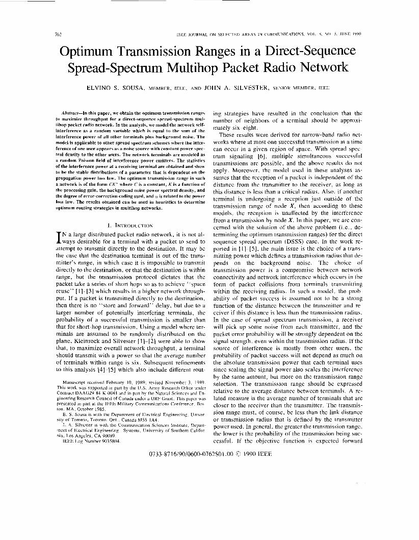
A weakness of the above model can be illustrated with the aid of Fig. 1 which depicts a network of four terminals

'The processing gain is equal to the ratio of the system bandwidth to the uncoded data rate (see 16. p. 13811.

Fig. I . The effect of transmission radius on interference

that use a constant (equal) power to communicate. If the transmitting power is such that the critical radius is deter- mined to be r,, then according to the model, terminals al and bl can successfully transmit to terminals u2 and b2, respectively, at the same time. However, if the powers are increased so that the critical radius becomes r-6, then the above two communications cannot occur simulta- neously. On the other hand, from a communication theory point of view, we know that the important parameter de- termining the success of a transmission is the signal-to- noise ratio at the receiver, which is not strongly depen- dent on the transmission power as long as all terminals transmit with the same power and the background noise is much smaller than the interference power.

The main drawback to the above model is that it does not discriminate between the differences in distance to a receiver of two transmitting terminals as long as the ter- minals are within the critical radius. An improved model is the capture model studied in [8]-[10], which is suited to FM transmission. If a given transmitting terminal, at distance rl from the receiver, is the closest transmitting terminal to the receiver, and if the next closest transmit- ting terminal is at a distance r2, then the given transmis- sion will be successful if rl < r, and the ratio r 2 / r I ex- ceeds a threshold called the capture ratio.

The above models have been used for the nonspread spectrum case. A straightforward extension of these models to spread spectrum would result by setting a threshold on the maximum possible number of successful simultaneous transmissions and declaring that any time the number of transmissions exceeds the threshold, all transmissions are lost. However, since the powers of the various interferers vary greatly due to differences in their distances to the receiver, the number of transmitting ter- minals is not a good variable to work with in accounting for network interference at a particular receiver. This is especially the case with DSSS signaling. The analysis presented in this paper is an enhancement of that in [ l 11 where we use the sum of the interference powers to model multiuser interference. This approach to interference modeling has been used in many analyses of cellular radio systems (e.g., [ 12]), spread spectrum multiple-access systems (e.g., [13]-[14]j, and has recently also been adopted for throughput analysis of packet radio networks with fixed topologies and prespecified routing schemes in 1151.

164 IEEE JOURNAL ( 3N SELECTED AREAS 1N COMMUNICATIONS, VOL 8. NO 5 . JUNE 1990

111. SYSTEM MODEL We assume a multihop packet radio network operating

under heavy traffic conditions. The system is slotted, and in each slot, a terminal transmits a packet with probability p . The slot duration is assumed to be sufficiently large so as to allow a preamble for spreading code and carrier syn- chronization. The traffic matrix is assumed to be uniform. We are interested in calculating performance over many different changing topologies rather than for a specific ter- minal configuration. As a result, we obtain statistical per- formance values over a set of topologies. To do this, we model the positions of the terminals as a Poisson point process in the plane with parameter A. If A is the area of a given region R in the plane, then the probability of find- ing k terminals in R is given by

CA”( P [ k in RI = (2 ) k!

where X is the average number of terminals per unit area. We assume that during each slot, the network topology is constant; hence, the interference level will be constant over a packet transmission time. We also assume that the interference is independent from slot to slot. This is the assumption that was made in [1]-[2] and other work that followed. With this assumption, we may apply the results to a network with dynamically changing topology or to obtain average performance results for a collection of ran- dom networks. In this work, we are interested in obtain- ing optimum transmission ranges; hence, we assume a prespecified link in the network with a given distance R. The objective is to optimize the expected forward prog- ress for a packet transmission as a function of the distance of the link in the presence of unknown network interferers that are modeled as a Poisson process. This philosophy is also consistent with the approach taken in [13] where a centralized system is analyzed.

IV. INTERFERENCE MODELING

The collision model for channel interference is not ap- plicable in the case of DSSS signaling or when interfering signals have small powers. An alternative model that is not usually used in the narrow-band packet radio network literature, but has been used in many analysis of DSSS systems such as in [12]-[14] is that of summing the in- terference powers and treating the total interference as Gaussian noise. At the network analysis level, many spread spectrum schemes may be modeled this way. In this paper, we assume a direct sequence scheme with bi- nary phase shift keying (DS/BPSK), although many other schemes such as DS/DPSK and the DPSK schemes that have been considered for cellular radio (e.g., [ 121) allow the same type of analysis.

From a network analysis viewpoint, we are usually in- terested in calculating the probability of packet success given that the receiver is idle. This calculation is usually conditioned on some state of the network, and a tractable state model cannot usually contain much more than infor-

mation on which terminals are transmitting and what are their received powers. A desirable model to work with in spread spectrum is the threshold model where we assume that the packet is successful if the signal to interference power ratio is greater than some threshold. To apply the threshold model, the variance of the interference at the detector must be directly related to the received interfer- ence power. In DS/BPSK systems with a large processing gain, it can indeed be shown that the noise at the detector due to one interferer is approximately Gaussian; however, the variance depends on the relative chip phase of the sig- nal to the interferer. For the case of many interfering sig- nals with approximately equal levels of interference, the chip phases average out and the noise variance is constant for a prespecified location of interferers. However, in some DS/BPSK system models with one strong interferer, the variance of the noise at the detector is a random vari- able that depends on the chip phase of the signal relative to the interferer. For a given total received power, the noise at the detector will have a variance that will vary from packet to packet. This variation can, however, be made small if there is an offset between the clocks of the various signals. We will assume this to be the case in this paper.

Threshold models in digital communications are ulti- mately dependent on the degree of error-correction cod- ing. If the interference over a packet can be modeled as Gaussian noise, then the probability of packet success as a function of the signal-to-interference ratio is a smooth curve with a slope in the transition region that depends on the degree of error correction; for good long codes, the curve approaches a step function. In this paper, we model the actual smooth curve.

To calculate the packet success probability, we assume that the level of interference is constant over the trans- mission of a packet. The noise at the detector is due to interference from other users and to a constant back- ground noise with power spectral density N 0 / 2 . We de- note the symbol energy-to-noise ratio at the detector by Eh/Noe f where N0,,/2 is an equivalent white noise power spectral density for the same SNR at the detector. If the received signal has power Po and the interferers have powers PI , P,, . * , P,, the average symbol energy-to- noise ratio at the detector in the case of DS/BPSK with rectangular chip pulse is then (see [16, eq. (17)] for a similar result with equal powers)

- I

p&(2K NOeff 3LP0 + - jO) ( 3 )

where L is the processing gain, Y = Cy=, P, , and vo = &/No. The parameter p0 is the SNR at the detector in the absence of interferers.

For a given p , the probability of symbol error is

p c = ierfc (4). (4)

The probability of packet success is dependent on the cod- ing scheme. We denote the probability of packet success

SOUSA A N D SILVESTER: OPTIMUM TRANSMISSION RANGES I N DSSS PACKET RADIO NETWORK

conditioned on the SNR p as s ( p ) . As an example, for a t-error-correcting block code of length n , and under our assumption that symbol errors are independent given p , we have

~ [ s u c c e s s / p ] A s ( p )

( 5 )

From packet to packet, the parameter p is a random vari- able with density functionf,( . ) . The unconditional prob- ability of packet success can then be written as

r m

r m

= I, [ l - F , ( x ) ] s’(x) CLX (6)

where the second expression is obtained after an integra- tion by parts and F,, ( . ) is the probability distribution function of p .

V. INTERFERENCE AT A GIVEN TERMINAL

To evaluate the above probability of packet success, we need to obtain the probability density function f, ( ) . We prefer, though, to obtain the probability density f y ( . ) first, i.e., the probability density function for the multi- user interference power. Towards this end, we may as- sume that the terminal at which we are interested in ob- taining the interference power is located at the origin.

Let g ( r ) be the power of a given signal at a distance r from the transmitter of the signal. In general, the exact form of g will depend on the environment; however, it will always be very large for small I’, and will approach zero as r + w. For the moment, though, so as not to restrict ourselves to any particular environment, we merely assume that g ( r ) satisfies the following two con- ditions:

1) g ( r ) is monotone decreasing, lim g ( r ) = 03, r - 0

and lim g ( r ) = 0 r+m

2) lim r 2 g ( r ) = 0. r + m

Without condition (7b), it can be shown that the interfer- ence power at a given terminal would be infinite for an infinite network. We will see later that in order for the characteristic function of the interference power to exist, we require that condition (7b) hold. The above expression for the power loss law is a far-field approximation that does not hold close to the transmitter where the transmit- ted signal attains a maximum. We assume that this max- imum is sufficient to cause a transmission error, even in the case of one interferer; hence, the above function will

result in the same probability of error while being easier to handle analytically.

Let X be a Poisson process in the plane with the average number of points per unit area equal to A. A sample func- tion of X is determined by a set of points in the plane which will correspond to locations of terminals. The probability law for X is determined by (2). We assume that the probability that a terminal is transmitting is p . The set of transmitting terminals also forms a Poisson process X‘ with parameter XI = Xp. Now, with each sam- ple function of X‘ , we can associate the random variable

Y = C g ( r i )

where the summation is over all the points of the sample function, and r, is the distance of the ith point to the ori- gin. We assume that each terminal (i.e., each point of the sample function) is transmitting. Thus, Y is the total in- terference power at the origin, and we wish to find its probability density.

Let Y, be the interference power received from those terminals which are in a disk or radius a , i .e. ,

r, c 11 (9)

Thus, we have 1imu-+- Y , = Y. We work with Yo and then let a + 00 to obtain the characteristic function of Y. The probability density function is then the inverse Fourier transform. Let be the characteristic function of Y , , i.e.,

$y,,(o) = E(elWY‘l 1. (10)

Using conditional expectations, this may be evaluated as

E ( eiWY“) = E ( E ( e fWy<’ /k in D , ) )

where “ k in D,” is the event that there are k terminals in the disk of radius a , and the expectation is over the ran- dom variable Yo.

Now, given that there are k points in D , , and due to the nature of the Poisson process, the distribution of their lo- cations is that of k independent and identically distributed points with uniform distribution. If R is the distance to the origin of a point that is uniformly distributed in Du, then the probability density of R is

f R ( T ) = [ a L 0 otherwise.

Also, since the characteristic function of the sum of a number of independent random variables is the product of the individual characteristic functions, we have

E ( e‘“‘/k in 0, ) =

Note that in (1 3 ) , we are considering U,, to be the sum of k random variables which are functions of the random

variables R;, and each Rj has the density given by (12). Thus, substituting (13) in (1 1) and summing the series, we obtain

Integrating by parts, the exponent of (14), letting a -+ 03,

and using condition (7a), we obtain, after some simplifi- cation, the characteristic function of Y

where g - ' ( . ) denotes the inverse of g ( ) .

A . Statistics for a Class of Propagation Laws To proceed further, we must now specify g ( r ) . We

specify it only up to a multiplicative constant since the results that we obtain will be independent of scaling fac- tors. In free space, g ( r ) would be l / v 2 ; however, this does not satisfy (7b). This means, as we will see shortly, that if we are going to assume the ideal law for g, then we cannot assume an infinite network, for the interference power would be strongly dependent on the network size. On the ground, g ( r ) takes the form l / r 4 [17]; thus, to work out this case and any other cases where the depen- dency on r is not exactly an inverse fourth power, we consider the following class of propagation laws:

For this class of propagation laws, (15) becomes

4 y ( w ) = exp ( i X t m j, t P e i w r d t ) (17)

where CY = 2 / y . The integral in (17) may be evaluated to obtain the following:

where r ( ) is the gamma function and 4 y ( U ) = 4; ( - U ) . The probability laws with characteristic func- tions given by (18) are the stable laws of exponent CY with the restriction 0 < CY < 1 [18]. For CY = 1 /2 , (18) be- comes

~ $ ~ ( w ) = exp (-nJ?r/2(1 - i ) X , & ) . (19)

This probability law (CY = 1 / 2 ) is the inverse Gaussian probability law, and is the only one of the stable laws, for the case 0 < a < 1, which is known to have a density given by a closed-form expression. The density for CY = 1 /2 is given by

and the distribution function is

In general, for 0 < CY < 1, the densities can be found as infinite series (see [18, pp. 581-5831). Let p = .rrh,r( 1 - a ) ; then the density, obtained by taking the inverse Fourier transform of (1 8), is

166 lEEE JOURNAL ON SELECTED AREAS I N COMMUNICATIONS. VOL 8. NO 5. JUNE 1990

which, for CY = 1 /2 , results in a series expansion for (20). The general distribution function is

VI. PROBABILITY OF PACKET SUCCESS

We assume a 1 / r4 propagation power loss law. Using the above distribution function for the interference, the probability of packet success is now computed. Let the distance between the transmitter and receiver be R. The signal power is then 1 /R4. The random variables Y and p are related through (3); hence, the probability distribution function for p may be obtained from that of Y in (21) as

where

K ( p ) = (; - ;). Substituting (24) in (6), we obtain the probability of packet success

In the above equation, K ( p ) + 1 may be interpreted as a multiple-access capability [ 141, in the case of equal interference powers, given the required SNR p at the de- tector [as can be seen from (3)]. The function s ' ( . ) de- pends on the level of coding. For the best long codes, this function approaches a delta function at some value of p , pLc. The integral can then be easily evaluated, and the re- sult corresponds to working with a reception model based on a threshold assumption. In any case, it can be seen that for the purpose of probability of packet success calcula- tions, we can always assume a threshold model. The above eauation gives the means to obtain the effective

SOUSA A N D SII.VE,STER. OPTIMUM TRANSMISSION RANGES IN DSSS PACKET RADIO NETWOKK 161

threshold, defined as the threshold, which when used with the threshold model, gives the same results as (25).

VII. OPTIMUM TRANSMISSION RANGES We are now ready to apply the above statistics of the

interference power to the determination of the optimum transmission range in a multihop network. First, we find an expression for nodal throughput as a function of the link distance R , the average number of terminals per unit area h. the transmission probability p , and the processing gain L.

A. Local Throughput The local throughput is the rate at which a terminal suc-

cessfully transmits packets. For a network with uniform traffic (as we assume here) and assuming that the routing is “balanced,” then the local throughput will be the same for all terminals. In terms of packets per slot, the local throughput will simply be the probability of success. Let [be the local throughput from terminal A , and let terminal B designate a generic destination terminal; then we have

[ = P I A transmits] . P [ B does not transmit]

. P [ packet received/B does not transmit].

Given that B does not transmit, it may not receive A’s transmission for one of the following two reasons: 1) B may receive a transmission from another terminal, or 2) the interference power at B may exceed the threshold. These two events are not strictly independent, and the ex- act calculation of the last factor of (26) is a difficult task. The lack of strict independence is due to the fact that if the interference power is large, then there is a greater probability of a large number of terminals in the vicinity of B. However, we will see shortly that the probability that B receives another transmission is weakly dependent on the number of terminals in the vicinity of B, and we may assume that the above two events are independent. If all terminals transmit with probability p (heavy traffic case), then the first two factors of (26) are given by p ( 1 - p ) . Now, due to the memoryless property of the Pois- son distribution, if we fix a transmitter and receiver, ter- minals A and B, the remaining terminals are still Poisson distributed with parameter A; thus, the probability of the second of the above events is simply P,7 and (26) becomes

B chooses

A’s transmission ~

To obtain the probability that B chooses A’s transmis- sion, we need to know how many terminals are transmit- ting to B. If k terminals (including A ) are transmitting to B, then we assume that the probability that B receives A’s transmission (assuming, of course, that B does not trans- mit and the interference power is less than the threshold) is I l k . The exact calculation that B chooses A’s trans- mission is very difficult. We do not know exactly how

many terminals are potential transmitters to B; and of the potential transmitters to B, we do not know the probabil- ity of a transmission to B from a given one of them. These parameters are tied to the results that we are trying to ob- tain. If the number of potential transmitters to B is n , and if we assume that each of these can transmit to n terminals (hence, the probability of a transmission to B is p / n ) , i.e., local traffic is uniform, then we have

B chooses

A’s transmission

where the summation results from conditioning on the number of transmissions addressed to B. Substituting (28) in (27), we obtain

(29)

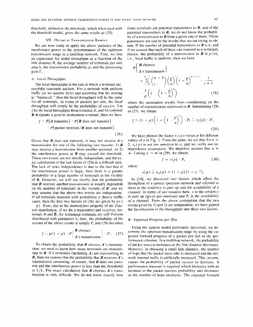
We have plotted the factor 7, ( p ) versus p for different values of rz in Fig. 2. From the plots, we see that for n > 2, ~ , , ( p ) is not too sensitive to n , and we verify our in- dependence assumption. We therefore assume that n = 03. Letting n + 00 in (29), we obtain

r = .(P> * p ,

~ ( p ) L 7 , ( p ) = ( I - p ) ( l - e - ” ) .

In [19], we discussed two factors which affect the throughput of a spread spectrum network and referred to them as the tendency to pair up and the availability of a channel. In terms of our notation here, 7 is the tendency to pair up (given per terminal) and P, is the availability of a channel. From the above assumption that the two events given by 1) and 2) are independent, we have gained the factorization of the throughput into these two factors.

(30)

where

B. Expected Progress per Slot

Using the system model previously described, we de- termine the optimum transmission range by using the ex- pected forward progress of a packet per slot as the per- formance criterion. In a multihop network, the probability of packet success increases as the link distance decreases. However, in choosing a small link distance, the number of hops that the packet must take is increased and the net- work internal traffic is artificially increased. This, in turn, causes the probability of packet success to decrease. A performance measure is required which increases with an increase in the packet success probability and decreases as the number of hops increases. The expected forward

768

0.28/ n:2

0.241

IEEE JOURNAL ON SELECTED AREAS IN COMMUNICATIONS, VOL. 8, NO, 5, JUNE 1990

K = l O

P

Fig. 2 . Tendency to pair up ~ , , ( p ) versus the probability of transmission P .

progress per slot [ 11-[5] is such a measure. The expected forward progress per slot Z is

Z = r - R . (31) To express the following results in terms of dimensionless quantities, we let N = X7rR2. N will be the average num- ber of terminals which are closer to A than B , and in terms of N, R = m. For the propagation law given by y = 4 ( i .e . , CY = 1 / 2 ) , we obtain the following [it results from substituting (30) in (31) and using (28) and (25)]:

AZ = - p ) ( l - e - p )

PROBABILITY OF TRANSMISSION

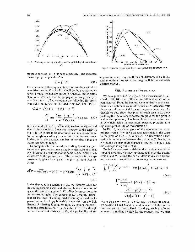
Fig. 3 . Expected progress per hop versus probability of transmission

We have multiplied Z by A in (32) so that the right-hand side is dimensionless. Note that contrary to the analysis in [ 11-[5], N is not to be interpreted as the average num- ber of neighbors of a given terminal ( A in our case). Rather, N is the average number of terminals that are within the chosen range.

To compute (32), we need the coding function s( p ) . As an example, we assume a highly coded system so that s ( . ) is close to a step function at some critical SNR which we denote as the parameter pc. The derivative is then ap- proximately given by s ’ ( p ) = 6 ( p - p c ) and (32) be- comes

(33) In the above, K is a function of pc, the required SNR for the coding scheme used, and also implicitly a function of po and the processing gain L . K is directly proportional to the processing gain. The parameter pc is mainly depen- dent on the level of coding, and assuming a fixed back- ground noise level, is mainly dependent on the link distance R. Setting K equal to zero, we obtain the maxi- mum link distance as Ro = ( Tx/( pcNo)) ‘I4. Even though the maximum link distance is R,, the probability of re-

ception becomes very small for link distances close to Ro, and an optimum transmission range will be considerably smaller than Ro.

VIII. PARAMETER OPTIMIZATION

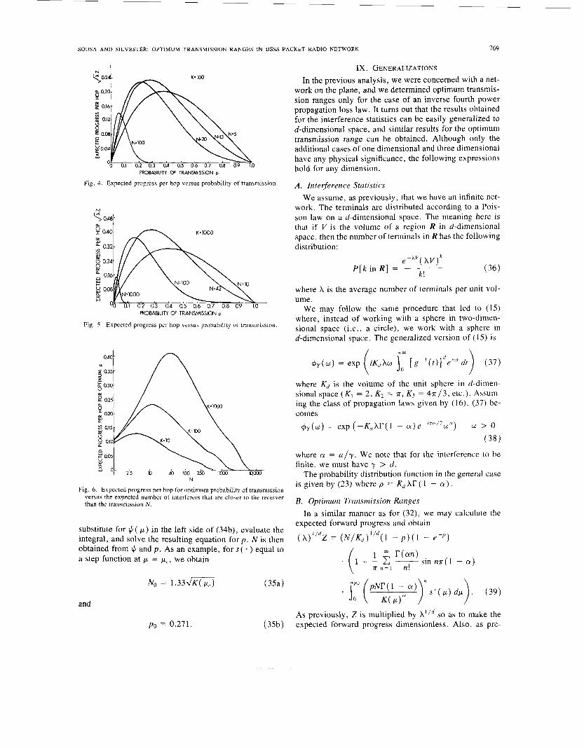
We have plotted (33) in Figs. 3-5 for the cases of K ( p c ) equal to 10, 100, and 1000 and for different values of the parameter N . From the figures, we note that in each case, there is an optimum value of N , and as N increases from this value, the expected forward progress decreases. Al- though we only show four plots for each case of K , the N yielding the maximum expected progress for the given K and at the optimum p has been chosen as the value over all N which yields the maximum expected progress at its optimum probability of transmission p .

In Fig. 6 , we show plots of the maximum expected progress versus N with K as a parameter, that is, the peaks in the plots of Figs. 3-5 versus N . An interesting obser- vation is the relation between the optimum N, that is, the N yielding the maximum expected progress in Fig. 6, and the corresponding value of K.

To find the parameters yielding the maximum expected forward progress, we may optimize (32) over the param- eters p and N . Setting the partial derivatives with respect to p and N to zero yields the following two equations:

2 (1 - p ) ( l - e - p ) (34b ) - -

&p[e-P(2 - p ) - 11

where $( p ) = ( p N / 2 ) d7r/K( p ) . To solve the above, we assume a fixed L and po, and then solve (34a) for the function $( p ) . For a fixed L and po, such a solution amounts to finding a value for the product p N . We then

SOUSA AND SILVESTER: OPTIMUM TRANSMISSION RANGES IN DSSS PACKET RADIO NETWORK

~

769

I

PROBABILITY OF TRANSMISSION p

Fig. 4. Expected progress per hop versus probability of transmission.

K:1000 - ROBABltlTY OF TRANSMISSION p

Fig. 5. Expected progress per hop versus probability of transmission.

Q40 - a

J Q35- 9 5 0.30- =

N

Fig. 6 . Expected progress per hop for optimum probability of transmission versus the expected number of interferers that are closer to the receiver than the transmission N .

substitute for $( p ) in the left side of (34b), evaluate the integral, and solve the resulting equation for p . N is then obtained from $ and p . As an example, for s ( ) equal to a step function at p = pc, we obtain

and

IX. GENERALIZATIONS In the previous analysis, we were concerned with a net-

work on the plane, and we determined optimum transmis- sion ranges only for the case of an inverse fourth power propagation loss law. It turns out that the results obtained for the interference statistics can be easily generalized to d-dimensional space, and similar results for the optimum transmission range can be obtained. Although only the additional cases of one dimensional and three dimensional have any physical significance, the following expressions hold for any dimension.

A . Interference Statistics We assume, as previously, that we have an infinite net-

work. The terminals are distributed according to a Pois- son law on a d-dimensional space. The meaning here is that if V is the volume of a region R in d-dimensional space, then the number of terminals in R has the following distribution:

e - ” “ ( h ~ ) ~ P [ k in RI = (36) k!

where h is the average number of terminals per unit vol- ume.

We may follow the same procedure that led to (15) where, instead of working with a sphere in two-dimen- sional space (i .e. , a circle), we work with a sphere in d-dimensional space. The generalized version of (15) is

C $ ~ ( W ) = exp iKdhw [ g - l ( t ) ] d e ’ w ‘ dr ( 1, where Kd is the volume of the unit sphere in d-dimen- sional space ( K , = 2, K2 = T , K3 = 47r/3, etc.). Assum- ing the class of propagation laws given by (16), (37) be- comes

~ $ ~ ( o ) = exp ( -Kdxr( 1 - a ) e - ’ T e / 2 0 U ) w > o (38)

where a = a/-y. We note that for the interference to be finite, we must have y > d.

The probability distribution function in the general case is given by (23) where p = K,, AT ( 1 - a).

B. Optimum Transmission Ranges

expected forward progress and obtain

( x ) ” ~ z = (N/K, ) ’ ’~ ( I - p ) ( l - e-”)

In a similar manner as for ( 3 2 ) , we may calculate the

As previously, Z is multiplied by A l l d so as to make the expected forward progress dimensionless. Also, as pre- PO = 0.271. (35b)

770 IEEE JOIJRNAL. ON SELECTED AREAS IN COMMUNICATIONS, VOL.. X. NO. 5 . JUNE 1990

TABLE 1 SOMI: OF T H ~ CONSTANTS I N (40)

I C (d. a) I

viously, we would like to find the optimum N as a func- tion of K and for the optimum transmission probability p . We may optimize over the parameters p and N as before. For the case of a step coding function s ( ) , we summa- rize the results as follows: for a given d and CY, the opti- mum transmission range No is given by the relation

As previously, No is proportional to a power of the param- eter K ( p c ) . We give a few values of the constant C in Table I .

We summarize the above results. In obtaining the in- terference statistics, the important parameters are d, the dimension of the network, and y, the exponent of the propagation loss law. Given these two parameters. we de- fine CY = d / y . The interference statistics are then given by the stable law of exponent CY, and the optimum No is proportional to K N ( p, . ) where K ( * ) is defined as in (24) and Table I gives a few of the proportionality constants.

X. SUMMARY A N D CONCLUSIONS Multihop packet radio models used in the past have used

the concept of a transmission radius where within a given radius of a transmitter, a packet has an “equal” prob- ability of being received. This model essentially assumes a step function for the signal strength versus distance from the transmitter. In this paper, we have taken a new ap- proach: a signal is assumed to decay in strength according to a gradually decreasing function of the distance from the transmitter. By assuming a random distribution of the ter- minals, we were able to obtain the statistics of the inter- ference power from all other transmissions at a particular receiver. Assuming an inverse power law for the signal strength versus distance from the transmitter, we showed that the probability laws of the interference power are the stable laws with parameter CY restricted to 0 < CY < 1. The case of an inverse fourth power propagation law, which results from ground wave propagation, corresponds to the stable law with CY = 1/2, which has a density known as the inverse Gaussian probability density.

In a multihop packet radio network, there is usually a tradeoff between the distance covered in one hop and the probability of a successful transmission. Using the above interference analysis, we proceeded to obtain the opti- mum transmission range for a DSSS network. For a nar- row-band packet radio network, previous results have concluded that the range of a transmission should be such that on the average there are approximately six-eight ter-

minals closer to the transmitter than the receiver. For a spread spectrum system, we expect different results since multiple simultaneously successful transmissions are pos- sible. In the spirit of the analysis of Kleinrock and Silves- ter [1]-[3], we have concluded that in a direct sequence spread spectrum network, the range of a transmission should be chosen so that on the average there are 1.33

terminals closer to the transmitter than the re- ceiver where K ( p ( . ) is a parameter that is proportional to the processing gain, which can be interpreted as the effec- tive maximum number of simultaneously successful trans- missions possible in some region as a function of the ef- fective SNR pf. required for a particular coding scheme.

REFERENCES 111 L. Kleinrock and J. A. Silvester, “Optimum transmission radii for

packet radio networks or why six is a magic number,” in Cor~f. Rrc.. Nul. Telecwmrnun. Conf , Dec. 1978, pp. 4.3. 1-4.3.5.

[2] J . A. Silvester, “On the spatial capacity of packet radio networks,’’ Dep. Comput. Sci., U n i v . California, Los Angeles. Eng. Rep. UCLA- ENG-8021. May 1980.

131 L . Kleinrock, and J . A. Silvester, “Spatial reuse in multihop packet radio networks.” Proc. IEEL’, vol. 75, pp. 116-134, Jan. 1987.

141 H. Takagi and L. Kleinrock, “Optimal transmission ranges for ran- domly distributed packet radio terminals.” IEEE Truns. Coinrnun.. vol. COM-32. pp. 264-257, Mar. 1984.

[SI T. C. Hou and V. 0. K. Li, “Transmission range control in multihop packet radio networks,’’ IEEE Trails. Cornrnun.. vol. COM-34, pp. 38-44, Jan. 1986.

161 M. ti. Simon, J . K. Onium, R. A. Scholtz. and B. K . Levitt, Sprrrrd Sprcrrurn Coiirrrrunic.crrion.c, Vol . 1. Rockville, MD: Computer Sci- ence Press, 1984.

171 W. C . Peng, “Some communication jamming games.” Ph.D. dis- sertation, Dep. Elec. Eng.. Univ. Southern California, Los Angeles. Jan. 1986.

[8] L. G. Roberts, “ALOHA packet system with and without slots and capture,” ARPA Network Inlorni. Cen., Stanford Res. Inst., Menlo Park, CA, ASS Note 8 (NIC 11290). June 1972; reprinted in C O ~ ~ / J U / . Cornnrun. Rei,. , vol. 5, pp. 28-42, Apr. 1975.

[91 L. Fratta and D. Sant, “Some models of packet radio networks with capture,” in Proc. In/. Con$ Compur. Coinmun., Oct. 1980, pp. 155- 161.

I O ] R. Nelson and L. Kleinrock, “The spatial capacity of a slotted ALOHA multihop packet radio network with capture,” Cornrnun., vol. COM-32. pp. 684-694. June 1984.

1 I ] E. S. Sousa and J . A. Silvester. “Determination of optimum trans- mission ranges in it multi-hop spread spectrum network.” in Proc. MILCOM. Boston, MA, Oct. 1985, pp. 449-454.

121 Ci. R . Cooper and R. W. Nettleton, “A spread-spectrum technique for high capacity mobile communications,“ IEEE Trcr17.c. V r h i c . Techno/ . . vol. VT-27, Nov. 1978.

[13] S . A. Musa and W. Wasylkiwskyj. “Co-channel inference of spread spectrum systems in a multiple user environment.” IEEE Truns. Coniniun.. vol. COM-26, pp. 1405-1413, Oct. 1978.

[I41 C . L. Weber, G. ti. Huth, and B. H. Batson. ”Performance consid- eration of code division multiple-access systems,” IEEE Truns. Vrhic . T ~ k n o l . . vol. VT-30, pp. 3-9, Feb. 1981.

[I51 0. DeSouza, P. Sen, and R. R. Boorstyn, “Performance analysis of spread spectrum packet radio networks.” in Proc. MILCOM. San Diego. CA. Oct. 1988, pp. 599-604.

161 M. B. Pursley, “Performance evaluation for phase-coded apread- spectrum multiple-access communication-Part I: System analysis,” IEEE Truns. Corninrtn.. vol. COM-25 pp. 795-799, Aug. 1977.

171 J. J . Egli. “Radio propagation above 40 Mc over irregular terrain,” Proc. IRE , pp. 1383-1391. Oct. 1957.

181 W. Feller, A n 1nrroduc.rion r o Prohabiliry Throry crnd I t s Applicu- t i o r i s , Vol . I / .

191 E. S . Sousa and J . A. Silvester, “Spreading code protocols for dis- tributed spread spectrum packet radio networks,’’ /EEL‘ Trans. Corn- i n u n . . vol. 36, pp. 272-281. Mar. 1988.

Wiley, 1966, pp. 554-583.

SOUSA AND SILVESTER: OPTIMUM TRANSMISSION RANGES IN DSSS TACKET RADIO NETWORK 77 1

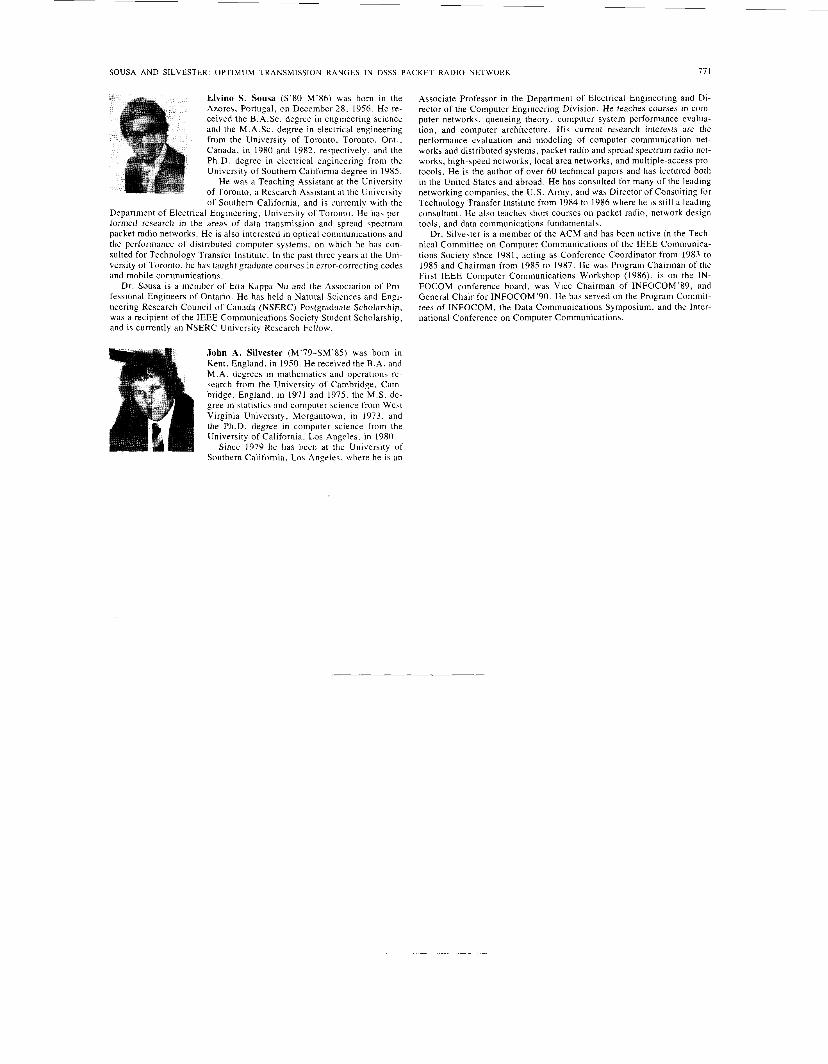
Elvino S. Sousa (S’80-M’86) was born in the Azores, Portugal, on December 28, 1956 He re- ceived the B A.Sc degree in engineering science and the M A Sc degree in electrical engineering from the University of Toronto, Toronto, Ont , Canada, in 1980 and 1982, respectively, and the Ph D degree in electrical engineering from the University of Southern California degree in 1985

He was a Teaching Assictant at the University of Toronto, a Research Awstant at the Univenity of Southern California, and 15 currently with the

Department of Electrical Engineering, University of Toronto. He has per- formed research in the areas of datd transmission and spread spectrum packet radio networks He is also interested in optical communications and the performance of distributed computer systems, on which he has con- culted for Technology Transfer Institute In the pa51 three yearc at the Uni- versity of Toronto, he has tdught graduate courfe\ in error-correcting code\ and mobile communications

Dr Sousa is a member of Etta Kappa Nu and the ASwcidtion of Pro- fewonal Engineers of Ontario He has held a Natural Sciences and Engi- neering Research Council of Canada (NSERC) Postgraduate Scholarship, was a recipient of the IEEE Communications Society Student Scholarship, and is currently an NSERC University Research Fellow

John A. Silvester (M’79-SM’85) was born in Kent, England, in 1950. He received the B.A. and M.A. degrees in mathematics and operations re- search from the University of Cambridge, Cam- bridge, England, in 1971 and 1975, the M.S. de- gree in statistics and computer science from West Virginia University, Morgantown, in 1973, and the Ph.D. degree in computer science from the University of California, Los Angeles, in 1980.

Since 1979 he has been at the University of Southern California, Los Angeles, where he is an

Associate Professor in the Department of Electrical Engineering and Di- rector of the Computer Engineering Division. He teaches courses in com- puter networks, queueing theory, computer system performance evalua- tion, and computer architecture. His current research interests are the performance evaluation and modeling of computer communication net- works and distributed systems, packet radio and spread spectrum radio net- works, high-speed networks, local area networks, and multiple-access pro- tocols. He is the author of over 60 technical papers and has lectured both in the United States and abroad. He has consulted for many of the leading networking companies, the U.S. Army, and was Director of Consulting for Technology Transfer Institute from 1984 to 1986 where he is still a leading consultant. He also teaches short courses on packet radio, network design tools, and data communications fundamentals.

Dr. Silvester is a member of the ACM and has been active in the Tech- nical Committee on Computer Communications of the IEEE Communica- tions Society slnce 1981, acting as Conference Coordinator from 1983 to 1985 and Chairman from 1985 to 1987. He was Program Chairman of the First IEEE Cornputer Communications Workshop (1986), is on the IN- FOCOM conference board. was Vice Chairman of INFOCOM’89, and General Chair for INFOCOM’90. He has served on the Program Commit- tees of INFOCOM, the Data Communications Symposium, and the Inter- national Conference on Computer communications.