Option Prices and the Probability of Success of Cash … Prices and the Probability of Success of...

Option Prices and the Probability of Success of

Cash Mergers

C. Alan Bester, Victor H. Martinez, and Ioanid Rosu∗

February 15, 2011

Abstract

When a cash merger is announced but not yet completed, there are two key unob-

served variables involved in the target company stock price: the probability of success,

and the fallback price, i.e., the price conditional on merger failure. We propose an

arbitrage-free model involving these two sources of uncertainty which prices European

options on the target company. We empirically test our formula in a study of all cash

mergers between 1996 and 2008. The formula matches well the observed volatility smile.

Furthermore, as predicted by the model, we show empirically that the volatility smile

displays a kink, and that the kink is proportional to the risk-neutral probability of deal

success.

JEL Classification: G13, G34.

Keywords: Mergers and acquisitions, Black–Scholes formula, success probability, fall-

back price, Markov Chain Monte Carlo.

∗Bester is with the University of Chicago, Booth School of Business; Martinez is with CUNY BaruchCollege, Zicklin School of Business; Rosu is with HEC Paris. We have benefited from discussions withMalcolm Baker, John Cochrane, George Constantinides, Doug Diamond, Pierre Collin-Dufresne, CharlotteHansen, Steve Kaplan, Jun Pan, Monika Piazzesi, Lubos Pastor, Ajay Subramanian, Pietro Veronesi; seminarparticipants at Chicago Booth, Courant Institute, CUNY, Princeton, Toronto, Lausanne; and conferenceparticipants at the AFA meetings, 2010.

1

1 Introduction

One of the most common violations of the Black–Scholes formula is the volatility smile, a

pattern in which at-the-money options have lower implied volatilities than in-the-money or

out-of-the-money options. The U.S. option markets have been displaying a volatility smile

since the October 1987 market crash. This has been widely attributed to the market’s chang-

ing its assumption of a log-normal distribution of equity prices to account for the small

probability of a large market crash.1

Another example of a non-log-normal distribution is when the underlying company is the

target of a merger attempt.2 In a typical merger, a company A, the acquirer, makes an

offer to a company B, the target. The offer can be made with A’s stock, with cash, or a

combination of both. The offer is usually made at a significant premium compared with B’s

pre-announcement stock price. Therefore, the distribution of the stock price of B is bi-modal:

if the deal is successful, the price rises to the offer price; if the deal is unsuccessful, the price

reverts to a fallback price.3

In this paper we focus on cash mergers, which are defined as mergers for which the offer

is made exclusively in cash. We do that for two reasons. One is that, when studying options

on the target company, as a first approximation we can ignore the stock price of the acquirer;

this leads to a simpler model. The second reason is that the price distribution of the target

company in a cash merger is further away from the log-normal distribution than in the case

of stock-for-stock or hybrid mergers; this gives us more power in understanding departures

from the Black–Scholes formula.

Our model proposes an arbitrage-free formula that prices options on the target company

of a cash merger. We depart from the Black–Scholes formula by focusing on the two main

uncertainties surrounding the merger: the success probability and the fallback price. We test

our formula in a study of all cash mergers during the 1996–2008 period with sufficiently liquid

1Black and Scholes (1973) assume that the underlying equity price follows a log-normal distribution withconstant volatility, which means that the implied volatilities should be the same, irrespective of the strikeprice of the option. Rubinstein (1994) and Jackwerth and Rubinstein (1996) show that the volatility smileafter the 1987 crash implies a significant violation of the log-normal distributional assumption.

2Black (1989) points out that the Black–Scholes formula is unlikely to work when the company is thesubject of a merger attempt.

3The fallback price reflects the value of the target firm B based on fundamentals, but also based on otherpotential merger offers. The fallback price therefore should not be thought as some kind of fundamental priceof company B, but simply as the price of firm B if the current deal fails.

2

options traded on the target company. We find our model produces pricing errors 21% smaller

on average than the Black–Scholes formula.

Further analysis shows that our theoretical volatility smile is in close agreement with

the one observed in the data. In particular, our formula predicts that the volatility smile

should display a kink when the strike price equals the cash merger offer price. Moreover, the

magnitude of the kink (i.e., the difference between the slope of the volatility smile above and

below the offer price) should be proportional to the risk-neutral success probability. Empirical

results indicate that this prediction is strongly supported in the data. Our model also explains

why, as we observe in the data, the Black–Scholes implied volatility decreases when the deal

is close to being successful: a success probability close to one leads to an implied volatility

close to zero.

To our knowledge, our paper is the first to study option pricing on mergers by allowing

the success probability to be stochastic. This has the advantage of being realistic: many news

stories before the resolution of a merger refer only to the success probability of the merger.

A practical advantage is that by estimating the whole time series of the success probability,

we can estimate the merger risk premium and the merger volatility (i.e., the volatility of the

success probability). Also, our model is well suited to study cash mergers, which are difficult

to analyze with other models of option pricing. Subramanian (2004) proposes a jump model

of option prices on stock-for-stock mergers. According to his model, initially the price of each

company involved in a merger follows a process associated to the success state, but may jump

later at some Poisson rate to the process associated to the failure state. This approach cannot

be extended to cash mergers: when the deal is successful, the stock price of the target becomes

equal to the cash offer, which is essentially constant; thus, the corresponding process has no

volatility. In our model, the price of the target is volatile: this is due to both a stochastic

success probability and a stochastic fallback price.

Conceptually, our model resembles a dynamic version of the classical Arrow-Debreu frame-

work of state-contingent prices, in which the probabilities corresponding to the two states

(success and failure) are stochastic. In principle, our model could also be extended to stock-

for-stock mergers. Subramanian (2004) assumes that the price processes associated to the

success state for the aquirer and the target companies are perfectly correlated. This is not

a realistic assumption when the merger has a low success probability. Moreover, his model

3

implies that the success probability of a merger decreases deterministically with time, even

when the merger is likely to succeed. Samuelson and Rosenthal (1986) find empirically that

the success probability usually increases over time.

To set up our model, consider the target company of a cash merger. If the deal is successful,

the target company’s shareholders receive a fixed offer price per share, B1. If the deal fails,

the share price the target reverts to a fallback price, B2. We assume that B2 has a log-normal

distribution. We also assume that the success probability of the deal follows a stochastic

process. As in the martingale approach to the Black–Scholes formula, instead of using the

actual success probability, we focus on the risk-neutral probability, q.4 When the success

probability, q, and the fallback price, B2, are uncorrelated, our formula takes a particularly

simple form.

Our option formula relates the latent (unobserved) variables, q and B2, to the observed

variables: the price of the target company, B, and the prices of the various existing options

on B. Since the Black–Scholes formula is non-linear in the stock price, we need a statistical

technique that deals with non-linear formulas and identifies both the values of the latent

variables and the parameters that generate the processes. The method we use is called the

Markov Chain Monte Carlo (MCMC).5 Though this algorithm is flexible enough to allow

us to use any (or all) options traded on the stock, for simplicity we choose only one option

each day, e.g., the call option with the maximum trading volume on that day. As we discuss

later, this choice also allows us to perform specification checks on our model, including out of

sample pricing of options with different strike prices.

We apply the option formula to all cash mergers during the 1996–2008 period with suffi-

ciently liquid options traded on the target company. After removing companies with illiquid

options, we obtain a final sample of 282 cash mergers. We test our model in three different

ways. First, we compare the model-implied option prices to those coming from the Black-

4In the absence of time discounting, the risk-neutral probability q(t) would be equal to the price at t of adigital option that offers $1 if the deal is successful and $0 otherwise.

5For a discussion of Markov Chain Monte Carlo methods in finance, see the survey article of Johannes andPolson (2003). MCMC methods allow us to conduct inference by sampling from the joint distribution of modelparameters and unobserved state variables (in this case q and B2) given the observed data. MCMC methods forstate space models are well established in Bayesian statistics and econometrics (see, e.g., Jacquier, Johannes,and Polson (2007)). MCMC is particularly convenient here because some parameters enter the model non-linearly, meaning standard techniques for latent variable models, such as the Kalman filter, would need to bemodified. We emphasize that this choice is based on convenience and that many other estimation approaches(frequentist and Bayesian) are possible.

4

Scholes formula, and we investigate the volatility smile. Since our estimation method uses

one option each day, we check whether the prices of the other options on that day—for differ-

ent strike prices—line up according to our formula. Second, we explore whether the success

probabilities uncovered by our approach predict the actual deal outcomes we observe in the

data. Finally, we explore the implications of our model for the volatility dynamics and risk

premia associated with mergers.

In comparison with the Black–Scholes formula with constant volatility, our option formula

does significantly better: the median percentage error is 26.06% for our model compared to an

error of 33.02% in the case of the Black–Scholes model.6 Our formula also does well compared

to a modified Black–Scholes formula in which the volatility equals the previous-day implied

volatility at the same strike price. This modified Black–Scholes formula is very difficult to

surpass, as it already incorporates the observed volatility smile from the previous day. Even

though we use only one option each day in our estimation process, our out-of-sample option

pricing estimates are very close to the observed prices and therefore produce a volatility smile

close to the observed one.

We test the implications of the model regarding the kink in the volatility smile. If instead

of looking at the volatility plot we consider plotting the call option price against the strike

price, then theoretically the magnitude of the kink normalized by the time discount coefficient

should be precisely equal to the risk-neutral probability. A regression of the normalized kink

on the estimated risk-neutral probability strongly supports the prediction that the intercept

equals to 0 and the slope equals to 1. Our estimation procedure uses only one option each day,

yet it matches well the whole cross section of options for that day, including the magnitude

of the kink.

We show that the probabilities estimated using our formula predict the outcomes of deals

in the data. In particular, this method does significantly better than the “naive” method

widely used in the mergers and acquisitions literature, which estimates the success probability

based on the distance between the current stock price and the offer price in comparison to

the pre-announcement price.

We also investigate how the fallback price compares to the price before the announce-

ment. One might expect that the fallback price should be on average higher than the pre-

6The error is smaller than the average bid-ask spread for options in our sample.

5

announcement price. This may be due to the fact that a merger is usually a good signal

about the quality of the target company, and indicate that other takeover attempts are now

more likely. We find that indeed the fallback price is on average 27% higher than the pre-

announcement price.

Another implication of our model is that the merger risk premium may be estimated as

the drift coefficient in the diffusion process for the success probability. This is individually

very noisy, but over the whole sample the estimated merger risk premium is significantly

positive, at an 158% annual rate (with an error of ±29%). This figure is comparable to the

one obtained by Dukes, Frolich and Ma (1992), which examine arbitrage activity around 761

cash mergers between 1971 and 1985 and report returns to merger arbitrage of approximately

0.47% daily. See also Mitchell and Pulvino (2001) and Jindra and Walkling (2004) for a more

detailed discussion of the risks and the transaction costs involved in merger arbitrage.

Background Literature

The literature on option pricing for companies involved in mergers is scarce. Moreover, with

the exception of Subramanian (2004), which has been discussed above, the literature has

mostly been on the empirical side.7

Samuelson and Rosenthal (1986) is close in spirit to our paper. They start with an

empirical formula similar to our Equation (7), although they do not distinguish between

risk-neutral and actual probabilities. Assuming that the success probability and fallback

prices are constant (at least on some time-intervals), they develop an econometric method

of estimating the success probability.8 The conclusion is that market prices usually reflect

well the uncertainties involved, and that the market’s predictions of the success probability

improve monotonically with time.

Brown and Raymond (1986) reflect the widely spread practice in the industry of measuring

the success probability of a merger by taking the fallback price to be the price before the deal

was announced. We call this the “naive” method of estimating the success probability. We

show that our method does better than the naive method.7For a theoretical discussion about preemptive bidding, and an explanation of the offer premium or the

choice between cash deals and stock deals, see Fishman (1988, 1989).8They estimate the fallback price by fitting a regression on a sample of failed deals between 1976–1981.

The regression is of the fallback price on the offer price and on the price before the deal is announced.

6

Barone-Adesi, Brown, and Harlow (1994) point out that option prices are useful for ex-

tracting information about mergers. Hietala, Kaplan, and Robinson (2003) discuss the dif-

ficulty of information extraction around takeover contests, and estimate synergies and over-

payment in the case of the 1994 takeover contest for Paramount in which Viacom overpaid

by more than $2 billion.

Several articles focus on the information contained in asset prices prior to mergers. Cao,

Chen, and Griffin (2005) observe that option trading volume imbalances are informative prior

to merger announcements, but not in general. From this, along the lines of Ross (1976), they

deduce that option markets are important, especially when extreme informational events are

pending. McDonald (1996) analyzed option prices on RJR Nabisco, which was the subject of

a hostile takeover between October, 1988 and February, 1989, and noticed that there was a

significant failure of the put–call parity during that time.

Mitchell and Pulvino (2001) survey the risk arbitrage industry and show that risk arbitrage

returns are correlated with market returns in severely depreciating markets, but uncorrelated

with market returns in flat and appreciating markets. This correlation shows that there is a

positive merger risk premium.

There is also a related literature on pricing derivative securities under credit risk. The

similarity with our framework lies in that the processes related to the underlying default are

modeled explicitly, and their estimation is central in pricing the credit risk securities. See,

e.g., Duffie and Singleton (1997), Pan and Singleton (2008), Berndt et al. (2005). Similar

ideas to ours, but involving earning announcements can be found in Dubinsky and Johannes

(2005), who use options to extract information regarding earnings announcements.

The paper is organized as follows. Section 2 describes the model, and derives our main

pricing formulas, both for the stock prices and the option prices corresponding to the stocks

involved in a cash merger. Section 3 presents the empirical tests and the simulations of our

model, and Section 4 concludes.

7

2 Model

2.1 Theory

Consider a company A, the acquirer, which announces at t = 0 that it wants to merge with

a company B, the target. The acquisition is to be made with B1 dollars in cash per share.

At some fixed future date, Te, called the effective date, the uncertainty about the merger is

resolved. The effective date is known in advance by all market participants. If the merger

succeeds, on the effective date the target firm’s shareholders receive B1 per share; if the merger

fails, they receive B2 per share.

At each t between 0 and Te, define by pm = pm(t) the market price of a contract that pays

$1 if the merger goes through or $0 if the merger fails.9 Also, define the fallback price, B2(t),

to be the value of the target company estimated by the market at t, conditional on the merger

not being successful. Both B2 and pm are public information. To allow for generalizations,

we assume that the offer price, B1, is also stochastic. Later, we analyze the case when B1 is

constant.

Let W (t) be a 3-dimensional standard Brownian motion on a probability space (Ω,F , P ).

We assume that B1(t), B2(t) are log-normal diffusion processes with constant drift and volatil-

ity: Bi(t) = eXi(t), with dXi(t) = µi dt + σi dWi(t), i = 1, 2. Also, pm(t) is an Ito process

given by dpm(t) = µpm(t), t

dt + σ

pm(t), t

dW3(t), where µ and σ satisfy regularity con-

ditions as in Duffie (2001), and are such that pm is always between 0 and 1.10 The process

pm is independent of B1 and B2.11

Denote by β(t) = ert the price of the bond (money market) at t. Denote by Q the

equivalent martingale measure associated to B1, B2, pm. This is done as in Chapter 6 of

Duffie (2001), except that we want B1, B2, pm to be Q-martingales after discounting by β.

At each t, denote

q(t) = pm(t) er(Te−t) . (1)

9If a futures contract betting on the success of the merger were traded on the Iowa Electronic Markets orIntrade, pm(t) would be the market price of this contract.

10We could require that on the effective date pm(Te) be either 0 or 1, but we prefer the more general casewithout any such restriction. The intuition is that even on the effective date the market may be uncertainabout the outcome of the merger, so at the beginning of the effective date it assigns the probability pm(Te).

11The case when pm is correlated with B2 is discussed after Theorem 1. Since later we treat B1 as deter-ministic, we do not explicitly discuss the case when q and B1 are correlated. This latter case can be solvedusing similar methods.

8

The process q(t) is the risk-neutral probability of the state in which the merger succeeds.

Because pm(t) is a discounted martingale with respect to Q, we have

EQt

pm(Te)

β(Te)

=

pm(t)

β(t)or, equivalently, EQ

t q(Te) = q(t). (2)

We extend the probability space Ω on which Q is defined by including the binomial jump

of pm on the effective date. Since we want pm = 1 at the end of the effective date, we

require that pm jump to 1 with probability pm(Te). This defines a new equivalent martingale

measure Q and a new filtration F . Denote by T e the instant after Te at which we know

whether pm equals 1 or 0. Extend pm as a stochastic process on [0, Te] ∪ T e by including

the jump. We note that pm = q at both Te and T e, so the payoff of B at T

e can be written as

q(T e)B1(T

e)+ (1− q(T e))B2(T

e), since q(T e) is either 1 or 0 depending on whether the merger

is successful or not.

We are in the position to apply Theorem 6J in Duffie (2001) for redundant securities.

Markets are dynamically complete before Te, because the uncertainty stems from the three

Brownian motions involved in the definition of the securities B1, B2, pm. Moreover, at Te,

the stock price has a binary uncertainty that can be spanned only by the bond and pm.

Then, in the absence of arbitrage, any other security whose payoff depends on B1, B2, pm is a

discounted Q-martingale. In particular, the price of the target company B(t) is a discounted

Q-martingale. But, as discussed above, B(T e) = q(T

e)B1(T e)+(1−q(T

e))B2(T e). This allows

us to derive the formula for B(t) in Theorem 1.

Consider also a European call option on B with strike price K and maturity T ≥ Te.

Denote by C(t) its price, and by X+ = maxX, 0. Denote by C2(t) the theoretical Black–

Scholes price of a European call option on B2 with strike price K and maturity T . When

B1 is stochastic, denote by C1(t) the price of a European call option on B1 with strike price

K and maturity Te. Under the assumption that the diffusion and volatility parameters are

constant, the option price C2(t) satisfies the Black–Scholes formula:

C2(t) = CBS(B2(t), K, r, T − t,σ2) = B2(t)N(d1)−K e−r(T−t) N(d2), (3)

d1,2 =log(B2(t)/K) + (r ± 1

2σ22)(T − t)

σ2

√T − t

. (4)

9

We can now derive the following result.

Theorem 1. Assume q, B1, B2 satisfy the assumptions made above, with q is independent

from B1 and B2. Then, if B1 is stochastic the target stock price and option price satisfy

B(t) = q(t)B1(t) + (1− q(t))B2(t). (5)

C(t) = q(t)C1(t) + (1− q(t))C2(t). (6)

If B1 is constant the formulas become

B(t) = q(t)B1 e−r(Te−t) +(1− q(t))B2(t). (7)

C(t) = q(t)(B1 −K)+ e−r(Te−t) +(1− q(t))C2(t). (8)

Proof. See the Appendix.

If q and B2 are correlated, one can still obtain similar results, but the formulas are

more complicated. To see where the difficulty comes from, suppose B1 is constant. Let

us consider the derivation of the formula for B(t) in the proof of the Theorem: B(t) =

β(t)β(Te)

EQt

q(Te)B1 + (1− q(Te))B2(Te)

. The problem arises when attempting to calculate the

integral EQt

q(Te)B2(Te)

. This is in general a stochastic integral, but in particular cases it

can be reduced to an indefinite integral in two real variables.

Now we study the Black–Scholes implied volatility curve under the hypothesis that our

model is true. The volatility curve plots the Black–Scholes implied volatility of the call option

price against the strike price K. If the Black–Scholes model were correct, the curve would

be a horizontal line, indicating that the implied volatility should be a constant: the true

volatility parameter. But in practice, as observed by Rubinstein (1994), the plot of implied

volatility against K is convex, first going down until the strike price is approximately equal to

the underlying stock price (the option is at-the-money), and then going up. This phenomenon

is called the volatility “smile” or, if the curve is always decreasing, the volatility “smirk.”

The next result shows that, in the case of options on cash mergers, the volatility smile arises

naturally if the merger success probability is sufficiently high. Our model implies that the

volatility curve is convex, with a kink at K = B1, the offer price. The magnitude of the kink

(the difference between the slope of the curve on the right and left of K = B1) equals the time-

10

discounted risk-neutral probability, divided by the option vega. According to Equation (4),

d2 = d2(S, K, r, τ, σ) =log(S/K)+(r−1

2σ2)τ

σ√

τ , with τ = T − t. Denote by ν = ν(S, K, r, τ, σ) = ∂C∂σ

the option vega; and by χ(·) the indicator function: χ(x) = 1 if x > 0 and χ(x) = 0 otherwise.

Proposition 1. If the offer price B1 is constant, the slope of the implied volatility plot equals

∂σimp

∂K= e−rτ

ν(B,K,r,τ,σimp)

−q(t)χ(B1−K)−(1−q(t))N

d2(B2, K, r, τ, σ2)

+N

d2(B, K, r, τ, σimp)

,

where ν = ∂C∂σ is the option vega. For q(t) sufficiently close to 1 the slope

∂σimp

∂K

K↑B1

is

negative and the slope

∂σimp

∂K

K↓B1

is positive. The magnitude of the kink, i.e., the slope

difference equals

∂σimp

∂K

K↓B1

−

∂σimp

∂K

K↑B1

=e−rτ q(t)

ν(B, K, r, τ, σimp). (9)

Proof. The formula for ∂σimp

∂K comes from differentiating with respect to K our option pricing

formula for cash mergers: C(t) = q(t) e−rτ (B1 − K)+ + (1 − q(t))CBS(B2(t), K, r, τ, σ2) =

CBS(B, K, r, τ, σimp). This also implies the formula for the magnitude of the kink. Moreover,

we get the following formula:

∂C

∂K

K↓B1

−

∂C

∂K

K↑B1

= e−rτ q(t). (10)

Note that

∂σimp

∂K

K↑B1

is proportional to −q − (1 − q)N(d2,B2) + N(d2,B), which is negative

for q sufficiently close to 1. Also,

∂σimp

∂K

K↓B1

is proportional to −(1− q)N(d2,B2) + N(d2,B),

which is positive for q sufficiently close to 1.

In fact, one can check numerically that

∂σimp

∂K

K↑B1

is negative and

∂σimp

∂K

K↓B1

is positive

for most of the relevant values of the parameters. This implies the usual convex shape for the

volatility smile.

Now we prove a result about the instantaneous volatility that will be useful later. Define

the instantaneous volatility of a positive Ito process B(t) as the number σB(t) that satisfies

dBB (t) = µB(t) dt + σB(t) dW (t), where W (t) is a standard Brownian motion. We compute

the instantaneous volatility σB(t) when the company B is the target of a cash merger.

11

Proposition 2. Assume that the risk-neutral probability process follows the Ito process dqq(1−q) =

µ1 dt + σ1 dW1(t). The fallback price satisfies B2(t) = eX2(t), with dX2 = µ2 dt + σ2 dW2(t).

Assume that q and B2 are independent and that B1 is constant. Then the instantaneous

volatility of B satisfies

σB(t)

2=

B1 e−(Te−t)−B2(t)

B(t)q(t)(1− q(t))σ1

2

+

B2(t)

B(t)(1− q(t))σ2

2

(11)

Proof. Use Ito calculus to differentiate Equation (7) from Theorem 1.

3 Empirical Results

3.1 Data

We study cash merger deals that were announced between January 1996 and June 2008,

and have options traded on the target company. Merger data, e.g., company names, offer

prices and effective dates, are from SDC Platinum, Thomson Reuters. Option data are

form OptionMetrics, which reports daily closing prices starting from January 1996. We use

OptionMetrics also for daily closing stock prices, and for consistency we compare them with

data from CRSP.

During this period there are 7600 merger deals reported by SDC where the form of payment

is exclusively cash. We restrict our sample to deals for which OptionMatrix has option prices

on the target company. Since at the time of the analysis OptionMatrix only displays prices up

to September 2008, we limit our sample to deals for which there is a resolution of the merger

(success or failure) by this date. In other words, pending deals are excluded. We also exclude

partial acquisitions: if the acquirer is wants to purchase less than 80% of the outstanding

shares of the target company, the deal is excluded.

The resulting sample consists of 586 deals. Although cash is the most common type of

payment when public companies are acquired, the significant reduction in sample size shows

that most of these companies are usually small and have no options traded on their stock.

Out of these 586 deals, 465 successfully completed the merger, while 121 failed to reach an

agreement by the effective date.12

12The effective date of a merger is defined by SDC as the date when the merger is completed, or when the

12

Table 1 reports some summary statistics for our initial sample. For example, the median

deal lasted 84 trading days (until either it succeeded or failed). The average deal duration is

100 days, with 581 days being the longest. Various percentiles for the offer premium are also

reported in Table 1. The offer premium is the percentage difference between the (cash) offer

price, and the target company stock price on the day before the initial merger announcement.

The median offer premium in our sample is 25%, while the mean is 31% and the standard

deviation is 30%. The table also reports how often options are traded on the target company.

The median percentage of trading days where there exists at least an option with positive

trading volume is 28.57%, indicating that options are quite illiquid.

Since in order to obtain the pricing equations (7) and (8) we assume that the option

matures after the effective date (T > Te), we restrict the sample to include only deals for

which there exist traded options which mature after the effective date. Next, we perform

various checks to spot various data problems: missing underlying prices; prices which are

inconsistent between OptionMatrix and CRSP; misreported offer values that did not include

additional payments like special dividends; and missing offer values. We also exclude deals

for which the total duration is less than 6 days. The resulting sample has 422 deals.

As mentioned earlier, options on the target companies of the deals selected are usually

thinly traded. In order for our estimation procedure to work, we need to impose the re-

quirement that there are enough options traded daily on each stock. For each stock i and

each day t consider the number of options traded on that day which with positive trading

volume. (An option can have quotes—bid and ask prices posted by the market maker—but

zero trading volume.) Denote that number by Ni,t. Then for each stock i we define the mean

of Ni,t over time to be µNi and the standard deviation over time σN

i . The intuition is that

we want a high average number of options traded per day, but we do not want the number

of options to vary too much, so we put a penalty if it varies. We then select the deals for

which µNi −0.5σN

i > 0.9.13 Our final sample consists of 282 deals, out of which 246 succeeded

and 36 failed. Table 2 reports the most liquid 5 successful deals and 5 failed deals in our

sample, ranked by the liquidity measure mentioned above, the adjusted average number of

acquiring company officially stops pursuing the bid. An effective date is filed with the SEC at the time whenthe initial cash offer is made, but this date may subsequently change and in fact it often does.

13We choose the penalty slope 0.5 so that it is not too restrictive and we get enough deals. We choosethe cutoff 0.9 so that the number of failed deals in our final sample is large enough (36). If we require thatµN

i − 0.5 σNi > 1 instead, the number of failed deals decreases from 36 to 20.

13

traded options per day µNi − 0.5 σN

i .

We use closing daily prices for the target stocks, and the closing bid and ask prices for the

option prices. We only consider call options with maturities longer than the effective date of

the deal. For deals that are successful by the effective date, the options traded on the target

company are converted into the right to receive: (i) the cash equivalent of the offer price

minus the strike price, if the offered price is larger than the strike price; or (ii) zero, in the

opposite case.14

3.2 Methodology

Consider our sample of 282 cash merger deals with options traded on the target company.

Start with the observed variables: (i) Te, the effective date of the deal (measured as the

number of trading days from the announcement t = 0); (ii) r, the risk-free interest rate,

assumed constant throughout the deal; (iii) B1, the cash offer price; (iv) B(t), the stock price

of the target company on day t; (v) C(t), the price of a call option traded on B with a strike

price of K; this is selected to have the maximum trading volume on that day.15

The latent variables in this model are q(t), the risk-neutral probability that the merger is

successful; and B2(t), the fallback price, i.e., the price of the target company if the deal fails.

The variables q and B2 satisfy:

q = X1(t) withdX1

X1(1−X1)= µ1 dt + σ1 dW1(t); (12)

B2(t) = eX2(t) with dX2 = µ2 dt + σ2 dW2(t). (13)

We assume that dW1(t) and dW2(t) are independent, which implies that q and B2 are

independent.

The parametrization of q is very similar to the Black–Scholes specification for the under-

lying price ( dS/S = µdt+σ dWt), except that the equation for q also has a term 1− q in the

denominator, which ensures that q stays lower than 1. With this parametrization the drift µ1

has a particularly useful interpretation in relation to the merger risk premium. Recall that

14This procedure is stipulated in the Options Clearing Corporation (OCC) By-Laws and Rules (Article VI,Section 11).

15If all option trading volumes are zero on that day, use the option with the strike K closest to the strikeprice for the most currently traded option with maximum volume.

14

for a price process that satisfies dS/S = µ(S, t) dt + σ(S, t) dW (t) the instantaneous risk

premium is given by Et( dS/S)− r dt = (µ(S, t)− r) dt. In the case of a merger, the merger

risk premium is associated to the price pm(t) = q(t) e−r(Te−t) of a digital option that pays $1

if the merger is successful and $0 otherwise. The instantaneous merger risk premium is then:

Et

dpm

pm

− r dt = Et

dq

q

= (1− q)µ1 dt. (14)

Assume that equations (7) and (8) from Theorem 1 hold only approximately, with errors

εB(t) and εC(t):

B(t) = q(t)B1 e−r(Te−t) +(1− q(t))B2(t) + εB(t), (15)

C(t) = q(t)(B1 −K)+ e−r(Te−t) +(1− q(t))CBS(B2(t), K, r, T − t,σ2) + εC(t). (16)

The errors are IID bivariate normal:

εB(t)

εC(t)

∼ N(0, Σε), where Σε =

σ2ε,B 0

0 σ2ε,C

. (17)

Equations (12), (13), (15) and (16) define a state space model with observables B(t) and

C(t), latent (state) variables q(t) and B2(t), and model parameters µ1, σ1µ2, σ2, σε,B, σε,C .

We adopt a Bayesian approach and conduct inference by sampling from the joint posterior

density of state variables and model parameters given the observables. We do this using a

Markov Chain Monte Carlo (MCMC) method based on a state space representation of our

model. In this framework, the state equations (12) and (13) specify the dynamics of latent

variables, while the pricing equations (15) and (16) specify the relationship between the latent

variables and the observables. The addition of errors εB and εC in the pricing equations is

standard practice in state space modeling; this also allows us to easily extend the estimation

procedure to multiple options and missing data. This approach is one of several (Bayesian

or frequentist) suitable for this problem and is not new to our paper; for discussion see, e.g.,

Johannes and Polson (2003), Koop (2003). The resulting estimation procedure is described

in detail in Appendix B.16 The priors used in our estimation are all flat, except for the case

16As noted by Johannes and Polson (2003), equations of the type (15) or (16) are a non-linear filter. Theproblem is that it is quite hard to do the estimation using the actual filter. MCMC is a much cleaner estimation

15

of σ2, for which the prior has a very diffuse inverse gamma distribution.

To illustrate our methodology, we select a specific deal corresponding to the most liquid

company in our sample, AWE. (See Table 2.) Then Figure 4 displays the histograms of the

MCMC posterior draws for: the latent variables at half the effective date (X1

Te2

, X2

Te2

),

and the model parameters (µ1, σ1, µ2, σ2, σε,B, and σε,C).17

3.3 Results

As described in the data section, our sample contains 282 cash mergers during 1996–2008 with

sufficiently liquid options traded on the target company. Recall that our estimation method

assumes that the pricing formulas (15) and (16) for the stock price B(t) and option price

C(t) hold with errors εB(t) and εC(t), respectively. The fitted values are our estimates for

the stock price B(t) and the option price C(t). Table 3 reports percentiles (computed over

the cross section of firms) of the time series average pricing error 1Te

Te

t=1

B(t)−B(t)B(t)

for the

target company stock price. The errors are very small, with a median error of only 5 basis

points.

According to our liquidity measure, the adjusted average number of traded options per

day, the most liquid company in our sample is AT&T Wireless (AWE) (see Table 2 for more

details). Figure 5 shows that in the case of company AWE our model fits the call option

prices, including the kink in the implied volatility curve. This is remarkable: our estimation

method only uses one option per day, yet the model is capable of accurately predicting the

whole cross section of call option prices for each day.

Table 4 reports option pricing errors from four models. The first model is the one described

in this paper, denoted “MRB” for short, and the other three models are versions of the Black–

Scholes formula, with the volatility parameter estimated in there different ways. The first

version (“BS1”) uses an average of the Black–Scholes implied volatilities for the ATM call

options over the duration of the deal. The second version (“BS2”) uses the implied volatility

for the previous-day ATM call option. The third version (“BS3”) uses the implied volatility

for the previous-day call option with the closest strike price to the option being priced. Note

technique, but it does smoothing, because it uses all the data at once.17The draws are considered only after the initial “burn-out” period, which in this case occurs after approx-

imately 200,000 iterations.

16

that BS3 sets a relatively high bar, as it uses the previous day’s realization of the volatility

smile to predict current option prices.

The table reports three types of errors: Panel A the percentage errors, Panel B the

absolute errors, and Panel C the absolute errors divided by the bid-ask spread of the call

option. (Panels D and E report the percentage bid-ask spread and absolute bid-ask spread

of the call options, respectively.) Each type of error is computed by restricting the sample of

call options based on the moneyness of the option, i.e., the ratio of the strike price K to the

underlying stock price B(t): (1) all call options; (2) near-in-the-money (Near ITM) calls, with

K/B ∈ [0.95, 1.00] ; (3) near-out-of-the-money (Near OTM) calls, with K/B ∈ [1.00, 1.05];

(4) in-the-money (ITM) calls, with K/B ∈ [0.90, 0.95]; (5) out-of-the-money (OTM) calls,

with K/B ∈ [1.05, 1.1]; (6) deep-ITM calls, with K/B < 0.90; and (7) deep-OTM calls, with

K/B > 1.10. The moneyness intervals are chosen following Bakshi, Cao, and Chen (1997),

except that we use a larger step (0.05) than their step (0.03). The reason is that they study

S&P 500 index options, which are much more liquid than the options of the individual stocks

in our sample.

To understand how the pricing errors are computed, consider, e.g., the results of Table 4,

Panel A, fifth group. These are OTM calls. From the Table, we see that there are only 231

stocks for which the set of such options is non-empty. Then, for one of these stocks and for

a call option C(t) traded on day t on a stock B(t) and with strike K, compute the pricing

error byCM (t)−C(t)

C(t)

, where CM(t) is the model-implied option price, where the model M

can be MRB, BS1, BS2, or BS3. Next, take the average error over this particular group of

options (using equal weights). The Table then reports the 5-th, 25-th, 50-th, 75-th, and 95-th

percentiles over the 231 corresponding stocks.

Overall, our model (MRB) does significantly better than both BS1 and BS2, where we use

at-the-money implied volatilities. For example, in Panel A we see that, for all call options,

the median percentage pricing error is 26.06% for the MRB model, with 33.02% for BS1 and

34.22% for BS2. As mentioned above, model BS3 is hard to surpass, and indeed it does better

than our model: the median error is 18.19%. However, the MRB model does better in terms

of the absolute pricing error (see Panel B): the median absolute error is 9.99% for the MRB

model, compared with 12.10% for BS1, 12.04% for BS2, and 11.11% for BS3. The exception

is for OTM calls, where BS3 does better than our model.

17

Panel C of Table 4 reports the ratio between the absolute pricing error and the bid-ask

spread, which for the median stock in our sample is less than 0.5 for each moneyness. This

indicates that for the median stock the profit is smaller than the bid-ask spread. However,

some particular deep-OTM call options have a ratio larger than one, indicating that in that

case one could devise a profitable trading strategy. Even in that case, the bid-ask spread

represents only a part of the costs. The depth at the bid and ask for the deep-OTM options

is very small, so price impact would prevent an arbitrageur from correcting the mispricing.

We test the implications of the model regarding the kink in the volatility smile, which can

be observed in a particular case in Figure 5. Proposition 1 shows that this kink corresponds

to a kink in the plot of the call option price against the strike price. Moreover, it shows

that this kink, normalized by the time discount coefficient, should be equal to the risk-neutral

probability q. Empirically, if we do an OLS regression of the normalized kink on the estimated

risk-neutral probability, we should find that the intercept equals 0 and the slope equals 1.

Table 5 shows that this is indeed the case.

In addition to pricing options, we also check whether the estimates of state variables re-

covered using our model are economically meaningful. We begin by asking whether estimated

success probabilities, q, predict the outcomes of deals in the sample. Figures 1 illustrates the

results for the ten most liquid deals from Table 2, five of which succeeded, and five of which

failed. Figures 1 and 2 display the time series of posterior means 90% credibility intervals

(i.e., the 5% and 95% quantiles of the posterior) for the time series of the state variables q(t)

and B2(t). The estimates of q(t) for the five deals that succeeded—on the left column—are

overall much higher than for the five deals that failed—on the right column.18

Table 6 shows that in general q predicts well the outcome of the deal. We choose 10 evenly

spaced days during the period of the merger deal: for n = 1, . . . , 10, choose tn as the closest

integer strictly smaller than nTe10 . The Table reports the pseudo-R2 for 10 cross-sectional

probit regressions of the deal outcome (1 if successful, 0 if it failed) on q(tn). Notice that R2

increases approximately from 10% to about 47%, which indicates that the success probability

better predicts the outcome of the merger the closer one comes to the effective date. Note

that we do not impose the success probability to be 0 or 1 at the effective date Te. This would

18This is the only place we use all the available options to estimate the state variables. If instead we selectone option each day (the call option with the maximum trading volume on that day), then the results stillhold, but the error bars are wider and the contrast between the two groups is not as strong.

18

likely lead to an even better fit.

We contrast our model-implied risk-neutral probability to the “naive” method of Brown

and Raymond (1986), which is used widely in the merger literature. This is defined by

considering the current price B(t) of the target company. If this is close to the offer price

B1, the naive probability is high. If instead B(t) is close to the pre-announcement stock price

B0(t), then the naive probability is low. Specifically define qnaive(t) = B(t)−B0

B1−B0if B0 < B(t) <

B1. If B(t) < B0 (or > B1), qnaive is set equal to zero (one). Table 6 reports the results from

a cross-sectional probit regression of the deal outcome on qnaive(tn). R2 increases from 0% to

28%, indicating that our model does a better job at predicting the deal outcome than the

“naive” one.

We also investigate how the fallback price B2(t) compares to the price B0 before the

announcement. One might expect that B2 should be on average higher than B0. This might be

true because a merger is usually a good signal about the target company, e.g., it might indicate

that other tender offers have become more likely. Table 7 reports the results from regressing

ln(B2(tn)) on ln(B0(tn). The slope is very close to one, as expected, and the intercept indicates

that the fallback price is on average 20–30% higher than the pre-announcement price.

Our model has implications for measurement of the volatility of merger target firms.

Proposition 2 shows that the volatility of target company B is given by σ2B(t) =

B2B (1− q)σ2

2+

B1 e−(Te−t) −B2

B q(1− q)σ1

2. Notice that when the deal is close to completion, the success

probability q is close to 1 and so the model-implied probability σB is close to 0. This explains

the empirical fact when a merger is close to completion, the Black–Scholes implied volatility

of the target company converges to 0.

Finally, we explore the possibility to estimate the merger risk premium using the drift

coefficient in the diffusion process for the success probability (12). According to Equation (14),

the instantaneous merger risk premium equals (1 − q)µ1 dt. In practice, we take the merger

risk premium over by averaging out 1− q over the life of the deal: (1− q)µ1. The individual

estimates for (1− q)µ1 are very noisy, but over the whole sample the average merger risk

premium is significantly positive, and the annual figure is 158%, with a standard deviation of

29%. The mean seems very high, but comparable figures for cash mergers have been reported

in the literature.19

19See, e.g., Dukes, Frolich and Ma (1992), who report an average daily premium of 0.47%, over 761 cash

19

4 Conclusions

We propose an arbitrage-free option pricing formula on companies that are subject to takeover

attempts. We use the formula to estimate several variables of interest in a cash merger: the

success probability and the fallback price. The option formula does significantly better than

the standard Black–Scholes formula, and produces results comparable to a modified Black–

Scholes formula which estimates the volatility using the previous-day implied volatility for

the same strike price. As a consequence, our model produces a volatility smile close to the

one observed in practice, and goes some distance towards explaining the volatility smile when

the underlying stock price is exposed to a significant binary event.

One implication of our theoretical model is the existence of a kink in the implied volatility

curve near the money for mergers which are close to being successful. It can be shown that

the magnitude of the kink equals the time discounted risk-neutral version of the success

probability divided by the option vega. Empirically, we show that indeed a larger estimated

risk-neutral probability is correlated with a bigger kink in the implied volatility curve.

The estimated success probability turns out to be a good predictor of the deal outcome,

and it does better than the naive method which identifies the success probability solely based

on how the current target stock price is situated between the offer price and the pre-merger

announcement price. Besides the success probability itself, we also estimate its drift parame-

ter, which turns out to be related to the merger risk premium. The estimated average merger

risk premium over our sample is 158% annually, which is a large figure, although consistent

with the cash mergers literature.

Our methodology is flexible enough to incorporate other existing information, such as prior

beliefs about the variables and the parameters of the model. It can also be used to compute

option pricing for “stock-for-stock” mergers or “mixed-stock-and-cash” mergers, where the

offer is made using the acquirer’s stock, or a combination of stock and cash. In that case, it

can help estimate the synergies of the deal. The method can in principle be applied to other

binary events, such as bankruptcy or earnings announcements (matching or missing analyst

expectations), and is flexible enough to incorporate other existing information, such as prior

mergers between 1971 and 1985. See also Jindra and Walkling (2004), who confirm the results for cashmergers, but also take into account transaction costs; and Mitchell and Pulvino (2001), who consider theproblem over a longer period of time, and for all types of mergers.

20

beliefs about the variables and the parameters of the model.

Appendix

A Proofs

Proof of Theorem 1:

By the independence of q and B1, B2, we have: B(t)β(t) = EQ

t

q(T

e)B1(T e)+(1−q(T

e))B2(T e)

β(Te)

=

EQt

q(Te)B1(Te)+(1−q(Te))B2(Te)

β(Te)

= EQ

t

q(Te)

B1(Te)β(Te)

+ (1− q(Te))B2(Te)β(Te)

= q(t)B1(t)

β(t) + (1 −

q(t))B2(t)β(t) . This implies, when B1 is stochastic, that B(t) = q(t)B1(t) + (1− q(t))B2(t).

When B1 is constant, the formula is different: B(t)β(t) = EQ

t

q(Te)

B1β(Te)

+ (1− q(Te))B2(Te)β(Te)

=

q(t) B1β(Te)

+ (1− q(t))B2(t)β(t) . This implies B(t) = q(t)B1 e−r(Te−t) +(1− q(t))B2(t).

Recall that C(t) is the price of a European call option on B with strike price K and

maturity T ≥ Te. When B1 is stochastic, it satisfies

C(t)

β(t)= EQ

t

q(Te)

(B1(Te)−K)+

β(Te)+ (1− q(Te)) EQ

Te

(B2(T )−K)+

β(T )

= q(t)C1(t)

β(t)+ (1− q(t))

C2(t)

β(t).

This implies C(t) = q(t) C1(t) + (1− q(t)) C2(t). Notice that C1 and C2 expire at different

maturities (Te and T , respectively).

When B1 is constant, the formula is:

C(t)

β(t)= EQ

t

q(Te)

(B1 −K)+

β(Te)+ (1− q(Te)) EQ

Te

(B2(T )−K)+

β(T )

= q(t)(B1 −K)+

β(Te)+ (1− q(t))

C2(t)

β(t).

This implies C(t) = q(t)(B1 −K)+ e−r(Te−t) +(1− q(t))C2(t).

B An MCMC Procedure for Cash Mergers

In this section, we describe a procedure which uses the observed stock price and the prices

of various call options on the target company in a cash merger, in order to estimate the time

21

series of the two latent variables: the risk-neutral success probability of the merger, q; and

the fallback price of the target, B2.

Define the state variables, X1 and X2, to be the Ito processes with constant drift and

volatility

dXi = µi dt + σi dWi, i = 1, 2, (18)

where the standard Brownian motions, W1 and W2, are uncorrelated. The latent variables, q

and B2, are related to the state variables by the following equations:20

q =eX1

1 + eX1, B2 = eX2 (19)

The latent variables and the observed variables are connected by the observation equation,

which puts together Equations (15) and (16):

B(t) = q(t)B1 e−r(Te−t) +(1− q(t))B2(t) + εB(t),

C(t) = q(t)(B1 −K)+ e−r(Te−t) +(1− q(t))CBSK,σ2,r,T (B2(t), t) + εC(t),

where the additive errors, εB and εC , are IID normal with zero mean, and independent from

each other. If more than one call option are employed in the estimation process, C(t) is

multi-dimensional.

To simplify notation, we rename the observed variables, YB = B, and YC = C. The state

variables are collected under X = [X1, X2]T , and the observed variables are collected under

Y = [YB, YC ]T . (The superscript “T” after a vector indicates transposition.) There are other

observed parameters: the effective date (Te), the interest rate (r), the cash offer (B1), and

the strike prices (K) and maturities (T ) of various call options on the company B.

The vector of latent parameters is θ = [µ1, µ2, σ1, σ2]T . The observation Equations (15)

and (16) can be rewritten: Y = f(X, θ)+ ε, where ε = [εB, εC ]T is the vector of model errors.

The diagonal matrix of model error variances, Σε = diagσ2

εB, σ2

εC

is called the matrix of

hyperparameters.

The Markov Chain Monte Carlo (MCMC) mehtod provides a way to sample from the

20In order to simplify the presentation, the parameterization for q given here is slightly different from theone we use in our empirical study, i.e., dq

q(1−q) = µ1 dt + σ1 dW1 (see Equation (12)). Using Ito calculus, onecan see that the difference is only in the drift.

22

posterior distribution with density p(θ, X, Σε|Y ), and then estimate the parameters θ, the

state variables X, and the hyperparameters Σε. Bayes’ Theorem says that the posterior

density is proportional to the likelihood times the prior density. In our case, p(X, Σε, θ|Y ) ∝

p(Y |X, Σε, θ) · p(X, Σε, θ) = p(Y |X, Σε, θ) · p(X|θ) · p(Σε) · p(θ). On the right hand side, the

first term in the product is the likelihood for the observation equation; the second term is the

likelihood for the state equation; and the third and fourth terms are the prior densities of the

hyperparameters Σε and the parameters θ. Denote by

φ(x|µ, Σ) =1

(2π)n/2|Σ|1/2exp

−1

2(x− µ)Σ−1(x− µ),

the density of the n-dimensional multivariate normal density with mean µ and covariance

matrix Σ. Then we have the following formulas:

p(Y |X, Σε, θ) =Te

t=1

φY (t)|f(X(t), θ), Σε

, (20)

p(X|θ) = p(X(1)|θ) ·Te

t=2

φZ(t)|µ, ΣX

, (21)

where Zi(t) = Xi(t)−Xi(t− 1), µ = [µ1, µ2]T , and ΣX = diagσ2

1, σ22

.

We now describe the MCMC algorithm.

STEP 0. Initialize θ(1), X(1), Σ(1)ε . Fix a number of iterations M . Then for each

i = 1, . . . M − 1 go through steps 1–3 below.

STEP 1. Update Σ(i+1)ε from p(Σε | θ(i), X(i), Y ). We note that with a flat prior for Σε,

p(Σε|θ(i), X(i), Y ) ∝Te

t=1


.

This implies thatσ(i+1)

ε,j

2, j = B, C, is sampled from an inverted gamma-2 distribution,

IG2(s, ν), where s =Te

t=1(Yj(t) − fj(X(t), θ))2 and ν = Te − 1. The inverted gamma-2

distribution IG2(s, ν) has log-density log pIG2(x) = −ν+1

2 log(x) − s2x . One could also use a

conjugate prior for Σε, which is also an inverted gamma-2 distribution.

STEP 2. Update X(i+1) from p(X|θ(i), Σ(i+1)ε , Y ). To simplify notation, denote by θ = θ(i),

23

and Σε = Σ(i+1)ε . Notice that p(X|θ, Σε, Y ) ∝ p(Y |θ, Σε, X) · p(X|θ), assuming flat priors for

X. Then, if t = 2, . . . , Te − 1,

p(X(t)|θ, Σε, Y ) ∝ φY (t)|f(X(t), θ), Σε

· φX(t)−X(i+1)(t− 1)|µ, ΣX

· φX(i)(t)−X(t)|µ, ΣX

.

If t = 1, replace the second term in the product with p(X(1)|θ); and if t = T , drop the

third term out of the product. This is a non-standard density, so we perform the Metropolis–

Hastings algorithm to sample from this distribution. This algorithm is described at the end

of next step.

STEP 3. Update θ(i+1) from p(θ|X(i+1), Σ(i+1)ε , Y ). To simplify notation, denote by X =

X(i+1), and Σε = Σ(i+1)ε . Assuming a flat prior for θ, p(θ|X, Σε, Y ) ∝ p(Y |θ, Σε, X) · p(X|θ).

Then, if we assume that X(1) does not depend on θ,

p(θ|X, Σε, Y ) ∝Te

t=1


·Te

t=2

φX(t)−X(t− 1)|µ, ΣX

.

Recall that θ = [µ1, µ2σ1, σ2]T . For µ1, µ2, and σ1, we can drop the first product from the

formula, since it does not contain those parameters. In that case, we have the following

updates: µ(i+1)k ∼ N

1

Te−1

Te

t=2(Xk(t) − Xk(t − 1))2 ,

σ(i)

k

2

Te−1

, k = 1, 2;

σ(i+1)

1

2 ∼

IG2

Te

t=2

X1(t) − X1(t − 1) − µ(i+1)

1

2, Te − 2

. For the other parameters the density is

non-standard, so we need to perform the Metropolis–Hastings algorithm.

METROPOLIS–HASTINGS. The goal of this algorithm is to draw from a given den-

sity p(x). Start with an element X0, which is given to us from the beginning. (E.g., in

the MCMC case, X0 is the value of a parameter θ(i), while X is the updated value θ(i+1)).

Take another density q(x), from which we know how to draw a random element. Initialize

XCURR = X0. The Metropolis–Hastings algorithm consists of the following steps:

(1) Draw XPROP ∼ q(x|XCURR) (this is the “proposed” X).

24

(2) Compute α = min

p(XPROP )p(XCURR)

q(XCURR|XPROP )q(XPROP |XCURR) , 1

.

(3) Draw u ∼ U [0, 1] (the uniform distribution on [0, 1]). Then define X(i+1) by: if u < α,

X(i+1) = XPROP (“accept”); if u ≥ α, X(i+1) = XCURR (“reject”).

Typically, we use the “Random-Walk Metropolis–Hastings” version, for which q(y|x) =

φ(x|0, a2), for some positive value of a. Equivalently, XPROP = XCURR+e, where e ∼ N(0, a2).

References

[1] Bakshi, Gurdip, Charles Cao, and Zhiwu Chen (1997): Empirical Performanceof Alternative Option Pricing Models, Journal of Finance, 52, 2003–2049.

[2] Barone-Adesi, Giovanni, Keith C. Brown, and W.V. Harlow (1994): On theUse of Implied Volatilities in the Prediction of Successful Corporate Takeovers, Advancesin Futures and Options Research, 7, 147–165.

[3] Berndt, Antje, Rohan Douglas, Darrell Duffie, Mark Ferguson, and

David Schranz (2005): Measuring Default Risk Premia from Default Swap Rates andEDFs; BIS working paper.

[4] Black, Fischer (1989): How We Came Up with the Option Formula, Journal ofPortfolio Management, 15, 4–8.

[5] Black, Fischer, and Myron Scholes (1973): The Pricing of Options and CorporateLiabilities, Journal of Political Economy, 81, 637–654.

[6] Brown, Keith C., and Michael V. Raymond (1986): Risk Arbitrage and thePrediction of Successful Corporate Takeovers, Financial Management, 15, 54–63.

[7] Cao, Charles, Zhiwu Chen, and John M. Griffin (2005): Informational Contentof Option Volume Prior to Takeovers, Journal of Business, forthcoming.

[8] Daniel, Kent, Mark Grinblatt, Sheridan Titman, and Russ Wermers

(1997): Measuring Mutual Fund Performance with Characteristic-Based BenchmarksJournal of Finance, 52, 1035–1058.

[9] Dubinsky, Andrew, and Michael Johannes (2005): Earnings Announcements andEquity Options; working paper.

[10] Duffie, Darrell (2001): Dynamic Asset Pricing Theory, 3rd Edition, Princeton Uni-versity Press.

[11] Duffie, Darrell, and Kenneth J. Singleton (1997): An Econometric Model ofthe Term Structure of Interest-Rate Swap Yields, Journal of Finance, 52, 1287–1321.

25

[12] Dukes, William, Cheryl Frolich, and Christopher Ma (1992): Risk Arbitragein Tender Offers: Handsome Rewards—and not for Insiders Only, Journal of PortfolioManagement, 18, 47–55.

[13] Fama, Eugene F., and Kenneth R. French (1993): Common Risk Factors in theReturns on Stocks and Bonds, Journal of Financial Economics, 33, 3–56.

[14] Fishman, Michael J. (1988): A Theory of Preemptive Takeover Bidding, RANDJournal of Economics, 19, 88–101.

[15] Fishman, Michael J. (1989): Preemptive Bidding and the Role of the Medium ofExchange in Acquisitions, Journal of Finance, 44, 41–57.

[16] Hietala, Pekka, Steven N. Kaplan, and David T. Robinson (2003): WhatIs the Price of Hubris? Using Takeover Battles to Infer Overpayments and Synergies,Financial Management, 32, 5–31.

[17] Jackwerth, Jens C., and Mark Rubinstein (1996): Recovering Probability Dis-tributions from Option Prices, Journal of Finance, 51, 1611–1631.

[18] Johannes, Michael, and Nicholas Polson (2003): MCMC Methods forContinuous-Time Financial Econometrics; prepared for the Handbook of FinancialEconometrics, December.

[19] Jacquier, Eric, Michael Johannes, and Nicholas Polson (2007): MCMC Max-imum Likelihood for Latent State Models, Journal of Econometrics, 137, 615–640.

[20] Jindra, Jan, and Ralph A. Walkling (2004): Speculation Spreads and the MarketPricing of Proposed Acquisitions, Journal of Corporate Finance, 10, 495–526.

[21] Karatzas, Ioannis, and Steven E. Shreve (1998): Methods of Mathematical Fi-nance, Springer.

[22] Koop, Gary (2003): Bayesian Econometrics, Wiley.

[23] McDonald, Robert L. (1996): Speculating on an Acquisition with Options: RJRNabisco, case study, South-Western College Publishing.

[24] Mitchell, Mark, and Todd Pulvino (2001): Characteristics of Risk and Return inRisk Arbitrage, Journal of Finance, 56, 2135–2175.

[25] Pan, Jun, and Kenneth J. Singleton (2008): Default and Recovery Implicit in theTerm Structure of Sovereign CDS Spreads, Journal of Finance, 63, 2345–2384.

[26] Ross, Stephen A. (1976): Options and Efficiency, Quarterly Journal of Economics,90, 75–89.

[27] Rubinstein, Mark (1994): Implied Binomial Trees, Journal of Finance, 49, 771–818.

[28] Samuelson, William, and Leonard Rosenthal (1986): Price Movements as Indi-cators of Tender Offer Success, Journal of Finance, 41, 481–499.

26

[29] Subramanian, Ajay (2004): Option Pricing on Stocks in Mergers and Acquisitions,Journal of Finance, 59, 795–829.

27

Figure 1: Estimates of the risk-neutral success probability q(t) for a subsample of ten cashmergers described in Table 2. The deals corresponding to target tickers AWE, DSP, GP,MLNM, PLAT succeeded, while those for CSC, GMSTF, MCIC, TTWO, UCL failed. Thedash-dotted lines represent the 5% and 95% error bands around the estimated median values.These estimates in the model are obtained using all the options offered with positive tradingvolume.

0 50 100 150 2000

0.2

0.4

0.6

0.8

1AWE

0 5 10 15 200

0.2

0.4

0.6

0.8

1CSC

0 5 10 15 20 250

0.2

0.4

0.6

0.8

1DSP

0 2 4 6 8 10 12 140

0.2

0.4

0.6

0.8

1GMSTF

0 5 10 15 20 25 300

0.2

0.4

0.6

0.8

1GP

0 10 20 30 40 500

0.2

0.4

0.6

0.8

1MCIC

0 5 10 15 20 250

0.2

0.4

0.6

0.8

1MLNM

0 50 100 1500

0.2

0.4

0.6

0.8

1TTWO

0 10 20 30 40 500

0.2

0.4

0.6

0.8

1

Trading Days to Closure

PLAT

0 5 10 15 20 25 300

0.2

0.4

0.6

0.8

1

Trading Days to Closure

UCL

28

Figure 2: Estimates of the fallback prices of the target stock B2(t) for a subsample of tencash mergers described in Table 2. The deals corresponding to target tickers AWE, DSP, GP,MLNM, PLAT succeeded, while those for CSC, GMSTF, MCIC, TTWO, UCL failed. Thedash-dotted lines represent the 5% and 95% error bands around the estimated median values.These estimates in the model are obtained using all the options offered with positive tradingvolume.

0 50 100 150 2006

8

10

12

14

16AWE

0 5 10 15 2085

90

95

100

105

110

115CSC

0 5 10 15 20 2532

33

34

35

36

37DSP

0 2 4 6 8 10 12 1436

38

40

42

44GMSTF

0 5 10 15 20 25 3040

42

44

46

48

50

52GP

0 10 20 30 40 5034

36

38

40

42

44

46MCIC

0 5 10 15 20 2521

22

23

24

25

26MLNM

0 50 100 15015

20

25

30

35TTWO

0 10 20 30 40 5010

15

20

25

30

Days after Announcement

PLAT

0 5 10 15 20 25 3062

63

64

65

66

67

68


UCL

29

Figure 3: Consider the deal described in Table 2 corresponding to the target company AWE.This figure plots: (i) the offer price, discounted at the current interest rate, using a dashed-dotted line; (ii) the stock price, using a continuous line; and (iii) the estimated fallback price(the price of the target company if the deal fails), using a dashed line.

0 20 40 60 80 100 120 140 160 1808

9

10

11

12

13

14

15


30

Figure 4: Consider the most liquid deal described in Table 2 for which the merger succeeded(where the target company is AWE). This figure plots the MCMC draws for a few latentvariables, parameters, and model errors. Recall the chosen parametrization for the risk-neutralprobability q(t) = X1(t):

dqq(1−q) = µ1 dt + σ1 dW1, and for the fallback price B2(t) = eX2(t):

dX2 = µ2 dt + σ2 dW2. Recall also the model errors εB(t) and εC(t) are assumed to haveconstant standard deviations σε,B and σε,C , respectively. The figure plots the histogram ofthe 200,000 to 400,000 draws for: (i) X1 at t = Te

2 , where Te = 176 is the number of tradingdays for which the deal is ongoing; (ii) X2 at t = Te

2 ; (iii–iv) the drift parameters µ1 and µ2;(v–vi) the volatility parameters σ1 and σ2; (vii–viii) the model error standard deviations σε,B

and σε,C . All reported parameter values are annualized.

0.74 0.76 0.78 0.8 0.82 0.84 0.860

1000

2000

3000

4000

5000

6000

7000

X1 at t=Te/22.1 2.15 2.2 2.25 2.3 2.35 2.4 2.450

1000

2000

3000

4000

5000

6000

7000

X2 at t=Te/2

−5 0 50

1000

2000

3000

4000

5000

6000

7000

8000

9000

µ1

−2 −1 0 1 2 30

1000

2000

3000

4000

5000

6000

7000

8000

µ2

0.4 0.6 0.8 1 1.2 1.40

1000

2000

3000

4000

5000

6000

7000

σ1

0.32 0.34 0.36 0.38 0.4 0.42 0.440

1000

2000

3000

4000

5000

6000

7000

σ2

0 0.05 0.1 0.15 0.2 0.25 0.3 0.35 0.40

1000

2000

3000

4000

5000

6000

7000

8000

σε,B

0.5 0.6 0.7 0.8 0.9 1 1.1 1.20

1000

2000

3000

4000

5000

6000

7000

8000

σε,C

31

Figure 5: This compares the observed volatility smile with the theoretical volatility smile inthe case of AWE. For every other sixth day while the deal is ongoing and there are more thansix options offered, plot the option’s Black–Scholes implied volatility against its moneyness(the ratio of strike price K to the underlying price B(t)). The Black–Scholes implied volatilityfor the observed option price is plotted using either a star or a dot: a star for an option withpositive trading volume, or a dot for an option with zero volume (for which the price istaken as the mid-point between the bid and ask). The Black–Scholes implied volatility forour theoretical option price is plotted using a continuous solid line. The parameters in thetheoretical option price are estimated using only the option with the highest volume tradedin each day.

0.4 0.6 0.8 1 1.2 1.4 1.6 1.8 2

0.10.20.30.40.5

Implied Vols for t=6

0.4 0.6 0.8 1 1.2 1.4 1.6 1.8 2

0.10.20.30.40.5


0.4 0.6 0.8 1 1.2 1.4 1.6 1.8 2

0.10.20.30.40.5


0.4 0.6 0.8 1 1.2 1.4 1.6 1.8 2

0.10.20.30.40.5


0.4 0.6 0.8 1 1.2 1.4 1.6 1.8 2

0.10.20.30.40.5


0.4 0.6 0.8 1 1.2 1.4 1.6 1.8 2

0.10.20.30.40.5


0.4 0.6 0.8 1 1.2 1.4 1.6 1.8 2

0.10.20.30.40.5


0.4 0.6 0.8 1 1.2 1.4 1.6 1.8 2

0.10.20.30.40.5


0.4 0.6 0.8 1 1.2 1.4 1.6 1.8 2

0.10.20.30.40.5


0.4 0.6 0.8 1 1.2 1.4 1.6 1.8 2

0.10.20.30.40.5


0.4 0.6 0.8 1 1.2 1.4 1.6 1.8 2

0.10.20.30.40.5


0.4 0.6 0.8 1 1.2 1.4 1.6 1.8 2

0.10.20.30.40.5


0.4 0.6 0.8 1 1.2 1.4 1.6 1.8 2

0.10.20.30.40.5


0.4 0.6 0.8 1 1.2 1.4 1.6 1.8 2

0.10.20.30.40.5


0.4 0.6 0.8 1 1.2 1.4 1.6 1.8 2

0.10.20.30.40.5


K/B0.4 0.6 0.8 1 1.2 1.4 1.6 1.8 2

0.10.20.30.40.5


K/B

32

0.4 0.6 0.8 1 1.2 1.4 1.6 1.8 2

0.10.20.30.40.5


0.4 0.6 0.8 1 1.2 1.4 1.6 1.8 2

0.10.20.30.40.5


0.4 0.6 0.8 1 1.2 1.4 1.6 1.8 2

0.10.20.30.40.5


0.4 0.6 0.8 1 1.2 1.4 1.6 1.8 2

0.10.20.30.40.5


0.4 0.6 0.8 1 1.2 1.4 1.6 1.8 2

0.10.20.30.40.5


0.4 0.6 0.8 1 1.2 1.4 1.6 1.8 2

0.10.20.30.40.5


0.4 0.6 0.8 1 1.2 1.4 1.6 1.8 2

0.10.20.30.40.5


0.4 0.6 0.8 1 1.2 1.4 1.6 1.8 2

0.10.20.30.40.5


0.4 0.6 0.8 1 1.2 1.4 1.6 1.8 2

0.10.20.30.40.5


0.4 0.6 0.8 1 1.2 1.4 1.6 1.8 2

0.10.20.30.40.5


K/B

0.4 0.6 0.8 1 1.2 1.4 1.6 1.8 2

0.10.20.30.40.5


0.4 0.6 0.8 1 1.2 1.4 1.6 1.8 2

0.10.20.30.40.5


0.4 0.6 0.8 1 1.2 1.4 1.6 1.8 2

0.10.20.30.40.5


K/B

33

Table 1: This reports summary statistics for the initial sample of 582 cash mergers fromJanuary 1996 to June 2008, for which the target company has sufficiently liquid optionstraded on its stock. The liquidity criterion is derived by looking at the average number ofoptions traded per day (with positive trading volume). We report the 5-th, 25-th, 50-th,75-th, and 95-th percentiles for: (i) the duration of the deal, i.e., the number of trading daysafter the deal was announced, but before either it was completed, or it failed; (ii) the offerpremium, i.e., the percentage difference between the offer price per share, and the share pricefor the target company one day before the deal was announced; (iii) the percentage of tradingdays for which there is at least one traded option; and (iv) the average number of optionstraded on each day.

Data Description

Percentile 5% 25% 50% 75% 95%

Deal Duration 32 52 84 137 223

Offer Premium 2.66% 12.20% 25.00% 41.85% 83.22%

% of Days with Options Traded 1.75% 14.68% 28.57% 50.89% 91.97%

Ave. No. of Options Traded Per Day 1.0% 1.09% 1.33% 1.79% 3.68%

34

Table 2: This reports summary data for ten cash mergers in our sample, five of which weresuccessful acquisitions, and five of which failed. These are the deals with the largest ηi− 1

2ζi asdescribed in table 1. Panel A reports the names of the acquirer and target company, togetherwith the ticker of the target company. For the ten selected deals, Panel B reports: the ticker,the announcement date, the date when the deal succeeded or failed, the offer price, and thetarget price one day before the announcement.

Panel A: List of Deals

Target Company Target Ticker Acquirer Company

Computer Science Corp. CSC Computer Assoc. Intl. Inc.

Gemstar International Group GMSTF United Video Satellite Group

MCI Communications Corp. MCIC GTE Corp.

Take-Two Interactive Software TTWO Electronic Arts Inc.

Unocal Corp. UCL CNOOC

AT&T Wireless Services Inc. AWE Cingular Wireless LLC.

DSP Communications Inc. DSP Intel Corp.

Georgia Pacific Corp. GP Koch Forest Products Inc.

Millennium Pharmaceuticals Inc. MLNM Mohagany Acquisition Corp.

Platinum Tech. Inc. PLAT Computer Assoc. Intl. Inc.

Panel B: Deal Description

Announcement Closure Date Target PriceTicker Date Succeeded Failed Offer Price Before Announcement

CSC 10-Feb-1998 10-Mar-1998 $108.00 $88.50

GMSTF 06-Jul-1998 22-Jul-1998 $45.00 $38.875

MCIC 15-Oct-1997 17-Dec-1997 $40.00 $25.125

TTWO 24-Feb-2008 14-Sept-2008 $26.00 $20.85

UCL 22-Jun-2005 02-Aug-2005 $67.00 $44.34

AWE 17-Feb-2004 26-Oct-2004 $15.00 $8.55

DSP 14-Oct-1999 11-Nov-1999 $36.00 $28.00

GP 13-Nov-2005 23-Dec-2005 $48.00 $34.65

MLNM 10-Apr-2008 14-May-2008 $25.00 $16.35

PLAT 29-Mar-1999 06-Jun-1999 $29.25 $9.875

35

Table 3: Percentage Pricing Errors for the Target Price

This table uses a sample of 282 cash mergers from 1996–2008, which have sufficiently liquid optionson the target company. The percentage stock price error is computed as follows: For each companyi and on each day t, compute the stock pricing error

Bi(t)−Bi(t)Bi(t)

, where Bi(t) is the fitted price

of company i according to our model: Bi(t) = qi(t)Bi1 e−r(T i

e−t) +(1 − qi(t))Bi2(t). In this formula,

qi(t) is the estimated risk-neutral probability that the deal is successful; Bi1 is the cash offer price;

T ie is the effective date of the deal; and Bi

2(t) is the fallback price, i.e., the price of company i if thedeal fails. Next, for each stock i compute the mean µi over time of the stock pricing error, and thestandard deviation σi. The table reports the 5-th, 25-th, 50-th, 75-th, and 95-th percentile of µi

and σi over the 282 stocks in our sample. The estimates in the model are calculated using only theoption with the highest volume each day. The errors shown are for all the options in the sample.

Percentiles of Percentage Pricing Errors for B5% 25% 50% 75% 95%

0.00004 0.00011 0.00038 0.00178 0.00845

36

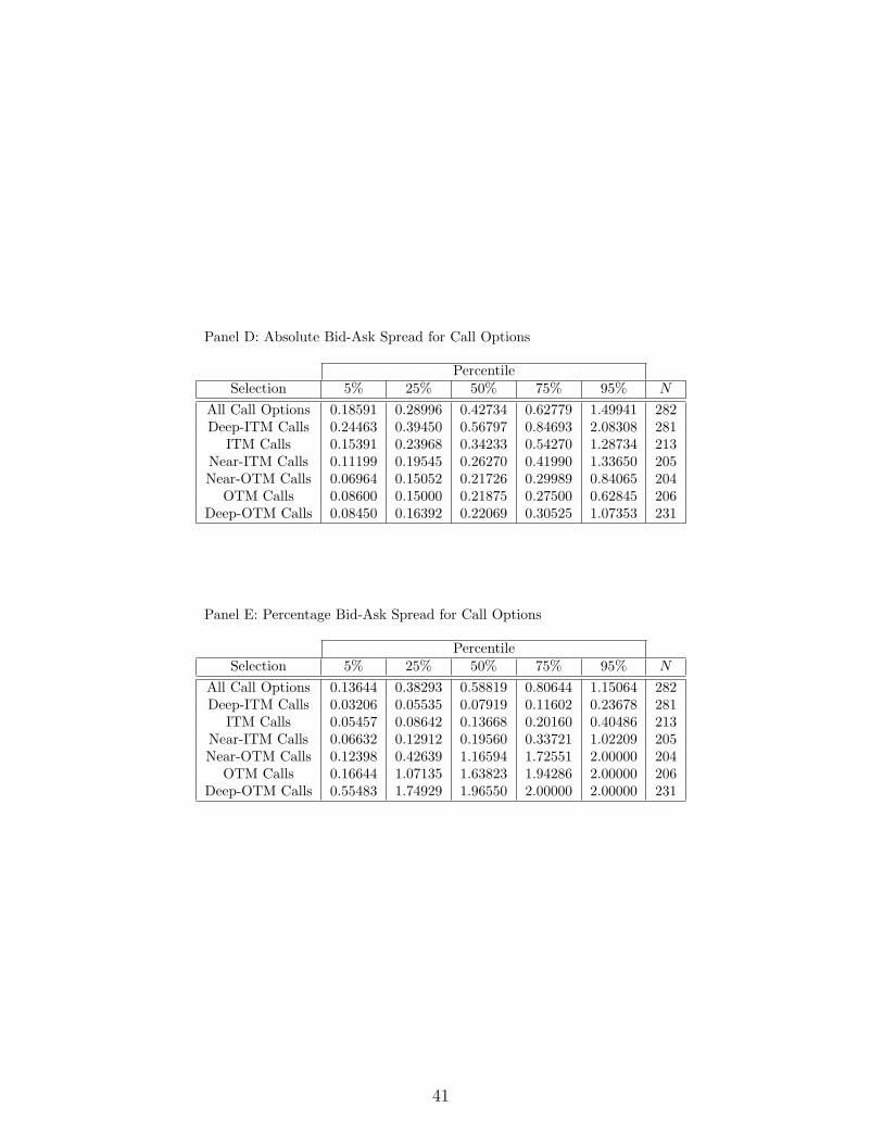
Table 4: Percentiles of Pricing Errors for Call Options on the Target Company

This table uses a sample of 282 cash mergers from 1996–2008, which have sufficiently liquid op-tions on the target company. The table compares the pricing errors for four models: our model,denoted by “MRB”; and three versions of the Black–Scholes formula, which differ only in theway the volatility is computed. Panel A reports the percentage error: for a given call optionon company i on day t, with strike price K and maturity T , the percentage error is defined asCi

model,K,T,t − CiK,T,t

/Ci

K,T,t

, depending on the model used. The MRB model defines the calloption price by Ci

K,T,t = qi(t) maxBi1−K, 0 e−r(T i

e−t) +(1− qi(t))CBS

(Bi2(t),K, r, T − t, σi

2), where:qi(t) is the estimated risk-neutral probability that the deal is successful; Bi

1 is the cash offer price;T i

e is the effective date of the deal; Bi2(t) is the fallback price, i.e., the price of company i if the

deal fails; σi2 is the estimated volatility of the fallback price Bi

2(t); and CBS

(S, K, r, T − t, σ) is theBlack–Scholes formula for the European call option price over a stock with price S at time t andvolatility σ. Under the three versions of the Black–Scholes formula, we define the option price byC

BS(Bi(t),K, r, T − t, σ), where Bi(t) is the stock price at t, and the volatility σ is defined as: (1)

the average implied volatility for at-the-money (ATM) call options quoted on company i duringthe time of the deal; (2) the implied volatility for an ATM call option quoted on the previous day(t − 1); (3) the implied volatility for a call option quoted on the previous day with the strike priceclosest to K. Panel B uses the absolute error:

Cimodel,K,T,t − Ci

K,T,t

. Panel C uses the absoluteerror divided by the bid-ask spread of the corresponding option. Once the error is computed foreach stock i, time t, and strike K, fix the stock i and compute the mean µi of the stock pricingerror over time and strike, equally weighted. The table reports various percentiles (5, 25, 50, 75,95) for µi over the 282 stocks in our sample. Each panel reports the results for: all call options;near-in-the-money (Near-ITM) calls, i.e., call options with the strike price K over the target stockprice Bt are in the range K/B ∈ [0.95, 1.0]; near-out-the-money (Near-OTM) calls with strike K sothat K/B ∈ [1.0, 1.05]; in-the-money (NTM) with K/B ∈ [0.90, 0.95]; out-the-money (ITM) withK/B ∈ [1.05, 1.10]; deep-in-the-money (Deep-ITM) with K/B < 0.90; and deep-out-of-the-money(Deep-OTM) with K/B > 1.10. Panels D and E report percentiles over the absolute and thepercentage bid-ask spread, respectively. In all panels, N represents the number of cross-sectionalobservations. The estimates in the model are calculated using only the option with the highestvolume each day.

37

Panel A: Percentage Errors for Four Option Pricing Models

PercentileSelection Model 5% 25% 50% 75% 95% N

MRB 0.08591 0.18146 0.26059 0.36489 0.56335 282All Call BS: σ = σi

ATM0.10578 0.19007 0.33019 0.48892 1.11483 282

Options BS: σ = σiATM ,t−1

0.09937 0.20711 0.34223 0.51132 1.17115 282BS: σ = σi

K,t−10.05724 0.11697 0.18189 0.28775 0.51272 282

Deep MRB 0.00441 0.00866 0.01504 0.02186 0.04860 281In-The-Money BS: σ = σi

ATM0.00490 0.01061 0.01647 0.02609 0.05725 281

Calls BS: σ = σiATM ,t−1

0.00512 0.01191 0.01799 0.02664 0.05705 281(K/B < 0.9) BS: σ = σi

K,t−10.00580 0.01190 0.01820 0.02707 0.05023 281

MRB 0.01033 0.02273 0.04254 0.07307 0.16680 213In-The-Money BS: σ = σi

ATM0.01410 0.03369 0.05908 0.11064 0.26527 213


0.01711 0.03569 0.05514 0.08447 0.22226 213(K/B ∈ [0.9, 0.95]) BS: σ = σi

K,t−10.01666 0.03244 0.05306 0.08650 0.19545 213

Near MRB 0.01883 0.04720 0.08036 0.14519 0.47372 205In-The-Money BS: σ = σi

ATM0.03429 0.07514 0.13361 0.24715 0.81787 205


0.03371 0.06185 0.10413 0.20543 0.84077 205(K/B ∈ [0.95, 1.0]) BS: σ = σi

K,t−10.02609 0.05932 0.11563 0.25139 1.02767 205

Near MRB 0.06724 0.19704 0.42291 0.87243 2.18229 204Out-The-Money BS: σ = σi

ATM0.11584 0.33458 0.62771 1.19446 5.14470 204


0.06646 0.20413 0.48669 0.85884 2.09441 204(K/B ∈ [1.0, 1.05]) BS: σ = σi

K,t−10.05744 0.19738 0.38476 0.68261 1.59153 204

MRB 0.12166 0.41035 0.67209 0.98636 1.41742 206Out-The-Money BS: σ = σi

ATM0.20219 0.53450 0.81586 1.21704 3.91596 206


0.10950 0.47117 0.85423 1.58244 6.21376 206(K/B ∈ [1.05, 1.10]) BS: σ = σi

K,t−10.06403 0.23956 0.41111 0.67903 1.78833 206

Deep MRB 0.37606 0.71212 0.94370 1.00000 1.44190 231Out-The-Money BS: σ = σi

ATM0.36172 0.80532 0.97943 1.00000 2.22103 231


0.35484 0.86320 1.00000 1.30257 4.27091 231(K/B > 1.1) BS: σ = σi

K,t−10.09207 0.23402 0.46254 0.68593 1.18797 231

38

Panel B: Absolute Errors for Four Option Pricing Models



ATM0.04276 0.07867 0.12097 0.22181 0.57306 282


0.04640 0.08307 0.12038 0.20428 0.52179 282BS: σ = σi

K,t−10.03718 0.07181 0.11111 0.17533 0.42242 282


ATM0.03071 0.06251 0.10534 0.17794 0.53655 281


0.03299 0.06943 0.10793 0.18433 0.51245 281(K/B < 0.9) BS: σ = σi

K,t−10.03605 0.07058 0.11032 0.18822 0.51498 281


ATM0.02794 0.09433 0.16740 0.33065 0.93220 213


0.03144 0.08530 0.14849 0.28918 0.69731 213(K/B ∈ [0.9, 0.95]) BS: σ = σi

K,t−10.04069 0.09344 0.14196 0.25583 0.52557 213


ATM0.03966 0.08944 0.18748 0.40083 1.27648 205


0.04046 0.08099 0.14916 0.29604 0.61143 205(K/B ∈ [0.95, 1.0]) BS: σ = σi

K,t−10.04053 0.09083 0.17234 0.34007 0.62459 205


ATM0.02674 0.07389 0.14563 0.38565 1.21321 204


0.02687 0.06036 0.11406 0.23950 0.70509 204(K/B ∈ [1.0, 1.05]) BS: σ = σi

K,t−10.02070 0.05155 0.09327 0.20685 0.56115 204


ATM0.03606 0.07438 0.13524 0.31414 1.04700 206


0.03733 0.07782 0.12686 0.28159 1.03029 206(K/B ∈ [1.05, 1.10]) BS: σ = σi

K,t−10.01630 0.04183 0.06996 0.12167 0.39998 206


ATM0.04280 0.08340 0.12500 0.24525 0.68421 231


0.03864 0.08744 0.13679 0.26473 0.77783 231(K/B > 1.1) BS: σ = σi

K,t−10.01156 0.02901 0.05474 0.10208 0.28423 231

39

Panel C: Absolute Errors Divided by Observed Bid-Ask Spread for Four Option Pricing Models



ATM0.18701 0.27737 0.40442 0.66493 1.65719 282


0.20566 0.32979 0.42908 0.63422 1.63183 282BS: σ = σi

K,t−10.17545 0.27418 0.35168 0.52383 1.03465 282


ATM0.07847 0.12118 0.20511 0.35230 0.79279 281


0.08840 0.14413 0.22661 0.37496 0.88582 281(K/B < 0.9) BS: σ = σi

K,t−10.09922 0.16045 0.22724 0.36447 0.70894 281


ATM0.09610 0.25648 0.52789 1.11088 2.66648 213


0.12387 0.26284 0.44932 0.91271 2.23472 213(K/B ∈ [0.9, 0.95]) BS: σ = σi

K,t−10.14098 0.28764 0.48538 0.79276 1.70762 213


ATM0.17202 0.38034 0.74865 1.49529 4.87438 205


0.16331 0.38419 0.58142 1.06230 2.47430 205(K/B ∈ [0.95, 1.0]) BS: σ = σi

K,t−10.15370 0.38680 0.65649 1.34888 3.44949 205


ATM0.21536 0.44726 0.80527 1.82159 5.58248 204


0.16095 0.36714 0.56192 1.07262 3.61276 204(K/B ∈ [1.0, 1.05]) BS: σ = σi

K,t−10.13582 0.32219 0.49326 0.85702 2.61802 204


ATM0.23385 0.44178 0.64746 1.54473 5.90195 206


0.22807 0.44571 0.71525 1.47772 6.87030 206(K/B ∈ [1.05, 1.10]) BS: σ = σi

K,t−10.08484 0.22005 0.38292 0.69955 1.78870 206


ATM0.29794 0.47649 0.50000 0.76486 2.46184 231


0.32090 0.49447 0.57293 0.90661 3.19430 231(K/B > 1.1) BS: σ = σi

K,t−10.05344 0.16482 0.29548 0.43982 0.96805 231

40

Panel D: Absolute Bid-Ask Spread for Call Options

PercentileSelection 5% 25% 50% 75% 95% N

All Call Options 0.18591 0.28996 0.42734 0.62779 1.49941 282Deep-ITM Calls 0.24463 0.39450 0.56797 0.84693 2.08308 281

ITM Calls 0.15391 0.23968 0.34233 0.54270 1.28734 213Near-ITM Calls 0.11199 0.19545 0.26270 0.41990 1.33650 205Near-OTM Calls 0.06964 0.15052 0.21726 0.29989 0.84065 204

OTM Calls 0.08600 0.15000 0.21875 0.27500 0.62845 206Deep-OTM Calls 0.08450 0.16392 0.22069 0.30525 1.07353 231

Panel E: Percentage Bid-Ask Spread for Call Options

PercentileSelection 5% 25% 50% 75% 95% N

All Call Options 0.13644 0.38293 0.58819 0.80644 1.15064 282Deep-ITM Calls 0.03206 0.05535 0.07919 0.11602 0.23678 281

ITM Calls 0.05457 0.08642 0.13668 0.20160 0.40486 213Near-ITM Calls 0.06632 0.12912 0.19560 0.33721 1.02209 205Near-OTM Calls 0.12398 0.42639 1.16594 1.72551 2.00000 204

OTM Calls 0.16644 1.07135 1.63823 1.94286 2.00000 206Deep-OTM Calls 0.55483 1.74929 1.96550 2.00000 2.00000 231

41

Table 5: The Call Price Kink and the Risk-Neutral Probability

This table uses a sample of 282 cash mergers from 1996–2008 with sufficiently liquid options onthe target company. Consider the call price kink multiplied by the time discont factor, Ckink =

er(T−t)

∂C∂K

K↓B1

−

∂C∂K

K↑B1

, which according to Equation (10) satisfies Ckink = q(t). The

table reports a pooled panel regression of the (natural) logarithm of the call price kink on thelogarithm of the estimated risk-neutral probability. T-statistics are reported in parentheses, and areobtained from standard errors clustered by firm.

OLS Regression of ln(Ckink) on ln(q)const ln(q) Adj. R2 No. of Obs.

ln(Ckink) −0.006 0.922∗∗∗ 21.56% 13,181(−0.05) (4.19)

42

Table 6: The Success Probability as a Predictor of Deal Outcome

This table uses a sample of 282 cash mergers from 1996–2008, which have sufficiently liquid optionson the target company. It compares the predictive power of the risk-neutral probability q estimatedusing our model with that estimated using a naive method. For each company i, consider 10 equallyspaced days tn throughout the deal: for each n = 1, . . . , 10, choose tn the closest integer strictlysmaller than nTe

10 . Use the model to compute qi(tn), the risk-neutral probability that the deal issuccessful. Define also qi(tn) using a “naive” method: qi

naive(tn) = Bi(tn)−Bi0

Bi1−Bi

0, where Bi(tn) is the

stock price at tn, Bi1 is the cash offer price, and Bi

0 is the stock price before the deal was announced.At each tn, compute perform a probit regression of outcome of deal i (1 if it succeeds, 0 if it fails) onthe success probability qi(tn). The figures reported in the table are the pseudo-R2. The estimatesin the model are calculated using only the option with the highest volume each day.

Pseudo-R2 of Probit Regression of Outcomeon the Success Probability Estimated at nTe

10

n R2 for q R2 for qnaive N

1 0.11678 0.00116 2792 0.11508 0.00311 2793 0.13040 0.01684 2794 0.20788 0.03757 2795 0.22979 0.03091 2796 0.29651 0.03250 2797 0.38594 0.04887 2798 0.43682 0.08845 2799 0.42681 0.14203 27910 0.47306 0.28219 279

43

Table 7: The Behavior of the Fallback Price after a Takeover Announcement

This table uses a sample of 282 cash mergers from 1996–2008, which have sufficiently liquid optionson the target company. For a company i subject to a takeover deal in our sample, it comparesthe fallback price Bi

2(tn), estimated using our model, with the stock price Bi0 before the deal an-

nouncement. The fallback price is estimated at 10 equally spaced days tn throughout the deal: foreach n = 1, . . . , 10, choose tn the closest integer strictly smaller than nTe

10 . The regression model isln(Bi

2(tn)) = a + b ln(Bi0) + ε. t-statistics are reported in parentheses. The estimates in the model

are calculated using only the option with the highest volume each day.

Regression of Log-Fallback Priceon Log-Price before Announcement

n a b R2 N

1 0.20846 0.97585 0.94556 279(4.658) (69.365)

2 0.24639 0.96766 0.94474 279(5.509) (68.818)

3 0.26334 0.96537 0.94552 279(5.946) (69.338)

4 0.25530 0.96815 0.93993 279(5.458) (65.834)

5 0.23855 0.97203 0.92547 279(4.525) (58.647)

6 0.21793 0.97876 0.91872 279(3.917) (55.954)

7 0.21081 0.98186 0.92124 279(3.842) (56.919)

8 0.22492 0.98073 0.92512 279(4.218) (58.500)

9 0.24132 0.97882 0.91444 279(4.217) (54.409)

10 0.27167 0.97273 0.90903 279(4.619) (52.613)

44

Date post:	12-Mar-2018
Category:	Documents
Upload:	hoangdien
View:	215 times
Download:	2 times

Option Prices and the Probability of Success of Cash … Prices and the Probability of Success of...

Documents