Option pricing in multivariate stochastic volatility models of OU type Johannes Muhle-Karbe * Oliver Pfaffel † Robert Stelzer ‡ We present a multivariate stochastic volatility model with leverage, which is flexible enough to recapture the individual dynamics as well as the interdependencies between several assets, while still being highly analytically tractable. First, we derive the characteristic function and give conditions that ensure its analyti- city and absolute integrability in some open complex strip around zero. Therefore we can use Fourier methods to compute the prices of multi-asset options efficiently. To show the applicability of our results, we propose a concrete specification, the OU-Wishart model, where the dynamics of each individual asset coincide with the popular Γ-OU BNS model. This model can be well calibrated to market prices, which we illustrate with an example using options on the exchange rates of some major currencies. Finally, we show that covariance swaps can also be priced in closed form. AMS Subject Classification 2000: Primary: 91B28, Secondary: 60G51 Keywords: multivariate stochastic volatility models, OU-type processes, option pricing 1. Introduction This paper deals with the pricing of options depending on several underlying assets. While there is a vast amount of literature on the pricing of single-asset options, see e.g. Cont and Tankov (2004) or Schoutens (2003) for an overview, the amount of literature considering the multi-asset case is rather limited. This is most likely due to the fact that the trade-off between flexibility and tractability is par- ticularly delicate in a multivariate setting. On the one hand, the model under consideration should be flexible enough to recapture stylized facts observed in real option prices. When dealing with multiple underlyings, this becomes challenging, since not only the individual assets but also their joint beha- viour has to be taken into account. On the other hand, one needs enough mathematical structure to * Departement f¨ ur Mathematik, ETH Z¨ urich, R¨ amistrasse 101 CH-8092 Z¨ urich. Email: [email protected]† TUM Institute for Advanced Study & Zentrum Mathematik, Technische Universit¨ at M¨ unchen, Parkring 13, D-85748 Garching, Germany. Email: [email protected]‡ Institute of Mathematical Finance, Ulm University, Helmholtzstraße 18, D-89081 Ulm, Germany. Email: [email protected]1
Transcript
Option pricing in multivariate stochasticvolatility models of OU type
Johannes Muhle-Karbe∗ Oliver Pfaffel† Robert Stelzer‡
We present a multivariate stochastic volatility model with leverage, which is flexibleenough to recapture the individual dynamics as well as the interdependencies betweenseveral assets, while still being highly analytically tractable.
First, we derive the characteristic function and give conditions that ensure its analyti-city and absolute integrability in some open complex strip around zero. Therefore we canuse Fourier methods to compute the prices of multi-asset options efficiently. To show theapplicability of our results, we propose a concrete specification, the OU-Wishart model,where the dynamics of each individual asset coincide with the popular Γ-OU BNS model.This model can be well calibrated to market prices, which we illustrate with an exampleusing options on the exchange rates of some major currencies. Finally, we show thatcovariance swaps can also be priced in closed form.
This paper deals with the pricing of options depending on several underlying assets. While there is avast amount of literature on the pricing of single-asset options, see e.g. Cont and Tankov (2004) orSchoutens (2003) for an overview, the amount of literature considering the multi-asset case is ratherlimited. This is most likely due to the fact that the trade-off between flexibility and tractability is par-ticularly delicate in a multivariate setting. On the one hand, the model under consideration should beflexible enough to recapture stylized facts observed in real option prices. When dealing with multipleunderlyings, this becomes challenging, since not only the individual assets but also their joint beha-viour has to be taken into account. On the other hand, one needs enough mathematical structure to∗Departement fur Mathematik, ETH Zurich, Ramistrasse 101 CH-8092 Zurich. Email:[email protected]
†TUM Institute for Advanced Study & Zentrum Mathematik, Technische Universitat Munchen, Parkring 13, D-85748Garching, Germany. Email: [email protected]
calculate option prices in the first place and to be able to calibrate the model to market prices. Dueto an increasing number of state variables and parameters, this is also not an easy task in a multidi-mensional framework. In this article we propose the multivariate OU-type stochastic volatility modelof Pigorsch and Stelzer (2009) in the generalised form introduced in Barndorff-Nielsen and Stelzer(2011), which seems to present a reasonable compromise between these competing requirements. Thelog-price processes Y = (Y 1, . . . ,Y d) of d financial assets are modelled as
dYt = (µ +β (Σt))dt +Σ12t dWt +ρ(dLt), (1.1)
dΣt = (AΣt +ΣtAT)dt +dLt , (1.2)
where µ ∈ Rd , A is a real d×d matrix, and β , ρ are linear operators from the real d×d matrices toRd . Moreover, W is an Rd-valued Wiener process and L is an independent matrix subordinator, i.e. aLevy process which only has positive semidefinite increments. Hence, the covariance process Σ is anOrnstein-Uhlenbeck (henceforth OU) type process with values in the positive semidefinite matrices,cf. Barndorff-Nielsen and Stelzer (2007). Thus we call (1.1), (1.2) the multivariate stochastic volatilitymodel of OU type. The positive semidefinite OU type process Σ introduces a stochastic volatility and,what is difficult to achieve using several univariate models, a stochastic correlation between the assets.Moreover, Σ is mean reverting and increases only by jumps. The jumps represent the arrival of newinformation that results in positive shocks in the volatility and positive or negative shocks in thecorrelation of some assets. Due to the leverage term ρ(dLt) they are correlated with price jumps. Thepresent model is a multivariate generalisation of the non-Gaussian OU type stochastic volatility modelintroduced by Barndorff-Nielsen and Shepard (2001) (henceforth BNS model). For one underlying,these models are found to be both flexible and tractable in Nicolato and Venardos (2003). The keyreason is that the characteristic function of the return process can often be computed in closed form,which allows European options to be be priced efficiently using the Fourier methods introduced byCarr and Madan (1999b) and Raible (2000). In the present study, we show that a similar approach isalso applicable in the multivariate case. Recently, Benth and Vos (2009) discussed a somewhat similarmodel in the context of energy markets. However, they do not establish conditions for the applicabilityof Fourier pricing and, more importantly, do not calibrate their model to market prices.
Alternatively, the covariance process Σ can also be modelled by other processes taking values in thepositive semidefinite matrices. In particular, several authors have advocated to use a diffusion modelbased on the Wishart process, cf., Da Fonseca, Grasselli and Tebaldi (2007), Gourieroux (2007),Gourieroux and Sufana (2010), Da Fonseca and Grasselli (2010), for instance. This leads to a mul-tivariate generalisation of the model of Heston (1993). However, there is empirical evidence suggest-ing that volatility jumps (together with the stock price), cf. Jacod and Todorov (2010), which cannotbe recaptured by a diffusion model. Moreover, the treatment of square-root processes on the cone ofpositive semidefinite matrices is mathematically quite involved, see Cuchiero, Filipovic, Mayerhoferand Teichmann (2010).1 For example, whereas Da Fonseca and Grasselli (2010) have very recentlysucceeded in calibrating their model to market prices, the resulting parameters do no satisfy the driftcondition for the existence of the underlying square-root diffusion, suggesting that a more sophistic-ated optimization routine is necessary.
Another possible approach is to consider multivariate models based on a concatenation of uni-variate building blocks. This approach is taken, e.g., by Luciano and Schoutens (2006) using Levy
1This study generalizes the theory of affine processes from the positive univariate factors treated in Duffie, Pan andSingleton (2000); Duffie, Filipovic and Schachermayer (2003) to stochastic factor processes taking values in the cone ofsymmetric positive semidefinite matrices. In particular, to ensure the existence of square-root processes, a quite intricatedrift condition turns out to be necessary.
2
1. Introduction
processes, by Dimitroff, Lorenz and Szimayer (2010), who consider a multivariate Heston model,and by Hubalek and Nicolato (2005), who put forward a multifactor BNS model. However, all thesemodels have either a somewhat limited capability to catch complex dependence structures (compareSection 4.2) or lead to tricky (factor) identification issues. Apart from models where all parameters aredetermined by single-asset options, we are not aware of successful calibrations of such models. Thepaper of Ma (2009) proposes a two-dimensional Black-Scholes model where the correlation betweenthe two Brownian motions is stochastic and given by a diffusion process with values in an intervalcontained in [−1,1]. However, pricing can only be done via Monte-Carlo simulation in this model. Inaddition, an extension to higher dimensions is not obvious, since the necessary positive semidefinite-ness of the correlation matrix of the Brownian noise imposes additional constraints, which are hard toincorporate.
The remainder of this paper is organised as follows. Sections 2.1 and 2.2 introduce the multivari-ate stochastic volatility model of OU type. Afterwards, we derive the joint characteristic function of(Yt ,Σt). We then show in Section 2.4 that a simple moment condition on L implies analyticity and ab-solute integrability of the moment generating function of Yt in some open complex strip around zero.Equivalent martingale measures are discussed in Section 2.5, where we also present a subclass thatpreserves the structure of our model. In Section 3, we recall how to use Fourier methods to computeprices of multi-asset options efficiently. Subsequently, we propose the OU-Wishart model, where L isa compound Poisson process with Wishart distributed jumps. It turns out that the OU-Wishart modelhas margins which are in distribution equivalent to a Γ-OU BNS model, one of the tractable specific-ations commonly used in the univariate case. Moreover, the characteristic function can be computedin closed form, which makes option pricing and calibration particularly feasible. In an illustrative ex-ample we calibrate a bivariate OU-Wishart model to market prices, and compare its performance tothe multivariate Variance Gamma model of Luciano and Schoutens (2006) and a multivariate exten-sion with stochastic volatility. As a final application, we show that covariance swaps can also be pricedin closed form in Section 5. The appendix contains a result on multidimensional analytic functionswhich is needed to establish the regularity of the moment generating function in Section 2.4.
Notation
Md,n(R) (resp. Md,n(C)) represent the d×n matrices with real (resp. complex) entries. We abbreviateMd(·) = Md,d(·). Sd denotes the subspace of Md(R) of all symmetric matrices. We write S+d for thecone of all positive semidefinite matrices, and S++
d for the open cone of all positive definite matrices.The identity matrix in Md(R) is denoted by Id . σ(A) denotes the set of all eigenvalues of A ∈Md(C).We write Re(z) and Im(z) for the real or imaginary part of z ∈ Cd or z ∈ Md(C), which has to beunderstood componentwise. The components of a vector or matrix are denoted by subscripts, howeverfor stochastic processes we use superscripts to avoid double indices.
On Rd , we typically use the Euclidean scalar product, 〈x,y〉Rd := xTy, and on Md(R) or Sd thescalar products given by 〈A,B〉Md(R) := tr(ATB) or 〈A,B〉Sd
:= tr(AB) respectively. However, due to theequivalence of all norms on finite dimensional vector spaces, most results here hold true independentlyof the norm. We also write 〈x,y〉 = xTy for x,y ∈ Cd , although this is only a bilinear form but not ascalar product on Cd .
We denote by vec : Md(R)→ Rd2the bijective linear operator that stacks the columns of a matrix
below one other. With the above norms, vec is a Hilbert space isometry. Likewise, for a symmetricmatrix S ∈ Sd we denote by vech(S) the vector consisting of the columns of the upper-diagonal partincluding the diagonal.
Furthermore, we employ an intuitive notation concerning integration with respect to matrix-valued
3
2. The multivariate stochastic volatility model of OU type
processes. For an Mm,n(R)-valued Levy process L, and Md,m(R) resp. Mn,p(R)- valued processes X ,Yintegrable with respect to L, the term
∫ t0 Xs dLsYs is to be understood as the d× p (random) matrix with
(i, j)-th entry ∑mk=1 ∑
nl=1∫ t
0 X iks dLkl
s Y l js .
2. The multivariate stochastic volatility model of OU type
For the remainder of the paper, fix a filtered probability space (Ω,F ,(Ft)t∈[0,T ],P) in the sense ofJacod and Shiryaev (2003, I.1.3), where F0 = Ω, /0 is trivial and T > 0 is a a fixed terminal time.
2.1. Positive semidefinite processes of OU type
To formulate our model, we need to introduce the concept of matrix subordinators as studied inBarndorff-Nielsen and Perez-Abreu (2008).
Definition 2.1. An Sd-valued Levy Process L = (Lt)t∈R+ is called matrix subordinator, if Lt−Ls ∈ S+dfor all t > s.
The characteristic function of a matrix subordinator L is given by E(eitr(ZL1)) = exp(ψL(Z)) for thecharacteristic exponent
ψL(Z) = itr(γLZ)+∫S+d(eitr(XZ)−1)κL(dX), Z ∈Md(R),
where γL ∈ S+d and κL is a Levy measure on Sd with κL(Sd\S+d ) = 0 and∫||X ||≤1 ||X || κL(dX)< ∞.
Positive semidefinite processes of OU type are a generalisation of nonnegative OU type processes(cf. Barndorff-Nielsen and Stelzer (2007)). Let L be a matrix subordinator and A ∈Md(R). The posit-ive semidefinite OU type process Σ=(Σt)t∈R+ is defined as the unique strong solution to the stochasticdifferential equation
dΣt = (AΣt +ΣtAT)dt +dLt , Σ0 ∈ S+d . (2.1)
It is given by
Σt = eAtΣ0eATt +
∫ t
0eA(t−s) dLs eAT(t−s). (2.2)
Since Σt ∈ S+d for all t ∈R+, this process can be used to model the stochastic evolution of a covariancematrix. As in the univariate case there exists a closed form expression for the integrated volatility.Suppose
0 /∈ σ(A)+σ(A). (2.3)
Then the integrated OU type process Σ+ is given by
Σ+t :=
∫ t
0Σs ds = A−1(Σt −Σ0−Lt), (2.4)
where A : X 7→ AX +XAT. Note that condition (2.3) implies that the operator A is invertible, cf. Hornand Johnson (1990, Theorem 4.4.5). In the case where Σ is mean reverting, i.e., A only has eigenvalueswith strictly negative real part, condition (2.3) is trivially satisfied.
4
2. The multivariate stochastic volatility model of OU type
2.2. Definition and marginal dynamics of the model
The following model was introduced and studied in Pigorsch and Stelzer (2009) from a statisticalpoint of view in the no-leverage case and has also been considered in Barndorff-Nielsen and Stelzer(2011). Here we discuss its applicability to option pricing.
Let L be a matrix subordinator with characteristic exponent ψL and W an independent Rd-valuedWiener process. The multivariate stochastic volatility model of OU type is then given by
with linear operators β ,ρ : Md(R)→ Rd , µ ∈ Rd , and A ∈Md(R) such that 0 /∈ σ(A)+σ(A).We have specified the risk premium β and the leverage operator ρ in a quite general form. The
following specification turns out to be particularly tractable.
Definition 2.2. We call β and ρ diagonal if, for β1, . . . ,βd ∈ R and ρ1, . . . ,ρd ∈ R,
β (X) =
β1X11...
βdXdd
, ρ(X) =
ρ1X11...
ρdXdd
, ∀X ∈Md(R).
In the following, we will denote for each i ∈ 1, . . . ,d by β i(X) and ρ i(X) the i-th componentof the vector β (X) or ρ(X) respectively. The marginal dynamics of the individual assets have beenderived in Barndorff-Nielsen and Stelzer (2011, Proposition 4.3).
Theorem 2.3. Let i ∈ 1, . . . ,d. Then we have
(Y i
t)
t∈R+
f idi=
(µit +β
i(Σ+t )+
∫ t
0(Σii
s )12 dW i
s +ρi(Lt)
)t∈R+
,
wheref idi= denotes equality of all finite dimensional distributions.
Let us now consider the case where A is a diagonal matrix, A =
(a1 0
. . .0 ad
), and β , ρ are diagonal
as well. Then, for every i ∈ 1, . . . ,d, we have
dY it
f idi= (µi +βiΣ
iit )dt +(Σii
t )12 dW i
t +ρi dLiit , (2.7)
dΣiit = 2aiΣ
iit dt +dLii
t . (2.8)
Evidently, every diagonal element Lii, i = 1, . . . ,d, of a matrix subordinator L is a univariate subor-dinator, and thus Σii is a nonnegative OU type process. Consequently, the model for the i-th asset isequivalent in distribution to a univariate BNS model.
2.3. Characteristic function
Let 〈·, ·〉V , 〈·, ·〉W be bilinear forms as introduced in the notation, where V ,W may be either Rd , Cd orMd(·). Given a linear operator T : V →W , the adjoint T ∗ : W →V is the unique linear operator suchthat 〈T x,y〉W = 〈x,T ∗y〉V for all x ∈V and y ∈W . Directly by definition we obtain the following
5
2. The multivariate stochastic volatility model of OU type
Lemma 2.4. Let y ∈ Rd , z ∈Md(R) and t ∈ R+. Then the adjoints of the linear operators
A : X 7→ AX +XAT, B(t) : X 7→ eAtXeATt −X ,
C (t) : X 7→ eAtXeATtz+β (A−1(B(t)X))yT+ρ(X)yT+i2
yyTA−1(B(t)X)
on Md(C) are given by
A∗ : X 7→ ATX +XA, B(t)∗ : X 7→ eATtXeAt −X ,
C (t)∗ : X 7→ eATtXzTeAt +ρ∗(Xy)+B(t)∗A−∗
(β∗(Xy)+
i2
XyyT).
Note that for diagonal ρ it holds that ρ∗(X) =
(ρ1X11 0
. . .0 ρdXdd
)for all X ∈Md(R).
Our main objective in this section is to compute the joint characteristic function of (Yt ,Σt). This willpave the way for Fourier pricing of multi-asset options later on. Note that we use the scalar product
〈(x1,y1),(x2,y2)〉 := xT1 x2 + tr(yT1 y2)
on Rd×Md(R).
Theorem 2.5 (Joint characteristic function). For every (y,z) ∈ Rd ×Md(R) and t ∈ R+, the jointcharacteristic function of (Yt ,Σt) is given by
E[exp(i〈(y,z),(Yt ,Σt)〉)] = exp
iyT(Y0 +µt)+ itr(Σ0eATtzeAt)
+itr(
Σ0
(eATtA−∗
(β∗(y)+
i2
yyT)
eAt −A−∗(
β∗(y)+
i2
yyT)))
+∫ t
0ψL
(eATszeAs +ρ
∗(y)+ eATsA−∗(
β∗(y)+
i2
yyT)
eAs−A−∗(
β∗(y)+
i2
yyT))
ds,
where A−∗ := (A∗)−1 denotes the inverse of the adjoint of A : X 7→ AX +XAT, that is, the inverse ofA∗ : X 7→ ATX +XA.
Note that for z = 0 we obtain the characteristic function of Yt .
Proof. Since Σ is adapted to the filtration generated by L, and by the independence of L and W ,
E[exp(〈(y,z),(Yt ,Σt)〉)] = eiyT(Y0+µt)E[
eitr(zTΣt)+iyT(β (Σ+t )+ρ(Lt))E
(eiyT
∫ t0 Σ
12s dWs
∣∣∣(Ls)s∈R+
)]= eiyT(Y0+µt)E
[eitr(zTΣt)+iyT(β (Σ+
t )+ρ(Lt)) exp(−1
2yTΣ
+t y)]
.
By (2.4) and using the fact that the trace is invariant under cyclic permutations the last term equals
eiyT(Y0+µt)E[eitr(zTΣt+β (A−1(Σt−Σ0−Lt))yT+ρ(Lt)yT+ i
2 yyTA−1(Σt−Σ0−Lt))].
In view of (2.2), we have
Σt −Σ0−Lt =∫ t
0B(t− s)dLs +B(t)Σ0,
6
2. The multivariate stochastic volatility model of OU type
for the linear operator B(t) from Lemma 2.4. Therefore
E[exp(i〈(y,z),(Yt ,Σt)〉]
=exp(
iyT(Y0 +µt)+ itr(
zTeAtΣ0eATt +β (A−1(B(t)Σ0))yT+
i2
yyTA−1(B(t)Σ0)
))× E
[exp(
itr(
zT∫ t
0eA(t−s) dLs eAT(t−s)+β
(A−1
(∫ t
0eA(t−s) dLs eAT(t−s)−Lt
))yT
+ρ(Lt)yT+i2
yyTA−1(∫ t
0eA(t−s) dLs eAT(t−s)−Lt
)))]=exp
(iyT(Y0 +µt)+ itr
(zTeAt
Σ0eATt +β (A−1(B(t)Σ0))yT+i2
yyTA−1(B(t)Σ0)
))× E
[exp
(itr
((∫ t
0C (t− s)dLs
)T
Id
))]
with the linear operator C (t) from Lemma 2.4, since A−1(∫ t
0 eA(t−s) dLs eAT(t−s)−Lt
)∈ Sd . An im-
mediate multivariate generalisation of results obtained in Rajput and Rosinski (1989, Proposition 2.4)(see also Eberlein and Raible (1999, Lemma 3.1)) yields an explicit formula for the expectation above:
E
[exp
(itr
((∫ t
0C (t− s)dLs
)T
Id
))]= exp
(∫ t
0ψL (C (s)∗Id) ds
).
By Lemma 2.4 we have
e∫ t
0 ψL(C (s)∗Id)ds = e∫ t
0 ψL
(eATszTeAs+ρ∗(y)+eATsA−∗(β ∗(y)+ i
2 yyT)eAs−A−∗(β ∗(y)+ i2 yyT)
)ds.
This expression is well-defined, because
eATszTeAs +ρ∗(y)+ eATsA−∗
(β∗(y)+
i2
yyT)
eAs−A−∗(
β∗(y)+
i2
yyT)∈Md(R)+ iS+d ,
for all s ∈ [0, t]. Indeed, this follows from
eATsA−∗(
yyT)
eAs−A−∗(
yyT)=∫ s
0eATuyyTeAu du ∈ S+d . (2.9)
Finally, we infer from Lemma 2.4 that
tr(
β (A−1(B(t)Σ0))yT+i2
yyTA−1(B(t)Σ0)
)= tr
(Σ0
(B(t)∗A−∗
(β∗(y)+
i2
yyT)))
,
which gives the desired result by noting that tr(zΣt) = tr(zTΣt).
2.4. Regularity of the moment generating function
In this section we provide conditions ensuring that the characteristic function of Yt admits an ana-lytic extension ΦYt to some open convex neighbourhood of 0 in Cd . Afterwards, we show absoluteintegrability. The regularity results obtained in this section will allow us to apply Fourier methods inSection 3 to compute option prices efficiently.
7
2. The multivariate stochastic volatility model of OU type
Definition 2.6. For any t ∈ [0,T ], the moment generating function of Yt is defined as
ΦYt (y) := E[exp(yTYt)],
for all y ∈ Cd such that the expectation exists.
Note that ΦYt may not exist anywhere but on iRd , where it coincides with the characteristic functionof Yt . The next lemma is a first step towards conditions for the existence and analyticity of the momentgenerating function ΦYt in a complex neighbourhood of zero.
Lemma 2.7. Let L be a matrix subordinator with cumulant transform ΘL, that is
ΘL(Z) = ψL(−iZ) = tr(γLZ)+∫S+d(etr(XZ)−1)κL(dX), Z ∈Md(C),
and let ε > 0. Then ΘL is analytic on the open convex set
Sε := Z ∈Md(C) : ||Re(Z)||< ε−S+d , (2.10)
if and only if ∫||X ||≥1
etr(RX)κL(dX)< ∞ for all R ∈Md(R) with ||R||< ε. (2.11)
Proof. If (2.11) holds, Duffie et al. (2003, Lemma A.2) implies that Z 7→ E(etr(ZL1)) = eΘL(Z) is ana-lytic on Sε . Due to Assumption (2.11), dominated convergence yields that ΘL is continuous on Sε .The claim now follows from Lemma A.1. Conversely, if ΘL is analytic on Sε , then Duffie et al. (2003,Lemma A.4) implies that E(tr(ZL1)) = eΘL(Z) for all Z ∈ Sε . Thus, by Sato (1999, Theorem 25.17),Condition (2.11) holds.
The next theorem is a nontrivial (especially due to the involved heavy matrix calculus) general-ization of Nicolato and Venardos (2003, Theorem 2.2) to the multivariate case. It holds for all sub-multiplicative matrix norms on Md(R) that satisfy
∣∣∣∣yyT∣∣∣∣ = ||y||2 for all y ∈ Rd , where we use the
Euclidean norm on Rd . For example, this holds true for the Frobenius and the spectral norm (theoperator norm associated to the Euclidean norm).
Theorem 2.8 (Strip of analyticity). Suppose the matrix subordinator L satisfies∫||X ||≥1
etr(RX)κL(dX)< ∞ for all R ∈Md(R) with ||R||< ε, (2.12)
for some ε > 0. Then the moment generating function ΦYt of Yt is analytic on the open convex set
Sθ := y ∈ Cd : ||Re(y)||< θ,
where
θ :=− ||ρ||(e2||A||t +1) ||A−1||
− ||β ||+√
∆ > 0 (2.13)
with
∆ :=(
||ρ||(e2||A||t +1) ||A−1||
+ ||β ||)2
+2ε
(e2||A||t +1) ||A−1||.
Moreover,
ΦYt (y) = exp(
yT(Y0 +µt)+ tr(Σ0Hy(t))+∫ t
0ΘL (Hy(s)+ρ
∗(y)) ds)
(2.14)
8
2. The multivariate stochastic volatility model of OU type
for all y ∈ Sθ , where
Hy(s) := eATsA−∗(
β∗(y)+
12
yyT)
eAs−A−∗(
β∗(y)+
12
yyT). (2.15)
Proof. The main part of the proof is to show that the function
G(y) := exp(
yT(Y0 +µt)+ tr(Σ0Hy(t))+∫ t
0ΘL (Hy(s)+ρ
∗(y)) ds)
is analytic on Sθ . First we want to find a θ such that for all u ∈ Rd with ||u|| < θ , it holds that||Hu(s)+ρ∗(u)||< ε for all s ∈ [0, t]. Since
The positive one is given by θ as stated in (2.13). Note that θ > 0, because p is a cup-shaped parabolawith p(0) =−ε < 0.
Now let y ∈ Sθ , i.e. y = u+ iv with ||u||< θ . Using Re(yyT) = uuT− vvT and (2.9) we get
Re(Hy(s)+ρ∗(y)) = Hu(s)+ρ
∗(u)− 12
(eATsA−∗(vvT)eAs−A−∗(vvT)
)= Hu(s)+ρ
∗(u)− 12
∫ s
0eATrvvTeAr dr.
Because of∫ s
0 eATrvvTeAr dr ∈ S+d , we have∫||X ||≥1
etr(Re(Hy(s)+ρ∗(y))X)κL(dX) =
∫||X ||≥1
etr((Hu(s)+ρ∗(u))X)e−12 tr((∫ s
0 eATrvvTeAr dr)
X)
κL(dX)< ∞
by Assumption (2.12), since ||Hu(s)+ρ∗(u)||< ε . Thus, by Lemma 2.7 the function
Sθ ∈ y 7→ΘL(Hy(s)+ρ∗(y))
is analytic on Sθ for every s ∈ [0, t]. An application of Fubini’s and Morera’s theorem shows thatintegration over [0, t] preserves analyticity, cf. Konigsberger (2004, p. 228), hence G is analytic on Sθ .Obviously, we have ΦYt (iy) = G(iy) for all y ∈ Rd by Theorem 2.5 and the definition of G. Thus,Duffie et al. (2003, Lemma A.4) finally implies ΦYt ≡ G on Sθ .
With Theorem 2.8 at hand, we can establish the following result:
Theorem 2.9 (Absolute integrability). If (2.12) holds for some ε > 0, the mapping w 7→ ΦYt (y+ iw)is absolutely integrable, for all y ∈ Rd with ||y||< θ , where θ is given as in Theorem 2.8.
9
2. The multivariate stochastic volatility model of OU type
Proof. As in the proof of Theorem 2.8, we obtain from
Re(Hy+iw(s)) = Hy(s)−12
∫ s
0eATswwTeAs ds
and Re(etr(Z))≤ |etr(Z)|= eRe(tr(Z)) = etr(Re(Z)) for Z ∈Md(C), that
Re(∫ t
0
∫S+d
(etr((Hy+iw(s)+ρ∗(y+iw))X)−1
)κL(dX)ds
)≤∫ t
0
∫S+d
(etr((Hy(s)+ρ∗(y))X)−1
)κL(dX)ds.
Using this inequality yields
|ΦYt (y+ iw)| ≤ΦYt (y)e− 1
2 tr(Σ0(eATt A−∗(wwT)eAt−A−∗(wwT)))− 12∫ t
0 tr(γL(eATsA−∗(wwT)eAs−A−∗(wwT)))ds
= ΦYt (y)e− 1
2〈(A−1B(t)(Σ0)+∫ t
0 A−1B(s)(γL)ds)w,w〉
with B(t) as in Lemma 2.4. Note that A−1B(t)(Σ0)+∫ t
where L is a driftless matrix subordinator with Levy measure κL. Clearly, this is our multivariatestochastic volatility model of OU type (2.5), (2.6), except that µ in (2.5) is replaced by µ − ρ(γL),such that there is no deterministic drift from the leverage term ρ(dLt).
In mathematical finance, Y is used to model the joint dynamics of the log-returns of d assets withprice processes Si
t = Si0eY i
t , where we set Y i0 = 0 from now on and, hence, S0 denotes the vector of
initial prices.The martingale property of the discounted stock prices (e−rtSt)t∈[0,T ] for a constant interest rate
r > 0 can be characterised as follows.
Theorem 2.10. The discounted price process (e−rtSt)t∈[0,T ] is a martingale if and only if, for i =1, . . . ,d, ∫
||X ||>1eρ i(X)
κL(dX)< ∞, (2.18)
and
βi(X) =−1
2Xii, X ∈ S+d , (2.19)
µi = r−∫S+d(eρ i(X)−1)κL(dX). (2.20)
10
2. The multivariate stochastic volatility model of OU type
Proof. Define St := e−rtSt for all t ∈ [0,T ] and let i ∈ 1, . . . ,d. By Ito’s formula and Jacod andShiryaev (2003, III.6.35), S i is a local martingale if and only if (2.18), (2.19) and (2.20) hold. Thus itremains to show that it is actually a true martingale under the stated assumptions. Since S is a positivelocal martingale, it is a supermartingale and hence a martingale if and only if E(S i
T ) = S i0 for all
i ∈ 1, . . . ,d. This can be seen as follows. By Theorem 2.3, (2.19) and (2.20) we have
E(S iT ) = S i
0E(
exp((µ i− r)T +β
i(Σ+T )+
∫ T
0(Σii
s )12 dW i
s +ρi(LT )
))= S i
0e−T
∫S+d
(eρi(X)−1)κL(dX)E(
e−12 (Σ
+T )
ii+ρ i(LT )E(
e∫ T
0 (Σiis )
12 dW i
s
∣∣∣∣(Ls)s∈[0,T ]
))= S i
0e−T
∫S+d
(eρi(X)−1)κL(dX)E(
eρ i(LT ))
= S i0.
This proves the assertion.
As in Nicolato and Venardos (2003, Theorem 3.1), it is possible to characterise the set of all equi-valent martingale measures (henceforth EMMs), if the underlying filtration is generated by W andL. More specifically, it follows from the Martingale Representation Theorem (cf. Jacod and Shiryaev(2003, III.4.34)), that the density process Zt = E(dQ
dP |Ft) of any equivalent martingale measure Q canbe written as
Z = E
(∫ ·0
ψsdWs +(Y −1)∗ (µL−νL)
)(2.21)
for suitable processes ψ and Y in this case. Here µL resp. νL denote the random measure of jumpsresp. its compensator (cf. Jacod and Shiryaev (2003, II.1) for more details). Under an arbitrary EMM,L may not be a Levy process, and W and L may not be independent. However, there is a subclass ofstructure preserving EMMs under which L remains a Levy process independent of W . This translatesinto the following specifications of ψ and Y (cf. Nicolato and Venardos (2003, Theorem 3.2) for theunivariate case):
Theorem 2.11 (Structure preserving EMMs). Let y : S+d → (0,∞) such that
(i)∫S+d(√
y(X)−1)2 κL(dX)< ∞,
(ii)∫||X ||>1 eρ i(X) κ
yL(dX)< ∞, i = 1, . . . ,d,
where κyL(B) :=
∫B y(X)κL(dX) for B ∈B(S+d ). Define the Rd-valued process (ψt)t∈[0,T ] as
ψt =−Σ− 1
2t
µ +β (Σt)+12
Σ11t...
Σddt
+
∫S+d(eρ1(X)−1)κ
yL(dX)
...∫S+d(eρd(X)−1)κ
yL(dX)
−1r
,
where 1 = (1, . . . ,1)T ∈Rd . Then Z = E (∫ ·
0 ψsdWs+(y−1)∗ (µL−νL)) is a density process, and theprobability measure Q defined by dQ
dP =ZT is an equivalent martingale measure. Moreover, W Q :=W−∫ ·0 ψsds is a Q-standard Brownian motion, and L is an independent driftless Q-matrix subordinator
with Levy measure κyL. The Q-dynamics of (Y,Σ) are given by
dY it =
(r−
∫S+d(eρ i(X)−1)κ
yL(dX)− 1
2Σ
iit
)dt +
(Σ
12t dW Q
t
)i
+ρi(dLt), i = 1, . . . ,d,
dΣt = (γL +AΣt +ΣtAT)dt +dLt .
11
3. Option pricing using integral transform methods
Proof. Since y−1 > −1, Z is strictly positive by Jacod and Shiryaev (2003, I.4.61). The martingaleproperty of Z follows along the lines of the proof of Nicolato and Venardos (2003, Theorem 3.2). Theremaining assertions follow from Kallsen (2006, Proposition 1) and the Levy-Khintchine formula byapplying the Girsanov-Jacod-Memin Theorem as in Kallsen (2006, Proposition 4) to the R 1
2 d(d+1)-valued process
L =
(W Q
0
)+vech(L),
where W Q :=W −∫ ·
0 ψsds.
The previous theorem shows that it is possible to use a model of the same type under the real-world probability measure P and some EMM Q, e.g. to do option pricing and risk management withinthe same model class. The model parameters under Q can be determined by calibration, the modelparameters under P by statistical methods.
3. Option pricing using integral transform methods
In this section we first recall results of Eberlein, Glau and Papapantoleon (2009) on Fourier pricing ingeneral multivariate semimartingale models. To this end, let S = (S1
0eY 1, . . . ,Sd
0eY d) be a d-dimensional
semimartingale such that the discounted price process (e−rtSt)t∈[0,T ] is a martingale under some pri-cing measure Q, for some constant instantaneous interest rate r > 0.
We want to determine the price EQ(e−rT f (YT − s)) of a European option with payoff f (YT − s) atmaturity T , where f : Rd → R+ is a measurable function and s := (− log(S1
0), . . . ,− log(Sd0)). Denote
by f the Fourier transform of f . The following theorem is from Eberlein et al. (2009, Theorem 3.2) andrepresents a multivariate generalisation of integral transform methods first introduced in the contextof option pricing by Carr and Madan (1999b) and Raible (2000).
Theorem 3.1 (Fourier Pricing). Fix R ∈ Rd , let g(x) := e−〈R,x〉 f (x) for x ∈ Rd , and assume that
(i) g ∈ L1∩L∞, (ii) ΦYT (R)< ∞, (iii) w 7→ΦYT (R+ iw) belongs to L1.
Then,
EQ(e−rT f (YT − s)) =e−〈R,s〉−rT
(2π)d
∫Rd
e−i〈u,s〉ΦYT (R+ iu) f (iR−u)du. (3.1)
Observe that Theorems 2.8 and 2.9 show that Conditions (ii) and (iii) are satisfied for our multivari-ate stochastic volatility model of OU type (2.5), (2.6) if condition (2.12) holds, i.e., if L has enoughexponential moments. More specifically, the vector R has to lie in the intersection of the domains ofΦYT and f .
We now present some examples. As is well-known, the Fourier transform of the payoff function ofa plain vanilla call option with strike K > 0, f (x) = (ex−K)+ is given by
f (z) =K1+iz
iz(1+ iz)(3.2)
for z ∈ C with Im(z) > 1. The Fourier transforms of many other single-asset options like barrier,self-quanto and power options as well as multi-asset options like worst-of and best-of options can befound, e.g., in the survey Eberlein et al. (2009). From the unpublished paper of Hubalek and Nicolato(2005) we have the following formulae for basket and spread options.
12
3. Option pricing using integral transform methods
Example 3.1. (i) The Fourier transform of f (x) = (K−∑dj=1 ex j)+, K > 0, that is the payoff func-
tion of a basket put option, is given by
f (z) = K1+i∑dj=1 z j
∏dj=1 Γ(iz j)
Γ(2+ i∑dj=1 z j)
for all z ∈ Cd with Im(z j) < 0, j = 1, . . . ,d. The price of the corresponding call can easily bederived using the put-call-parity (K− x)+ = (x−K)+− x+K. Since we have separated theinitial values s in (3.1), we can use FFT methods to compute the prices of weighted baskets forseveral weights efficiently.
(ii) The Fourier transform of the payoff function of a spread call option, f (x) = (ex1 − ex2 −K)+,K > 0, is given by
f (z) =K1+iz1+iz2
iz1(1+ iz1)
Γ(iz2)Γ(−iz1− iz2−1)Γ(−iz1−1)
for all z ∈C2 with Im(z1)> 1, Im(z2)< 0 and Im(z1+ z2)> 1, see also Hurd and Zhou (2010).
Since the Fourier transform of (ex1− ex2)+ does not exist anywhere, we cannot use Theorem 3.1 toprice zero-strike spread options. Nevertheless, we can derive a similar formula directly. Alternatively,one could use the change of numeraire technique of Margrabe (1978), which would lead to formulaeof a similar complexity.
Proposition 3.2 (Spread options with zero strike). Suppose that
Φ(Y 1T ,Y
2T )(R,1−R)< ∞ for some R > 1.
Then the price of a zero-strike spread option with payoff (S10eY 1
T −S20eY 2
T )+ is given by
EQ(e−rT (S1T −S2
T )+) =
eR(s2−s1)−s2−rT
2π
∫R
eiu(s2−s1)Φ(Y 1
T ,Y2T )(R+ iu,1−R− iu)
(R+ iu)(R+ iu−1)du,
where s1 =− ln(S10) and s2 =− ln(S2
0).
Observe that unlike for K > 0, one only has to compute a one-dimensional integral to determine theprice of a zero-strike spread option. This will be exploited in the calibration procedure in Section 4.
Proof. Let R > 1 and define fK(x) = (ex−K)+ for K > 0, and gK(x) = e−Rx fK(x). By Fourier inver-sion and (3.2) we have
fey(x) =1
2π
∫R
e(R+iu)xe(1−R−iu)y
(R+ iu)(R+ iu−1)du,
for all y ∈ R. Hence, for the function hey(x) := (S10ex−S2
0ey)+ = fey−s2 (x− s1) we get
hey(x) =1
2πeR(s2−s1)−s2
∫R
eiu(s2−s1)e(R+iu)xe(1−R−iu)y
(R+ iu)(R+ iu−1)du.
Finally, by Fubini’s theorem
EQ(heY 2T(Y 1
T )) =eR(s2−s1)−s2
2π
∫R2
∫R
eiu(s2−s1)e(R+iu)xe(1−R−iu)y
(R+ iu)(R+ iu−1)duP(Y 1
T ,Y2T )(dx,dy)
=eR(s2−s1)−s2
2π
∫R
eiu(s2−s1)Φ(Y 1
T ,Y2T )(R+ iu,1−R− iu)
(R+ iu)(R+ iu−1)du,
13
4. Calibration of the OU-Wishart model
where the application of Fubini’s theorem is justified by∫R2
∫R
∣∣∣ e(R+iu)xe(1−R−iu)y
(R+ iu)(R+ iu−1)
∣∣∣duP(Y 1T ,Y
2T )(dx,dy) =
∫R2
eRxe(1−R)y∫R|g1(u)|duP(Y 1
T ,Y2T )(dx,dy)
≤ ||g1||L1 Φ(Y 1T ,Y
2T )(R,1−R)< ∞,
since ||g1||L1 < ∞ as shown in Eberlein et al. (2009, Example 5.1).
4. Calibration of the OU-Wishart model
We now put forward a specific parametric specification of the model discussed in Section 2. To thisend, let n ∈ N, Θ ∈ S+d and let X be a d× n random matrix with i.i.d. standard normal entries. Thenthe matrix M := Θ
12 XXTΘ
12 is said to be Wishart distributed, written M ∼ Wd(n,Θ). Note that this
definition can be extended to noninteger n > d−1 using the characteristic function
Z 7→ det(Id−2iZΘ)−12 n, (4.1)
see Gupta and Nagar (2000, Theorem 3.3.7). Since M ∈ S+d almost surely, we can define a compoundPoisson matrix subordinator L with intensity λ and Wd(n,Θ) distributed jumps. We call the resultingmultivariate stochastic volatility model of OU type OU-Wishart model.
Remark 4.1. There exists a subclass of structure preserving EMMs Q (cf. Theorem 2.11) such that wehave an OU-Wishart model under both P and Q. This means that L is a compound Poisson process withWd(n,Θ) distributed jumps and intensity λ under P, and Wd(n,Θ) distributed jumps with intensity λ
under Q. We only need to assume that the Wishart distribution under both P and Q has a Lebesguedensity, i.e. n, n> d−1 and Θ,Θ∈ S++
d . Then one simply has to take y as the quotient of the accordingLevy densities. Hence, by Gupta and Nagar (2000, 3.2.1), y has to be defined as
y(X) =λ
λ
(2
12 (n−n)d Γd
(12 n)
Γd(1
2 n) det(Θ)
12 n
det(Θ)12 n
)−1
det(X)12 (n−n)e−
12 tr((Θ−1−Θ−1)X), X ∈ S+d .
Since we have∫S+d
etr(RX) κL(dX) = λ det(Id−2RΘ)−12 n by (4.1), we see that the compound Poisson
process L has exponential moments as long as ||R|| < 12||Θ|| , where ||·|| denotes the spectral norm.
Consequently, (2.12) holds for ε := 12||Θ|| , and we can apply the integral transform methods from the
previous section to compute prices of multi-asset options.Note that for the particularly simple special case of diagonal A, β and ρ , each asset follows a
BNS model at the margins by (2.7) and (2.8). In particular, for n = 2 we see that Lii, i = 1, . . . ,d, is acompound Poisson subordinator with exponentially distributed jumps, thus we have in distribution theΓ-OU BNS model with stationary Gamma distribution at the margins, cf., e.g., Nicolato and Venardos(2003, Section 2.2). Then, the characteristic functions of the single assets are known in closed form.Note that while the characteristic function of the stationary distribution of the marginal OU typeprocess is still known for n 6= 2, it no longer corresponds to a Gamma distribution in this case.
4.1. The OU-Wishart model in dimension 2
We work directly under a pricing measure Q and consider the following specific two-dimensional caseof our model, where we restrict ourselves in particular to a diagonal mean-reversion matrix A and a
14
4. Calibration of the OU-Wishart model
leverage term ρ such that both jumps of the respective variance and of the covariance enter the price.Our model is given by(
dY 1t
dY 2t
)=
((µ1µ2
)− 1
2
(Σ11
tΣ22
t
))dt +
(Σ11
t Σ12t
Σ12t Σ22
t
) 12(
dW 1t
dW 2t
)+
(ρ1 dL11
t +ρ12 dL12t
ρ2 dL22t +ρ21 dL12
t
)(
dΣ11t dΣ12
tdΣ12
t dΣ22t
)=
((γ1 00 γ2
)+
(2a1Σ11
t (a1 +a2)Σ12t
(a1 +a2)Σ12t 2a2Σ22
t
))dt +
(dL11
t dL12t
dL12t dL22
t
)with initial values
Y0 =
(00
), Σ0 =
(Σ11
0 Σ120
Σ120 Σ22
0
)∈ S++
2 ,
and parameters γ1,γ2 ≥ 0, a1,a2 < 0, ρ1,ρ2,ρ12,ρ21 ∈ R. L is a compound Poisson process with in-tensity λ and W2(n,Θ)-jumps, where n = 2 and
Θ =
(Θ11 Θ12Θ12 Θ22
)∈ S+2 .
Therefore all components of L jump at the same time. Since the second order properties of the Wis-hart distribution are known explicitly, cf. Gupta and Nagar (2000, Theorem 3.3.15), the conditionalcovariances of the jumps are given by
Cov(∆L11t ,∆L12
t |∆L11t 6= 0) = 4Θ11Θ12,
Cov(∆L22t ,∆L12
t |∆L11t 6= 0) = 4Θ22Θ12,
Cov(∆L11t ,∆L22
t |∆L11t 6= 0) = 4Θ
212.
This shows that even if ρ is diagonal, i.e., ρ12 = 0 = ρ21, the leverage terms of both assets are correl-ated. If ρ is non-diagonal, then the parameter θ12 also has an influence on the marginal distribution ofeach asset.
Multi-asset option pricing By (2.14) and (4.1), the joint moment generating function of (Y 1,Y 2)is given by
E[eyTYt ] = exp(
yTµt + tr(Σ0Hy(t))+∫ t
0tr(γLHy(s))ds+λ
∫ t
0
1det(I2−2(Hy(s)+ρ∗(y))Θ)
ds−λ t)
with Hy as in (2.15), A =(
a1 00 a2
), γL =
(γ1 00 γ2
)and ρ∗(y) =
(ρ1y1 ρ12y1ρ21y2 ρ2y2
). It does not seem to be
possible to obtain a closed form expression in terms of ordinary functions, unless one sets a1 = a2 =: a.
In this case, if ∆ =√
4b0b2−b21 6= 0, one has
E[ey1Y 1t +y2Y 2
t ] =exp
y1µ1t + y2µ2t +e2at −1
4atr(
Σ0
(y2
1− y1 y1y2y1y2 y2
2− y2
))+
14a
(γ1(y2
1− y1)+ γ2(y22− y2)
)( 12a
(e2at −1)− t)
+λ
2ab0
[b1
∆
(arctan
(2b2 +b1
∆
)− arctan
(2b2e2at +b1
∆
))+
12
ln(
b0 +b1 +b2
b2e4at +b1e2at +b0
)]+
λ
b0t−λ t
15
4. Calibration of the OU-Wishart model
with coefficients
b0 := 1+4det(B−C)+2tr(B−C),
b1 :=−8det(B)+4tr(B)tr(C)−4tr(BC)−2tr(B),
b2 := 4det(B),
∆ :=√
4b0b2−b21,
and matrices
B :=14a
(y2
1− y1 y1y2y1y2 y2
2− y2
)Θ, C :=
(ρ1y1 ρ12y1ρ21y2 ρ2y2
)Θ.
Note that arctan has to be understood as a function of complex argument to cover the case where theterm in the square root of ∆ is negative. If ∆ = 0, we obtain
E[ey1Y 1t +y2Y 2
t ] =exp
y1µ1t + y2µ2t +e2at −1
4atr(
Σ0
(y2
1− y1 y1y2y1y2 y2
2− y2
))+
14a
(γ1(y2
1− y1)+ γ2(y22− y2)
)( 12a
(e2at −1)− t)
+λ
2ab0
[b1
2b2e2at +b1− b1
2b2 +b1+
12
ln(
b0 +b1 +b2
b2e4at +b1e2at +b0
)]+
λ
b0t−λ t
.
Using det(A+B) = det(A)+det(B)+ tr(A)tr(B)− tr(AB) for A,B∈M2(R), the above formulae followfrom
and straightforward integration. Likewise, one can also derive a closed form expression for n= 4,6, . . .using Gradshteyn and Ryzhik (2007, 2.18(4)).
Consequently, one faces a tradeoff at this point. One possibility is to retain the flexibility of differentmean reversion speeds ai by evaluating the remaining integral using numerical integration. Alternat-ively, one can restrict attention to identical mean reversion speeds in order to have a closed-formexpression of the moment generating function at hand. The impact of this decision on the calibrationperformance is discussed in Section 4.2 below.
Single-asset option pricing For pricing single-asset options, one only needs the transforms ofthe marginal models, such that the above expressions simplify considerably. For example, the momentgenerating function of Y 1 is given by
E[ey1Y 1t ] = exp
y1µ
1t +e2a1t −1
4a1(y2
1− y1)Σ110 +
14a1
(1
2a1(e2a1t −1)− t
)(y2
1− y1)γ11L
+λ
2a1b0ln(
b0 +b1
b0 + e2a1tb1
)+
λ tb0−λ t
,
where b0 and b1 simplify to
b0 = 1+(
12a1
(y21− y1)−2ρ1y1
)Θ11−2ρ12y1Θ12,
b1 =−1
2a1(y2
1− y1)Θ11.
16
4. Calibration of the OU-Wishart model
Note that one can use the recursion formula stated in Gradshteyn and Ryzhik (2007, 2.155) to obtain aclosed form expression for W2(n,Θ)-jumps with n ∈ 2N, too. In the special case where the operator ρ
is diagonal, i.e., if ρ12 = ρ21 = 0, the margins are (in distribution) Γ-OU BNS models, whose momentgenerating function has been derived in Nicolato and Venardos (2003, Table 2.1).
Remark 4.2 (High Dimensionality). The above model can also be defined for d > 2, but of course,the Fourier formula (3.1) becomes numerically infeasible in high dimensions. Nevertheless, if ρ isdiagonal, the calibration of a high dimensional OU-Wishart model is still possible by only evaluatingoptions on two underlyings. Using zero strike spread options and provided the characteristic functionis known explicitly, this means that one only has to evaluate single integrals numerically, as in theunivariate case. Indeed, combining Barndorff-Nielsen and Stelzer (2011, Proposition 4.5) and thefact that every symmetric sub-matrix of a Wishart distributed matrix is again Wishart distributed, cf.Gupta and Nagar (2000, Theorem 3.3.10), it follows that the joint dynamics of each pair of assetsfollows a 2-dimensional OU-Wishart model as above. Hence, we can calibrate the model using onlytwo-asset options (e.g. spread options). The price to pay is that the resulting model only incorporatespairwise dependencies, since the respective covariances completely determine the underlying Wishartdistribution.
Remark 4.3. If ρ is diagonal, we have equivalence in distribution of the margins of our model to aΓ-BNS model. This implies immediately that we need to use prices on multi-asset options in order toinfer all parameters from observed option prices. If ρ is non-diagonal, we have a Γ-BNS model withan additional (correlated) jump term. Due to this additional term it might be possible to infer θ12 fromsingle-asset options. However, one cannot obtain the parameter Σ12
0 in this way because it does notappear in the marginal moment generating function.
In many multi-factor univariate models one can in general similarly not be sure whether one canuniquely determine all parameters from observed option prices. In many papers the parameters arecalibrated and the procedure seems to work, but we are not aware of any reasonably complex multi-factor model where the identifiability of the parameters based on option prices has been established .The reason is clearly the highly nontrivial relation between the parameters and the option prices.
4.2. Empirical illustration
The aim of this subsection is to show that a calibration of the OU-Wishart model to market prices isfeasible. Since multi-asset options are mostly traded over-the-counter, it is difficult to obtain real pricequotes. To circumvent this problem, we proceed as in Taylor and Wang (2010) and consider foreignexchange rates instead, where a call option on some exchange rate can be seen as a spread optionbetween two others. Let us emphasise that our calibration routine should not be seen as a finishedproduct, but much rather as a first test and proof of principle. A more detailed investigation as well asan extension to numerically more involved models with non-diagonal A is left to future research.
We consider a 2-dimensional OU-Wishart model as above where our first asset is the EUR/USDexchange rate S$/e = S$/e
0 eY 1, that is, the price of 1 e in $, and our second asset is the GBP/USD
exchange rate S$/£ = S$/£0 eY 2
, i.e., the price of 1 £ in $. We model directly under a martingale measure.Therefore we have, by Theorem 2.10, that
µ1 = r$− re−∫S+d(eρ1X11+ρ12X12−1)κL(dX).
17
4. Calibration of the OU-Wishart model
Since κL is the intensity λ times a Wishart distribution with parameters n = 2 and Θ, this simplifies to
µ1 =r$− re−λ
(det(I2−2(ρ1 ρ12
0 0 )Θ)−1−1
)=r$− re−λ
2ρ1Θ11 +2ρ12Θ12
1−2ρ1Θ11−2ρ12Θ12.
Likewise we have
µ2 = r$− r£−λ2ρ2Θ22 +2ρ21Θ12
1−2ρ2Θ22−2ρ21Θ12.
Thus, for ρ12 = 0 or ρ21 = 0, we recover the martingale conditions of the Γ-OU BNS model. By Hull(2003, 13.4), it follows that the price in $ of a plain vanilla call option on S$/e or S$/£ is given bye−r$T E((S$/e
T −K)+) or e−r$T E((S$/£T −K)+), respectively. Now observe that the $-payoff of a call
option on the EUR/GBP exchange rate S£/e is given by S$/£T (S£/e
T −K)+ = (S$/eT −KS$/£
T )+, hence itcan be regarded as a spread option on S$/e−S$/£ where the initial value of the second asset is replacedby KS$/£
0 . Since it is a zero-strike spread option, we can use Proposition 3.2 to valuate it.We obtained the option price data from EUWAX on April 29, 2010, at the end of the business
day. The EUR/USD exchange rate at that time was S$/e0 = 1.3249$, the GBP/USD exchange rate
was S$/£0 = 1.5333$ and the EUR/GBP exchange rate was 0.8641£. As a proxy for the instantaneous
riskless interest rate we took the 3-month LIBOR for each currency, viz. re = 0.604%, r£ = 0.344%and r$ = 0.676%. All call options here are plain vanilla call options of European style. We used 148call options on the EUR/USD exchange rate, 67 call options on the GBP/USD exchange rate, and 105call options on the EUR/GBP exchange rate, all of them for different strikes and different maturities,for a total of 320 option prices. We always used the mid-value between bid and ask price. A spreadsheet containing all data used for the calibration can be found on the second author’s website.
The calibration was performed by choosing the model parameters so as to minimise the root meansquared error (RMSE) between the Black-Scholes volatilities implied by market resp. model prices.Note that the RMSE is the square root of the sum of the squared distances divided by the numberof options. All computations were carried out in MATLAB and performed on a standard desktop PCwith a 2.4GHz processor.
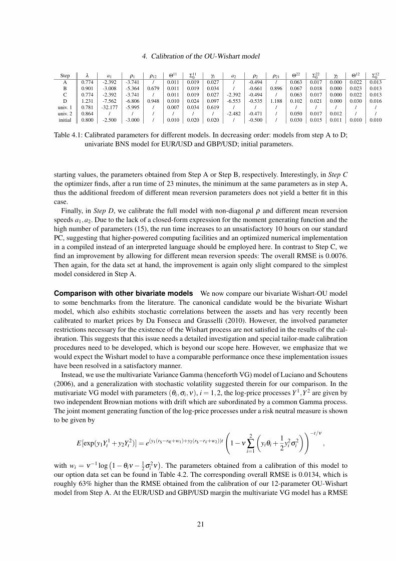
In Step A, we impose a := a1 = a2 and ρ12 = 0 = ρ21, i.e., we make the assumption that the meanreversion parameters of both assets are equal, and that ρ is diagonal. This is the most tractable case,since there is a closed form expression for the moment generating function of (Y 1,Y 2) and the numberof model parameters is reduced to 12. The starting and calibrated parameters can be found in Table 4.1.The overall RMSE is 0.0082, and the run time was 48 minutes, i.e., calibration of the model is feasibleeven on a standard PC. If one considers only the marginal models for EUR/USD and GBP/USD onehas a RMSE of 0.0106 and 0.0048 respectively. For visualisation, we provide Figure 1 and 2, wheremarket and model prices are compared in terms of Black-Scholes implied volatility for a few selectedmaturities. These results illustrate that even this simple model is able to fit the observed smiles ratherwell. For comparison, we calibrated two independent univariate Γ-OU BNS models to the marginsseparately (see Table 4.1) and obtained a lower RMSE of 0.0071 and 0.0020 respectively. This stemsfrom the fact that the additional dependence parameters do not enter the pricing formulae for singleasset options in the diagonal case, whereas the intensity of the compound Poisson process is the samefor all assets in our multivariate framework, unlike when using two univariate models. This means thatwe are not overfitting the marginal distributions with an excessive amount of additional parameters,
18
4. Calibration of the OU-Wishart model
0.9 0.95 1 1.05 1.10
0.2
0.4
0.6
0.8EUR/USD, 2 days
Moneyness K/S0
Impl
ied
Vol
atili
ty
0.8 0.9 10.1
0.2
0.3
0.4
0.5EUR/USD, 23 days
Moneyness K/S0
Impl
ied
Vol
atili
ty
0.9 1 1.10.1
0.15
0.2EUR/USD, 89 days
Moneyness K/S0
Impl
ied
Vol
atili
ty
0.8 0.9 1 1.1 1.20.1
0.15
0.2EUR/USD, 218 days
Moneyness K/S0
Impl
ied
Vol
atili
ty
0.95 1 1.050.12
0.14
0.16
0.18GBP/USD, 15 days
Moneyness K/S0
Impl
ied
Vol
atili
ty
0.9 0.95 1 1.05 1.10.1
0.12
0.14
0.16GBP/USD, 35 days
Moneyness K/S0
Impl
ied
Vol
atili
ty
0.9 0.95 1 1.05 1.10.1
0.12
0.14
0.16
0.18GBP/USD, 166 days
Moneyness K/S0
Impl
ied
Vol
atili
ty
0.9 1 1.1 1.2 1.30.1
0.12
0.14
0.16
0.18GBP/USD, 231 days
Moneyness K/S0
Impl
ied
Vol
atili
ty
Figure 1: Comparison of the Black-Scholes implied volatility of market prices (dot) and model prices(solid line). The plots only show the results for the 12-parameter OU Wishart model (StepA), since they do not change visually for the more complex models from Step B to D.
19
4. Calibration of the OU-Wishart model
0.94 0.96 0.98 1 1.020.1
0.12
0.14
0.16EUR/GBP, 15 days
Moneyness K/S0
Impl
ied
Vol
atili
ty
0.9 1 1.10.1
0.15
0.2
0.25EUR/GBP, 35 days
Moneyness K/S0
Impl
ied
Vol
atili
ty
0.8 0.9 1 1.1 1.20.11
0.12
0.13
0.14
0.15
0.16EUR/GBP, 105 days
Moneyness K/S0
Impl
ied
Vol
atili
ty
0.8 0.9 1 1.1 1.20.11
0.12
0.13
0.14
0.15EUR/GBP, 166 days
Moneyness K/S0
Impl
ied
Vol
atili
ty
Figure 2: Comparison of the Black-Scholes implied volatility of market prices (dot) and model prices(solid line). The plots only show the results for the 12-parameter OU Wishart model (StepA), since they do not change visually for the more complex models from Step B to D.
but much rather using a simplified version of a standard model. Nevertheless, the calibration stillperforms quite well even when using this simplification.
As a further cross-check, Figure 3 depicts sample paths of the EUR/USD and The GBP/USD spotrate and its volatility, simulated with our calibrated parameters, which show reasonable path proper-ties.
In Step B, we allow for a non-diagonal leverage operator ρ . Although this introduces two additionalparameters, ρ12 and ρ21, a closed form expression for the moment generating function is still available.As initial values, we take the parameters obtained in Step A and set ρ12 and ρ21 to zero. After 80minutes, the optimizer finds a minimum with a RMSE of 0.0079. At the margins, we have RMSEsof 0.0104 and 0.0037, respectively. Hence, calibration is still feasible without resorting to higher-powered computers, but the gains in fitting accuracy appear to be only moderate for the option pricesurface at hand.
Next, we drop the assumption of an equal mean reversion parameter and allow for a1 6= a2. Sincethe moment generating function of (Y 1,Y 2) is then not known in closed form anymore, good startingvalues are particularly important in order to reduce computational time to an acceptable value. Wedistinguish the two cases where ρ is diagonal (Step C) and ρ is non-diagonal (Step D), and take as
Table 4.1: Calibrated parameters for different models. In decreasing order: models from step A to D;univariate BNS model for EUR/USD and GBP/USD; initial parameters.
starting values, the parameters obtained from Step A or Step B, respectively. Interestingly, in Step Cthe optimizer finds, after a run time of 23 minutes, the minimum at the same parameters as in step A,thus the additional freedom of different mean reversion parameters does not yield a better fit in thiscase.
Finally, in Step D, we calibrate the full model with non-diagonal ρ and different mean reversionspeeds a1,a2. Due to the lack of a closed-form expression for the moment generating function and thehigh number of parameters (15), the run time increases to an unsatisfactory 10 hours on our standardPC, suggesting that higher-powered computing facilities and an optimized numerical implementationin a compiled instead of an interpreted language should be employed here. In contrast to Step C, wefind an improvement by allowing for different mean reversion speeds: The overall RMSE is 0.0076.Then again, for the data set at hand, the improvement is again only slight compared to the simplestmodel considered in Step A.
Comparison with other bivariate models We now compare our bivariate Wishart-OU modelto some benchmarks from the literature. The canonical candidate would be the bivariate Wishartmodel, which also exhibits stochastic correlations between the assets and has very recently beencalibrated to market prices by Da Fonseca and Grasselli (2010). However, the involved parameterrestrictions necessary for the existence of the Wishart process are not satisfied in the results of the cal-ibration. This suggests that this issue needs a detailed investigation and special tailor-made calibrationprocedures need to be developed, which is beyond our scope here. However, we emphasize that wewould expect the Wishart model to have a comparable performance once these implementation issueshave been resolved in a satisfactory manner.
Instead, we use the multivariate Variance Gamma (henceforth VG) model of Luciano and Schoutens(2006), and a generalization with stochastic volatility suggested therein for our comparison. In themutivariate VG model with parameters (θi,σi,ν), i = 1,2, the log-price processes Y 1,Y 2 are given bytwo independent Brownian motions with drift which are subordinated by a common Gamma process.The joint moment generating function of the log-price processes under a risk neutral measure is shownto be given by
E[exp(y1Y 1t + y2Y 2
t )] = e(y1(r$−re+w1)+y2(r$−r£+w2))t
(1−ν
2
∑i=1
(yiθi +
12
y2i σ
2i
))−t/ν
,
with wi = ν−1 log(1−θiν− 1
2 σ2i ν). The parameters obtained from a calibration of this model to
our option data set can be found in Table 4.2. The corresponding overall RMSE is 0.0134, which isroughly 63% higher than the RMSE obtained from the calibration of our 12-parameter OU-Wishartmodel from Step A. At the EUR/USD and GBP/USD margin the multivariate VG model has a RMSE
21
4. Calibration of the OU-Wishart model
0 100 200 3000
0.005
0.01
0.015
0.02
0.025Σ11, simulated path
Time in trading days
Vol
atili
ty o
f EU
R/U
SD
Spo
t
0 100 200 3000
0.005
0.01
0.015
0.02
0.025
0.03Σ22, simulated path
Time in trading days
Vol
atili
ty o
f GB
P/U
SD
Spo
t
0 100 200 300
1.25
1.3
1.35
1.4
1.45EUR/USD Spot, simulated path
Time in trading days
Val
ue o
f 1 E
UR
in U
SD
0 100 200 300
1.5
1.55
1.6
1.65
1.7GBP/USD Spot, simulated path
Time in trading days
Val
ue o
f 1 G
BP
in U
SD
Figure 3: Simulated sample path of the EUR/USD and the GBP/USD spot rate and its volatility in the12-parameter OU-Wishart model (Step A).
of 0.0161 and 0.0107. Consequently, the performance of this model is much worse than for the OU-Wishart model, which is not surprising since it only involves 5 parameters.
To alleviate this issue, our second benchmark allows for stochastic activity driven by an OU typeprocess. More specifically, the log-price processes of the EUR/USD and GBP/USD spot rate are givenby Y 1
t = X1Zt
and Y 2t = X2
Zt, where X1 and X2 are two independent Variance Gamma processes with
parameters (θi,σi,νi), i = 1,2, and Zt =∫ t
0 zsds is an integrated Ornstein-Uhlenbeck process. TheOrnstein-Uhlenbeck process (zs)s∈R+ is given by dzs = 2αzsds+dN−2αt ,z0 = 1, α < 0, where N is acompound Poisson process with intensity ϑ and EXP(ξ ) distributed jumps. It can be shown that themoment generating function of Zt , see e.g. (Schoutens; 2003, 7.2.2), is given by
For the moment generating function of Yt = (Y 1t ,Y
2t ), conditioning on the stochastic activity process
Z yields
ΦYt (y1,y2) = ΦZt
(logΦX1
1(y1)+ logΦX2
1(y2)
)
22
4. Calibration of the OU-Wishart model
0.8 0.85 0.9 0.95 1 1.050.1
0.15
0.2
0.25
0.3
0.35EUR/USD, 23 days
Moneyness K/S0
Impl
ied
Vol
atili
ty
0.94 0.96 0.98 1 1.02 1.04 1.060.1
0.12
0.14
0.16GBP/USD, 35 days
Moneyness K/S0
Impl
ied
Vol
atili
ty
0.85 0.9 0.95 1 1.05 1.10.1
0.15
0.2
0.25EUR/GBP, 35 days
Moneyness K/S0
Impl
ied
Vol
atili
ty
0.8 0.9 1 1.1 1.20.11
0.12
0.13
0.14
0.15
0.16EUR/GBP, 105 days
Moneyness K/S0
Impl
ied
Vol
atili
ty
Figure 4: Comparison of the Black-Scholes implied volatility of market prices (dot) and model prices(solid line). The headers state the underlying and the days to maturity. The plots are forthe benchmark model where the log-price processes are modelled by two independent VGprocesses with a common time change which is given by an integrated Γ-OU process. Theplots for the multivariate VG model from Luciano and Schoutens (2006) look visually thesame.
with ΦX i1(yi) =
(1− yiθiνi− 1
2 σ2i y2
i νi)−1/νi , i = 1,2. Thus, the joint moment generating function of
the log-price processes Y 1t ,Y
2t under a risk neutral measure is given by
ΦYt (1,0)−y1ΦYt (0,1)
−y2ΦYt (y1,y2).
A calibration of this model to our dataset leads to the parameters provided in Table 4.2; a plot depict-ing some of the respective implied volatilities can be found in Figure 4. The corresponding RMSEis 0.0129. Somewhat surprisingly, this is only around 4% lower than for the model of Luciano andSchoutens (2006), despite increasing the number of parameters from 5 to 9. At the margins, we have0.0143 and 0.0095, which corresponds to improvements of around 11%. Hence, there is quite someimprovement in fitting the margins, but the fit for the multivariate options is actually slightly worse.Moreover, further numerical experiments suggest that, to recapture our spread option prices, one needsquite extreme parameter values, which do not match well with the univariate option prices. This sug-gests that stochastic correlations indeed seem necessary to recapture the features of our empiricaldataset. However, let us emphasize again that this only applies to one specific dataset in the foreignexchange market. A more detailed empirical study is a challenging topic for future research.
Table 4.2: The first row shows the calibrated parameters for the multivariate VG model of Luciano andSchoutens (2006). The second row contains the calibrated parameters for two independentVG processes with a common integrated Γ-OU time change.
5. Covariance swaps
In this final section, we show that it is possible to price swaps on the covariance between differentassets in closed form. This serves two purposes. On the one hand, options written on the realised cov-ariance represent a family of payoffs that only make sense in models where covariances are modelledas stochastic processes rather than constants. On the other hand, the ensuing calculations exemplifyonce more the analytical tractability of the present framework.
We consider again our multivariate stochastic volatility model of OU type under an EMM Q. In ad-dition, we suppose that the matrix subordinator L is square integrable, i.e.
∫||X ||>1 ||X ||2κL(dX)< ∞.
The pricing of options written on the realised variance resp. the quadratic variation as its continuous-time limit have been studied extensively in the literature, cf., e.g., Carr and Lee (2008) and the ref-erences therein. Since we have a nontrivial correlation structure in our model, one can also considercovariance swaps on two assets i, j ∈ 1, . . . ,d, i.e., contracts with payoff [Y i,Y j]T −K with covari-ance swap rate K = E([Y i,Y j]T ) (see, e.g., Carr and Madan (1999a), Da Fonseca, Grasselli and Ielpo(2008), or Swischuk (2005) for more background on these products). Now, we show how to computethe covariance swap rate. We have
[Y i,Y j]T = [Y i,Y j]cT + ∑s≤T
∆Y is ∆Y j
s = (Σ+T )
i j +ρi(X)ρ j(X)∗µ
LT (dX).
Since κL(dX)dt is the compensator of µL, this yields
E([Y i,Y j]T ) = (E(Σ+T ))
i j +T∫S+d
ρi(X)ρ j(X)κL(dX), (5.1)
where Σ+T was defined in Equation (2.4). Note that by Pigorsch and Stelzer (2009, Proposition 2.4)
and since |ρ i(X)ρ j(X)| ≤ ||ρ||2||X ||2, our integrability assumption on L implies that the expectationis finite. The first summand can be calculated as follows. By setting y = 0 in Theorem 2.5 we obtainthe characteristic function of Σt . Differentiation yields
so we only need to know E(L1). The second summand in (5.1) can analogously be computed bydifferentiating the characteristic function of the matrix subordinator L.
In our OU-Wishart model, where L is a compound Poisson matrix subordinator plus drift withWd(n,Θ)-distributed jumps, we have by Gupta and Nagar (2000, Theorem 3.3.15) that
E(L1) = γL +λnΘ.
24
5. Covariance swaps
If ρ is diagonal, the second term in (5.1) simplifies to
T ρiρ j
∫S+d
XiiX j j ν(dX) = T ρiρ jλn(2Θ
2i j +nΘiiΘ j j
),
again by Gupta and Nagar (2000, Theorem 3.3.15). Thus we have a closed form expression for thecovariance swap rate:
For example, in the 2-dimensional OU-Wishart model from Section 4.1 we have for i = 1 and j = 2
K =1
a1 +a2
[(e(a1+a2)T −1
)(Σ
120 +
λnΘ12
a1 +a2
)−T λnΘ12
]+T ρ1ρ2λn
(2Θ
212 +nΘ11Θ22
).
As an illustration we provide, in Figure 5, a plot of the normalized covariance swap rate measured in
volaility points, i.e., T 7→√
1T E([Y 1,Y 2]T ), for our calibrated 12-parameter OU-Wishart model from
Section 4.2 (Step A).
0 50 100 150 200 250 3000.12
0.125
0.13
0.135
0.14Covariance swap rate normalized by maturity in volatility points
Time to maturity in trading days
Figure 5: Normalized covariance swap rate for the calibrated 12-parameter OU-Wishart model.
Finally, we remark that similarly as in Carr and Lee (2008), pricing of options on the covariancecan be dealt with using the Fourier methods from Section 3, since the joint characteristic function of(Σ+,ρ i(X)ρ j(X)∗µL(dX)) can be calculated similarly as in the proof of Theorem 2.5.
Acknowledgements
The first author gratefully acknowledges support from the FWF (Austrian Science Fund) under grantP19456 and by the National Centre of Competence in Research “Financial Valuation and Risk Man-agement” (NCCR FINRISK), Project D1 (Mathematical Methods in Financial Risk Management).
25
A. Appendix
The NCCR FINRISK is a research instrument of the Swiss National Science Foundation. The secondand third author greatly appreciate the support of the Technische Universitat Munchen - Institute ofAdvanced Study, the second author additionally the one by the International Graduate School of Sci-ence and Engineering, funded by the German Excellence Initiative.
The authors thank Christa Cucchiero for fruitful discussions. They are also grateful to two anonym-ous referees and an anonymous associate editor for their numerous helpful comments, that signific-antly improved the present article.
A. Appendix
The following result on multidimensional analytic functions is needed in the proof of Lemma 2.7.
Lemma A.1. Let Dε = z ∈ Cn : ||Re(z)|| < ε for some ε > 0. Suppose f : Dε → C is an analyticfunction of the form f = eF , where F : Dε → C is continuous. Then F is analytic in Dε .
Proof. Let z = (z1,z2, . . . ,zn) ∈ Dε and define z−1 = (z2, . . . ,zn). Then fz−1 : w 7→ f (w,z−1) definesan analytic function without zeros on the open convex set Dε,z−1 := w ∈ C : (w,z−1) ∈ Dε. Bye.g. Fischer and Lieb (1994, Satz V.1.4), there exists an analytic function g1
z−1: Dε,z−1 → C such that
exp(g1z−1
) = fz−1 . Hence F(w,z−1)− g1z−1
(w) ∈ 2πiZ on Dε,z−1 . Since both F and g are continuous,their difference is constant and it follows that w 7→ F(w,z−1) is analytic on Dε,z−1 . Analogously, oneshows analyticity of F in all other components. The assertion then follows from Hartog’s Theorem(cf. e.g. Hormander (1967, Theorem 2.2.8)).
ReferencesBarndorff-Nielsen, O. E. and Perez-Abreu, V. (2008). Matrix subordinators and related upsilon transformations,
Theory of Probability and Its Applications 52: 1–23.
Barndorff-Nielsen, O. E. and Shepard, N. (2001). Non-Gaussian Ornstein-Uhlenbeck-based models and someof their uses in financial economics, Journal of the Royal Statistical Society B 63: 167–241.
Barndorff-Nielsen, O. E. and Stelzer, R. (2007). Positive-definite matrix processes of finite variation, Probab-ility and Mathematical Statistics 27: 3–43.
Barndorff-Nielsen, O. E. and Stelzer, R. (2011). The multivariate supOU stochastic volatility model, Mathem-atical Finance . To appear.
Benth, F. E. and Vos, L. (2009). A multivariate non-Gaussian stochastic volatility model with leverage forenergy markets, Preprint. Available from http://www.math.uio.no/eprint/pure_math/2009/.
Carr, P. and Lee, R. (2008). Robust replication of volatility derivatives, Preprint. Available from http://www.
math.uchicago.edu/~rl.
Carr, P. and Madan, D. (1999a). Introducing the covariance swap, RISK pp. 47–52.
Carr, P. and Madan, D. B. (1999b). Option valuation using the Fast Fourier Transform, Journal of Computa-tional Finance 2: 61–73.
Cont, R. and Tankov, P. (2004). Financial Modelling with Jump Processes, Chapman & Hall/CRC, Boca Raton.
Cuchiero, C., Filipovic, D., Mayerhofer, E. and Teichmann, J. (2010). Affine processes on positive semidefinitematrices, Annals of Applied Probability 21: 397–463.
Da Fonseca, J. and Grasselli, M. (2010). Riding on the smiles, Preprint. Available at http://papers.ssrn.com/sol3/papers.cfm?abstract_id=1663448.
Da Fonseca, J., Grasselli, M. and Ielpo, F. (2008). Hedging (co)variance risk with variance swaps, InternationalJournal of Theoretical and Applied Finance . To appear.
Da Fonseca, J., Grasselli, M. and Tebaldi, C. (2007). Option pricing when correlations are stochastic: ananalytical framework, Review of Derivatives Research 10: 151–180.
Dimitroff, G., Lorenz, S. and Szimayer, A. (2010). A parsimonious multi-asset Heston model: Calibration andderivative pricing, International Journal of Theoretical and Applied Finance . To appear.
Duffie, D., Filipovic, D. and Schachermayer, W. (2003). Affine processes and applications in finance, Annalsof Applied Probability 13: 984–1053.
Duffie, D., Pan, J. and Singleton, K. (2000). Transform analysis and asset pricing for affine jump-diffusions,Econometrica 68: 1343–1376.
Eberlein, E., Glau, K. and Papapantoleon, A. (2009). Analysis of Fourier transform valuation formulas andapplications, Applied Mathematical Finance 17: 211–240.
Eberlein, E. and Raible, S. (1999). Term structure models driven by general Levy processes, MathematicalFinance 9: 31–53.
Fischer, W. and Lieb, I. (1994). Funktionentheorie, Vieweg, Braunschweig.
Gourieroux, C. (2007). Continuous time Wishart process for stochastic risk, Econometric Reviews 25: 177–217.
Gourieroux, C. and Sufana, R. (2010). Derivative pricing with wishart multivariate stochastic volatility, Journalof Business & Economic Statistics 28: 438–451.
Gradshteyn and Ryzhik (2007). Table of Integrals, Series, and Products, Academic Press, Amsterdam.
Gupta, A. K. and Nagar, D. K. (2000). Matrix Variate Distributions, Chapman & Hall/CRC, Boca Raton.
Heston, S. L. (1993). A closed-form solution for options with stochastic volatility with applications to bondand currency options, Review of Financial Studies 6: 327–343.
Horn, R. A. and Johnson, C. R. (1990). Matrix Analysis, Cambridge University Press, Cambridge.
Hubalek, F. and Nicolato, E. (2005). On multivariate extensions of Levy driven Ornstein-Uhlenbeck typestochastic volatility models and multi-asset options, Preprint.
Hull, J. C. (2003). Options, Futures and other Derivatives, Prentice-Hall, Upper Saddle River, NJ.
Hurd, T. R. and Zhou, Z. (2010). A Fourier transform method for spread option pricing, SIAM Journal onFinancial Mathematics 1: 142–157.
Hormander, L. (1967). An Introduction to Complex Analysis in Several Variables, D. Van Nostrand, Princeton.
Jacod, J. and Shiryaev, A. N. (2003). Limit Theorems for Stochastic Processes, 2nd edn, Springer, Berlin.
Jacod, J. and Todorov, V. (2010). Do price and volatility jump together?, Annals of Applied Probability20: 1425–1469.
Kallsen, J. (2006). A didactic note on affine stochastic volatility models, in Y. Kabanov, R. Liptser and J. Stoy-anov (eds), From Stochastic Calculus to Mathematical Finance, Springer, Berlin, pp. 343–368.
Konigsberger, K. (2004). Analysis 2, 5th edn, Springer, Berlin.
Luciano, E. and Schoutens, W. (2006). A multivariate jump-driven financial asset model, Quantitative Finance6: 385–402.
Ma, J. (2009). A Stochastic Correlation Model with Mean Reversion for Pricing Multi-Asset Options, Asia-Pacific Financial Markets 16: 97–109.
Margrabe, W. (1978). The value of an option to exchange one asset for another, Journal of Finance 33: 177–186.
Nicolato, E. and Venardos, E. (2003). Option pricing in stochastic volatility models of the Ornstein-Uhlenbecktype, Mathematical Finance 13: 445–466.
Pigorsch, C. and Stelzer, R. (2009). A multivariate Ornstein-Uhlenbeck type stochastic volatility model, Pre-print. Available from http://www.uni-ulm.de/mawi/finmath.html.
Raible, S. (2000). Levy Processes in Finance: Theory, Numerics, and Empirical Facts, PhD thesis, UniversitatFreiburg i. Br.
Rajput, B. and Rosinski, J. (1989). Spectral Representations of Infinitely Divisible Processes, ProbabilityTheory and Related Fields 82: 451–487.
Sato, K. (1999). Levy Processes and Infinitely Divisible Distributions, Cambridge University Press, Cambridge.
Schoutens, W. (2003). Levy Processes in Finance., Wiley, New York.
Swischuk, A. (2005). Modeling of variance and volatility swaps for financial markets with stochastic volatility,WILMOTT Magazine pp. 64–72.
Taylor, S. J. and Wang, Y. (2010). Option prices and risk neutral densities for currency cross rates, Journal ofFutures Markets 30: 324–360.