European Journal of Operational Research 223 (2012) 762–774

Contents lists available at SciVerse ScienceDirect

European Journal of Operational Research

journal homepage: www.elsevier .com/locate /e jor

Innovative Applications of O.R.

Option pricing under a normal mixture distribution derived from the Markovtree model

Harish S. Bhat ⇑, Nitesh KumarSchool of Natural Sciences, University of California, Merced, 5200 N. Lake Rd., Merced, CA 95343, USA

a r t i c l e i n f o

Article history:Received 13 July 2011Accepted 4 July 2012Available online 17 July 2012

Keywords:FinanceOptions pricingAsymptotic analysisMixture modelsEmpirical testing

0377-2217/$ - see front matter � 2012 Elsevier B.V. Ahttp://dx.doi.org/10.1016/j.ejor.2012.07.003

⇑ Corresponding author. Tel.: +1 209 617 5806.E-mail address: hbhat@ucmerced.edu (H.S. Bhat).

a b s t r a c t

We examine a Markov tree (MT) model for option pricing in which the dynamics of the underlying assetare modeled by a non-IID process. We show that the discrete probability mass function of log returnsgenerated by the tree is closely approximated by a continuous mixture of two normal distributions. Usingthis normal mixture distribution and risk-neutral pricing, we derive a closed-form expression for Euro-pean call option prices. We also suggest a regression tree-based method for estimating three volatilityparameters r, r+, and r� required to apply the MT model. We apply the MT model to price call optionson 89 non-dividend paying stocks from the S&P 500 index. For each stock symbol on a given day, we usethe same parameters to price options across all strikes and expires. Comparing against the Black–Scholesmodel, we find that the MT model’s prices are closer to market prices.

� 2012 Elsevier B.V. All rights reserved.

1. Introduction

The Black–Scholes model for European call options assumesthat the underlying asset follows a geometric Brownian motion:if St is the price of the underlying at time t, then dSt = lStdt +rStdWt, where l and r are constants and Wt is a Brownian motion.It follows that the Black–Scholes model assumes normality of dailylog returns and independence of increments. The purpose of thispaper is the detailed examination, both theoretical and empirical,of a model in which both assumptions are removed. This modelwas introduced as the Markov tree (MT) model in our earlier work(Bhat and Kumar, 2010). The name of the model indicates that thetree is a generalization of the standard binomial tree, where theup/down factors at step n + 1 depend on the direction of the steptaken at step n. This is illustrated in Fig. 1. Though the descriptionof the model is simple, and though it contains only two additionalstatic parameters (r+ and r�) that must be estimated from data,the MT model leads to a number of non-trivial properties with sig-nificant consequences for option pricing.

By construction, the MT model accounts for the serial depen-dence of log returns. As we show, the distribution generated bythe MT model is very closely approximated by a mixture of nor-mals. Though this topic is not pursued further here, the MT modelis a tree model that could be used to price path-dependent options.Hence the MT model can be seen as combining the strengths ofnormal mixture models, non-IID models, and tree methods allwithin the framework of risk-neutral pricing. In this paper, we

ll rights reserved.

derive an accurate, computationally efficient, closed-form approx-imation to the MT model option price. We proceed to subject ourmodel to out-of-sample comparisons against market prices andBlack–Scholes model prices.

The MT model incorporates several features that have beenstudied separately in the literature. The first such feature is theuse of a mixture of normals. It is widely accepted that the observeddistribution of daily log returns for stocks has heavier tails than thenormal distribution, skewness, and positive excess kurtosis (Cont,2001; Campbell et al., 1997; Barone-Adesi, 1985; Longin, 2005;Behr and Pötter, 2009). Many distributions have been proposedto match these properties. These distributions can be classified intoparametric and non-parametric models—for an extensive list, see(Jackwerth, 1999). Parametric models include generalized distribu-tions (Eberlein and Keller, 1995) and mixture distributions (Kon,1984). Empirical tests (Behr and Pötter, 2009) conclude that nor-mal mixture models fit observed log returns better than other gen-eralized parametric models. In recent work, mixture distributionshave been used in both option pricing and portfolio optimization(Tan and Chu, 2012; Cai and Kou, 2011, Ramponi, 2011, Buckleyet al., 2008; Brigo and Mercurio, 2002; Ritchey, 1990) with success.

The second feature of the MT model is the non-IID process usedto model the underlying asset dynamics. The study of (Niederhof-fer and Osborne, 1966) was one of the first to examine serialdependence of log returns, providing strong evidence of depen-dence in tick differences. Daily returns have been studied by manyauthors, e.g., (Fielitz and Bhargava, 1973; Fielitz, 1975; Ding et al.,1993; Taylor, 2007), providing considerable evidence that daily re-turns are not independent. For returns sampled at longer intervals,i.e., monthly or yearly, the evidence is inconclusive (Sewell, 2011).

d

u

v

v

v

v

v

v

v

w

w

w

w

w

w

w

x

x

x

x

x

x

x

y

y

y

y

y

y

y

Fig. 1. Tree of depth n = 6 showing recombination of paths of the underlying assetin the MT model. The asset begins with price S0 and is multiplied by the weightsalong the path. For example, a possible path of length 3 shown here is S0u w x. Boththe probabilities and the outcomes of Sn+1/Sn depend on whether Sn/Sn�1 was anupward or downward movement. In this way, the tree accounts for first-orderMarkov dependence of log returns. At depth n, there are n2 � n + 2 possible states,as shown in Section 3.2.

H.S. Bhat, N. Kumar / European Journal of Operational Research 223 (2012) 762–774 763

Note that the short-term dependence of log returns need not inval-idate the weak form of the efficient market hypothesis (Fama,1970).

Several option pricing models have been proposed that allowfor serial dependence of the underlying asset’s returns. A direct ap-proach is to explicitly account for dependence on the past in theunderlying asset model. This strategy has been pursued with Mar-kov and semi-Markov processes (Janssen et al., 1997; D’Amicoet al., 2009), jump-diffusion processes with non-IID jumps (Camaraand and Li, 2008), and stochastic delay differential equations(SDDEs) (Appleby et al., 2012a; Appleby et al., 2012b; Changet al., 2011; Chang et al., 2010;Swords and Appleby, 2010; Wuet al., 2008; Chang and Youree, 2007; Kazmerchuk et al., 2007;Arriojas et al., 2007). In the case of SDDE models, obtaining aclosed-form approximation for the option price is much more dif-ficult than for the MT model. Furthermore, when SDDE models areproposed in the literature, the performance of the models has notbeen tested using market data.

Another approach that yields a non-IID model is to introducethe concept of a regime; in a regime-switching model, a stochasticprocess (typically, a Markov chain) drives the regime from onestate to another, and model parameters such as volatility and therisk-free rate are functions of the regime state (Mamon and Rodr-igo, 2005; Aingworth et al., 2006; Basu and Ghosh, 2009). Finally,we note that in the framework of stochastic and/or GARCH volatil-ity (Heston, 1993; Heston and Nandi, 2000) models, non-IID re-turns are a side effect of a volatility process that allows formemory.

The general outline of this paper is as follows. In Section 2, wereview the definition of the MT model and the properties estab-lished in (Bhat and Kumar, 2010). Then, in Section 3, we prove that

the tree is recombinant and give an exact formula for the optionprice. The exact formula relies on a discrete p.m.f. (probabilitymass function) that becomes prohibitively difficult to compute asthe size of the time step vanishes. Therefore, in Section 4, weapproximate the p.m.f. by a continuous p.d.f. (probability densityfunction), which turns out to be a mixture of normal distributions.In Section 5, we use the approximate continuous p.d.f. to derive aclosed-form option price. In Section 6, we conduct out-of-sampleempirical tests that show that the MT model’s prices are very closeto market prices. In the same section, we give our conclusions anddirections for further research.

2. Review of the Markov tree model

To keep this paper self-contained, we review the main points of(Bhat and Kumar, 2010).

2.1. Underlying asset dynamics

The Markov tree (MT) models the up and down movements inthe underlying asset as a first-order Markov chain. The total timeto expiration Y (in years) is divided into N equispaced steps withDt = Y/N years. Let Sn be the asset price at time step n. For n = 0,let the magnitudes of the up/down movements be u and d, andlet the probability of an up movement be q. Then P(S1 = S0u) = q,and P(S1 = S0d) = 1 � q.

For n P 1, the model departs from the standard binomial optionpricing model. We define two new events Sþn ¼ fSn P Sn�1g andS�n ¼ fSn < Sn�1g; these events correspond to an upward (Sþn ) ordownward (S�n ) movement in price from time step n � 1 to timestep n.

For n P 1, we define the evolution of the tree using two newprobabilities q+ and q�:

P Snþ1 ¼ SnvjSþn� �

¼ qþ; P Snþ1 ¼ SnwjSþn� �

¼ 1� qþ; andP Snþ1 ¼ SnxjS�n� �

¼ q�; P Snþ1 ¼ SnyjS�n� �

¼ 1� q�:

We have introduced four symbols v,w,x and y that are factors bywhich the stock price at any step is allowed to change. The stockprice goes up or down by a factor of v or w (respectively, x or y) ifthe stock price increased (respectively, decreased) in the previousstep of the tree. See Fig. 1 for a pictorial representation of the tree,showing its recombinant behavior for n P 4. In Section 3, we showthat the number of nodes at depth n of the tree is n2 � n + 2, far lessthan the worst-case behavior of 2n for a non-recombinant tree.

2.2. Martingale property

Let r be the risk-free rate of interest. We define

q¼ expðrDtÞ�du�d

; qþ ¼ expðrDtÞ�wv �w

; q� ¼ expðrDtÞ�yx�y

: ð1Þ

Then one checks that E[S1jS0] = u S0q + d S0(1 � q) = erDt S0, and forn P 1,

E½Snþ1jSn; . . . ; S0� ¼ E Snþ1jSn; . . . ; S0; Sþn

� �P Sþn� �

þ E Snþ1jSn; . . . ; S0; S�n

� �P S�n� �

¼ vSnqþ þwSnð1� qþÞ½ �P Sþn� �

þ xSnq� þ ySnð1� q�Þ½ �P S�n� �

¼ erDtSnP Sþn� �

þ erDtSnP S�n� �

¼ erDtSn:

This implies that the discounted process Sn ¼ e�rnDtSn is a martingaleunder the risk-neutral probabilities (1). By standard arguments, thisimplies that the MT model does not admit arbitrage (see (Shreve,2004, Chapter 2.4)).

764 H.S. Bhat, N. Kumar / European Journal of Operational Research 223 (2012) 762–774

2.3. Risk-neutral pricing

Let us now use the Markov tree to price a European call optionwith strike K and spot price S0. We defer all details on statisticalestimation of the parameters r,u,d,v,w,x, and y to Section 6—atthe moment, we take these parameters as given. Then, using theMarkov tree and (1), we generate a risk-neutral p.m.f. for the ran-dom variable SN, the share price of the underlying asset at the timeof expiry. Let JN denote the set of possible outcomes of SN. Finally,for a random variable X(x), let X+(x) denote the random variable

XþðxÞ ¼XðxÞ XðxÞ > 00 XðxÞ 6 0:

�Then the MT model’s call options price is the discounted expectedvalue of the option’s payoff:

C ¼ e�rY E½ðSN � KÞþ� ð2Þ

Using the exact p.m.f. generated by the Markov tree, we have

C ¼ e�rYXr2JNr>K

ðr� KÞPðSN ¼ rÞ: ð3Þ

The MT model has been subjected to out-of-sample tests againstmarket prices of European options. We used the MT model to priceoptions on six stocks from the French CAC-40 index. Across 44 daysof testing, the MT model’s prices more closely matched marketprices than the Black–Scholes model’s prices (Bhat and Kumar,2010).

3. Markov tree generation and computational tractability

Here we establish that the maximum number of possible statesin a Markov tree of depth n is n2 � n + 2. We also give a method forcomputing the p.m.f. of Sn, the underlying asset price after n stepsof the tree.

3.1. Persistent random walk

The time evolution of eSn ¼ log Sn under the Markov tree isequivalent to a persistent random walk on the real line, where boththe size and direction of the walker’s step at time step n + 1 de-pends on the direction of the step taken at time step n:eSnþ1ðxÞ ¼ eSnðxÞ þ GðHðeSn � eSn�1Þ;xÞ; ð4Þ

where H is the Heaviside function

HðxÞ ¼1 x > 00 x < 0;

�and G(1,x),G(0,x) are random variables with p.m.f.’s

PðGð1;xÞ ¼ log vÞ ¼ qþ; PðGð1;xÞ ¼ log wÞ ¼ 1� qþ; andPðGð0;xÞ ¼ log xÞ ¼ q�; PðGð0;xÞ ¼ log yÞ ¼ 1� q�

for n P 2. For n = 1, the p.m.f. of G(1,x) and G(0,x) is given by

PðGð1;xÞ ¼ log uÞ ¼ q

PðGð1;xÞ ¼ log dÞ ¼ 1� q:

We assume logu, logd, logv, logw, logx, logy are all non-zero, sothat PðeSn ¼ eSn�1Þ ¼ 0.

3.2. Number of states in a tree of fixed depth

For the moment, we ignore the size of the walker’s steps and fo-cus only on their direction. If the walker moves to the right(respectively, left), we call that heads H (respectively, tails T). The

walk after n steps can be regarded as a random sequence of headsH and tails T.

Let nH (respectively, nT) be 1 if the first element is H (respec-tively, T) and 0 otherwise. Let nHH,nHT,nTH, and nTT denote the num-ber of subsequences of the form HH,HT, TH, and TT. Then

nHH þ nHT þ nTH þ nTT ¼ n� 1: ð5Þ

Let v = (nH, nT, nHH, nHT, nTH, nTT). The final position of the walker iseSn ¼ eS0 þ s � v where s = (logu, logd, logv, logw, logx, logy). Henceenumerating all possible vectors v is equivalent to enumeratingall possible outcomes of eSn.

Suppose that the sequence starts with H. Let t denote the num-ber of transitions:

t ¼ nHT þ nTH: ð6Þ

Now t can be anything from 0 to n � 1. Given t, we know nHT andnTH, since transitions must alternate H to T and T to H. For t = 0,there is only one sequence HHH � � � H.

For t = 1,2, . . . ,n � 1, a walk with t transitions is a sequence oft + 1 blocks, with odd blocks consisting of consecutive H’s and evenblocks consisting of consecutive T’s. We start with the sequenceHTHTHT� � � of length t + 1. To convert this into a walk of length n,we must insert extra H’s into the H blocks and extra T’s into theT blocks, inserting n � t � 1 elements in total. Now nHH is the num-ber of H’s inserted, so it can be anything from 0 to n � t � 1, forn � t possibilities in total. Once we know nHH, we solve for nTT using(5).

For a walk of length n starting with H, the number of possible v’s

is 1þPn�1

t¼1 ðn� tÞ ¼ 1þ nðn�1Þ2 . Twice this number is n2 � n + 2, the

total number of possibilities for v. Note that the regime-switchingmodel of (Aingworth et al., 2006), if used with two volatility states,results in a different tree that also has quadratic complexity.

3.3. Markov tree probability mass function

Now let us assume v is given and count how many walks corre-spond to that same v. Starting with H, there are a = nTH + 1 blocks ofheads and b = nHT blocks of tails.

Given nHH and nTT, to obtain the walk we must decide how manyof the nHH extra heads to insert into each block, with the total beingnHH. The number of such possibilities is the number of weak com-

positions of nHH into a nonnegative integers, nHH þ a� 1a� 1

� �. We

must also decide how many of the nTT extra tails to insert into eachblock, with the total being nTT. The number of such possibilities isthe number of weak compositions of nTT in b nonnegative integers,

nTT þ b� 1b� 1

� �.

Hence the number of walks that start with H and correspond tov is

#ðvÞ¼nHHþa�1

a�1

� �nTTþb�1

b�1

� �¼

nHHþnTH

nTH

� �nTTþnHT�1

nHT�1:

� �ð7Þ

If instead the walk starts with T, the only difference is that a = nTH

and b = nHT + 1 and we obtain

#ðvÞ¼nHHþa�1

a�1

� �nTTþb�1

b�1

� �¼

nHHþnTH�1nTH�1

� �nTTþnHT

nHT

� �ð8Þ

as the number of walks.Once we know how many ways there are of reaching eSn from eS0,

we can compute

PðeSn ¼ eS0 þ s � vÞ ¼ #ðvÞqv ; ð9Þ

H.S. Bhat, N. Kumar / European Journal of Operational Research 223 (2012) 762–774 765

where q = (q, 1 � q, q+, 1 � q+, q�, 1 � q�) and qv ¼Q6

j¼1qv j

j . In thisway, the entire p.m.f. of eSn is determined.

Care must be used when applying the above formulas, as theydo not detect whether the walk is allowed or not. If the walk cor-responding to v is allowed, then the above formulas give the num-ber of walks.

This begs the question of enumerating all allowed v’s at a fixeddepth n. This can be done using the following algorithm, whichworks for all walks that start with H (so that nH = 1):

print v = (1,0,n � 1,0,0,0)for t = 1 ? n � 1 do

nHT = dt/2enTH = bt/2cfor nHH = 0 ? n � t � 1 do

nTT = (n � t � 1) � nHH

print v = (1,nHH,nHT,nTH,nTT)end for

end for

To enumerate all walks that start with T (so that nT = 1), we usethe same algorithm as above with two minor changes: (i) switchthe definitions of nHT and nTH; (ii) change the t = 0 output of v tobe v = (0,1,0,0,0,n � 1). Using both algorithms, we produce a listof all allowed v’s at a fixed depth n.

4. Continuous approximation of the Markov tree

We can see from (2) that the key ingredient in computing theMarkov tree options price is taking the expected value of the payofffunction with respect to the p.m.f. (9) generated by the tree.Though we have developed an efficient algorithm to generate allstates of the tree, the quantity #(v) defined by (7) and (8) is diffi-cult to compute in finite-precision arithmetic due to the large bino-mial coefficients involved. In this section, we develop a closed-form continuous p.d.f. that closely approximates the discrete Mar-kov tree p.m.f.

The p.d.f., which turns out to be a mixture of normals, alsoyields an intuitive understanding of the distribution of asset pricesgenerated by the Markov tree. This understanding will lead us to areasonable method to statistically estimate the parameters u,v,and x from market data.

4.1. Recursion

To develop a continuous approximation, we first rewrite thediscrete-time process (4) as a recursion. We assume all movementsare symmetric about one (i.e., d = 1/u,w = 1/v,y = 1/x) and define

lu ¼ log u ¼ � log d ð10aÞl1 ¼ log v ¼ � log w ð10bÞl2 ¼ log x ¼ � log y ð10cÞ

We assume lu, l1, and l2 are all positive.Let Rðn;~sÞ be the probability of reaching a value ~s on the real line

in n steps by moving to the right (in the positive direction on R) inthe nth step. Similarly, let Lðn;~sÞ be the probability of reaching thevalue ~s in n steps by moving to the left (in the negative direction onR) in the nth step.

In the Markov tree, since log v and log x are the only positivesteps allowed, Rðn;~sÞ is the probability of reaching ~s in n steps bytaking either a logv step or a logx step in the nth step. If the nthstep was a logv step, then after n � 1 steps, the walker was at~s� l1 and had reached there by taking the (n � 1)th step to the

right. The probability of the walker reaching this position in thisway after n � 1 steps is Rðn� 1;~s� l1Þ. Similarly, if the nth stepwas a logx step, then after n � 1 steps, the walker was at ~s� l2

and had reached there by taking the (n � 1)th step to the left.The probability of the walker reaching this position in this wayafter n � 1 steps is Lðn� 1;~s� l2Þ.

Putting things together, we obtain

Rðn;~sÞ ¼ qþRðn� 1;~s� l1Þ þ q�Lðn� 1;~s� l2Þ: ð11Þ

Next, since logw and logy are the only negative steps in the Markovtree, Lðn;~sÞ is the probability of reaching ~s in n steps by taking alogw step or a log y step in the nth step. If the nth step was a logwstep, then the walker was at ~sþ l1 after n � 1 steps and had reachedthere by taking the (n � 1)th step to the right. The probability of thewalker reaching this position in this way after n � 1 steps isRðn� 1;~sþ l1Þ. Similarly, if the nth step was a logy step, then therandom walker was at ~sþ l2 after n � 1 steps and had reached thereby taking the (n � 1)th step to the left. The probability of the walkerreaching this position in this way after n � 1 steps is Lðn� 1;~sþ l2Þ.

Putting things together, we obtain

Lðn;~sÞ ¼ ð1� qþÞRðn� 1;~sþ l1Þ þ ð1� q�ÞLðn� 1;~sþ l2Þ: ð12Þ

4.2. Exact solution in Fourier space

We introduce the following forward and inverse Fourier trans-form pair, with the variable k as the Fourier conjugate variable to ~s:

f̂ ðkÞ ¼Z

R

f ð~sÞe�ik~sd~s; f ð~sÞ ¼ 12p

ZR

f̂ ðkÞeik~sdk: ð13Þ

Define

M ¼ qþe�ikl1 q�e�ikl2

ð1� qþÞeikl1 ð1� q�Þeikl2

" #: ð14Þ

Then, taking the Fourier transforms of both sides of (11) and (12),we are able to put the system into matrix–vector form and solve:bRðn; kÞbLðn; kÞ" #

¼ MbRðn� 1; kÞbLðn� 1; kÞ

" #¼ Mn�1

bRð1; kÞbLð1; kÞ" #

: ð15Þ

Let Pðn;~sÞ ¼ Rðn;~sÞ þ Lðn;~sÞ. Then Pðn;~sÞ is the p.d.f. of the randomvariable eSn. The Fourier transform of the p.d.f. is given bybPðn; kÞ ¼ bRðn; kÞ þ bLðn; kÞ. We compute bPðn; kÞ by left multiplyingEq. (15) with the row vector 1t:

bPðn; kÞ ¼ 1tMn�1bRð1; kÞbLð1; kÞ

" #: ð16Þ

Since M is diagonalizable, raising it to the nth power is computa-tionally economical and we can easily compute bPðn; kÞ. By construc-tion of the Markov tree, Rð1;~sÞ ¼ qdð~s� ðeS0 þ luÞÞ andLð1;~sÞ ¼ ð1� qÞdð~s� ðeS0 � luÞÞ, where d is a point mass (Dirac delta).

4.3. Numerical solution in real space

In the numerical inversion of (16), the only difficulty that mightpossibly arise would be that the spectrum of M lies too close to theunit circle in C. For this reason, we numerically explore the spec-trum of M in Fig. 2. Let m1 and m2 be the eigenvalues of M. We plotthe moduli jm1j and jm2j as functions of k for two different sets ofparameters. The two plots shown there are representative; thespectrum of M is well-behaved.

To invert the Fourier transform(16) and obtain the p.d.f. of eSn,we use the algorithm described by (Inverarity, 2003). This ap-proach to finding the p.d.f. is faster and more accurate than Taylorexpanding the right hand side of Eqs. (11) and (12) about l1 and l2

4 2 2 4k

0.2

0.4

0.6

0.8

1.0

m j

30 20 10 10 20 30k

0.6

0.7

0.8

0.9

1.0

m j

Fig. 2. Moduli of the eigenvalues m1,m2 of the matrix M defined in (14). We plot jmjj as a function of Fourier variable k to show that, for almost all values of k, the eigenvaluesare in the interior of the unit disk in C. For the plot on the left, we set l1 = l2 = 1,q+ = 3/5,q� = 1/2. For the plot on the right, we set l1 = 5/4, l2 = 1,q+ = 1/5, q� = 7/10. We obtainsimilar behavior for many other parameter choices.

766 H.S. Bhat, N. Kumar / European Journal of Operational Research 223 (2012) 762–774

and then numerically solving the partial differential equation thusobtained.

Note that even though numerical Fourier inversion of (16)yields a fast, accurate approximation to the p.d.f. of eSn, the methodhas two deficiencies that prevent us from using it to price options:(i) it does not yield an analytical expression for the p.d.f., and (ii) itdoes not provide any intuition on how to statistically estimate theparameters u,v, and x. We will therefore use the p.d.f. obtained bynumerical inversion of (16) only to compare against the true Mar-kov tree p.m.f. (9) and the asymptotic approximation that we de-rive next.

4.4. Asymptotic solution in real space

We now use generating functions to derive an asymptoticapproximation to the p.d.f. (Rudnick and Gaspari, 2004, Chapter5.2). For z 2 C, we define

qðz; kÞ ¼X1n¼0

bRðnþ 1; kÞzn

kðz; kÞ ¼X1n¼0

bLðnþ 1; kÞzn:

The functions q and k are generating functions for R and L, respec-tively. Using (15), we can write

qðz;kÞkðz;kÞ

" #¼X1n¼0

MnznbRð1;kÞbLð1;kÞ" #

¼ðI�MzÞ�1bRð1;kÞbLð1;kÞ" #

¼ 1ð1�zm1Þð1�zm2Þ

1�ð1�q�Þeikl2 z q�e�ikl2 z

ð1�qþÞeikl1 z 1�qþe�ikl1 z

" # bRð1;kÞbLð1;kÞ" #

:

ð17Þ

Let p be the generating function for bP . Then

pðz; kÞ ¼X1n¼0

bPðnþ 1; kÞzn ¼X1n¼0

ðbRðnþ 1; kÞ þ bLðnþ 1; kÞÞzn

¼ 1t qðz; kÞkðz; kÞ

:

ð18Þ

Substituting (17) in (18) and carrying out the algebra, we have

pðz; kÞ ¼bPð1; kÞ

ð1� zm1Þð1� zm2Þþ z

cð1� zm1Þð1� zm2Þ

;

where

c ¼ bRð1; kÞ ð1� qþÞeil1k � ð1� q�Þeil2k� �

þ bLð1; kÞ q�e�il2k � qþe�il1k� �

;

independent of z. Continuing with the calculation, we get

pðz;kÞ¼bPð1;kÞ

ð1�zm1Þð1�zm2Þþz

cð1�zm1Þð1�zm2Þ

¼bPð1;kÞ

m1�m2

m1

1�zm1� m2

1�zm2

� �þ z

cm1�m2

m1

1�zm1� m2

1�zm2

� �¼bPð1;kÞ

m1�m2m1

X1n¼0

mn1zn�m2

X1n¼0

mn2zn

!

þ zc

m1�m2m1

X1n¼0

mn1zn�m2

X1n¼0

mn2zn

!

¼ 1m1�m2

X1n¼0

bPð1;kÞðmnþ11 �mnþ1

2 Þþcðmn1�mn

2Þ� �

zn: ð19Þ

By definition, bPðnþ 1; kÞ is given by the coefficient of zn in theexpansion of p(z,k). The quantities m1,m2 and bPð1; kÞ are all inde-pendent of z. Thus bPðnþ 1; kÞ can simply be read off from (19):

bPðnþ 1; kÞ ¼ 1m1 �m2

bPð1; kÞðmnþ11 �mnþ1

2 Þ þ cðmn1 �mn

2Þ� �

: ð20Þ

The above quantity represents the Fourier transform of the proba-bility of reaching the value ~s in n steps and matches the right-handside of (16).

Since m1,m2, and c all depend on k, we cannot expect to find aclosed-form inverse Fourier transform of (20). However, the tailbehavior of Pðnþ 1;~sÞ as n ?1 and ~s!1 can be determined toa close approximation. To do this, we expand bPðnþ 1; kÞ aboutk = 0 and calculate the inverse Fourier transform of the leadingterms. The leading terms represent the behavior in the tail wherethe higher spatial derivatives of Pðnþ 1;~sÞ are nearly zero. For jus-tification of this procedure, we refer to (Lighthill, 1958).

Let m1 (respectively, m2) be the eigenvalue of M with larger(respectively, smaller) modulus. We expand these eigenvalues inpowers of k:

m1 ¼ 1þ if11k� f12k2 þ Oðk3Þ ð21Þm2 ¼ ðqþ � q�Þ þ if21k� f22k2 þ Oðk3Þ ð22Þ

H.S. Bhat, N. Kumar / European Journal of Operational Research 223 (2012) 762–774 767

The expressions for the flm coefficients are lengthy and shall beomitted. The first step of the Markov tree gives

bPð1; kÞ ¼ bRð1; kÞ þ bLð1; kÞ ¼ qe�iðeS0þluÞk þ ð1� qÞe�iðeS0�luÞk:

Define the constants

F1 ¼ e�iðeS0þluÞk; F2 ¼ e�iðeS0�luÞk;

a ¼ ð1� qþÞeil1k � ð1� q�Þeil2k; b ¼ q�e�il2k � qþe�il1k:

We express c = qF1a + (1 � q)F2b and bPð1; kÞ ¼ qF1 þ ð1� qÞF2. Sincejm1j > jm2j and jm1,2j 6 1, when n is large, we get

bPðnþ 1; kÞ � 1m1 �m2

bPð1; kÞmnþ11 þ cmn

1

� �¼ 1

m1 �m2qF1ðmnþ1

1 þ amn1Þ þ ð1� qÞF2ðmnþ1

1 þ bmn1Þ

� �� mn�1

1 ðqF1ðm1 þ aÞ þ ð1� qÞF2ðm1 þ bÞÞ:ð23Þ

Let us concentrate on the first term and approximate it to O(k3). Weget

mn�11 qF1ðm1 þ aÞ ¼ expðlog qþ logðF1m1 þ F1aÞ þ ðn� 1Þ log m1Þ

¼ q expðlogðF1m1 þ F1aÞ þ ðn� 1Þ log m1Þ ð24Þ

� q exp �l1ik� r21

2k2

� �: ð25Þ

To pass from (24) and (25), we expand the argument of the expo-nential function in powers of k. Note that F1,m1, and a are all func-tions of k defined above. The real coefficients l1 and r1 are definedin detail in the Appendix. Proceeding analogously for the secondterm in (23), we get

mn�11 ð1� qÞF2ðm1 þ bÞ � ð1� qÞ exp �l2ik� r2

2

2k2

� �;

where l2 and r2 are real constants defined in the Appendix. Wenow express bPðn; kÞ as

bPðnþ 1; kÞ � q exp �l1ik� r21

2k2

� �þ ð1� qÞ exp �l2ik� r2

2

2k2

� �: ð26Þ

Taking the inverse Fourier transform of both sides of (26), we obtainthe approximate p.d.f.

Pðnþ 1;~sÞ � f~sð~s;nþ 1Þ

:¼ qffiffiffiffiffiffiffiffiffiffiffiffi2pr2

1

q exp �ð~s� l1Þ

2

2r21

!

þ 1� qffiffiffiffiffiffiffiffiffiffiffiffi2pr2

2

q exp �ð~s� l2Þ

2

2r22

!: ð27Þ

This shows that the p.d.f. of eSnþ1 is well-approximated by aweighted mixture of two normals. The first normal N l1;r2

1

� �has

weight q and the second normal N l2;r22

� �has weight 1 � q. Let

the p.d.f. of the first (respectively, second) normal be g1 (respec-tively, g2), so that we can write

f~sð~s;nþ 1Þ ¼ qg1ð~s;nþ 1Þ þ ð1� qÞg2ð~s; nþ 1Þ: ð28Þ

4.5. Comparison of the distribution functions for the Markov tree

We now have two continuous densities to compare against theMarkov tree p.m.f. To enable a fair comparison between discrete

and continuous random variables, we compare cumulative distri-bution functions (c.d.f.’s). In Fig. 3, we plot the c.d.f.’s obtainedfrom the following probability mass/density functions: MT, the ex-act Markov tree p.m.f. (9), FT, the p.d.f. obtained by numericalinversion of the Fourier transform (16), and Asym, the p.d.f. (27)obtained by asymptotic approximation. Table 1 shows the param-eters used in the comparison in each of the panels.

We see that the FT and Asym c.d.f’s closely approximate the ex-act MT c.d.f. There is nothing special about the parameter valueschosen for the tests whose results are shown—for other parametervalues, the approximations are just as good.

Table 1 also shows the error in the k � k1 norm for the FT andAsym approximations. The FT approximation is better than theAsym approximation; however, the deficiencies of the FT approxi-mation noted at the end of Section 4.3 still apply.

Note that we have also conducted tests where we have com-pared the prices of European call options computed using the MTdistribution against those computed using the Asym distribution.The differences are negligible. In what follows, we use the asymp-totic normal mixture distribution (27) and (28) to price options.

5. Option price

Pricing a European call option using the normal mixture distri-bution (27) and (28) is straightforward. Suppose Y is the time toexpiration (in years) and SY is the random variable representingthe spot price of the underlying asset at time of expiry. In this sec-tion, we will take f~sð~s;nþ 1Þ to be the p.d.f. of eSY —in other words,we ignore the fact that this p.d.f. is only an approximation.

We recall (2) and evaluate the expected value using the p.d.f.(27):

C ¼ e�rYZ 1

Kðs� KÞfsðs;YÞds; ð29Þ

where r is the risk-free rate, K is the strike price, and fs(s,Y) is thep.d.f. of SY. If dt is the duration in years of each time step, thenthe total number of steps required in the Markov tree is n + 1 = Y/dt. We chose dt small enough such that N� 100.

To relate the density of SY to the density of eSY , we start with

PðSY 6 sÞ ¼ PðeS 6 ~sÞ ¼Z log s

�1f~sð~s;nþ 1Þd~s;

where ~s ¼ log s. Taking derivatives of both sides with respect to s,we see that

fsðs;YÞ ¼1s

f~sð~s;nþ 1Þ:

Now we can continue the calculation from (29) and use the decom-position (28)

CerY ¼Z 1

Ks

1s

f~sð~s; tÞds�Z 1

KK

1s

f~sð~s; tÞds

¼Z 1

Kf~sð~s; tÞds� K

Z 1

K

1s

f~sð~s; tÞds

¼ qZ 1

Kg1ð~s; tÞdsþ ð1� qÞ

Z 1

Kg2ð~s; tÞds� Kq

Z 1

K

1s

g1ð~s; tÞds

� Kð1� qÞZ 1

K

1s

g2ð~s; tÞds:

The value of the European call option can then be expressed interms of l1,l2,r1 and r2 as

CerY ¼ q expr2

1

2þ l1

� �Uðx1Þ þ ð1� qÞ exp

r22

2þ l2

� �Uðx2Þ

� KUðx3Þ � ð1� qÞKUðx4Þ; ð30Þ

−20 −10 0 10 20 30 400

0.2

0.4

0.6

0.8

1

s

F(s)

MTAsymFT

(a)

−20 −10 0 10 20 30 400

0.2

0.4

0.6

0.8

1

s

F(s)

MTAsymFT

(b)

−20 −10 0 10 20 30 400

0.2

0.4

0.6

0.8

1

s

F(s)

MTAsymFT

(c)

0 50 100 150 2000

0.2

0.4

0.6

0.8

1

s

F(s)

MTAsymFT

(d)

Fig. 3. Comparison of cumulative distribution functions for MT, the exact Markov tree p.m.f. (9), FT, the p.d.f. obtained by numerical inversion of the Fourier transform (16),and Asym, the p.d.f. (27) obtained by asymptotic approximation. Table 1 shows the parameters used in the comparison in each of the panels.

Table 1Details of parameters used for each panel in Fig. 3 and numerical values of the errors.

Panel of Fig. 3 lu l1 l2 q q+ q� N kFT-MT k1 kAsym-MTk1

3a 5.0 0.2 0.3 0.7 0.4 0.8 150 0.0097 0.03623b 5.0 0.2 0.3 0.7 0.8 0.4 150 0.0042 0.02473c 0.05 0.2 0.3 0.5 0.3 0.7 150 0.0117 0.03203d 0.05 0.4 0.6 0.5 0.8 0.7 500 0.0065 0.0403

768 H.S. Bhat, N. Kumar / European Journal of Operational Research 223 (2012) 762–774

where U is the distribution function of the standard normal, and

x1 ¼l1 � r2

1 � log Kr1

; x2 ¼l2 � r2

2 � log Kr2

x3 ¼l1 � log K

r1; x4 ¼

l2 � log Kr2

:

Suppose that the underlying stock does not pay a dividend. Then Cis also the value of the American call option on the stock (Bouchaudand Potters, 2003).

6. Empirical results

In this section, we price options on 89 non-dividend-payingstocks from the S& P 500. Our goal is to compare Black–Scholesmodel prices and Markov Tree model prices against market prices.In what follows, we use a risk-free rate of interest r = 0.01, corre-sponding to the annualized rate of return for the shortest-termUS Treasury bills during the time period of testing.

6.1. Parameter estimation

To price options using the MT model, we must statistically esti-mate three volatility parameters (r,r+,r�) from data. Assuming wehave these parameters, we define

lu ¼ rffiffiffiffiffiffiDtp

; l1 ¼ rþffiffiffiffiffiffiDtp

; l2 ¼ r�ffiffiffiffiffiffiDtp

: ð31Þ

Then u,d,v,w,x, and y are defined by (10), enabling us to calculatethe risk-neutral probabilities via (1), the mixture parameters (lj,rj)defined in the Appendix, and the call option price defined by (30).

For the Black–Scholes model, we need only estimate one volatil-ity parameter r. In our tests, we estimate r using the sample annu-alized volatility r̂, the calculation of which proceeds via standardprocedures described, for example, by (Hull, 2009). We use thesame r̂ as our estimate for r in the MT model.

We use two primary methods to estimate the volatility param-eters r±:

H.S. Bhat, N. Kumar / European Journal of Operational Research 223 (2012) 762–774 769

1. Naive Method. We start with a time series of log returns:Z = {z1, z2, . . . , zm}, where zj = log(Sj/Sj�1) and Sj is theadjusted closing price for the stock on day j. We now formtwo disjoint subsets of Z:

Table 2Adjustevalues ffor r�� i

10 Ju13 Ju14 Ju15 Ju16 Ju17 Ju20 Ju21 Ju22 Ju23 Ju24 Ju

Zþ ¼ fzj 2 Zjzj�1 P 0g; Z� ¼ fzj 2 Zjzj�1 < 0g

In words, Z+ (respectively, Z�) are the log returns on days for whichthe previous day’s log return was non-negative (respectively, nega-tive). We then compute

r̂þ ¼ jmeanjZþ �meanðZþÞj;r̂� ¼ jmeanjZ� �meanðZ�Þj: ð32Þ

Without the scaling factor j, the quantity on the right-hand side isthe mean absolute deviation of Z+ or Z�. The factor j ¼

ffiffiffiffiffiffiffiffiffip=2

pis in-

cluded so that r̂� scales like the sample standard deviation (Ken-dall, 1944).In this method, which is termed ‘‘MT naive’’ in the remainder of thispaper, we use r̂� as our statistical estimates for r±. Note that past/present options prices are not used at all. The only market pricesthat are used are historical adjusted closing prices of the underlyingstock. Hence our estimates r̂� do not depend on the strike price ortime to expiry of the option that we are pricing.

2. Regression Method. In this method, we start with tables ofend-of-day market prices of options. If we are interestedin pricing options today, we look at yesterday’s tables.We suppose there is one table for each stock symbol; eachtable lists a number of options with different strikes andexpiration dates. Given (r,r+, r�) and all the parametersfor the options in the table, we can use the MT model togenerate a corresponding table of model prices.For each stock symbol, we use the algorithm of (Nelder andMead, 1965) to search numerically for the optimal valuesrþ� ;r��� �

that minimize the error between the tables ofmarket and model prices. Through this optimization, r isset equal to the sample volatility r̂ described above. Wealso compute the estimates (32). In this way, we obtainfor each stock symbol five values: r̂; r̂þ; r̂�;rþ� ;r��

� �.

Running the same procedure for all 89 stocks yields amatrix D of size 89 5. We treat each column of D as a vec-tor with boldfaced labels r̂; r̂þ; r̂�;rþ� ;r

�� . Our idea is to use

the information contained in D to construct a model thatuses one or more of the raw inputs r̂; r̂þ; r̂� to predictthe optimal values rþ� ;r

�� . In what follows, we use e and d

to denote residual errors.We first fit two ordinary least squares (OLS) linear regres-sion models. In the first linear model, the response vari-ables r�� depend only on the raw volatility r̂:

d R2 values for the linear models (33b) and (34b) are given in the L2 subcolumns with respeor the tree models (35b) and (36b) are given in the Tree subcolumns with respective columns provided only by Tree models; moreover, the Tree model with three parameters is the b

rþ�

One parameter Three parameters

L2 Tree L2 Tree

ne 2011 0.7582 0.9106 0.7603 0.9167ne 2011 0.7387 0.8744 0.7345 0.8975ne 2011 0.7477 0.8735 0.7478 0.8997ne 2011 0.7279 0.8632 0.7229 0.9047ne 2011 0.7391 0.8842 0.7415 0.9262ne 2011 0.7661 0.8753 0.7778 0.8703ne 2011 0.7696 0.8951 0.7647 0.9017ne 2011 0.7968 0.9260 0.7932 0.9431ne 2011 0.7878 0.9185 0.7858 0.9255ne 2011 0.8323 0.9218 0.8297 0.9331ne 2011 0.8185 0.9022 0.8158 0.9160

rþ� ¼ 1 r̂½ �gþ1 þ eþ1 ð33aÞ

r�� ¼ 1 r̂½ �g�1 þ e�1 ð33bÞ

Since only one raw input is being used, we label the 2 1 vectors ofregression coefficients by g�1 . The adjusted R2 values for this modelcan be found in the ‘‘One parameter’’ L2 columns of Table 2.In the second linear model, the response variables r�� depend on allthree raw inputs r̂; r̂þ; r̂�; we now use g�3 to label the 4 1 vectorsof regression coefficients:

rþ� ¼ 1 r̂ r̂þ r̂�½ �gþ3 þ eþ3 ð34aÞ

rþ� ¼ 1 r̂ r̂þ r̂�½ �g�3 þ e�3 ð34bÞ

The adjusted R2 values for this model can be found in the ‘‘Threeparameters’’ L2 columns of Table 2.Comparing the adjusted R2 values, we see that both linear modelsperform equally well. Both models fit fairly well for rþ� , but the fitis poor for r�� , prompting explorations of nonlinear regression strat-egies.We report here the results of fitting two regression tree models(Breiman et al., 1984). In much the same way as we have doneabove, we first try a model that depends only on one raw inputand then try a model that depends on all three raw inputs. The firstmodel can be written

rþ� ¼ wþ1 ðr̂Þ þ dþ1 ð35aÞr�� ¼ w�1 ðr̂Þ þ d�1 ð35bÞ

The second model can be written

rþ� ¼ wþ3 ðr̂; r̂þ; r̂�Þ þ dþ3 ð36aÞr�� ¼ w�3 ðr̂; r̂þ; r̂�Þ þ d�3 ð36bÞ

The adjusted R2 values for models (35b) and (36b) can be found inTable 2, in the ‘‘Tree’’ columns with respective labels ‘‘One parame-ter’’ and ‘‘Three parameters.’’ The fit for r�� is much better for thetree models than it is for the L2 models. Unlike the linear models,we also see that the model with more parameters fits better. Ofcourse, we should keep in mind that these statements are madeon the basis of in-sample performance. We conduct out-of-sampleoption pricing tests below.In the remainder of this paper, the label ‘‘MT Reg’’ will be used torefer to the MT option pricing model where the parameters are esti-mated using the three-parameter tree regression model (36b). Spe-cifically, having trained the model w3 using the previous day’soption prices, we evaluate the model using today’s raw estimatesr̂; r̂þ; r̂�. The outputs of the model, rþ� and r�� , are then used as

ctive column headings ‘‘One parameter’’ and ‘‘Three parameters.’’ Adjusted R2

headings ‘‘One parameter’’ and ‘‘Three parameters.’’ Note that a reasonable fitest.

r��

One parameter Three parameters

L2 Tree L2 Tree

0.2133 0.4981 0.2249 0.67760.1529 0.6690 0.1668 0.64850.1190 0.6417 0.1520 0.58680.1885 0.6821 0.2051 0.74400.1339 0.6446 0.1450 0.65510.3015 0.6857 0.2965 0.71120.0938 0.6386 0.1547 0.66490.0286 0.4682 0.0218 0.53500.0775 0.5495 0.1047 0.57940.0435 0.4923 0.1034 0.63060.0724 0.5093 0.0903 0.5303

−0.05 0 0.05 0.10

5

10

15

20

25

30

35

40

z

f (z)

KDE2 Normals1 Normal

−0.3 −0.2 −0.1 0 0.10

5

10

15

20

25

z

f (z)

KDE2 Normals1 Normal

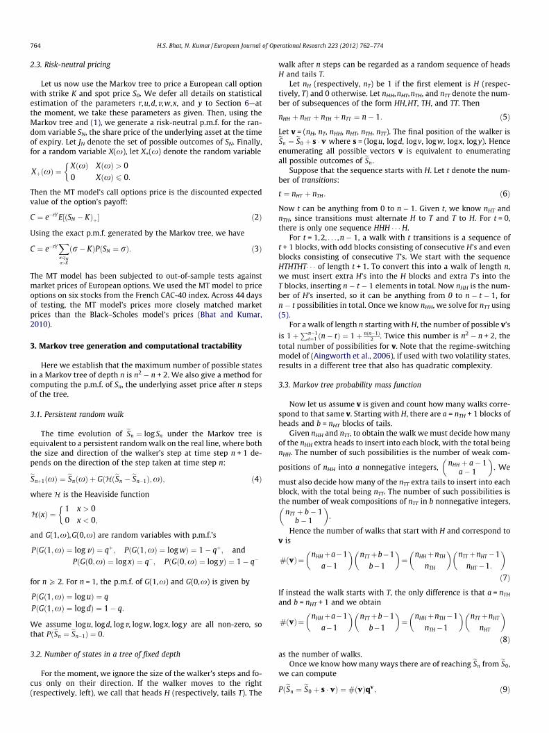
Fig. 4. We fit three p.d.f.’s to daily log return time series for GOOG (left) and DF (right). The p.d.f’s are a kernel density estimate (KDE), a mixture of two normals, and a singlenormal. The results show that the mixture of two normals more closely matches the KDE density. See Section 6.2 for more details.

Table 3For each of 10 days of testing, we record the mean of Emodel(h) for each of three models. For the columns with heading ‘‘All Symbols,’’ the mean is taken over all 89 symbols h,while for the columns with heading ‘‘BIC Symbols,’’ the mean is taken over 71 symbols h for which BIC model selection chooses a normal mixture distribution.

All symbols BIC symbols

Black–Scholes MT Naive MT Reg Black–Scholes MT Naive MT Reg

13 June 2011 0.2026 0.1395 0.1267 0.2217 0.1419 0.118614 June 2011 0.2158 0.1394 0.1276 0.2378 0.1433 0.122515 June 2011 0.1839 0.1346 0.1383 0.1988 0.1352 0.127916 June 2011 0.1732 0.1373 0.1327 0.1854 0.1387 0.133117 June 2011 0.1637 0.1411 0.1277 0.1741 0.1435 0.129320 June 2011 0.1947 0.1397 0.1322 0.2110 0.1408 0.129621 June 2011 0.1977 0.1274 0.1214 0.2182 0.1316 0.124222 June 2011 0.1923 0.1294 0.1254 0.2129 0.1349 0.129123 June 2011 0.1830 0.1197 0.1153 0.2017 0.1234 0.115824 June 2011 0.1685 0.1297 0.1348 0.1824 0.1315 0.1300

1 2 3 4 5 6 7 8 9 100.1

0.15

0.2

0.25

Day

Mea

n of

erro

r

B−SMT RegMT Naive

1 2 3 4 5 6 7 8 9 100

0.005

0.01

0.015

0.02

0.025

0.03

0.035

0.04

Day

Varia

nce

of e

rror

B−SMT RegMT Naive

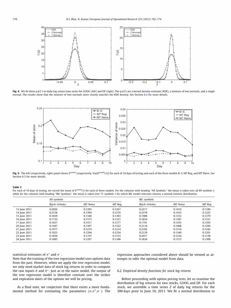
Fig. 5. The left (respectively, right) panel shows Emodel (respectively, Var[Emodel(h)]) for each of 10 days of testing and each of the three models B–S, MT Reg, and MT Naive. SeeSection 6.3 for more details.

770 H.S. Bhat, N. Kumar / European Journal of Operational Research 223 (2012) 762–774

statistical estimates of r+ and r�.Note that the training of the tree regression model uses options datafrom the past. However, when we apply the tree regression model,we only need market data of stock log returns in order to computethe raw inputs r̂ and r̂�. Just as in the naive model, the output ofthe tree regression model is therefore constant over the strikesand expiration dates of the options we will be pricing.

As a final note, we conjecture that there exists a more funda-mental method for estimating the parameters (r,r+,r�). The

regression approaches considered above should be viewed as at-tempts to infer the optimal model from data.

6.2. Empirical density functions for stock log returns

Before proceeding with option pricing tests, let us examine thedistribution of log returns for two stocks, GOOG and DF. For eachstock, we assemble a time series Z of daily log returns for the300 days prior to June 10, 2011. We fit a normal distribution to

Table 4For each of 10 days of testing, we record the variance of Emodel(h) for each of three models. The column headings ‘‘All Symbols’’ and ‘‘BIC Symbols’’ denote the same set of symbolsdescribed in Table 3.

All symbols BIC symbols

Black–Scholes MT Naive MT Reg Black–Scholes MT Naive MT Reg

13 June 2011 0.0188 0.0047 0.0043 0.0208 0.0050 0.003814 June 2011 0.0259 0.0064 0.0036 0.0287 0.0070 0.003015 June 2011 0.0169 0.0049 0.0053 0.0191 0.0052 0.004216 June 2011 0.0162 0.0058 0.0044 0.0188 0.0064 0.004617 June 2011 0.0171 0.0082 0.0051 0.0201 0.0094 0.005620 June 2011 0.0261 0.0079 0.0058 0.0298 0.0085 0.006221 June 2011 0.0226 0.0060 0.0051 0.0251 0.0065 0.005822 June 2011 0.0219 0.0058 0.0062 0.0246 0.0064 0.006823 June 2011 0.0176 0.0036 0.0043 0.0195 0.0039 0.004724 June 2011 0.0126 0.0041 0.0051 0.0142 0.0044 0.0044

0 0.5 10

0.25

0.5

Black−Scholes

Mar

kov

Tree

0 0.5 10

0.25

0.5

Black−ScholesM

arko

v Tr

ee

0 0.5 10

0.25

0.5

Black−Scholes

Mar

kov

Tree

0 0.5 10

0.25

0.5

Black−Scholes

Mar

kov

Tree

0 0.5 10

0.25

0.5

Black−Scholes

Mar

kov

Tree

0 0.5 10

0.25

0.5

Black−Scholes

Mar

kov

Tree

0 0.5 10

0.25

0.5

Black−Scholes

Mar

kov

Tree

0 0.5 10

0.25

0.5

Black−Scholes

Mar

kov

Tree

0 0.5 10

0.25

0.5

Black−Scholes

Mar

kov

Tree

0 0.5 10

0.25

0.5

Black−Scholes

Mar

kov

Tree

Fig. 6. We give 10 scatterplots, one for each day of testing. Each scatterplot has 89 points of the form (EB�S(h), EMT Reg(h)). The majority of the points lie below the line of slopeone. The B–S model’s errors are larger and more dispersed than the MT model’s errors. See Section 6.3 for more details.

H.S. Bhat, N. Kumar / European Journal of Operational Research 223 (2012) 762–774 771

0 0.5 10

0.25

0.5

Black−Scholes

Mar

kov

Tree

0 0.5 10

0.25

0.5

Black−Scholes

Mar

kov

Tree

0 0.5 10

0.25

0.5

Black−Scholes

Mar

kov

Tree

0 0.5 10

0.25

0.5

Black−Scholes

Mar

kov

Tree

0 0.5 10

0.25

0.5

Black−Scholes

Mar

kov

Tree

0 0.5 10

0.25

0.5

Black−Scholes

Mar

kov

Tree

0 0.5 10

0.25

0.5

Black−Scholes

Mar

kov

Tree

0 0.5 10

0.25

0.5

Black−Scholes

Mar

kov

Tree

0 0.5 10

0.25

0.5

Black−Scholes

Mar

kov

Tree

0 0.5 10

0.25

0.5

Black−Scholes

Mar

kov

Tree

Fig. 7. We give 10 scatterplots, one for each day of testing. Each scatterplot has 89 points of the form (EB�S(h), EMT Naive(h)). The majority of the points lie below the line ofslope one. The B–S model’s errors are larger and more dispersed than the MT model’s errors. See Section 6.3 for more details.

772 H.S. Bhat, N. Kumar / European Journal of Operational Research 223 (2012) 762–774

the time series using the sample mean and variance of Z. We alsoapply the Expectation Maximization (EM) algorithm to fit a mix-ture of two normals to Z. Finally, we use kernel density estimation(KDE) to fit a density f(z) to Z.

In Fig. 4, we plot the three densities for GOOG (respectively, DF)in the left (respectively, right) panel. For GOOG, the mixture of twonormals fits the KDE density better than the single normal, espe-cially at the peak of the distribution and the region near the peak.For DF, the agreement between the KDE density and the mixture oftwo normals is even more pronounced. The single normal does notfit nearly as well.

We conclude that, at least for these two stocks, the mixture oftwo normal distributions fits much better than a single normal.We test this for all stocks in the following way. For each stock,we take the time series of daily log returns and fit (i) a single

normal and (ii) a mixture of two normals. After fitting, we calculatethe BIC-penalized likelihood for both (i) and (ii). The BIC penaltyterm accounts for the fact that the mixture has five parameters in-stead of just two parameters for the single normal.

We find that for 71 out of the 89 total stocks, the BIC-penalizedlikelihood is larger for the normal mixture distribution. From amodel selection point of view, this indicates that the normal mix-ture is a better choice for modeling log return time series.

6.3. Comparing model and market option prices

We now test the models MT Naive and MT Reg, introduced inSection 6.1, against both Black–Scholes model prices and marketprices of options. We collected from Yahoo! Finance 11 days ofmarket prices for options on 89 non-dividend-paying stocks from

H.S. Bhat, N. Kumar / European Journal of Operational Research 223 (2012) 762–774 773

the S&P 500. In what follows, we refer to the average of the bid andask prices as the market price of the option.

For MT Reg, the previous day’s option prices are required totrain the model. Hence with 11 days of options data, we can makea fair comparison between model and market prices for the final10 days. For these same 10 days, we also compute option pricesusing the MT Naive and the Black–Scholes models.

Here is how we compute the error on each day. Suppose wehave fixed the stock symbol h and we focus on one particular expi-ration date s. Then there will be call options at, say, k differentstrikes; let Cmarket, a vector of length k, denote the market pricesof these call options. We compute the mean of the absolute valuesof the relative errors between market and model prices:

Emodelðh; sÞ ¼ 1k

Xk

i¼1

Cmarketi � Cmodel

i

Cmarketi

����������;

where ‘‘model’’ can take the values B–S (Black–Scholes), MT Reg, orMT Naive. We choose this metric because we are concerned withthe percentage errors made in pricing each option that is traded.Other error metrics, such as RMS absolute error in units of dollars,assign lower importance to mispricing options that are worth less.

We then average Emodel(h,s) over all possible expirations s to ob-tain the mean error Emodel(h) committed by the model for the sym-bol h. Finally, we average over all symbols h to obtain the meanerror Emodel committed by the model. Through all of this, E hasthe units of fractional error, i.e., 100 E has units of percentageerror.

In the left panel of Fig. 5, we plot Emodel for each of the 10 days oftesting, and for each of the three models. The values that are plot-ted are also given in Table 3 under the heading ‘‘All Symbols.’’ Thevalues that are plotted under the heading ‘‘BIC Symbols’’ are aver-ages of Emodel(h) over those 71 symbols h for which BIC selects anormal mixture distribution for the log return time series—see Sec-tion 6.2 for more details.

In the right panel of Fig. 5, we plot the variance Var[Emodel(h)]for each of the 10 days of testing, and for each of the three models.The values that are plotted are also given in Table 4 under theheading ‘‘All Symbols.’’ The values that are plotted under the head-ing ‘‘BIC Symbols’’ are variances Var[Emodel(h)] over those 71 sym-bols h for which BIC selects a normal mixture distribution for thelog return time series.

Fig. 5 shows that both the mean and the variance of the MTmodel’s errors are less than the B–S model’s errors over all 10 daysof testing. The small and nearly constant variance of the MT mod-el’s errors hints that the method is robust and would fare well overa much longer period of testing. In future work, we intend to pur-sue exactly such a test.

Tables 3 and 4 also show that, across all days of testing, the MTmodels perform better than the B–S model. Additionally, we seethat using the MT models for symbols for which BIC model selec-tion selects a single normal density does not incur any special pen-alty. However, if one examines the B–S columns in these tables,one finds that the B–S model does perform noticeably worse onsymbols for which BIC model selection chooses a mixture model.

Another visualization of the errors committed by the MT Regmodel is provided in Fig. 6. Here we have 10 scatterplots, one foreach day of testing. Each scatterplot has 89 points of the form(EB�S(h),EMT Reg(h)). On all of the scatterplots, the vertical axis hasbeen truncated at 0.5, which is sufficient to contain all the points.The horizontal axis has twice the range to account for the errorsmade by the B–S model. Clearly, the errors made by the MT Regmodel are much less dispersed in space than those made by theB–S model. We plot a line of slope one to show that the majorityof the 89 points lies below the line, i.e., the MT Reg model’s erroris less than the B–S model’s error for the majority of symbols h.

The same type of visualization of errors for the MT Naive modelis provided in Fig. 7. Again we have 10 scatterplots, one for eachday of testing. Each scatterplot has 89 points of the form (EB�S(h),EMT Naive(h)). The performance of the MT Naive model is not quiteas sharp as the MT Reg model, but the same general conclusionsfrom the previous paragraph apply.

Appendix A. Expressions for normal mixture distributionparameters

We list expressions for the constants l1,r1,l2, and r2 that ap-pear in the normal mixture distribution (27).

l1 ¼ eS0 � lu þl1ðqþ � 1Þðq� þ qþÞ þ l2ðq�ðq� � 3qþ þ 3Þ þ qþ � 1Þ

ðq� � qþ þ 1Þ2

þ ðn� 1Þðl1q�ð1� 2qþÞ þ l2ð2q� � 1Þðqþ � 1ÞÞq� � qþ þ 1

r21 ¼ �ðn� 1Þq�ðqþ � 1Þ qþ l2

1ð4q�ðq� þ 2Þ � 3Þ�h

� 2l1l2ð4q�ðq� þ 2Þ � 9Þ þ l22ð4q�ðq� þ 2Þ � 11Þ

�� 4ðq� � 1Þqþ2ðl1 � l2Þ2 � ðq� � 1Þðl1 � 3l2Þ2

iðq� � qþ þ 1Þ�3

� ðqþ � 1Þ l21 q�3 þ q�2ð2qþ � 1Þ þ q�ðqþð9qþ � 8Þ þ 1Þ�h

þ qþ � 1Þqþð Þ � 2l1l2 q�3 þ q�2ð6qþ � 5Þ þ q�ð5ðqþ � 2Þqþ þ 3Þ�

� qþ2 þ qþ�þ l22 q�3 þ q�2ð10qþ � 13Þ þ q�ððqþ � 12Þqþ þ 13Þ

�þ qþ � 1Þqþð Þ�ðq� � qþ þ 1Þ�4

l2 ¼ eS0 þ lu þl1 q�ð3qþ � 2Þ � ðqþ � 1Þ2� �

� l2q�ðq� þ qþ � 2Þ

ðq� � qþ þ 1Þ2

þ ðn� 1Þðl1q�ð1� 2qþÞ þ l2ð2q� � 1Þðqþ � 1ÞÞq� � qþ þ 1

r22 ¼�ðn�1Þq�ðqþ �1Þ qþ l21ð4q�ðq� þ2Þ�3Þ

�h� 2l1l2ð4q�ðq� þ2Þ�9Þþ l2

2ð4q�ðq� þ2Þ�11Þ�

� 4ðq� �1Þqþ2ðl1� l2Þ2�ðq� �1Þðl1�3l2Þ2iðq� �qþ þ1Þ�3

� q� l21 q�2ðqþ �2Þþq�ð10ðqþ �1Þqþ þ1Þþqþ3�qþ� �h

� 2l1l2 q�2ð5qþ �4Þþq�ð6ðqþ �2Þqþ þ5Þþ ðqþ �3Þðqþ �1Þqþ� �

þ l22 q�2ð9qþ �10Þþq�ð2ðqþ �7Þqþ þ13Þ�

þ qþ �1Þððqþ �3Þqþ þ4Þð Þ�ðq� �qþ þ1Þ�4:

References

Aingworth, D.D., Das, S.R., Motwani, R., 2006. A simple approach for pricing equityoptions with Markov switching state variables. Quantitative Finance 6 (2), :95–105.

Appleby, J.A.D., Daniels, J.A., Krol, K., 2012a. A Black–Scholes model with longmemory.

Appleby, J.A.D., Riedle, M., Swords, C., 2012b. Bubbles and crashes in a Black-Scholesmodel with delay. Finance and Stochastics.

Arriojas, M., Hu, Y., Mohammed, S.-E., Pap, G., 2007. A delayed Black and Scholesformula. Stochastic Analysis and Applications 25 (2), :471–492.

Barone-Adesi, G., 1985. Arbitrage equilibrium with skewed asset returns. Journal ofFinancial and Quantitative Analysis 20 (3), 299–313.

Basu, A., Ghosh, M.K., 2009. Asymptotic analysis of option pricing in a Markovmodulated market. Operations Research Letters 37 (6), :415–419.

Behr, A., Pötter, U., 2009. Alternatives to the normal model of stock returns:Gaussian mixture, generalised logF and generalised hyperbolic models. Annalsof Finance 5 (1), 49–68.

Bhat, H.S., Kumar, N., 2010. Markov tree options pricing. In: Proceedings of theFourth SIAM Conference on Mathematics for Industry (MI09), San Francisco, CA,pp. 162–173.

774 H.S. Bhat, N. Kumar / European Journal of Operational Research 223 (2012) 762–774

Bouchaud, J.P., Potters, M., 2003. Theory of Financial Risk and Derivative Pricing:From Statistical Physics to Risk Management. Cambridge University Press.

Breiman, L., Friedman, J.H., Olshen, R.A., Stone, C.J., 1984. Classification andRegression Trees. Wadsworth Statistics/Probability Series. WadsworthAdvanced Books and Software, Belmont, CA.

Brigo, D., Mercurio, F., 2002. Lognormal-mixture dynamics and calibration tomarket volatility smiles. International Journal of Theoretical and AppliedFinance 5 (4), :427–446.

Buckley, I., Saunders, D., Seco, L., 2008. Portfolio optimization when asset returnshave the Gaussian mixture distribution. European Journal of OperationalResearch 185 (3), :1434–1461.

Cai, N., Kou, S.G., 2011. Option pricing under a mixed-exponential jump diffusionmodel. Management Science 57 (11), :2067–2081.

Camara, A., Li, W., 2008. Jump-Diffusion Option Pricing without IID Jumps. SSRNeLibrary.

Campbell, J.Y., Lo, A.W.C., MacKinlay, A.C., 1997. The Econometrics of FinancialMarkets. Princeton University Press.

Chang, M.-H., Pang, T., Pemy, M., 2010. An approximation scheme for Black–Scholesequations with delays. Journal of Systems Science and Complexity 23 (3), 438–455.

Chang, M.-H., Pang, T., Yang, Y.P., 2011. A stochastic portfolio optimizationmodel with bounded memory. Mathematics of Operations Research 36 (4),604–619.

Chang, M.-H., Youree, R.K., 2007. Infinite-dimensional Black–Scholes equationwith hereditary structure. Applied Mathematics and Optimization 56 (3),395–424.

Cont, R., 2001. Empirical properties of asset returns: stylized facts and statisticalissues. Quantitative Finance 1 (2), 223–236.

D’Amico, G., Janssen, J., Manca, R., 2009. European and American options: the semi-Markov case. Physica A 388 (15–16), 3181–3194.

Ding, Z., Granger, C.W.J., Engle, R.F., 1993. A long memory property of stock marketreturns and a new model. Journal of Empirical Finance 1 (1), 83–106.

Eberlein, E., Keller, U., 1995. Hyperbolic distributions in finance. Bernoulli 1 (3),281–299.

Fama, E.F., 1970. Efficient capital markets—a review of theory and empirical work.Journal of Finance 25 (2), 383–423.

Fielitz, B.D., 1975. On the stationarity of transition probability matrices of commonstocks. The Journal of Financial and Quantitative Analysis 10 (2), 327–339.

Fielitz, B.D., Bhargava, T.N., 1973. The behavior of stock-price relatives—aMarkovian analysis. Operations Research 21 (6), 1183–1199.

Heston, S.L., 1993. A closed-form solution for options with stochastic volatility withapplications to bond and currency options. Review of Financial Studies 6 (2),327–343.

Heston, S.L., Nandi, S., 2000. A closed-form GARCH option valuation model. TheReview of Financial Studies 13 (3), 585–625.

Hull, J.C., 2009. Options, Futures and Other Derivatives. Prentice Hall finance series,Prentice Hall.

Inverarity, G.W., 2003. Numerically inverting a class of singular Fourier transforms:theory and application to mountain waves. Proceedings of the Royal Society ofLondon Series A – Mathematical Physical and Engineering Sciences 459 (2033),1153–1170.

Jackwerth, J.C., 1999. Option implied risk-neutral distributions and impliedbinomial trees: a literature review. Journal of Derivatives, 66–82.

Janssen, J., Manca, R., Biase, G.D., 1997. Markov and semi-Markov option pricingmodels with arbitrage possibility. Applied Stochastic Models and Data Analysis13, 103–113.

Kazmerchuk, Y., Swishchuk, A., Wu, J., 2007. The pricing of options for securitiesmarkets with delayed response. Mathematics and Computers in Simulation 75,69–79.

Kendall, M.G., 1944. The Advanced Theory of Statistics. I.J.B. Lippincott Co.,Philadelphia.

Kon, S.J., 1984. Models of stock returns—a comparison. Journal of Finance 39 (1),147–165.

Lighthill, M., 1958. Introduction to Fourier Analysis and Generalised Functions.Cambridge Monographs on Mechanics and Applied Mathematics. CambridgeUniversity Press.

Longin, F., 2005. The choice of the distribution of asset returns: how extreme valuetheory can help? Journal of Banking & Finance 29 (4), 1017–1035.

Mamon, R.S., Rodrigo, M.R., 2005. Explicit solutions to European options in aregime-switching economy. Operations Research Letters 33 (6), 581–586.

Nelder, J.A., Mead, R., 1965. A simplex method for function minimization. TheComputer Journal 7 (4), 308–313.

Niederhoffer, V., Osborne, M.F.M., 1966. Market making and reversal on the stockexchange. Journal of the American Statistical Association 61 (316), 897–916.

Ramponi, A., 2011. Mixture dynamics and regime switching diffusions withapplication to option pricing. Methodology and Computing in AppliedProbability 13 (2), 349–368.

Ritchey, R.J., 1990. Call option valuation for discrete normal mixtures. Journal ofFinancial Research 13 (4), 285–296.

Rudnick, J.A., Gaspari, G.D., 2004. Elements of the Random Walk: An Introductionfor Advanced Students and Researchers. Cambridge University Press.

Sewell, M., 2011. Characterization of financial time series. Technical Report RN/11/01, University College London, London.

Shreve, S.E., 2004. Stochastic Calculus for Finance. I. Springer Finance. Springer-Verlag, New York.

Swords, C., Appleby, J.A.D., 2010. Stochastic Delay Difference and DifferentialEquations. Lambert Academic Publishing.

Tan, K., Chu, M., 2012. Estimation of portfolio return and value at risk using a classof Gaussian mixture distributions. The International Journal of Business andFinance Research 6 (1), 97–107.

Taylor, S.J., 2007. Introduction to Asset Price Dynamics. Volatility, and Prediction.Princeton University Press.

Wu M., Huang N., Zhao, C., 2008. European option pricing with time delay. In 2008Chinese Control Conference (CCC). IEEE, Piscataway, NJ, USA, pp. 589–593.