REPORT OF THE COMPTROLLER GENERAL OF THE UNITED STATES lllllllillllllllillllllllilll~lll~ LMO99406 Grain Reserves: A Potential U.S. Food Policy Tool GAO, in considering grain reserves as part of U.S. food policy, concludes that: --We cannot be certain that adverse weather -shocks, similar to those in 1972 and 1974, will not occur in the future. Such shocks would tax existing food supplies and the United States would be faced with making decisions on domestic price increases and alloca- tions of food abroad. -- 2 --Rather than face these future decisions as crisis decisions, a grain reserve that is built during years of plenty and made available during lean years could act as a buffer against unpredictable shocks to the food system. --Because a food reserve would be a physical source of food, it deserves seri- ous attention by the Congress as part of a package to meet US. food policy objectives. OSP-76-16 8;4ARCH26,1976
Transcript
REPORT OF THE COMPTROLLER GENERAL OF THE UNITED STATES
GAO, in considering grain reserves as part of U.S. food policy, concludes that:
--We cannot be certain that adverse weather -shocks, similar to those in 1972 and 1974, will not occur in the future. Such shocks would tax existing food supplies and the United States would be faced with making decisions on domestic price increases and alloca- tions of food abroad.
-- 2
--Rather than face these future decisions as crisis decisions, a grain reserve that is built during years of plenty and made available during lean years could act as a buffer against unpredictable shocks to the food system.
--Because a food reserve would be a physical source of food, it deserves seri- ous attention by the Congress as part of a package to meet US. food policy objectives.
OSP-76-16 8;4ARCH26,1976
COMPTROLLER GENERAL OF THE UNWED STATES
WASHINGTON. D.C. 20548
B-114824
The Honorable George McGovern , Chairman, Select Committee on
Nutrition and Human Needs United States Senate
Dear Mr. Chairman :
This report addresses the issue of grain re- serves as requested in your August 7, 1975, letter.
The report provides a perspective on agricul- tural policy, on the newly emerging uncertainty that U.S. grain production can adequately satisfy food needs, and on the factors that need considera- tion in developing a grain reserve program as part of food policy.
The body of the report together with the appen- dices provides a summary of grain reserve resea
Comptroller General of the United States
Contents ---.--
Page ---
DIGEST i
CHAPTER
I INTRODUCTION
U.S. Grain Stock Programs From Abundance to Uncertainty Why Reserves?
2 AGRICULTURAL POLICY PERSPECTIVE
Traditional Agricultural Policy Goals 8 Farm Income Maintenance 8 Protection of Consumers 12 Agricultural Exports 14
3 AN EMERGING GOAL: STABILITY /
New Situation: Uncertainty 17 The Economic Cost of Instability 17 Causes of Market Instability 18 Achieving Market Stability 19
4 RESERVE POLICY FACTORS
Global Versus Domestic Scope 24 Objectives of Stock Management 25 Levels of Reserves 25 - Market Intervention Policy 27 Institutional Control 27 Financing Operations 26
Coordination with Domestic Farm Policy 29 Coordination With Export Control Policy 30 Myths 31
5 CONCLUSIONS
APPENDIX
I REVIEW OF LEGISLATIVE PROPOSALS ON GRAIN RESERVES
II AN ILLUSTRATIVE SIMULATION MODEL FOR RESERVE STOCK MANAGEMENT
III REVIEW OF RESERVE POLICY MODELS
IV RESERVE RESEARCHERS CONTACTED
8
17
23
33
35
44
56
85
V BIBLIOGRAPHY 88
ABBREVIATIONS
ccc
GAO
Commodity Cred'it Corporation
General Accounting Office
COMPTROLLER GENERAL'S REPORT To THE SENATE SELECT COMMITTEE ON NUTRICTION AND HUMAN NEEDS
GRAIN RESERVES: A POTENTIAL U.S. FOOD POLICY TOOL
DIGEST ------
Until recently, the United States' prime agricultural concern was what to do with large crop surpluses which tended to curb farm income. With the massive drawdown of world wide grain surpluses beginning in 1972, this concern shifted to in- clude the additional question of what to do in the case of crop shortages, which tend to decrease food availability and increase consumer prices.
To help satisfy both farmer and consumer needs, a number of attempts including legislative proposals (See app.1) have been made that consider a food reserve policy which could be used as a buffer to physically acquire reserves during times of surplus and distribute them during shortages. (See app. III.)
This report describes the events (See chp. 1) which have resulted in general uncertainty and concern over how to handle either agricultural shortages or surpluses which could occur in any crop year. It provides summary information on grain reserves as a buffer mechanism. (See chap. 3.)
The report concentrates on the potential for domestic food reserve mechanisms administered by the United States. It does not dis- cuss the potential food reserve mechanisms administered inter- nationally-- a question which can not be solved by a U.S. deci- sion alone. Although many types of reserves can be considered, only grain, specifically wheat, is used as an example of food -.a reserves in this report. The report is based on a review of liter- ature and discussions with reserve researchers.
Traditionally, U.S. agricultural policy has had three general . objectives.
--Maintaining the productive base by attempting to stabilize agricultural prices and maintain farmers' incomes.
--Protecting the domestic consumer by attempting to pro- vide adequate supplies at reasonable prices.
--Exporting agricultural surpluses for c<mmercial, humanitarian, and political purposes. :
CA- &de, I-L.5 .mrrTI------r .-
m Sheet, Upon removal. the report cover date should be noted hereon.
._ ,_rC- -
i OSP-76-16
c
For many years the primary agricultural problem was how to cope with overabundance. The allocation of surpluses to competing demands attracted little attention. This resulted in ad hoc decisionmaking when the primary world agricultural problem shifted to one of coping with shortages.
This recent flip-flop of concern over glut and then shortfall and the uncertainty about the future demonstrates the need for flexibility to handle either situation.
Every year there is uncertainty as to whether the U.S. will pro- duce a surplus or shortfall of agricultural goods to satisfy all domestic and foreign demands at reasonable prices. Further- more, there are no fixed criteria for satisfying these various demands under uncertain conditions.
The "problem" under surplus or shortfall conditions is one of distribution rather than product ion. No matter how much is pro- duced, the probability of exactly matching need with supply is unlikely and someone is faced with too little food or too much food. These problems have been and will continue to be faced by the United States as a major world food supplier.
[In this report, GAO makes two assumptions.
d *;J First, decisionmaking according to preconsidered plans and z criteria is preferable to ad hoc decisionmaking. During
periods of uncertainty such as adverse weather and unex- pected export demand, it would be preferable to have plans for effectively dealing with these conditions.
Second, planning for decisions is facilitated if there is a buffer between uncertainities of supply and demand. Therefore, the greater the buffering capability, the greater the likelihood of executing a planned decisionmaking process.
The three objectives cited of U.S. agricultural pol icy tradition- ally have been satisfied in an atmosphere of agricultural surplus. Recent unanticipated shocks to the food system indicate that the future can be characterized by great uncertainties and less sta- bility than experienced in recent decades. It is appropriate to ask whether ad hoc decisionmaking or “crisis management” is desirable.
A system of food reserves,Wti--not-perfect, is a mechanism of increasing predictability for both producers and consumers during periods of agricultural surpluses or scarcities.‘! A reserve system acts as a buffer against major fluctuations in 3Xipply and demand and facilitates establishment of rules for stock accumula- tion and release.
ii .
Since a shortfall of foodstuffs could result in life- Land-death decisions by the United States, additional attention
should be given to developing a food reserves policy to act as a buffer and facilitate decisionmaking in uncertain situations:!
Food Reserve Factors --
Shortages of food tend to increase prices, benefiting farmers and processors at the expense of consumers (domestic and international). Surpluses of food tend to decrease prices and benefit consumers at the expense of farmers. Achieving a balance between the two is a primary issue. (See chapter 4.)
In considering food reserves as a buffer between the food system and unexpected shocks and as a means of balancing pro- ducer and consumer interests, at least eight factors must be examined. (See p. 23.)
1.
2.
3.
4.
5.
6.
7.
8.
What should be the scope of a reserve system (domestic and/or international)? (See p. 24.)
What ought to be the objectives of reserve stock management? (See p. 25.) P
What levels of reserves are appropriate? (See p. 26.)
What ought to be the relationship between the reserve system and the market mechanism? (See p. 26.)
Who ought to control the reserve system? What are the pros and cons of public versus private management? (See p. 28.)
How should reserve financing- operate? Who should bear the costs, how much, and when? (See p. 28.)
What should be the relationship between domestic farm policy and a reserve system, particularly with respect to farm production and farm income? (See p. 29.)
How should the reserve. system be coordinated with export control policy? (See p. 30.)
1
Tear Sheet iii
CHAPTER I ----
INTRODUCTION --- --
This report describes the recent events which have resulted in general uncertainty and concern over how to handle both U.S. agricultural shortages and surpluses whichever would occur in a given crop year. It provides summary information to the Congress on using food reserves as a buffer against major fluctuations in supply and demand. It concentrates on domestic food reserves administered by the United States. It does not discuss potential food reserves mechanisms administered internationally-- since this is a question which can not be solved by a U.S. decision alone. The report is based on a 1975 review of literature and selected discussions with reserve researchers.
Although many types of reserves can be considered (grain, feed grain, oils), only grain, specifically wheat, is used as an example of food reserves in this report because it is accept- able for direct human consumption worldwide and is a major U.S. commodity which has been stockpiled in the past.
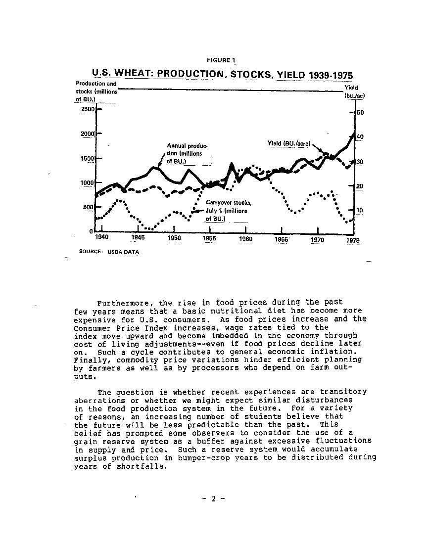
Until recently, with the exception of World War II, there was an apparently adequate supply of grain in worldwide reserves. In 1961, for example , grain reserves had the capability of feeding the world’s population for 95 days. However, in June 1974, the accumulated grain reserves would have fed the world’s population for only 20 days. Since the world has become heavily dependent on North America for its grain supplies, a shortfall in current production could intensify the world’s hand-to-mouth food situation and require U.S. decisions on who gets how much food under what conditions.. Figure 1 provides a comparison of U.S. wheat production, end-of-crop-year carryover stocks, and crop yield, over several decades.
Several factors contributed to this rather sudden reversal from relative abundance to relative scarcity of reserve stocked. Adverse weather conditions in many areas reduced the world harvest by 3 percent in 1972. Weather conditions coincided with the virtual disappearance of Peruvian anchovies which normally contribute a major portion of protein feed for livestock. The reduction of the fishmeal supply dramatically increased the demand for feed grains and protein substitutes.
In addition, the recent energy crisis has imposed a new set of constrictions on the system in the form of fertilizer and pesticide shortages as well as increased transportation costs.
Furthermore, the rise in food prices during the past few years means that a basic nutritional diet has become more expensive for U.S. consumers. As food prices increase and the Consumer Price Index increases, wage rates tied to the index move upward and become imbedded in the economy through cost of living adjustments --even if food prices decline later on. Such a cycle contributes to general economic inflation. Finally, commodity price variations hinder efficient planning by farmers as well as by processors who depend on farm out- puts.
The question is whether recent experiences are transitory aberrations or whether we might expect similar disturbances in the food production system in the future. For a variety of reasons, an increasing number of students believe that the future will be less predictable than the past. This belief has prompted some observers to consider the use of a grain reserve system as a buffer against excessive fluctuations in supply and price. Such a reserve system would accumulate surplus production in bumper-crop years to be distributed during years of shortfalls.
-2-
This idea is certainly not an original one. It dates back to the biblical story of the seven bountiful years and the seven lean years that were ably managed by Joseph in Egypt. Similarly, the policy of maintaining an "ever normal grainery" by buying in years of plenty and selling in years of scarcity was followed in China for more than 1,400 years.
U.S. GRAIN STOCK PROGRAM -m--e ---
The United States has had a policy of publicly-owned accumu- lations of agricultural commodities but it has generally been the indirect result of farm income maintenance programs. The programs attempted to maintain farm incomes and prices and to insure adequate domestic supplies of foodstuffs.
Under the Agricultural Marketing Act of 1929, the Federal - Farm Board was authorized to stabilize farm prices by purchasing surpluses. As Government stocks accumulated, it became apparent that stabilization required both buying and selling. The policy objective of raising farm incomes could only be accomp- lished by reducing agricultural output or by increasing demand.
The Agricultural Adjustment Act was passed in 1933 to increase farmer purchasing power which, for a number of reasons, had declined by 37 percent in the previous 4 years. The objective was accomplished by methods, such as acreage limitations, soil conservation payments, and price supports.
The production adjustments of the Agricultural Adjustment Act were overshadowed by the dramatic increases in technology- induced agricultural productivity, which resulted in excess grain accumulations after World War II. Efforts to dispose elf these surpluses took the form of exports, using subsidies, and giveaways under the Agricultural Trade Development and Assistance Act of 1954 (Public Law 480) and the Food for Peace Act of 1966 (7 U.S.C. 1707a). School lunch and direct commodity distribution programs are examples of domestic uses of farm product surpluses.
FROM GRAIN ABUNDANCE TO UNCERTAINTY ----------
The policies of income maintenance, production restrictions, and surplus disposal were developed over a period of rising agricultural productivity both domestically and internationally. Today, it appears that the era of overproduction and surpluses has come to an end and that a new era, characterized by fluctuations between scarcity and surplus, has begun. The poor world grain harvest of 1972 marked the beginning of the change.
-3-
An active policy of recent administrations was the expansion of foreign markets for U.S. agricultural surplus commodities to earn foreign exchange as well as alleviate the depressing effects of the government stockpiles on farm incomes. An expanded export market developed when the Soviet Union suffered disastrous production shortfalls in 1972. The Soviets radically changed their food policy by deciding to maintain their livestock herd production in spite of the grain shortfalls and by entering the world grain market for feed. The United States found a perfect opportunity to divest it- self of 29 million tons of surplus wheat at a government subsidized price.
The U.S. grain harvest for the 1972 crop year was large enough to support the continued expansion of export markets but failed to provide for the rebuilding of depleted stocks. In 1974 the grain situation mirrored that of 1972. The U.S. wheat yield was considerably lower, although expanded acreage brought production to slightly above the 1973 levels. A very poor U.S. corn crop, combined with widspread drought in the Sahel and India and flooding in Bangladesh, strengthened economic pressures on existing grain inventories in the United States. Wheat prices have since soared and dropped, resulting in uncer- tainty on the part of farmers and consumers as to what future market prices and the availability of food will be.
The 1975 Soviet wheat and feed purchase continues to make the future price and supply outlook for grain uncertain. In 1973 the United States responded to the uncertainties rising from export markets by instituting short supply export controls. The use of export controls highlighted a lack of criteria and a general inability to smoothly administer such ad hoc mechanisms. Disagreement over export controls continues to exist even as the U.S. begins to explore another mechanism, long-term contracts, as a means of responding to uncertainties. The ability of export controls or long-term contracts to mitigate uncertainty remains to be seen. In case of a catastrophe, they merely serve as a means of allocating existing grain supplies.
The long-run supply picture appears to be even less certain than the current situation. The increasing affluence throughout the world can be expected to encourage higher levels of meat consumption. The Soviet decision to buy enormous amounts of feed grain to satisfy their increasing desire for meat is an example of this affluence, This attitude will mean greater demand for feed grains which in turn means more acreage devoted to the two-stage food chain systems (feed grain to animal meats) rather than the one-stage system (direct consumption of grains). While rich nations are exercising their affluence to buy meat, the poorer nations are demanding more food to feed their
-4-
growing populations. At the current annual rate of 2 percent,
the world’s population will almost double to 7 billion in the next 25 years. The current uncertainty about prices and availability of food will continue if population and affluence increase.
There are factors, such as arable land, water, and energy, that might tend to limit the expansion of supply. While there is more arable land available, the cost of bringing it under cultivation may be prohibitive. The new acreage would not be as fertiie as the present farm land, as experiments in the Soviet Union and in Brazil’s tropical forest have demonstrated. Critical shortages may develop in the water supplies required for irrigation. Finally the type of system that has yielded the most productive grain crops is dependent on energy and fossil. fuels for fertilizers, pesticides, and horsepower. If recent pressures on energy supplies cant inue, the U.S. agricultural system may experience limits to its growth.
To help put the future supply of world food into per- spective, the following excerpts are taken from an analysis made by Professor David Pimentel l/ at Cornell University. After considering constraints of water, land and fossil energy, he concludes that:
--Already both energy and land resources limitations make it impossible to feed the present world popu- lation of 4 billion a U.S. diet (69-percent animal protein).
--To hold the per capita protein supply in the year 2000 at 1975 levels will require a 66-percent increase in legumes, a loo-percent increase in other vegetables, and a 75-precent increase ‘in cereals to feed 7 billion people.
WHY RESERVES? -- -
The present and future situation of uncertain grain stocks is an important policy consideration. In terms of meeting the policy goals to maintain farm income, guarantee domestic consumer supplies, and provide exports, an uncertain supply situation has definite implications. A properly managed system of reserve stocks is a policy mechanism that could benefit the entire food system including both producers and consumers by reducing the uncertainty of supply.
------__------
I/ David Pimental et al; “Energy and Land Constraints in Food Protein Production,” Science, November 21, 1975. ---
-5-
The historic instability of agricultural prices illustrated in figure 2 creates an element of uncertainty for the producer. The greater the fluctuations in the prices of farm products, the more difficult the farmers decision regarding the use of productive resources. The overall food system would benefit from reduction in the extreme fluctuations of future prices and more information about that range.
_ FIGURE 2 1
U.S. WHEAT: SEASON AVERAGE PliiC-E ~1~3!&1975 --- Price ($/bd
4
Season Average!
I 1 I I I I I I J 1955:
.- - 1940 1945 1950 1960 1965 1970 T975
SOURCE: USDA DATA I ‘1 -+
I
Of course, food reserves are not the only buffering mechanism that can be used to insure food availability and prices. Export controls were used as crisis tools to temporarily relieve domes- tic commodity shortages during 1973. GAO's report, "US Action Needed to Cope with Commodity Shortages," (Apr. 29, 1974, B-114824) documents that these ad hoc tools caused
-6-
--strong negative foreign react ion,
--legal problems due to broken contracts,
--concern over whether the controls satisfied internat ional trade rules,
--uncertainty as to domestic benefits,
--possible windfall profits, and
--debate over inadequacy of criteria for imposing controls and a continuing debate over the value and limitation of export control use.
More recently, during the summer of 1975, the United States began to develop long-term commodity contracts with the Soviet Union, Japan, and Poland. The effect of these contract developments is yet to be assessed.
In providing a flexible policy to satisfy future food demands , alternative mechanisms, including export controls, long-term contracts, and reserves should be considered. However, it must be pointed out that policy tools, such as export controls or contracts merely allocate currently avail- able supplies of food. They do not provide an additional phys- ical inventory, such as reserves.
- 7-
CHAPTER 2
AGRICULTURAL POLICY PERSPECTIVE -_I_----
TRADITIONAL AGRICULTURAL POLICY GOALS --A--- --
Traditionally, U.S. agricultural policy has had three general objectives.
1. Maintaining the productive -base by attempting to stabilize agricultural pr ices and increase farmers I incomes.
2. Protecting the domestic consumers of agricultural products by attempting to provide adequate supplies at reasonable pr ices.
3. Exporting agricultural surpluses for commercial, ‘humani- tarian, and pol it ical purposes.
In the past, conflicts among these objectives did not receive much attention because the farm sector tended to produce surpluses. There was sufficient production to satisfy perceived commercial as well as humanitarian needs. With the recent transition from surpluses to relative scarcity, goal conflicts have become obvious and a new goal, supply stability, is emerging in response to our uncertainty that production can satisfy needs.
FARM INCOME MAINTENANCE -
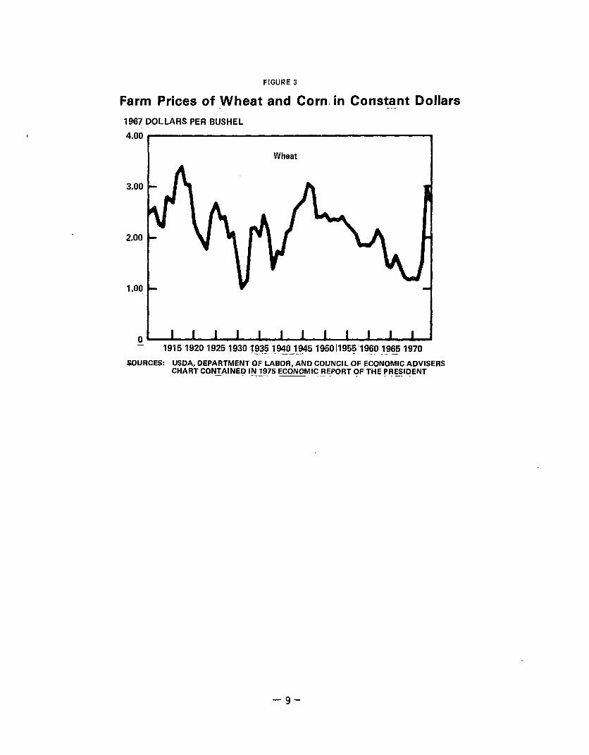
The overriding concern of U.S. agr icultural policy has been the maintenance of farm incomes. During the depression, a series of farm subsidy programs were initiated, and they have been main- tained at various levels over the ensuing years, depending on the volume and prices of farm commodities. During World War II, price ceilings on agricultural commodities were in effect. When these ceilings were lifted after the war, agri- cultural prices rose and subsidies fell to a low of $185 million in 1949. However, the increased productivity and commodity surpluses of the 1950s and 1960s resulted in depressed farm prices. Figure 3 illustrates the downward trend in real prices of wheat from 1948 to 1972. The farmer subsidy programs experi- enced phenomenal growth, reaching $3 billion in 1972, as shown in figure 4. Since 1972, farm prices have risen with a corresponding decrease in subsidy payments.
- 8-
FIGURE 3
Farm Prices of Wheat and Corn1 in Constant Dollars _ . . 1967 DOLLARS PER BUSHEL
b/Includes Great Plains and other conservation programs.
c/Includes all other programs, such as milk indemnity, rental and bene- fits, price adjustment and parity wartime production subsidy, and crop- land adjustment.
d/Less than $0.5 million.
Source: The Economics of Federal Subsidy Programs, Part 7 - Agricultural Subsidies, April 30, 1973, Joint Economic Committee.
-10 - ,,
The combination of price support systems and acreage re- strictions was developed to preserve the family farm as a viable, if heavily subsidized, institution. Another program aimed at preserving the family farm has been the Department of Agriculture’s research and development work which reaches farmers through the agricultural extension offices. While increasing productivity these programs have had the net effect of consolidating and reducing the number of family farms, and continuing the trend toward greater mechanization and more energy-intensive methods of production.
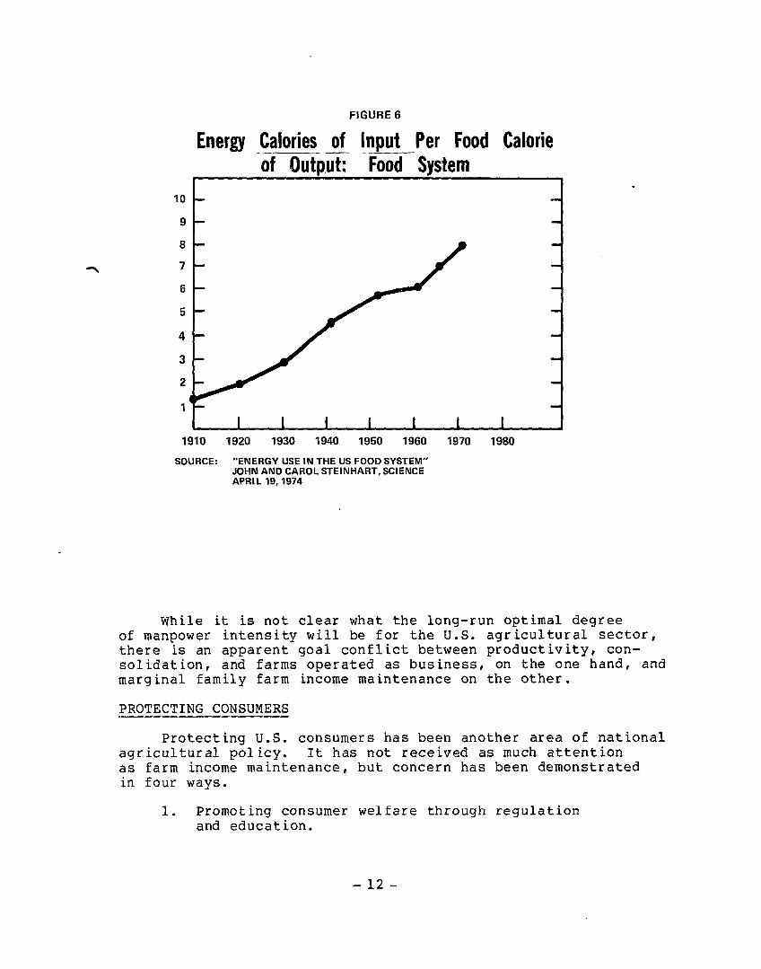
These trends in agriculture can be illustrated. The concentration of production by a few large producers is apparent from the fact that the number of U.S. farms has declined from 5.8 million in 1948 to 2.23 million in 1974. The increased use of machines and their effect on production is shown in figure 5. In 1972 each farmworker produced enough to feed 41 people, compared with only 14 in 1950. The trend in the United States toward a more energy-intensive food system is illustrated in figure 6. The number of energy calories inputs required to produce just one food calorie has grown from about 1 in 1910 to about 8 in 1970.
FIGURE 5
People Supplied Farm Produets Per Farmer, 1950-1972
PEOPLE/FARM WORKER --.
40
25
Carrying Capacity of the Farmer
1950 1955 1960 1965 1970 1975
SOURCE:- “AGRICULTURAL PRODUCTION EiklENCY”,i.iATURAL ACADEMY OF SCIENCES, 1975
- ll-
FIGURE6
Energy Calories of Input Per Food Calorie -_ -if Output: Food System
10 -
9-
8-
7-
6-
5-
4-
I
1910 1920 1930 1940 1950 1960 1970 1980
SOURCE: “ENERGY USE IN THE US FOOD SYSTEM” JOHN AND CAROL STEINHART, SCIENCE APRIL 19,1974
While it is not clear what the long-run optimal degree of manpower intensity will be for the U.S. agricultural sector, there is an apparent goal conflict between productivity, con- solidation, and farms operated as business, on the one hand, and marginal family farm income maintenance on the other.
PROTECTING CONSUMERS ----
Protecting U.S. consumers has been another area of national agricultural policy. It has not received as much attention as farm income maintenance, but concern has been demonstrated in four ways.
1. Promoting consumer welfare through regulation and education.
- 12 -
2.
3.
4.
The
Issuing standards for minimal levels of consumption with adequate nutritional content through social welfare legislation.
Contributing to the development of more nutritionally efficient foods, such as high protein cereal by sponsoring agricultural research.
Helping low-income consumers obtain adequate food through direct commodity distribution and the subsidies of the food stamp program.
fourth area of increasing consumer access of food indicates a goal conflict. While the provisions of low-cost food fb consumers has not been an explicit goal of U.S. agri- cultural pol icy, it certainly is of great importance to consumers. It is of more concern today after the rapid rise in food prices than in recent years. Yet over the years most food legislation has been directed toward supporting agricultural prices. The only exceptions are the system of price ceiling and rationing that were instituted in response to the scarcity situation of World War II, and the recent price freeze administered by the Cost of Living Council. Policies that support farm prices at the expense of the taxpayer and consumer are often defended by the fact that American consumers spend a very small percentage of their income on food. Figure 7 compares an index of personal disposable income with one of food expenditures and also shows food expenditures as a percentage of income.
There has been a steady decline in the food share of income from 1947 to 1972; this has changed recently and food expenditures as percentage of income has increased. There remains the inherent conflict between higher agricultural prices benefiting producers and lower prices benefiting consumers. U.S. agricultural policy h,as tended to resolve this conflict by employing a combination of price supports and subsidies for producers and subsidies (food stamps) for low-income consumers, leaving the taxpayer to pay the bill,
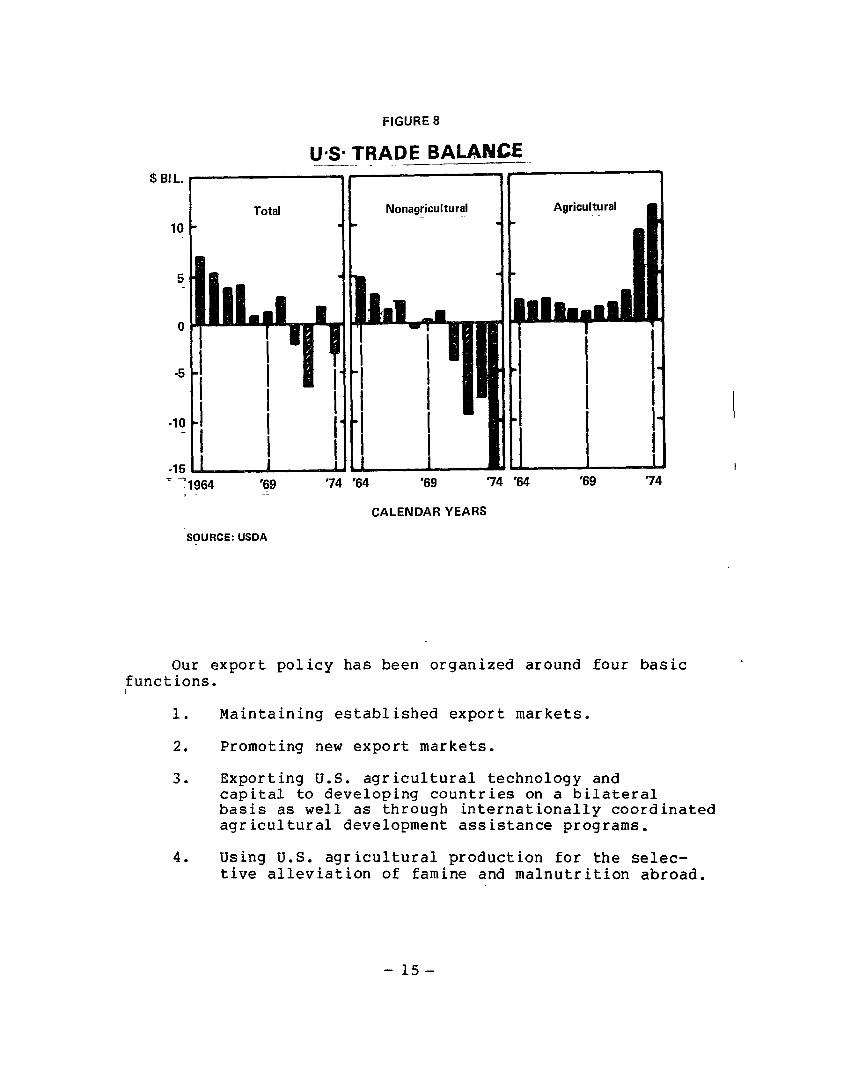
The third traditional goal of U.S. agricultural policy has been developing export markets. The importance of this area is evident from the fact that from 1962 to 1972 the United States exported more than 20 percent of its total crop production. Economically, using our comparative advantage in food production would do much to solve the balance of trade problems that have grown out of recent energy price increases. Figure 8 indicates the important contribution the agricultural sector has been making toward offsetting the recent trade deficits we have been experiencing in the nonagricultural sector. Indeed, in fiscal year 1975, the value of the U.S. agricultural exports reached a new record of $21.6 billion.
- 14 -
$ BIL.
10
5
0
-5
-10
-15
7 Total Nonagricultural Agricultural I
?I964 '69 ‘74 ‘64 ‘69 ‘74 ‘64 ‘69 74
CALENDAR YEARS
‘SOURCE: USOA
FIGURE 8
U+ TRADE BALAWCE -__-. _ .- -
Our export policy has been organized around four basic functions.
1. Maintaining established export markets.
2. Promoting new export markets.
3. Exporting U.S. agricultural technology and capital to developing countries on a bilateral basis as well as through internationally coordinated agricultural development assistance programs.
4. Using U.S. agricultural production for the selec- tive alleviation of famine and malnutrition abroad.
-15-
To some extent, the goal of developing new export markets has conflicted with the humanitarian concern of emergency and famine relief. For instance, the Soviet grain deal in 1972 and its effect on food prices in 1973 and 1974 made it difficult for the United States to promise relief aid at the 1974 World Food Conference, Rome, Italy, because of concern that such aid would cause further domestic price increases.
A graphic illustration of this conflict between commercial and humanitarian concerns can be seen by comparing the two charts in figure 9. Although the dollar value of grain shipments under aid programs has remained almost constant, the physical volume of those shipments has been cut in half between 1969 to 1974--the period during which our commercial exports have grown so rapidly. This goal causes disagreement between the Departments of State and Agriculture over us.ing U.S. production for emergency relief. Precise policy formulation is needed to achieve a balance in the choice between food as trade or aid.
FiGURE 9
U.S. EXPORTS UNDER PUBLIC LAW 480 INCLUDING AID SHIPMENTS
B’L- DoL-YnLUEOF l-
TOTAL SHIPMENTS
2
SOURCE: USDA
MIL. METRiC
I TONS-----l
GRAIN SHIPMENTS
i9S9 ‘70 ‘71 ‘72 ‘73 ‘74 ‘75
-16-
CHAPTER 3
AN EMERGING GOAL: STABILITY -- ------
NEW SITUATION: UNCERTAINTY
With the transition from surpluses to relative scarcity and even shortages that the U.S. and the world have experienced in the recent past, the conflicts among the different agricultural policy objectives have become more obvious. Although the shortage situation is not necessarily a permanent one, there are reasons to believe that it may be since the basic imputs to agriculture, land, water, and energy have worldwide limits. Whether the recent shortage situation is permanent or temporary, it has introduced a new sense of uncertainty not only about future farm policy, but even about the structure of the U.S. food system and its ability to satisfy consumers with reasonably priced products.
THE ECONOMIC COST OF INSTABILITY - .w
The tight supply situation that has developed recently in grain markets may be only a short term situation that will dis- I appear after a few harvests. A more important situation is market instability-- the inability of market supplies to satisfy, at any one time, market needs at reasonable prices. Fluctuations between relatively abundant and relatively scarce supplies of basic grain commodities create price, production, and consumption instability with harmful effects for the food system.
Most grain consumption in the United States takes place indirectly through livestock production. Grain market instability constitutes an important destabilizing effect on agricultural * livestock markets. Extremely high grain prices can cause livestock and dairy producers to reduce their breeding and young stock; which can result in higher production costs and eventually less meat and higher prices for consumers.
Not only does grain market instability affect grain users, but it also disturbs the markets that supply agricultrual inputs, such as the farm equipment and fertilizer industries. Thus, uncertainty can lead to booms and busts in equipment sales, which ripple throughout the nonfarm industrial sector of the domestic economy.
The market for farmland can also be adversely affected by agricultural instability. Boom periods for farmers may increase land values as the farmers' demand for more acreage increases.
-17 -
When commodity prices fall, the acreage expansion plans may be aborted, but land values may not necessarily decline. This phenomenon is often termed the “crop-price ratchet effect” on land values.
Finally, a similar ratchet effect seems to exist between agricultural commodity prices and wages leading to permanently higher prices. Food prices may rise dramatically (as in 1973) creating wage increase demands. Wage increases become imbedded in the economy even after food prices decline, thereby rippling infla- tion throughout other sectors of the economy. In addition, food prices .can increase permanently. If grain prices rise due to real economic pressures, such as bad weather, then higher prices remain imbedded in the profit margins of processors and distributors even after supplies return to normal. The downturn in prices would then be less than what free market economic forces would imply.
While instability inherently has these adverse effects, moderate price variations perform a useful economic function by weeding out inefficient farmers and causing consumers to buy substitute products.
Thus there are arguments for price fluctuation within a tolerable range to reduce the uncertainty of wide fluctuations. Unforeseeable variations in crop yield and export demand will occur, but the reprecussions can be buffered by effective food policy. A policy of grain reserves would control instability and protect consumers and producers from uncertain excessive fluctuations.
CAUSES OF MARKET INSTABILITY
Destabilizing influences exist in the U.S. agricultural product ion and consumption system. Fluctuations occur because of unpredictable shocks to product ion. The most obvious factor affecting production is weather unpredictability with corresponding yield fluctuations.
We also face uncertainty in export demands due to our diffi- culty in forecasting three type of actions.
1. Regular customers may have a particularly good or bad harvest, varying their import demand.
2. There may be irregular customer intervention illustrated by the Soviet entry into the U.S. market in 1972 and again in the summer of 1975. Such irregular interventions may completely disrupt our export distributions and inventor ies.
- 18-
3. Emergency aid requirements transcend the usual economic pressures governing export control and subsidy policies and, therefore, are not mitigated by higher prices.
Unpredicatable weather and export demand influences avail- able supplies and has a secondary impact of altering the supply- demand cycle in following years. Farmers form their production plans for the coming crop year on the basis of current crop price and expectations for next year's prices, but these decisions do not result in production until the following harvest. Demand for the crop, however, is relatively price inelastic L/ with the effect that agricultural demand stays relatively constant regardless of price changes, and supply varies only after a time delay. This interaction is called a cobweb cycle, a continual process of annual production adjustment, which may or may not converge to satisfy demand. The equilibrium that can be reached at some point is usually disrupted by random export demand and weather shocks, which results in a new round of cyclical oscillations and continued market instability.
ACHIEVING MARKET STABILITY .-
TO counteract the uncertainty of weather, export demand, cyclic production variation, and the resulting supply instability, four general methods of controlling production and distribution I are available: price setting, production controls, export controls, and reserve management.
Price setting
Price setting reduces two sources of variation in a market- ing system: movements along the demand curve and future changes in production capacity. It will not have an effect on unexpected variation in foreign emergency demand and weather-related yariations in yields. Price setting may have three undesirable long-term effects depending on the price level.
1. By eliminating market risk to a great degree, price setting reduces technological innovation.
2. Price controls set too high relative to the market- determined price cause uneconomic production, inventory surplus, and depressed demand. The U.S. loan rate policy in the last 25 years has acted in this manner.
----
lJ Quantity demand varies by a smaller percentage than price.
-19-
3. Controlled prices set too low relative to a market- determined price can cause farmers to let their produc- tion capacity depreciate without replacement. In the long runl a very tight market situation could develop with inadequate inventory management, stockpiling, and exportable surpluses. In such a case, the potential development of productive capacity is lost.
Production controls
Price setting in terms of floors and ceilings may be a viable policy alternative when coordinated with production
. controls. There are two types of production controls, acreage controls (productive capacity) and input controls (intensity). The 1970 set-aside program, amended in 1973, required farmers to remove some of their acreage from active agricultural pro- duction in a marketing year when overproduction was expected. This program was coordinated with loan rate policy (essentially a floor price) by requiring participation in the set-aside program as a condition for participation in loan rate. Production management by acreage controls has traditionally been difficult to monitor a If the farmer does participate in the program, he tends to set aside marginally productive land which has limited impact on total production. If the farmer perceives that crop prices are adequate for him, he may not even participate in the program.
. Intensity control policies have not yet been used as a means
to control production. They might take the form of rationing agricultural inputs, such as pesticides, fertilizers, energy, and machinery. Alternatively, a system of subsidies and excise taxes could be imposed on these inputs. In the long run, in- put controls might encourage conservation of energy and capital, slow fertility depletion of the soil, discourage urbanization of rural farmlands, and diminish the negative environmental impacts of highly mechanized modern agriculture.
Export controls
On the demand side, market stability can be increased by export regulation and control. Export regulating is a relatively unwieldy control process. Short-term crisis decisions affect long-term gains in the world market, disrupt importing plans and practices of regular customers, and slow the develop- ment of new markets. Reliance on export regulation has political ramif ications on U.S. relations with importing countries. U.S. export control actions after the 1972 Soviet buying spree are still the subject of controversy and debate.
- 20 - .
Nevertheless, given a reasonable planning horizon and coordination with price floors and production controls, a clearly articulated export regulation policy for agricultural commodities could prove helpful in reducing export demand uncertainty, Policies, such as the development of long-term contracts with regular customers, the earmarking of some part of production for emergency allocations, the use of export subsidies in times of surplus, and annual negotiations with uncontracted regular and occasional importers, may help produc- tion planning and demand forecasting and thus bring about more stability in export shipments.
Reserve management -
The fourth general method of stabilizing an agricultural commodity market is applying reserve management policies. Inventory management in some form already exists at all distri- bution process levels, but an overall inventory management policy for market stabilization does not exist. Reserve policies may be differentiated with reference to three properties.
1. The stabilization objective which refers to that type of inventory in the grain distribution chain which the policymaker seeks to control.
2. The degree of insulation which defines how inventory management operations are affected and, in turn, affect market pricing processes.
3. Managerial rules which describe how the contents of the inventory are controlled.
Reserve management policy could be part of an integrated program which would include some form of all three of the other stabilization methods discussed previously. The degree of co- ordination with other policies is a primary focus of current proposals (see Apps. I and II.) and depends on the concept of the agricultural commodity market, the policy objective, and the structural changes that may have occurred since 1972.
Consideration of reserve management policies as an alter- native market stabilization mechanism may be justified by three arguments.
1. Inventories of commodities are real, and are not merely rules. They can be distributed where needed.
2. Inventories of reserves can be directly controlled. The manipulation of a physically controlled inventory is a
- 21-
relatively simple procedure compared to controlling acreage utilization of many farmers or negotiating export limits with foreign customers. The United States has experience with inventory management. Some inventory maintenance and turnover practices are already widely accepted by commercial as well as public grain carrying establishments. Pipe1 ine inventories and end-of-crop year carryover inventories are current practice. New operations defining additional reserve management policies could become a similarly accepted practice.
3. Stock management could complement other basic ‘market mechanisms. Information links, such as commodity prices, expected demands, and desired supply are inherent in supply and demand interact ion. Stock management serves as an additional mechanism to match current production and demand. Inventories diminish the effects of seasonality on the availability of adequate supplies. The extra commodities held in a reserve management scheme may be considered as another producing entity while inventory capacity of an empty reserve operates as another demanding customer. The other methods of achieving market stabilization are not as complementary to market mechanisms. Price controls, for instance, sever the most important informational link in the system. Similarly, production controls break the link between current adequacy of supply and planned production capacity. Export controls weaken the information flow from price to export demands.
- 22 -
.
CHAPTER 4 -----1.--
RESERVE POLICY FACTORS _---_- ----------.-----
Although the United States has been fortunate in terms of producing agricultural surpluses for several decades, the events of the last few years have not only depleted these surpluses (Government wheat stocks went from 714 million bushels in 1972 to 19 million bushels in 1974) but have contributed to an increase of approximately 15 percent in domestic food prices during the last 2 years. An important question is whether events which affect the food system, such as the Soviet grain deals, adverse cl imat ic conditions, the collapse of the Peruvian anchovy industry, the energy crisis, and the general economic recession are random in nature. If such events are not totally unanticipated and we expect other serious disturbances to the the normal supply-demand cycle to rise in the future, the United States must consider whether our supply of agricultural outputs can satisfy the demands.
Since our ability to supply the various demands for U.S. agricultural products is uncertain, it is necessary to analyze the situation carefully and establish guidelines for decision- making in times of agricultural surplus or scarcity. To do otherwise commits the United States to a strategem of crisis management that resulted after surplus drawdowns in 1972 and 1974.
The use of food reserves is one method of rationalizing our production with needs and should be seriously considered as part of a policy package. Without some form of physical reserves we have no insurance in case of crop failure and commit ourselves to a hand-to-mouth strategy. There is a con- sensus among grain reserve researchers that there are at least eight factors which researchers have identified and must be reviewed and resolved in considering a reserve mechanism. These factors have been incorporated into various simulation models. (See Apps. II and III.)
1. Global versus domestic scope of a reserve system.
2. Objectives of stock management.
3. Levels of reserves.
4. Market intervention.
5. Institutional control.
- 23 -
6. Financing operations.
7. Coordination with domestic farm policy.
8. Coordination with export policy.
GLOBAL VERSUS DOMESTIC SCOPE --- --------
The first factor is finding the proper relationship of a U.S. grain reserve system to the international community. The desired degree of coordination of a U.S. domestic reserve with international policies for world market stabilization is compli- cated by the uncertain boundaries and interdependent nature of the U.S. domestic market with the world market. We can examine the international implications of a U.S. domestic grain reserve policy from three perspectives.
1.
2.
3.
An insulation pol icy: The reserve system may be used to insulate the U.S. grain market from world market instability.
An umbrella policy: The U.S. reserve may unilaterally attempt to stabilize the entire world grain market.
A partial control policy: A U.S.-controlled grain reserve primarily stabilizes the U.S. domestic market, but also reduces extremely tight world market situations to the extent that U.S. price rises permit and catalyzes interest in grain reserves by other countries.
These three interconnected viewpoints underline the need for a consensus on what degree of insulation from world market pressures is desired.
The World Food Conference in Rome, Italy, highlighted the need for international understanding in establishing grain reserves, but very little consensus has been reached on imple- mentation. Although more international policies may be designed in the future, the issues for global negotiation are unlikely to be settled without independent national leadership taking the first step. Thus, this discussion of reserve policy factors concentrates on an independent national effort which views a domestic grain reserve as a stabilizing mechanism for the U.S. food system and as a means of demonstrating to other countries the reasonableness of choosing a buffer stock strategy rather than a hand-to-mouth food strategy.
- 24 -
OBJECTIVES OF STOCK MANAGEMENT mm------ ---------
Stock management policies can be grouped into four categories.
1. Maintaining minimum pipeline or working stocks. Because of potentially disruptive short-term time lags, stable inven- tories of working stocks are required to maintain the grain distribution process from the producer through the processor to the consumer. These inventories serve to maintain the steady flow of grain. This pipeline reserve already exists for normal operating procedures; commercial grain firms satisfy this function. Flour mills currently are using around 50 million bushels of wheat per month and the United States is exporting about 100 million bushels per month.
2. Maintaining commercially held carryovers. Carryovers generally represent grain stocks on hand at the end of the crop year. Carryover stocks serve to smooth seasonal fluctua- tion so, under normal circumstances, demand and expected production may be stable and roughly equal. This presumes predicatable fluctuations unaffected by random destabilizing shocks. These carryovers are also flow-maintaining inventories, which contribute to the food pipeline inventory. This type of grain reserve exists and operates in grain markets today. In the past 3 years wheat crop carryover ranged from 250 to 440 million bushels on July 1, the start of the wheat crop year.
3. Buffering carryovers from destabilizing shocks. Even if economically justified commercial carryovers are managed so that prices are relatively stable, the market destabilizing influence of weather and unanticipated export demands may be large enough to disturb the smooth flow of grains through the carryover inventory system. A separate inventory in addition Ito the pipeline inventory and commercial carryover would minimize or buffer deviations in stock levels from their market equilibrium levels.
A buffer reserve would complement nearly all sectors of the markets since it is a mechanism familiar to the system. By manipulating the level of the reserve, price fluctuations will be moderated. Prices will be contained within a more restricted range, thereby stabilizing the growth of production capacity, helping maintain consumption in times of uncertain weather conditions, and facilitating supply of unexpected commercial export demand. kesearchers on reserve mechanisms generally assume a buffer reserve acumulation of between 200 to 600 million bushels a crop year. This may or may not be combined with the commercial carryover, objectives.
depending on the reserve
-25 -
4. Meeting unexpected emergency foreign demands. Reserve management need not have market stabilization as its sole objec- tive. An additional inventory could be set aside to satisfy emergency aid requirements. Such a reserve would have market stabilizing effects to the extent that it relieves demand pressure on pipeline inventories and commercial carryovers. Some researchers include this reserve in the buffer reserve mentioned above; others conceptualize this reserve as a percentage of annual food needs.
LEVELS OF RESERVES -
To some extent, traditional stock management objectives and required levels have been analyzed by static economic analysis. This analysis indicated that stocks needed for pipeline distr i- bution requirements appear to be within a range of 50 to 100 million bushels of wheat 0 Adequate seasonal grain inventory management or commercial carryover levels can also be derived by empirical analysis of static supply and demand curves. The actual level of wheat carryover in the last 3 years (between 250 and 440 million bushels) is much smaller than the carryover in- 1971 and 1972, which was 731 and 863 million bushels, respec- tively. But the level of reserves required to buffer commer ical carryovers is not certain. Specific criteria for determining the desired level of buffer stocks would include
1. estimated yield variability and its probability distribution;
2. estimated export variability and its probability distribution; and
3. the degree of final market instability to be allowed as indicated by a specific economic index, such as price, carryover level, farm income, exports, and per capita consumption.
Quantitative and qualitative analyses would likely result in a reserve level expressed as a range rather than as a specific figure. As stated earlier, many reserve researchers conduct their analyses using a range of 200 to 600 million bushels of wheat per crop year.
MARKET INTERVENTION POLICY --
A controversial set of questions on reserve management concerns the rules for operating the reserve in coordination with basic market mechanisms. For instance, farmers are not interested in allowing the reserve to sit on the grain market and depress farm prices as government-controlled stocks have
- 26.-
historically done. It is also unacceptable for a reserve to accumulate stocks continually in order to increase farm incomes without similarly arranging for the sale of those stocks to consumers. The provisions of the market intervention policy must be clear and acceptable to all participants in order for the reserve program to achieve its objective of market stability. Three triter ia of market intervention policy can be identified, (1) degree of control, (2) appropriate market signals, and (3) magnitude of stock transfers.
Degree of control
No reserve mechanism can be expected to function so smoothly as to hold the agricultural market at some specified supply, carryover, demand, and market level. Some pr ice movement is expected and desireable to allow the market room to handle normal supply and demand fluctuations. The reserve would buffer abnormal, unanticipated random shocks to the market. The author- ity to operate the reserve would need to be clearly stated.
Appropriate market signals ------
The choice of a signal for reserve policy intervention is an important decision. Several signals, such as prices, carry- over levels, and production and demand forecasts, can be used to coordinate reserve stock acquisition and sales. The signal selection will be based partially on objectives and partially on the current state of agricultural information and forecasting techniques.
Magnitude of stock transfers ---
The determination of how much stock to transfer is as important as the timing of the transfer. Rules must be developed to guide in reading the signal and deciding on the magnitude of transfer. A critical consideration is the importance of maintaining the reserve inventory at the target level. If exact target levels are maintained, then managerial flexibility is curtailed. On the other hand, if maintaining a target level is unimportant, then stocks may be too easily exhausted.
Market intervention policy will be formulated around the answer to three questions: (1) how much stability is desired? (2) when should intervention occur ? and (3) how much intervention should occur?
- 27-
INSTITUTIONAL-CONTROL --
The question of private versus public control of reserve stocks is another important factor. Realistically, the alter- natives involve only two management entities, the Department of Agriculture (the Commodity Credit Corporation and the Agricultural Stabilization and Conservation Service) or private grain companies. Possibly a completely new Government reserve agency could be considered as the public manager, but ‘since the Department of Agr icutlure already manages agricultural stablization programs, it is the likely candidate.
Public management of grain reserves has four apparent advantages over private control.
1. Public control is in a position to balance competing interests among domestic producers, consumers, and foreign importers.
2. Public control can coordinate grain reserve policies in accordance with other agricultural policies.
3. Public control has greater access to basic data sources for reserve operations.
4. Public control needs no economic incentive to maintain and manage market stabilizing grain inventories.
However, commercial traders have considerable experience in managing grainstocks as they already maintain working stocks or pipe1 ine suppl ies, and they also manage carryovers to smooth seasonal fluctuations in supply. If a public grain reserve system is designed to complement the functions of these private inventor- ies, then the potential exists for providing private firms a role in administering the public stocks.
FINANCING OPERATIONS
There are costs that will be incurred by any grain reserve system which will require adequate financing. One cost is the storage process, and another is the interest expense in financing grain purchases. A third cost is the cost of foregoing alternative investment opportunities.
Storage costs are usually assumed to be 15 cents a bushel according to the Uniform Grain Storage Agreement. The interest rate associated with purchasing the grain will vary with the economy. Many reserve models assume rates of 8 to 10 percent. The amount and price of the grain to be financed depends on
- 28 -
the objectives of the reserve. Some reserve researchers assume that wheat would be purchased at the market price, others believe it would be purchased at the target price or loan rate.
The interest costs associated with time, however, can be partially offset by the rules of operating the reserve. Since the reserve generally would be expected to accumulate stocks during unusually good harvest years and transfer stocks to the market during bad harvest years, it will tend to buy when prices are low and sell when prices are high. This gain could be used to compensate for the interest, storage, and transfer costs.
Even if these capital gains could completely offset variable storage costs, there are fixed costs that must be amortized over the reserve lifetime. If there is a critical storage level below which the reserve is not to be depleted, the cost of maintaining that critical level is fixed. Storage capacity must be constructed, rented, or bought. The cost of storage capacity already owned by the reserve must be included in the fixed costs of a reserve system.
To the extent that the market is stabilized, a reserve program will reduce other agricultural policy costs. A price which is stabilized near the target price will tend to decrease deficiency payments and loan rate expenses. These benefits should also be included in the reserve’s financial management policy.
The financial management of a reservep even on a simplified national scale, is a controversial -question. There is no doubt that a reserve policy will cost someone something, but current research varies widely on costs and reserve assumptions. Storage costs and interest costs are not likely to be completely offset by reserve sales, receipts, and decreases in deficiency payments. The question of who pays these costs! thus, becomes an issue which formal analysis can only serve to point out recipients of net benefits and payers of net costs. The cost of being without food in case of a crisis is something that should also be considered.
COORDINATION WITH DOMESTIC FARM POLICY -~-- ---------e-e
A properly managed grain reserve policy should be coordinated with existing farm production controls and income maintenance programs. Production controls are suited for managing extreme instability: they are not expected to “fine tune” the market towards equilibrium as a reserve policy could. Therefore, the two mechanisms can be designed to complement each other. The incentives for full utilization of acreage capacity during
- 29-
World War II, the Korean War, and the aftermath of the Soviet wheat deal are examples of this gross production adjustment process.
Furthermore, since long-term market equilibrium norms for price, SUPPlY I and demand are relatively uncertain and, in fact, change continuously with population, technology, and production costs, reserve operations cannot be a perfect stabilizing method. In this uncertain climate, supplementary stabilizers, such as production controls can work together with a reserve system.
Since the reserve objective is to act as a buffer between the market and random shockss prices can be expected to be less volatile and, thus, farm incomes can be insulated from sharp deviations. It is important, however, that farm income main- tenance policy not conflict with reserve market stabilization operations. Raising loan rates will tend to increase agricul- tural production. If the loan rates are raised artificially above some desirable long-term equilibrium level, overproduction can result e This overproduction tends to increase reserve finances to the point where no more grain may be purchased and the U.S. is faced with the grain surplus problem of the 1950s and 1960s. To some extent this potential problem can be minimized through product ion controls, but unless the coordination of income maintenance I production controls, and reserve transfers is well defined, long-term market stability might not be achieved.,
COORDINATION WITH EXPORT CONTROL POLICY ---- -_Y
There are four types of export control mechanisms which would require coordination with a reserve policy.
1. Ad hoc export quotas or embargoes on specific commodi- ties during periods of short supply.
2. Export subsidies, such as low-interest loans on exports D
3. Outright food aid as part of international political agreements or in times of emergency abroad.
4. Long-term export agreements.
Export quotas are destabilizing in the long run; they tend to disturb regular export markets and slow the growth of new ones. Export subsidies, however I have been considered important for our commitments in promoting U.S. goods1 fostering economic development abroad, and facilitating agricultural surplus dis- posal. Emergency food aid disturbs ordinary market supply-demand relations but represents an important humanitarian and political commitment of U.S. agricultural and foreign policy. Long-term
‘ - 30 -
agreements have recently been negotiated but our experience is very limited and their effectiveness is uncertain.
Export quotas and embargoes generally have been used for gross adjustments during extraordinary circumstances. They are not expected to become a more refined policy tool for market stabilization. Export subsidies have often been subjected to the charge of "dumping" and as such become less useful. Food aid has become a decreasingly smaller share of our gross exports. The costs versus incurred benefits of subsidies have also become a question. Reserve policy tends to insulate the U.S. domestic market from extraordinary world market pressures and thereby diminished the need for more refined export controls.
The critical level of reserves may be tied to an export control policy. When critical levels of reserves are reached, irregular exports of disruptive size may be cut off and some domestic belt tightening may also be urged. This coorination would still allow emergency shipments and continuation of export subsidies for developing countries. In this way a reserve policy can be used to work together with agricultural export control measures and mitigate any disruption they might cause.
MYTHS ---
There are several myths related to reserve policy imple- mentation which should be mentioned. The first is the assumption that a sizeable grain inventory can be effectively insulated from the domestic market. Insulation means that the reserve inventory will not be considered part of the available supply to the market and will not, therefore, influence market behavior. If there are no transfers of stocks between the reserve and marketable inventories, price behavior will not be influenced by the presence of the reserve. Total grain supply is normally defined as the sum of the current year's production plus the commercial carryover from the previous year. As such, any reserve inventory would also be included in total supply as understood by the market's participants. A well-managed reserve system accumlates and releases grain according to a specified set of operational rules. These rules restrict market intervention by reserve managers. As long as these rules are followed, all market participants anticipate the reserve interventions and discount them from market considerations, thereby influencing market behavior but in a uniform manner.
A second myth concerns the depletion of the reserve. The accumulation of a reserve simply to be held with no rules for release is incomplete and unworkable. A nonrelease reserve presumes that the mere existence of reserves acts as a stabilizer.
- 31-
The point is that reserve levels, even critical or minimal levels, may have to be drawn down in extreme situations.
The third myth concerns the inability to build reserve stocks. However, all that is needed to buildup reserve inven- tory is sufficient time, adequate financing of init ial purchases, available storage capacity and production at full capacity levels. Initial reserve acquisitions at moderate levels need not destabilize grain markets if they are purchased over a mod- erate time span. The problem is reduced to one of proper nroduction coordination and export controls, and is not important to the initial buildup of the reserve system. This assumes, of tour se, no disastrous shortfalls overseas or in the United States and to this extent timing is important,
The final myth concerns the location of the reserve inventories and the availability of storage capacity. This problem is superficial in that the underutilized privately and publicly held storage capacity used to store surplus stocks before the 1972 drawdown still exist.
-1 32 -
CHAPTER 5 -----.--
CONCLUSIONS
U.S. food policy has three primary objectives.
1. Maintain farmers' income.
2. Provide reasonablely priced food to domestic consumers.
3. Provide international customers with agricultural products for commercial, humanitarian, and political purposes.
The United States is in an unpredictable period in which it is uncertain whether each year's crop will result in a short- age or surplus of agricultural products.
The current unpredictability is a unique experience in the United States because the primary agricultural worry since the mid 1940s has been how to cope with a glut of foodstuffs.
It is only after adverse weather in 1972 and 1974 and sub- sequent massive drawdown of surpluses that the we recently became concerned with shortages. As such, the country's decisions on how to handle agricultural shortages since 1973 have been of an ad hoc crisis nature, mainly because the adverse conditions and their consequences were not foreseen and alternative policies were not planned.
Since similar adverse weather shocks can be anticipated to occur in the future with resulting worldwide instability in foodstuff markets, a number of researchers have attempted to conceptualize a food reserve mechanism as part of a policy package to handle food shortfall and surplus situations. Food reserves could improve predictability of market price to the farmer and consumer and also provide a physical supply of food, in contrast to other allocation mechanisms, such as export controls or longterm contracts, which only provide the rules to allocate available supplies.
Since the U.S. and the world is in an uncertain period where shortfalls are as probable as surpluses, additional attention should be given to developing a food reserve mechanism to facilitate decisionmaking and management. Without some form of physical reserve, the U.S. has no insurance in case of crop failure and commits the country and our foreign customers to a hand-to-mouth strategy.
- 33 -
Future research on food reserves as a buffering mechanism must be concerned with the general objective of food policy and with creating a balance of benefits for farmers and consumers al ike. Analysis of the following eight factors as discussed in this report will provide the tools for a working food reserve mechanism.
--Scope of the reserve.
--Objectives of stock management.
--Level of the reserve.
--Interface with the market.
--Control of the reserve.
--F inane ing .
--Interface with domestic farm policy.
--Relationship with export policy.
-34 -
APPENDIX I APPENDIX I
REVIEW OF LEGISLATIVE PROPOSALS
ON
GRAIN RESERVES
- 35 -
APPENDIX I APPENDIX I
BILL: Senate bill 2005.
SESSION: 93d Congress, 2nd session.
SPONSOR: Senator Hubert Humphrey.
STATUS: Reintrohcet3 in 94th Congress on Agriculture and Forestrv
?S S.513 referred to Committee
OBJECTIVE: TO provide for adequate reserves of certain ’ agricultural commodities.
PROVISIONS:
1.
2.
3.
4.
5.
6.
7.
Increases target prices for the 1974-77 crop years.
Sets loan rate at 66-2/3 percent of target price.
Provides for adjustment of target prices beginning in the 1975 crop year.
Specifies new Commodity Credit Corporation (CCC) stock acquisition and release rules.
Specifies critical levels of commodities.
Amends recall provisions for loans.
Establishes export licensing requirements for critical commodities.
TARGET LEVELS: 600 million bushels in total wheat carryovers and 200 million bushels in CCC inventories.
MARKET INTERVENTION POLICY:
1. Trigger signal-- current market price.
2. Instability range allowed, dependent on current carryover levels. CCC is prohibited, except for dispositions under Public Law 480, from selling wheat stocks at less than 135 percent of the target price if such sale would cause the total estimated carryover at the end of the current marketing year to fall below specified critical amounts or if it would reduce the CCC stocks below 200 million bushels. CCC is prohibited from selling wheat stocks at less than the target price when the total estimated carryover is more than the specified critical amount. When stocks are below critical levels, the Secretary of Agriculture is permitted to raise the loan rate to 90 percent of the target price.
- 36-
APPENDIX I APPENDIX I
3. No provision for the magnitude of stock transfers.
INSTITUTIONAL CONTROL: Stocks are held by both the private sector (farmers and grain traders) and CCC. The Secretary of Agriculture is responsible for coordinating the release and loan rate provisions.
FINANCING OPERATIONS: Not discussed. Revenues from stock sales are desired to meet storage costs.
PRODUCTION CONTROL COORDINATION: Not discussed.
EXPORT CONTROL COORDINATION: Critical commodities have ex- port licensing requirements. During shortfalls the Secretary of Agriculture may designate certain commodities as critical commodities pursuant to the export licensing provisions of Senate bill 2005. When the projected carryover stocks fall below the specified critical amount and when the commodity
/
is specified as a critical commodity, CCC would be prohibited, as long as the stocks remain below the specified amount, from selling any of its stocks of the commodity for export ' for less than 120 percent of the commodity's weekly average price. Sales under Public Law 480 would be exempt from this restriction,
- 37 -
APPENDIX I APPENDIX I
BILL: Senate bill 549, title III, Agricultural Commodity Reserve.
SESSION: 94th Congress, 1st session.
SPONSOR: Senator George McGovern.
STATUS: Referred to the Subcommittee on Agricultural Pro- duction, Marketing, and Stabilization, Senate Committee on Agriculture and Forestry.
OBJECTIVE: To provide additional incentives for farmers to produce wheat, feed grains, and cotton; to provide for the purchase of animals and animal food products for use in food relief programs; to provide for the establishment and maintenance of a reserve inventory of wheat, feed grains, cotton, and soybeans; to amend and improve the food stamp program: and to accomplish other things.
TARGET LEVELS: Total carryovers maintained at 500 million bushels of wheat.
MARKET INTERVENTION POLICY:
1. Reserve transfer signals --expected carryover level.
2. Degree of instability allowed--not prescribed.
3. Magnitude of stock transfers--not prescribed.
The Secretary of Agriculture shall begin purchasing any commodity required for the reserve inventory when the com- modity's estimated carryover for the marketing year concerned exceeds the quantity prescribed. The Secretary may offer such commodity for sale at the commodity's current parity price. Sales are limited to the net quantities by which estimated domestic consumption and exports exceed estimated domestic production and imports. Stocks are to be used as part of emergency aid requirements both domestically and internationally.
INSTITUTIONAL CONTROL: U.S. Department of Agriculture and ccc.
FINANCING OPERATIONS: Not discussed.
PRODUCTION CONTROL COORDINATION: Not discussed.
EXPORT CONTROL COORDINATION: Not discussed.
- 38 -
APPENDIX I APPENDIX I
BILL: House bill 1036.
SESSION: 94th Congress, 1st session.
SPONSORS: Representatives Neal Smith and Robert Bergland.
STATUS: Pending in the House Committee on Agriculture.
OBJECTIVE: To authorize the establishment and maintenance of reserve wheat supplies for national security and to pro- tect the domestic consumer against an inadequate supply of such commodities; to maintain and promote foreign trade; to protect producers of such commodities against an unfair loss of income resulting from the establishment of a reserve supply; to assist in marketing such commodities; to insure the availability of commodities to promote world peace and understanding; and to accomplish other things.
MAXIMUM RESERVE INVENTORIES: 300 million bushels of wheat. I
MARKET INTERVENTION POLICY: I
1. Market signal for reserve transfers; price triggers for sales; and quantity triggers for acquisitions. The addition of any quantity of wheat to the re- serve uses the minimum of (a) 80 percent of esti- mated total carryover in excess of normal carryover for marketing year or (b) the amount that the maximum reserve money exceeds the total stocks of such commodity varied by CCC.
The first rule is similar to the Kalbfleisch-Tweeton- Gustafson optimal carryover policy& the second is a maximum reserve constrained. The maximum price the Secretary of Agriculture is allowed to pay is equal to the average price farmers have received for such commodities during the preceeding 5 marketing years. Reserve stock sales are determined by a market price trigger, that is, when the market price is above 150 percent of the commodity's target price or 150 percent of the average market price over the last 5 years.
2. Instability is allowed; the price can fluctuate between the average target price and 150 percent of the average target price.
3. The magnitude of stock transfers is specified for accumulations but not for reserve sales.
511 See Appendix 111~ @age 69
- 39 -
APPENDIX I APPENDIX I
INSTITUTIONAL CONTROL: U.S. Department of Agriculture and ccc.
FINANCING OPERATIONS: Not discussed.
PRODUCTION CONTROL COORDINATION: Not discussed.
EXPORT CONTROL COORDINATION: Not discussed.
-40 -
APPENDIX I APPENDIX I
BILL: Senate bill 513
SPONSORS: Senators Hubert Humphrey, Walter Mondale, and Gale McGee
SESSION: 94th Congress, 1st session
STATUS: Referred to the Subcommittee on Agricultural Pro- duction, Marketing, and Stabilization, Senate Committee on Agriculture and Forestry.
OBJECTIVE: To provide for adjustments in established price and loan levels for certain agricultural commodities, to improve stabilization of farm prices and incomes, to improve the management of certain agricultural commodities during shortages, and to accomplish other things;
PROVISIONS: Essentially the same as Senate bill 2005.
- 41-
APPENDIX I APPENDIX I
BILL: Senate bill 2274.
SESSION: 94th Congress, 1st session.
SPONSOR: Senator Henry Bellmon.
STATUS: Referred to the Senate Committee on Agriculture and Forestry.
OBJECTIVE: To amend the feed grain and wheat programs to insure adequate production of such commodities for both domestic and export needs without depressing their prices and to accomplish other things.
PROVISIONS:
1.
2.
3.
4.
5.
6.
7.
8.
Cereal producers are given an alternative to the usual set-asides, that is, full production with farmers storing part of the grain produced at their own cost.
If this storage alternative is selected, farmers can borrow 80 percent of the cost of producing the stored grain or $1.85 a bushel of feed grain ($2.50 a bushel of wheat), whichever is greater.
The loan has an initial S-year term, renewable ' annually, with interest based on Treasury obliga-
tion rates.
If prices exceed 150 percent of the loan rate, the producer may sell the stored grain and repay the loan.
If prices exceed 200 percent of the loan rate, the Secretary of Agriculture may require the producer to sell the stored grain and repay the loan.
The Secretary of Agriculture may guarantee commer- cial loans made for the construction of storage facilities.
Whenever the quantities stored under this program reach 500 million bushels for feed grains (350 million bushels for wheat), export controls are prohibited except for national security.
CCC is to maintain an emergency human nutrition reserve of up to 100 million bushels.
- 42 -
APPENDIX I APPENDIX I
TARGET LEVELS: No reference to target levels except pro- visions 7 and 8 above.
MARKET INTERVENTION POLICY:
1. Trigger signal --current market prices.
2. Instability allowed--not specified.
3. Magnitude of transfers--not specified. Each pro- ducer has the option of selling the stored grain on the open market when the price is betwee 150 and 200 percent of the loan rate. # If the rice exceeds 200 percent of the loan rate, the Secretary of Agriculture may require loan repayment.
4. The emergency reserve is to be maintained at a fixed level up to 100 million bushels.
INSTITUTIONAL CONTROL: Grain is stored by the private sector (farmers themselves), and the CCC stores an emergency reserve.
FINANCING OPERATIONS: Most costs of the privately held grain would be borne by the producers themselves. The remaining costs, as well as those due to the emergency reserve, would be included in the Federal budget.
PRODUCTION CONTROL COORDINATION: The producer may privately store stocks as a direct alternative to the current set- aside program. The producer stores an amount of grain which corresponds to the acreage not set aside.
EXPORT CONTROL COORDINATION: Export controls are explicitly prohibited (except for national security reasons) whenever the privately held stocks exceed 500 million bushels for feed grains and 350 million bushels for wheat.
- 43 -
APPENDIX II
AN ILLUSTRATIVE SIMULATION MODEL
FOR
RESERVE STOCK MANAGEMENT
APPENDIX II
-'44 -
APPENDIX II APPENDIX II
We referred several times in this report to using computer simulation models to analyze the effects of reserve stock management on market instability, farm incomes, and agricultural policy costs. In this appendix, we will exyine closely the assumptions of Rayi Richardson, and Collins' simulation of the Senate bill 2005 policies since this covers most of the factors for a working reserve. The focus of this examination will be an equation-by-equation review of the model, an explanation of the methods used in the simulation, and a brief discussion of the economic theory on which the model is based.
Ray, Richardson, and Collins postulate a theory about how the wheat market would behave if the provisions of Senate bill 2005 were implemented for 1975-79. The model is mathe- matical in that the explicit statements are made numerically, and it is computerized in that the numerical statements are implemented on a digital computer. The theory is modeled as a computer simulation; real-world, cause-and-effect, dynamic relationships are simplified into a set of precise mathematical relations which (given a set of initial con- ditions for key variables) simulate the actual system's be- havior over time.
Other technical terms describe the model. The simula- tion methodology is stochastic; certain system elements are modeled as random variables with an assumed mean. The model is also probabilistic instead of deterministic; each model run incorporates a different set of.inputs from the random variables. Therefore, since no two runs are exactly the same, final results are given statistically in terms of average values with corresponding probability distributions. The repeated running of a stochastic model to obtain a large enough distribution of results to make probabilistic con- clusions is called Monte Carlo simulation.
In Ray's model free market relationships are simulated deterministically except yield (affected by U.S. weather) and export demands (affected by weather abroad) are both modeled as random deviations from the deterministic trend. The reason for using random deviations can be found in the nature of the problem to be studied. Since Senator Humphrey's reserve proposal is designed to reduce fluctuations in mar- ket indexes, such as wheat pricesl the unexpected deviations from those market trends must be specified.
The model incorporates a very special economic assump- tion in that it is an equilibrium model. By "equilibrium" we mean that the market processes are assumed to equate the demand and supply of wheat, the market.
so that a single price clears
L/ See Appendix III, pa- -45-
APPENDIX II APPENDIX II
Reserve simulation models can be thought of as having three sectors in addition to the reserve operations simu- lated.
1. Demand sector.
2. Supply sector.
3. Price formation sector.
We will examine the equations in-Ray's simulation model for a wheat reserve system according to these sectors.
Demand sector
Ray disaggregates wheat demand into three separate com- ponents: domestic use as food and seed, domestic use as a feed grain, and international use in export markets. Domes- tically, the food demand for wheat is modeled as a function of price and time. As price goes up, the demand for wheat goes down. As simulation time increases, wheat demand is assumed to increase. Causally, the time trend demand growth
_ can be explained by such factors as rising population and growing incomes. Using agricultural data on direct domestic wheat consumption, Ray establishes the values of the-param- eters of the following equation.
/ FSt
= B. + Bl(Pt) + B2(T)
where FS t = food demand in time t (millions of bushels),
BO = intercept term,
Bl = the marginal effect of price on food demand,
B2 = the marginal effect of time on food demand,
Pt = the price of wheat in time t (dollars per bushel), and
T = time (T = 1 for 1975, 2 for 1976, etc.).
By assuming a 1975 price of $3 a bushel, food use of 604.4 million bushels, and a price elasticity of -0.1, the following deterministic equation was derived.
=t = 662.90 - 20.1467 (P,) + 2.57(T).
This linear equation links the demand for wheat as food in- versely with price and directly with time.
-k6 -
APPENDIX II APPENDIX II
Applying the same procedure, the livestock sector's consumption of wheat as a feed grain gives the second deter- ministic component of wheat demand.
FEt = 283.58 - 22.06(Pt) + 3.25(T).
The export demand sector also uses an estimate of a demand function of price and time. The effects of weather fluctuations on export demand are incorporated by shifting the demand by a factor derived from a computerized random- number generator. The estimated equation is:
EXt = 1437.5 - 162.5(Pt) + 25.0(T).
This equation is shifted by adding a normal random variable E with a mean value of zero bushels and a standard devia- tion of 265.3 million bushels. The standard deviation of E is specified by using the standard deviation of wheat exports, calculated for the years 1964-73.
The sum of the three demand equations forms the follow- ing aggregate demand function.
ADt = 2383.12 - 204.7067(Pt) + 31.0(T) + E.
This equation has the same stochastic element E as the export demand equation.
Supply sector
Ray theorizes that without any reserve or carryover policy, the quantity of wheat supplied to the market would simply be the quantity of wheat produced that year. Thus,
St = Q, = At (Y,)
where S t = supply available for the market in time t (millions of bushels),
Qt = quantity produced in time t (millions of acres), and
Yt = yield (bushels per acre).
Ray assumes that the actual average yield each year is a random phenomenon influenced by weather but that the ex- pected average yield increases steadily with time as agri- cultural productivity improves. Accordingly, the actual yield for wheat is specified by the following.
Yt = 30.95 + 0.85 (T) + E'
-A7-
APPENDIX II APPENDIX II
where E' is the stochastic element representing the effects of weather. The coefficients indicating a yield of 31.8 bushels an acre for 1975 and an annual increase in yield of 0.85 bushels an acre, as well as the standard deviation of E' of 1.18816 bushels an acre, were estimated on the basis of historical data from 1964 to 1974. Since the mean of E' is zero, the expected value of yield is simply given by the following.
E(Yt) = 30.95 + 0.85 (T).
In contrast, acreage planted is not determined by such a market-based estimated equation but is assumed to be a policy variable under the control of the U.S. Department of Agriculture. It is presumed that the Department applies various acreage control measures to achieve the acreage- planted figure given by the following expression.
At = E(AD$ + (c* - ~~-1)
E (Y,)
where A, = acreage planted in time t (millions of acres),
E (ADt) = expected value of aggregate demand for wheat (millions of bushels),
E et) = expected value of wheat y'eld at time t (bushels per acre),
C” = desired or target reserve level for wheat (millions of bushels), and
Ct-l = actual reserve level at the end of time t-l (millions of bushels).
Ray does not explicity state the equation for the expected value of aggregate demand. If the acreage determination equation reflected a lagged price variable, implicit cobweb cycle would result. To avoid this problem, a trend of equilibrium prices (P ) is assumed for the simulation period and is substituted in o % the expected aggregate demand equa- tion. This makes price exogenous in the supply equation, so that any given year's production is independent of price and fluctuates only as a result of the weather variations incorporated in the yield expression. This can be seen algebraically.
Q, = A&) -
-48 -
APPENDIX II APPENDIX II
Q = 2383.12 - 204.7067(Pt) + 31.0(T) + C* - Ctel
30.95 f 0.85(T) [30.95 + 0.85(T) + E'].
Graphically, this means that, given weather conditions and a carryover level from the previous year, the quantity pro- duced is represented by a vertical line.
Qt Quantity Produced
The reserve management policy generally will not equate the supply of wheat available for market during any year and the current year's production. The reserve will at times buy wheat from current production and sometimes will sell wheat to the market. The equation for marketable supply follows.
St =Qt+ Act where S t = wheat supply in time t (millions of bushels a
year),
Qt = wheat production in time (millions of bushels a
year), and
Ct = carryover transfers in time t from the reserve to
the market (millions of bushels a year). A positive sign indicates a sale by the reserve, and a negative sign indicates a purchase. We must also adjust the contents of the reserve in the current period for any transfers that might have taken place.
Ct = Ctml - AC,
where C t = carryover level at the end of time t (millions of bushels).
Price formation sector
Since Ray's model obeys equilibrium price formation conditions, the price of wheat in a certain period adjusts so that supply equals demand at that price. This is done by setting the expression for aggregate demand equal to that for marketable supply and then solving for the price value that satisfies this equilibrium equation. Graphically the
- 49 -
APPENDIX II APPENDIX II
equilibrium is represented by the intersection of two lines: one for demand and the other for supply.
Price
pt* ------- ------------------
ADt 1
P * indicates the equilibrium price for time t, given the p&ticular weather conditions (E') randomly drawn to affect
and the particular international conditions (E) drawn to z$fect AD through export demand. For each time period the simulatiok is run 1,000 times (1,000 different combinations of E and E' are drawn), varying the horizontal position of the two lines to arrive at a distribution of possible equilibrium prices. Such a distribution gives a good indi- cation of the variability of the wheat price when subjected to random shocks. This approach then permits the comparison of price variability under different assumptions: without a reserve management system and with such a system as that proposed by Senate bill 2005, 93rd Congress, 2nd session.
SIMULATION OF SENATE BILL 2005
Appendix III outlines the reserve, target price, and loan rate provisions of Senate bill 2005. The provisions use price information to set the degree of price instability to be tolerated and the market signal to trigger inventory transfers. The bill also uses critical carryover levels to establish a price band around the target price within which transfers are not allowed. Thus, two signals are used: current price and current stock levels in the commercial and Government reserves.
Establishing the transfer signals
The critical stock levels are:
GS* = critical Government stock level (200 million bushels).
TS* = critical total (Government plus commercial) stock level (600 million bushels).
The price trigger boundaries are release price and acquisition price.
- 50 -
APPENDIX II APPENDIX II
According to the bill, if the reserve inventory coming into the marketing year is below the critical total stock level, the Government reserve will not be allowed to sell stocks unless the market price goes -above 135 percent of the target price. The reserve will be allowed to buy stocks at any market price less than 90 percent of the target price (TP) without regard to the stock level. Mathematically,
if TStel < TS* = 600,
then RP = release price = $1.35 (TP) and
AP = acquisition price = $0.9 (TP).
This policy increases the price to 90 percent of the target price, encouraging more production in the following year and replenishing the reserve.
On the other hand, if the contents of the reserve are greater than the critical levels for both Government and commercial stocks, the reserve is allowed to release stocks until the price drops to the target price and the reserve may buy stocks only at a price below the present loan rate which is 66-2/3 percent of the target price. Mathematically,
if TStml > TS* and GStml > GS*,
then RP = TP and
AP = 2/3 TP = LR.
This policy tends to lower the price to the target price, reduce production, and dispose of- excess reserves.
' The magnitude of reserve stock transfers is represented by A GSt. In full stock management, the reserve inventory is used to modify production to stabilize price. The signal used for reserve management transfer is estimated price (P* determined from supply and demand equilibrium, where markets
)
able supply equals only the amount of wheat currently pro- duced. Hence, an equilibrium price is estimated assuming there is no market intervention by either a Government re- serve or a commercial carryover.
Let us suppose that the estimated price in time t is between the acquisition and release prices (which are deter- mined by examining reserve contents, as explained above). In such a case, no reserve transfer would be made in the simulation and the price would remain unchanged. Mathemati- . tally,
- 51 -
APPENDIX II APPENDIX II
if AP < P* t < RP,
then AGSt = 0,
GSt = GSt-1, and
Pt = Pkt.
Let us suppose that the estimated equilibrium price is less than the acquisition price, so that a portion of current production would have to.be transferred to the re- serve to keep the price from remaining below the acquisition price. Therefrre, we would want to determine the magnitude of AGS nec:jsary to bring P* up to AP. Graphically, this situate +i n can be represented 8 y the fixed production line intersecting the aggregate demand line.
Qurantity
In order for P* to be raised to AP, an amount equal to would have to i5 e withdrawn from the market.
AGSt In this case
the value of AGS would be negative, indicating a purchase by the reserve ra her than a sale to the market. E Such a withdrawal (purchase) from the market has the effect of shifting the Q, line to the left by the amount 1 AGS 1; so that marketable supply equals aggregate demand attthL price AP.1
Algebraically, AGSt can be calculated by solving the equilibrium equation assuming Pt = AP on the demand side, as follows.
Q,i- ATSt=ADt
1 It should be noted that this simulation procedure assumes that all transfers are made by the Government reserve rather than by the commercial reserve.
- 52-
APPENDIX II APPENDIX II
But assuming there are no commercial transfers, we know that ATSt = GSt. Thus we have
Q, + AGS, = 2383.12 - 204.7067 (AP) + 31.0 (T) + E.
Solving for the change in Government reserves, we get
Since the price is below AP, we know that current production must be greater than aggregate demand at that price, so that
AGS is negative and represents a purchase by the Govern- ment Eeserve. The final result is
Pt = AP and
GSt= GSt-1 - GSt.
The same procedure is followed when PC is higher than RP, except that the reserve transfers will be Government sales to the market. This means that AGSt will be positive. The graph below indicates the situation.
Price
q+ ---_---m----------
Rp --________________
Qt Quantity
In order for P* to be lowered to RP, an amount equal to AGS
effec E* would have t& be released to the market. This would
lvely shift the Q line to the right by an amount equal to AGS so that it wohld intersect with AD at the price RP. AlkLbraically, AGS is calculated in t e A same manner as above, except that it!% value is positive since aggregate demand exceeds current production at the RP. The result depends on the size of the Government reserves.
If GSt-1 > AGSt, then
Pt = RP and
GSt= GStml - AGSt .
- 53 -
APPENDIX II APPENDIX II
IfGS < AGS caf&lated uslr[lg
then GSt = 0, and a new P would have to 5 be AGSt = GSt-1 in the equ r librium equation.
Results
The following table shows the mean and standard devia- tions of key economic wheat variables for the simulations both with and without reserve management under Senate bill 2005. Note that the mean price is slightly higher with the reserve than without, showing the impact of an increase in total demand due to the reserve's creation. This' result contradicts the frequently expressed concern of opponents of a Government reserve that such a policy would depress average farm prices. Mean storage costs are greatly increased, obviously due to the creation of an active reserve policy. This increase in storage costs ($30.71 million) is more than offset by the reduction in deficiency payments ($85.33 million).
It can be seen that the reserve policy results in greatly reduced wheat price variability. The standard deviation of the price dropped from 67 to 57 cents, a 15
_ percent reduction in price fluctuation. It can be inferred that if the reserve proposal specified a narrower range be- tween the release price and the acquisition price, price stability would be even greater.
- 54 -
APPENDIX II APPENDIX II
Simulations Over All Years and Iterations (5,000 Observations on Each Variable)
Key variables for wheat (note a)
Acreage Yield Production SUPPlY Domestic demand Exports Carryover Government stocks Price Value of production Storage cost Deficiency payments
Simulation with Simulation without reserve management reserve management
Standard Standard Mean deviation Mean deviation
54.76 34.03 1::: 1862.57 264.94 2324.29 136.99
833.78 27.88 1007.19 188.34
483.31 177.98 77.12 64.16
3.07 .57 5654.77 1124.20
34.71 28.87 415.62 587.35
54.58 3.70 34.03 1.43
1856.85 144.58 2263.07 77.31
836.29 29.76 1016.86 166.35
409.91 142.82 10.23 35.09
3.01 67 5591.13 1277:91
4.60 15.79 500.95 674.11
aPhysical units are the same as in the text. All value units are in millions of dollars.
Critical assumptions of the model
1.
2.
3.
4.
5.
6.
7.
The mean and standard deviation and distribution of yield shocks are represented by E'.
The mean and standard deviation and distribution of export demand shocks are represented by E.
No production cycle exists. I
Demand substitution effects between wheat and feed grains are ignored.
No export controls are exercised.
Price expectations and perception lags by both producers and reserve coordinators are ignored.
The theoretical demand curve that determines model price is known empirically with reasonable accuracy by reserve managers, and this curve does not change from year to year.
- 55 -
APPENDIX III APPENDIX III
REVSEW OF
RESERVE POLICY MODELS
- 56 -
Appendix III Appendix III
Author: Philip H. Trezise
Paper: "Rebuilding Grain Reserves: Toward an International System" (Delivered to the Printer in March)
Support: Brookings Institution and German Marshall Plan Foundation
Overview: A general policy and issue paper discusses two types of reserves that might be managed: an emergency relief reserve and a market stabilization reserve. Essentially, the focus is on interna- tionally coordinated reserves, cost distribution, and institutional and management criteria.
Problem: Short-term famine conditions exist in less developed countries amid capacity and institutional opportuni- ties for limited redistribution of potential agri- cultural surplus. These opportunities may not have I been explored due to unstable historical agricultural market conditions.
t Policy Objectives: 1. Prevent famine
2. Stabilize cereal markets (and prices) by insuring adequate supply.
Time Horizon: 1960-80 (20 years)
Modeling Methodology: Econometric trend analysis
System boundary: Endogenous variables:
U.S. wheat yields I Other exporters' (Canada, Australia,
Argentina) wheat yields U.S. coarse grain yields Other exporters (Canada, Australia,
Argentina, South Africa and Thailand) coarse grain yields
a. Any reserve stocks in practice will .have be to built from surpluses (over dom,estic consump- tion) produced in a few countries for wheat, the United States, Canada, Austral ia and Argentina; for coarse grains, these four countries plus South Africa and Thailand.
b. Exporters’ trend yield, consumption, and sur- plus are calculated (area is held constant). Exportable surplus is put into reserve.
C. Importers’ trend product ion, consumption, and shortfall are calculated.
d. Trade supply-and-demand relationships are examined.
e. Confidence interval about the trend is calcu- lated at a 95-percent probability level. For wheat I low production is assumed for the exporters. For coarse grains, low production is assumed for the United States; trend production is assumed for the other exporters and the importers.
f. The reserve requirement at the 95-percent con- fidence level is simply the difference between importers’ shortfalls and exporters’ surpluses - 22-31 million metric tons of wheat and 28-34 million metric tons of coarse grains.
90 The reserve level is adjusted to compensate for a predicted rice shortfall to 36 million to 47 million metric tons of wheat and 28 million to 34 million metric tons of coarse grains.
2. Use of reserves: Reserves are accumlated by expor- ters’ surpluses and depleted when current product ion is less than trend production. Since normal shortfalls are already predicted, the size of reserve aid covers only extraordinary shortages due to bad harvests.
- 58-
APPENDIX III APPENDIX III
3. Famine reserve requirements: To meet limited shortfalls in only the lowest income countries, trend consumption, production, and shortfalls are calculated for South Asia as proxy for all lowest income countries. Con- fidence intervals at the 95-percent probability level above local production are calculated. Using the low production estimate and substract- ing normal imports, reserve requirements of 18 to 20 million metric tons are calculated for South Asia. Stocks are accumulated from export surpluses and distributed when a famine threat is found to exist.
4. Market stabilization reserves: No model.
a. Mechanism: The market price is the most practical trigger. The floor price is set at a level covering the costs of efficient producers and eliciting full output from the U.S. agricultural sector. Release price would be set to check run- way price increases.
b. The information flow about shortages is perfect and instantaneous.
C. Confidence limits of 95-percent pro- vide the degree of security desired.
d. Exporting countries have linerarly _ growing yields.
I
Results:
1.
2.
e. Exporting countires fully utilize their acreage.
For trend supply to equal trend consumption on a world- wide basis at a 95-percent confidence interval, reserve stocks in 1977 and 1978 will have to total 54 to 57 million metric tons of wheat and coarse grains will have to grow with time.
Of that total 18-20 million metric tons would be ear marked for famine insurance for.the low income countries.
- 59 -
APPENDIX III APPENDIX III
costs:
1.
2.
3.
$110 a ton for wheat purchase, $7.50 a ton storage and operating expenses, and 3-percent real interest rate.
Famine reserve: initial outlay of $2.0 - 2,2 billion and an annual cost of $195 million to $215 million.
Total market stabilization and famine insurance reserve: annual costs of roughly $640 million a year.
- 60 -
APPENDIX III APPENDIX III
AUTHORS: W. R. Baily, F. A. Kutish, and A. S. Rojko.
PAPER: "Grain Stocks Issues and Alternatives," 1974.
SUPPORT: Agriculture Economics Research Report, Economic Research Service, U.S. Department of Agriculture.
OVERVIEW: A contingency stock of cereal grains built as a constant percentage of U.S. domestic cereal production is evaluated for its ability to stabilize world food production, with reference to storage costs and its possible effects on the U.S. domestic market price of the cereal.
PROBLEM: Real shortfalls from trend cereal production (after adjustment for modest belt tightening and previous surplus carryover) in less developed parts of the world have produced the need for managing grain inventory so that the worst ef- fects of real production shortfalls may be avoided.
POLICY OBJECTIVE: The United States may make a political decision to divert a constant percentage of its domestic grain production to a contingency reserve operating to stabilize its own current-year production marketings at the 1950-71 trend line and, to the extent possible, to stabilize total world marketings at their trend.
TIME HORIZON: 20 years (1950-70): Only an historical simu- lation model.
MODELING METHODOLOGY: Simplified, dynamic, state-space control. All evaluations are done separately, and the model is specified as basically exogenous. Econometric trend analysis.
Actual production. Trend production. Percent of production for contingency stock. Deviations from trend costs.
- 61 -
APPENDIX III
STOCK MANAGEMENT DECISION RULE:
APPENDIX III
1.
2.
3.
4.
5.
Effective deviations from trend are calculated. Effective deviation equals actual production minus trend production. If the deviation is positive, the magnitude of stocks represents additional ton- nage available for export and stock accumulation or a needed reduction in tonnage of exports. A negative deviation represents a reduction in ton- nage for exports and for stock building or the needed additional tonnage of imports.
Deviations are examined on an area-by-area basis, considering:
a. Soviet Union. b. South Asia. C. Canada. d. Australia. e. Europe. f. Argentina. g- United States.
Effective deviation is adjusted to form relevant deviation, which equals that part of deviation that exceeds 5 percent of the trend production. This allows for belt tightening, rationing, and price rises causing reduced demand in the area under study. It is assumed that countries would not make up for shortfalls less than 5 percent of trend and that they would not store excess production less than 5-percent over trend production.
Relevant deviation is adjusted for carryover policies. A country experiencing a surplus year may increase carryover to some extent as it looks forward to a possible lean year following.
United States-held contingency stocks are used to meet negative relevant deviations from trend pro- duction (shortfalls).
a. In the simplified model, stock accumulation is determined by domestic U.S. production trend times the accumulation rate given by alternative levels of 10, 7, and 4 percent. Stock with- drawals occur instantaneously given a net world adjusted relevant shortfall.
b. In the simulation model, the second simulator presents new rules designed to maintain the
- 62-
APPENDIX III APPENDIX III
stock level after drawdown, at a specified percentage of U.S. production trend by acquisitions from production or from other excess (inventory) stocks. The magnitude of other stocks is minimized by transfer of their content to the contingency reserve or by pro- duction adjustments. Stocks are accumulated at 8-, 12-, and lo-percent levels of domestic production. Stocks are depleted to meet world shortfall so that a positive deviation in current U.S. production is drawn upon first, then other stocks, and then the contingency stock.
c. In one variant model, all positive deviations are accumulated from trend (worldwide) and used for subsequent shortfalls. The second variant model is the same as the first except positive deviations from trend are held to meet shortfalls only in the following year.
MODEL ASSUMPTIONS:
1. Contingency stocks will not serve to depress price. That is, price is a function only of other inven- tories, production, and consumption.
2. There is no informational delay in the use of con- tingency stocks to meet current shortfalls. (In- stantaneous response.)
3. A stabilizing production trend is synonymous with consumption stabilization.
4. Trends are calculated for an historical (20-year) I period, whereas deviation from trends and production
levels are relevant for policy analyses for future test periods.
RESULTS:
Simplified model:
1. At the lo-percent level, the contingency stock rises from 12.5 million to 20 million tons and meets the world net shortfall in grain and/or U.S. below-trend production in all but 3 years. Over the 20-years, it meets 146 million of 169 million tons of short- age.
- 63 -
APPENDIX III APPENDIX III
2. At the 7-percent level, the contingency stock is unable to meet shortages in 5 years and makes up 126 million of 169 million tons of shortage over the 20 years.
3. At the I-percent level, the contingency stock meets shortages and demand in only 2 years.
Simulation model:
1. At the 12-percent level, the contingency stock meets all but 9 million tons of a 179 million ton short- fall.
2. At the lo-percent level, the stock meets all but 17 million tons of a 179 million ton shortfall.
3. At the 8-percent level, the stock meets all but 37 million tons of a 179 million ton shortfall.
In the variant model, the stock meets 154.3 million tons of a 208.3 million ton shortfall.
Price effects: An examination of domestic carryover policy suggests that the coverage ratio (carryover divided by expected consumption) should be about 0.4 at the long- run equilibrium price. Ratios between 0.25 and 0.35 have a moderate effect and those below 0.2 have a marked effect on price. Therefore, contingency stocks should be built up from production to minimize their sudden effects >n carryover and market price.
COSTS: Assume $5 a ton-year in storage costs on stored grain and $2.50 a ton-year on withdrawn grain.
Simplified model:
1. At the lo-percent level, total costs are $8.67 a ton, or 24$ a bushel over 20 years.
2. At the 7-percent level, storage costs are $6.51 a ton, or 18C: a bushel over 20 years.
3. At the I-percent level, storage costs are $5.45 a ton, or 15.1C: a bushel.
Simulation model:
1. At the 12-percent level, total accumulated stock costs are $954 million, or $5.60 a ton and 15.2C a bushel.
- 64 -
APPENDIX III APPENDIX III
2. At the lo-percent level, total costs are $896 million, or $5.51 a ton and 15C: a bushel.
3. At the 8-percent level, total costs are $645 million, or $4.52 a ton and 12.3C a bushel.
In the variant model, the use of stored surplus is very expensive because the grain remains in storage so long. At $5 a ton-year, total storage costs would be $2.2 billion for the 20-year period.
- 65 -
APPENDIX III APPENDIX III
AUTHOR: Shlomo Reutlinger.
PAPERS:
1. "A Simulation Model for Evaluating Buffer Stock Programs," June 26, 1970.
2. "World Wide Buffer Stocks of Wheat," June 5, 1975.
SUPPORT: International Bank for Reconstruction and Develop- ment, Development Economics Department.
OVERVIEW: Presents a highly simplified model of world wheat production and shows how crude storage rules can maintain marketable wheat at trendline levels. Social costs and benefits are examined to the extent the aggregated model allows.
PROBLEM: How can buffer stocks be managed such that world consumption instability and price instability are minimized at a net social benefit?
Ps)LICY OBJECTIVE: To establish a set of operational rules for the management of a worldwide system of wheat buffer stocks such that adequate consumption continues in spite of short-run supply deficits.
TIME HORIZON: Thirty years.
MODELING METHODOLOGY: Stochastic econometric simulation. Monte Carlo repetitions: 300 sequences of 30 years.
SYSTEM BOUNDARY:
Endogenous variable:
Wheat demand price.
Exogenous variables:
Production release production level. Storage cost. Storage capacity. Storage capacity cost. Acquisition production level.
Stochastic variable:
Wheat production.
- 66 -
APPENDIX III APPENDIX III
Note : World production is modeled as a strictly random variable with a triangular distribution having a mean value of 350 million tons and a range of 314 million to 386 million tons. Corresponding to approximately 2.5 standard deviations from each side of the mean.
. . STOCK MANAGEMENT DBCISIQN RULE:- If production is above a specified level,.(and price is below a certain level), the- surplus grain is put into storage. If production is below a specified level (and price is above a certain level), grain is withdrawn from storage to augment supplies from production up to the specified level. In storage rule A, production over 355 million tons is put into storage, and when produc- tion is less than 345 million tons, grain is released from storage to the extent of the deficit. Storage rule B differs in that grain is released from storage only when production is less than 335 million tons.
MODEL ASSUMPTIONS:
1.
2.
3.
RESULTS:
1.
There are no commodity cycle assumptions.
Wheat price is a function of current production only. No connected market inventory is considered, and there is no carryover, no feedback from demand and price to production.
The kinked-demand function is used in one test. This demand function is more elastic at low prices and less elastic at high prices. This corresponds to hoarding conditions in periods of short'supplies and livestock expansion in soft markets.
Optimal levels of buffer stock (levels which are justified on the basis of net benefits) are going to -- _____--- - be too small to provide reasonably satisfactory protection against extremely low levels of avail-
- able grain.
2. Optimal storage rules are likely to require a good deal of in-and-out storage activity, which in time is likely to have unfavorable income complications for producers given a kinked-demand function.
3. Insurance-oriented storage rules, which release grain from storage only at times of extreme produc- tion shortages, can be very cost effective.
-
- 67 -
APPENDIX III APPENDIX III
4. storage capacity for a stock level at 20 million tons can reduce the probability of supply shortages less than 95 percent of the mean, from 13.6 to 4.6 percent.
COSTS : Costs depend on the variable storage cost, gains and losses in years of storage activity, the time the stocks are in storage, and the discount rate.
1.
2.
3.
4.
Social benefits and costs: In a period of surplus, the consumer cost is the amount of grain stored times the average of prices that would have prevailed with and without grain storage. In a period of shortage, the consumer benefit is given by the amount of grain taken from storage times the average of prices which would prevail with and without storage activity.
Financial benefits and costs to storage corporation: The cost of grain put into storage is the market price of grain times the quantity stored plus variable storage costs. The benefit of grain sold from storage is the market price times grain sold minus removal costs and variable storage costs.
Producer benefits and costs (farm income): When grain is put into storage, farm income increases by the price differential from storage activity times the quantity produced. When grain is taken out of storage, farm income decreases by the price differen- tial from reserve depletion times the quantity pro- duced. Thus, a long holding period is favorable to farm income whereas it reduces the discounted value of benefits to the consumer.
Costs assumed: The variable storage cost is $2 a ton, the discount rate is 8 percent, and the storage capacity is $50 a ton.
The average annual cost equalled $150 million, or 5Oc a ton, of the average world wheat production.
-68 -
APPENDIX III APPENDIX III
AUTHORS: Luther Tweeten, Dale Kalbfleisch, and Y.C. Lu.
PAPER: "An Economic Analysis of Carryover Policies for the United States Wheat Industry," Oklahoma State University Technical Bulletin T-132, October 1971
SUPPORT: The Department of Agricultural Economics, Oklahoma State University (Stillwater).
OVERVIEW: Three models are introduced.
1. A free market wheat system with private inventory maintenance.
2. A wheat system in which acreage planted is controlled according to desired carryover and expected demand and yield, both with and with- out reserve management.
3. A wheat system in which reserve management I is optimized according to a multistaged 1 dynamic program in both free market and planned-acreage situations.
Sensitivity analysis is done on the demand equation specifica- tion, and the models are evaluated by their price-stabilizing effects, social costs and benefits, and income maintenance effects.
PROBLEM: Wheat supply and demand are uncertain, causing destabilizing effects.
PUBLIC OBJECTIVB: An optimal reserve management and commodity carryover policy will stabilize wheat prices and maintain and * stabilize farm incomes.
TIME HORIZON: None specified.
MODELING METHODOLOGY: Stochastic Econometric Simulation. Monte Carlo repetitions (4,000 iterations). estimated through regression analysis.
NOTE: Wheat yields are randomly drawn from a discrete, empirical distribution ranging from 21 to 30 bushels an acre. The expected value of the yield is 25 bushels an acre, and the distribution is skewed to the right.
Export demand is a function of current price and lagged export demand and is shifted right or left by a random variable drawn from a uniform distribution between 992.5 million and 1,392.5 million bushels.
STOCK MANAGEMENT DECISION RULE:
1.
2.
Model I is purely private inventory management. The quantity stocked each period is determined by a functional relationship representing demand for stocks as an element of total demand. Equilibrium carryover, based on the stocks demand equation, is 400 million bushels. The lower limit of carryover from one period to the next is 70 million bushels. As price goes up, the quantity stored goes down.
Model II is reserve management policy. Adjustment is made in inventory only if price reaches certain prescribed levels. Stocks will be decreased (and quantity marketed increased) when price reaches P", a predetermined upper bound, and will be increased when price falls to ~1, a predetermined lower bound. Otherwise, the quantity produced will be the quantity marketed. Total carryover is the carryover for the previous period plus the difference between current production and current marketings. Carryover is constrained to be less than 1 billion bushels and greater than zero. This policy is formulated with the idea that there is only one wheat inventory, the carryover; which draws from and adds to current
- 70-
APPENDIX III APPENDIX III
production to increase or decrease current wheat marketings. The carryover level is maintained through the acreage-planted calculation, which is based on a desired level specified for carryover.
3. Model III approximates a multistage dynamic pro- graming optimization model which minimizes the present value of net social cost plus storage cost over time. The rule suggests storing 85 percent of the amount by which the total supply quantity exceeds 1,550 million bushels; when the total supply quantity is less than 1,550 million bushels, carryover is zero. (1,550 million bushels is production at the long-run equilibrium level.)
NOTE: The three models are simulated for four distinct cases, each differing according to the manner of determining supply. In the first case, supply is determined by a free market &obweb function relating current acreage planted to the previous period's price and acreage. In the remaining three cases, acreage is determined by agricultural policy accord- ing to desired carryover levels of 200 million, 400 million, and 500 million bushels, respectively.
MODEL ASSUMPTIONS:
1.
2.
3.
4.
5.
The model is one of competitive equilibrum.
The carryover inventory is not insulated from the market. It inversely affects wheat prices.
Elasticities of the wheat demand functions at the mean price of $1.20 are:
Food 0.53 Feed 0.5684 Export 0.5
A cobweb supply function is used only in the free market case. Otherwise, acreage planted is calculated from expected yield, expected demand, and desired carryover levels.
The model is initiated at equilibrium or hypothetical normal values of economic variables and expected values of stochastic variables, so that supply equals demand at the intersection point of the supply- and-demand curves.
- 71 -
APPENDIX III APPENDIX III
RESULTS:
Model I: Free market (no reserve policy):
1. A carryover level of 400 million bushels of wheat is consistent with normal equi- librium price and production un-de-r ideal demand-and-supply situations. The other desired carryover levels of 200 and 600 are inconsistent.
2. A smaller supply requires a higher average price, and a larger supply requires a lower average price.
Model II: Reserve management:
I 1. The greatest stability of the free-market production function achieved with a 20$ uniform price range between the acquisition and release prices.
2. There is more variability in acreage and production but less variability in price and income when a controlled planted- acreage computation is used in place of the cobweb supply function.
3 .,, .A target casryover of at least 400 million bushels would guarantee adequate reserves, but a corresponding social cost would be incurred. The larger carryover causes slightly lower average incomes and a higher social cost and would probably require a Government subsidy to farmers.
4. When the price range is skewed about the equilibrium price, there are biases toward large stocks and high prices.
Model III: Optimization of reserve management:
1. Results are somewhat sensitive to the fraction of excess supply which is to be treated as carryover and are quite sensi- tive to the desired carryover level specified.
2. To prevent a very high risk of zero inventory, acreage should be managed by policy rather than determined by the free market.-
-72 -
APPENDIX III APPENDIX III
All models combined:
COST :
1.
2.
3.
3. Setting the part of excess supply to be treated as carryover at 0.80 and setting desired carryover at 400 million bushels seem to be the best overall policies for this model, considering social cost, farm income, risk of zero stocks, and price stability.
1. Although each of the models demonstrates superiority in the stability of particular economic indexes, the most favorable overall results might be accomplished with a reserve management bushel target carryover and with at least a 2OC uniform price spread. The coefficient of variation for price would be as low as 1 percent.
2. Pipeline stocks (minimum inventories) would be provided for by adding 50 million to 100 million bushels to the desired carry- over of 400 million bushels.
For the free market situation, social cost averages $17.3 million dollars, or 2.6 percent of net farm income from wheat.
For supply and inventory management policy (400 million bushels desired carryover acreage function with a 2OC price spread), social cost averages $27 million, or 4.5 percent of net farm income from wheat.
The average cost of storage is 15C a bushel.
-73 -
APF&IX III APPEND?X III
AUTHORS: Daryll Ray, Milton H. Erickson, Theo F. Moriack, James W. Richardson, and Glenn J. Collins.
PAPERS:
1. Ray and Erickson, "Policy Issues and Research Results for U.S. Agriculture," OKlahoma Current Farm Economics, Vol. 45.
2: Ray, Richardson, and Collins, "A simulation Analysis of a Reserve Stock Management Policy for Feed Grains
'and Wheat."
3. Ray and Moriack, "Explanation and Use of O.S.U.-E.R.S. Agricultural Policy Simulator." ,
SUPPORT: Department of Agricultural Economics, Oklahoma State University, and Economic Research Service, U.S. Depart- ment of Agriculture.
OVERVIEW: It discusses the use of a reserve system simulation model for wheat and feed grains in which reserve mechanisms are coordinated with loan rate and target price policy, as specified in Senator Humphrey's Senate bill 2005.. (See app. IV.)
PROBLEM: An examination of the exacerbation of instability in wheat price through a lack of coordination with loan rate policy for farm income maintenance.
POLICY OBJECTIVE: To show that a Government stock management program could be an acceptable tool for buffering wide gyrations in crop prices if
--income and price support policy objectives are handled by such other means as target price mechanisms on set asides,
--stock accumulations and disposal criteria allow normal price variations free from Government intervention, and
--the rules used in managing stocks are followed to the letter and the stock is insulated from normal market pressures, to avoid artificially depressing the price.
TIME HORIZON: Five years (1975-79).
- 74-
APPENDIX III APPENDIX III
MODELING METHODOLOGY: Stochastic simulation. Specification of set of simultaneous equations. Use of Monte Carlo repeated runs to determine expected variation in wheat price (1,000 iterations for each year in the time horizon).
Target price. Loan rate. Normal yield Target carryover. Normal exports.
Stochastic variables:
Actual yield. Random exports.
Note: The endogenous equation for wheat exports is randomly satisfied at each time period by E, a normally distributed random variable with mean 0, and a standard deviation of 265.3 million bushels. Expected yield is assumed to increase linearly by 0.85 bushels an acre each year and is disturbed by a normal random variable with a mean of 30.95 + 0.85T bushels an acre, and the standard deviation is 1.18816 bushels an acre.
STOCK MANAGEMENT DECISION RULE: Two simulations are made: one where target price and loan rates are raised to the Senate bill 2005 level and a second where the former is done and, in addition, the reserve management provisions of the bill are implemented. Government stocks can be sold only if market prices go above defined levels depending on the stock level. Stocks are acquired only if market prices go below the loan rate as set before the marketing year. No action is taken in years in which stock levels satisfy the established
- 75 -
APPENDIX III APPENDIX III
reserve requirement and market prices are between upper and lower threshold values.
1.
2.
3.
4.
Stocks are acquired if prices are below two-thirds of the target price (equivalent to the loan rate) in years when stocks are above critical levels.
Stocks are acquired if prices are less than 90 percent of target prices when reserve stocks are below critical levels.
Stocks are sold if market prices are more than 135 percent of target prices when stocks are below critical levels.
Stocks are sold if market prices are more than target prices when stocks are above critical levels.
Critical levels for wheat are specified as 200 million bushels of Government-held stocks and 600 million bushels in commercial and Government carryovers combined.
The amounts of purchases and sales are determined by using the model's demand equations to estimate the supply modifications required to make supply equal demand at the threshold prices.
MODEL ASSUMPTIONS:
1.
2.
3.
4.
There is no cobweb cycle: acreage utilization is based on a relationship of expected yield, expected demand, and the current variation of actual from desired carryover. (Last year's price has no direct impact.)
Price elasticities of domestic food, domestic feed, and export demand are -0.1, -0.35 and -0.5, respec- tively.
Average yields rise annually.
There is a model of equilibrium; supply always equals demand.
SIMULATION RESULTS:
1. The reserve management policy reduces price variability due to the requirements that loan rates be increased to 90 percent of the target price and that the selling price of Government stocks be raised to 135 percent of the target price whenever expected carryover falls below threshold levels.
-76 -
APPENDIX III APPENDIX III
2. Reserve management policy increases the level of carryover and Governement stocks and makes them more variable.
3. Senate bill 2005, tying reserve management to both the level and the prices of stocks, reduces the variability of wheat price by 15 percent.
COST:
1. The effect of the reserve management system is to increase storage costs by $30.71 million, although this is more than offset by the $85.33 million reduction in deficiency payments. ' x
2. Storage costs for wheat are 15C a bushel.
3. Interest is calculated on 90 percent of the target price at an 8 percent interest rate.
- 77 -
APPENDIX III APPENDIX III
AUTHORS: Jerry A. Sharples and Rodney L. Walker.
PAPERS: "Reserve Stocks of Grain: Analysis of Wheat Loan Rates and Target Prices Using a Wheat Reserve Stocks Simula- tion Model," May 1975.
SUPPORT: The Commodity Economics Division, Economics Research Service, U.S. Department of Agriculture, and the Department of Agricultural Economics, Purdue University.
OVERVIEW: Reports on the progress and results of the use of a simulation model of the U.S. wheat market for testing coordinated reserve stock management and loan rate, target price, and deficiency payment policies for stabilization of wheat prices and farm income levels.
PROBLEM: Uncertainty in the production of wheat due to random variables affecting yields and in export demand causes price instability and commensurate farm income instability.
POLICY OBJECTIVES: Reduce this instability through management of wheat reserve stocks coordinated with reasonable loan
_ rates and target prices.
TIME HORIZON: Seven years (1975-81)
MODELING METHODOLOGY: Stochastic econometric simulation. Repeated Monte Carlo runs with random-number generation.
Baseline yield. Time Expected value of export. Loan rate. Target prices. Release price.
-78 -
APPENDIX III APPENDIX III
Random variables simulated:
Yield. Export.
Note: Yield is modeled as normally distributed with expected value as the U.S. Department of Agricul- ture's prediction of baseline yield and standard deviation of 1.29 bushels an acre. Exports are also modeled as normally distributed random variables with an expected value of zero and a standard deviation of 300 million bushels.
STOCK MANAGEMENT DECISION RULE: Reserve stocks are managed in coordination with the exogenously set CCC's release price and the current loan rate. That is, if the market price is greater than CCC's released price, a convergence process sells reserve stocks on the market and computes a new market price until the market price is less than or equal to the release price. If the market price is less than the current loan rate, the Government purchases market stocks and stores them in the reserve in quantities large enough that supply equals demand at the loan rate.
MODEL ASSUMPTIONS:
1. Model seeks to reproduce the U.S. Department of Agriculture's baseline wheat production, consumption, and price projections.
2. Assumes linear cobweb production function producing agricultural commodity instability. The area planted is a linear function of last year's wheat price.
Rl%ULTS:
1. Given a $1.37 loan rate and a $2.05 target price for wheat, there is little chance that any CCC stocks will be purchased.
2. As the target price is increased, the probability that deficiency payments will be made increases with the expected magnitude of the deficiency payments.
3. Raising the loan rate relative to the target price increases the probability of building CCC wheat stocks and reduces price and income variability, the chance of being out of grain reserve stocks, and the expected value of the combined Government
-79 -
APPENDIX III APPENDIX III
costs of deficiency payments and CCC wheat stocks management costs.
COSTS: The carrying costs for CCC are 156 a bushel. "Net costs" are defined as deficiency payments plus storage costs and acquisition costs minus revenue from the sale of stocks. The probability of net costs being zero or negative is 49 percent with a loan rate of $1.37 and a target price of $2.50.
ONGOING WORK
RESEARCHERS: Leonard J. Brzowski and Alan J. Fishbein.
WORKING DRAFTS:
1. Brzowski, "Can the United States Continue To Be the World's Buffer Stock?"
2. Fishbein, "The Dynamics of a Multiple Level Grain Reserve Program".
SUPPORT: Thayer School of Engineering, Amos Tuck School of Business, Dartmouth College, and GAO
STATUS: Ongoing.
OVERVIEW: Two models are presented to support several policy questions concerning the size of buffer stocks and operating rules to meet export and foreign aid commitments and domestic demand and to maintain a stable U.S. domestic price for wheat and other cereals.
PROBLEM: Instability in U.S. grain markets makes it in- creasingly difficult for the United States to achieve its goals in agricultural development policies for less developed countries.
POLICY OBJECTIVES: To design a workable buffer system for stabilizing the U.S. domestic wheat markets and maintaining the U.S. export position.
TIME HORIZON: Twenty years (.1965-85 and 1970-90).
MODELING METHODOLOGY: Stochastic system dynamics. Monte Carlo use is planned (based on state flow control theory with feedback).
SYSTEM BOUNDARY:
Endogenous Variables:
- 80 -
APPENDIX III APPENDIX III
Price. Inventory coverage of consumption. Carryover inventory. Buffer (CCC) inventory. Production. Consumption. Farmers' expected price. Fertilizer production intensity. Acreage planted. Fertilizer demand. Reserve acquisition and sales.
Exogenous Variables:
Desired coverage. Reserve transfer prices. Export demand. Emergency aid demand. Population. Fertilizer price.
Stochastic Variables:
Weather multiplier for yield. Export demand.
STOCK MANAGEMENT DECISION RULE:
1. Buffer reserve stocks:
a. Option one: Reserve transfers are made from examining inventory coverage compared with de- sired carryover. As this ratio is larger; the reserve transfers stocks from the carryover to the buffer: as the ratio decreases, the reserve transfers stocks for the buffer to marketable carryover.
b. Option two: Desired price is set from examining the long-run equilibrium price of the cereal. The appropriate reserve transfer is determined by calculation using the demand curve. The transfer is the difference between equilibrium quantity at the market price and equilibrium quantity at the desired price.
2. General food aid reserve stocks: Part of production capacity is transferred to a food reserve production system. An exogenous demand sector is modeled, and reserve aid is withdrawn so that consumption in that sector is stabilized.
- 81 -
APPENDIX III APPENDIX III
MODEL ASSUMPTIONS:
1.
2.
3.
4.
5.
The U.S. market system exhibits some cyclical tendencies.
Price smoothing occurs in the production sector.
Inelastic demand loops exist.
Planted acreage is examined from both a market- determined and a policy-controlled viewpoint.
Yield response is partially a function of farming intensity.
TENTATIVE RESULTS:
1. Information delays preclude perfect price or con- sumption stabilization.
2. Buffers can stabilize wheat prices at a range of at least 20 percent less than historically recorded.
3. Grain inventories and desired carryover increases will have a stabilizing effect on the system and will provide even greater stability when coordinated with a buffer stock inventory.
AVAILABLE DOCUMENTATION: Parameter documentation and model equations are discussed in some detail in the above papers. Brzowski is expanding his analysis to include loan rates, target prices, deficiency payments, and the marginal pro- pensities to expand production and to intensify use of exist- ing capacity.
FINAL COMPLETION DATE: June 1976. (Second progress paper due in September 1975.)
- 82 -
APPENDIX III APPENDIX III
PROJECT: Agrimod.
FUNDING GROUP: National Science Foundation.
PARTICIPATING GROUPS:
1. Systems Control, Inc.
2. U.S. Department of Agriculture.
3. Various consultants from the International Bank for Reconstruction and Development, the Office of Technology Assessment, etc.
INVESTIGATION: Alexander H. Levis: Principal Investigator, Stephen M. Haas, and Robert E. Larson.
PROJECT MANAGER: Dr. A. Carl Leopold, Science and Technology Policy Office, National Science Foundation.
PROJECT PURPOSE: *The purpose is to develop a dynamic simu- lation model of U.S. food production and consumption that is suitable for
--identifying potential crises in natural resources and predicting their occurrence and
--providing the framework for evaluating the effect of U.S. policies on the Nation and the world.
STATUS: The project has been ongoing for over a year. A model has been constructed but not documented, and no papers have been published besides proposals. The second half of the project is concerned with policy testing and documentation . and with increasing the scope of the model. I TIME HORIZON: 1955-70 (historical simulation).
1970-90 (20 years).
POLICY OBJECTIVES: To test the effect of:
1. 2. 3. 4. 5. 6. 7. 8. 9.
10. 11.
Land regulation. Government investment in land improvement. Support prices. Price ceilings. Selective commodity taxes. Stockpiling policies. Commodity export regulations. Raw material import regulations (or taxation). World food reserve policy. Food for peace commitment (Public Law 480). Environmental regulations on use of fertilizer , ' pesticides, etc.
Population. Gross National Product. Raw material prices. Energy prices; Fuel prices. Interest rates. Weather multiplier (random-number generator).
Endogenous Variables:
Expected commodity prices. Capital stocks and markets. Fertilizer capacity and predictions, Fertilizer supply curve. Energy supply curve. Investment distribution for land. Resource allocation. Price (quantity equilibrium for farm Allocation of inputs for production. Farm commodity supply curve. Consumer demand. Wholesale demand. Government policies. Livestock markets.
inputs).
Price-quantity equilibrium for outputs.
Stochastic Variables:
Weather Export demand
FINAL REPORT DUE: July 1976. (Preliminary papers due in September and December 1975 and in March 1976.)
-84- .
APPENDIX IV APPENDIX IV
RESERVE RESEARCHERS CONTACTED
-85 -
APPENDIX IV APPENDIX IV
1.
2.
3.
4.
5.
6.
7.
8.
9.
10.
11.
12.
C. Brunthaver, Consultant Brookings Institution German Marshall Plan Foundation Cook Industries
Willard Cochrane Department of Agricultural Economics University of Minnesota
Earl 0. Heady Department of Agricultural Economics Iowa State University
James Hillman Department of University of
Gale Johnson Department of University of
Agricultural Economics Arizona
Agricultural Economics Chicago
A. Carl Leopold National Science Foundation Project Agrimod, Project Manager
Alex Levis Systems Control, Inc. Project Agrimod
Larry Martin (R. A. Tony Swarcz) School of Agricultural Economics University of Guelph Ontario, Canada
Leo Mayer Congressional Research Service
Donald McClaren School of Agricultural Economics University of Guelph Ontario, Canada
Daryll E. Ray Department of Agricultural Economics Oklahoma State University (Stillwater)
Shlomo Reutlinger International Bank for Reconstruction
and Development International Development Association
-86 - ,
APPENDIX IV APPENDIX IV
13.
14.
15.
16.
17.
18.
19.
20.
21.
James Richardson Department of Agricultural Economics Oklahoma State University (Stillwater)
Kenneth Robinson Department of Agricultural Economics Cornell University
Jerry Scharples Department of Economics Purdue University
Andrew Schmitz Department of Agricultural Economics University of California (Berkeley)
Scott Steele U.S. Department of Agriculture
Phillip Trezise Brookings Institution
Luther Tweeten Department of Agricultural Economics Oklahoma State University (Stillwater)
Rodney L. Walker Economic Research Service U.S. Department of Agriculture
T. K. Worley School of Agricultural Economics University of Guelph Ontario, Canada
-87 -
c
APPENDIX V APPENDIX V
Bailey, W. R., Kutish, F. A., and Rojko, A. S., "Grain Stocks Issues and Alternatives--A Progress Report." U.S. Department of Agriculture, Economic Research Serv- ice, February 1974.
Brzowski, Leonard J., "Can the United States Continue To Be the World's Buffer Stock?", Preliminary Report. Thayer School of Engineering, Dartmouth College, June 1975.
Chase Manhattan Bank, "Do We Need a New Stockpile Policy?", Business in Brief, No. 121. April 1975.
Cherry, Mary, "World Wheat Stocks: Need for Action," Span. March 1973.
Cochrane, Willard W., "Feast or Famine: The Uncertain World of Food and Agriculture and Its Policy Implications for the United States." National Planning Association, Rep. No. 136, February 1974.
Fishbein, Alan J., "The Dynamics of a Multiple Level Grain Reserve Program," Working Paper. Thayer School of Engineering, Dartmouth College, June 1975.
Food and Agriculture Organization, "Food Reserve Policies for World Food Security: A Consultant Study on Alter- nate Approaches." Expert Consultation on Cereal Stock Policies Relating to World Food Security, January 1974.
Food and Agriculture Organization, "National and Regional Food Reserves." ESCB/Misc./75/2, December 1974.
Food and Agriculture Organization, "Report of the Export Consultation and Goal Stock Policy Relating to World Food Security to the Committee on Commodity Problems." Committee on Commodity Problems 75/15 (ESC: CSP/75/14/ L/M.F.), March 1975.
Food and Agriculture Organization, "World Food Security: Evaluation of World Goals Stock Situation." CL64/27, October 1974.
Food and Agriculture Organization, "World Food Security: Proposal of the Director General." Aug. 1973, 73/17.
Gray I Roger, "Grain Reserve Issues." Address to the Depart- ment of Agriculture, Economic Research Service, December 1974.
Gustafson, Robert L., "Carryover Levels for Grains: A Method for Determining Amounts That Are Optimal Under Specified
-89 -
APPENDIX V APPENDIX v
Conditions." U.S. Department of Agriculture, Tech. No. 1178, October 1958.
Bul.
Josling, Timothy, "An International Grain Reserve Policy." U.S.A., British North American Committee, 1973.
Levi, Maurice D., "Buffer Stocks Aggregate Activists and Economic Policy," Economic Inquiry, Vol. XIII. March 1975.
Meeuws, D. J. C., "Ways of Regulating the Effects on Govern- ment Markets and Prices of National Stock Policies Formulated in the Context of World Food Security." Food and Agriculture Organization, Expert Consultation, February 1975.
Miller, G. L., "Ways of Balancing Costs of National Stocks Against the Benefits of Full or Partial Insurance in the Event of a Domestic Crop Failure or Other Con- tingencies." Food and Agriculture Organization, ESC: CSP/75/6, February 1975.
Oberhanfli, Walter, "Some Aspects of Stock Holding by the Private Sector: A Note on the Swiss System." Expert Consultation, ESC: CSP/75/5, February 1975.
Office of Export Control, "Overview of Export Control Pro-
RayI
Ray,
RayI
gram." -Department of Commerce, December 11, 1972.
Daryll E., "Managing Instability With Commodity Reserves: A Preliminary Assessment." Department of Agricultural Economics Working Paper, Oklahoma State University, 1975.
Daryll E. and Moriak, Theo F., "Explanation and Use of the OSU-ERS Agricultural Bldg. Simulation (Polysion)." Draft Paper, August 1975.
Daryll E., Richardson, James W., and Collins, Glenn J., "A Simulation Analysis of a Reserve Stock Manaqement Policy for Feed Grains and Wheat," Oklahoma Agricultural Experiment Station Journal, article J-2823.
Reutlinger, Shlomo, "A Simulation Model for Evaluating Buffer Stock Programs." Economic Department, International Bank for Reconstruction and Development, Washington, D. C., June 26, 1975.
Reutlinger, Shlomo, "World-Wide Buffer Stocks of Wheat." Development Economic Department, International Bank for Reconstruction and Development, June 5, 1975.
- 90 -
APPENDIX V APPENDIX V
Robinson, K. L., "Unstable Farm Prices: Economic Conse- quences and Policy Options." Address to American Agricultural Economics Association, Ohio State University, August 11, 1975.
Sharples, Jerry A. and Walker, Rodney, "Reserve Stocks of Grain." Research Status Report Number 1, Description of the Price Bounds Model, September 1974. Research Status Report Number 2, Analysis of Wheat Loan Rates and Target Prices Using a Wheat Reserve Stocks Simula- tion Model, May 1975.
Sherman, Harvey R., "International Food Reserves Issue Brief.' #IB74142 Congressional Research Service, Major Issues System, March 1975.
Steele, Scot W., "Discussion of Alternative Grain Reserve Policies." FOCD Working Paper, FDCD, U.S. Department of Agriculture, January 31, 1974.
Svardstrom, K. F., "Criteria for the Size and Release of Separate National Emergency Stocks for Local and/or International Relief, Including the Possibilities of Segregating Such Stocks from Commercial Markets." F.A.O. Expert Consultation, ESC: CSP/75/3, January 1975.
Sumner, Daniel and Johnson, D. Gale, 'Determination of Optimal Grain Carryovers." University of Chicago, Office of Agricultural Economic Research, Paper No. 74:12, October 31, 1974.
Tweeten, Luther, Kalbfleisch, Dale, and Lu, Y. C., 'An Economic Analysis of Carryover Policies for the United States Wheat Industry." Agriculture Experiment Station, . Oklahoma State University, Technical Bulletin T-132, October 1971.
Walker, Rodney L. and Sharples, Jerry, 'Reserve Stocks of Grain: A Review of Research Literature." Commodity Economics Division, Economic Research Service, U.S. Department of Agriculture at Purdue University, June 1974. (Published August 1975 as AER-304 of the U.S. Department of Agriculture.)
Waugh, Frederick V.' 'Reserve Stocks of Farm Products in Agricultural Policy: A Review of Programs and Needs." Volume V of Technical Paper of the National Advisory Commission on Food and Fiber, August 1967.
- 91 -
APPENDIX V. APPENDIX V
Wells, 0. U. and Fox, Karl A., "Reserve Levels of Storable Farm Products: A Study of Factors Relating to the Determination by Reserve Level for Storable Farm Prod- ucts. " Senate Document 130, 1952.
Wolfe, Lester and Bell, Richard, "The Question of Changing U.S. Food Export Policy--Pro and Con." Congressional Digest, December 1974.
"'The Impact of an International Food Bank." A Report by the Task Force of the Council for Agriculture Science ana Technology, December 1974.
- 92 -
Copres of GAO reports are available to the general publrc at a cost of $1.00 a copy. There is no charge for reports furnrshed to Members of Congress and congressronal commrttee staff members. Offrcrals of Federal, State, and local governments may receive up to 10 copies free of charge. Members of the press; college Irbrarres, faculty members, and students; non-profit organrzatrons; and representa- trves of foreign governments may recerve up to 2 copies free of charge. Requests for larger quantdres should be accompanied by payment.
Requesters entrtled to reports without charge should address their requests to:
U.S. General Accounting Office Distrrbutron Sectron. Room 4522 441 G Street , NW. Washington, D.C. 20548
Requesters who are required to pay for reports should send therr requests with checks or money orders to:
U.S. General Accountrng Off Ice Distribution Sectron P.O. Box 1020 Washrngton, D.C. 20013
Checks or money orders should be made payable to the U.S. General Accountrng Office. Stamps or Superintendent of Documents coupons wdl not be accepted. Please do not send cash. --_-
To expedite filling your order, use the report number in the lower left corner and the date cn the lower right corner of the front cover.