Introduction toScatteringfrom Polymers

C. Burger (cburger@sunysb.edu)Workshop Polymer Scattering, Denver X-ray Conference, 2-Aug-2010

Outline

1. Basic relationships

2. Reciprocal space

3. Autocorrelation functions

4. Ordered nanostructures, macro-lattices

5. Dilute systems

6. Guiner’s law

7. Non-dilute fluid systems

8. Two-phase systems

9. Porod’s law

10. Chord length distributions

11. Lattice disorder of the 1st and 2nd kind

12. Layered systems

13. Fiber scattering, preferred orientation

Scattering ExperimentScattering Experiment

Interference of Two Waves

A(2θ,λ) = f1 exp(iφ1)+ f2 exp(iφ2)

We put point 1 at the origin O, so that φ1 = 0,and set φ2 = φ.

∣∣mM∣∣ = S0 ·OM∣∣Mn∣∣ = −S ·OM

δ = ∣∣mM∣∣+ ∣∣Mn

∣∣= −OM · (S− S0)

Phase difference:

φ = 2π δλ

= −2π OM · S− S0

λ≡ −2π r · s

A.Guinier: X-Ray Diffraction in Crystals, Imperfect Crystals, and Amorphous Bodies, Dover (1994), ISBN 0486680118

Scattering Vector s

s = |s|= 2 sinθ

λ= 1d

→ Bragg’s Law!

A.Guinier: X-Ray Diffraction in Crystals, Imperfect Crystals, and Amorphous Bodies, Dover (1994), ISBN 0486680118

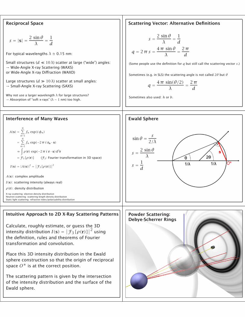
Reciprocal Space

s = |s| = 2 sinθλ

= 1d

For typical wavelengths λ � 0.15 nm:

Small structures (d� 10λ) scatter at large (“wide”) angles:→ Wide-Angle X-ray Scattering (WAXS)or Wide-Angle X-ray Diffraction (WAXD)

Large structures (d� 10λ) scatter at small angles:→ Small-Angle X-ray Scattering (SAXS)

Why not use a larger wavelength λ for large structures?→ Absorption of “soft x-rays” (λ ∼ 1 nm) too high.

Scattering Vector: Alternative Definitions

s = 2 sinθλ

= 1d

q = 2π s = 4π sinθλ

= 2πd

(Some people use the definition for q but still call the scattering vector s.)

Sometimes (e.g. in SLS) the scattering angle is not called 2θ but θ

q = 4π sin(θ/2)λ

= 2πd

Sometimes also used: h or b.

Interference of Many Waves

A(s) =N∑n=1

fn exp(iφn)

=N∑n=1

fn exp(−2π i rn · s)

⇒∫ρ(r) exp(−2π i r · s)d3r

= F3 [ρ(r)] (F3: Fourier transformation in 3D space)

I(s) = |A(s)|2 = ∣∣F3 [ρ(r)]∣∣2

A(s): complex amplitude

I(s): scattering intensity (always real)

ρ(r): density distribution

X-ray scattering: electron density distributionNeutron scattering: scattering length density distributionStatic light scattering: refractive index/polarizability distribution

Ewald Sphere

sinθ = s2/λ

s = 2 sinθλ

s = 1d

Intuitive Approach to 2D X-Ray Scattering Patterns

Calculate, roughly estimate, or guess the 3Dintensity distribution I(s) = ∣∣F3 [ρ(r)]

∣∣2 usingthe definition, rules and theorems of Fouriertransformation and convolution.

Place this 3D intensity distribution in the Ewaldsphere construction so that the origin of reciprocalspace O∗ is at the correct position.

The scattering pattern is given by the intersectionof the intensity distribution and the surface of theEwald sphere.

Powder Scattering:Debye-Scherrer Rings

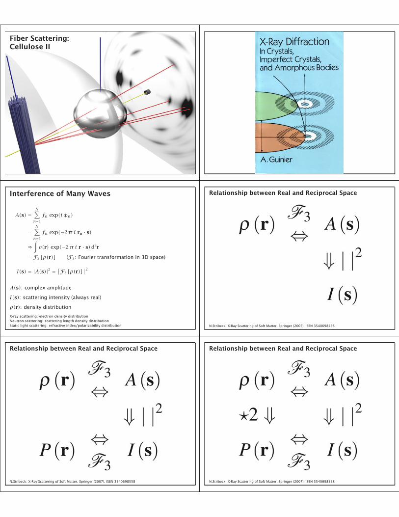
Fiber Scattering:Cellulose II

Interference of Many Waves

A(s) =N∑n=1

fn exp(iφn)

=N∑n=1

fn exp(−2π i rn · s)

⇒∫ρ(r) exp(−2π i r · s)d3r

= F3 [ρ(r)] (F3: Fourier transformation in 3D space)

I(s) = |A(s)|2 = ∣∣F3 [ρ(r)]∣∣2

A(s): complex amplitude

I(s): scattering intensity (always real)

ρ(r): density distribution

X-ray scattering: electron density distributionNeutron scattering: scattering length density distributionStatic light scattering: refractive index/polarizability distribution

Relationship between Real and Reciprocal Space

N.Stribeck: X-Ray Scattering of Soft Matter, Springer (2007), ISBN 3540698558

Relationship between Real and Reciprocal Space

N.Stribeck: X-Ray Scattering of Soft Matter, Springer (2007), ISBN 3540698558

Relationship between Real and Reciprocal Space

N.Stribeck: X-Ray Scattering of Soft Matter, Springer (2007), ISBN 3540698558

Autocorrelation Function

N.Stribeck: X-Ray Scattering of Soft Matter, Springer (2007), ISBN 3540698558

Autocorrelation Function: Patterson Function

R.-J.Roe: Methods of X-ray and Neutron Scattering in Polymer Science, Oxford University Press (2000), ISBN 0195113217

Autocorrelation Function and Disorder

dens

ityau

toco

rr.

Pair Distribution Function for Liquids (Argon)

R.-J.Roe: Methods of X-ray and Neutron Scattering in Polymer Science, Oxford University Press (2000), ISBN 0195113217

R.N.Bracewell: The Fourier Transformation and its Applications,3rd ed, McGraw-Hill (2000), ISBN 0073039381

Fourier Transformation

F(s) = F [f (x)]=∫∞−∞

f(x) exp(−2π ix s)dx

f(x) = F−1 [F(s)]

=∫∞−∞

F(s) exp(2π ix s)ds

F(s) = F3 [f (x)]

=∫f(x) exp(−2π i x · s)d3x

f(x) = F−13 [F(s)]

=∫F(s) exp(2π i x · s)d3s

Fourier Transformationin Two DimensionsR.N.Bracewell: The Fourier Transformation and its Applications,3rd ed, McGraw-Hill (2000), ISBN 0073039381

R.N.Bracewell: The Fourier Transformation and its Applications,3rd ed, McGraw-Hill (2000), ISBN 0073039381

Convolution

f(x)∗ g(x) =∫∞−∞f(u)g(x −u)du

f(x)∗ g(x) =∫∞−∞f(u)g(x− u)d3u

Shifted overlap integral of two functions.

Convolution Theorems of Fourier Transformation

f(x)∗ g(x) F⇐==⇒ F(s)G(s)

F(x)∗ g(x) F3⇐==⇒ F(s)G(s)

f (x)g(x)F⇐==⇒ F(s)∗G(s)

F(x)g(x)F3⇐==⇒ F(s)∗G(s)

Note: If you use q instead of s there will be some prefactors.The prefactors depend on the spatial dimension.

R.N.Bracewell: The Fourier Transformation and its Applications,3rd ed, McGraw-Hill (2000), ISBN 0073039381

Fourier Transformation is a Linear Operation

F [af(x)+ bg(x)]= aF [f (x)]+ bF [g(x)]

R.N.Bracewell: The Fourier Transformation and its Applications,3rd ed, McGraw-Hill (2000), ISBN 0073039381

Fourier Transformation is a Linear Operation

F [af(x)+ bg(x)]= aF [f (x)]+ bF [g(x)]

But beware:

F[af(x)+ bg(x)]2= a2F

[f(x)2

]+ b2F

[g(x)2

]

+ 2abF [f(x)g(x)]

Cross term

F [f(x)g(x)]= F [f (x)]∗ F [g(x)]

Dirac’s Delta Function (δ-Function)

Definition:

δ(x = 0) = 0∫∞−∞δ(x)dx = 1

R.N.Bracewell: The Fourier Transformation and its Applications, 3rd ed, McGraw-Hill (2000), ISBN 0073039381

δ-Function Approached by a Limit ProcessThe δ-function can be thought of as an infinitely narrow normalized distribution.

The exact shape of the distribution is not important.

∫∞−∞f(x) dx = 1 =⇒

∫∞−∞

1τf(xτ

)dx = 1 =⇒ lim

τ→0

1τf(xτ

)= δ(x)

R.N.Bracewell: The Fourier Transformation and its Applications, 3rd ed, McGraw-Hill (2000), ISBN 0073039381

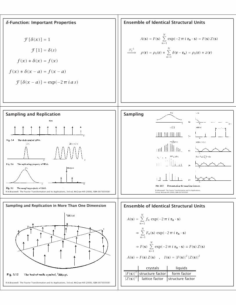
δ-Function: Important Properties

F [δ(x)] = 1

F [1] = δ(s)

f (x)∗ δ(x) = f(x)

f(x)∗ δ(x − a) = f(x − a)

F [δ(x − a)] = exp(−2π ias)

Ensemble of Identical Structural Units

A(s) = F(s)N∑n=1

exp(−2π i rn · s) = F(s)Z(s)

F−13===⇒ ρ(r) = ρ0(r)∗

N∑n=1

δ(r− rn) = ρ0(r)∗ z(r)

Sampling and Replication

R.N.Bracewell: The Fourier Transformation and its Applications, 3rd ed, McGraw-Hill (2000), ISBN 0073039381R.N.Bracewell: The Fourier Transformation and its Applications,3rd ed, McGraw-Hill (2000), ISBN 0073039381

Sampling

Sampling and Replication in More Than One Dimension

R.N.Bracewell: The Fourier Transformation and its Applications, 3rd ed, McGraw-Hill (2000), ISBN 0073039381

Ensemble of Identical Structural Units

A(s) =N∑n=1

fn exp(−2π i rn · s)

⇒N∑n=1

Fn(s) exp(−2π i rn · s)

⇒ F(s)N∑n=1

exp(−2π i rn · s) ≡ F(s)Z(s)

A(s) = F(s)Z(s) , I(s) = |F(s)|2 |Z(s)|2

crystals liquids

|F(s)|2 structure factor form factor|Z(s)|2 lattice factor structure factor

Ordered Nanostructures: Macro-lattice Morphologies

Lamellae Hex.-packed cylinders BCC spheres

Hex.-perf. layers (HPL) Ia3d Gyroid OBDD Double Diamond

Multi-block Copolymer

Block Copolymer Domain Segregation Polyelectrolyte-Surfactant Complex (PSC)

Macro-lattice Morphologies

Lamellae Hex.-packed cylinders BCC spheres

Hex.-perf. layers (HPL) Ia3d Gyroid OBDD Double Diamond

Small-Angle Scattering from Macrolattices

LAM

0 1 2 3 4 s / s*

1 : 2 : 3 : 4 : 5 : 6 : 7 . . .

PC

0 1 2 3 s / s*

1 :√

2 :√

3 : 2 :√

5 :√

6 :√

8 : 3 . . .

Ia3d

0 1 2 3 s / s*√3 : 2 :

√7 :

√8 :

√10 :

√11 :

√12 . . .

HCPC

0 1 2 3 s / s*

1 :√

3 : 2 :√

7 : 3 :√

12 :√

13 : 4 . . .

BCC

0 1 2 3 s / s*

1 :√

2 :√

3 : 2 :√

5 :√

6 :√

7 :√

8 . . .

OBDD

0 1 2 3 s / s*√2 :

√3 : 2 :

√6 :

√8 : 3 :

√10 . . .

HCPS

0 5 10 s / s*√32 : 6 :

√41 :

√68 :

√96 :

√113 . . .

FCC

0 1 2 3 s / s*√3 : 2 :

√8 :

√11 :

√12 : 4 :

√19 . . .

Pm3n

0 1 2 3 4 s / s*√2 : 2 :

√5 :

√6 :

√8 :

√10 :

√12 . . .

Dilute System (Dilute Solution or Gas)

real space scattering pattern

Particle Form Factor for Homogeneous Spheres

1e-07

1e-06

1e-05

0.0001

0.001

0.01

0.1

1

10

0 0.5 1 1.5 2 2.5R sLord Rayleigh: Proc. Roy. Soc. London A84 (1911) 25–38

Moment of Inertia (Second Moment)

1D:∫∞−∞x2 f(x)dx = −F

′′(0)4π2

In 3D this is related to the radius of gyration or Guinier radius

R.N.Bracewell: The Fourier Transformation and its Applications, 3rd ed, McGraw-Hill (2000), ISBN 0073039381

Series Expansion at Small s

I(s) = I0[

1− 43π2R2

g s2 +O(s4)

]

Guinier Approximation

I(s) = I0[

1− 43π2R2

g s2 +O(s4)

]

≈ I0 exp[−4

3π2R2

g s2]

Guinier Plot

N.Stribeck: X-Ray Scattering of Soft Matter, Springer (2007), ISBN 3540698558

Glatter Indirect Fourier-Transformation (ITP)

O.Glatter & O.Kratky (ed.), Small-Angle X-ray Scattering. Acad. Press (1982), ISBN 0122862805

Glatter Indirect Fourier-Transformation (ITP)

O.Glatter & O.Kratky (ed.), Small-Angle X-ray Scattering. Acad. Press (1982), ISBN 0122862805

Stührmann/Svergun Spherical HarmonicsMulti-pole Expansion

A(s) =N∑n=1

fn(s) exp(2π i r · s)

=∞∑�=0

�∑m=−�

a�m(s)Y�m(ψ,φ)

Dilute System

real space scattering pattern

Non-Dilute System

real space scattering pattern

Percus-Yevick Hard Sphere Structure Factor |Z(s)|2

0

0.5

1

1.5

2

2.5

0 0.5 1 1.5 2 2.5R s

η=0.1η=0.2η=0.3η=0.4η=0.5η=0.6

J.K.Percus, G.J.Yevick: Phys. Rev. 110 (1958) 1–13

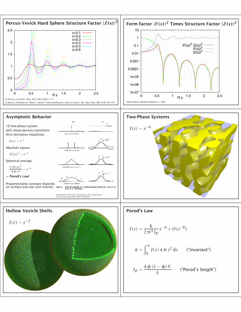
J.A.Barker, D.Henderson: What is “liquid”? Understanding the states of matter. Rev. Mod. Phys. 48 (1976) 587–671

Form factor |F(s)|2 Times Structure Factor |Z(s)|2

1e-07

1e-06

1e-05

0.0001

0.001

0.01

0.1

1

10

0 0.5 1 1.5 2 2.5R s

|F(s)|2 |Z(s)|2

|F(s)|2

|Z(s)|2

Hard sphere volume fraction η = 50%

R.N.Bracewell: The Fourier Transformation and its Applications,3rd ed, McGraw-Hill (2000), ISBN 0073039381

Asymptotic Behavior

1D two-phase systemwith sharp density transitions(first derivative impulsive):

F(s) ∼ s−1

Absolute square:

|F(s)|2 ∼ s−2

Spherical average:

2 |F(s)|24π s2

∼ s−4

→ Porod’s Law!

Proportionality constant dependson surface area per unit volume.

Two-Phase Systems

I(s) ∼ s−4

Hollow Vesicle Shells

I(s) ∼ s−2

Porod’s Law

I(s) = k2π3 lp

s−4 +O(s−6)

k =∫∞

0I(s)4π s2 ds (“invariant”)

lp = 4φ(1−φ)VS

(“Porod’s length”)

Porod’s Law

N.Stribeck: X-Ray Scattering of Soft Matter, Springer (2007), ISBN 3540698558

Deviations from Porod’s Law

N.Stribeck: X-Ray Scattering of Soft Matter, Springer (2007), ISBN 3540698558

Deviations from Porod’s Law

N.Stribeck: X-Ray Scattering of Soft Matter, Springer (2007), ISBN 3540698558

Smooth Density Transition at the Interface

R.-J.Roe: Methods of X-ray and Neutron Scattering in Polymer Science, Oxford University Press (2000), ISBN 0195113217

Fluctuation Background for Typical Polymers

R.-J.Roe: Methods of X-ray and Neutron Scattering in Polymer Science, Oxford University Press (2000), ISBN 0195113217

Chord Length Distributions

R.-J.Roe: Methods of X-ray and Neutron Scattering in Polymer Science, Oxford University Press (2000), ISBN 0195113217

Chord Length Distributions

N.Stribeck: X-Ray Scattering of Soft Matter, Springer (2007), ISBN 3540698558

Types of Lattice Disorder

1. Lattice Disorder of the First Kind

Does not destroy the coherence of the lattice.

→ Sharp peaks plus continuous background.

2. Lattice Disorder of the Second Kind

Does destroy the coherence of the lattice.

→ Broad peaks, get broader with increasing s.

Lattice Disorder of the First Kind

displacement disorder substitution disorder

Lattice Disorder, First Kind vs Second Kind

R.-J.Roe: Methods of X-ray and Neutron Scattering in Polymer Science, Oxford University Press (2000), ISBN 0195113217

Rayleigh’s Theorem / Parseval’s Theorem

F(s) = F [f (x)] =⇒∫∞−∞

∣∣f(x)∣∣2 dx =∫∞−∞|F(s)|2 ds

R.N.Bracewell: The Fourier Transformation and its Applications, 3rd ed, McGraw-Hill (2000), ISBN 0073039381

Invariant

∫|ρ(r)|2 d3r =

∫|A(s)|2 d3s =

∫I(s)d3s ≡ Q

• The invariant Q does not change if we rearrange thescatterers.

• For displacement disorder, the continuous backgroundintensity must be taken from the intensity of thesharp peaks.

• We can relate integrals in reciprocal space to integrals inreal space. This is used e.g. in the determination ofcrystallinity of semi-crystalline polymers.

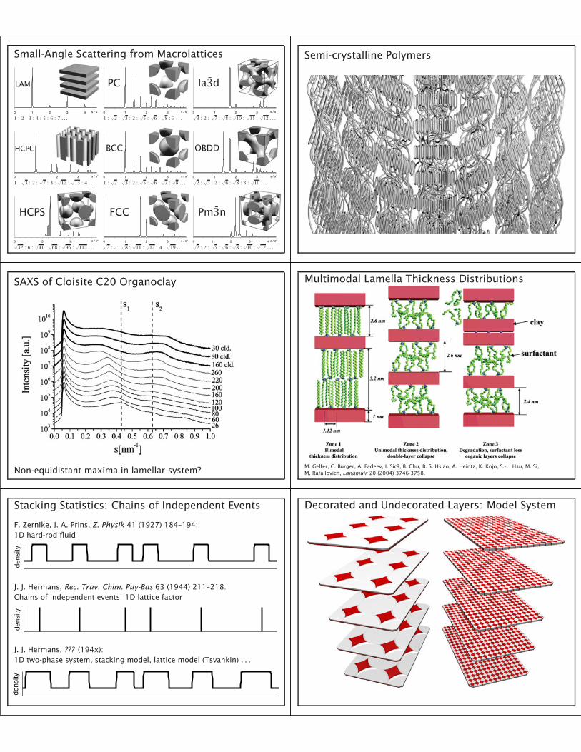
Small-Angle Scattering from Macrolattices

LAM

0 1 2 3 4 s / s*

1 : 2 : 3 : 4 : 5 : 6 : 7 . . .

PC

0 1 2 3 s / s*

1 :√

2 :√

3 : 2 :√

5 :√

6 :√

8 : 3 . . .

Ia3d

0 1 2 3 s / s*√3 : 2 :

√7 :

√8 :

√10 :

√11 :

√12 . . .

HCPC

0 1 2 3 s / s*

1 :√

3 : 2 :√

7 : 3 :√

12 :√

13 : 4 . . .

BCC

0 1 2 3 s / s*

1 :√

2 :√

3 : 2 :√

5 :√

6 :√

7 :√

8 . . .

OBDD

0 1 2 3 s / s*√2 :

√3 : 2 :

√6 :

√8 : 3 :

√10 . . .

HCPS

0 5 10 s / s*√32 : 6 :

√41 :

√68 :

√96 :

√113 . . .

FCC

0 1 2 3 s / s*√3 : 2 :

√8 :

√11 :

√12 : 4 :

√19 . . .

Pm3n

0 1 2 3 4 s / s*√2 : 2 :

√5 :

√6 :

√8 :

√10 :

√12 . . .

Semi-crystalline Polymers

SAXS of Cloisite C20 Organoclay

Non-equidistant maxima in lamellar system?

Multimodal Lamella Thickness Distributions

M. Gelfer, C. Burger, A. Fadeev, I. Sics, B. Chu, B. S. Hsiao, A. Heintz, K. Kojo, S.-L. Hsu, M. Si,M. Rafailovich, Langmuir 20 (2004) 3746-3758.

Stacking Statistics: Chains of Independent Events

F. Zernike, J. A. Prins, Z. Physik 41 (1927) 184–194:1D hard-rod fluid

dens

ity

J. J. Hermans, Rec. Trav. Chim. Pay-Bas 63 (1944) 211–218:Chains of independent events: 1D lattice factor

dens

ity

J. J. Hermans, ??? (194x):1D two-phase system, stacking model, lattice model (Tsvankin) . . .

dens

ity

Decorated and Undecorated Layers: Model System

Decorated Layers: Random Translational Stacking Disorder Undecorated Layers: Translational Stacking Disorder in Layer Normal direction only

“Turbostratic” Layers: Rotational Stacking Disorder Decorated Layers: A-B-C Stacking Sequence

Decorated Layers: A-B-A Stacking Sequence A-B-C Stacking with Twinning: First Order Markov Chains

Paracrystal? Analytical Treatment of Stacking Sequences

• Distance distributions can be multimodal.

• Distance distributions can be 3D.

• Going beyond independent events:Markov chains.

• Finite stack heights.

• Polydispersity of stack heights.

Graphite / Hexagonally Perforated Layers Multi-wall Carbon Nanotubes

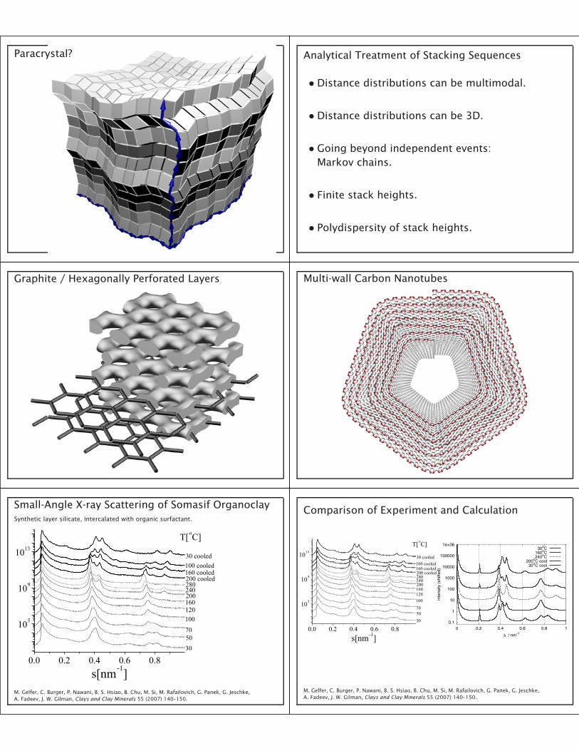
Small-Angle X-ray Scattering of Somasif OrganoclaySynthetic layer silicate, intercalated with organic surfactant.

M. Gelfer, C. Burger, P. Nawani, B. S. Hsiao, B. Chu, M. Si, M. Rafailovich, G. Panek, G. Jeschke,A. Fadeev, J. W. Gilman, Clays and Clay Minerals 55 (2007) 140–150.

Comparison of Experiment and Calculation

0.1

1

10

100

1000

10000

100000

1e+06

0 0.2 0.4 0.6 0.8 1

inte

nsity

(sh

ifted

)

s / nm-1

30oC160oC240oC

200oC cool30oC cool

M. Gelfer, C. Burger, P. Nawani, B. S. Hsiao, B. Chu, M. Si, M. Rafailovich, G. Panek, G. Jeschke,A. Fadeev, J. W. Gilman, Clays and Clay Minerals 55 (2007) 140–150.

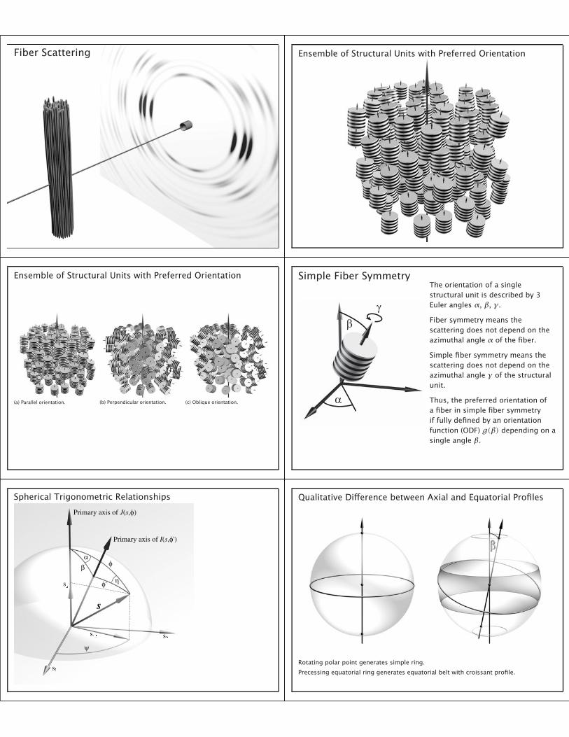
Fiber Scattering Ensemble of Structural Units with Preferred Orientation

Ensemble of Structural Units with Preferred Orientation

(a) Parallel orientation. (b) Perpendicular orientation. (c) Oblique orientation.

Simple Fiber Symmetry

β

α

γ

The orientation of a singlestructural unit is described by 3Euler angles α, β, γ.

Fiber symmetry means thescattering does not depend on theazimuthal angle α of the fiber.

Simple fiber symmetry means thescattering does not depend on theazimuthal angle γ of the structuralunit.

Thus, the preferred orientation ofa fiber in simple fiber symmetryif fully defined by an orientationfunction (ODF) g(β) depending on asingle angle β.

Spherical Trigonometric Relationships Qualitative Difference between Axial and Equatorial Profiles

Rotating polar point generates simple ring.

Precessing equatorial ring generates equatorial belt with croissant profile.

Two-point Pattern 1 Two-point Pattern 2

Four-point Pattern 1 Four-point Pattern 2

Four-point Pattern 3

Hierarchical Structures in Bone

Length scales:(a) Macroscopic bone: ∼ 1 cm(b) Osteons: ∼ 100 µm(c) Collagen fibers: ∼ 5 µm lateral, consisting of collagen fibrils: ∼ 100 nm lateral(d) Collagen molecular packing with mineral: ∼ 68 nm long period, ∼ 1.5 nm lat.(e) Single molecule triple helix: ∼ 1.0 nm lateral(f) Unmineralized collagen matrix(g) True aspect ratio.H. W. Zhou, C. Burger, I. Sics, B. S. Hsiao, B. Chu, L. Graham and M. J. Glimcher, J. Appl. Cryst. 40 (2007) S666–S668.

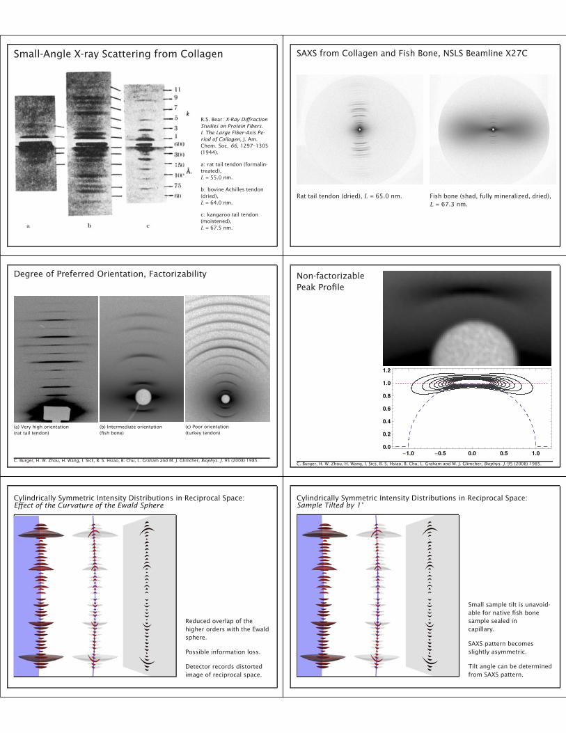
Small-Angle X-ray Scattering from Collagen

R.S. Bear: X-Ray DiffractionStudies on Protein Fibers.I. The Large Fiber-Axis Pe-riod of Collagen, J. Am.Chem. Soc. 66, 1297–1305(1944).

a: rat tail tendon (formalin-treated),L = 55.0 nm.

b: bovine Achilles tendon(dried),L = 64.0 nm.

c: kangaroo tail tendon(moistened),L = 67.5 nm.

SAXS from Collagen and Fish Bone, NSLS Beamline X27C

Rat tail tendon (dried), L = 65.0 nm. Fish bone (shad, fully mineralized, dried),L = 67.3 nm.

Degree of Preferred Orientation, Factorizability

(a) Very high orientation(rat tail tendon)

(b) Intermediate orientation(fish bone)

(c) Poor orientation(turkey tendon)

C. Burger, H. W. Zhou, H. Wang, I. Sics, B. S. Hsiao, B. Chu, L. Graham and M. J. Glimcher, Biophys. J. 95 (2008) 1985.

Non-factorizablePeak Profile

�1.0 �0.5 0.0 0.5 1.00.0

0.2

0.4

0.6

0.8

1.0

1.2

C. Burger, H. W. Zhou, H. Wang, I. Sics, B. S. Hsiao, B. Chu, L. Graham and M. J. Glimcher, Biophys. J. 95 (2008) 1985.

Cylindrically Symmetric Intensity Distributions in Reciprocal Space:Effect of the Curvature of the Ewald Sphere

Reduced overlap of thehigher orders with the Ewaldsphere.

Possible information loss.

Detector records distortedimage of reciprocal space.

Cylindrically Symmetric Intensity Distributions in Reciprocal Space:Sample Tilted by 1°

Small sample tilt is unavoid-able for native fish bonesample sealed incapillary.

SAXS pattern becomesslightly asymmetric.

Tilt angle can be determinedfrom SAXS pattern.

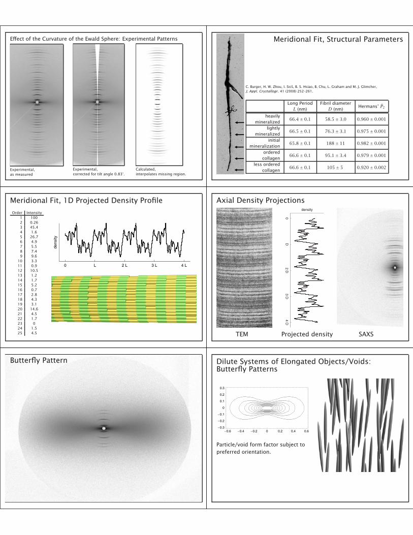
Effect of the Curvature of the Ewald Sphere: Experimental Patterns

Experimental,as measured

Experimental,corrected for tilt angle 0.83°.

Calculated,interpolates missing region.

Meridional Fit, Structural Parameters

C. Burger, H. W. Zhou, I. Sics, B. S. Hsiao, B. Chu, L. Graham and M. J. Glimcher,J. Appl. Crystallogr. 41 (2008) 252–261.

Long PeriodL (nm)

Fibril diameterD (nm)

Hermans’ P2

heavilymineralized

66.4± 0.1 58.5± 3.0 0.960± 0.001

lightlymineralized

66.5± 0.1 76.3± 3.1 0.975± 0.001

initialmineralization

65.8± 0.1 188± 11 0.982± 0.001

orderedcollagen

66.6± 0.1 95.1± 3.4 0.979± 0.001

less orderedcollagen

66.6± 0.1 105± 5 0.920± 0.002

Meridional Fit, 1D Projected Density Profile

Order Intensity1 1002 0.263 45.44 1.65 26.76 4.97 5.58 7.49 9.6

10 3.311 0.912 10.513 1.214 1.715 5.216 0.717 2.818 4.319 3.120 14.621 4.522 1.723 024 1.525 4.5

0 L 2 L 3 L 4 L

dens

ity

Axial Density Projections

0D

2 D3 D

4 D

density

TEM Projected density SAXS

Butterfly Pattern Dilute Systems of Elongated Objects/Voids:Butterfly Patterns

�0.6 �0.4 �0.2 0 0.2 0.4 0.6�0.3

�0.2

�0.1

0

0.1

0.2

0.3

Particle/void form factor subject topreferred orientation.

Butterfly Patterns for Dense Systems

�1.5 �1 �0.5 0 0.5 1 1.5

�0.6

�0.4

�0.2

0

0.2

0.4

0.6

�1.5 �1 �0.5 0 0.5 1 1.5

�0.6

�0.4

�0.2

0

0.2

0.4

0.6

�1.5 �1 �0.5 0 0.5 1 1.5

�0.6

�0.4

�0.2

0

0.2

0.4

0.6

�1.5 �1 �0.5 0 0.5 1 1.5

�0.6

�0.4

�0.2

0

0.2

0.4

0.6

�1.5 �1 �0.5 0 0.5 1 1.5

�0.6

�0.4

�0.2

0

0.2

0.4

0.6

�1.5 �1 �0.5 0 0.5 1 1.5

�0.6

�0.4

�0.2

0

0.2

0.4

0.6

2D cross-section modeled as 2D hard-disk fluid:

Structure factor modulations develop with increasing vol-ume fractions (0.05, 0.1, 0.2, 0.3, 0.4, 0.5 from left toright, top to bottom). Stacks of Platelets

Non-Dilute System of Mineral Platelets: Diskotic Arrangements

TEM (Glimcher 1991).

• Anisotropic cross-section of theplatelet-shaped min-eral crystals.

• Formation ofdiskotic stacks.

• Perturbation of thecollagen matrix.

Possible cross-section textures:

linear tangential radial spiral stack mosaic

Modified Zernike-Prins Model

Zernike-Prins 1D hard-rod fluidF. Zernike and J.A. Prins: Z. Physik 41, 184, (1927).

1D intensity distribution:

I1D(s) = 12π2 s2

Re[1−H1(s)] [1−H2(s)]

1−H1(s)H2(s)

J.J. Hermans, Rec. Trav. Chim. Pay-Bas 63, 211–218,(1944).

3D intensity distribution (perfectly oriented):

I(s12, s3) = (2π s)−1 I1D(s12) I3(s3)

Thickness distributions h and their Fourier trans-forms H:

h1(T) = (2π σ 2T )−1/2 exp

[−(T − 〈T 〉)2/(2σ 2

T )]

H1(s) = exp(2π i 〈T 〉 s − 2π2σ 2T s2)

h2(T) = Γ(ν)−1a−ν tν−1 exp(−t/a)H2(s) = (1− 2π ias)−ν

Preferred orientation:

J(s,φ) =∫ π/2

0I(s,φ′) F(φ,φ′) sinφ′ dφ′

Thickness Distributions as a Function of the Degree of Mineralization

Mineral platelet thickness distributions. Organic layer thickness distributions.

Thin mineral platelets narrowly distributed around 2.0 nm(hexagonal unit cell edge of apatite is 0.9 nm).

Larger organic layer thickness with broader distribution,no significant change with the degree of mineralization.

Complete 2D Fit of Fish Bone SAXS PatternBoth Meridional Peaks and Butterfly Pattern

Experimental. 2D Fit.