M.A.L. Nicolelis (Ed.)Progress in Brain Research, Vol. 130 2001 Elsevier Science B.V. All rights reserved

CHAPTER 3

Overcoming the limitations of correlation analysis formany simultaneously processed neural structures

Luiz A. Baccala 1,Ł and Koichi Sameshima 2

1 Telecommunications and Control Enginering Department, Escola Politecnica, Av. Prof. Luciano Gualberto, Trav. 3, #158, University ofSao Paulo, Sao Paulo, SP, CEP 05508-900, Brazil

2 Disc. Medical Informatics and Functional Neurosurgery Laboratory, School of Medicine, University of Sao Paulo, Sao Paulo, Brazil

Introduction

Despite modern methods in molecular biology, neu-roanatomy, and functional imaging, monitoring elec-tric signals from neuronal depolarization remainsimportant when evaluating the functional aspects ofboth normal and pathological neural circuitry. Cor-relation methods still rank popular and are exten-sively used to analyze the functional interaction inthe electroencephalogram (EEG), the magnetoen-cephalogram, local field potentials and more re-cently, in simultaneously recorded single- and multi-unit activity of many structures (tens to hundreds ata time). This last item has deserved increasing atten-tion due to its potential in bridging the gap betweenthe study of isolated single neurons and the under-standing of encoding and processing of informationby neuronal populations (Eichenbaum and Davis,1998; Nicolelis, 1998).

A host of other analytical techniques haveemerged, some employing information theoretic ra-tionales by assessing mutual information (Yamada et

Ł Corresponding author: Luiz A. Baccala, Telecommunica-tions and Control Enginering Department, Escola Politec-nica, Av. Prof. Luciano Gualberto, Trav. 3, #158, Univer-sity of Sao Paulo, Sao Paulo, SP, CEP 05508-900, Brazil.E-mail: baccala@lcs.poli.usp.br

al., 1993; Rieke et al., 1997; Brunel and Nadal, 1998)or interdependence between signal pairs (Schiff etal., 1996; Arnhold et al., 1999), while others areextensions of spectral analysis=coherence analysis(Glaser and Ruchkin, 1976; Duckrow and Spencer,1992; Christakos, 1997; Rosenberg et al., 1998).Despite these advances, a large fraction of neuro-scientists still chiefly rely on the cross-correlationbetween the activity of pairs of neural structures toinfer their functionality.

Like cross-correlation, all of these methods are inone way or another restricted in their calculationsto using just the signal of two structures at a time.In this article, we show that it is not only possiblebut also desirable to analyze more than two struc-tures simultaneously. Furthermore, we show alsothat effective structural inference is only possibleif simultaneous signals from many (representative)structures are jointly analyzed.

To handle many simultaneous structures, we em-ploy the recently introduced notion of partial di-rected coherence (PDC). This is a novel frequencydomain approach for simultaneous multichannel dataanalysis based on Granger causality that employsmultivariate auto-regressive (MAR) models for com-putational purposes (Baccala and Sameshima, 1999).We review PDC in Section 2 and illustrate its useful-ness via toy linear models simulating multi-electrodeEEG measurements in Section 3, where we contrast

CICERO/GALAYAA B.V./NICO3: pp. 1-15

2

it to other techniques (correlation=coherence analy-sis). We discuss an application to experimental datain Section 4. Further examples of PDC in a sin-gle- and multi-unit activity context are available inSameshima and Baccala (1999).

Partial directed coherence

The concept of partial directed coherence is the lat-est development of a number of time series anal-ysis efforts for describing how neural structuresare interconnected (Baccala and Sameshima, 1999;Sameshima and Baccala, 1999). Its remote originis the paper by Saito and Harashima (1981) whichintroduced the notion of directed coherence betweenthe activity of pairs of structures. Their method al-lows factoring the classical coherence function (thefrequency domain counterpart of correlation analy-sis) of a pair of structures into two ‘directed co-herences’: one representing the feedforward and theother one representing the feedback aspects of theinteraction between these two neural structures. Ex-amples of use of pairwise directed coherence instudying the relation between Parkinson’s tremorand lack of feedback in motor control are containedin Schnider et al. (1989).

In an attempt to generalize directed coherenceto a context of analysis of more than two simulta-neously processed structures, the so-called methodof directed transfer function (DTF) was introducedwith several equivalent variants (Franaszczuk et al.,1994; Baccala and Sameshima, 1998; Baccala et al.,1998). This method was applied to foci determina-tion and to EEG studies in mesial temporal lobeseizure (Franaszczuk et al., 1994). Details on DTFare contained in Appendix A.

In their original paper, Saito and Harashima(1981) allude to a possible rationale for their method.This concept is now known as Granger causal-ity (Granger, 1969). According to it, an observedtime series x.n/ Granger-causes another series y.n/,if knowledge of x.n/’s past significantly improvesprediction of y.n/; this kind of predictability im-provement is not reciprocal, i.e. x.n/ may Granger-cause y.n/ without y.n/ necessarily Granger-caus-ing x.n/. This lack of reciprocity is the basic prop-erty behind the determination of the direction ofinformation flow between pairs of structures which,

in turn, is the basis for decomposing classical coher-ence into directed feedforward and feedback coher-ence factors.

Following that rationale, we investigated howgeneralizations, like DTF, of directed coherence toN simultaneously processed structures compared tostatistical tests of Granger causality for N simulta-neous time series (Baccala et al., 1998). We real-ized that DTF provided a physiologically interestingfrequency domain picture, yet structural inferencebased on its computation did not always agree withthe result of Granger causality tests (GCT). We couldshow that this was due to intrinsic aspects of DTF’sdefinition (Baccala and Sameshima, 1999) (see alsoAppendix A).

Because Granger causality is a more fundamentalconcept than the ad hoc generalization representedby DTF, we went on to introduce the notion of partialdirected coherence (Baccala and Sameshima, 1999).This new structural connectivity estimator relies onthe simultaneous processing of N ½ 2 time seriesand is able to expose a frequency domain picture ofthe feedforward and feedback interactions betweeneach and every pair of structures within the set ofN simultaneously processed signals. Perhaps moreimportantly, PDC reflects Granger causality closelyby paralleling the definition of Granger causality testestimators.

The main preliminary ingredient of both PDC andGCT (and of DTF as well, but in a fundamentallydifferent way) is their practical use of multivariateautoregressive models as exemplified for N D 3simultaneously monitored structures in the model

24

x1.n/

x2.n/

x3.n/

35 D

pXrD1

24

a11.r/ a12.r/ a13.r/

a21.r/ a22.r/ a23.r/

a31.r/ a32.r/ a33.r/

35

ð24

x1.n � r/

x2.n � r/

x3.n � r/

35 C

24

w1.n/

2.n/

w3.n/

35

(1)

In this model, x1.n/ depends on its own pastvalues x1.n�r/ through the coefficients a11.r/ while,for example, x1.n/’s dependence on the past valuesof the other series like x2.n �r/ is through the a12.r/

coefficients. As such, the time series x2.n/ onlyGranger-causes x1.n/ if we can statistically showthat a12.r/ 6D 0 for some values of r . Or equivalently,

CICERO/GALAYAA B.V./NICO3: pp. 1-15

3

rejecting the null hypothesis of ai j.r/ D 0 meansthat x j .n/ does Granger-cause xi.n/.

The partial directed coherence from series j toseries i , at frequency f can be defined as

³i j. f / D Nai j. f /pa j . f /H a j . f /

(2)

where

Nai j . f / D

8>><>>:

1 �pP

rD1ai j .r/e� j2³ f r ; if i D j

�pP

rD1ai j .r/e� j2³ f r ; otherwise (3)

and a j . f / is the vector

a j . f / D

264

Na1 j . f /:::

NaN j . f /

375 (4)

Because of its dependence on ai j .r/ in Eq. 3,the nullity of ³i j. f / at a given frequency implieslack of Granger causality from x j .n/ to xi .n/ atthat frequency. PDC is, therefore, a direct frequencydomain counterpart of GCT.

Though further details on PDC are contained else-where (Baccala and Sameshima, 1999), a compactsummary is available at Appendix A together withits relation to DTF. Methods of MAR model fit-ting are reviewed elsewhere (Marple, 1987). In thenext section, we discuss some examples of PDC’sapplication contrasting it to other techniques.

Illustrative simulations

To provide objective comparisons of PDC with othertechniques, we use time series generated from knownlinear toy models. In this case, exact theoreticalcalculations of pairwise cross-correlation, classicalcoherence, DTF and PDC can be made and allowexposing all the relative methodological merits ofeach approach while avoiding possible pitfalls ofexperimental signals collected from neural systemswith unknown structure. The use of toy models isfurther motivated by the desire to investigate pos-sible structural inference impairments when simul-taneously processing fewer than the N structuresimportant to the dynamics.

The first toy model example, mimicking localfield potential measurements along hippocampal

structures, is represented by the following set oflinear difference equations with N D 7 structures:

Model I

x1.n/ D 0:95p

2x1.n � 1/ � 0:9025x1.n � 2/

C w1.n/

x2.n/ D �0:5x1.n � 1/ C w2.n/

x3.n/ D 0:4x2.n � 2/ C w3.n/

x4.n/ D �0:5x3.n � 1/ C 0:25p

2x4.n � 1/

C 0:25p

2x5.n � 1/ C w4.n/

x5.n/ D �0:25p

2x4.n � 1/

C 0:25p

2x5.n � 1/ C w5.n/

x6.n/ D 0:95p

2x6.n � 1/ � 0:9025x6.n � 2/

C w6.n/

x7.n/ D �0:1x6.n � 2/ C w7.n/

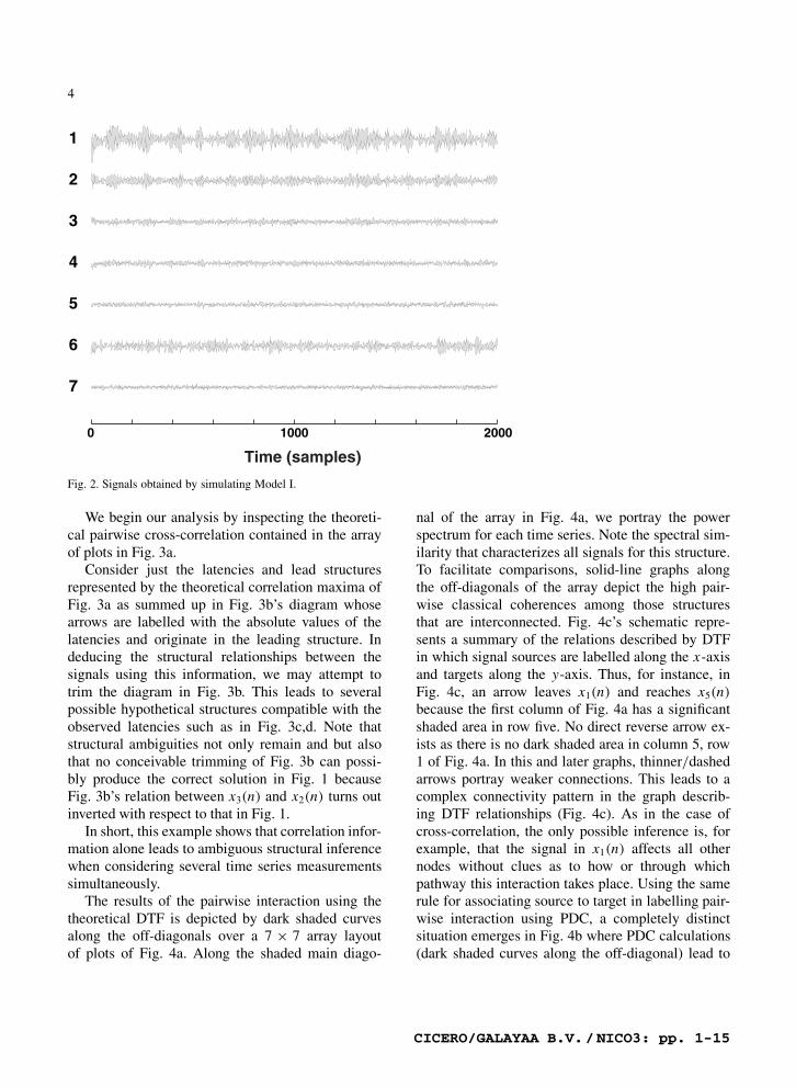
with wi .n/ standing for innovation noises.These equations are designed so that x1.n/ be-

haves as an oscillator driving the other structures,either directly or indirectly, according to the dia-gram in Fig. 1. Note that the interaction betweenx1.n/ and x3.n/ is both via a direct path and viaan indirect route through x2.n/. The dynamics ofthe pair x4.n/ and x5.n/ is designed so that theyjointly represent an oscillator, whose intrinsic char-acteristics are due to their mutual signal feedback butwhich are entrained to the rest of the structure viax3.n/. The signals x6.n/ and x7.n/ belong to a to-tally separate substructure where x6.n/ is designed togenerate oscillations at the same frequency as x1.n/;x7.n/ does not feedback anywhere. A sample of thesignals produced in this way can be appreciated inFig. 2.

31

2

4 5

6 7

Fig. 1. Signal flow diagram for Model I.

CICERO/GALAYAA B.V./NICO3: pp. 1-15

4

1

2

3

4

5

6

7

0 1000 2000

Time (samples)

Fig. 2. Signals obtained by simulating Model I.

We begin our analysis by inspecting the theoreti-cal pairwise cross-correlation contained in the arrayof plots in Fig. 3a.

Consider just the latencies and lead structuresrepresented by the theoretical correlation maxima ofFig. 3a as summed up in Fig. 3b’s diagram whosearrows are labelled with the absolute values of thelatencies and originate in the leading structure. Indeducing the structural relationships between thesignals using this information, we may attempt totrim the diagram in Fig. 3b. This leads to severalpossible hypothetical structures compatible with theobserved latencies such as in Fig. 3c,d. Note thatstructural ambiguities not only remain and but alsothat no conceivable trimming of Fig. 3b can possi-bly produce the correct solution in Fig. 1 becauseFig. 3b’s relation between x3.n/ and x2.n/ turns outinverted with respect to that in Fig. 1.

In short, this example shows that correlation infor-mation alone leads to ambiguous structural inferencewhen considering several time series measurementssimultaneously.

The results of the pairwise interaction using thetheoretical DTF is depicted by dark shaded curvesalong the off-diagonals over a 7 ð 7 array layoutof plots of Fig. 4a. Along the shaded main diago-

nal of the array in Fig. 4a, we portray the powerspectrum for each time series. Note the spectral sim-ilarity that characterizes all signals for this structure.To facilitate comparisons, solid-line graphs alongthe off-diagonals of the array depict the high pair-wise classical coherences among those structuresthat are interconnected. Fig. 4c’s schematic repre-sents a summary of the relations described by DTFin which signal sources are labelled along the x-axisand targets along the y-axis. Thus, for instance, inFig. 4c, an arrow leaves x1.n/ and reaches x5.n/

because the first column of Fig. 4a has a significantshaded area in row five. No direct reverse arrow ex-ists as there is no dark shaded area in column 5, row1 of Fig. 4a. In this and later graphs, thinner=dashedarrows portray weaker connections. This leads to acomplex connectivity pattern in the graph describ-ing DTF relationships (Fig. 4c). As in the case ofcross-correlation, the only possible inference is, forexample, that the signal in x1.n/ affects all othernodes without clues as to how or through whichpathway this interaction takes place. Using the samerule for associating source to target in labelling pair-wise interaction using PDC, a completely distinctsituation emerges in Fig. 4b where PDC calculations(dark shaded curves along the off-diagonal) lead to

CICERO/GALAYAA B.V./NICO3: pp. 1-15

5

1

2

3

4

5

6

-50 0 50

1

7

2 3 4 5 6 7

(a)

1

3

2

4

5

2

257

5 7

4

11

2

(b)

(c)

1 3

2

4 5

2

5

7

2

114

5

(d)

1 3

2

4 5

2

5

7

2

114

Fig. 3. The theoretical autocorrelations are shown along the main diagonal and, below it, all the theoretical cross-correlation functions areplotted (a), with the x-axis scale ranging from �50 to 50 sample points, and the y-axis is between �1 and 1. Directed graph summarizingsignal propagation latency information (encoded via arrow labels) contained in the cross-correlation function (b). Two possible simplifiedstructures compatible with the theoretically calculated latencies are shown in (c) and (d). Note that, the graph simplification from (c) to(d), the connection 1 ! 4 (with propagation latency 5 time units) is removed because it can be explained by the pathway 1 ! 3 ! 4with the same total propagation latency value.

the correct structure of Fig. 4d (compare with Fig. 1).We next slightly increase the complexity of this

example by adding a feedback from x5.n/ to x1.n/.This is accomplished by rewriting the first equationin Model I as

x1.n/ D 0:95p

2x1.n � 1/ � 0:9025x1.n � 2/

C 0:5x5.n � 2/ C w1.n/ (5)

in accord with the diagram of Fig. 5.As in the previous case, the theoretical DTF is

difficult to analyze (Fig. 6a,c), as opposed to PDC(Fig. 6b,d) which clearly reflects the newly addedfeedback. This pattern of straightforward analysisusing PDC carries over to a practical simulationscenario of using 500 data points where the feed-back-free situation (Fig. 7a) is easily distinguishablefrom that when feedback from x5.n/ to x1.n/ ispresent (Fig. 7b).

To provide some sense of the potential temporalresolution of the method, we display the time evo-

lution of PDCs involving x1.n/ and x5.n/ (Fig. 8)while randomly switching the feedback on and off.Each PDC estimate comprises the use of 250 simu-lated data points with 50% overlap between adjacentdata segments.

In comparing these examples, note that DTF’sgraph has arrows connecting almost all structureswhen the feedback is switched on (Fig. 6c); thisis related to the fact that the PDC graph containspathways (direct or indirect) that connect any twostructures. Some arrows in Fig. 6c are missing(x2.n/ ! x1.n/, x3.n/ ! x1.n/, x3.n/ ! x5.n/).Their presence would have made Fig. 6c’s graphfully connected. Though corresponding to existingsignal pathways, the missing arrows correspond tosmall (but theoretically nonzero) DTFs that reflectthe weakness of the connection strength of the to-tal pathways between structures that are far apartfrom one another. In fact, DTF can be interpretedas a marker for signal energy ‘reachability’ (see

CICERO/GALAYAA B.V./NICO3: pp. 1-15

6

DTF PDC

1

2

3

4

5

6

7

1 2 3 4 5 76

1

2

3

4

5

6

7

1 2 3 4 5 76

(a) (b)

(c) (d)

1 3

2

4 5

6 7

1 3

2

4 5

6 7

Fig. 4. Comparison between the theoretical DTF (a) (and its inferred structural interactions (c)) and the theoretical PDC results (b) (withits signal flow diagram (d)). In both cases the signal flow graphs are constructed by assigning an arrow from the source structure (x-axis)to the targets (y-axis) when dark shaded areas are significant. The spectral densities for the time series are depicted along the shadedmain diagonal of the arrays. The pairwise classical coherences (solid lines) are also depicted. In all plots, the x-axis represents thenormalized frequency in the 0 to 0.5 range, while the y-axis for power spectrum plots is scaled between 0 and peak value and values forthe other coherence plots lie between 0 and 1.

Remark 3 in Appendix A) and must be analyzedwith care. For example, examine the dip in the DTFfrom x2.n/ to x3.n/ in Figs. 4a and 6a. It coincideswith the maximum of the power spectrum of boththese series. Rather than mean lack of pathway con-nection at that frequency, this dip exemplifies (by

1 3

2

4 5

6 7

Fig. 5. Schematic diagram describing the inclusion of feedbackfrom x5.n/ to x1.n/ into Model I.

model design) how the energy reaching a struc-ture (x3.n/) from another structure (x1.n/) at onefrequency may be almost exactly cancelled by theenergy coming through another pathway (x2.n/) dueto a phase inversion in the signal.

To emulate scalp EEG, our second example em-ployed

Model II

x1.n/ D 1:8982x1.n � 1/ � 0:9025x1.n � 2/

C w1.n/

x2.n/ D 0:9x1.n � 2/ C w2.n/

x3.n/ D 0:85x2.n � 2/ C w3.n/

x4.n/ D 0:82x1.n � 2/ C 0:6x6.n � 3/ C w4.n/

x5.n/ D �0:9x6.n � 2/ C 0:4x2.n � 4/ C w5.n/

x6.n/ D 0:9x5.n � 2/ C w6.n/

CICERO/GALAYAA B.V./NICO3: pp. 1-15

7

1 3

2

4 5

6 7

1 4

6 7

1

2

3

4

5

6

7

1 2 3 4 5 76

1

2

3

4

5

6

7

1 2 3 4 5 76

(a) (b)

(c) (d)

DTF PDC

53

2

Fig. 6. Comparison between the theoretical DTF (a) (and its inferred structural interactions (c)) and the theoretical PDC results (b) (withits signal flow diagram (d)) after turning on the feedback from x5.n/ to x1.n/. Spectral densities for the time series are depicted along theshaded main diagonal of the arrays. The pairwise classical coherences (solid lines) are also depicted. Thin=dashed arrows portray weakerconnections.

PDC without feedback PDC with feedback

1

2

3

4

5

6

7

1 2 3 4 5 76

1

2

3

4

5

6

7

1 2 3 4 5 76

(a) (b)

Fig. 7. Estimated PDC for Model I without (a) and with (b) feedback from x5.n/ to x1.n/ using 500 simulated points. Note how x6.n/

and x7.n/ show residual classical coherence with the other time series, despite their lack of direct connection.

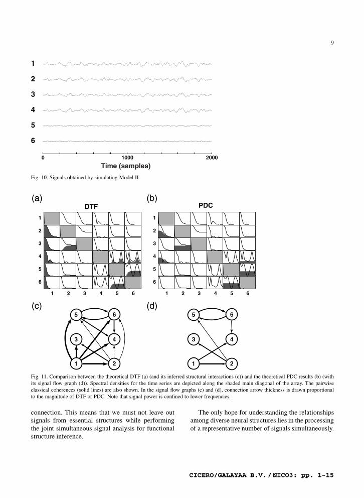
where x1.n/ is an oscillator driving, directly or indi-rectly, all the other structures. In this emulation, theodd numbered signals represent the left hemisphere

leaving the other ones to map the other hemisphereas in Fig. 9. An example of the simulated signals isportrayed in Fig. 10.

CICERO/GALAYAA B.V./NICO3: pp. 1-15

8

0

.5

1

ONOFF

Feedback Connection 1 ← 5

PDC 1 ← 5

Classical Coherence

Time (samples) 0 2000 4000 6000 8000 10000 12000

PDC 5 ← 1

Fre

q.

0

.5

Fre

q.

0

.5

Fre

q.

0

.5

(a)

(b)

(c)

(d)

Fig. 8. Gray scale plots show the time evolution of the PDC (b and c) and classical coherence (d) between structures 1 and 5 calculatedfrom 250 simulated data point segments (overlapping by 50%) as the feedback from x5.n/ and x1.n/ in Model I is switched on and off(a). The evolution of the classical coherence between these structures is also shown (d).

DTF results are shown in Fig. 11a togetherwith its corresponding inferred signal flow graphin Fig. 11c. Note that DTF correctly identifies x1.n/

as the source driving all other structures (this is thebasis of DTF’s success as an identifier of epilepticfoci in Franaszczuk et al. (1994)). As in the previousexample, however, DTF remains ambiguous as to thepathway actually followed by the signal. These possi-ble signal pathway alternatives turn out resolved in amuch simpler fashion by examining PDC in Fig. 11bwhich leads to a correct signal flow graph (Fig. 11d).

1 2

3 4

5 6

Fig. 9. Signal flow diagram for Model II.

Matching PDC calculations using simulated ratherthan theoretical values are shown in Fig. 12. Accord-ing to PDC, x1.n/’s role as a signal source for thewhole structure is equally well deducible.

A question that can arise about the use of PDCregards what happens when calculations are basedon the processing of a reduced number of structuresthan are actually representative of the structure anddynamics of the process. Suppose we want to inferthe direct interhemispheric influence by looking onlyat pairs of signals from both hemispheres alongthe sagittal plane, i.e. by computing the pairwisePDC of the pairs like (x1.n/; x2.n/), (x3.n/; x4.n/)and (x5.n/; x6.n/) without making joint calculationsinvolving the other structures.

The results of these separate pairwise analyses areshown in Fig. 13c, 13b and 13a, respectively. In thepresence of actual connections as for Fig. 13a,c, theirmutual feedback is correctly deduced from simulateddata, as opposed to the relationship between x3.n/

and x4.n/, where feedback presence is incorrectlydetected despite the absence of an actual direct inter-

CICERO/GALAYAA B.V./NICO3: pp. 1-15

9

1

2

3

4

5

6

0 1000 2000

Time (samples)

Fig. 10. Signals obtained by simulating Model II.

DTF PDC

1

2

3

4

5

6

1 2 3 4 65

1

2

3

4

5

6

1 2 3 4 65

1 2

3 4

5 6

3 4

5 6

21

(a) (b)

(c) (d)

Fig. 11. Comparison between the theoretical DTF (a) (and its inferred structural interactions (c)) and the theoretical PDC results (b) (withits signal flow graph (d)). Spectral densities for the time series are depicted along the shaded main diagonal of the array. The pairwiseclassical coherences (solid lines) are also shown. In the signal flow graphs (c) and (d), connection arrow thickness is drawn proportionalto the magnitude of DTF or PDC. Note that signal power is confined to lower frequencies.

connection. This means that we must not leave outsignals from essential structures while performingthe joint simultaneous signal analysis for functionalstructure inference.

The only hope for understanding the relationshipsamong diverse neural structures lies in the processingof a representative number of signals simultaneously.

CICERO/GALAYAA B.V./NICO3: pp. 1-15

10

PDC

1

2

3

4

5

6

1 2 3 4 65

Fig. 12. Estimated PDC for Model II using 500 simulated datapoints.

An application to experimental data

We illustrate PDC in connection to local field poten-tials recorded from a rat in exploratory behavior.The simultaneously processed structures comprisethe hippocampal CA1 field, somatosensory (A3) andmotor (A10) cortical areas and the dorsal raphe(DR), where rhythmic oscillations in the theta rangeare observed during desynchronized sleep and alertstates. Detailed DTF analysis of the same record of

1 2

3 4

5 6

65

3 4

1

2

2

1

3

4

4

3

5

6

6

5

1 2

(a)

(b)

(c)

PDC

Fig. 13. PDC results of processing pairwise structures (5,6) (a), (3,4) (b), and (1,2) (a) representing opposite hemispheres in Model IIthat show the possibility of incorrect structural inference for the pair (3,4) (b) when not all the structures relevant to the dynamics of themodel are considered jointly.

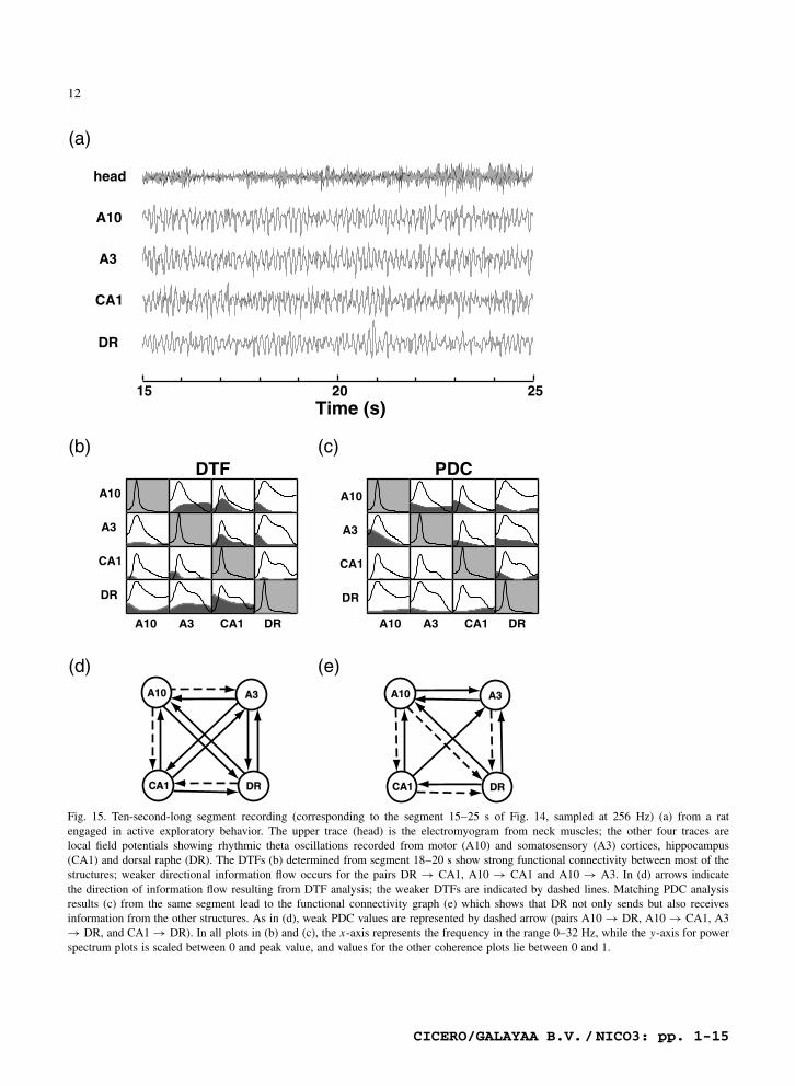
these four jointly processed structures appeared inBaccala et al. (1998) with special attention to therelationship between CA1 and A3. Fig. 14 depictsthe PDC time evolution between these structures us-ing the electromyogram from neck muscles to labelbehavioral states. For the first 30 s of this recordingsegment, the rat actively explored a lighted cage,then gradually turned inactive as can be followedby electromyogram. Around 52 s, the rat resumedthe exploratory behavior when the cage lights wereturned off. As attested by looking at classical co-herence and recording traces of Figs. 15 and 16,rhythmic oscillations are more prominent during ac-tive exploratory behavior.

In choosing special episodes in this record weconsider the period lasting between 18 and 20 s(Fig. 15a) as characterized by high-amplitude elec-tromyographic activity of neck muscles. The mainfeature of the DTF’s interactions (Fig. 15b) results inthe fully connected graph (Fig. 15d) that portrays theactive participation of all structures. PDC (Fig. 15c)reveals the underlying signal feedback pattern (two-way interactions) and highlights DR’s possibly im-portant role. A drastically different picture emergesfor the segment between 48 and 50 s of this samerecord (Fig. 16a) when the animal’s neck musclesshow low activity. DTF interactions (Fig. 16b) pro-

CICERO/GALAYAA B.V./NICO3: pp. 1-15

11

PDC A3 ← CA1

Hz

0 10 20 30 40 50

Classical Coherence

Hz

Time (s) 0 10 20 30 40 50 60

0 10 20 30 40 50

PDC CA1← A3

Hz

0 10 20 30 40 50

0

.5

1

head

EMG

Fig. 14. Time evolution of the PDC analysis highlighting the relationship between A3 and CA1 for a rat whose exploratory behavior islabelled via the electromyogram (EMG) from its neck muscles. A gray scale is used to represent the magnitude of PDC and classicalcoherence. The corresponding time evolution of the DTF between these structures appeared in Baccala et al. (1998).

duce a more sparsely connected graph (Fig. 16d) ascharacterized by fewer strong connections. In com-paring PDC calculations Fig. 15c,e against Fig. 16c,eone notices DR’s role of reversal switching from be-ing predominantly a source to being an informationsink. Furthermore, note how the influence of CA1over DR is essentially indirect with the signal firstflowing through A3 and A10 in Fig. 16e, in sharpcontrast to the PDC functional connectivity graphcorresponding to the exploratory behavior segment(Fig. 15e), where all structures receive substantialinfluence from dorsal raphe (DR). Also in the quietstate (Fig. 16e), information is mostly being re-layed from the other structures through A10 to DR.This example highlights the distinct and potentiallyinteresting functional connectivity patterns that char-acterize different behavioral states.

Conclusions and comments

By analyzing linear toy models, we show PDC’s su-perior performance over other commonly used meth-ods specially cross-correlation and classical coher-ence, while DTF analysis provides complementary

information whose analysis is less clear than PDC’s.The main advantage of PDC lies in the graphi-cally unambiguous frequency domain display of therelationships among simultaneous measurements ofseveral time series as PDC can clearly expose thefeedback structure between directly connected pairsof neural elements provided all the structures repre-sentative of the dynamics are jointly processed.

Simultaneous recordings as well as the analysisof representative samples of neural elements throughmulti-site multichannel recording is therefore crucialfor deducing functional connectivity. This acquiresspecial importance in view of the fact that evenPDC pairwise analysis may induce misleading con-clusions about the nature of the interaction amongneural elements. We therefore conclude that the useof techniques based on the processing pairwise timeseries are doomed to failure and that only the pro-cessing of many simultaneous structures can leadto an understanding of neural ensemble informationprocessing and coding.

Though unaddressed in this paper, statistical is-sues are important. While asymptotic results for theai j .r/ coefficients exist and lead to Granger causality

CICERO/GALAYAA B.V./NICO3: pp. 1-15

12

A10

A3

CA1

DR

A10 A3 DRCA1

DTFA10

A3

CA1

DR

A10 A3 DRCA1

PDC

head

A10

A3

CA1

DR

15 20 25Time (s)

A3

CA1 DR

(a)

(b) (c)

(d) (e)A10 A3

CA1 DR

A10

Fig. 15. Ten-second-long segment recording (corresponding to the segment 15–25 s of Fig. 14, sampled at 256 Hz) (a) from a ratengaged in active exploratory behavior. The upper trace (head) is the electromyogram from neck muscles; the other four traces arelocal field potentials showing rhythmic theta oscillations recorded from motor (A10) and somatosensory (A3) cortices, hippocampus(CA1) and dorsal raphe (DR). The DTFs (b) determined from segment 18–20 s show strong functional connectivity between most of thestructures; weaker directional information flow occurs for the pairs DR ! CA1, A10 ! CA1 and A10 ! A3. In (d) arrows indicatethe direction of information flow resulting from DTF analysis; the weaker DTFs are indicated by dashed lines. Matching PDC analysisresults (c) from the same segment lead to the functional connectivity graph (e) which shows that DR not only sends but also receivesinformation from the other structures. As in (d), weak PDC values are represented by dashed arrow (pairs A10 ! DR, A10 ! CA1, A3! DR, and CA1 ! DR). In all plots in (b) and (c), the x-axis represents the frequency in the range 0–32 Hz, while the y-axis for powerspectrum plots is scaled between 0 and peak value, and values for the other coherence plots lie between 0 and 1.

CICERO/GALAYAA B.V./NICO3: pp. 1-15

13

A10

A3

CA1

DR

A10 A3 DRCA1

DTFA10

A3

CA1

DR

A10 A3 DRCA1

PDC

head

A10

A3

DR

45 50 55

CA1

Time (s)

(a)

(b) (c)

(d) (e)

A3

CA1

A10 A3

CA1 DR DR

A10

Fig. 16. Ten-second-long recording segment (a) (corresponding to the 45–55 s behavioral segment of Fig. 14, sampled at 256 Hz)showing the transition from the quiet state to active exploratory behavior induced by turning lights off at around 52 s. See Fig. 15for details on channel labels. Note that theta waves become prominent in all four brain structures concomitantly with the onset ofelectromyographic activity. When compared to Fig. 15d, DTFs determined from segment 48–50 s (b) shows a larger number of weakerfunctional connections (d) indicated by dashed arrows. The corresponding PDC analysis (c) and its functional connectivity graph (e)portray weaker connectivity from DR to all other structures. During this episode the DTF graph connectivities (d), CA1 ! DR and A3! DR are not matched by direct connections in the PDC graph (e). They can, however, be explained respectively by the existence ofindirect signal pathways CA1 ! A10 ! DR and A3 ! A10 ! DR. Note also that DR is essentially an information sink while CA1 ismainly an information source. In all plots in (b) and (c), the x-axis represents the frequency in the 0 to 32 Hz range, while the y-axis forpower spectrum plots is scaled between 0 and peak value, and for coherence plots between 0 and 1.

CICERO/GALAYAA B.V./NICO3: pp. 1-15

14

tests (Lutkepohl, 1993; Baccala et al., 1998), theirusefulness is less clear because of the ‘quasi-sta-tionary’ nature of neural signals. More importantlyperhaps, as our examples show, is the fact that weakconnections can be barely detectable. This is spe-cially true in the case of DTF where the effect ofweakly connected signal pathways is compounded(for example see Fig. 6a,c). Also, the number of si-multaneously processed structures affects the achiev-able temporal resolution as more data points becomenecessary to insure statistically reliable detection ofweak connections.

Finally, it is important to have in mind that,though based on linear time series modelling, PDCproves applicable and useful for the analysis of mul-tiple structures that involve some levels of nonlinearinteractions as discussed in Sameshima and Baccala(1999). In fact, to our knowledge, PDC is the onlyexisting practical method that effectively goes be-yond pairwise analysis and is capable of efficientlyhandling multiple structures simultaneously as is es-sential for reliable functional structural inference.

Acknowledgements

This work received financial support from CNPq,PRONEX and FAPESP grants to the authors.

Appendix A

If xi .n/, 1 � i � N , represent simultaneously processed discretetime signals, the canonical way to represent the relationshipbetween these time series in the frequency domain is via theirjoint power spectral density matrix, which reads

S. f / D24

S1. f / S12. f / S13. f /

S21. f / S2. f / S23. f /

S31. f / S32. f / S3. f /

35 (6)

in a N D 3 example. In general, one may calculate S. f / byusing a multivariate (vector) autoregressive model (Priestley,1981; Lutkepohl, 1993)

264

x1.n/

:::

xN .n/

375 D

pXrD1

Ar

264

x1.n � r/

:::

xN .n � r/

375 C

264

w1.n/

:::

wN .n/

375

(7)

with wi .n/ standing for white uncorrelated innovation noises.The coefficient matrices Ar , for each lag r, may be estimatedeither using least squares or fast maximum entropy methods. Theappropriate order of the model p can be inferred using Akaike’sAIC criterion (Marple, 1987). In this case, the power spectral

density matrix may be written as

S. f / D H. f /Σ H H . f / (8)

where

Σ D

264

¦ 211 : : : ¦1N

:::

: : ::::

¦N1 : : : ¦ 2N N

375 (9)

is the covariance matrix of wi .n/, and

H. f / D A�1

. f / D .I � A. f //�1 (10)

with

A. f / DpX

rD1

Ar z�r

þþþþþzDe� j 2³ f

At this point, one option for describing the mutual interactionbetween pairs of time series may be obtained through a general-ized definition of the directed coherence from j to i as (Baccalaand Sameshima, 1998; Baccala and Sameshima, 1999)

i j . f / D ¦ j j Hi j . f /pSi . f /

; (11)

where

Si . f / DNX

jD1

¦ 2j j

þþHij . f /þþ2

: (12)

Remark 1 The definition of DTF in Franaszczuk et al. (1994)is a special case where ¦ii are made equal to 1 in Eq. 11.Because of its relationship to the power spectral density ma-trix,

þþi j . f /þþ may be interpreted as a fraction of the power

originating in x j .n/ that reaches xi .n/.An alternative way to describe the mutual interaction is

via the ai j .r/ elements of Ar , i.e. by testing Granger causal-ity directly. If Nai j . f / be A. f /’s i; j -th element, i.e. the i-thcomponent of the j -th column a j . f / of A. f /. After suitablenormalization, discussed elsewhere (Baccala and Sameshima,1999), one possible definition for partial directed coherence is

³i j . f / D Nai j . f /pa j . f /H a j . f /

(13)

Remark 2 This name, ‘partial directed coherence’, comesfrom an interpretation of ³i j . f / as factor in the partial coher-ence i j . f / between two time series (Bendat and Piersol, 1986;Baccala and Sameshima, 1999).

Remark 3 The relationship between PDC and DTF is thatthey are based, respectively, on the matrices A. f / and H. f /

which are inverses of one another. This inverse matrix relation-ship occurs in graph theory where a matrix like A. f / describesthe connections of directed graphs while a matrix like H. f / isanalogous to the graph reachability matrix which records thegraph structures reachable from a given node (Baccala et al.,1991).

Remark 4 When N D 2, PDC leads exactly to the sameestimator as DTF (Baccala and Sameshima, 1999).

CICERO/GALAYAA B.V./NICO3: pp. 1-15

15

References

Arnhold, J., Grassberger, P., Lehnertz, K. and Elger, C.E. (1999)A robust method for detecting interdependencies: applicationto intracranially recorded EEG. Physica D, 134: 419–430.

Baccala, L.A. and Sameshima, K. (1998) Directed Coherence: Atool for exploring functional interactions among brain struc-tures. In: M.A.L. Nicolelis (Ed.), Methods for Neural Ensem-ble Recordings. CRC Press, Boca Raton, FL, pp. 179–192.

Baccala, L.A. and Sameshima, K. (2001) Partial directed co-herence a new concept in neural structure determination.Biol. Cybern., 84: 463-474.

Baccala, L., Nicolelis, M., Yu, C. and Oshiro, M. (1991) Struc-tural analysis of neural circuits using the theory of directedgraphs. Comp. Biomed. Res., 24: 7–28.

Baccala, L.A., Sameshima, K., Ballester, G., Valle, A.C. andTimo-Iaria, C. (1998) Studying the interaction between brainstructures via directed coherence and Granger causality. Appl.Sig. Process., 5: 40–48.

Bendat, J.S. and Piersol, A.G. (1986) Random Data: Analysisand Measurement Procedures. John Wiley, New York, 2nd ed.

Brunel, N. and Nadal, J.P. (1998) Mutual information, Fisher in-formation, and population coding. Neural Comput., 10: 1731–1757.

Christakos, C.N. (1997) On the detection and measurement ofsynchrony in neural populations by coherence analysis. J.Neurophysiol., 78: 3453–3459.

Duckrow, R.B. and Spencer, S.S. (1992) Regional coherence andthe transfer of ictal activity during seizure onset in the medialtemporal lobe. Electroencephalogr. Clin. Neurophysiol., 82:415–422.

Eichenbaum, H.B. and Davis, J.L. (Eds.) (1998) Neuronal En-sembles: Strategies for Recording and Decoding. John Wiley,New York.

Franaszczuk, P.J., Bergey, G.K. and Kaminski, M.J. (1994) Anal-ysis of mesial temporal seizure onset and propagation us-ing the directed transfer function method. Electroencephalogr.Clin. Neurophysiol., 91: 413–427.

Glaser, E. and Ruchkin, D. (1976) Principles of NeurobiologicalSignal Analysis. Academic Press, New York.

Granger, C.W.J. (1969) Investigating causal relations by econo-metric models and cross-spectral methods. Econometrica, 37:424–438.

Lutkepohl, H. (1993) Introduction to Multiple Time Series Anal-ysis. Springer, Berlin, 2nd ed.

Marple, S.L., Jr. (1987) Digital Spectral Analysis. Prentice-Hall,Englewood Cliffs, NJ.

Nicolelis, M.A.L. (Ed.) (1998) Methods for Neural EnsembleRecordings. CRC Press, Boca Raton, FL.

Priestley, M.B. (1981) Spectral Analysis and Time Series. Aca-demic Press, London.

Rieke, F., Warland, D., de Ruyter van Steveninck, R. and Bialek,W. (1997) Spikes: Exploring the Neural Code. MIT Press,Cambridge, MA.

Rosenberg, J., Halliday, D., Breeze, P. and Conway, B. (1998)Identi�c ation of patterns of neuronal connectivity — partialspectra, partial coherence, and neuronal interactions. J. Neu-rosci. Methods, 83: 57–72.

Saito, Y. and Harashima, H. (1981) Tracking of informationwithin multichannel EEG record — causal analysis in EEG.In: N. Yamaguchi and K. Fujisawa (Eds.), Recent Advancesin EEG and EMG Data Processing. Elsevier, Amsterdam, pp.133–146.

Sameshima, K. and Baccala, L. (1999) Using partial directedcoherence to describe neuronal ensemble interactions. J. Neu-rosci. Methods, 94: 93–103.

Schiff, S.J., So, P., Chang, T., Burke, R.E. and Sauer, T. (1996)Detecting dynamical interdependence and generalized syn-chrony through mutual prediction in a neural ensemble. Phys.Rev. E, 54: 6708–6724.

Schnider, S.M., Kwong, R.H., Lenz, F.A. and Kwan, H.C. (1989)Detection of feedback in the central nervous system usingsystem identi�c ation techniques. Biol. Cybern., 60: 203–212.

Yamada, S., Nakashima, M., Matsumoto, K. and Shiono, S.(1993) Information theoretic analysis of action potential trains,I. Analysis of correlation between 2 neurons. Biol. Cybern.,68: 215–220.