Panel Data Models with Interactive Fixed Effects

Jushan Bai∗

April, 2005This version: October, 2005

Abstract

This paper considers large N and large T panel data models with unobservablemultiple interactive effects. These models are useful for both micro and macro econo-metric modelings. In earnings studies, for example, workers’ motivation, persistence,and diligence combined to influence the earnings in addition to the usual argument ofinnate ability. In macroeconomics, the interactive effects represent unobservable com-mon shocks and their heterogeneous responses over cross sections. Since the interactiveeffects are allowed to be correlated with the regressors, they are treated as fixed effectsparameters to be estimated along with the common slope coefficients. The model is es-timated by the least squares method, which provides the interactive-effects counterpartof the within estimator.

We first consider model identification, and then derive the rate of convergence and thelimiting distribution of the interactive-effects estimator of the common slope coefficients.The estimator is shown to be

√NT consistent. This rate is valid even in the presence of

correlations and heteroskedasticities in both dimensions, a striking contrast with fixed Tframework in which serial correlation and heteroskedasticity imply unidentification. Theasymptotic distribution is not necessarily centered at zero. Biased corrected estimatorsare derived. We also derive the constrained estimator and its limiting distribution,imposing additivity coupled with interactive effects. The problem of testing additiveversus interactive effects is also studied.

We also derive identification conditions for models with grand mean, time-invariantregressors, and common regressors. It is shown that there exists a set of necessary andsufficient identification conditions for those models. Given identification, the rate ofconvergence and limiting results continue to hold.

Key words and phrases: incidental parameters, additive effects, interactive effects, factorerror structure, principal components, serial and cross-sectional correlation, serial and cross-sectional heteroskedasticity, biased-corrected estimator, Hausman tests, Time-invariant re-gressors, common regressors, and grand mean.

∗I thank econometrics seminar participants at the University of Pennsylvania, Rice, and MIT/Harvard foruseful comments. In particular, I thank Gary Chamberlain, Yoosoon Chang, Jerry Hausman, James Heckman,Guido Imbens, Gregory Kordas, Arthur Lewbel, Whitney Newey, Joon Park, Frank Schorfheide, Robin Sickles,James Stock, and Motohiro Yogo for helpful discussions.Email: jushan.bai@nyu.edu; Department of Economics, New York University, New York, NY 10003. Thiswork is supported in part by the NSF grants SES-0137084 and SES-0424540.

1 Introduction

We consider the following panel data model with N cross-sectional units and T time periods

Yit = X ′itβ + uit

anduit = λ′iFt + εit

i = 1, 2, ..., N ; t = 1, 2, ..., T

where Xit is a p×1 vector of observable regressors, β is a p×1 vector of unknown coefficients;uit has a factor structure; λi (r × 1) is a vector of factor loadings, and Ft (r × 1) is a vectorof common factors so that λ′iFt = λi1F1t + · · · + λirFrt; εit are idiosyncratic errors; λi, Ft,and εit are all unobserved. The interest is centered on the estimation of β, the common slopecoefficients.

The preceding set of equations constitutes the interactive effects model in light of theinteraction between λi and Ft. The usual fixed effects model takes the form

Yit = X ′itβ + αi + ξt + εit, (1)

where the individual effects αi and the time effects ξt enter the model additively insteadof interactively, and accordingly, it will be called additive effects model for comparison andreference. It is noted that multiple interact effects include additive effects as special cases.For r = 2, consider the special factor and factor loading such that, for all i and all t

Ft =

[1ξt

]and λi =

[αi

1

]

thenλ′iFt = αi + ξt.

That an interactive effects model is more general than fixed effects model is well known forthe case of single factor (r = 1), e.g., Holtz-Eakin, Newey, and Rosen (1988). This followsfrom, when Ft = 1 for all t, λiFt = λi, and when λi = 1 for all i, λiFt = Ft. However, thegeneral additive effects αi + ξt being a special case of multiple interactive effects appears tobe less noticed. But once pointed out, it becomes trivial and obvious. The point is that theclass of the interactive effects models is much larger than that of additive effects models. Forr > 2, there exist non-trivial interactive effects.

Owing to potential correlations between the unobservable effects and the regressors, wetreat λi and Ft as fixed effects parameters to be estimated. This is a basic approach tocontrolling for unobserved heterogeneity, see Chamberlain (1984) and Arellano and Honore(2001). Indeed, we allow the observable Xit to follow

Xit = τi + θt +r∑

k=1

akλik +r∑

k=1

bkFkt +r∑

k=1

ckλikFkt + π′iGt + ηit (2)

where ak, bk, and ck are scalar constants (or vectors when Xit is a vector) and Gt is anotherset of common factors not influencing uit. Thus Xit can be correlated with λi alone, or withFt alone, or simultaneously correlated with λi and Ft. In fact, Xit can be a nonlinear function

1

of λi and Ft. We make no assumption on whether Ft has a zero mean, or whether Ft isindependent over time. In fact, Ft can be a dynamic process without zero mean. The sameis true for λi. In this paper, we directly estimate λi and Ft, together with β subject to someidentifying restrictions. We consider the least squares method to be detailed in Section 3below.

While additive effects can be removed by the within group transformation (least squaresdummy variables), the scheme fails to purge genuine interactive effects. For example, considerr = 1, Yit = X ′

itβ + λiFt + εit, then

Yit − Yi. = (Xit − Xi.)′β + λi(Ft − F ) + εit − εi.,

leaving escaped the interactive effects as Ft 6≡ F , where Yi., Xi., and εi. are averages overtime. Nevertheless, this simple interactive effect can be eliminated by the so called quasi-differencing method.1 It is noted that quasi-differencing gives rise to undesirable features. Forexample, it introduces lagged dependent variable and time-varying parameters, and requiresFt be non-zero for each t. It does not appear to work with multiple interactive effects.

Recently, Pesaran (2004) proposed a new estimator that allows for multiple factor errorstructure under large N and large T . His method augments the model with additional re-gressors, which are the cross sectional averages of the dependent and independent variables,in an attempt to control for Ft. His estimator requires certain rank condition, which is notguaranteed to be met, depending on data generating processes. Peseran shows

√N consis-

tency irrespective of the rank condition, and possible faster rate of convergence when the rankcondition does hold.

A two-step estimator based on principal components was proposed by Coakey, Futers, andSmith (2002). In the first step, β is estimated by the pooled least squares ignoring the factorstructure, and then uses the residuals to estimate Ft by the principal components method.The second step treat the estimated Ft as observable and then estimate β. Pesaran shows thisestimator in general is inconsistent. It is, in fact, not surprising to find inconsistency of thetwo-step estimator because both β and F are inconsistently estimated in the first step whenthe interactive effects are correlated with regressors. The two-step estimator, while related, isnot the least squares estimator. The latter is an iterated solution.

Ahn, Lee, and Schmidt (2001) consider the situation of fixed T and noted that the leastsquares method does not give consistent estimator if serial correlation or heteroskedasticityis present in εit. Then they explore the GMM estimators and show that GMM method thatincorporates moments of zero correlation and homoskedasticity is more efficient than the leastsquares under fixed T . The fixed T framework was also studied earlier by Kiefer (1980) andLee (1991).

Goldberger (1972) and Joreskog and Goldberger (1975) are among the earlier advocatesfor factor models in econometrics, but they do not consider correlations between the factorerrors and the regressors. Similar studies include MaCurdy (1982), who considers randomeffects type of GLS estimation for fixed T and Phillips and Sul (2003), who consider SUR-GLS estimation for fixed N . Panel unit root tests with factor errors are studied by Moon andPerron (2004).

An interesting setup that deviates from traditional factor models is proposed by Kneip,Sickles, and Song (2005). They assume Ft is a smooth function of t and estimate it by

1See Chamberlain (1984) and Holtz-Eakin, Newey, and Rosen (1988).

2

smoothing spline. Given the spline basis, the estimation problem becomes that of ridgeregression. Such a setup is useful when the time effects is slowly varying. The regressors Xit

are assumed to be independent of the effects.In this paper, we provide a large N and large T perspective on panel data models with

interactive effects, permitting the regressor Xit to be correlated with either λi or Ft, or both.Compared with the fixed T analysis, large T perspective has its own challenges, for example,incidental parameter problem is now present in both dimensions. Consequently, a differentargument is called for. On the other hand, the large T setup also presents new opportunities.We show that if T is large, comparable with N , then the least squares estimator for β is

√NT

consistent, in spite of serial or cross-sectional correlations and heteroskedasticities in εit, astriking contrast for fixed T framework, in which serial correlation implies nonidentificationof the model.

When deriving this new result, we also allow very general data generating processes. Earlierfixed T studies assume that Xit are iid over i, ruling out Xit that contain common factors,but permitting Xit to be correlated with λi. Earlier studies also assume εit are iid over i andt. We allow εit to be weakly correlated across i and over t, thus uit has the approximatefactor structure of Chamberlain and Rothschild (1983). Additionally, heteroskedasticity isalso allowed in both dimensions.

In standard panel data regression Yit = X ′itβ + εit, with strictly exogenous regressor Xit

and with either N →∞ or T →∞, the least squares estimator for β is consistent even thoughεit is correlated or heteroskedastic (serial or cross-sectional). It is common perception thatcorrelation or heteroskedasticity in εit does not affect consistency. A fundamental differenceoccurs in the factor model Yit = X ′

itβ + λ′iFt + εit, where λi and Ft are unobserved and areto be estimated. With fixed N and with correlation over i of unknown form, the model isidentifiable, see section 3.1 for explanation. The same is true under fixed T and under serialcorrelation of unknown form. Therefore, it is a significant result that, with both N and Tgoing to infinity,

√NT consistency is attainable under arbitrary (weak) serial or cross-sectional

correlation.Controlling fixed effects by directly estimating them, while often an effective approach, is

not without difficulty— known as the incidental parameter problem, which manifests itselfin biases and inconsistency at least under fixed T , as documented by Neyman and Scott(1948), Chamberlain (1980), and Nickell (1981). Even for large T , asymptotic bias can persistin dynamic or nonlinear panel data models with fixed effects.2 We show that asymptoticbias arises under interactive effects, leading to nonzero centered limiting distributions. Inparticular, in the absence of serial correlation and heteroskedasticity in εit, β − β has a biasof order O(1/N). With serial correlation and heteroskedasticity in εit, an additional biasof order O(1/T ) exists. We show that these biases can be consistently estimated and thatbias-corrected estimators can be constructed in a way similar to Hahn and Kuersteiner (2002)and Hahn and Newey (2004), who argue that bias corrected estimators may have desirableproperties relative to instrumental variable estimators.

Because additive effects are special cases of interactive effects, the interactive-effects esti-mator is consistent when the effects are in fact additive, but the estimator is less efficient thanthe one with additivity imposed. In this paper, we derive the constrained estimator togetherwith its limiting distribution when additive and interactive effects are jointly present. We

2See Nickel (1981), Anderson and Hsiao (1982), Kiviet (1995), and Alvarez and Arellano (2003) for dynamicpanel data models, and Hahn and Newey (2004) for nonlinear panel models.

3

also consider the problem of testing additive effects versus interactive effects. We show thatthe principle of Hausman test is applicable in this context. We also argue that the number offactors can be consistently estimated. Discriminating between additive and interactive effectscan also be performed by determining the number of factors.

In section 2, we briefly explain why incorporating interactive effects can be a useful mod-elling paradigm. Section 3 outlines the estimation method, and section 4 discusses the un-derlying assumptions that lead to consistent estimation. These conditions are quite general,allowing correlations and heteroskedasticities in both dimensions. Section 5 derives the asymp-totic representation of the interactive-effects estimator along with its asymptotic distribution.Section 6 provides an interpretation of the estimator as a within and IV estimator. Section 7derives the bias-corrected estimators. Section 8 considers estimators with additivity restric-tions and their limiting distributions. Section 9 studies Hausman tests for testing additiveeffects versus interactive effects. Section 10 is devoted to time-invariant regressors and regres-sors that are common to each cross-section. Monte carlo simulations are given in Section 11and concluding remarks are given in the last section. All proofs are provided in the appendix.

2 Why multiple interactive effects

A theoretical appeal for interactive-effects models is their inclusion of additive-effects models asspecial cases. While encompassing traditional models, interactive-effects models are not overlygeneral to still retain a manageable structure. More importantly perhaps, interactive modelsare of practical relevance. For microeconomic data, when studying earnings for example, theusual fixed effects capture the unobservable innate ability or intelligence. Research suggeststhat other individual habits or characteristics such as motivation, dedication, perseverance,hard-working, and even self-esteem are important determinants for earnings, see Cawley et al.(2003), and Carneiro, Hansen, and Heckman (2003). Arguably, rewards to these characteristicsare not time invariant. Among many possible reasons, we suggest two. First, suppose thereare different job types with different types placing different valuations on those individualcharacteristics. When workers switch job types over time, we expect to see a time varyingvaluations of individual characteristics. Second, it may take time for employers to recognizethese unobservable characteristics. We may consider Ft as the level of employer’s knowledgeon those traits after a worker has been employed for t periods. In this example, Xit typicallyincludes work experience, education, race, gender, etc.

In macroeconomics, Ft underlies the common shocks that drive the co-movement of thevariables, λi represents the heterogeneous responses to these common shocks; the observablevectors Xit are firm or country specific variables such as capital and labor inputs. In stockreturn data, Ft is a vector of unobservable factor returns and λi is a vector of factor load-ings, Xit are firm specific variables such as book to market ratios and PE ratios; εit are theidiosyncratic returns. The arbitrage pricing theory of Ross (1976) is rested upon a factorstructure.

Additionally, interactive effects model provides a simple way of modelling cross-sectioncorrelations or common shocks. In a recent paper, Andrews (2004) demonstrates the adverseconsequence on statistical inference of neglecting common shocks.

4

3 Identification and Estimation

3.1 Issues of Identification

Even in the absence of regressors Xit, the lack of identification for factor model is well known,see Anderson and Rubin (1956) and Lawley and Maxell (1971). The current setting differsfrom classical factor identification in two aspects. First, both factor loadings and the factorsare treated as parameters, as opposed to the factor loadings only. Second, the number ofvariables N is assumed to grow without bound instead of fixed, and it can be much largerthan the number of observations T . We discuss the implications and consequences of thesetwo aspects on identification. Some of the issues are not well understood by the existingliterature. We clarify the pertinent ones.

Write the model asYi = Xiβ + Fλi + εi

where

Yi =

Yi1

Yi2...YiT

, Xi =

X ′

i1

X ′i2...

X ′iT

, F =

F ′

1

F ′2...F ′

T

, εi =

εi1

εi2...εiT

.Similarly, define Λ = (λ1, λ2, ..., λN)′, an N × r matrix. In matrix notation

Y = Xβ + FΛ′ + ε (3)

where Y = (Y1, ..., YN) is T ×N ; X is a three-dimensional matrix with p sheets (T ×N × p),the `-th sheet is associated with the `-th element of β (` = 1, 2, ..., p). The product Xβ isT ×N , and ε = (ε1, ..., εN) is T ×N .

In view of FΛ′ = FAA−1Λ′ for an arbitrary r×r invertible A, identification is not possiblewithout restrictions. Because an arbitrary r × r invertible matrix has r2 free elements, thenumber of restrictions needed is r2. The normalization

F ′F/T = Ir (4)

yields r(r + 1)/2 restrictions. This is a commonly used normalization, see, e.g., Connor andKorajzcyk (1986), Stock and Watson (2002), and Bai and Ng (2002). Additional r(r − 1)/2restrictions can be obtained by requiring

Λ′Λ = diagonal (5)

These two sets of restrictions uniquely determine Λ and F , given the product FΛ′.3 The leastsquares estimators for F and Λ derived below satisfy these restrictions.

Uniqueness is only a necessary condition for identification and itself does not imply iden-tification.4 It is instructive, at this juncture, to compare with the identification restrictions

3Uniqueness is up to a column-wise sign change. For example, −F and −Λ also satisfy the restrictions.4Due to the fundamental lack of identification of factor models, these restrictions are not meant to be the

true data generating process. They are in fact meant for producing a unique set of estimates. Once a uniqueestimate is available, the factors or factor loadings are then rotated to have structural interpretations, seeLawley and Maxwell (1971).

5

employed in classical factor analysis. For this purpose, write the model as an N -dimensionaltime series process

Yt = Xtβ + ΛFt + εt, t = 1, 2, ..., T

where Yt = (Y1t, ..., YNt)′, Xt = (X1t, ..., XNt)

′ and εt = (ε1t, ..., εNt)′. Normalization (4) is

replaced by var(Ft) = Ir. Let ΣY = var(Yt) and Φ = var(εt), both are N ×N matrices. Wehave

ΣY = ΛΛ′ + Φ (6)

Restriction (5) is still applicable. In addition, classical factor analysis also assumes Φ isdiagonal. An unrestricted Φ would render the classical factor models unidentifiable becauseΦ alone would have as many unknown parameters as ΣY (which is treated as known foridentification).5 These three sets of restrictions imply identification.

Under large N , there is no need to assume Φ to be diagonal. Indeed, none of the elements ofΦ need to be zero, an essence of the approximate factor model of Chamberlain and Rothschild(1983).6 We do require, however, weak cross-sectional correlation characterized by

1

N

N∑i=1

N∑j=1

|σij| ≤M

for all N and for some finite M not depending on N , where σij = Eεitεjt. Such a restrictionis ineffective under fixed N since it is already true. But under N → ∞, it implies nontrivialrestrictions. Chamberlain and Rothschild (1983) show that Λ is identifiable under weak crosssectional correlations.

The argument of Chamberlain and Rothschild assumes an known ΣY . In our case, thenumber of observations of T can be much smaller than the number of variables N , so thatΣY cannot, in general, be consistently estimated. For example, the rank of ΣY can be offull rank (i.e., N), but the rank of a covariance estimator of ΣY does not exceed min[T,N ].Thus the possibility of not knowing ΣY , even under large samples, is a major distinction fromthe assumption of classical factor analysis and that of Chamberlain and Rothschild. Still,both Λ and F can be consistently estimated as shown in Bai (2003). This forms the basis forconsistent estimation of β when regressors are present. Furthermore, similar to Bai (2003), weallow serial correlation and heteroskedasticity. Therefore, the model considered in this paperis more general than the approximate factor model of Chamberlain and Rothschild. Finally,we point out that weak cross-section correlation is part of model assumptions, and it cannotbe imposed in estimation due to correlations’ unknown form, unlike classical factor analysisin which diagonality of Ωε is imposed to solve for other parameters.

The estimated F and Λ under the preceding restrictions do not necessarily have anymeaningful economic interpretations, unless they are subject to further rotation, a standardpractice in factor analysis. However, it is possible to derive structurally interpretable iden-tification conditions. First, impose the normalization that var(Ft) is diagonal or F ′F/T is

5Similarly, under fixed T , unrestricted serial correlation makes the model unidentifiable.6They require that the largest eigenvalue of Φ be bounded.

6

diagonal. The factor loading matrix is assumed to take the form

Λ =

1 0 · · · 0λ21 1 · · · 0

...λr1 λr2 · · · 1

...λN1 λN2 · · · λNr

,

That is, the first r-rows of Λ is a lower triangular matrix with 1’s on the diagonal. In theabsence of β, the identification condition implies

Y1t = F1t + ε1t

so the first variable is equal to the first factor plus an idiosyncratic error. Thus we can giveeconomic meanings to the first factor, for example, the interest rate factor, if Yit is an interest-rate variable. Note that “1” can be replaced by a vector of ones such that ι = (1, 1, ..., 1)′,thus a group of variables are related to the first factor (e.g., a group of bond yields variableswith different maturities). Similarly,

Y2t = λ21F1t + F2t + ε2t = λ21Y1t + F2t + ε∗2t

so we can give meaning to F2t, and so on. Ahn, Lee, and Schmidt (2001) use a similaridentification condition by reversing the role of F and Λ, that is, F1 = 1 and leaving Λunrestricted for a single factor model. The above identification scheme requires a carefularrangement of variables, especially when structural interpretation of F is the main objective.That is, which variable is assigned to Y1t and which is assigned to Y2t, and so on, are notarbitrary. When the objective is to estimate β, not the structural interpretation of F , cross-sectional ordering of the data should play no role. Therefore, the identification restrictionsused in this paper are (4) and (5).

To identify β, sufficient variation in Xit is needed. When F is observable, the usualcondition is that 1

NT

∑Ni=1X

′iMFXi is a full rank matrix (with rank of p). Because F is not

observable and is estimated, a stronger condition is required. Further details are given inSection 4.

3.2 Estimation

The least squares objective function is defined is

SSR(β, F,Λ) =N∑

i=1

(Yi −Xiβ − Fλi)′(Yi −Xiβ − Fλi) (7)

subject to the constraint F ′F/T = Ir and Λ′Λ being diagonal. Define the projection matrix

MF = IT − F (F ′F )−1F = IT − FF ′/T

The least squares estimator for β for each given F is simply

β(F ) =( N∑

i=1

X ′iMFXi

)−1N∑

i=1

X ′iMFYi

7

Given β, the variables Wi = Yi −Xiβ has a pure factor structure such that

Wi = Fλi + εi

Define W = (W1,W2, ...,WN), a T × N matrix. The least squares objective function can bewritten

tr[(W − FΛ′)(W − FΛ′)′].

From the analysis of pure factor models estimated by the method of least squares (i.e., principalcomponents), see Connor and Korajzcyk (1986) and Stock and Watson (2002), concentratingout Λ = W ′F (F ′F )−1 = W ′F/T , the objective function becomes

tr(W ′MFW ) = tr(W ′W )− tr(F ′WW ′F )/T (8)

Therefore, minimizing with respect to F is equivalent to maximizing tr[F ′(WW ′)F ]. It followsthat the estimator for F , see Anderson (1984), is equal to the first r eigenvectors (multipliedby

√T due to the restriction F ′F/T = I) associated with first r largest eigenvalues of the

matrix

WW ′ =N∑

i=1

WiW′i =

N∑i=1

(Yi −Xiβ)(Yi −Xiβ)′.

Therefore, given F , we can estimate β, and given β, we can estimate F . The final least squaresestimator (β, F ) is the solution of the following set of nonlinear equations

β =( N∑

i=1

X ′iMFXi

)−1N∑

i=1

X ′iMFYi, and (9)

[ 1

NT

N∑i=1

(Yi −Xiβ)(Yi −Xiβ)′]F = F VNT (10)

where VNT is a diagonal matrix consists of the r largest eigenvalues of the above matrix7 inthe brackets, arranged in decreasing order. The solution (β, F ) can be simply obtained byiteration. Finally, from the concentrated solution Λ = W ′F/T , Λ is expressed as function of(β, F ) such that

Λ′ = (λ1, λ2, ..., λN) = T−1[F ′(Y1 −X1β), ..., F ′(YN −XN β)].

We may also writeΛ′ = T−1F ′(Y −Xβ)

where Y is T ×N and X is T ×N × p, a three dimensional matrix.The triplet (β, F , Λ) jointly minimizes the objective function (7). The pair (β, F ) jointly

minimizes the concentrated objective function (8), which is equal to, when substituting Yi −Xiβ for Wi,

tr(W ′MFW ) =N∑

i=1

W ′iMFWi =

N∑i=1

(Yi −Xiβ)′MF (Yi −Xiβ) (11)

This is also the objective function considered by Ahn, Lee, and Schmidt (2001), although adifferent normalization is used. They as well as Kiefer (1980) discuss an iteration procedurefor estimation. Interestingly, convergence to a local optimum for an iterated estimator suchas here is proved by Sargan (1964). In section 11, we elaborate some iteration schemes andsuggest an iteration procedure that has much better convergence property than the one impliedby formulae (9) and (10).

7We divide this matrix by NT to make VNT have a proper limit. The scaling does not affect F .

8

4 Assumptions

In this section, we state assumptions needed for consistent estimation and explain the meaningof each assumption prior to or after its introduction. Throughout, for a vector or matrix A,its norm is defined as ‖A‖ = (tr(A′A))1/2.

The following p× p matrix plays an important role in the paper,

D(F ) =1

NT

N∑i=1

X ′iMFXi −

1

T

[ 1

N2

N∑i=1

N∑k=1

X ′iMFXkaik

]

where aik = λ′i(Λ′Λ/N)−1λk. Note that aik = aki since it is a scalar. The identifying condition

for β is that D(F ) is positive definite. If F were observable, the identification condition forβ would be that the first term of D(F ) on the right is positive definite. The presence of thesecond term is because of unobservable F and Λ. It takes on this particular form is due tothe special form of the nonlinearity of the interactive effects.

Define the T × p vector

Zi = MFXi −1

N

N∑k=1

MFXkaik

Zi is is equal to the deviation of MFXi from its mean, but here the mean is weighted average.Write Zi = (Zi1, Zi2, ..., ZiT )′. Then

D(F ) =1

NT

N∑i=1

Z ′iZi =1

N

N∑i=1

( 1

T

T∑t=1

ZitZ′it

)

The first equality follows from aik = aki and N−1∑Ni=1 aikaij = akj, and the second equality

is by definition. Thus D(F ) is at least semi positive definite. Since each ZitZ′it is a rank one

semi-definite matrix, summation of NT such semi-definite matrices should lead to a positivedefinite matrix, given enough variations in Zit over i and t. Our first condition assumes D(F )is positive definite in the limit. In fact, suppose that as N, T →∞, D(F ) → D > 0. If εit areiid (0, σ2), then the limiting distribution of β is shown to be

√NT (β − β) → N(0, σ2D−1)

This shows the need for D(F ) to be positive definite.Since F is to be estimated, the identification condition for β is

Assumption A: E‖Xit‖4 ≤M . Let F = F : F ′F/T = I.

infF∈F

D(F ) > 0

This assumption rules out time-invariant regressors and common regressors. SupposeXi = xiιT , where xi is a scalar and ιT = (1, 1, ..., 1)′. For ιT ∈ F , and D(ιT ) = 0, it followsthat infF D(F ) = 0. A common regressor does not vary with i. Suppose all regressors arecommon such that Xi = W . For F = W (W ′W )−1/2 ∈ F , D(F ) = 0. Assumption A is suf-ficient but not necessary. The analysis of time-invariance regressors and common regressors

9

is delicate and is postponed to Section 10, there it is shown that a necessary and sufficientcondition for identification of β (maintaining other identifying restrictions) is D(F 0) > 0,where F 0 is the true factor. For now, it is not difficult to show if Xit is characterized by (2),where ηit have sufficient variations such as iid with positive variance, then Assumption A issatisfied.

Assumption B:1. E‖Ft‖4 ≤M and 1

T

∑Tt=1 FtF

′t

p−→ ΣF > 0 for some r × r matrix ΣF , as T →∞.

2. E‖λi‖4 ≤M and Λ′Λ/Np−→ ΣΛ > 0, for some r × r matrix ΣΛ, as N →∞.

This assumption implies existence of r factors. Note that whether Ft or λt has zero mean isof no issue since they are treated as parameters to be estimated. For example, it can be a lin-ear trend (Ft = t/T ). But if it is known that Ft is a linear trend, imposing this fact gives moreefficient estimation. Moreover, Ft itself can be a dynamic process such that Ft =

∑∞i=1Ciet−i,

where et are iid zero mean process. Similarly, λi can be cross-sectionally correlated.

Assumption C: serial and cross-sectional weak dependence and heteroskedasticity

1. E(εit) = 0, E|εit|8 ≤M ;

2. E(εitεjs) = σij,ts, |σij,ts| ≤ σij for all (t, s) and |σij,ts| ≤ τts for all (i, j) such that

1

N

N∑i,j=1

σij ≤M,1

T

T∑t,s=1

τts ≤M, and1

NT

∑i,j,t,s=1

|σij,ts| ≤M

The largest eigenvalue of Ωi = E(εiε′i) (T × T ) is bounded uniformly in i and T .

3. For every (t, s), E|N−1/2∑Ni=1

[εisεit − E(εisεit)

]|4 ≤M .

4.

T−2N−1∑

t,s,u,v

∑i,j

|cov(εitεis, εjuεjv)| ≤M

T−1N−2∑t,s

∑i,j,k,`

|cov(εitεjt, εksε`s)| ≤M

Assumption C is about weak serial and cross-sectional correlation. Heteroskedasticity isallowed but εit is assumed to have uniformly bounded eighth moment. The first three condi-tions are relatively easy to understand and are assumed in Bai (2003). We explain the meaningof C4. Let ηi = (T−1/2∑T

t=1 εit)2−E(T−1/2∑T

t=1 εit)2. Then E(ηi) = 0 and E(η2

i ) is bounded.The expected value (N−1/2∑N

i=1 ηi)2 is equal to T−2N−1∑

t,s,u,v

∑i,j cov(εitεis, εjuεjv), i.e., the

left hand side of the first inequality without the absolute sign. So part 1 of C4 is slightlystronger than the assumption that the second moment of N−1/2∑N

i=1 ηi is bounded. Themeaning of part 2 is similar. It can be easily shown that if εit are independent over i and twith Eε4

it ≤M for all i and t, then C4 is true. If εit are iid zero mean and Eε8it ≤M , then all

assumptions in C hold.

10

Assumption D: εit is independent of Xjs, λj, and Fs for all i, t, j, s.

Therefore, Xit is strictly exogenous. This rules out dynamic panel data models, a topicthat is beyond scope of this paper.

5 Asymptotic representation and limiting theory

We use (β0, F 0) to denote the true parameters for easy of exposition, and we still use λi

without the superscript 0 as it is not directly estimated thus not necessary.Define SNT (β, F ) as the concentrated objective function in (11) divided by NT together

with centering, i.e.,

SNT (β, F ) =1

NT

N∑i=1

(Yi −Xiβ)′MF (Yi −Xiβ)− 1

NT

N∑i=1

ε′iMF 0εi

the second term does not depend on β and F , and is for the purpose of centering, whereMF = I − PF = I − FF ′/T with F ′F/T = I. We estimate β0 and F 0 by

(β, F ) = argminβ,FSNT (β, F )

As explained in the precious section, (β, F ) satisfies

β = (N∑

i=1

X ′iMFXi)

−1N∑

i=1

X ′iMFYi

[ 1

NT

N∑i=1

(Yi −Xiβ)(Yi −Xiβ)′]F = F VNT

where F is the the matrix consisting of the first r eigenvectors (multiplied by√T ) of the matrix

1NT

∑Ni=1(Yi −Xiβ)(Yi −Xiβ)′, and VNT is a diagonal matrix consisting of the eigenvalues of

this matrix, arranged in decreasing order.

Proposition 5.1 Under assumptions A-D, we have, as N, T →∞,

(i) The estimator β is consistent such that β − β0 p−→ 0

(ii) the matrix F 0′F /T is invertible and

(F 0′F /T )(F ′F 0/T )− (F 0′F 0/T )p−→ 0

The usual argument of consistency for extreme estimators would involve showing SNT (β, F )p−→

S(β, F ) uniformly on some bounded set of β and F , and then show S(β, F ) has a unique min-imum at β0 and F 0, see Newey and McFadden (1994). This argument needs to be modifiedto take into account the growing dimension of F . As F is a T × 1 vector, the limit S wouldinvolve an infinite number of parameters as N, T going to infinity so the limit as a functionof F is not well defined. Furthermore, the concept of bounded F is not well defined either.In this paper we only require F ′F/T = I. The modification is similar to Bai (1994), where

11

the parameter space (the break point) increases with the sample size. We show there ex-ists a function SNT (β, F ), depending on (N, T ) and generally still a random function, suchthat SNT (β, F ) has a unique minimum at β0 and F 0. In addition, we show the difference isuniformly small,

SNT (β, F )− SNT (β, F ) = op(1)

where op(1) is uniform. This implies the consistency of β for β0. However, we cannot claim the

consistency of F for F 0 (or a rotation of F 0) owing to its growing dimension. Consistency canbe stated in terms of some average norm, or can be stated for componentwise consistency. Thisis done in the next proposition. Nevertheless, part (ii) contains certain consistency property.In fact, (ii) is equivalent to ‖PF − PF 0‖ = op(1), i.e, the space spanned by F and F 0 areasymptotically the same.

Further development needs the invertibility of the matrix VNT , which we establish below.In addition, we show that the limit of VNT is the diagonal matrix consisting of the eigenvaluesof the matrix ΣΛΣF , defined in assumption B. Note that for any positive definite matrices,A and B, the eigenvalues of AB are the same as those of BA and A1/2BA1/2, etc, therefore,all eigenvalues are positive.

Proposition 5.2 Under assumptions A-D

(i) VNT is invertible and VNTp−→ V , where V ( r × r) is a diagonal matrix consisting of

the eigenvalues of ΣΛΣF .

(ii) Let H = (Λ′Λ/N)(F 0′F /T )V −1NT . Then H is an r × r invertible matrix, and

1

T‖F − F 0H‖2 =

1

T

T∑t=1

‖Ft −H ′F 0t ‖2 = Op(‖β − β‖2) +Op(1/min[N, T ])

Part (ii) shows the average (norm) consistency of F for F 0 , and it extends the result ofBai and Ng (2002) to include the estimated β. Since VNT and F 0′F /T are both invertible forall large N and T , the matrix H is invertible. Thus F is a full rank rotation of F 0. This is oneof key results that leads to

√NT consistency for β0. In contrast, the augmented regressors in

Pesaran (2004) do not guarantee a full rank rotation of F 0. Therefore, the Pesaran estimatoris in general

√N consistent. We now characterize the behavior of β.

Proposition 5.3 Assume assumptions A-D hold. In addition, εit have no time series corre-lation and heteroskedasticity, i.e., E(εitεjs) = 0 for t 6= s and Eεitεjt = σij. If T/N2 → 0,then

√NT (β − β0) = D(F )−1 1√

NT

N∑i=1

[X ′

iMF −1

N

N∑k=1

aikX′kMF

]εi + op(1)

where aik = λ′i(Λ′Λ/N)λk.

The representation above still involves estimated F . If we assume N is much larger thanT such that T/N → 0, the estimated F can be replaced by the true F 0 in the limit. We have

12

Proposition 5.4 Under the conditions of the previous proposition, if T/N → 0, then F canbe replaced by F 0 such that

√NT (β − β0) = D(F 0)−1 1√

NT

N∑i=1

[X ′

iMF 0 − 1

N

N∑k=1

aikX′kMF 0

]εi + op(1)

A more compact representation is

√NT (β − β0) =

( 1

NT

N∑i=1

Z ′iZi

)−1 1√NT

N∑i=1

Z ′iεi + op(1) (12)

where

Zi = MF 0Xi −1

N

N∑k=1

aikMF 0Xk

The above result assumes the absence of time series correlation and heteroskedasticityfor εit but it permits cross-section correlation and heteroskedasticity. This is important forapplications in macroeconomics, say cross country studies, or in finance, where the factors maynot fully capture the cross-section correlations, and therefore the approximate factor modelof Chamberlain and Rothschild (1981) is relevant. For microeconomic data, cross-sectionheteroskedasticity is likely to be present.

Proposition 5.4 requires N to be much larger than T , a reasonable assumption for mi-croeconomic data sets. The role of this requirement is to make negligible an asymptotic biasterm that is order of

√NT/N . Thus the purpose of T/N → 0 is to center the asymptotic

distribution at zero. When the main concern is not the asymptotic distribution but the rateof convergence, we can allow serial correlation and heteroskedasticity and still obtain

√NT

consistency under the assumption of equal order of magnitude of N and T ,

Proposition 5.5 Assume assumptions A-D hold. In the presence of correlations and het-eroskedasticities in both dimensions (serial and cross-sectional), if N and T are comparablesuch that T/N → ρ > 0, then √

NT (β − β0) = Op(1).

Although the estimator is√NT consistent, the underlying limiting distribution will not be

centered at zero; asymptotic biases exist. In the next section, we derive the forms of biasesand and show they can be consistently estimated and corrected, as is done in Hahn andKuersteiner (2002) and Hahn and Newey (2004).

The focus so far has been the op(1) representation. These representations are more infor-mative than limiting distributions, as the latter disregards “closeness” in norms. Nevertheless,the limiting distributions are useful for inference. To this end, we need additional assumptions.

In view of the representation (12), in order to have asymptotic normality, we need thecentral limit theorem for (NT )−1/2∑N

i=1 Z′iεi. Its variance is given by

var( 1√

NT

N∑i=1

Z ′iεi

)=

1

NT

N∑i=1

N∑j=1

σijE(Z ′iZj) =1

NT

N∑i=1

N∑j=1

σij

T∑t=1

E(ZitZ′jt)

This variance is indeed O(1) because 1N

∑Ni=1

∑Nj=1 |σij| ≤M by assumption.

13

Assumption E: For some nonrandom positive definite matrix DZ

plim1

NT

N∑i=1

N∑j=1

σij

T∑t=1

ZitZ′jt = DZ , and

1√NT

N∑i=1

Z ′iεid−→ N(0, DZ)

In the absence of cross-section correlation such that E(εiε′j) = 0 for i 6= j, we assume

plim1

NT

N∑i=1

σ2i

T∑t=1

ZitZ′it = DZ (13)

Theorem 5.6 Assume assumptions A-E hold. In addition, E(εitεjs) = 0 for t 6= s, andE(εitεjt) = σij for all i, j and t. As T,N →∞ with T/N → 0, then

√NT (β − β0)

d−→ N(0, D−10 DZD

′−10 )

where D0 = plimD(F 0) = plim 1NT

∑Ni=1 Z

′iZi.

As a corollary of the theorem, noting DZ = σ2D0 under iid assumption of εit, it follows that

Corollary 5.7 Under the assumptions of Theorem 5.6, if εit are iid over t and i, zero meanand variance σ2, then √

NT (β − β0)d−→ N(0, σ2D−1

0 ).

It is conjectured that β is asymptotically efficient if εit are iid N(0, σ2), based on the argumentof Hahn and Kuersteiner (2002).

Theorem 5.6 requires T/N → 0. If N and T are comparable such that T/N → ρ > 0,then the limiting distribution is not centered at zero. We have

Theorem 5.8 Under the assumptions of Theorem 5.6, together with T/N → ρ > 0,

√NT (β − β0)

d−→ N(√ρB0, D

−10 DZD

′−10 )

where

B0 = plimD(F 0)−1 1

N

N∑i=1

N∑k=1

(Xi − Vi)′F 0

T

(F 0′F 0

T

)−1(Λ′Λ

N)−1λkσik

and Vi = 1N

∑Nj=1 aijXj and aij = λ′i(Λ

′Λ/N)−1λj.

Remark 1. Suppose k factors are allowed in the estimation, where k ≥ r but fixed. Then βremains to be

√NT consistent albeit less efficient than k = r. Consistency relies on controlling

the space spanned by Λ and that of F , which is achieved when k ≥ r.Remark 2. Due to

√NT consistency for β, estimation of β does not affect the rates of

convergence and the limiting distributions of Ft and λi. That is, they are the same as thatof a pure factor model of Bai (2003). This follows from Yit −X ′

itβ = λ′iFt + eit +X ′it(β − β),

which is a pure factor model with an added error X ′it(β − β) = (NT )−1/2Op(1). An error of

this order of magnitude does not affect the analysis.

14

6 Interpretations of the estimator

The meaning of D(F ) and the within-group interpretation. Like the least squaresdummy variable (LSDV) estimator, the interactive effects estimator β is a result of leastsquares with the effects being estimated. This fact alone entitles its interpretation as a withingroup estimator. It is more instructive, however, to compare the mathematical expressions ofthe two estimators. Write the additive effects model (1) in matrix form:

Y = β1X1 + β2X

2 + · · ·+ βpXp + ιT α

′ + ξ ι′N + ε (14)

where Y and Xk (k = 1, 2, ..., p) are matrices of T × N with Xk being the regressor matrixassociated with parameter βk (a scalar); ιT is T × 1 vector with all elements being 1, similarlyfor ιN ; α′ = (α1, ..., αN) and ξ = (ξ1, ..., ξT )′. Define

MT = IT − ιT ι′T/T, MN = IN − ιN ι

′N/N

Multiplying equation (14) by MT from left and by MN from right yields,

MTYMN = β1(MTX1MN) + · · ·+ βp(MTX

pMN) +MT εMN .

The least squares dummy variable estimator is simply the least squares applied to the abovetransformed variables. The interactive effects estimator has a similar interpretation. Rewritethe interactive effects model (3) as

Y = β1X1 + · · · βpX

p + FΛ′ + ε,

and left multiply MF and right multiply MΛ to obtain

MFYMΛ = β1(MFX1MΛ) + · · ·+ βp(MFX

pMΛ) +MF εMΛ.

Let βAsy be the least squares estimator obtained from the above transformed variables, treatingF and Λ as known. That is,

βAsy =

tr[MΛX

1′MFX1] · · · tr[MΛX

1′MFXp]

......

...tr[MΛX

p ′MFX1] · · · tr[MΛX

p ′MFXp]

−1

tr[MΛX1′MFY ]

...tr[MΛX

p ′MFY ]

.The square matrix on the right without inverse is equal to D(F ) up to a scaling constant, i.e,

D(F ) =1

TN

N∑i=1

Z ′iZi =1

TN

tr[MΛX

1′MFX1] · · · tr[MΛX

1′MFXp]

......

...tr[MΛX

p ′MFX1] · · · tr[MΛX

p ′MFXp]

This follows from some elementary calculations. The estimator βAsy can be rewritten as

βAsy = (N∑

i=1

Z ′iZi)−1

N∑i=1

Z ′iYi.

15

It follows from Proposition 5.4 that√NT (β − β) =

√NT (βAsy − β) + op(1).

Therefore, to purge the fixed effects, LSDV estimator uses MT and MN to transform thevariables, whereas the interactive effects estimator usesMF andMΛ to transform the variables.

Instrumental variable interpretation. Left multiply Z ′i on each side of the following

Yi = Xiβ + Fλi + εi

we obtain, noting Z ′iF = 0,Z ′iYi = Z ′iXiβ + Z ′iε.

Summing over i and solving for β we obtain the instrument variable estimator

βIV = (N∑

i=1

Z ′iXi)−1

N∑i=1

Z ′iYi.

Moreover, it is easy to show∑N

i=1 Z′iXi =

∑Ni=1 Z

′iZi. Thus the instrumental variable estimator

has the same form as the asymptotic representation of the interactive effects estimator. Itfollows that the latter estimator is an asymptotically IV estimator with Zi as instruments.

7 Bias corrected estimator

Unless T/N → 0, asymptotic bias exists as stated in Theorem 5.8. The asymptotic op(1)representation leading to Theorem 5.8 is the following

√NT (β − β0) = D(F 0)−1 1√

NT

N∑i=1

Z ′iεi +( TN

)1/2ξNT + op(1)

where

ξNT = −D(F 0)−1 1

N

N∑i=1

N∑k=1

(Xi − Vi)′F 0

T

(F 0′F 0

T

)−1(Λ′Λ

N)−1λk(

1

T

T∑t=1

εitεkt) (15)

with Vi = 1N

∑Nj=1 aijXj. It is easy to show that ξNT = Op(1) and thus

√T/NξNT does not

affect the limiting distribution when T/N → 0. But it becomes non-negligible if T/N → ρ 6= 0.The expected value of ξNT is equal to, assuming no cross-section correlation in εik such thatσik = 0 for i 6= k and σii = σ2

i ,

B = −D(F 0)−1 1

N

N∑i=1

(Xi − Vi)′F 0

T

(F 0′F 0

T

)−1(Λ′Λ

N)−1λiσ

2i (16)

This term represents the asymptotic bias. The bias can be estimated by replacing F 0 with F ,λi by λi, and σ2

i by 1T

∑Tt=1 ε

2it. This gives, in view of F ′F /T = Ir,

B = −D−10

1

N

N∑i=1

(Xi − Vi)′F

T(Λ′Λ

N)−1λiσ

2i (17)

We show in the appendix that [√T/N ](B −B) = op(1). The biased corrected estimator is

ˆβ = β − 1

NB

16

Theorem 7.1 Assume assumptions A-E hold. In addition, E(ε2it) = σ2

i , and E(εitεjs) = 0for i 6= j or t 6= s. If T/N2 → 0,

√NT (

ˆβ − β0)

d−→ N(0, D−10 DZD

−10 ).

In comparison with Theorem 5.6, the condition T/N → 0 is replaced by T/N2 → 0. Incomparison with Theorem 5.8, the bias is removed and the distribution is centered at zero.

We also show in the appendix that√T/N(ξNT − B) = op(1), so that biased corrected

estimator does not increase variance.The preceding analysis assumes no time series correlation and heteroskedasticity for εit.

When they are present, additional bias arises. In the proof of Proposition 5.5, we showthat

√NT (β − β) has a bias term being order of

√NT/T when serial correlation or het-

eroskedasticity exists. We consider correcting for time series heteroskedasticity, maintainingthe assumption of no serial correlation. Thus it is assumed that E(ε2

it) = σ2i,t and E(εitεjs) = 0

for i 6= j or t 6= s, ruling out correlations in either dimension but allowing heteroskedasticitiesin both dimensions.

The corresponding bias term is equal to [√NT/T ]C, where 8

C = −D(F 0)−1 1

NT

N∑i=1

X ′iMF 0 ΩF 0(F 0′F 0/T )−1(Λ′Λ/N)−1λi (18)

and Ω = diag( 1N

∑Nk=1 σ

2k,1, ...,

1N

∑Nk=1 σ

2k,T ). Note that if σ2

k,t does not vary with t (no het-eroskedasticity in the time dimension), then Ω is a scalar multiple of an identity matrix IT .From MF 0F 0 = 0, we have C = 0. Term C can be estimated by

C = −D−10

1

NT

N∑i=1

X ′iMF Ω F (Λ′Λ/N)−1λi (19)

where Ω = diag( 1N

∑Nk=1 ε

2k,1, ....,

1N

∑Nk=1 ε

2k,T ).

Define

β† = β − 1

NB − 1

TC

Theorem 7.2 Assume assumptions A-E hold. In addition, E(ε2it) = σ2

i,t, and E(εitεjs) = 0for i 6= j and t 6= s. If T/N2 → 0 and N/T 2 → 0, then

√NT (β† − β0)

d−→ N(0, D−10 D2D

−10 )

where D2 = plim 1NT

∑Ni=1

∑Tt=1 ZitZ

′itσ

2i,t.

In this theorem, the limiting variance involves D2 instead of DZ . This is due to no-constantvariance in the time dimension, not due to biased correction. The correction does not con-tribute to the variance of the limiting distribution. Also note that, an additional condition

8Assume plimC = C0 for some C0, then in the presence of time series heteroskedasticity, we have incombination with Theorem 5.8,

√NT (β − β0) d−→ N(ρ1/2B0 + ρ−1/2C0, D

−10 DZD−1

0 ).

The asymptotic bias is ρ1/2B0 + ρ−1/2C0.

17

N/T 2 → 0 is added. Clearly, the conditions T/N2 → 0 and N/T 2 → 0 are much less re-strictive than T/N converging to a positive constant. An alternative to biases correction inthe case of T/N → ρ > 0 is to use the Bekker (1994) standard errors to improve inferenceaccuracy. This strategy is studied by Hansen, Hausman, and Newey (2005) in the context ofmany instruments.

Consistent estimation of covariance matrices. To estimate D0, we define

D0 =1

NT

N∑i=1

T∑t=1

ZitZ′it

where Zit is equal to Zit with F 0, λi, and Λ replaced with F , λi, and Λ, respectively. Nextconsider estimating DZ . We only limit our attention to the case of no cross-section correlationfor εit, but heteroskedasticity is allowed. In this case, a consistent estimator for DZ

DZ =1

N

N∑i=1

σ2i (

1

T

T∑t=1

ZitZ′it)

where σ2i = 1

T

∑Tt=1 ε

2it and Zit is defined earlier. In the further presence of time series het-

eroskedasticity, we need an estimate for D2,

D2 =1

NT

N∑i=1

T∑t=1

ZitZ′itε

2it

Proposition 7.3 Assume assumptions A-E hold. Then as N, T →∞,

(i) D0p−→ D0, where D0 = plimD(F 0)

(ii) DZp−→ DZ , where DZ is defined in (13)

(iii) D2p−→ D2, where D2 is defined in Theorem 7.2.

8 Models with both additive and interactive effects

While interactive effects models include the additive models as special cases, additivity is notimposed so far even when it is true. When additivity holds but is ignored, we expect theresulting estimator is less efficient. This is indeed the case and is useful in discerning additiveversus interactive effects, a topic to be discussed in the next section. In this section, weconsider the joint presence of additive and interactive effects, and show how to estimate themodel by imposing additivity and derive the limiting distribution of the resulting estimator.Consider

Yit = X ′itβ + µ+ αi + ξt + λ′iFt + εit (20)

where µ is the grand mean, αi is the usual fixed effect, ξt is the time effect, and λ′iFt is theinteractive effect. Restrictions are required to identify the model. Even in the absence of theinteractive effect, the following restrictions are needed

N∑i=1

αi = 0,T∑

t=1

ξt = 0 (21)

18

see Greene (2000, page 565). The following restrictions are maintained:

F ′F/T = Ir, Λ′Λ = diagonal. (22)

Further restrictions are needed to separate the additive and interactive effects. The restrictionsare

N∑i=1

λi = 0,T∑

t=1

Ft = 0. (23)

To see this, suppose that λ = 1N

∑Ni=1 λi 6= 0, or F = 1

T

∑Tt=1 Ft 6= 0, or both are not zero. Let

λ†i = λi − 2λ and F †t = Ft − 2F , we have

Yit = X ′itβ + µ+ α†i + ξ†t + λ†

′

i F†t + εit

where α†i = αi + 2F ′λi − 2λ′F , and ξ†t = ξt + 2λ′Ft − 2λ′F . Then it is easy to verify thatF †′F †/T = F ′F/T = Ir and Λ†′Λ† = Λ′Λ is diagonal, and at the same time,

∑Ni=1 α

†i = 0 and∑T

t=1 ξ†t = 0. Thus the new model is observationally equivalent to (20) if (23) is not imposed.

To estimate the general model under the given restrictions, we introduce some standardnotation. For any variable φit, define

φ.t =1

N

N∑i=1

φit, φi. =1

T

T∑t=1

φit, φ.. =1

NT

N∑i=1

T∑t=1

φit

φit = φit − φi. − φ.t + φ..

and its vector formφi = φi − ιT φi. − φ+ ιT φ..

where φ = (φ.1, ..., φ.T )′.The least squares estimators are

µ = Y.. − X ′..β

αi = Yi. − X ′i.β − µ

ξt = Y.t − X ′.tβ − µ

β =[ N∑

i=1

X ′iMF Xi

]−1N∑

i=1

X ′iMF Yi

and F is the T × r matrix consisting of the first r eigenvectors (multiplied by√T ) associated

with the first r largest eigenvalues of the matrix

1

NT

N∑i=1

(Yi − Xiβ)(Yi − Xiβ)′

Finally, Λ is expressed as function of (β, F ) such that

Λ′ = (λ1, λ2, ..., λN) = T−1[F ′(Y1 − X1β), ..., F ′(YN − XN β)].

Iterations are required to obtain β and F . The remaining parameters u, αi, ξt, and Λrequire no iteration and they can be computed once β and F are obtained. The solutions forµ, αi, and ξt have the same form as the usual fixed effects model, see Greene (2000, page 565).

19

We shall argue that (µ, αi, ξt, β, F , Λ) are indeed the least squares estimators fromminimization of the objective function

N∑i=1

T∑t=1

(Yit −X ′itβ − µ− αi − ξt − λ′iFt)

2

subject to the restrictions (21)-(23). Concentrating out (µ, αi, ξt) is equivalent to usingYit and Xit to estimate the remaining parameters. That is, the concentrated objective functionbecomes

N∑i=1

T∑t=1

(Yit − X ′itβ − λ′iFt)

2

The dotted variable for λ′iFt is itself, i.e., ˙λ′iFt = λ′iFt due to restriction (23). This objectivefunction is the same as (7), except Yit and Xit are replaced by their dotted versions. Fromthe analysis of section 3, the least squares estimators for β, F and Λ are as prescribed above.Given these estimates, the least squares estimators for (µ, αi, ξt) are also immediatelyobtained as prescribed.

We next argue that all restrictions are satisfied. For example, 1N

∑Ni=1 αi = Y..−X..β− µ =

µ − µ = 0. Similarly,∑T

t=1 ξt = 0. It requires an extra argument to show∑T

t=1 Ft = 0. Bydefinition,

F VNT =[ 1

NT

N∑i=1

(Yi − Xiβ)(Yi − Xiβ)′]F

Multiply ιT = (1, ..., 1)′ on each side,

ι′T F VNT =[ 1

NT

N∑i=1

ι′T (Yi − Xiβ)(Yi − Xiβ)′]F

but ι′T Yi =∑T

t=1 Yit = 0 and similarly, ι′T Xi = 0. Thus the right side is zero, and so ι′T F = 0.The same argument leads to

∑Ni=1 λi = 0.

To derive the asymptotic distribution for β, we define

Zi(F ) = MF Xi −1

N

N∑k=1

aikMF Xk

where aik = λ′i(Λ′Λ/N)−1λk. Let

D(F ) =1

NT

N∑i=1

Zi(F )′Zi(F ).

We assumeinfFD(F ) > 0. (24)

Define Zi(F ) as Zi(F ) with F replaced by F , and let Zi = Zi(F0). Noticing that

Yit = X ′itβ + λ′iFt + εit

The entire analysis of Section 4 can be restated here. In particular,

20

Proposition 8.1 Assume assumptions of Proposition 5.3 hold together with (21)-(24).

(i) If T/N2 → 0, then

√NT (β − β0) = [

1

NT

N∑i=1

Zi(F )′Zi(F )]−1 1√

NT

N∑i=1

Zi(F )′εi + op(1)

(ii) If T/N → 0 then F can be replaced by F 0

√NT (β − β0) = [

1

NT

N∑i=1

Z ′iZi

]−1 1√NT

N∑i=1

Z ′iεi + op(1)

In the appendix, we show the following mathematical identity

N∑i=1

Zi(F )′εi ≡N∑

i=1

Zi(F )′εi (25)

that is, ε can be replaced by εi. Under the restrictions (21) and (23), the following is also amathematical identity,

N∑i=1

Z ′iεi ≡N∑

i=1

Z ′iεi (26)

It follows that if normality is assumed for 1√NT

∑Ni=1 Z

′iεi, asymptotic normality also holds for

√NT (β − β).

Assumption F

(i) plim 1NT

∑Ni=1 Z

′iZi = D0 > 0

(ii) 1√NT

∑Ni=1 Z

′iεi

d−→ N(0, DZ) where DZ > 0 and DZ = plim 1NT

∑Ni=1

∑Nj=1 σijZ

′iZj

Theorem 8.2 Under assumptions A-F, we have if T/N → 0,

√NT (β − β0)

d−→ N(0, D−10 DZD

−10 ).

If T/N → ρ > 0, the asymptotic distribution is not centered at zero. Bias corrected estimatorscan also be considered. Because the analysis is the same as before with Xi replaced by Xi,the details are omitted.

9 Testing interactive versus non-interactive effects

Two approaches will be considered to evaluate which specification, fixed effects or interactiveeffect, gives better description of the data. The first approach is based on Hausman teststatistic (Hausman, 1978) and the second is based on the number of factors. Throughout thissection, for simplicity, we assume εit are iid over i and t, and E(ε2

it) = σ2. Also, we assumeT/N → 0 so that the limiting distribution of the interactive effects estimator is centered atzero. We discuss Hausman’s test first.

21

9.1 Time-invariant vs time-varying individual effects

Consider the null hypothesis of fixed effects model:

Yit = X ′itβ + λi + εit (27)

where λi is an unobservable scalar. The alternative hypothesis is that the fixed effects istime-varying

Yit = X ′itβ + λiFt + εit. (28)

where Ft is also an unobservable scalar. This is a single factor interactive effects model. IfFt = 1 for all t, fixed effects model is obtained.

The interactive effects estimator for β is consistent under both models (27) and (28), butis less efficient than the least squares dummy variable estimator for model (27), as the latterimposes the restriction Ft = 1 for all t. Nevertheless, the fixed effects estimator is inconsistentunder model (28). The principle of the Hausman test is applicable here.

The least squares dummy variable estimator is

√NT (βFE − β) = (

1

NT

N∑i=1

X ′iMTXi)

−1 1√NT

N∑i=1

X ′iMT εi

where MT = IT − ιT ι′T/T . For the interactive model, the estimator is

√NT (βIE − β) = D(F 0)−1 1√

NT

N∑i=1

[X ′

iMF 0 − 1

N

N∑k=1

aikX′kMF 0

]εi + op(1)

Let

η =1√NT

N∑i=1

X ′iMF 0εi, ξ =

1√NT

N∑i=1

[ 1

N

N∑k=1

aikX′kMF 0

]εi. (29)

By Proposition 5.4 √NT (βIE − β) = D(F 0)−1(η − ξ) + op(1). (30)

Under the null hypothesis, F 0 = ιT , and thus MT = MF 0 and√NT (βFE − β) = A−1η

where A = ( 1NT

∑Ni=1X

′iMTXi).

The variances of the two estimators (the conditional variance to be precise) are

var(√NT (βFE − β)) = σ2A−1, var(

√NT (βIE − β) = σ2D(F 0)−1.

respectively. To show the variance of the difference in estimators is equal to the difference invariances, i.e.,

var(βIE − βFE) = var(βIE)− var(βFE)

it suffices to showE(ηξ′) = E(ξξ′) (31)

This is proved in the appendix. Note that Eξξ′ is positive definite, this is, A−D(F 0) = Eξξ′

is positive definite. This implies that var(√NT (βIE − βFE) = σ2[D(F 0)−1 − A−1] is matrix

of full rank (positive definite). Thus

J = NTσ2(βIE − βFE)′[D(F 0)−1 − A−1]−1(βIE − βFE)d−→ χ2

p

22

Replacing D(F 0) and σ2 by their consistent estimators, the above is still true. Proposition7.3 shows that D(F 0) is consistently estimated by D0, and let σ2 = 1

L

∑Ni=1

∑Tt=1 ε

2it, where

L = NT − (N + T )− p+ 1. Then σ2 p−→ σ2.

9.2 Homogeneous vs heterogeneous time effects

For reasons of comparison, the usual time effects is called homogeneous-time effects since it isthe same across individuals:

Yit = Xitβ + Ft + εit,

where Ft is unobservable scalar. The heterogeneous time-effects model is the following

Yit = Xitβ + λiFt + εit

which is a simple interactive effects model with r = 1. The least-squares dummy-variablemethod for the homogeneous effects gives

√NT )(βFE − β) = B−1ψ

where B = ( 1NT

∑Ni=1(Xi− X)′(Xi− X)) and ψ = 1√

NT

∑Ni=1(Xi− X)′εi, and X = 1

N

∑Ni=1Xi,

a T ×1 vector. The interactive effects estimator has the same representation as in (30). Underthe null hypothesis of homogeneous time effect, we have λi = 1 for all i and hence aik = 1. Itfollows that

var(η − ξ) = σ2D(F 0) = σ2 1

NT

N∑i=1

X ′iMF 0Xi − σ2 1

TX ′MF 0X

In the appendix, it is shown that

Eηψ′ = var(η − ξ) = σ2D(F 0), E(ξψ′) = 0 (32)

This implies thatvar(βIE − βFE) = var(βIE)− var(βFE)

Thus Hausman’s test takes the form

J = NTσ2(βIE − βFE)′[D(F 0)−1 −B−1]−1(βIE − βFE)d−→ χ2

p

The above still holds with D(F 0) and σ2 replaced by D0 and σ2.

9.3 Additive vs interactive effects

The null hypothesis is the additive effects model

Yit = Xitβ + αi + ξt + µ+ εit (33)

with restrictions∑N

i=1 αi = 0 and∑T

t=1 ξt = 0 due to the grand mean parameter µ. Thealternative hypothesis, more precisely, the encompassing general model is

Yit = Xitβ + λ′iFt + εit (34)

23

The null model is nested in the general model with

λ′i = (αi, 1), Ft = (1, ξt + µ)′.

The least squares estimator of β in (33) is

√NT (βFE − β) = (

1

NT

N∑i=1

X ′iXi)

−1 1√NT

N∑i=1

Xiεi

where Xi = Xi − ιT Xi. − X + ιT X... Rewrite the fixed effects estimator more compactly as√NT (βFE − β) = C−1ψ

where C = ( 1NT

∑Ni=1 X

′iXi) and ψ = 1√

NT

∑Ni=1 X

′iεi. Note that

var[√NT (βFE − β)] = σ2C−1

The interactive effects estimator again can be written as√NT (βIE − β) = D(F 0)−1(η − ξ) + op(1)

where η and ξ have the same expression as in (29), although F 0 is now a matrix instead of avector. In the appendix, we show, under the null hypothesis,

E[(η − ξ)ψ′] = σ2D(F 0) (35)

This again impliesvar(βIE − βFE) = var(βIE)− var(βFE)

Thus Hausman’s test takes the form

J = NTσ2(βIE − βFE)′[D(F 0)−1 − C−1]−1(βIE − βFE)d−→ χ2

p

9.4 The number of factors

In this section we argue why the number of factors can be consistently estimated and how touse this fact to discern additive and interactive effects. For pure factor models, Bai and Ng(2002) show that the number of factors can be consistently estimated based on informationcriterion approach. Their analysis can be amended to our current setting. Details will not bepresented to avoid repetition, but intuition will be given.

We assume that r ≤ k, where k is given. Suppose r is unknown, but we entertain k factorsin the estimation. It can be shown that as long as k ≥ r, we have β

(k)IE − β = Op(1/

√NT ),

where the superscript k indicates k factors are estimated. Let uit(k) = Yit − X ′itβ

(k)IE , and

εit(k) = uit(k)− λi(k)′Ft(k). Then

uit(k) = λ′iFt + εit +Op(1/√NT )

thus uit has a pure factor model; the Op(1/√NT ) error will not affect the analysis of Bai and

Ng (2002). This means that

1

NT

N∑i=1

T∑t=1

ε2it(k)−

1

NT

N∑i=1

T∑t=1

ε2it = Op(1/min[N, T ])

24

Since k ≥ r, the above is true when k is replaced by k. Thus,

σ2(k)− σ2(k) = Op(1/min[N, T ])

where σ2(k) = 1NT

∑Ni=1

∑Tt=1 ε

2it(k).

If k < r, unless λ′iFt are uncorrelated with the regressors and E(λi) = 0 and E(Ft) = 0, βcannot be consistently estimated. In any case, F 0 cannot be consistently estimated since F 0

is T × r and F (k) is only T × k. The consequence of inconsistency is

σ2(k)− σ2(k) > c > 0

for some c > 0, not depending on N and T . This implies that any penalty function thatconverges to zero but is of greater magnitude than Op(1/min[N, T ]) will lead to consistentestimation of the number of factors. In particular,

CP (k) = σ2(k) + σ2(k)[k(N + T )− k2

] log(NT )

NT

or

IC(k) = log σ2(k) +[k(N + T )− k2

] log(NT )

NT

will work. That is, let k = argmink≤kPC(k), or k = argmink≤kIC(k), then P (k = r) → 1as N, T → 0. Although the usual BIC criterion only assumes either T → ∞ or N → ∞but not both, the IC(k) has the same from as the BIC criterion as there are a total of NTobservations. With k factors, the number of parameters is k(N+T )−k2 +p, where k2 reflectsthe restriction F ′F/T = I and Λ′Λ = diagonal, but p does not vary with k so can be excludedin the penalty function. The CP criterion is similar to that of Mallows’ Cp.

Ignore k2 for a moment (since it is dominated by k(N+T ) for large N and T ), the penalty

function in IC(k) is k ·g(N, T ), where g(N, T ) = (N+T ) log(NT )NT

. Clearly, the penalty functiongoes to zero as N, T → 0, unless N = exp(T ) or T = exp(N) (these are the rare situationswhere BIC breaks down. Bai and Ng (2002) suggest several alternative criteria). In addition,g(N, T ) is of larger magnitude than 1/min[N, T ] since g(N, T ) ∗min[N, T ] →∞. These twoproperties of a penalty function imply consistency, as shown by Bai and Ng (2002).

Given that the number of factors can be consistently estimated, we can determine whetheran additive model or interactive model is more appropriate. Suppose the null hypothesispostulates time-invariant fixed effects as Yit = X ′

itβ + λi + εit. Then

Yit − Yi. = (Xit − Xi.)′β + εit − εi.

Under the time-varying fixed effects model Yit = X ′itβ + λiFt + εit, we have

Yit − Yi. = (Xit − Xi.)′β + λi(Ft − F ) + εit − εi.

Under the null hypothesis, no factor exists, and under the alternative, there exists one factor.The same argument works for the fixed time effects model, in which we use Yit− Y.t as the

left-hand side variable and Xit − X.t as the right hand side variable.Nest consider the additive vs the interactive model:

Yit = X ′itβ + µ+ αi + ξt + εit

25

orYit = X ′

itβ + εit

where Yit and Xit are defined previously. Therefore, the transformed data exhibit no factors.Under the interactive model (34), the transformed data obey

Yit = X ′itβ + λ′iFt + εit.

The factor structure is unscathed by the transformation and the number of factors is still two.

10 Time-invariant and common regressors

In panel data analysis, time-invariant regressors and common regressors are more often thannot the variables of primary interest. In earnings studies, time-invariant regressors includeeducation, gender, race, eta; common variables are those representing trends or policies. Inconsumption studies, common regressors include price variables which are the same for eachindividual. For models with additive fixed effects, those variables are removed along with thefixed effects by the within transformation. As a result, identification and estimation must relyon other means such as the instrumental variable approach of Hausman and Taylor (1981).This section considers similar problems under interactive effects. Under some reasonableand intuitive conditions, the parameters of the time-invariant and common regressors areshown to be identifiable and can be consistently estimated. In effect, those regressors actas their own instruments, additional instruments either within or outside the system are notnecessary. Ahn, Lee, and Schmidt (2001) allow for time-invariant regressors, although theydo not consider the joint presence of common regressors. Their identification condition relieson non-zero correlation between factor loadings and the regressors, an approach that may notbe desirable. While interactive-effect models permit correlation between factor loadings andregressors, desirable identification conditions should be those that are valid also under the idealsituation in which factor loadings are not correlated with regressors. This section examinessuch identification conditions when the model is estimated by the least squares method.

A general model can be written as

Yit = X ′itϕ+ x′iγ + w′tδ + λ′iFt + εit (36)

where (X ′it, x

′i, w

′t) is a vector of observable regressors, xi is time invariant and wt is cross-

sectionally invariant (common). The dimensions of regressors are as follows: Xit is p × 1, xi

is q × 1, wt is `× 1, Ft is r × 1. Introduce

Xi =

X ′

i1 x′i w′1X ′

i2 x′i w2...

X ′iT xi wT

, β =

ϕγδ

, x =

x′1x′2...x′N

, W =

w′1w2...wT

the model can be rewritten as

Yi = Xiβ + Fλi + εi.

Let (β0, F 0,Λ) denote the true parameters (superscript 0 is not used for Λ). To identify β0,it was assumed in section 4 that the matrix

D(F ) =1

NT

N∑i=1

X ′iMFXi −

1

T

[ 1

N2

N∑i=1

N∑k=1

X ′iMFXkλ

′i(Λ

′Λ/N)−1λk

]

26

is positive definite over all possible F . This assumption fails when time invariant regressorsand common regressors exist. This follows from D(ιT ) and D(W ) are not full rank matrices.Fortunately, the positive definiteness of D(F ) is not a necessary condition. In fact, all neededis the following identification condition:

D(F 0) > 0

That is, the matrix D(F ) is positive definite when evaluated at the true F 0, a much weakercondition than Assumption A. Given all other assumptions and identifying restrictions, weshow that this condition is in effect a necessary and sufficient condition for identification.

We now explain the meaning of D(F 0) > 0 and argue that it can be segregated into someintuitive and reasonable conditions. To simply notation and for easy of discussion, we assumethe only regressors are time invariant or common (no Xit), i.e.,

Xi = (ιTx′i,W ), β′ = (γ′, δ′)

The condition D(F 0) > 0 implies the following four restrictions:

1. (Genuine interactive effects) F 0 or its rotation cannot contain ιT ; Λ or its rotationcannot contain ιN . Otherwise, we are back into the environment of Hausman andTaylor, instrumental variables must be used to identify β. In notation

1

Tι′TMF 0ιT > 0 and

1

Nι′NMΛιN > 0

2. (No multicollinearity between W and F 0) The following matrix is positive definite,

1

TW ′MF 0W > 0.

Without this assumption, even if F 0 is observable, we cannot identity β and Λ due tomulticollinearity.

3. (No multicollinearity between x and Λ)

1

Nx′MΛx > 0

This is required for identification of β and F 0.

4. (Identification of grand mean, if exists). At least one of the following holds

1

N(x, ιN)′MΛ(x, ιN) > 0 (37)

1

T(ιT ,W )′MF 0(ιT ,W ) > 0 (38)

That is, either x does not contain ιN or W does not contain ιT . If both contain theconstant regressor, there will be two grand mean parameters, thus not identifiable.

27

To see that D(F 0) > 0 implies the above four conditions, we simply compute D(F ),

D(F ) =

( 1Nx′MΛx)(ι

′TMF ιT/T ) ( 1

Nx′MΛιN)(ι′TMFW/T )

(W ′MF ιT/T )( 1Nι′NMΛx) ( 1

Nι′NMΛιN)(W ′MFW/T )

For a positive definite matrix, the diagonal block matrices must be positive definite. Thisleads to the first three conditions immediately. To see that D(F 0) > 0 also implies 4, weuse contradiction argument. Suppose neither of the matrices in (37) and (38) are positivedefinite and since they are semi-positive definite, their determinants must be zero. Then itis not difficult to show that the determinant of D(F 0) is also zero. This contradicts withD(F 0) > 0.

More interestingly, the four conditions above are also sufficient for D(F 0) > 0, a conse-quence of the Lemma below. This implies that the four identification conditions, which arenecessary, are also sufficient for identification since D(F 0) > 0 implies identification (to beshown later).

Lemma 10.1 Let A be a q × q symmetric matrix. Assume the following (q + 1) × (q + 1)matrix is positive definite,

A =

[A αα′ τ

]> 0

so A > 0 and τ > 0 (a scalar). Suppose B below is semi-positive definite

B =

[ν b′

b B

]≥ 0, with ν > 0, B > 0

where B is `× ` and ν is scalar. Then the following (q+ `)× (q+ `) matrix is positive definite

A♦B =

[Aν α b′

b α′ τB

]> 0

Remark: B needs not be positive definite. For example, for ` = 1, B can be the 2×2 matrixwith each entry being 1. Then A♦B = A > 0. The lemma holds if A ≥ 0 with A > 0 andτ > 0, but B > 0 (reversing the role of A and B). Moreover, from A♦B > 0, one can deducethe condition of the lemma (or the conditions reversing the role of A and B). In this sense, thecondition is necessary and sufficient. The operator ♦ is analogous to the Hadamard product,which requires equal size for A and B and is defined as componentwise multiplication. Weare not aware of any matrix result in this nature. The lemma can be proved for ` = 1 and forarbitrary q, then with induction over ` (the proof is available from the author).

Apply the lemma with A = 1Nx′MΛx > 0, τ = ι′NMΛιN > 0, ν = 1

Tι′TMF 0ιT > 0, and

B = W ′MF 0W/T > 0. For A = 1N

(x, ιN)′MΛ(x, ιN) and B = 1T(ιT ,W )′MF 0(ιT ,W ), we have

D(F 0) = A♦B > 0 by the lemma. Thus the four conditions imply D(F 0) > 0.It remains to argue that D(F 0) > 0 (or equivalently, the four conditions above) implies

identification and consistent estimation. Denote the true value by (β0, F 0). Recall the objec-tive function can be written as SNT (β, F ) = SNT (β, F ) + op(1), where

SNT (β, F ) = (β − β0)′D(F )(β − β0) + θ′Bθ

28

where B = [(Λ′Λ/N)−1 ⊗ IT ] > 0, and θ is a function of (β, F ) such that

θ = vec(MFF0) +B−1 1

NT

N∑i=1

(λi ⊗MFXi)(β − β0), (39)

see the proof of Proposition 5.1 in the appendix. Since D(F ) is semi-positive definite for anyF , and B is positive definite,

SNT (β, F ) ≥ 0

for all (β, F ). On the other hand, SNT (β0, F 0) = 0. We show (β0, F 0) is the unique pointat which SNT (β, F ) achieves its minimum, where uniqueness with respect to F 0 is up to arotation (identification restrictions on F and Λ in fact fixes the rotation). Let

(β∗, F ∗) = argminSNT (β, F )

we show (β∗, F ∗) = (β0, F 0). Since SNT (β∗, F ∗) = 0, we must have

(β∗ − β0)′D(F ∗)(β∗ − β0) = 0 and θ∗ = θ(β∗, F ∗) = 0

If D(F ∗) is of full rank, then β∗ − β0 = 0. In this case, from 0 = θ∗ = vec(MF ∗F 0), we haveF ∗ = F 0. Only when D(F ∗) is not full rank is it possible for β∗ 6= β0. The matrix D(F ∗) willnot be full rank if F ∗ or its rotation contains the column ιT , or contains a column of W . Weshow this is not possible under D(F 0) > 0. If F ∗ contains the column ιT , then

D(F ∗) =

[0 00 ( 1

Nι′NMΛιN)(W ′MF ∗W )/T

]

and it follows that

0 = (β∗ − β0)D(F ∗)(β∗ − β0) = a(δ∗ − δ0)′(W ′MF ∗W/T )(δ∗ − δ0)

where a = 1Nι′NMΛιN > 0. The above implies that

MF ∗W (δ∗ − δ0) = 0

since x′x = 0 implies x = 0. Therefore,

MF ∗Xi(β∗ − β0) = (MF ∗ιTx

′i,MF ∗W )(β∗ − β0) = (0,MF ∗W )(β∗ − β0) = MF ∗W (δ∗ − δ0) = 0

Thus, by (39), 0 = θ∗ = vec(MF ∗F 0). It follows that F ∗ = F 0, thus F ∗ cannot contain ιTsince F 0 does not contain ιT , a contradiction. Next, suppose that F ∗ contains at least onecolumn of W . Partition W = (W1,W2) and suppose, without loss of generality, F ∗ containsW2. Then MF ∗W = (MF ∗W1, 0), and

D(F ∗) =

( 1

Nx′MΛx)(ι

′TMF ∗ιT/T ) ( 1

Nx′MΛιN)(ι′TMF ∗W1/T ) 0

(W ′1MF ∗ιT/T )( 1

Nι′NMΛx) ( 1

Nι′NMΛιN)(W ′

1MF ∗W1/T ) 0

0 0 0

29

Under 1Tι′TMF ∗ιT > 0, the non-zero diagonal block of D(F ∗) is positive definite by Lemma

10.1. Partition δ = (δ′1, δ′2)′ so β = (γ′, δ′1, δ

′2)′. Partition β∗ and β0 correspondingly. From

(β∗ − β0)′D(F ∗)(β∗ − β0) = 0

we have γ∗ − γ0 = 0 and δ∗1 − δ01 = 0. Thus β∗ − β0 = (0′, 0′, δ∗′2 − δ0′

2 ). Together withMF ∗W2 = 0, we have

MF ∗Xi(β∗ − β0) = (M∗

F ιTx′i,MF ∗W1, 0)(β∗ − β0) = 0

In view of (39), 0 = θ∗ = vec(MF ∗F 0). It follows that F ∗ = F 0, again a contradiction.In summary, under the assumption that D(F 0) > 0, the optimal solution of SNT (β, F ) isachieved uniquely at (β0, F 0). This implies that β is consistent estimation for β0, see theproof of Proposition 5.1 in the appendix.

Given consistency, the rest argument for rate of convergence does not hinge on any par-ticular structure of the regressors. Therefore, the rate of convergence of β and the limitingdistribution are still valid in the presence of grand mean, time invariant regressors, and com-mon regressors. More specifically, all results up to section 7 (inclusive) are valid. The resultof Section 8 is valid for regressors with variations in both dimensions. Similarly, hypothesistesting in section 9 can only rely on the subset of coefficients whose regressors have variationsin both dimensions.

11 Finite sample properties via simulations

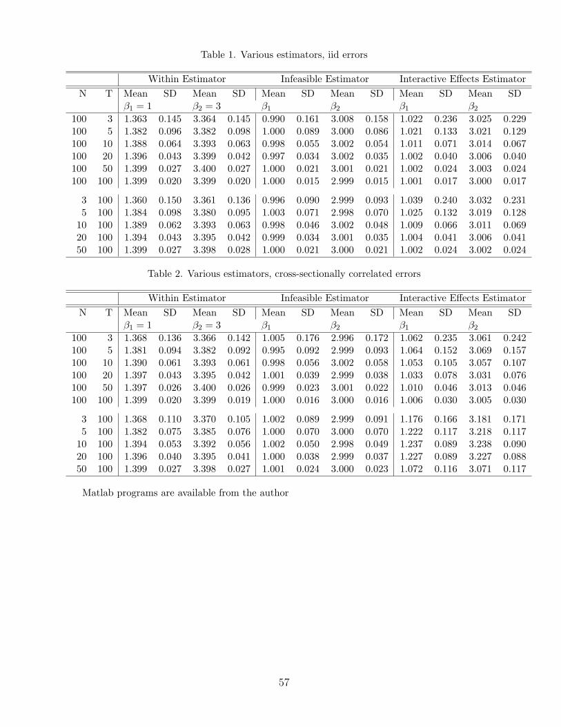
Data are generated according to:

Yit = Xit,1β1 +Xit,2β2 + aλ′iFt + εit

λi = (λi1, λi2)′ and Ft = (Ft1, Ft2). The regressors are generated according to

Xit,1 = µ1 + c1λ′iFt + ι′λi + ι′Ft + ηit,1

Xit,2 = µ2 + c2λ′iFt + ι′λi + ι′Ft + ηit,2

with ι′ = (1, 1). The variables λij, Ftj, ηit,j are all iid N(0, 1). The important parameters are

(β1, β2) = (1, 3).

We set c1 = c2 = µ1 = µ2 = 1 and a = 1. We first consider the case of

εit iid N(0, 4)

then extend to correlated errors.To estimate (βIE, F ), consider the iteration scheme in (9) and (10). A staring value for β or

F is needed. The least squares objective function is not globally convex, there is no guaranteethat an arbitrary starting value will lead to the global optimal solution. Two natural choicesexist. The first is the simple least squares estimator of β, ignoring the interactive effects.The second is the principal components estimator for F , ignoring the regressors. If λi and Ft

have unusually large non-zero means (arbitrarily stretching the model), the first choice can

30

fail, but the second choice leads to the optimal solution. This is because as the interactiveeffects become dominant, it makes sense to estimate the factor structure first. In this case,using the within estimator β as a starting value will also work. To minimize the chance oflocal minimum, both choices are used. Upon convergence, we choose the estimator that givesa smaller value of the objective function. Iterations based on (9) and (10) have difficulty ofachieving convergence for models with time-invariant and common regressors.

A more robust iteration scheme (having much better convergence property) is the following:given F and Λ, compute β(F,Λ) = (

∑Ni=1X

′iXi)

−1∑Ni=1X

′i(Yi−Fλi); and given β, compute F

and Λ from the pure factor model Wi = Fλi + ei with Wi = Yi −Xiβ. This iteration schemeonly requires a single matrix inverse (

∑Ni=1X

′iXi)

−1, no need of updating during iteration,unlike the scheme of β(F ) = (

∑Ni=1X

′iMFXi)

−1∑Ni=1X

′iMFYi. Furthermore, if N > T , we do

principal components analysis using WW ′ (T × T ); and if N < T , we use W ′W (N × N)to speed up computation. They give the same product F λi no matter which matrix is used.For the model associated with Table 4, the iteration method in previous paragraph has manyrealizations not converging to global optimum, but for the iteration scheme here all lead toglobal solution.

For comparison, we also compute two additional estimators: (i) the usual within estimatorβLSDU , (ii) infeasible estimator β(F ), assuming F is observable.

From Table 1, we can draw several conclusions. First, the within estimator is biased andinconsistent. Biases become more severe when the interactive effects are magnified by settinga larger a. For example, if a = 10, the biases are also almost ten times larger (not reported).The infeasible estimator and the interactive effects estimator are virtually unaffected by thevalue of a. Second, both the feasible and interactive effects estimators are unbiased andconsistent. The interactive effects estimator is less efficient than the infeasible estimator, ascan be seen from the larger standard errors, which is consistent with the theory. Third, evenwith small N and T , the interactive effects estimator performs quite well, and both N and Tincreases, the standard deviation becomes smaller.

Table 2 gives results for cross-sectionally correlated εit. For cross-sectional data in reality,a large value of |i− j| does not necessarily mean the correlation between εit and εjt is small.Nevertheless, for the purpose of introducing cross-section correlation, εit is generated as AR(1)for each fixed t such that

εit = ρεi−1,t + eit

where ρ = 0.7. Once cross-section correlation is introduced, the data can be permuted cross-sectionally if wanted, but the results do not depend on any particular permutation. Wegenerate stationary data by discarding the first 100 observations. This implies that var(εit) =σ2

e/(1 − ρ2) ≈ 4 for σ2e = 2 and ρ = 0.7. Thus the variance of εit is approximately the same

as the variance for Table 1. Theorem 5.6 claims that for N >> T , cross-section correlationdoes not affect consistency. On the other hand, for small N (no matter how large is T ), theestimates are inconsistent. In fact, the model is unidentified as explained following equation(6), as long as the cross-section correlation is regarded as having an unknown form. Thesimulation results are consistent with those predictions.

Table 3 reports results when the true model has additive effects such that

λ′iFt = αi + ξt.

Three estimators are computed: (1) the within estimator, which is efficient given additivity,(2) the infeasible estimator, which assumes Ft = (1, ξt)

′ is observed; (3) the interactive ef-

31

fects estimator, which treats the additive effects as if they were interactive effects. Data aregenerated as in Table 1, except that effects are additive. All three estimators are consistent.For small N or small T , the interactive effects estimator shows some bias. These findings areconsistent with the theory.

Table 4 presents results for models with grand mean, time-invariant regressors, commonregressors, and regressors having variations in both dimensions. The model is

Yit = Xit,1β1 +Xit,2β2 + µ+ xiγ + wtδ + λ′iFt + εit

(β1, β2, µ, γ, δ) = (1, 3, 5, 2, 4)

where all variables are generated as in Table 1, and additionally, xi ∼ ι′λi + ei, wt = ι′Ft + ηi,with ei and ηi are iid N(0,1) independent of all other regressors. The within estimator canonly estimate β1 and β2 and is inconsistent (not reported). The cases of very small N or smallT (say T = 3 and T = 5) have convergence problem, we thus consider cases with N and T nosmaller than 10. The infeasible estimators and interactive effects estimators are all consistent,but the latter is less efficient than the former, as expected.

12 Concluding remarks

In this paper, we have derived the rate of convergence and the limiting distribution of theestimated common slope coefficients in panel data models with interactive effects. We showedthat the convergence rate for the interactive-effects estimator is

√NT , and this rate holds

in spite of correlations and heteroskedasticity in both dimensions. We also derived bias cor-rected estimator and estimators under additivity restrictions and their limiting distributions.We further studied the problem testing additive effects against interactive effects. The in-teractive effects estimator is easy to compute, and both the factor process Ft and the factorloadings λi can also be consistently estimated. Under genuine interact effects, we show thatthe grand mean, the coefficients of time-invariant regressors and those of common regressorsare identifiable and can be consistently estimated.

Many important and interesting issues remain to be examined. A useful extension islarge N -large T dynamic panel data model with multiple interactive effects. Another broadextension is nonstationary panel data analysis, particulary panel data cointegration, a subjectthat recently attracts considerable attention. In this setup, Xit is a vector of integratedvariable, and Ft can be either integrated or stationary. When Ft is integrated, then Yit, Xit

and Ft are cointegrated. Neglecting Ft is equivalent to spurious regression and the estimationof β will not be consistent. However, interactive effect approach can be applied by jointlyestimating the unobserved common stochastic trends Ft and the model coefficients, leadingto consistent estimation.

32

Appendix: Proofs

We use the following facts throughout: T−1‖Xi‖2 = T−1∑Tt=1 ‖Xit‖2 = Op(1) or T−1/2‖Xi‖ =

Op(1). Averaging over i, (TN)−1∑Ni=1 ‖Xi‖2 = Op(1). Similarly, T−1/2‖F 0‖ = Op(1), and

T−1‖F‖2 = r, T−1/2‖F‖ =√r, and T−1‖X ′

iF0‖ = Op(1), etc. Throughout, we define δNT =

min[√N,√T ] so that δ2

NT = min[N, T ].

Lemma 12.1 Under assumptions A-D,

supF‖ 1

NT

N∑i=1

X ′iMF εi‖ = op(1)

supF‖ 1

NT

N∑i=1

λ′iF0′MF εi‖ = op(1)

supF‖ 1

NT

N∑i=1

ε′iPF εi‖ = op(1)

where the sup is taken with respect to F such that F ′F/T = I.

Proof. From 1NT

∑Ni=1X

′iεi = op(1), it is sufficient to show supF

1NT

∑Ni=1X

′iPF εi = op(1).

Using PF = FF ′/T ,

1

NT‖

N∑i=1

XiPF εi‖ = ‖ 1

N

N∑i=1

(X ′

iF

T)1

T

T∑t=1

Ftεit‖ ≤1

N

N∑i=1

‖X′iF

T‖ · ‖ 1

T

T∑t=1

Ftεit‖

Note T−1‖X ′iF‖ ≤ T−1‖Xi‖·‖F‖ =

√rT−1/2‖Xi‖ ≤

√r( 1

T

∑Tt=1 ‖Xit‖2)1/2 because T−1/2‖F‖ =√

r. Thus the above is bounded by, using the Cauchy-Schwarz inequality,

√r( 1

N

N∑i=1

1

T

T∑t=1

‖Xit‖2)1/2( 1

N

N∑i=1

‖ 1

T

T∑t=1

Ftεit‖2)1/2

The first expression is Op(1). It suffices to show the second term is op(1) uniformly in F . Now

1

N

N∑i=1

‖ 1

T

T∑t=1

Ftεit‖2 = tr( 1

N

N∑i=1

1

T 2

T∑t=1

T∑s=1

FtF′sεitεis

)

= tr( 1

T 2

T∑t=1

T∑s=1

FtF′s

1

N

N∑i=1

[εitεis − E(εitεis)])

+ tr( 1

T 2

T∑t=1

T∑s=1

FtF′s

1

N

N∑i=1

σii,ts

)where σii,ts = E(εitεis). The first expression is bounded by Cauchy-Schwarz inequality,

( 1

T 2

T∑t=1

T∑s=1

‖Ft‖2‖Fs‖2)1/2

N−1/2( 1

T 2

T∑t=1

T∑s=1

[ 1√N

N∑i=1

[εitεis − E(εitεis)]]2)1/2

But T−1∑Tt=1 ‖Ft‖2 = ‖F ′F/T‖ = r. Thus above is equal to rN−1/2Op(1). Next, | 1

N

∑Ni=1 σii,ts| ≤

τts by Assumption C2. Again by the Cauchy-Schwarz inequality,

‖ 1

T 2

T∑t=1

T∑s=1

FtF′s

1

N

N∑i=1

σii,ts‖ ≤( 1

T 2

T∑t=1

T∑s=1

‖Ft‖2‖Fs‖2)1/2( 1

T 2

T∑t=1

T∑s=1

τ 2ts

)1/2

33

= rT−1/2( 1

T

T∑t=1

T∑s=1

τ 2ts

)1/2= rO(T−1/2)

the last equality follows from τ 2ts ≤ Mτts and Assumption C2. The proof for the remaining

statements are the same, thus omitted. Stock and Watson (2002) have similar results butthey require ‖Ft‖ be bounded uniformly in t, ruling out Ft with unbounded support. Ourproof does not need bounded Ft, nor our optimization with respect to Ft needs to be takenover bounded set.

Proof of Proposition 5.1. Without loss of generality, assume β0 = 0 (purely for notationalsimplicity), and from Yi = Xiβ

0 + F 0λi + εi = F 0λi + εi, expanding SNT (β, F ),

SNT (β, F ) = SNT (β, F ) + 2β′1

NT

N∑i=1

X ′iMF εi + 2

1

NT

N∑i=1

λ′iF0′MF εi +

1

NT

N∑i=1

ε′i(PF − PF 0)εi

where

SNT (β, F ) = β′( 1

NT

N∑i=1

X ′iMFXi

)β + tr[(

F 0′MFF0

T)(

Λ′Λ

N)] + 2β′

1

NT

N∑i=1

X ′iMFF

0λi (40)

By Lemma 12.1SNT (β, F ) = SNT (β, F ) + op(1) (41)

uniformly over bounded β and over F such that F ′F/T = I. Bounded β is in fact notnecessary because the objective funtion is quadratic in β (that is, it is easy to argue that theobjective function cannot achieve its minimum for very large β).

Clearly, SNT (β0, F 0H) = 0 for any r×r invertible H, because MF 0H = MF 0 and MF 0F 0 =0. The identification restrictions implicitly specify a unique H. We next show that for any(β, F ) 6= (β0, F 0H), SNT (β, F ) > 0, thus SNT (β, F ) attains its unique minimum value 0 at(β0, F 0H) = (0, F 0H).

Define

A =1

NT

N∑i=1

X ′iMFXi, B = (

Λ′Λ

N⊗ IT ), C =

1

NT

N∑i=1

(λ′i ⊗MFXi)

and let η = vec(MFF0) then

SNT (β, F ) = β′Aβ + η′Bη + 2β′C ′η

Completing square, we have

SNT (β, F ) = β′(A− C ′B−1C)β + (η′ + β′CB−1)B(η +B−1Cβ)

= β′D(F )β + θ′Bθ

where θ = (η + B−1Cβ). By Assumption A, D(F ) is positive definite, and B is also positivedefinite, so SNT (β, F ) ≥ 0. In addition, if either β 6= β0 = 0 or F 6= F 0H, then SNT (β, F ) > 0.Thus, SNT (θ, F ) achieves its unique minimum at (β0, F 0H). Further, for ‖β‖ ≥ c > 0,SNT (β, F ) ≥ ρminc

2 > 0, where ρmin is the minimum eigenvalue of the positive definite matrixinfF D(F ). This implies that β is consistent for β0 = 0. However, we cannot deduce that F

34

is consistent for F 0H. This is because F 0 is T × 1, and as T → ∞, the number of elementsgoing to infinity, the usual consistency is not a well defined. Other notion of consistency willbe examined.

To prove part (ii), note that the centered objective function satisfies SNT (β0, F 0) = 0, andby definition, SNT (β, F ) ≤ 0. Therefore, in view of (41)

0 ≥ SNT (β, F ) = SNT (β, F ) + op(1).

Combined with SNT (β, F ) ≥ 0, it must be true that

SNT (β, F ) = op(1)

From βp−→ β0 = 0 and (40), it follows that the above implies

tr[F 0′MFF

0

T

Λ′Λ

N] = op(1)

Because Λ′Λ/N > 0, andF 0′MF F 0

T≥ 0, the above implies the latter matrix is op(1), i.e,

F 0′MFF0

T=F 0′F 0

T− F 0′F

T

F ′F 0

T= op(1).

By assumption B, F 0′F 0/T is invertible, it follows that F 0′F /T is invertible.In all remaining proofs, β and β0 are used interchangeably, and so are F and F 0.

Proof of Proposition 5.2. From

[ 1

NT

N∑i=1

(Yi −Xiβ)(Yi −Xiβ)′]F = F VNT

and Yi −Xiβ = Xi(β − β) + F 0λi + εi, expanding terms, we obtain

F VNT =1

NT

N∑i=1

Xi(β − β)(β − β)′X ′iF +

1

NT

N∑i=1

Xi(β − β)λ′iF0′F

+1

NT

N∑i=1

Xi(β − β)ε′iF +1

NT

N∑i=1

F 0λi(β − β)′X ′iF +

1

NT

N∑i=1

εi(β − β)′X ′iF

+1

NT

N∑i=1

F 0λiε′iF +

1

NT

N∑i=1

εiλ′iF

0′F +1

NT

N∑i=1

εiε′iF

+1

NT

N∑i=1

F 0λiλ′iF

0′F

= I1 + · · ·+ I9

The last term on the right is equal to F 0 (Λ′Λ/N)(F 0′F /T ). Let I1, ..., I8 denote the eightterms on the right, the above can be rewritten as

F VNT − F 0 (Λ′Λ/N)(F 0′F /T ) = I1 + · · ·+ I8 (42)

35

Multiplying (F 0′F /T )−1(Λ′Λ/N)−1 on each side of (42)

F [VNT (F 0′F /T )−1(Λ′Λ/N)−1]− F 0 = (I1 + · · ·+ I8)(F 0′F /T )−1(Λ′Λ/N)−1 (43)

Note the matrix VNT (F 0′F /T )−1(Λ′Λ/N)−1 is equal to H−1, but the invertibility of VNT isnot proved yet. We have

T−1/2‖F [VNT (F 0′F /T )−1(Λ′Λ/N)−1]−F 0‖ ≤ T−1/2(‖I1‖+· · · ‖I8‖)‖·‖(F 0′F /T )−1(Λ′Λ/N)−1‖

Consider each term on the right. For the first term, note that T−1/2‖F‖ =√r,

T−1/2‖I1‖ ≤ 1

N

N∑i=1

(‖Xi‖2/T )‖β − β‖2√r = Op(‖β − β‖2) = op(‖β − β‖)

because ‖β − β‖ = op(1). Using the same argument, it is easy to prove next four terms

( I2 to I5) are each Op(β − β). The last three terms do not explicitly depend on β − βand they have the same expressions as those in Bai and Ng (2002). Each of these termsis Op(1/min[

√N,√T ]), which is proved in Bai and Ng (Theorem 1). The proof there only

uses the property that F ′F /T = I, and the assumptions on εi. The proof there needs nomodification. In summary, we have

T−1/2‖F VNT (F 0′F /T )−1(Λ′Λ/N)−1 − F 0‖ = Op(‖β − β‖) +Op(1/min[√N,√T ]). (44)

Proof of part (i). Left multiplying (42) by F ′ and using F ′F = T , we have

VNT − (F ′F 0/T )(Λ′Λ/N)(F 0′F /T ) = T−1F ′(I1 + · · · I8) = op(1)

because T−1/2‖F‖ =√r and T−1/2‖(I1 + · · · I8)‖ = op(1). Thus

VNT = (F ′F 0/T )(Λ′Λ/N)(F 0′F /T ) + op(1)

Proposition 1 shows F ′F 0/T is invertible, thus VNT is invertible. To obtain the limit of VNT ,left multiplying (42) by F 0′ and then dividing by T ,

(F 0′F 0/T )(Λ′Λ/N)(F 0′F /T ) + op(1) = (F 0′F /T )VNT

because T−1F 0′(I1 + ...+ I8) = op(1). The above equality shows that the columns of F 0′F /Tare the (non-normalized) eigenvectors of the matrix (F 0′F 0/T )(Λ′Λ/N), and VNT consists of

the eigenvalues of the same matrix (in the limit). Thus VNTp−→ V , where V is r×r, consisting

of the r eigenvalues of the matrix ΣF ΣΛ.Proof of part (ii). Since VNT is invertible, the left side (44) can be written as T−1/2‖FH−1−

F 0‖, thus (44) is equivalent to

T−1/2‖F − F 0H‖ = Op(‖β − β‖) +Op(1/min[√N,√T ])

Taking squares on each side gives part (ii). Note the cross product term from expanding thesquares has the same bound.

36

Lemma 12.2 Under assumptions A-C, there exist an M <∞, such that(i)

E‖N−1/2N∑

k=1

1

T

T∑t=1

T∑s=1

FsF′t [εktεks − E(εktεks)]‖2 ≤M

(ii) for all i = 1, 2..., N and h = 1, 2, ..., r,

E‖N−1/2N∑

k=1

1

T

T∑t=1

T∑s=1

Xit[εktεks − E(εktεks)]Fhs

‖2 ≤M

Proof of (i). Denote the term inside ‖ · ‖2 as A. Then the left hand side is equal to Etr(AA′).Using E‖Ft‖4 ≤M and Assumption C.4, (i) follows readily. The proof of (ii) is similar.

Lemma 12.3 Under assumptions of Proposition 5.3,

(i) T−1F 0′(F − F 0H) = Op(β − β) +Op(δ−2NT )

(ii) T−1F ′(F − F 0H) = Op(β − β) +Op(δ−2NT )

(iii) T−1X ′k(F − F 0H) = Op(β − β) +Op(δ

−2NT ), for each k = 1, 2, ..., N .

(iv) 1NT

∑Ni=1X

′iMF (F − F 0H) = Op(β − β) +Op(δ

−2NT )

Proof of (i). This part extends Lemma B.2 of Bai (2003). Using (43), it is easy to see thatthe first five terms are each Op(β − β). In fact, the first, third and fifth are op(β − β), the

second and fourth are Op(β−β). The next three terms are considered in Bai (2003) and eachis shown to be Op(δ

−2NT ) in the absence of β. With the estimation of β, they are each to be

Op(β − β)Op(δ−1NT ) +Op(δ

−2NT ) due to Proposition 5.2(ii) instead of Lemma A.1 of Bai (2003).

But Op(β − β)Op(δ−1NT ) is dominated by Op(β − β), the order of the first five terms. Thus

summing over the eight terms, we obtain part (i).For part (ii),

‖T−1F ′(F − F 0H‖ ≤ T−1‖F − F 0H‖2 + ‖H‖T−1‖F 0′(F − F 0H)‖ = Op(β − β) +Op(δ−2NT )

by part (i) and Proposition 5.2(ii). The proof of part (iii) is identical to part (i).For (iv)

1

NT

N∑i=1

X ′iMF (F − F 0H) =

1

N

N∑i=1

1

TX ′

i(F − F 0H) +1

N

N∑i=1

X ′iF

TF ′(F − F 0H)

The first term on the right is an average of (iii) over i, and thus is still that order of magnitude.The second term is bounded by 1

N

∑Ni=1 ‖Xi/

√T‖2

√r‖T−1F ′(F −F 0H)‖ = Op(1)‖T−1F ′(F −

F 0H)‖. Thus (iv) follows from part (ii).

Lemma 12.4 Under assumptions of Proposition 3,(i) T−1ε′k(F − F 0H) = T−1/2Op(β − β) +Op(δ

−2NT ), for each k.

(ii) 1T√

N

∑Nk=1 ε

′k(F − F 0H) = T−1/2Op(β − β) +N−1/2Op(β − β) +Op(N

−1/2) +Op(δ−2NT ).

(iii) 1NT

∑Nk=1 λ

′k(FH

−1 − F 0)′εk = (NT )−1/2Op(β − β) +Op(N−1) +N−1/2Op(δ

−2NT )

(iv)

1

NT

N∑k=1

X ′kF

0

T(F 0′F 0

T)(FH−1 − F 0)′εk =

1

N2

N∑i=1

N∑k=1

X ′kF

0

T(F 0′F 0

T)(Λ′Λ/N)−1λi

( 1

T

T∑t=1

εitεkt

)+(NT )−1/2Op(β − β) +N−1/2Op(δ

−2NT )

37

Proof of (i). Part (i) extends lemma B.1 of Bai (2003). The proof is omitted as it is easierthan the proof part (ii) (a proof can be found in a working version). Now consider the proofof (ii). From (43) and denoting G = (F 0′F /T )−1(Λ′Λ/N)−1 for the moment

T−1N−1/2N∑

k=1

ε′k(FH−1 − F 0) = T−1N−1/2

N∑k=1

ε′k(I1 + · · ·+ I8)G = a1 + · · ·+ a8

We show that first four terms are each T−1/2Op(β − β).

‖a1‖ ≤ T−1/2‖G‖(

1

N

N∑i=1

‖( 1√TN

N∑k=1

T∑t=1

εktXit)‖(‖Xi‖2/T )

)‖β−β‖2 = T−1/2‖β−β)‖2Op(1)

a2 =1

NT

1√N

N∑k=1

N∑i=1

ε′kXi(β−β)λi(Λ′Λ/N)−1 =

1√T

1

N

N∑i=1

1√NT

N∑k=1

T∑t=1

XitεktOp(β−β)λi(Λ′Λ/N)−1

= T−1/2(β − β)

‖a3‖ ≤ T−1/2‖G‖(

1

N

N∑i=1

‖ 1√NT

N∑k=1

T∑t=1

εktXit‖(‖εi‖2/T )‖)β − β‖ = T−1/2Op(‖β − β‖)

a4 = T−1/2(1√NT

N∑k=1

T∑t=1

εktF′t)(β − β)′

(1

N

N∑i=1

(X ′iF /T )

)G = T−1/2Op(β − β)

For a5, let Wi = X ′iF /T , note that ‖Wi‖2 ≤ ‖Xi‖2/T ,

a5 =1

NT

1√N

N∑k=1

N∑i=1

ε′kεi(β − β)′WiG

=1√N

1

T

T∑t=1

(1√N

N∑k=1

εkt)(1√N

N∑i=1

εit(β − β)Wi)G = N−1/2Op(β − β)

For a6,

a6 =1

NT 2

1√N

N∑k=1

ε′kF0

N∑i=1

λiε′iFG =

1

NT 2

1√N

N∑k=1

ε′kF0

N∑i=1

λiε′iF

0HG

+1

NT 2

1√N

N∑k=1

ε′kF0

N∑i=1

λiε′i(F − F 0H)G = a6.1 + a6.2

a6.1 =1√NT

( 1√NT

N∑k=1

T∑t=1

F 0′t εkt

)( 1√NT

N∑i=1

T∑t=1

λiF0′t εit

)HG = Op(T

−1N−1/2)

a6.2 = T−1/2( 1√

NT

N∑k=1

T∑t=1

F 0′t εkt

) 1

TN

N∑i=1

λiε′i(F − F 0H)G

‖a6.2‖ ≤ T−1/2Op(1)1

N

N∑i=1

‖λi‖|εi/√T‖‖F − F 0H‖√

T‖G‖

= T−1/2[Op(β − β) +Op(δ−1NT )] = T−1/2(β − β) +Op(δ

−2NT )

38

Next consider a7.

a7 =1

NT

1√N

N∑k=1

N∑i=1

ε′kεiλ′i(Λ

′Λ/N)−1

= N−1/2 1

T

T∑t=1

[(

1√N

N∑k=1

εkt)(1√N

N∑i=1

εitλ′i)](Λ′Λ/N)−1 = Op(N

−1/2)

a8 =1

NT 2

1√N

N∑k=1

N∑i=1

ε′kεi(ε′iF )G =

1

NT 2

1√N

N∑k=1

N∑i=1

ε′kεi(ε′iF

0)HG+1

NT 2

1√N

N∑k=1

N∑i=1

ε′kεi(ε′i(F−F 0H))G

= b8 + c8

b8 =1

NT

N∑i=1

[( 1√TN

N∑k=1

T∑t=1

(εktεit − E(εktεit))( 1√

T

T∑s=1

εisF0sH

)]G

+1√NT

1

NT

N∑k=1

N∑i=1

T∑t=1

γki,t1√T

T∑s=1

εisF0sHG = Op(T

−1) +Op((NT )−1/2)

Ignore G,

c8 = T−1/2 1

N

N∑i=1

1√TN

N∑k=1

T∑t=1

[εktεit−E(εktεit)]ε′i(F − F 0H)

T+

1

N3/2T

N∑k=1

N∑i=1

T∑t=1

γki,tε′i(F − F 0H)

T

= c8.1 + c8.2

‖c8.1‖ ≤ T−1/2( 1

N

N∑i=1

[ 1√TN

N∑k=1

T∑t=1

[εktεit−E(εktεit)]2)1/2( 1

N

N∑i=1

‖εi‖2/T ))1/2

‖F−F 0H‖/√T

= T−1/2Op(‖β − β‖) + T−1/2Op(δ−1NT ) = T−1/2Op(‖β − β‖) +Op(δ

−2NT )

‖c8.2‖ ≤ 1√N

‖F − F 0H‖√T

1

N

N∑k=1

N∑i=1

‖γki‖εi‖/√T

= [Op(‖β − β‖) +Op(δ−1NT )]N−1/2 = N−1/2Op(‖β − β‖) +Op(δ

−2NT )

Note that EN−1∑Nk=1

∑Ni=1 ‖γki‖εi‖/

√T ≤ maxiE(‖εi‖/

√T )N−1∑N

k=1

∑Ni=1 |γki| = O(1).

Part (iii) is derived from (ii) with the division by√N . The presence of λk does not alter

the results. A direct proof would be similar to that of (ii). The details are omitted.Part (iv) is the same as (iii) with λk replaced by (X ′

kF0/T )(F 0′F 0/T ) = Op(1). The first

term on the right is an elaboration of the corresponding Op(N−1) term appearing in (iii). This

elaborated expression will be used later.

Proof of Proposition 5.3. From Yi = Xiβ0 + F 0λi + εi

β − β0 = (N∑

i=1

X ′iMFXi)

−1N∑

i=1

X ′iMFF

0λi + (N∑

i=1

X ′iMFXi)

−1N∑

i=1

X ′iMF εi

or

(1

NT

N∑i=1

X ′iMFXi)(β − β) =

1

NT

N∑i=1

X ′iMFF

0λi +1

NT

N∑i=1

X ′iMF εi (45)

39

In view of MF F = 0, we have MFF0 = MF (F 0 − FA) for any A. Choose A = H−1, from

(43),F 0 − FH−1 = −[I1 + · · · I8](F 0′F /T )−1(Λ′Λ/N)−1

It follows that

1

NT

N∑i=1

X ′iMFF

0λi = − 1

NT

N∑i=1

X ′iMF

[I1 + · · ·+ I8

](F 0′F /T )−1(Λ′Λ/N)−1λi

= J1 + · · ·+ J8

where J1 up to J8 are implicitly defined vis-a-vis I1− I8. For example,

J1 = − 1

NT

N∑i=1

X ′iMF (I1)(F 0′F /T )−1(Λ′Λ/N)−1λi

Term J1 is bounded in norm by Op(1)‖β − β‖2 and thus J1 = op(1)(β − β). Consider J2.

J2 = − 1

N2T

N∑i=1

X ′iMF

[ N∑k=1

Xk(β − β)λ′k(Λ′Λ/N)−1

]λi

=1

N2T

N∑i=1

N∑k=1

(X ′iMFXk)[λ

′k(Λ

′Λ/N)−1λi](β − β)

=1

T

[ 1

N

1

N

N∑i=1

N∑k=1

X ′iMFXkaik

](β − β)

where aik = λ′i(Λ′Λ/N)−1λk is a scalar and thus commutable with β − β.

J3 =1

N2T

N∑i=1

N∑k=1

X ′iMFXk(ε

′kF /T )(F ′F 0/T )−1(Λ′Λ/N)−1λi(β − β)

Write ε′kF /T = ε′kF0H/T + ε′k(F −F 0H)/T = Op(T

−1/2)+Op(β−β)+Op(1/min[√N,√T ]),

by Lemma 12.4, it easy to see J3 = op(1)(β − β).Next

J4 = − 1

N2T

N∑i=1

N∑k=1

X ′iMFF

0λk(β − β)′(X ′kF /T )(F ′F 0/T )−1(Λ′Λ/N)−1λi

Write MFF0 = MF (F 0 − FH−1) and using T−1/2‖F 0 − FH−1‖ being small, J4 is equal to

op(1)(β − β). It is easy to show J5 = op(1)(β − β) and thus omitted.

The last three terms J6-J8 do not explicitly depend on β − β. Only term J7 contributesto the limiting distribution of β − β, the other two terms are op((NT )−1/2) plus op(β − β).We shall establish these claims. Consider J6.

J6 = − 1

N2T

N∑i=1

N∑k=1

X ′iMFF

0λk(ε′kF /T )(F ′F 0/T )−1(Λ′Λ/N)−1λi

40

Denote G = (F ′F 0/T )−1(Λ′Λ/N)−1 for a moment, it is a matrix of fixed dimension, and doesnot vary with i. Using MFF

0 = MF (F 0 − FH−1),

J6 = − 1

NT

N∑i=1

X ′iMF (F 0 − FH−1)

( 1

N

N∑k=1

λk(ε′kF /T )

)Gλi

Now1

NT

N∑k=1

λkε′kF =

1

NT

N∑k=1

λkε′kF

0H +1

NT

N∑k=1

λkε′k(F − F 0H)

= Op(1√NT

) + (NT )−1/2Op(β − β) +Op(N−1) +N−1/2Op(δ

−2NT )

= Op(1√NT

) +Op(N−1) +N−1/2Op(δ

−2NT )

by Lemma 12.4(iii). The last equality is because (NT )−1/2 dominates (NT )−1/2(β − β).Furthermore, by Lemma 12.3 1

NT

∑Ni=1X

′iMF (F − F 0H)λi` = Op(β − β) + Op(δ

−2NT ) for ` =

1, 2, ..., r, and noting G does not depend on i and ‖G‖ = Op(1), we have

J6 =[Op(β − β) +Op(δ

−2NT )

][Op(

1√NT

) +Op(N−1) +N−1/2Op(δ

−2NT )

]

= op(β − β) + op(1√NT

) +Op(δ−2NT )N−1 +N−1/2Op(δ

−4NT ).

The term J7 is simply

J7 = − 1

N2T

N∑i=1

X ′iMF

[ N∑k=1

εkλ′k(Λ

′Λ/N)−1]λi = − 1

N2T

N∑i=1

N∑k=1

aikX′iMF εk.

Next consider J8, which has the expression

J8 = − 1

N2T 2

N∑i=1

N∑k=1

X ′iMF εkε

′kF (F 0′F /T )−1(Λ′Λ/N)−1λi

Let E(εkε′k) = Ωk, a T × T matrix. Denote G = (F 0′F /T )−1(Λ′Λ/N)−1, ‖G‖ = Op(1).

Rewrite

J8 = − 1

N2T 2

N∑i=1

N∑k=1

X ′iMF ΩkFGλi −

1

N2T 2

N∑i=1

N∑k=1

X ′iMF (εkε

′k − Ωk)FGλi (46)

When no serial correlation and heteroskedasticity, Ωk = σ2kIT . From MF F = 0, the first term

is equal to zero. The second term being small does not rely on Ωk = σ2kIT . Lemma 12.5 below

deals with general Ωk that will also be applicable for Proposition 5.5. By Lemma 12.5, wehave

J8 = Op(1

T√N

) + (NT )−1/2[Op(β − β) +Op(δ−1NT )] +

1√NOp(‖β − β‖2) +

1√NOp(δ

−2NT ).

41

Collecting terms from J1 to J8 with dominated terms ignored,

1

NT

N∑i=1

X ′iMFF

0λi

= J2 + J7 + op(β − β) + op((NT )−1/2) +Op(1

T√N

) +N−1/2Op(δ−2NT )

Thus, ( 1

NT

N∑i=1

X ′iMFXi + op(1)

)(β − β)− J2 =

1

NT

N∑i=1

XiMF εi + J7

+op((NT )−1/2) +Op(1

T√N

) +N−1/2Op(δ−2NT )

Combining terms and multiplying√NT

[D(F ) + op(1)

]√NT (β − β) =

1√NT

N∑i=1

[X ′

iMF −1

N

N∑k=1

aikX′kMF

]εi + op(1)

+Op(T−1/2) + T 1/2Op(δ

−2NT )

Thus, if T/N2 → 0, the last term is also op(1). Noting [D(F ) + op(1)]−1 = D(F )−1 + op(1),

we proved the proposition.

Lemma 12.5 Under the assumptions of Proposition 5.3 and for G = (F 0′F /T )−1(Λ′Λ/N)−1

1

N2T 2

N∑i=1

N∑k=1

X ′iMF (εkε

′k − Ωk)FGλi

= Op(1

T√N

) + (NT )−1/2[Op(β − β) +Op(δ−1NT )] +

1√NOp(‖β − β‖2) +

1√NOp(δ

−2NT ).

Proof: Rewrite the left hand side as

1

N2T 2

N∑i=1

N∑k=1

X ′i(εkε

′k − Ωk)FGλi −

1

N

N∑i=1

(X ′

iF

T)

1

NT 2

N∑k=1

F ′(εkε′k − Ωk)FGλi = I + II

Adding and subtracting terms

I =1

N2T 2

N∑k=1

N∑i=1

X ′i(εkε

′k − Ωk)F

0HGλi +1

N2T 2

N∑k=1

N∑i=1

X ′i(εkε

′k − Ωk)(F − F 0H)Gλi

The first term on the right is equal to

(1

N2T 2)

N∑i=1

N∑k=1

T∑t=1

T∑s=1

Xit[εktεks − E(εktεks)]F0′s HGλi

=1

T√N

1

N

N∑i=1

[N−1/2

N∑k=1

1

T

T∑t=1

T∑s=1

Xit[εktεks − E(εktεks)]F0′s

]HGλi = Op(

1

T√N

)

42

by Lemma 12.2(ii). Denote

as =( 1√

NT

N∑k=1

T∑t=1

Xit[εktεks − E(εktεks)])

= Op(1)

Then the second term of I is

1√NT

1

N

N∑i=1

1

T

T∑s=1

as(Fs − F 0sH)

‖ 1

T

T∑s=1

as(Fs − F 0sH)‖ ≤ (

1

T

T∑s=1

‖as‖2)1/2(1

T

T∑s=1

‖Fs − F 0sH‖2)1/2 = Op(β − β) +Op(δ

−1NT )

Thus the second term of I is (NT )−1/2[Op(β − β) +Op(δ−1NT )]. Consider II.

‖II‖ ≤ 1

N

N∑i=1

‖XiF

T‖‖Gλi‖ · ‖

1

NT 2

N∑k=1

F ′(εkε′k − Ωk)F‖ = Op(1)‖

1

NT 2

N∑k=1

F ′(εkε′k − Ωk)F‖

But

1

NT 2

N∑k=1

F ′(εkε′k − Ωk)F

= H1

NT 2

N∑k=1

F 0′(εkε′k − Ωk)F

0H

+H1

NT 2

N∑k=1

F 0′(εkε′k − Ωk)(F − F 0H)

+1

NT 2

N∑k=1

(F − F 0H)′(εkε′k − Ωk)F

0H

+1

NT 2

N∑k=1

(F − F 0H)′(εkε′k − Ωk)(F − F 0H)

= b1 + b2 + b3 + b4

Now

b1 = H(1

T 2N)

N∑k=1

T∑t=1

T∑s=1

FsF′t [εktεks − E(εktεks)]H = Op(

1

T√N

)

by Lemma 12.2(i). Next

b2 = H1√NT

1

T

T∑s=1

[ 1√NT

T∑t=1

N∑k=1

F 0t [εktεks − E(εktεks)]

](Fs −H ′F 0

s )

Thus if we let As = 1√NT

∑Tt=1

∑Nk=1 F

0t [εktεks − E(εktεks)],

‖b2‖ ≤ ‖H‖ 1√NT

( 1

T

T∑s=1

‖As‖2)1/2( 1

T

T∑s=1

‖Fs −H ′F 0s ‖2

)1/2=

1√NT

[Op(‖β − β‖) +Op(δ−1NT )]

43

The term b3 has the same upper bound because it is the transpose of b2. The last term

b4 =1√N

1

T 2

T∑t=1

T∑s=1

(Ft −H ′F 0t )(Fs −H ′F 0

s )′[1√N

N∑i=1

[εktεks − E(εktεks)]

Thus by the Cauchy-Schwarz inequality,

‖b4‖ ≤ 1√N

(1

T

T∑t=1

‖Ft −H ′F 0t ‖2)

( 1

T 2

T∑t=1

T∑s=1

[ 1√N

N∑i=1

[εktεks − E(εktεks)]]2)1/2

=1√NOp(‖β − β‖2) +

1√NOp(δ

−2NT ).

Now collecting terms yields the lemma.

Lemma 12.6 Under the assumptions of Proposition 5.4,

HH ′ = (F 0′F 0/T )−1 +Op(‖β − β‖) +Op(δ−2NT )

Proof: The first two results of Lemma 12.3 can be rewritten as

F 0′F /T − (F 0′F 0/T )H = Op(‖β − β‖) +Op(δ−2NT ), and

I − (F ′F 0/T )H = Op(‖β − β‖) +Op(δ−2NT )

Left multiply the first equation by H ′ and use the transpose of the second equation to obtain

I −H ′(F 0′F 0/T )H = Op(‖β − β‖) +Op(δ−2NT )

Right multiplying by H ′ and left multiplying by H ′−1, we obtain

I − (F 0′F 0/T )HH ′ = Op(‖β − β‖) +Op(δ−2NT )

This is equivalent to the lemma.

Lemma 12.7 Under the assumptions of Proposition 5.4,

‖PF − PF 0‖2 = Op(‖β − β‖) +Op(δ−2NT )

Proof‖PF − PF 0‖2 = tr[(PF − PF 0)2] = 2tr(Ir − F ′PF 0F /T ).

Proposition 5.1(ii) already implies Ir−F ′PF 0F /T = op(1). By rewriting T−1F ′F 0 = T−1F (F 0−FH−1)+H, we can easily show using earlier lemmas Ir−F ′PF 0F /T = Op(‖β−β‖)+Op(δ

−2NT ).

The details are omitted.

Proof of Proposition 5.4. We first show D(F )−D(F 0) = op(1).

D(F )−D(F 0) =1

NT

N∑i=1

X ′i(MF −MF 0)Xi −

1

T

[ 1

N2

N∑i=1

N∑k=1

X ′i(MF −MF 0)Xkaik

]

44

The norm of the first term on the right is bounded by

‖ 1

NT

N∑i=1

X ′i(PF − PF 0)Xi‖ ≤

1

N

N∑i=1

(‖Xi‖2/T )‖PF − PF 0‖ = op(1)

by Lemma 12.7. The proof for the second term is op(1) is the same.Much more involved is the proof of the following.

1√NT

N∑i=1

[X ′

iMF −1

N

N∑k=1

aikX′kMF

]εi =

1√NT

N∑i=1

[X ′

iMF 0 − 1

N

N∑k=1

aikX′kMF 0

]εi + op(1)

The above is implied by the following two results, as T/N → 0,

1√NT

N∑i=1

Xi(MF 0 −MF )εi =1√NT

N∑i=1

X ′i(PF − PF 0)εi = op(1) (47)

1√NT

N∑i=1

1

N

N∑k=1

aikX′k(MF 0 −MF )εi = op(1) (48)

Consider (47). By adding and subtracting terms

1√NT

N∑i=1

X ′iF

TF ′εi −

1√NT

N∑i=1

X ′iPF 0εi

=1√NT

N∑i=1

X ′i(F − F 0H)

TH ′F 0′εi +

1√NT

N∑i=1

X ′i(F − F 0H)

T(F − F 0H)′εi

+1√NT

N∑i=1

X ′iF

0H

T(F − F 0H)′εi +

1√NT

N∑i=1

X ′iF

0

T

[HH ′ − (F 0′F 0/T )−1

]F 0′εi

= a+ b+ c+ d

Consider (a). Note (Fs −H ′F 0s )′H ′F 0

t is scalar thus commutable with Xit.

a =1

T

T∑s=1

(Fs −H ′F 0s )′H ′

( 1√NT

N∑i=1

T∑t=1

F 0t Xisεit

)Thus

‖a‖ ≤[ 1

T

T∑s=1

‖Fs −H ′F 0s ‖2

]1/2‖H‖

[ 1

T

T∑s=1

‖( 1√

NT

N∑i=1

T∑t=1

F 0t Xisεit

)‖2]1/2

= [Op(‖β − β‖) +Op(δ−1NT )]Op(1) = op(1)

Similarly,

b = T 1/2 1

T 2

T∑s=1

T∑t=1

(Fs −H ′F 0s )′(Ft −H ′F 0

t )( 1√

N

N∑i=1

Xisεit

)By the Schwarz inequality

‖b‖ ≤√T (

1

T

T∑t=1

‖Ft −H ′Ft‖2)( 1

T 2

T∑s=1

T∑t=1

‖ 1√N

N∑i=1

Xitεit‖2)1/2

45

=√T [Op(‖β − β‖2) +Op(δ

−2NT )]Op(1)

which is op(1) if T/N2 → 0.Consider c.

c =1√NT

N∑i=1

X ′iF

0

THH ′(FH−1 − F 0)′εi =

1√NT

N∑i=1

X ′iF

0

T

(F 0′F 0

T

)−1(FH−1 − F 0)′εi

+1√NT

N∑i=1

X ′iF

0

T

[HH ′ − (

F 0′F 0

T)−1

](FH−1 − F 0)′εi = c1 + c2

Denote Q = HH ′ − (F 0′F 0

T)−1 for the moment. We show c2 = op(1).

c2 =√NT

( 1

NT

N∑i=1

[ε′i(FH−1 − F 0)⊗ (X ′

iF0/T )]

)vec(Q)

=√NT

[(NT )−1/2(‖β − β)‖+Op(N

−1) +N−1/2Op(δ−2NT )

]vec(Q)

by the argument of Lemma 12.4(iii) and (iv). By Lemma 12.6, vec(B) = Op(‖β − β‖) +

Op(δ−2NT ). Thus c2 = Op(β − β) +

√T/NOp(δ

−2NT ) +

√TOp(δ

−4NT )

p−→ 0 if T/N3 → 0.

By Lemma 12.4 (iv), switching the role of i and k,

c1 = (√NT/N)ψNT +Op(β − β) +

√TOp(δ

−2NT )

where

ψNT =1

N

N∑i=1

N∑k=1

X ′iF

0

T

(F 0′F 0

T

)−1(Λ′Λ

N)−1λk(

1

T

T∑t=1

εitεkt) (49)

But ψNT = Op(1) because

ψNT =1

T

T∑t=1

(N−1/2

N∑i=1

Aiεit

)(N−1/2

N∑k=1

Bkεkt

)= Op(1)

with Ai = (X ′iF0/T )(F 0′F 0/T )−1 and Bk = (Λ′Λ/N)−1λk. Thus c1 → 0 if T/N → 0.

For (d), again let Q = HH ′ − (F 0′F 0/T )−1. Then

d =1√NT

N∑i=1

[ε′iF0⊗(X ′

iF0/T )]vec(Q) =

( 1√NT

N∑i=1

T∑t=1

F 0t εit⊗(X ′

iF0/T )

)vec(Q) = Op(1)vec(Q)

which is op(1) because vec(Q) = Op(‖β − β‖) +Op(δ−2NT ) by Lemma 12.6. In summary, ignore

dominated terms

1√NT

N∑i=1

X ′i(MF 0 −MF )εi = (

√NT/N)ψNT +Op(β − β) +

√TOp(δ

−2NT ) (50)

with ψNT = Op(1) being defined in (49). The above is op(1) if T/N → 0, proving (47).It remains to prove (48). This is obtained by replacing Xi in the earlier proof with Vi =

1N

∑Nk=1 aikXk. Then (48) becomes

1√NT

N∑i=1

V ′i (MF 0 −MF )εi = (

√NT/N)ψ∗NT +Op(β − β) +

√TOp(δ

−2NT ) (51)

46

where ψ∗NT = Op(1) is defined as

ψ∗NT =1

N

N∑i=1

N∑k=1

V ′i F

0

T

(F 0′F 0

T

)−1(Λ′Λ

N)−1λk(

1

T

T∑t=1

εitεkt) (52)

Thus (51) is op(1) if T/N → 0.

Proof of Proposition 5.5. In the presence of serial correlation or heteroskedasticity, thefirst term of (46) is no longer zero. Except for this special term, the proof of preceding twopropositions is still valid under serial correlation or heteroskedasticity. Ignore that term for amoment, the proof of Proposition 5.4 shows, combining (50) and (51),

√NT (β − β) = D(F 0)−1 1√

NT

N∑i=1

Z ′iεi +√T/NξNT +Op(β − β) +

√TOp(δ

−2NT )

where

ξNT = −D(F 0)−1(ψNT − ψ∗NT )

= −D(F 0)−1 1

N

N∑i=1

N∑k=1

(Xi − Vi)′F 0

T

(F 0′F 0

T

)−1(Λ′Λ

N)−1λk(

1

T

T∑t=1

εitεkt)

As argued earlier, ξNT = Op(1). Thus if T/N = O(1), then√NT (β − β) = Op(1).

In the presence of serial correlation or time series heteroskedasticity, MF ΩkF 6= 0, sothe first term on the right of (46) is nonzero. Denote that term by ANT . This means that√NT (β − β) has an extra term D(F 0)−1

√NTANT . That is,

√NT (β − β) = D(F 0)−1 1√

NT

N∑i=1

Z ′iεi +√T/NξNT +D(F 0)−1

√NTANT + op(1)

where

ANT = − 1

NT 2

N∑i=1

X ′iMF (

1

N

N∑k=1

Ωk)FGλi = − 1

NT 2

N∑i=1

X ′iΩFGλi +

1

NT 2

N∑i=1

X ′iF

T(F ′ΩF )Gλi

(53)and Ω = 1

N

∑Nk=1 Ωk. We now show that ANT = Op(1/T ) so that

√NTANT = Op((N/T )1/2),

which is Op(1) when N/T is bounded. Note that ‖F ′ΩF‖ ≤ λmax(Ω)‖F ′F‖ = λmax(Ω)rT =O(T ), where λmax(Ω) is the largest eigenvalue of Ω and is bounded by assumption. Thus,Similarly, ‖X ′

iΩF‖ ≤ 12λmax(Ω)[‖Xi‖2 + ‖F‖2].

‖ 1

NT 2

N∑i=1

X ′iΩFGλi‖ ≤

1

2Tλmax(Ω)

( 1

N

N∑i=1

(‖Xi‖2/T + r)‖G‖‖λi‖)

= Op(1/T )

‖ 1

NT 2

N∑i=1

X ′iF

T(F ′ΩF )Gλi‖ ≤

1

Tr3/2λmax(Ω)

(‖ 1

N

N∑i=1

‖Xi‖√T‖G‖‖λi‖

)= Op(1/T )

This completes the proof of Proposition 5.5.Proof of Theorem 5.6. This follows immediately from Proposition 5.4 and Assumption F.

47

Proof of Theorem 5.8. The proof of Proposition 5.4 shows that

√NT (β − β0) = D(F 0)−1 1√

NT

N∑i=1

Z ′iεi +√T/NξNT + op(1) (54)

where ξNT is defined in (15). The expected value of ξNT is given

B = −D(F 0)−1 1

N

N∑i=1

N∑k=1

(Xi − Vi)′F 0

T

(F 0′F 0

T

)−1(Λ′Λ

N)−1λkσ

2ik

We show√T/N(ξNT−B) = op(1). LetAik = λ′k⊗[(Xi−Vi)

′F 0/T ] andG = (F 0′F 0/T )−1(Λ′Λ/N)−1,

then E‖Aik‖2 ≤M and ‖G‖ = Op(1). We have

D(F 0)[ξNT −B] = − 1

N

N∑i=1

N∑k=1

[Aik

1

T

T∑t=1

(εitεkt − σ2ik)]vec(G)

Assumption C4 implies the above is Op(T−1/2). Thus

√T/N(ξNT − B) = Op(N

−1/2) does

not affect the limiting distribution. Since√T/N → √

ρ and plimB = B0 by assumption, thetheorem follows.

Biased correction

Lemma 12.8

(i) 1N‖Λ′ −H−1Λ′‖2 = 1

N

∑Ni=1 ‖λi −H−1λi‖2 = Op(‖β − β‖2) +Op(δ

−2NT ).

(ii) N−1(Λ′ −H−1Λ′

)Λ = Op(‖β − β‖) +Op(δ

−2NT )

(iii) Λ′Λ/N −H−1(Λ′Λ/N)H ′−1 = Op(‖β − β‖) +Op(δ−2NT ).

(iv) (Λ′Λ/N)−1 −H ′(Λ′Λ/N)−1H = Op(‖β − β‖) +Op(δ−2NT ).

Proof: By definition, Λ′ = 1TF ′(Y −Xβ), where Y = (Y1, ..., YN) is T ×N and X is T ×N×p

(three dimensional matrix), so that Xβ is T ×N (readers may consider β is a scalar so thatX is simply T ×N). Thus from Y −Xβ = F 0Λ′ + ε−X(β − β0),

Λ′ = T−1F ′F 0Λ′ + T−1F ′ε− T−1F ′X(β − β0)

From F 0 = F 0 − FH−1 + FH−1 and use F ′F /T = I, we have

Λ′ −H−1Λ′ = T−1F ′(F 0 − FH−1)Λ′ + T−1F ′ε− T−1F ′X(β − β) (55)

Thus

N−1/2‖Λ′ −H−1Λ′‖ ≤√r‖F 0 − FH−1‖√

T

‖Λ‖√N

+ T−1/2‖ 1√NT

F ′ε‖+√r‖X‖√NT

‖β − β‖

The first term is Op(‖β − β‖) + Op(δ−1NT ) by Proposition 5.2(ii), and the second term is

Op(T−1/2), third term is Op(‖β−β‖) in view ‖X‖/

√NT = Op(1). Thus N−1/2‖Λ′−H−1Λ′‖ =

Op(‖β − β‖) +Op(δ−1NT ). This is equivalent to (i).

48

For (ii), left multiplying Λ on each side and then dividing by N ,

N−1(Λ′ −H−1Λ′)Λ = T−1F ′(F 0 − FH−1)(Λ′Λ/N) + (TN)−1F ′εΛ− (TN)−1F ′X(β − β)Λ

The first term on the right is Op(‖β − β‖) +Op(δ−2NT ) by Lemma 12.3. The second term is

(TN)−1(F − F 0H)′εΛ + (TN)−1HF 0′εΛ = a+ b

But (a) is the left hand side of Lemma 12.4(iii), thus having the desired result. Term (b) issimply (TN)−1/2Op(1), also as desired. Finally,

‖(TN)−1F ′X(β − β)Λ‖ ≤√r‖X/

√TN‖ · ‖Λ/

√N‖ · ‖β − β‖ = Op(‖β − β‖)

proving (ii). For (iii), adding and subtracting terms, (iii) follows from (i) and (ii). For (iv)follows from A−1 −B−1 = A−1(B − A)B−1 and (iii).

Lemma 12.9 Under assumptions of Theorem 7.1, for B and B defined in (16) and (17),√T/N(B −B) = op(1)

Proof: The denominator of B isD(F 0). Equation (60) shows that√T/N [D0−D(F 0)] = op(1).

Thus it is sufficient to consider the numerator only. We shall prove

(√T/N)

[1

N

N∑i=1

X ′iF

T(Λ′Λ

N)−1λiσ

2i −

1

N

N∑i=1

X ′iF

0

T

(F 0′F 0

T

)−1(Λ′Λ

N)−1λiσ

2i

]= op(1) (56)

and

(√T/N)

[1

N

N∑i=1

V ′i F

T(Λ′Λ

N)−1λiσ

2i −

1

N

N∑i=1

V ′i F

0

T

(F 0′F 0

T

)−1(Λ′Λ

N)−1λiσ

2i

]= op(1) (57)

Consider (56). There are four items being estimated, namely, F , Λ′Λ/N , λi, and σ2i . Using the

identity abcd−abcd = (a−a)bcd+a(b− b)cd+ab(c− c)d+abc(d−d). The first correspondingterm is

‖ 1

N

N∑i=1

X ′i(F − F 0H)

T(Λ′Λ

N)−1λiσ

2i ‖ ≤

‖F − F 0H‖√T

(1

N

N∑i=1

‖Xi‖√T

(Λ′Λ

N)−1λiσ

2i ‖)

= Op(δ−1NT )

The second corresponding term is Op(δ−1NT ), which follows from Lemma 12.8(iv). The term

HH ′ arises in the interim, which just matches (F 0′F 0/T )−1 by Lemma 12.6 and HH ′ −(F 0′F 0/T )−1 = Op(δ

−1NT ).

For the third corresponding term, from (55)

λi −H−1λi = T−1F ′(F 0 − FH−1)λi + T−1F ′εi − T−1F ′X ′i(β − β)

= T−1F ′(F 0 − FH−1)λi + T−1(F − F 0H)′εi + T−1HF 0′εi − T−1F ′Xi(β − β) (58)

This means that the corresponding third term is also split into four expressions. Each expres-sion can be easily shown to be dominated by Op(δ

−1NT ).

49

Nextεit = εit +X ′

it(β − β) + (Ft −H ′F 0t )H−1λi + F ′

t(λi −H−1λi) (59)

It is easy to show that 1T

∑Tt=1 ε

2it − 1

T

∑Tt=1 ε

2it = Op(δ

−1NT ). Furthermore, 1

T

∑Tt=1 ε

2it − σ2

i =1T

∑Tt=1[ε

2it − E(ε2

it)] = Op(T−1/2). In summary, (56) is equal to

√T/NOp(δ

−1NT ) = op(1) if

T/N2 → 0.Consider (57). The only difference between (57) and (56) is Xi replaced by Vi. Thus it is

sufficient to prove

(√T/N)

1

N

N∑i=1

(Vi − Vi)′F 0

TAi = op(1)

where Ai = (F 0′F 0/T )−1(Λ′Λ/N)−1λiσ2i = Op(1).

‖ 1

N

N∑i=1

(Vi − Vi)′F 0

TAi‖ ≤

( 1

N

N∑i=1

T−1/2‖Vi − Vi‖‖Ai‖)‖T−1/2F 0‖

Now Vi − Vi = 1N

∑Nk=1(aik − aik)Xk, where

aik − aik = (λi −H−1λi)′(Λ′Λ/N)−1λk + λ′iH

′−1[(Λ′Λ/N)−1 −H ′(Λ′Λ/N)−1H

]λk

+λ′i(Λ′Λ/N)−1H(λk −H−1λk)

Thus

1

N

N∑i=1

T−1/2‖Vi − Vi‖‖Ai‖ ≤( 1

N

N∑i=1

‖λi −H−1λi‖‖Ai‖)‖(Λ′Λ/N)−1‖

( 1

N

N∑k=1

‖λk‖‖Xk/√T‖)

+‖[(Λ′Λ/N)−1 −H ′(Λ′Λ/N)−1H

]‖( 1

N

N∑i=1

‖H−1λi‖‖Ai‖)( 1

N

N∑k=1

‖λk‖‖Xk/√T‖)

+1

N

N∑i=1

‖λi(Λ′Λ/N)−1H‖‖Ai‖

1

N

N∑k=1

‖(λk −H−1λk)‖‖Xk/√T‖

Each term on the right is bounded Op(δ−1NT ) by Lemmas 12.8 and 12.11. Thus (57) is equal to√

T/NOp(δ−1NT ), which is op(1) if T/N2 → 0.

Proof of Theorem 7.1. This follows from (54), Lemma 12.9, and√T/N(ξNT −B) = op(1),

as shown in the proof of Theorem 5.8.

Lemma 12.10 Under assumptions of Theorem 7.2, for C and C defined in (18) and (19),√N/T (C − C) = op(1)

Proof: We only analyze terms involving the difference Ω−Ω because expressions involve otherestimates are analyzed in the proof of Lemma 12.9. Consider

1

NT

N∑i=1

X ′iMF (Ω− Ω)F (Λ′Λ/N)−1λi =

1

NT

N∑i=1

X ′i(Ω− Ω)F (Λ′Λ/N)−1λi

50

+1

NT

N∑i=1

X ′iF

TF ′(Ω− Ω)F (Λ′Λ/N)−1λi = a+ b

a =1

N

N∑i=1

1

T

T∑t=1

XitF′t

( 1

N

N∑k=1

ε2kt − σ2

k,t

)(Λ′Λ/N)−1λi

‖a‖ ≤[ 1

T

T∑t=1

(‖ 1

N

N∑i=1

XitF′t((Λ

′Λ/N)−1λi‖)2]1/2[ 1

T

T∑t=1

( 1

N

N∑k=1

ε2kt − σ2

k,t

)2]1/2

But 1N

∑Nk=1 ε

2kt−σ2

k,t = 1N

∑Nk=1[ε

2kt−ε2

kt]+1N

∑Nk=1[ε

2kt−σ2

k,t] = 1N

∑Nk=1[ε

2kt−ε2

kt]+Op(N−1/2).

Moreover, 1N

∑Nk=1[ε

2kt− ε2

kt] = Op(δ−1NT ) and so is the average over t. Thus a = Op(δ

−1NT ). Next

‖b‖ ≤ T−1‖F ′(Ω− Ω)F‖ 1

N

N∑i=1

‖X ′iF /T‖‖(Λ′Λ/N)−1λi‖ = T−1‖F ′(Ω− Ω)F‖Op(1).

But 1T‖F ′(Ω−Ω)F‖ = 1

T‖∑T

t=1 FtF′t(

1N

∑Nk=1 ε

2kt−σ2

k,t)‖ ≤√r 1

T

∑Tt=1[

1N

∑Nk=1(ε

2kt−σ2

k,t)]21/2 =

Op(δ−1NT ), i.e., b = Op(δ

−1NT ). Thus

√N/T (C − C) =

√N/TOp(δ

−1NT ) → 0 if N/T 2 → 0.

Proof of Theorem 7.2. With time series heteroskedasticity,

√NT (β − β0) = D(F 0)−1 1√

N

N∑i=1

Z ′iεi +√T/N ξNT +

√N/T C + op(1)

Thus the theorem follows from Theorem 7.1 and Lemma 12.10.

Lemma 12.11

(i) 1N

∑Ni=1 ‖λi −H−1λi‖ = Op(δ

−1NT ) +Op(‖β − β‖)

(ii) 1N

∑Nk=1 ‖T−1/2Xi‖‖λi −H−1λi‖ = Op(δ

−1NT ) +Op(‖β − β‖)

Proof. Part (i) follows from (58) and Lemmas 12.3. For part (ii), multiply (58) by ‖T−1/2Xi‖on each side and then take the sum. The bound is the same as in (i).

Proof of Proposition 7.3.Proof of (i). Because D(F 0)

p−→ D0, it is sufficient to prove D0 −D(F 0)p−→ 0, where

D(F 0) =1

NT

N∑i=1

X ′iMF 0X ′

i −1

TN2

N∑i=1

N∑k=1

X ′iMF 0Xkaik

and D0 is the same as D(F 0)) with F 0 and aik replaced by F and aik. The proof of Proposition5.3 shows that ‖ 1

NT

∑Ni=1X

′i(MF−MF 0)Xi‖ = Op(1)‖PF−PF 0‖ ≤ Op(‖β−β‖1/2)+Op(δ

−1NT ) =

Op(δ−1NT ) by Lemma 12.7. It remains to show

δ =1

TN2

N∑i=1

N∑k=1

X ′iMFXk[aik − aik] = op(1).

Noticing aik = λ′k(Λ′Λ/N)−1λi, adding and subtracting terms,

aik − aik = (λk −H−1λk)′(Λ′Λ/N)−1λi + λ′kH

′−1[(Λ′Λ/N)−1 −H ′(Λ′Λ/N)−1H

]λi

51

+λ′k(Λ′Λ/N)−1H(λi −H−1λi)

= bik + cik + dik

Decompose δ into δ1+δ2+δ3, where δ1, δ2 and δ3 are defined the same way as δ but with aik−aik

replaced by bik, cik and dik, respectively. From T−1‖X ′iMFXk‖ ≤ ‖T−1/2Xi‖‖T−1/2Xk‖,

‖δ1‖ ≤(

1

N

N∑i=1

‖T−1/2Xi‖‖(Λ′Λ/N)−1λi‖)(

1

N

N∑k=1

‖T−1/2Xk‖‖λk −H−1λk‖)

by Lemma 12.11, ‖δ1‖ = Op(δ−1NT ) +Op(‖β − β‖) = op(1). Next,

‖δ2‖ ≤(

1

N

N∑i=1

‖T−1/2Xi‖‖λi‖)(

1

N

N∑k=1

‖T−1/2Xk‖‖λk‖‖H−1‖)‖(Λ′Λ/N)−1−H ′(Λ′Λ/N)−1H‖

which is Op(δ−2NT ) + Op(‖β − β‖) by Lemma 12.8(iii). Finally, δ3 = op(1) using the same

argument for δ1. In summary D0 − D(F 0) = op(1). In fact, we obtain stronger results

D0 −D(F 0) = Op(δ−1NT ). Thus√

T/N [D0 −D(F 0)] =√T/NOp(δ

−1NT ) = op(1) (60)

provided that T/N2 → 0. Similarly√N/T [D0 −D(F 0)] =

√N/TOp(δ

−1NT ) = op(1)

provided that N/T 2 → 0. These two results are used in the biased corrected estimators.

Proof of (ii). Let D∗Z = 1

NT

∑Ni=1 σ

2i

∑Tt=1 ZitZ

′it. From D∗

Z

p−→ DZ , we only need to show

DZ −D∗Z

p−→ 0.

DZ −D∗Z =

1

N

N∑i=1

(σ2i − σ2

i )1

T

T∑t=1

ZitZ′it +

1

N

N∑i=1

σ2i

1

T

T∑t=1

(ZitZ′it − ZitZ

′it) = a+ b

‖a‖ ≤ 1

N

N∑i=1

|σ2i − σ2

i )|1

T

T∑t=1

‖Zit‖2

Using (59), we can show that

1

T

T∑t=1

ε2it −

1

T

T∑t=1

ε2it = Op(δ

−1NT )vi

where Op(δ−1NT ) does not depend on i, and vi is such that 1

N

∑Ni=1 |vi|2 = Op(1). Now σ2

i −σ2i =

1T

∑Tt=1 ε

2it− 1

T

∑Tt=1 ε

2it + 1

T

∑Tt=1[ε

2it− σ2

i ] = Op(δ−1NT )vi + T−1/2wi, where wi = T−1/2∑T

t=1[ε2it−

σ2i ] = Op(1). Thus

‖a‖ ≤ Op(δ−1NT )

1

N

N∑i=1

|vi|(1

T

T∑t=1

‖Zit‖2) + T−1/2 1

N

N∑i=1

|wi|(1

T

T∑t=1

‖Zit‖2) = Op(δ−1NT ).

The proof of b is op(1) is the same as that of part (i); the factor σ2i does not affect the proof.

52

Proof of (iii). Let D∗2 = 1

NT

∑Ni=1

∑Tt=1 ZitZ

′itσ

2i,t, from D∗

2

p−→ D2, it is sufficient to show

D2 −D∗2 = op(1).

D2−D∗2 =

1

NT

N∑i=1

T∑t=1

ZitZ′it(ε

2it−ε2

it)+1

NT

N∑i=1

T∑t=1

(ZitZ′it−ZitZit)ε

2it+

1

NT

N∑i=1

T∑t=1

ZitZ′it(ε

2it−σ2

i,t)

The first term is bounded by

( 1

NT

N∑i=1

T∑t=1

‖Zit‖4)1/2( 1

NT

N∑i=1

T∑t=1

(ε2it − ε2

it)2)1/2

it is easy to show 1NT

∑Ni=1

∑Tt=1(ε

2it− ε2

it)2 = op(1). The second term on the right is essentially

analyzed in part (i); the extra factor ε2it does not affect the analysis. The third term being

op(1) is due to the law of large number numbers, as in White’s heteroskedasticity estimator.

Proof of (25) and (26). First note that

εi = εi − ιT εi. − ε+ ιT ε..

where ε = (ε.1, ε.2, ..., ε.T )′ not depending on i. From the constraint∑T

t=1 Ft = F ′ιT = 0, wehave MF ιT = ιT . Also, X ′

iιT = 0 for all i. It follows Z ′iιT = 0 in view of

Zi = X ′iMF −

1

N

N∑k=1

aikX′kMF .

From∑N

i=1 Xi = 0 and∑N

i=1 aik = 0, we have∑N

i=1 Zi = 0. It follows that∑N

i=1 Z′iε = 0. Thus∑N

i=1 Z′iεi =

∑Ni=1 Z

′iεi. We note that

∑Ni=1 aik = 0 because

∑Ni=1 λi = 0. This proves (25). For

(26), noting that F 0′ιT = 0 due to the restriction (23), the proof is identical to (25).

Proof of (31). Under iid assumptions for εit, using Eεiε′j = 0 for i 6= j and Eεiε

′i = σ2IT ,

E(ηξ′) = σ2 1

N2T

N∑i=1

N∑k=1

aikX′kMFXi

E(ξξ′) =1

N3T

N∑i=1

N∑j=1

N∑k=1

N∑`=1

aikX′kMFE(εiεj)MFX`aj`

= σ2 1

N2T

N∑k=1

N∑`=1

( 1

N

N∑i=1

aikai`

)X ′

kMFX`

= σ2 1

N2T

N∑k=1

N∑`=1

ak`X′kMFX` = Eηξ′

since 1N

∑Ni=1 aikai` = ak`.

Proof of (32).

E(ηφ′) = σ2 1

NT

N∑i=1

X ′iMF [Xi − X] = σ2 1

NT

N∑i=1

X ′iMFXi − σ2 1

TX ′MF X

53

E(ξψ′) = σ2 1

N2T

N∑i=1

N∑k=1

aikX′kMF [Xi − X] = σ2 1

TX ′MF (X − X) = 0

note that aik = 1 for all i and k under the null hypothesis.

Proof of (35). Under the iid assumption, E(εiε′j) = 0 and Eεiε

′i = σ2IT . Thus

E(ηψ′) = σ2 1

NT

N∑i=1

X ′iMF [Xi − ιT Xi. − X + ιT X..] = σ2 1

NT

N∑i=1

X ′iMFXi − σ2 1

TX ′MF X

from MF ιT = 0 because F contains ιT as one of its columns. Next,

Eξψ′ = σ2 1

NT

N∑i=1

[1

N

N∑k=1

aikX′kMF

][Xi − ιT Xi. − X + ιT X..]

= σ2 1

TN2

N∑i=1

N∑k=1

aikX′kMFXi − σ2 1

NT

N∑k=1

[ 1

N

N∑i=1

aik

]X ′

kMF X

= σ2 1

TN2

N∑i=1

N∑k=1

aikX′kMFXi −

1

Tσ2X ′MF X

because∑N

i=1 aik = 1 under the null hypothesis. This follows from λi = (1, αi)′ with

∑i αi = 0.

Thus

E[(η − ξ)ψ′] = σ2 1

NT

N∑i=1

X ′iMFXi −

1

T

1

N2

N∑i=1

N∑k=1

aikX′kMFXi = σ2D(F 0).

References

[1] Ahn, S.G., Y-H. Lee and Schmidt, P. (2001): GMM Estimation of Linear Panel DataModels with Time-varying Individual Effects, Journal of Econometrics, 102, 219-255.

[2] Anderson, T. W. 1984, An Introduction to Multivariate Statistical Analysis, Wiley, NewYork.

[3] Anderson, T.W., and C. Hsiao (1982): “Formulation and estimation of dynamic Modelswith Error Components,” Journal of Econometrics, 76, 598-606.

[4] Anderson, T.W. and H. Rubin (1956): “Statistical Inference in Factor Analysis,” in J.Neyman, ed., Proceedings of Third Berkeley Symposium on Mathematical Statistics andProbability, University of California Press, Vol 5, 111-150.

[5] Andrews, D. W. K. (2004), Cross-section Regression with Common Shocks, forthcomingin Econometrica.

[6] Arellano, M., and B. Honore (2001): “Panel Data Models: Some Recent Developments,”in Handbook of Econometrics, Vol. 5, ed. by J. J. Heckman and E. Leamer. Amsterdam:North-Holland.

[7] Alvarez, J. and M. Arellano (2003): The Time Series and Cross-Section Asymptotics ofDynamic Panel Data Estimators. Econometrica 71, 1121-1159.

54

[8] Bai, J. (1994): “Least squares estimation of shift in linear processes,” Journal of TimeSeries Analysis, 15, 453-472.

[9] Bai, J. (2003): “Inferential Theory for Factor Models of Large Dinensions,” Econometrica,71, 135-173.

[10] Bai, J., and S. Ng (2002): “Determining the Number of Factors in Approximate FactorModels,” Econometrica, 70, 191-221.

[11] Bekker, P.A. (1994): “Alternative Approximations to the Distributions of InstrumentalVariable Estimators,” Econometrica, 62, 657-681.

[12] Carneiro, P., K.T. Hansen, and J.J. Heckman (2003), “Estimating Distributions of Treat-ment Effects with an Application to the Returns to Schooling and Measurement of theEffects of Uncertainty on College Choice,” NBER Working Paper 9546, forthcoming inInternational Economic Review.

[13] Cawley, J., K. Conneely, J. Heckman and E. Vytlacil (1997): “Cognitive Ability, Wages,and Meritocracy,” in Intelligence Genes, and Success: Scientists Respond to the BellCurve, edited by B. Devlin, S. E. Feinberg, D. Resnick and K. Roeder, Copernicus:Springer-Verlag, 179-192.

[14] Chamberlain, G. (1980): “Analysis of Covariance with Qualitative Data,” Review ofEconomic Studies, 47, 225-238.

[15] Chamberlain, G. (1984): “Panel Data,” in Handbook of Econometrics, Vol. 2, ed. by Z.Griliches and M. Intriligator. Amsterdam: North-Holland

[16] Chamberlain, G., and M. Rothschild (1983): “Arbitrage, Factor Structure and Mean-Variance Analysis in Large Asset Markets,” Econometrica 51, 1305-1324.

[17] Coakley, J., A. Fuertes, and R. P. Smith (2002): “A Principal Components Approach toCross-Section Dependence in Panels,” Mimeo, Birkbeck College, University of London.

[18] Connor, G., and R. Korajzcyk (1986): “Performance Measurement with the ArbitragePricing Theory: A New Framework for Analysis,” Journal of Financial Economics, 15,373-394.

[19] Goldberger, A.S. (1972): “Structural Equations Methods in the Social Sciences,” Econo-metrica, 40, 979-1001.

[20] Greene, W. (2000): Econometric Analysis, 4th edition, Prentice Hall, New Jersey.

[21] Hahn, J., and G. Kuersteiner (2002): “Asymptotically Unbiased Inference for a DynamicPanel Model with Fixed Effects when Both n and T Are Large,” Econometrica, 70, 1639-1657.

[22] Hahn, J. and W. Newey (2004): “Jackknife and Analytical Bias Reduction for NonlinearPanel Models.” Econometrica 72:4, 1295-1319

[23] Hansen, C., J. Hausman, and W. Newey (2005): Estimation with many instruments,unpublished manuscript, Department of Economics, MIT.

[24] Hausman, J. (1978): “Specification Tests in Econometrics,” Econometrica, 46, 1251-1271.

[25] Hausman, J.A and W.E. Taylor (1981): “Panel data and unobservable individual effects,”Econometrica, 49,1377-1398.

55

[26] Holtz-Eakin, D., W. Newey, and H. Rosen (1988): “Estimating Vector Autoregressionswith Panel Data”, Econometrica, 56, 1371-1395.

[27] Joreskog, K.G., and Goldberger, A.S. (1975): “Estimation of a Model with MultipleIndicators and Multiple Causes of a Single Latent Variable,” Journal of the AmericanStatistical Association, 70, 631-639.

[28] Kiefer, N.M. (1980): “A Time Series-Cross Section Model with Fixed Effects with anIntertemporal Factor Structure,” Unpublished manuscript, Department of Economics,Cornell University.

[29] Kiviet, J. (1995): “On Bias, Inconsistency, and Efficiency of Various Estimators in Dy-namic Panel Data Models”, Journal of Econometrics, 68, 53-78.

[30] Kneip, A., R. Sickles, and W. Song (2005): “A new panel data treatment for heterogeneityin time trends”, unpublished manuscript, Department of Economics, Rice University.

[31] Lawley, D.N. and A.E. Maxwell (1971): Factor Analysis as a Statistical Method, London:Butterworth.

[32] Lee, Y.H. (1991): “Panel Data Models with Multiplicative Individual and Time Effects:Application to Compensation and Frontier Production Functions,” Unpublished Ph.D.Dissertation, Michigan State University.

[33] MaCurdy, T. (1982): “The Use of Time Series Processes to Model the Error Structure ofEarnings in a Longitudinal Data Analysis,” Journal of Econometrics 18, 83-114.

[34] Moon, R. and B. Perron (2004): Testing for a unit root in panels with dynamic factors,Journal of Econometrics, 122, 81-126.

[35] Neyman, J., and E. L. Scott (1948): ”Consistent Estimates Based on Partially ConsistentObservations,” Econometrica, 16, 1-32.

[36] Newey, W. and D. McFadden (1994): “Large Sample Estimation and Hypothesis Test-ing,” in Engle, R.F. and D. McFadden (eds.) Handbook of Econometrics, North Holland.

[37] Nickell, S. (1981): “Biases in Dynamic Models with Fixed Effects,” Econometrica, 49,1417-1426.

[38] Pesaran, M. H. (2004): “Estimation and Inference in Large Heterogeneous panels with aMultifactor Error Structure,” unpublished manuscript, University of Cambridge,

[39] Phillips, P.C.B., and Sul, D. (2003), “Dynamic Panel Estimation and Homogeneity Test-ing Under Cross Section Dependence,” The Econometrics Journal, 6,217-259.

[40] Ross, S. (1976): “The Arbitrage Theory of Capital Asset Pricing,” Journal of Finance13, 341–360.

[41] Sargan, J.D. (1964), “Wages and prices in the United Kingdom: a study in ecnometricsmethodology, in Econometric Analysis of National Economic Planning, Hart PG, MillG, and Whitaker JK (eds). Butterworths: London, 25-54.

[42] Stock, J. H. and M. W. Watson (2002), Forecasting Using Principal Components from aLarge Number of Predictors, Journal of the American Statistical Association 97, 1167–1179.

56

Table 1. Various estimators, iid errors

Within Estimator Infeasible Estimator Interactive Effects EstimatorN T Mean SD Mean SD Mean SD Mean SD Mean SD Mean SD

β1 = 1 β2 = 3 β1 β2 β1 β2

100 3 1.363 0.145 3.364 0.145 0.990 0.161 3.008 0.158 1.022 0.236 3.025 0.229100 5 1.382 0.096 3.382 0.098 1.000 0.089 3.000 0.086 1.021 0.133 3.021 0.129100 10 1.388 0.064 3.393 0.063 0.998 0.055 3.002 0.054 1.011 0.071 3.014 0.067100 20 1.396 0.043 3.399 0.042 0.997 0.034 3.002 0.035 1.002 0.040 3.006 0.040100 50 1.399 0.027 3.400 0.027 1.000 0.021 3.001 0.021 1.002 0.024 3.003 0.024100 100 1.399 0.020 3.399 0.020 1.000 0.015 2.999 0.015 1.001 0.017 3.000 0.017

3 100 1.360 0.150 3.361 0.136 0.996 0.090 2.999 0.093 1.039 0.240 3.032 0.2315 100 1.384 0.098 3.380 0.095 1.003 0.071 2.998 0.070 1.025 0.132 3.019 0.128

10 100 1.389 0.062 3.393 0.063 0.998 0.046 3.002 0.048 1.009 0.066 3.011 0.06920 100 1.394 0.043 3.395 0.042 0.999 0.034 3.001 0.035 1.004 0.041 3.006 0.04150 100 1.399 0.027 3.398 0.028 1.000 0.021 3.000 0.021 1.002 0.024 3.002 0.024

Table 2. Various estimators, cross-sectionally correlated errors

Within Estimator Infeasible Estimator Interactive Effects EstimatorN T Mean SD Mean SD Mean SD Mean SD Mean SD Mean SD

β1 = 1 β2 = 3 β1 β2 β1 β2

100 3 1.368 0.136 3.366 0.142 1.005 0.176 2.996 0.172 1.062 0.235 3.061 0.242100 5 1.381 0.094 3.382 0.092 0.995 0.092 2.999 0.093 1.064 0.152 3.069 0.157100 10 1.390 0.061 3.393 0.061 0.998 0.056 3.002 0.058 1.053 0.105 3.057 0.107100 20 1.397 0.043 3.395 0.042 1.001 0.039 2.999 0.038 1.033 0.078 3.031 0.076100 50 1.397 0.026 3.400 0.026 0.999 0.023 3.001 0.022 1.010 0.046 3.013 0.046100 100 1.399 0.020 3.399 0.019 1.000 0.016 3.000 0.016 1.006 0.030 3.005 0.030

3 100 1.368 0.110 3.370 0.105 1.002 0.089 2.999 0.091 1.176 0.166 3.181 0.1715 100 1.382 0.075 3.385 0.076 1.000 0.070 3.000 0.070 1.222 0.117 3.218 0.117

10 100 1.394 0.053 3.392 0.056 1.002 0.050 2.998 0.049 1.237 0.089 3.238 0.09020 100 1.396 0.040 3.395 0.041 1.000 0.038 2.999 0.037 1.227 0.089 3.227 0.08850 100 1.399 0.027 3.398 0.027 1.001 0.024 3.000 0.023 1.072 0.116 3.071 0.117

Matlab programs are available from the author

57

Table 3. Models of Additive Effects

Within Estimator Infeasible Estimator Interactive Effects EstimatorN T Mean SD Mean SD Mean SD Mean SD Mean SD Mean SD

β1 = 1 β2 = 3 β1 β2 β1 β2

100 3 1.002 0.146 2.997 0.144 1.001 0.208 2.998 0.206 1.155 0.253 3.164 0.259100 5 1.001 0.099 3.002 0.100 1.001 0.114 3.003 0.118 1.189 0.194 3.190 0.186100 10 1.000 0.068 2.996 0.066 1.000 0.072 2.995 0.072 1.110 0.167 3.106 0.167100 20 0.999 0.048 2.999 0.046 0.998 0.048 2.998 0.047 1.017 0.083 3.016 0.080100 50 1.001 0.029 2.999 0.029 1.001 0.029 2.999 0.029 1.003 0.029 3.000 0.029100 100 0.999 0.021 3.000 0.021 0.999 0.021 3.000 0.021 1.000 0.021 3.001 0.021

3 100 1.001 0.142 2.995 0.143 1.002 0.113 2.996 0.116 1.163 0.240 3.165 0.2515 100 1.000 0.102 3.005 0.100 1.000 0.093 3.006 0.092 1.179 0.190 3.180 0.189

10 100 1.000 0.069 2.999 0.069 1.001 0.066 2.999 0.065 1.106 0.167 3.106 0.16420 100 1.001 0.047 3.000 0.047 1.001 0.045 3.000 0.046 1.018 0.080 3.017 0.08050 100 0.998 0.030 3.002 0.029 0.998 0.030 3.002 0.028 1.000 0.030 3.004 0.029

Table 4. Models with grand mean, time-invariant regressors, and common regressorsInfeasible Estimator

N T Mean SD Mean SD Mean SD Mean SD Mean SDβ1 = 1 β2 = 3 µ = 5 γ = 2 δ = 4

100 10 1.003 0.061 2.999 0.061 4.994 0.103 1.998 0.060 4.003 0.087100 20 1.001 0.039 2.998 0.041 5.002 0.065 2.000 0.040 4.000 0.054100 50 1.000 0.025 3.002 0.024 5.000 0.039 1.999 0.024 4.000 0.030100 100 1.000 0.017 3.000 0.017 5.000 0.029 1.999 0.017 3.999 0.02010 100 0.998 0.056 3.002 0.055 4.998 0.098 2.002 0.066 4.001 0.06320 100 1.000 0.039 2.998 0.039 5.000 0.064 2.002 0.040 3.999 0.04650 100 1.000 0.024 3.001 0.025 4.999 0.040 2.001 0.025 4.000 0.029

Interactive Effects Estimator100 10 1.104 0.135 3.103 0.138 4.611 0.925 1.952 0.242 3.939 0.250100 20 1.038 0.083 3.036 0.084 4.856 0.524 1.996 0.104 3.989 0.114100 50 1.010 0.036 3.012 0.037 4.981 0.156 1.995 0.098 3.999 0.058100 100 1.006 0.032 3.006 0.033 4.992 0.115 1.996 0.066 3.997 0.06110 100 1.105 0.133 3.108 0.135 4.556 0.962 1.939 0.240 3.949 0.25920 100 1.038 0.083 3.037 0.084 4.859 0.479 1.991 0.109 3.996 0.08250 100 1.009 0.035 3.010 0.037 4.974 0.081 2.000 0.041 4.000 0.033

58