Testing Homogeneity in Panel Data Models with Interactive

Fixed Effects∗

Liangjun Su, Qihui Chen

School of Economics, Singapore Management University, Singapore

Department of Economics, University of California, San Diego

January 11, 2013

Abstract

This paper proposes a residual-based LM test for slope homogeneity in large dimensional panel

data models with interactive fixed effects. We first run the panel regression under the null to obtain

the restricted residuals, and then use them to construct our LM test statistic. We show that after

being appropriately centered and scaled, our test statistic is asymptotically normally distributed

under the null and a sequence of Pitman local alternatives. The asymptotic distributional theories

are established under fairly general conditions which allow for both lagged dependent variables and

conditional heteroskedasticity of unknown form by relying on the concept of conditional strong mixing.

To improve the finite sample performance of the test, we also propose a bootstrap procedure to obtain

the bootstrap -values and justify its validity. Monte Carlo simulations suggest that the test has

correct size and satisfactory power. We apply our test to study the OECD economic growth model.

JEL Classifications: C12, C14, C23

Key Words: Conditional strong mixing; Cross-sectional dependence; Heterogeneity; Interactive

fixed effects; Large panels; LM test; Principal component analysis

∗The authors gratefully thank the Co-editor, Guido Kuersteiner, and three anonymous referees for their many construc-

tive comments on the previous version of the paper. They also express their sincere appreciation to Hashem Pesaran for

discussions on the subject matter. They sincerely thank the participants at the 2011 Tsinghua International Conference

in Econometrics and the seminar at the University of Adelaide who provided valuable suggestions and discussion. Address

correspondence to Liangjun Su, School of Economics, Singapore Management University, 90 Stamford Road, Singapore,

178903, E-mail: ljsu@smu.edu.sg; Phone: +65 6828 0386.

1

1 Introduction

Recently large dimensional panel data models with interactive fixed effects have attracted huge attention

in econometrics. Pesaran (2006) proposes the common correlated effects (CCE) estimators for hetero-

geneous panels and derives their asymptotic normal distributions under fairly general conditions. Bai

(2009a) studies the asymptotic properties of principal component analysis (PCA) estimators and demon-

strates that they are√ consistent, where and refer to the individual and time series dimensions,

respectively. Kapetanios and Pesaran (2007) propose a factor-augmented estimator by augmenting a

linear panel data model with estimated common factors to account for cross sectional dependence and

study its finite sample properties via Monte Carlo simulations. Greenaway-McGrevy, Han and Sul (2012)

formally establish the asymptotic distribution of this estimator and provide specific conditions under

which the estimated factors can be used in place of the latent factors in the regression. Moon and

Weidner (2010b, MW hereafter) reinvestigate the PCA estimation of Bai (2009) in the framework of

quasi-maximum likelihood estimation (QMLE) of dynamic linear panel data models with interactive

fixed effects, and find that there are two sources of asymptotic bias: one is due to the presence of serial

correlation or heteroscedasticity of the idiosyncratic error term and the other is due to the presence of

predetermined regressors. In addition, Moon and Weidner (2010a) discuss the validity of PCA estimation

for panel data models when the number of factors as interactive fixed effects is unknown and has to be

chosen according to certain information criteria. Pesaran and Tosetti (2011) consider estimation of panel

data models with a multifactor error structure and spatial error correlations and find that Pesaran’s CCE

procedure continues to yield consistent and asymptotically normal estimates of the slope coefficients.

Panel data models with interactive fixed effects are useful modelling paradigm. In macroeconomics,

incorporating interactive effects can account for the heterogenous impact of unobservable common shocks,

while the regressors can be such inputs as labor and capital. In finance, combination of unobserved factors

and observed covariates can explain the excess returns of assets. In microeconomics, panel data models

with interactive fixed effects can incorporate unmeasured skills or unobservable characteristics to study

the individual wage rate. Nevertheless, in most empirical studies it is commonly assumed that the

coefficients of the observed regressors are homogeneous. In fact, most of the literature reviewed above

is developed for homogeneous panel data models with interactive fixed effects. The only exceptions are

Pesaran (2006), Kapetanios and Pesaran (2007) and Pesaran and Tosetti (2011) that are applicable to

heterogeneous panels but typically require certain rank conditions in order to estimate individual slopes.1

Su and Jin (2012) extend Pesaran (2006) to nonparametric regression with a multi-factor error structure.

Slope homogeneity assumption greatly simplifies the estimation and inference process and the proposed

estimator can be efficient if there is no heterogeneity in the individual slopes. Nevertheless, if the slope

homogeneity assumption is not true, estimates based on panel data models with homogeneous slopes can

2

be inconsistent and lead to misleading statistical inference; see, e.g., Hsiao (2003, Chapter 6) and Baltagi,

Bresson and Pirotte (2008). So it is necessary and prudent to test for slope homogeneity before imposing

it.

There are many studies on testing for slope homogeneity and poolability in the panel data literature,

see Pesaran, Smith and Im (1996), Phillips and Sul (2003), Pesaran and Yamagata (2008, PY hereafter),

Blomquist (2010), Lin (2010), Jin and Su (2013), among others. Pesaran, Smith and Im (1996) propose

a Hausman-type test by comparing the standard fixed effects estimator with the mean group estimator.

Phillips and Sul (2003) also propose a Hausman-type test for slope homogeneity for AR(1) panel data

models in the presence of cross-sectional dependence. Recently, PY develop a standardized version

of Swamy’s test for slope homogeneity in large panel data models with fixed effects and unconditional

heteroscedasticity, and Blomquist (2010) proposes a bootstrap version of PY’s Swamy test that is claimed

to be robust to general forms of cross-sectional dependence and serial correlation. Lin (2010) proposes a

test for slope homogeneity in linear panel data models with fixed effects and conditional heteroscedasticity.

Jin and Su (2013) propose a nonparametric test for poolability in nonparametric regression models with

a multi-factor error structure. Nevertheless, to the best of our knowledge, there is no available test of

slope homogeneity for large dimensional panel data models with interactive fixed effects.

In this paper we consider a residual-based LM test for slope homogeneity in large dimensional panel

data models with interactive fixed effects where both lagged dependent variables and conditional het-

eroskedasticity of unknown form may be present. Under the null hypothesis of homogenous slopes, the

observable regressors should not contain any useful information about the residuals from Bai’s (2009a)

PCA estimation. This motivates us to construct a residual-based test. We first estimate a restricted

model by imposing slope homogeneity. Then we consider heterogeneous regression of the restricted resid-

uals on the observable regressors and test whether the slope coefficients in this regression are identically

zero based on the Lagrangian Multiplier (LM) principle. We study the asymptotic distribution of the

LM test statistic under a set of fairly general conditions that allow for both dynamics and conditional

heteroskedasticity of unknown form. We show that after being appropriately standardized, the LM test

statistic is asymptotically normally distributed under the null hypothesis and a sequence of Pitman local

alternatives. We also propose a bootstrap method to obtain the bootstrap -values to improve the finite

sample performance of our test and justify its asymptotic validity. In the Monte Carlo experiments, we

show that the test has correct size and satisfactory power. We apply our test to the OECD economic

growth data and reject the null of homogeneous slopes.

To sum up, our residual-based LM test has several advantages. First, the intuition as detailed above

is clear. It is consistent and has power in detecting local alternatives converging to the null at the

usual −14−12 rate which is also obtained by PY. Second, unlike PY’s test that requires estimation

under both the null and alternative, we only require estimation of the panel data models under the

3

null hypothesis. This is extremely important because Bai’s (2009a) PCA estimation (or equivalently

MW’s QMLE) is only applicable to homogeneous large dimensional panels with interactive fixed effects.

Pesaran’s (2006) CCE procedure can be used to estimate the models under both the null and alternative,

but it would require certain rank conditions that are not needed here. Third, it is feasible to study the

local asymptotic behavior of our test statistic. In order to analyze the asymptotic local power property

of our test, we need to extendMW’s asymptotic distribution theory from the case of homogenous slopes

to the case where local deviations from the null are allowed [see eq. (3.5) below]. As demonstrated in

the appendix, this extension is nontrivial. The local deviations affect the asymptotic behavior of the

estimator of the dominant component, i.e., β in eq. (3.5), in the heterogenous slope parameters and the

asymptotic mean of our test statistic in a fairly complicated but tractable manner.

The remainder of the paper is organized as follows. In Section 2, we introduce the hypotheses and the

test statistic. In Section 3 we derive the asymptotic distributions of our test statistic under both the null

and a sequence of local Pitman alternatives, and propose a bootstrap procedure to obtain the -values

for our test. We also remark on the other potential applications and extensions of our test. In Section 4,

we conduct Monte Carlo experiments to evaluate the finite sample performance of our test and apply it

to the OECD economic growth data. Section 5 concludes. All proofs are relegated to the Appendix.

To proceed, we adopt the following notation. For an × real matrix we denote its transpose

as 0 its Frobenius norm as kk (≡ [tr (0)]12) its spectral norm as kk (≡p1 (

0)) where ≡means “is defined as” and 1 (·) denotes the largest eigenvalue of a real symmetric matrix. Note that thetwo norms are equal when is a vector and they can be used interchangeably. More generally, we use

(·) to denote the th largest eigenvalue of a real symmetric matrix by counting multiple eigenvaluesmultiple times. ≡ (0)−10 and ≡ − where denotes an × identity matrix.

When is symmetric, we use min() to denote its minimum eigenvalue and 0 to denote that

is positive definite (p.d.). Let i denote a × 1 vector of ones. Moreover, the operator −→ denotes

convergence in probability, and−→ convergence in distribution. We use ( )→∞ to denote the joint

convergence of and when and pass to infinity simultaneously.

2 Basic Framework

In this section, we first specify the null and alternative hypotheses, then introduce the estimation of the

restricted model under the null, and finally propose a residual-based LM test statistic.

4

2.1 The model and hypotheses

Consider the heterogeneous panel data model with interactive fixed effects

= β00 + 0

0

0 + = 1 = 1 (2.1)

where is a × 1 vector of strictly exogenous regressors, β0 is a × 1 vector of unknown slopecoefficients, 0 is a × 1 vector of factor loadings, and 0 is a × 1 vector of common factors, is anidiosyncratic error term, and β0

0

0 and are unobserved. Here

©0ªand

© 0ªmay be potentially

correlated with The null hypothesis of interest is

H0: β0 = β0 for some β0 ∈ R ∀ = 1 (2.2)

The alternative hypothesis is

H1: β0 6= β0 for some 6= (2.3)

To construct a residual-based test for the above null hypothesis, we propose to estimate the model

under the null hypothesis and obtain the residuals from the regression. should not contain any useful

information on such residuals under the null and contain some under the alternative.

2.2 Estimation of the restricted model

To proceed, let denote the ’th element of for = 1 Define

≡ (1 )0 ≡ (1 )

0 ≡ (1 )0

0 ≡ ¡ 01

0

¢0 0 ≡ ¡01 0¢0 · ≡ (1 )

0

Y ≡ (1 )0 X ≡ (1· ·)

0 and ε ≡ (1 )0

Apparently Y X and ε all denote × matrices. Then under H0 = β0+ 00 + and we can

write the model (2.1) in matrix form

Y =

X=1

0X + 0 00 + ε (2.4)

where β0 =¡01

0

¢0

For the restricted model in (2.4), under the identification restrictions that 0 = and 0 =diagonal

matrix Bai (2009a) studies the PCA estimates of β0, 0, and 0, which are given by the solutions to the

following set of nonlinear equations

β =

ÃX=1

0

!−1X=1

0 (2.5)

5

"1

X=1

( −β)( −β)0# = (2.6)

and

0=1

[ 0(1 −1β)

0( − β)] (2.7)

where is a diagonal matrix that consists of the largest eigenvalues of the bracketed matrix in

(2.6), arranged in decreasing order. See Bai (2009a) for a robust iteration scheme to obtain the estimate

(β )

Moon and Weidner (2010a, 2010b) reinvestigate Bai’s (2009a) PCA estimation and put it in the

framework of the Gaussian QMLE. Let³β

´= argmin

( )

L (β ) (2.8)

where

L (β ) ≡ 1

tr

⎡⎣ÃY − X=1

X − 0!0Ã

Y −X=1

X − 0!⎤⎦ (2.9)

β ≡ (1 )0, ≡ (1 )0 and ≡ (1 )0. In particular, β0 can be estimated by

β = argmin

(β) (2.10)

where the negative profile quasi log-likelihood function (β) is given by

(β) = min

L (β )

= min

1

tr

⎡⎣ÃY − X=1

X

!

ÃY −

X=1

X

!0⎤⎦=

1

X=+1

⎡⎣ÃY − X=1

X

!0ÃY −

X=1

X

!⎤⎦ (2.11)

See MW for the demonstration of the equivalence of the last three expressions.

Clearly, nothing ensures that (β) is a convex function and there is no closed form solution to

minimizing it. One has to adopt numerical optimization to obtain QMLE of β0 If both β and β are

global solutions, then they should be identical because the objective functions considered by Bai (2009a)

and Moon and Weidner (2010a, 2010b) are identical. Through simulations we find that it is desirable

to use Bai’s (2009a) estimator β of β0 as an initial estimator in the numerical optimization procedure.

After one obtains the QMLE β one could secure the QMLE ( ) of¡0 0

¢according to (2.6) and

(2.7). Then we can estimate by = −β − under the null, where = (1 2 )0 and

= (1 2 )0. It is easy to verify that

= +(β0 − β) +

00 +(β0 − β0) (2.12)

6

2.3 An LM test for slope homogeneity

To motivate our LM test for slope homogeneity, we consider a working auxiliary regression model for

= 0 + (2.13)

where for each can be regarded as the slope parameter in the time series regression of on

without an intercept term,2 and is an error term that has zero mean. Under H0, we expect = 0 in

(2.13) for each because

= (β0 − β)0 + 0

0

0 −

0

+

where β − β0−→ 0 and 0

0

0 −

0

−→ 0 under H0 Under H1 β

0 − β does not converge to 0 in

probability for some , implying that

= (β0 − β)0 + 0

0

0 −

0

+

will contain some useful information about so that we expect 6= 0 in (2.13) for some Thereforewe can test H0 by testing whether

H∗0 : = 0 for all = 1 (2.14)

holds for the auxiliary regression model (2.13).

Pretending are independent and identically distributed (IID) according to ¡0 2

¢across and

in (2.13), maximizing the Gaussian quasi log-likelihood of is equivalent to minimizing the following

criterion function

() =

X=1

( −)0( −)

where = (01 0 )

0 The test of H∗0 can be based on the Lagrangian multiplier (LM) statistic defined

by3

=

µ−12

(0)

¶0µ−−1

2(0)

0

¶−1µ−12

(0)

¶(2.15)

where −−1 2(0)0 serves as an estimate of the information matrix under H

∗0 Noting that (0) =

0 and 2(0)

0 = − 0

1 = where 1 · is the usual indicator function, we have

=

X=1

0 (0)

−1 0 (2.16)

We will show that after being appropriately scaled and centered, is asymptotically normally

distributed under the null and a sequence of Pitman local alternatives.

Remark 1. In an early version of the paper, we followed the lead of Su and Ullah (2013) and motivated

our test statistic through the average of goodness-of-fit statistics (2). To this goal, we considered the

time series linear regression model

= + 0 + = 1 (2.17)

7

for each cross sectional unit = 1 where is the error term. As above, under H0 cannot

explain the total variation in so that the goodness-of-fit measure 2 for the above time series regression

should be close to 0, and it deviates from 0 for some cross sectional units under H1 So one could base a

test on the average of these cross sectional 2 ’s:

2 =1

X=1

2 (2.18)

A close examination of the asymptotic analysis there suggests that one could consider the time series

regression in (2.17) without the intercept term . In this case, 2 can be interpreted as another LM

statistic which takes into account unconditional cross sectional heteroskedasticity in (2.13) explicitly. Let

2 = ¡2¢for = 1 Then one minimizes the following criterion function

1( 21

2 ) =

X=1

( −)0( −)

2

and the corresponding LM statistic for testing (2.14) is given by

1 ≡X=1

0 (0)

−1 0

2 (2.19)

where 2 = −1P

=1 2 1 can be written as 2 if one obtains (uncentered) 2 without

the intercept term in (2.17). If one allows the intercept term in (2.17), it is easy to verify that the

corresponding LM statistic becomes

2 ≡X=1

00 (00)

−1 00

2 (2.20)

where 0 ≡ − −1i i0 and 2 = −100

As kindly pointed by an anonymous referee, conditional heteroskedasticity of unknown form is of an

important concern in empirical applications. So we focus on the analysis of the LM test statistic

in (2.16) by allowing conditional heteroskedasticity of unknown form rather than unconditional cross

sectional heteroskedasticity.

2.4 Alternative approaches

Alternatively, we can consider estimating the model (2.1) under the null and alternative hypotheses

respectively, and comparing the restricted and unrestricted estimators of β in the spirit of Hausman

test. Nevertheless, Bai’s (2009a) iterative PCA method is not applicable to heterogenous panel data

models and we have to resort to Pesaran’s (2006) CCE method to obtain the unrestricted estimators of

β = 1

8

PY propose a test of slope homogeneity for large panel data models with fixed effects. Specifically,

they consider testing the null that β = β for all in the following conventional fixed effects panel data

model:

= + β0 + = 1 = 1 (2.21)

To construct their test statistic, one needs to run both restricted and unrestricted regressions. Let β ≡( 0

0)−1

00 β ≡

³P=1

00

´−1P=1

00 and β ≡

³P=1

−2PY

00

´−1P

=1 −2PY

00 where

2PY = ( − 1)−1 (− 0

β)00(− 0

β) PY’s standardized Swamy

test statistic is

∆PY ≡r

( + 1)

− − 1

Ã−1PY −√

2

! (2.22)

where PY ≡P=1

³β − β

´0 00

³β − β

´2PYPY prove that ∆

PY

→ (0 1) under

certain regularity conditions.

Here, we can also apply PY’s method to test = = 0 for all in (2.17). In this case, we only need

to obtain the unrestricted estimate of by = ( 00)

−1 00 because the analogue of either

β or β is given by 0. Let 2 ≡ ( − 1)−100 Then we can consider the following analogue of

PY :

=

X=1

³ − 0

´0 00

2

³ − 0

´=

X=1

00 (00)

−1 00

2

which differs from the LM statistic in (2.20) only in the estimation of 2

3 Asymptotic Distributions

In this section we first present a set of assumptions that are necessary for asymptotic analyses, and then

study the asymptotic distributions of under the null hypothesis and a sequence of Pitman local

alternatives. We also propose a bootstrap procedure to obtain the bootstrap -values for our test.

3.1 Assumptions

LetD ≡ ¡ 0 0¢ D () ≡ (|D) and kkD ≡ [D(kk )]1. Define F ≡ (D, +1

−1 −1 =1) We make the following assumptions.

Assumption A.1 () −1P

=1|| 0 ||8+4 = (1) for some 0 and −1 00 0 −→ Σ 0 for

some × matrix Σ as →∞

() −1P

=1||0 ||8+4 = (1) and −1000 −→ Σ 0 for some × matrix Σ as →∞

() ( )−1P

=1

P=1 kk8+4 = (1) for = and

() min1≤≤ min (Ω) ≥ a.s. for some 0 where Ω≡ −1D( 0

)

9

() Let X() =P

=1 X such that kk = 1 where = (1 )0 There exists a finite constant 0 such that min

∈R :kk=1P

=2+1

³X0()X()

´≥ with probability approaching 1.

() kεk = (max(√√ ))

Assumption A.2 () For each = 1 ( ) : = 1 2 is conditionally strong mix-ing given D with mixing coefficients

©D (·)

ª. D (·) ≡ D (·) ≡ max1≤≤ D (·) satisfies

D () = (−) where = 3(2 + ) + for some arbitrarily small 0 and is as defined

in Assumption A.1(). In addition, there exist integers 0 ∗ ∈ (1 ) such that D (0) = (1)

( +12)D (∗)(1+)(2+)

= (1) and 12−12∗ = (1)

() () = 1 are mutually independent of each other conditional on D() For each = 1 (|F−1) = 0 a.s.

Assumption A.3 () As ( )→∞ 34 → 0 and 23 → 0.

() As ( )→∞, ( )1(8+4)

12−1 → 0 and 18( )3(8+4) log ( ) → 0

A.1()-() mainly impose moment conditions on 0 0 and . Note that we require finite

eighth plus moments for 0 0 , and to derive the asymptotic distribution of our feasible

test statistic below. Some of the moment conditions can be weakened for the proof of Theorem 3.1.

Admittedly, our moment conditions are generally stronger than those assumed in the literature for the

estimation purpose (e.g., Bai, 2009a) or for testing slope homogeneity in conventional panel data models

with additive fixed effects (e.g., PY). For example, Bai (2009a) only requires finite fourth moments for

0 0 and and finite eighth moments for ; he assumes independence between and (

0

0) for all and thus does not need conditions on the cross product PY assume finite

second and ninth moments for and respectively. A.1() requires that D( 0) be positive

definite almost surely uniformly in A.1()-() are identical to Assumption 2() and Assumption 1()

in Moon and Weidner (2010a), respectively. As remarked by the latter authors, A.1() imposes the usual

non-collinearity condition on X and A.1() can be satisfied for various error processes. With more

complicated analysis, it is possible to relax either assumption.

A.2() requires that each individual time series ( ) : = 1 2 be strong mixing conditional onD (or D-strong-mixing). See Appendix A for the definition of conditional strong mixing. To acknowledgethe fact that the conditioning set D depends on the sample sizes and we use D (·) to denote theD-strong-mixing coefficient for the th individual time series. Prakasa Rao (2009) extends the concept of(unconditional) strong mixing to conditional strong mixing for a sequence of random variables. In analogy

with the relationship between independence and strong mixing (asymptotic independence), conditional

strong mixing generalizes the concept of conditional independence and requires variables that lie far apart

in time be approximately independent given the conditional information. It is well known that neither

conditional independence nor independence implies the other. Similarly, conditional strong mixing does

10

not imply strong mixing for a sequence of random variables or vice versa. To appreciate the importance

of conditioning, consider the simple AR(1) panel data model with interactive fixed effects

= 0−1 + 00

0 + = 1 = 1 (3.1)

Even if©¡

0

¢ ≥ 1ª is a strong mixing process, ≥ 1 is generally not unless 0 is nonstochastic.

For this reason, Hahn and Kuersteiner (2011) assume that the individual fixed effects are nonrandom

and uniformly bounded in their study of nonlinear dynamic panel data models. In the case of random

fixed effects, they suggest to adopt the concept of conditional strong mixing where the mixing coefficient

is defined by conditioning on the fixed effects. Here we define the conditional strong mixing processes by

conditioning on D = ¡ 0 0¢ which, in conjunction with A.2() will greatly simplify the proofs of sometechnical lemmas in Appendix A and Proposition B.1 in various places. Note that we only require that the

mixing coefficients decay at an algebraic rate, which is weaker than the geometric decay rate imposed by

Hahn and Kuersteiner (2011). The dependence of the mixing rate on in A.2() and A.1 reflects the trade-

off between the degree of dependence and the moment bounds of the process ( ) ≥ 1 The lastset of conditions in A.2() can easily be met. For clarity, assume for the moment that → ∈ (0∞)as ( )→∞ These conditions will be satisfied by taking 0 = 0 and ∗ = ∗ for some 0 ∈ (2 1)and ∗ ∈ (2 (2 + ) [ (1 + )] 14) provided 2 (2 + ) [ (1 + )] 14 which is satisfied if ≤ 35 or is not too small in A.2(). If the process is strong mixing with a geometric mixing rate, the conditions

on D (·) can easily be met by specifying 0 = ∗ = b log c for some sufficiently large where bcdenotes the integer part of .

It is worth mentioning that Assumption A.2() does not rule out cross sectional dependence among

( ). When = −1 and exhibits conditional heteroskedasticity (e.g., = 0 (−1)

where v IID(0 1) and 0 (·) is an unknown smooth function) as in (3.1), ( ) are not independent

across because of the presence of common factors irrespective of whether one allows 0 to be independent

across or not. Nevertheless, conditional on D, it is possible that ( ) is independent across such

that A.2() is still satisfied. Here the cross sectional dependence is similar to the type of cross sectional

dependence generated by common shocks studied by Andrews (2005). The difference is that Andrews

(2005) assumes IID observations conditional on the -field generated by the common shocks in a cross-

section framework, whereas we have conditionally independent but non-identically distributed (CINID)

observations across the individual dimension in a panel framework.4

A.2() requires that the error term be a martingale difference sequence (m.d.s.) with respect to

the filter F which allows for lagged dependent variables in and conditional heteroskedasticity,

skewness, or kurtosis of unknown form in In sharp contrast, both Bai (2009a) and Pesaran (2006)

assume that is independent of and for all and ;MW allow dynamics but assume that

’s are independent across both and As a referee kindly points out, the allowance of lagged dependent

11

variables broadens the potential applicability of our test. It can be used to potentially ameliorate problems

caused by serial dependence in the error term. To see this, consider a static model of the form

= β00 + 0

0

0 + = 1 = 1 (3.2)

where = 0−1 + and is an m.d.s. Noting that

= β00 + 0−1 − 0β

00−1 + 0

0

0 − 00

0

0−1 + (3.3)

we can obtain a consistent estimate of β0

by considering the regression of on −1 and −1

with interactive fixed effects characterized by 2 unobservable factors. Even though such an approach

does not impose the restrictions on the parameters in (3.3) and may result in some efficiency loss, it

provides a straightforward solution to the problem of first order serial correlation in the error process.

The extension to the case of general AR() error process is also feasible. See Greenaway-McGrevy, Han,

and Sul (2012) for a similar approach in the literature on interactive fixed effects.

A.3()-() impose conditions on the rates at which and pass to infinity, and the interaction

between ( ) and . It is worth mentioning that MW only consider the distributional theory under

the assumption that and pass to infinity at the same rate whereas Bai (2009a) also considers the case

where → 0 or → 0 in the absence of serial correlation and heteroskedasticity (see Theorem

2 in Bai, 2009a). Here we allow and to pass to infinity at either identical or suitably restricted

different rates. If the conditional mixing process ( ) ≥ 1 has geometric decay rate, one cantake in A.1 arbitrarily small. In this case A.3() puts the following most stringent restrictions on

( ) by passing → 0 : 45 → 0 and 57 → 0 as ( ) → ∞ ignoring the logarithm term.

On the other hand, if ≥ 05 in A.1, then A.3() becomes redundant under A.3() which specifies theminimum requirement on ( ) Note that A.3() is stronger than the minimum requirement (2 → 0

and 2 → 0) in Bai (2003) for√ - and

√ -consistent estimation of factors and factor loadings,

respectively. It reflects the asymmetric roles played by and in the construction of our test statistic.

In the case of conventional panel data models with strictly exogenous regressors only, PY require that

either√ → 0 or

√ 2 → 0 for two of their tests; but for stationary dynamic panel data models,

they prove the asymptotic validity of their test only under the condition that → ∈ [0∞)

3.2 Asymptotic null distribution

Let denote the ( )’th element of ≡ 0 0 Let ≡ −−1

P=1

00

¡ 00 0

¢−1 0

D () and ≡ Ω−12 . Define

≡ −12X=1

X=1

2 and ≡ 4−2−1X=1

X=2

D

"

0

−1X=1

#2 (3.4)

The following theorem states the asymptotic null distribution of the infeasible statistic

12

Theorem 3.1 Suppose Assumptions A.1-A.3 hold. Then under H0

≡³−12 −

´p

−→ (0 1)

Remark 2. The proof of the above theorem is tedious and relegated to the appendix. The key

step in the proof is to show that under H0,√ = + (1) where ≡

P=2

and ≡ 2−1−12P

=1

P−1=1

0 By construction, F is an m.d.s. so that

we can apply the martingale central limit theorem (CLT) to show that √

−→ (0 1) under

Assumptions A.1-A.3.

To implement the test, we need consistent estimates of both and . We propose to estimate

them respectively by

= −12X=1

X=1

2 and = 4−2−1

X=1

X=2

"

0

−1X=1

#2

where denotes the ( )’th element of ≡ , = Ω

−12 (−−1

P=1

0 ) and

Ω = −1 0

5 Then we can define a feasible test statistic:

≡³−12 −

´

q

The following theorem establishes the consistency of and and the asymptotic distribution of

under H0

Theorem 3.2 Suppose Assumptions A.1-A.3 hold. Then under H0 = + (1) =

+ (1) and −→ (0 1)

Remark 3. Theorem 3.2 implies that the test statistic is asymptotically pivotal. We can

compare with the one-sided critical value , i.e., the upper th percentile from the standard

normal distribution, and reject the null when at the asymptotic significance level.

Remark 4. We obtain the above distributional results despite the fact that the unobserved factors

and factor loadings can only be estimated at slower rates (uniformly −12 for the former and uniformly

−12 for the latter) than that at which the homogeneous slope parameter β can be estimated under the

null under the conditions that 2 → 0 and 2 → 0 (see Bai, 2003). The slow convergence rates of

these factor and factor loadings estimates do not have adverse asymptotic effects on the estimation of the

bias term the variance term and the asymptotic distribution of Nevertheless, they can

play an important role in finite samples. For this reason, we will also propose a residual-based bootstrap

procedure to obtain the bootstrap -values for the test.

13

3.3 Asymptotic local power property

To examine the asymptotic local power property of our test, we consider the following sequence of Pitman

local alternatives:

H1 ( ) : β0 = β0 + for = 1 2 , (3.5)

where the ’s are × 1 vectors of fixed constants such that kk for all and 6= for some pair

6=

Let ≡ 00¡000

¢−10 and ≡ 0 −−1

P=1 0 Let denote a ×

matrix whose (1 2)th element is given by6

12 = ( )−1tr¡0X1 0X0

2

¢ (3.6)

Let Π be a × 1 vector whose th element is given by

Π = ( )−1tr (0X 0∆0) (3.7)

where ∆ is an × matrix whose ( )’th element is given by 0 Following the remark after the

proof of Lemma A.2 in the appendix we have that under H1 ( ) with = −14−12

β − β0 = −1Π + ( ) = ( ) (3.8)

Define

Θ =1

X=1

³ 0 −

−1Π

´0

( 0 − −1Π ) (3.9)

The following theorem establishes the asymptotic distribution of under H1¡−14−12

¢

Theorem 3.3 Suppose Assumptions A.1-A.3 hold. Suppose that Θ0 ≡plim( )→∞Θ and 0 ≡plim( )→∞ 0 exist. Then under H1

¡−14−12

¢we have

−→ (Θ0√0 1)

Remark 5. Theorem 3.3 implies that our test has nontrivial asymptotic power against the sequence of

local alternatives that deviate from the null at the rate −14−12 provided Θ0 0 and the asymptotic

local power function is given by ³ |H1

¡−14−12

¢´→ 1−Φ ¡ −Θ0√0¢ where Φ (·) is thecumulative distribution function (CDF) of the standard normal distribution. As either or increases,

the power of our test will increase but it is expected to increase faster as →∞ than as →∞ The

rate −14−12 is the same as that obtained by PY, indicating that the estimation of factors and factor

loadings does not affect the rate at which our test can detect the local alternatives.

Remark 6. The requirement Θ0 0 imposes some restrictions on the degree of slope heterogeneity

under the local alternatives, and on the interactions between the heterogeneity parameters the observed

regressors and the unobserved factors 0 In terms of the degree of slope heterogeneity, it requires

14

that β0 and β0 differ from each other for a “large” number of pairs ( ) with 6= In particular, it rules

out the case where only a fixed number of slope parameters are distinct from a finite number of others

(e.g., only β01 is different from a finite number of other slope coefficients), or the case where the distinct

number of elements in©β01β

02 β

0

ªis diverging to infinity as →∞ but at a rate slower than It

is worth mentioning that our test has power in the case where individual slopes can be classified into a

finite number of groups, e.g.,

β0 =

⎧⎨⎩ β0(1) if ∈ 1

β0(2) if ∈ 2

where 1 and 2 form a partition for 1 2 In terms of interactions between and 0 the

expression of Θ in (3.9) is too complicated to analyze. Using the expressions for and Π we can

rewrite Θ as Θ = ( )−1P

=10 where

≡ −−1

1

X=1

0 − 1

X=1

−11

P=1

0 can be viewed as a weighted average of ’s, and

1

P=1 is a weighted

average of Apparently, Θ is a quadratic functions of (1 ) and it is 0 under H0 and

no less than 0 otherwise. To simplify the expression for Θ we hypothesize that 0 is either ob-

servable or absent from the model. If 0 were observable, then following Bai (2009a) = 0 ≡( )−1

P=1

0 0 and = 0 so that Θ0 would reduce to the probability limit of

1

X=1

( −

−1 0

1

X=1

0 0

)0

( −

−1 0

1

X=1

0 0

)

where 0 − 0−1 0

1

P=1

0 0 denotes the residual from the L2 projection of

0 on the space spanned by the columns of 0 If 0 were absent in the model, then Θ0

further reduces to the probability limit of 1

P=1

0

0 and apparently the requirement that Θ0 be

strictly positive does not seem stringent at all.

Remark 7. We motivate our LM test statistics by considering the regression model in (2.13) which

does not contain an intercept term. Alternatively, as a referee suggests, we could include an intercept

term in the above regression. In this case, the LM statistic becomes

g =

X=1

00 (00)

−1 00 =

X=1

00 (3.10)

where 0=0 (

00)

−1 00. The presence of the demeaned operator0 along the time di-

mension would complicate the asymptotic analysis to a great deal because it will introduce another layer of

summation whenever it appears. Let denote the ( )’th element of ≡ 00 0 Let

−→ =£

−D(·)¤−−1P

=1 00

¡ 00 0

¢−1 0£D ()−D(·)

¤and Ω = −1

P=1VarD

¡ − ·

¢15

where · = −1P

=1 Let = Ω−12

−→ Define the asymptotic bias and variance terms respec-

tively as

= −12X=1

X=1

2 and = 4−2−1

X=1

X=2

"

0

−1X=1

#2 (3.11)

They can be estimated respectively by

= −12X=1

X=1

2 and = 4−2−1

X=1

X=2

"

0

−1X=1

#2 (3.12)

where denote the ( )’th element of ≡0 , = Ω

−12 [( − ·)− −1

P=1

0

( − ·)] and Ω = −1 00 Define

≡³−12g −

´

q (3.13)

Following the asymptotic analyses in the appendix we can show that

→ (

pΘ∞∞ 1) under H1

³−14−12

´ (3.14)

where Θ = ( )−1P

=1( 0 − −1Π )

00( 0 −

−1Π ) and we assume

that both plim( )→∞Θ = Θ∞ and plim( )→∞ = ∞ exist. If · = 0 i.e., = 1 is a demeaned process for each then we can demonstrate that the asymptotic local power function

for is the same as that for In fact, if we demean along the time dimension for each

before calculating and the two test statistics are identical and thus have the same asymptotic

properties. In the general case, it is hard to compare the two tests in terms of asymptotic local power.

Our limited simulation results suggest that in general is less powerful than and thus we only

focus on the study of in this paper.

Remark 8. Under the global alternative H1 we can define the pseudo-true parameter β∗ as the

probability limit of β Let ∆ denote an× matrix whose ( )’th element is given by ∆ ≡ 0(β

0−β∗)

Unless°°∆°° = (

√ ) the proof in Lemma A.2 breaks down so that a rigorous treatment of the

asymptotic behavior of β−β∗ seems impossible under general global alternative. Let ∆ ≡ (∆1 ∆ )0

Heuristically, one expects that = + ∆ + (1) and

−1−1 = −1−1X=1

¡ + ∆

¢0

¡ + ∆

¢+ (1) = −1−1

X=1

∆0∆ + (1)

which has a positive probability limit under some suitable conditions. This, together with the fact that

= (12) and = (1) under H1 implies that =

³−12 −

´p

would diverge to infinity for fixed alternatives at rate 12 as ( ) → ∞ provided plim( )→∞

−1−1P

=1 ∆0

∆ 0 This suggests that is consistent and is expected to diverge to infinity

at rate 12 for general global alternatives.

16

3.4 A bootstrap version of the test

As mentioned above, because of the slow convergence rates of the factors and factor loadings estimates, the

asymptotic normal null distribution of our test statistic may not approximate its finite sample distribution

well in practice. Therefore it is worthwhile to propose a bootstrap procedure to improve the finite sample

performance of our test. Below we propose a fixed-design wild bootstrap (WB) method to obtain the

bootstrap -values for out test. The procedure goes as follows:

1. Estimate the restricted model in (2.4) and obtain the residuals = − β0 −

0 where β

and are estimates under H0. Calculate the test statistic based on

2. For = 1 and = 1 2 obtain the bootstrap error ∗ = where are IID

(0 1) across and Generate the bootstrap analogue ∗ of by holding ( ) as fixed:7

∗ = β0 +

0 + ∗ for = 1 2 and = 1 2

3. Given the bootstrap resample ∗ run the restricted model estimation and obtain the boot-strap residuals ∗ = ∗ − β

∗0 −

∗0 ∗ where β

∗ ∗ and ∗ are the Gaussian QMLEs of β

and respectively. Calculate the test statistic ∗ based on

∗

∗ .

4. Repeat steps 2 and 3 for times and index the bootstrap test statistics as ∗=1 The bootstrap-value is calculated by ∗ ≡ −1

P=1 1∗ where 1 · is the usual indicator function.

Remark 9. It is straightforward to implement the above bootstrap procedure. The idea of fixed-

design WB is not new, see e.g., Hansen (2000) and Gonçalves and Kilian (2004). The latter authors

consider both fixed- and recursive-design WB for autoregressions with conditional heteroskedasticity

of unknown form, but their simulations suggest neither WB method dominates the other. Since the

theoretical justification for the asymptotic validity of fixed-design WB is much easier than that of the

recursive-design WB. We adopt the fixed-design WB here. Note that in the bootstrap world, ( )

is nonrandom and thus independent of ∗ for all given the data so that the asymptotic variance

formula can be simplified in this case. Even so, we continue to use the formula defined in Section 3.3.

The following theorem states the main result in this subsection.

Theorem 3.4 Suppose that Assumptions A.1-A.3 hold. Then ∗

∗→ (0 1) in probability, where∗→

denotes weak convergence under the bootstrap probability measure conditional on the observed sample

W ≡ (1 1) ( )

The above theorem shows that the bootstrap provides an asymptotic valid approximation to the limit

null distribution of This holds as long as we generate the bootstrap data by imposing the null

hypothesis. If the null hypothesis does not hold in the observed sample, then we expect to explode

at the rate 14 12 which delivers the consistency of the bootstrap-based test ∗

17

3.5 Discussions and extensions

The focus of this paper is to design a test for slope homogeneity in large dimensional panel data models

with interactive fixed effects. It turns out that our test statistic or can be used for other

testing purposes after suitable modifications.

3.5.1 Test of model (2.1) against a pure factor model

First, we can test the specification of the model (2.1) against a pure factor model. Specifically, we

can test the null hypothesis H00 : β0 = 0×1 for all = 1 against the alternative hypothesis

H10 : β0 6= 0×1 for some = 1 where 0×1 is a × 1 vector of zeros. Under H00 β is a

constant that does not vary across and it is identically equal to 0, implying that the regressor

has no explanatory power for Under H10 we may have either heterogeneous slopes or homogeneous

non-zero slopes.

There are various areas where such a test is applicable. Here we focus on a potential application

to the asset returns in finance. With the advance of the capital asset pricing model (CAPM) and the

arbitrage pricing theory (APT), factor models have become one of the most important tools in modern

finance. The traditional factor model specifies the excess returns of asset at time as

= 00 0 + (3.15)

where 0 is a × 1 vector of factor loadings and 0 is a × 1 vector of latent factors, and is the usualidiosyncratic error term. Even though the development of the asset pricing theory can proceed without

a complete specification of how many and what factors are required, empirical testing does not have this

luxury. For this reason, some authors [e.g., Lehmann and Modest (1988), Connor and Korajzcyk (1998)]

use estimated factors to test the asset pricing theory despite the drawback that the statistically estimated

factors do not have immediate economic interpretation. A more popular approach is to rely on economic

intuition and theory as a guideline to come up with a list of observed variables/factors to serve as

proxies of the unobservable factors 0 . The most eminent example is the three observable risk factors

discussed in Fama and French (1993, FF hereafter): the market excess return, small minus big factor, and

high minus low factor. Then an appealing question is whether these observable factors are, in fact, the

underlying latent factors. Bai and Ng (2006) consider statistics to determine if the observed and latent

factors are exactly the same and apply their tests to assess how well the FF factors and several business

cycle indicators can approximate the latent factors in portfolio and stock returns.

Here we offer an alternative approach by considering the following model

= β00 + 00 0 + (3.16)

18

where denotes a×1 vector of observable factors and plays the role of in (2.1). Clearly, we cannot

estimate the above model by using any existent method. Nevertheless, as Bai (2009b) demonstrates, the

above model is identified under the null

H01 : β0 = β0 for all = 1 (3.17)

provided −10 0 0 where ≡ (12 )0 i.e., there is no multicollinearity between and

0 ≡ ( 01 02 0 )0 Let denote the th element of = 1 If there exists a × 1 vector such that = 0

0 for all we can say that is an exact factor. If the th column of lies in

the space spanned by the column vectors of 0 which is the case when is an exact factor, then we

cannot estimate the restricted model under H01. This motivates us to consider the following null instead

H02 : β0 = 0×1 for all = 1 (3.18)

Intuitively speaking, H02 says that given the latent factors in 0 the observable risk factors in

are redundant in explaining the asset returns in (3.16). In the case when we reject H02 it means that the

latent factors in 0 cannot span the space of the observable factors. Various reasons can cause the

latter to occur. One reason is that the observable factors are all relevant but If this is the case,

we should observe the change from rejecting H02 to failing to reject H02 as we increase Another reason

is that the observable factors in are bad proxies for the latent factors. This suggests the importance of

testing H02 against its alternative H12 : β0 6= 0×1 for some = 1 Note that we allow heterogenous

factor loadings for the observable factors under H12

As a referee kindly points out, the LM principle can be applied to the situation like this. Our

or statistic can be used to test H02 against H12 with minor modifications. Under H02 we have a

pure factor model so that both the latent factors 0 and the factor loadings 0 can be estimated, say, by

and respectively. Let = − 0 Then we can construct the statistic as above. It is easy to

see that the asymptotic distribution theory in the above analysis continues to hold in this case.

3.5.2 Test of the linear functional form in (2.1)

We can also test the correct specification of the linear functional form in (2.1) by considering a nonpara-

metric heterogeneous panel data model with interactive fixed effects

= () + 00

0 + = 1 = 1 (3.19)

where (·) = 1 are unknown but smooth functions. The null hypothesis is

H(1)0 : () = β00 for some β0 ∈ R and all = 1

Under H(1)0 and certain rank conditions, we can estimate the heterogeneous linear panel in (2.1) by

Pesaran’s (2006) CCE method, obtain the residuals and run the time series regression of these residuals

19

on nonparametrically to construct a test statistic similar to our LM statistic. In the case of rejection,

one can follow Su and Jin (2012) to consider nonparametric estimation of (·) Alternatively, we can consider Bai’s (2009) canonical model

= β00 + 00

0 + = 1 = 1 (3.20)

and test whether the above linear model is correctly specified. The model under the alternative is obtained

by replacing β00 in the above model by () where (·) is an unknown but smooth function. Inthis case, we can obtain the residuals from the model (3.20) and obtain a nonparametric analogue of

the LM test statistic studied above. We leave the details for the future research.

4 Monte Carlo Simulation and Application

In this section, we first conduct a small set of Monte Carlo simulations to evaluate the finite sample

performance of our test and then apply it to the OECD real GDP growth data.

4.1 Simulation

4.1.1 Data generating processes

We consider the following eight data generating processes (DGPs)

DGP 1: = 0−1 + 00 0 +

DGP 2: = 011 + 022 + 00 0 +

DGP 3: = 01−1 + 011 + 022 + 00 0 +

DGP 4: = 01−1 + 02−2 + 011 + 022 + 00 0 +

DGP 5: = 0−1 + 00 0 +

DGP 6: = 011 + 022 + 00 0 +

DGP 7: = 01−1 + 011 + 022 + 00 0 +

DGP 8: = 01−1 + 02−2 + 011 + 022 + 00 0 +

where = 1 2 = 1 2 (0 01 02

01

02) = (06 0.5, 0.25, 1 3)

0 v IID (045 075)

01 v IID (045 055) 02 v IID (02 03) 01 v IID (09 11) and 02 v IID (27 33) Here

0 = (01

02)

0, 0 = (01

02)

0 and the regressors are generated according to

1 = 1 + 100

0 + 1

2 = 2 + 200

0 + 2

where the variables 0 0 and = 1 2 are all IID (0 1) and mutually independent of each

other. Clearly, the regressors 1 and 2 are correlated with 0 and 0 We set 1 = 1 = 025 and

20

2 = 2 = 05 Note that DGPs 1-4 are used for the level study and DGPs 5-8 for the power study.

For the dynamic models (DGPs 1, 3, 4, 5, 7 and 8), we discard the first 100 observations along the

time dimension when generating the data. For the heterogenous slope parameters in DGPs 5-8, they are

generated once and then fixed across replications.

For the idiosyncratic error term we consider both the cases of conditional homoskedasticity and

heteroskedasticity. In the former case, three standardized distributions are used to draw (indepen-

dently from 0 0 and = 1 2) to ensure it has mean 0 and variance 1:

() v IID (0 1) () v IID student 9p97 () v IID

¡24 − 4

¢√8 (4.1)

The choice of the latter two distributions satisfies the moment conditions on and serves to provide

evidence on the effects of fat tailedness and skewness on our test. In the latter case, the error terms ’s

are generated from the process:

= =

Ã025 + 01

X=1

2

!12 (4.2)

where denotes the th element of signifies the×1 vector of regressors in the correspondingDGPs, and ’s are drawn from the same three standardized distributions used above:

() v IID (0 1) () v IID student 9p97 () v IID

¡24 − 4

¢√8 (4.3)

4.1.2 Test results

We consider our test based on both asymptotic normal critical values and the bootstrap -values.

We consider = 20 40 60 For each combination of and error distributions in (4.1) or (4.3),

we consider 2000 simulations for the non-bootstrap version of the test. For the bootstrap version of the

test, we use 500 replications for each scenario and = 250 bootstrap resamples for each replication.

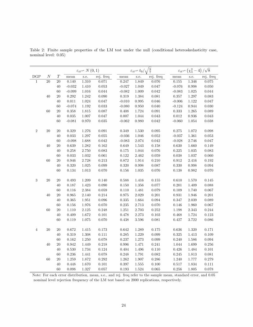
We first consider the non-bootstrap version of our test. Tables 1 and 2 report the finite sample

properties of our test under the null in the case of conditional homoskedasticity and heteroskedasticity,

respectively. We focus on the sample mean (mean), standard error (s.e.), and the rejection frequency

(rej. freq) at 0.05 nominal level for our test across 2000 simulations. Note that the asymptotic theory

suggests that has asymptotic mean 0 and standard error 1, respectively, when the null hypothesis

of slope homogeneity is satisfied. Table 1 indicates that the sample mean of tends to be positive in

finite samples, and it can be as large as 1.23 for certain DGPs; see, e.g., the case ( ) = (60 20) in

DGP 4. The is true irrespective of the distributions of the error terms. Similarly, the sample s.e. of

is generally larger than the theoretical value 1 in all DGPs for all error distributions under investigation.

In some case, the sample s.e. can be as large as 3.14 (see the case ( ) = (60 60) in DGP 2) despite the

fact that admittedly the larger sample s.e.’s tend to be driven by several outliers in the simulations and

21

if one eliminates these outliers among the 2000 replications, then s.e.’s would be significantly reduced.

In terms of rejection frequency at 0.05 nominal level, we find that 1) the test tends to be oversized,

2) the size distortion tends to increase as increases for fixed and it becomes most severe in the

case when is largest, 3) the size distortion is only mild when ≥ 1, and 4) the fat-tailedness orskewness of the error terms does not play an important role. As a referee points out, the size distortion in

the case when is large relative to is closely related to the well-known incidental parameter problem

in panel data models. The results in Table 2 for the case of conditional heteroskedasticity are largely

similar to those in Table 1. This is due to the fact that the asymptotic bias and variance formulae of our

test automatically take into account the potential presence of conditional heteroskedasticity of unknown

form.

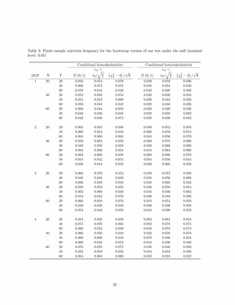
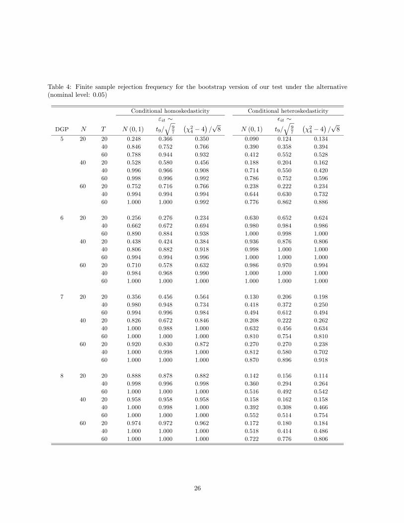
Tables 3 and 4 report the finite sample power rejection frequency of our test based on the bootstrap

-values under the null and alternative, respectively. We summarize some important findings from these

tables. First, Table 3 suggests that the level of the bootstrap version of our test tends to be well-

behaved across all DGPs under investigation. This is true regardless of the presence of conditional

heteroskedasticity or not and whether the error terms exhibit fat-tailedness or skewness or not. Second,

Table 4 suggests that the finite sample power behavior of the bootstrap version of our test is quite

satisfactory for DGPs 5-8. As either or increases, the power of our test increases, and as the

asymptotic theory predicts, it increases faster as increases for fixed than as increases for fixed

In addition, we find that the presence of conditional heteroskedasticity generally makes it harder to

detect the deviations from slope homogeneity when the signal-noise ratio is controlled.

4.2 An application to the OECD economic growth data

Economic growth model has been a key issue over many decades in macroeconomics. It is interesting

to incorporate interactive fixed effects in panel model study, which can account for heterogenous impact

of unobservable common shocks. However, the slope homogeneity assumption of Bai (2009a) can be

restrictive in empirical work. For classical panel data models there has been a number of researches

suggesting that the slope homogeneity assumption may be too restrictive in studying economic growth;

see Basssanini and Scarpetta (2002), Bond, Leblebicioglu and Schiantarelli (2010), and Eberhardt and

Teal (2011), among others. Basssanini and Scarpetta (2002) estimate a standard growth equation using

the annual data for 21 OECD countries from 1971 to 1998 and conduct the Hausman test for the long-run

slope homogeneity hypothesis. They find that the homogeneity restriction can be rejected at the 5% level

when some time dummies are added to the model. Bond, Leblebicioglu and Schiantarelli (2010) present

evidence of a positive relationship between investment as a share of gross domestic product (GDP) and

the long-run growth rate of DGP per worker and find that allowing for heterogeneity across countries in

model parameters suggests that growth rates are typically less persistent than suggested by pooled IV

22

Table 1: Finite sample properties of the LM test under the null (conditional homoskedasticity case,

nominal level: 0.05)

v (0 1) v 9q

97

v¡24 − 4

¢√8

DGP mean s.e. rej. freq mean s.e. rej. freq mean s.e. rej. freq

1 20 20 0.166 1.306 0.073 0.158 1.202 0.072 0.209 1.614 0.085

40 -0.023 1.081 0.060 -0.031 1.092 0.061 -0.021 1.044 0.055

60 -0.075 1.096 0.044 -0.077 1.013 0.041 -0.084 1.070 0.045

40 20 0.318 1.200 0.095 0.368 1.624 0.104 0.302 1.144 0.100

40 0.112 1.024 0.064 0.124 1.103 0.065 0.068 1.077 0.063

60 -0.015 1.053 0.054 -0.028 1.033 0.052 0.028 1.049 0.056

60 20 0.423 1.352 0.113 0.421 1.315 0.111 0.475 1.667 0.109

40 0.143 1.073 0.071 0.160 1.043 0.068 0.120 1.089 0.064

60 0.077 1.048 0.060 0.076 1.044 0.063 0.118 0.985 0.053

2 20 20 0.265 1.519 0.084 0.270 1.515 0.083 0.249 1.235 0.090

40 -0.035 1.242 0.055 0.006 2.024 0.052 -0.072 1.043 0.055

60 -0.111 1.331 0.046 -0.077 1.734 0.048 -0.148 1.065 0.041

40 20 0.526 1.775 0.131 0.534 1.876 0.135 0.521 1.624 0.135

40 0.065 1.025 0.062 0.082 1.098 0.066 0.128 1.782 0.067

60 0.051 1.798 0.060 0.072 2.417 0.059 -0.002 1.005 0.047

60 20 0.758 2.396 0.169 0.707 1.969 0.170 0.762 2.321 0.164

40 0.264 1.990 0.077 0.217 1.030 0.072 0.219 1.003 0.071

60 0.107 1.011 0.062 0.113 1.008 0.059 0.119 3.143 0.055

3 20 20 0.389 1.438 0.107 0.407 1.431 0.112 0.409 1.470 0.115

40 0.026 1.228 0.049 0.040 1.264 0.056 0.035 1.196 0.053

60 -0.050 2.006 0.045 -0.107 1.019 0.046 -0.072 1.606 0.044

40 20 0.718 1.735 0.166 0.800 2.148 0.167 0.770 2.091 0.168

40 0.201 1.298 0.085 0.226 1.782 0.083 0.205 1.735 0.075

60 0.052 1.094 0.054 0.043 1.001 0.059 0.133 2.477 0.065

60 20 1.021 2.134 0.246 0.995 1.981 0.235 1.049 2.704 0.225

40 0.361 1.123 0.103 0.460 2.702 0.104 0.379 2.614 0.090

60 0.304 3.263 0.070 0.186 1.533 0.064 0.265 2.699 0.071

4 20 20 0.531 1.526 0.131 0.544 1.569 0.132 0.527 1.392 0.144

40 0.091 1.688 0.066 0.081 1.503 0.066 0.125 1.706 0.065

60 -0.069 1.396 0.049 -0.036 1.793 0.044 0.032 2.380 0.053

40 20 0.909 1.787 0.215 0.922 1.809 0.217 0.891 1.608 0.210

40 0.362 2.044 0.096 0.408 2.324 0.104 0.344 2.376 0.090

60 0.114 1.560 0.064 0.202 2.554 0.070 0.216 2.935 0.074

60 20 1.226 2.019 0.294 1.231 2.064 0.296 1.237 2.394 0.285

40 0.514 2.147 0.119 0.467 1.554 0.121 0.450 2.283 0.100

60 0.324 2.923 0.079 0.251 1.957 0.076 0.238 1.311 0.080

Note: For each error distribution, mean, s.e., and rej. freq refer to the sample mean, standard error, and 0.05

nominal level rejection frequency of the LM test based on 2000 replications, respectively.

23

Table 2: Finite sample properties of the LM test under the null (conditional heteroskedasticity case,

nominal level: 0.05)

v (0 1) v 9q

97

v¡24 − 4

¢√8

DGP mean s.e. rej. freq mean s.e. rej. freq mean s.e. rej. freq

1 20 20 0.140 1.310 0.071 0.247 1.849 0.076 0.155 1.346 0.075

40 -0.032 1.410 0.053 -0.027 1.049 0.047 -0.076 0.998 0.050

60 -0.099 1.016 0.044 -0.082 1.009 0.042 -0.083 1.025 0.044

40 20 0.292 1.242 0.090 0.319 1.384 0.081 0.357 1.297 0.083

40 0.011 1.024 0.047 -0.010 0.995 0.046 -0.006 1.122 0.047

60 -0.074 1.192 0.033 -0.080 0.950 0.040 -0.124 0.944 0.030

60 20 0.358 1.815 0.087 0.408 1.724 0.091 0.333 1.265 0.089

40 0.035 1.007 0.047 0.007 1.044 0.043 0.012 0.936 0.043

60 -0.081 0.970 0.035 -0.062 0.980 0.042 -0.060 1.054 0.038

2 20 20 0.329 1.276 0.091 0.349 1.530 0.095 0.275 1.072 0.098

40 0.033 1.297 0.055 -0.036 1.046 0.052 -0.037 1.361 0.053

60 -0.098 1.688 0.042 -0.083 2.074 0.042 -0.028 2.746 0.047

40 20 0.639 1.282 0.162 0.649 1.543 0.158 0.630 1.660 0.149

40 0.258 2.750 0.083 0.175 1.044 0.076 0.225 1.035 0.083

60 0.033 1.032 0.061 0.122 2.462 0.059 0.038 1.037 0.060

60 20 0.946 2.728 0.213 0.872 1.914 0.210 0.912 2.416 0.192

40 0.320 1.025 0.099 0.320 0.998 0.087 0.330 0.998 0.094

60 0.134 1.013 0.070 0.156 1.035 0.076 0.138 0.982 0.070

3 20 20 0.493 1.209 0.140 0.588 1.416 0.155 0.610 1.570 0.145

40 0.187 1.423 0.090 0.150 1.356 0.077 0.201 1.409 0.088

60 0.116 2.384 0.059 0.110 1.481 0.079 0.109 1.740 0.067

40 20 0.965 2.140 0.214 0.975 2.029 0.201 0.931 1.946 0.201

40 0.365 1.951 0.096 0.335 1.664 0.094 0.347 2.039 0.089

60 0.156 1.976 0.070 0.235 2.713 0.070 0.146 1.960 0.067

60 20 1.110 2.125 0.248 1.251 2.703 0.252 1.198 2.343 0.244

40 0.409 1.672 0.101 0.478 2.273 0.103 0.468 1.724 0.123

60 0.119 1.075 0.070 0.438 3.596 0.081 0.427 3.722 0.086

4 20 20 0.672 1.415 0.173 0.642 1.289 0.175 0.636 1.320 0.171

40 0.319 1.308 0.111 0.285 1.229 0.099 0.325 1.413 0.109

60 0.162 1.250 0.078 0.237 1.273 0.099 0.240 1.586 0.094

40 20 0.942 1.449 0.218 0.996 1.471 0.241 1.044 1.699 0.256

40 0.530 1.734 0.124 0.404 1.496 0.110 0.426 1.484 0.101

60 0.236 1.441 0.078 0.248 1.791 0.082 0.245 1.813 0.081

60 20 1.259 1.872 0.292 1.262 1.907 0.286 1.240 1.777 0.279

40 0.448 1.670 0.101 0.397 1.555 0.100 0.517 1.834 0.111

60 0.098 1.327 0.057 0.193 1.524 0.065 0.256 1.805 0.078

Note: For each error distribution, mean, s.e., and rej. freq refer to the sample mean, standard error, and 0.05

nominal level rejection frequency of the LM test based on 2000 replications, respectively.

24

Table 3: Finite sample rejection frequency for the bootstrap version of our test under the null (nominal

level: 0.05)

Conditional homoskedasticity Conditional heteroskedasticity

∼ ∼DGP (0 1) 9

q97

¡24 − 4

¢√8 (0 1) 9

q97

¡24 − 4

¢√8

1 20 20 0.056 0.054 0.076 0.030 0.050 0.036

40 0.066 0.072 0.052 0.048 0.034 0.040

60 0.058 0.044 0.046 0.042 0.020 0.036

40 20 0.052 0.050 0.054 0.040 0.030 0.034

40 0.054 0.052 0.060 0.020 0.042 0.026

60 0.050 0.044 0.042 0.028 0.046 0.026

60 20 0.060 0.044 0.056 0.020 0.026 0.036

40 0.046 0.040 0.048 0.028 0.028 0.022

60 0.042 0.040 0.074 0.028 0.030 0.042

2 20 20 0.064 0.058 0.040 0.040 0.052 0.084

40 0.060 0.054 0.048 0.066 0.056 0.054

60 0.064 0.060 0.064 0.044 0.056 0.070

40 20 0.050 0.064 0.058 0.080 0.070 0.066

40 0.040 0.058 0.058 0.056 0.060 0.066

60 0.064 0.066 0.054 0.044 0.064 0.060

60 20 0.062 0.066 0.058 0.068 0.086 0.070

40 0.054 0.042 0.054 0.054 0.056 0.054

60 0.036 0.044 0.058 0.038 0.068 0.056

3 20 20 0.068 0.070 0.052 0.050 0.072 0.050

40 0.048 0.048 0.040 0.058 0.056 0.068

60 0.066 0.058 0.040 0.048 0.060 0.042

40 20 0.050 0.052 0.058 0.046 0.050 0.054

40 0.062 0.060 0.048 0.044 0.036 0.062

60 0.054 0.042 0.076 0.046 0.048 0.036

60 20 0.066 0.058 0.076 0.054 0.054 0.050

40 0.040 0.038 0.042 0.036 0.036 0.038

60 0.054 0.048 0.058 0.044 0.030 0.052

4 20 20 0.054 0.056 0.058 0.082 0.084 0.034

40 0.074 0.070 0.064 0.082 0.078 0.074

60 0.060 0.052 0.038 0.056 0.078 0.074

40 20 0.066 0.050 0.048 0.032 0.058 0.078

40 0.060 0.066 0.042 0.070 0.046 0.054

60 0.060 0.048 0.052 0.044 0.036 0.046

60 20 0.070 0.076 0.072 0.046 0.040 0.050

40 0.032 0.050 0.056 0.034 0.034 0.036

60 0.064 0.064 0.060 0.032 0.024 0.022

25

Table 4: Finite sample rejection frequency for the bootstrap version of our test under the alternative

(nominal level: 0.05)

Conditional homoskedasticity Conditional heteroskedasticity

∼ ∼DGP (0 1) 9

q97

¡24 − 4

¢√8 (0 1) 9

q97

¡24 − 4

¢√8

5 20 20 0.248 0.366 0.350 0.090 0.124 0.134

40 0.846 0.752 0.766 0.390 0.358 0.394

60 0.788 0.944 0.932 0.412 0.552 0.528

40 20 0.528 0.580 0.456 0.188 0.204 0.162

40 0.996 0.966 0.908 0.714 0.550 0.420

60 0.998 0.996 0.992 0.786 0.752 0.596

60 20 0.752 0.716 0.766 0.238 0.222 0.234

40 0.994 0.994 0.994 0.644 0.630 0.732

60 1.000 1.000 0.992 0.776 0.862 0.886

6 20 20 0.256 0.276 0.234 0.630 0.652 0.624

40 0.662 0.672 0.694 0.980 0.984 0.986

60 0.890 0.884 0.938 1.000 0.998 1.000

40 20 0.438 0.424 0.384 0.936 0.876 0.806

40 0.806 0.882 0.918 0.998 1.000 1.000

60 0.994 0.994 0.996 1.000 1.000 1.000

60 20 0.710 0.578 0.632 0.986 0.970 0.994

40 0.984 0.968 0.990 1.000 1.000 1.000

60 1.000 1.000 1.000 1.000 1.000 1.000

7 20 20 0.356 0.456 0.564 0.130 0.206 0.198

40 0.980 0.948 0.734 0.418 0.372 0.250

60 0.994 0.996 0.984 0.494 0.612 0.494

40 20 0.826 0.672 0.846 0.208 0.222 0.262

40 1.000 0.988 1.000 0.632 0.456 0.634

60 1.000 1.000 1.000 0.810 0.754 0.810

60 20 0.920 0.830 0.872 0.270 0.270 0.238

40 1.000 0.998 1.000 0.812 0.580 0.702

60 1.000 1.000 1.000 0.870 0.896 0.918

8 20 20 0.888 0.878 0.882 0.142 0.156 0.114

40 0.998 0.996 0.998 0.360 0.294 0.264

60 1.000 1.000 1.000 0.516 0.492 0.542

40 20 0.958 0.958 0.958 0.158 0.162 0.158

40 1.000 0.998 1.000 0.392 0.308 0.466

60 1.000 1.000 1.000 0.552 0.514 0.754

60 20 0.974 0.972 0.962 0.172 0.180 0.184

40 1.000 1.000 1.000 0.518 0.414 0.486

60 1.000 1.000 1.000 0.722 0.776 0.806

26

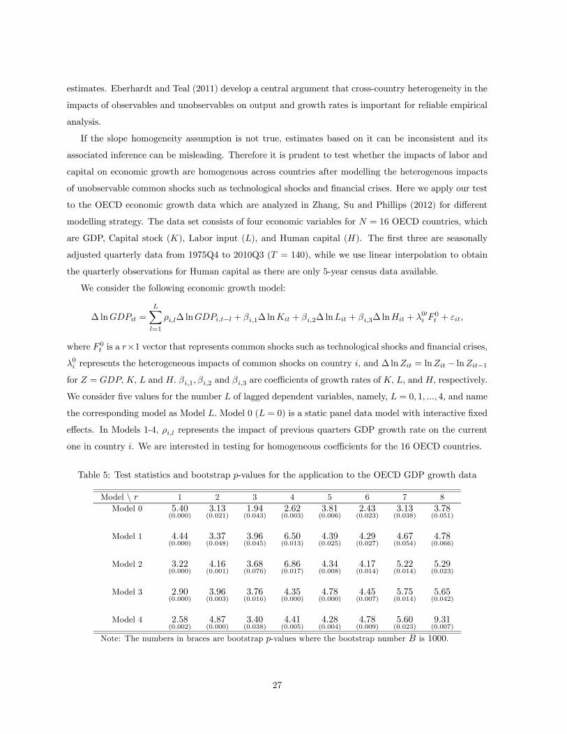
estimates. Eberhardt and Teal (2011) develop a central argument that cross-country heterogeneity in the

impacts of observables and unobservables on output and growth rates is important for reliable empirical

analysis.

If the slope homogeneity assumption is not true, estimates based on it can be inconsistent and its

associated inference can be misleading. Therefore it is prudent to test whether the impacts of labor and

capital on economic growth are homogenous across countries after modelling the heterogenous impacts

of unobservable common shocks such as technological shocks and financial crises. Here we apply our test

to the OECD economic growth data which are analyzed in Zhang, Su and Phillips (2012) for different

modelling strategy. The data set consists of four economic variables for = 16 OECD countries, which

are GDP, Capital stock (), Labor input (), and Human capital (). The first three are seasonally

adjusted quarterly data from 1975Q4 to 2010Q3 ( = 140) while we use linear interpolation to obtain

the quarterly observations for Human capital as there are only 5-year census data available.

We consider the following economic growth model:

∆ ln =

X=1

∆ ln− + 1∆ ln + 2∆ ln + 3∆ ln + 00 0 +

where 0 is a ×1 vector that represents common shocks such as technological shocks and financial crises,0 represents the heterogeneous impacts of common shocks on country , and ∆ ln = ln − ln−1for = and 1 2 and 3 are coefficients of growth rates of and respectively.

We consider five values for the number of lagged dependent variables, namely, = 0 1 4 and name

the corresponding model as Model Model 0 ( = 0) is a static panel data model with interactive fixed

effects. In Models 1-4, represents the impact of previous quarters GDP growth rate on the current

one in country . We are interested in testing for homogeneous coefficients for the 16 OECD countries.

Table 5: Test statistics and bootstrap -values for the application to the OECD GDP growth data

Model \ 1 2 3 4 5 6 7 8

Model 0 540(0000)

313(0021)

194(0043)

262(0003)

381(0006)

243(0023)

313(0038)

378(0051)

Model 1 444(0000)

337(0048)

396(0045)

650(0013)

439(0025)

429(0027)

467(0054)

478(0066)

Model 2 322(0000)

416(0001)

368(0076)

686(0017)

434(0008)

417(0014)

522(0014)

529(0023)

Model 3 290(0000)

396(0003)

376(0016)

435(0000)

478(0000)

445(0007)

575(0014)

565(0042)

Model 4 258(0002)

487(0000)

340(0038)

441(0005)

428(0004)

478(0009)

560(0023)

931(0007)

Note: The numbers in braces are bootstrap -values where the bootstrap number is 1000.

27

We consider = 1 2 8 to capture the interactive fixed effects in the growth model.8 Table 5

reports the test statistics and the bootstrap -values for our test of slope homogeneity. From the table,

we see that the bootstrap -values for all numbers of factors under investigation are uniformly much

smaller than 010 in all cases and smaller than 0.05 in most cases. So we can reject the null hypothesis

of homogeneous slopes at the 5% level for all models for a majority of values of . The results imply that

the slope homogeneity assumption may not be plausible at all despite the fact it is commonly assumed

in the literature (c.f., Eberhardt and Teal (2011, p. 109)). So it implies we have to resort to Pesaran’s

(2006) CCE method to obtain the heterogenous impacts of labor and capital on economic growth across

OECD countries.

5 Conclusions

In this paper we propose an LM test for slope homogeneity in large dimensional dynamic panel data models

with interactive fixed effects and conditional heteroskedasticity of unknown form. We first estimate the

model under the null to obtain the restricted residuals which are then used to construct the test statistic.

We demonstrate that after being appropriately normalized, it is asymptotically normally distributed

under the null hypothesis of homogeneous slopes and it has power to detect Pitman local alternatives

at the rate of −12−14 We also propose a wild bootstrap procedure to obtain the bootstrap -

values. Simulations demonstrate that the bootstrap version of our test behaves reasonably well in finite

samples. The application to the OECD economic growth data indicates that the commonly imposed

slope homogeneity assumption is rather fragile.

When the null hypothesis of homogeneous slopes is rejected, we may consider applying Pesaran’s

(2006) CCE method to obtain consistent estimates of both individual slopes and their cross-sectional

average under certain rank conditions. If some prior information is available, one can divide the cross

sectional units into several groups, test the slope homogeneity within each group, and estimate the

homogenous slopes within each individual group in the case of failure of rejection. Alternatively, a panel

structure model in the spirit of Sun (2005) may be considered.

Notes

1The rank condition must also be satisfied when estimating the homogenous model.

2Under the standard assumption that () = 0 for each also centers around 0 for each under

the null in the sense = + (1) so that an intercept term in the above regression is unnecessary.

3For an excellent survey on LM-principle-based misspecification tests, see Godfrey (1988).

4Alternatively, cross-sectional dependence can be generated via the specification of spatial weight

28

matrix, which is regularly used in the spatial econometrics literature; see, e.g., Anselin (1988). But this

type of cross-sectional dependence is local in nature.

5Let ≡ (1 )0 Noting that 0 = we have =Ω−12

6An alternative expression for is given by

≡

¡ 0¢=

1

X=1

0 0 − 1

Ã1

2

X=1

X=1

0 0

!=

1

X=1

0

which is used by Bai (2009a).

7This is the case even if contains lagged dependent variables, say, −1 and −28Alternatively, one can use the information criteria proposed by Bai and Ng (2002) to determine the

number of factors. But it is well known that their criteria tend to fail when the cross sectional unit

is small, which is the case here.

REFERENCES

Andrews, D. W. K. (2005) Cross-section regression with common shocks. Econometrica 73, 1551-1585.

Anselin, L. (1988) Spatial Econometric Methods and Models. Kluwer, Boston.

Bai, J. (2009a) Panel data models with interactive fixed effects. Econometrica 77, 1229-1279.

Bai, J. (2009b) Supplement to “Panel data models with interactive fixed effects”: technical details and

proofs. Econometrica Supplementary Material.

Bai, J. & S. Ng (2002) Determining the number of factors in approximate factor models. Econometrica

70, 191-221.

Bai, J. & S. Ng (2006) Evaluating latent and observed factors in macroeconomics and finance. Journal

of Econometrics 131, 507-537.

Baltagi, B. H., G. Bresson, & A. Pirotte (2008) To pool or not to pool? In L. Mátyás and P. Sevestre

(eds.), The Econometrics of Panel Data, pp. 517-546, Springer-Verlag, Berlin.

Bassanini, A. & S. Scarpetta (2002) Does human capital matter for growth in OECD countries? A

pooled mean-group approach. Economics Letter 74, 399-405.

Bernstein, D. S. (2005) Matrix Mathematics: Theory, Facts, and Formulas with Application to Linear

Systems Theory. Princeton University Press, Princeton.

Blomquist, J. (2010) A panel bootstrap test for slope homogeneity. Working paper, Lund University.

Bond, S., A. Leblebicioglu & F. Schiantarelli (2010). Capital accumulation and growth: a new look at

the empirical evidence. Journal of Applied Econometrics 25, 1073-1099.

29

Connor, G. & R. Korajzcyk (1998) Risk and return in an equilibrium APT application of a new test

methodology. Journal of Financial Economics 21, 225-289.

Eberhardt, M. & F. Teal (2011) Econometrics for grumblers: a new look at the literature on cross-

country growth empirics. Journal of Economic Surveys 25, 109-155.

Fama, E., K. & K. French (1993) Common risk factors in the returns on stocks and bonds. Journal of

Financial Economics 18, 61-90.

Godfrey, L. G. (1988) Misspecification Tests in Econometrics: The Lagrangian Multiplier Principle and

Other Approaches. Cambridge University Press, Cambridge.

Gonçalves, S. & L. Kilian (2004). Bootstrapping autoregressions with conditional heteroskedasticity of

unknown form. Journal of Econometrics 123, 89-120.

Greenaway-McGrevy, R., C. Han, & D. Sul (2012) Asymptotic distribution of factor augmented estima-

tors for panel regression. Journal of Econometrics 169, 48-53.

Hahn, J. & G. Kuersteiner (2011) Reduction for dynamic nonlinear panel models with fixed effects.

Econometric Theory 27, 1152-1191.

Hansen, B. E. (2000) Testing for structural change in conditional models. Journal of Econometrics 97,

93-115.

Hsiao, C. (2003) Analysis of Panel Data. Cambridge University Press, Cambridge.

Jin, S. & L. Su (2013) A nonparametric poolability test for panel data models with cross section depen-

dence. Econometric Reviews 32, 469-512.

Kapetanios, G. & M. H. Pesaran (2007) Alternative approaches to estimation and inference in large

multifactor panels: small sample results with an application to modelling of asset return. In G.

Phillips and E. Tzavalis (eds.), The Refinement of Econometric Estimation and Testing Procedures:

Finite Sample and Asymptotic Analysis, Cambridge University Press, Cambridge.

Lee, A. J. (1990) U-statistics: Theory and Practice. Marcel Dekker, New York.

Lehmann, B. & D. Modest (1988) The empirical foundations of the arbitrage pricing theory. Journal of

Financial Economics 21, 213-254.

Lin, C-C. (2010) Testing for slope homogeneity in a linear panel model with fixed effects and conditional

heteroskedasticity. Working paper, Institute of Economics, Academia Sinica.

30

Moon, H. & M. Weidner (2010a) Linear regression for panel with unknown number of factors as inter-

active fixed effects. Working paper, University of Southern California.

Moon, H. & M. Weidner (2010b) Dynamic linear panel regression models with interactive fixed effects.

Manuscript. Working paper, University of Southern California.

Pesaran, M. H. (2006) Estimation and inference in large heterogeneous panels with a multifactor error

structure. Econometrica 74, 967-1012.

Pesaran, H., R. Smith, & K. S. Im (1996) Dynamic linear models for heterogeneous panels. In: L.

Mátyás and P. Sevestre (Eds.), The Econometrics of Panel Data: A Handbook of the Theory with

Applications, second revised edition, pp.145—195, Kluwer Academic Publishers, Dordrecht.

Pesaran, M. H. & T. Yamagata (2008) Testing slope homogeneity in large panels. Journal of Econo-

metrics 142, 50-93.

Pesaran, M. H. & E. Tosetti (2011) Large panels with common factors and spatial correlation. Journal

of Econometrics 161, 182-202.

Phillips, P. C. B. & D. Sul (2003) Dynamic panel estimation and homogeneity testing under cross section

dependence. Econometrics Journal 6, 217—259.

Pollard, D. (1984) Convergence of Stochastic Processes. Springer-Verlag, New York.

Prakasa Rao, B. L. S. (2009) Conditional independence, conditional mixing and conditional association.

Annals of the Institute of Statistical Mathematics 61, 441-460.

Roussas, G. G. (2008) On conditional independence, mixing and association. Stochastic Analysis and

Applications 26, 1274-1309.

Su, L. & S. Jin (2012) Sieve estimation of panel data models with cross section dependence. Journal of

Econometrics 169, 34-47.

Su, L. & A. Ullah (2013) A nonparametric goodness-of-fit-based test for conditional heteroskedasticity.

Forthcoming in Econometric Theory.

Sun, Y. (2005) Estimation and inference in panel structure models. Working paper, Department of

Economics, UCSD.

Zhang, Y., L. Su, & P. C. B. Phillips (2012) Testing for common trends in semiparametric panel data

models with fixed effects. Econometrics Journal 15, 56-100.

31

APPENDIX

In this appendix we first provide some technical lemmas and then use them to prove the main results in

the paper. The proof of these lemmas and Theorem 3.2 are provided online at Cambridge Journals Online

in supplementary material to this article. Readers may refer to the supplementary material associated

with this article, available at Cambridge Journals Online (journals.cambridge.org/ect).

A Some Technical Lemmas

To proceed, we first provide the definition for conditional strong mixing processes, and then proceed to

prove some technical lemmas that are used in the proof of the main results in the paper.

Definition A.1 Let (ΩA ) be a probability space and B be a sub--algebra of A. Let B (·) ≡ (·|B) Let ≥ 1 be a sequence of random variables defined on (ΩA ) The sequence ≥ 1 is saidto be conditionally strong mixing given B (or B-strong-mixing) if there exists a nonnegative B-measurablerandom variable B () converging to 0 a.s. as →∞ such that

|B ( ∩)− B ()B ()| ≤ B () a.s. (A.1)

for all ∈ (1 ) ∈ ¡+ ++1

¢and ≥ 1 ≥ 1

The above definition is due to Prakasa Rao (2009); see also Roussas (2008). When one takes B () as

the supremum of the left hand side object in (A.1) over the set ∈ (1 ) ∈ ¡+ ++1

¢

≥ 1 we refer it to the B-strong-mixing coefficient.Let signify a generic constant whose exact value may vary from case to case. Let D denote an

(1) object that depends on D ≡© 0 0

ª Let ≡ min(

√√ ) and ≡ −14−12 Let

D (·) ≡ (·|D). Let D (·) and VarD (·) denote the conditional expectation and variance given D, respec-tively. Let kkD ≡ [D(kk)]1 Let ≡ 00

¡000

¢−10 and ≡ 00

¡ 00 0

¢−1 0 Let

Φ1 ≡ 0¡000

¢−1 ¡ 00 0

¢−1 00 Φ2 ≡ 0

¡ 00 0

¢−1 ¡000

¢−1 ¡ 00 0

¢−1 00, and Φ3 ≡ 0

¡000

¢−1¡ 00 0

¢−1 ¡000

¢−100

Let ≡ − 0β

0− 00 0 ≡ (1 · · · )0 and e ≡ (1 )0 Note that = +0

under H1 ( ) Let (1)

and (2)

denote × 1 vectors whose ’th elements are respectively given by

(1)

=1

tr (0X 0e0) and (A.2)

(2)

= − 1

tr (e 0e00XΦ01 + e

00e0 0XΦ1 + e

00X 0e0Φ1) (A.3)

The following lemma studies the asymptotic property of β under H1 ( )

Lemma A.2 Suppose Assumptions A.1-A.3 hold. Then under H1 ( )

β − β0 = −1 (

(1)

+ (2)

) + £2

¡−1 +

¢+

−3

¤1232

Remark. Noting that under H1 ( ) with = −14−12 (1) =1tr(0X 0∆0) +

1

tr(0X 0ε0) = ( )−1tr(0X 0∆0) +

¡[( )−12 + −1]−1

¢= (1) and sim-

ilarly (2)

=

¡−1−1 +

¢= (1) we have

β − β0 = −1Π + ( ) under Assumption A.3 (A.4)

where Π is defined in (3.7). This means that (2)

and the second term in (1)

are asymptotically

smaller than the first term in (1)

so the convergence rate of β mainly hinges on the rate of local

alternatives that converge to the null.

Let ≥ 1 be an -dimensional conditional strong mixing process with mixing coefficient D (·)and distribution function (·|D) given D The following lemma extends Davydov’s inequality from the

unconditional version to a conditional version.

Lemma A.3 Suppose that 1 and 2 are random variables which are measurable with respect to (1 )

and ¡+

¢ respectively, and that k1kD and k2kD are bounded in probability, where 1

and −1 + −1 1 Then |D (12)−D (1)D (2)| ≤ 8 k1kD k2kD D ()1−−1−−1

The following lemma extends the Bernstein-type inequality for unconditional strong mixing processes

to that for conditional strong mixing processes.

Lemma A.4 Suppose that the conditional strong mixing process ≥ 1 has zero mean given D,sup≥1 || ≤0 and sup≥1 |VarD ()| ≤D Then for any 0 and ≤

D

ï¯−1

X=1

¯¯ ≥

!≤ 2 exp

µ− 2

4D + 203

¶+ 2D ()

Define theth order U-statistic U =⎛⎝

⎞⎠−1P1≤1≤

¡1

¢where is symmetric

in its arguments. Let (0) =R · · · R (1 )Π=1 ( |D) and () (1 ) = R · · · R (1

+1 ) Π=+1 ( |D) for = 1 Let (1) () = (1) () − (0) and () (1 ) =

() (1 )−P−1

=1

P()

()¡1

¢−(0) for = 2 where the sumP

() is taken over all

subsets 1 ≤ 1 2 · · · ≤ of 1 2 Let H()

=

⎛⎝

⎞⎠−1 P1≤1≤ ()

¡1

¢

Then by Theorem 1 in Lee (1990, p. 26), we have the following Hoeffding decomposition

U = (0) +

X=1

⎛⎝

⎞⎠H()

(A.5)

To study the second moment of H()

for 3 ≤ ≤ we need the following lemma.

33

Lemma A.5 Let ≥ 1 be an -dimensional strong mixing process conditional on D with mixing

coefficient D (·) and distribution function (·|D) Let the integers (1 ) be such that 1 ≤ 1 2

· · · ≤ Suppose that maxR | (1 )|1+ 1 (1 |D)

R | (1 )|1+ 1 (1 |D) +1 (+1 |D) ≤ D(1 ) for some 0 , where, e.g., 1 (1 |D)denotes the distribution function of

¡1

¢given D. Then¯Z

(1 ) 1 (1 |D)−Z

(1 ) (1)1

(1 |D) +1 (+1 )¯

≤ 4D (1 )1(1+)

D (+1 − )(1+)

Lemma A.6 Let ≥ 1 be an -dimensional strong mixing process conditional on D with mixing

coefficient D (·) and distribution function (·|D) Suppose that D () =

¡−3(2+)−

¢ If there

exists 0 such that

≡ max½Z

| (1 · · · )|2+ Π=1 ( |D) D¯¡1

¢¯2+¾ ≤ X=1

D ()

and −1P

=1

P=1

D () = (1) then D[H()

]2 =

¡−3

¢for 3 ≤ ≤

Lemma A.7 Recall Ω ≡ D ( 0) and Ω ≡ 0

Suppose Assumptions A.1-A.3 hold. Then

() 1(Ω) ≤ 1 (Ω)+

¡−12

¢ () min(Ω) ≥ min (Ω)−

¡−12

¢ () max1≤≤ ||Ω−Ω|| =

( ) and ()max1≤≤ ||Ω−1 −Ω−1 || = ( ) where ≡ max( )1(4+2)

log ( )

(log ( ) )12

Lemma A.8 Recall ≡ 0 0 and denotes the ( )’th element of : =

P=1

P=1

0 (

0)

−1 where denotes the ( )’th element of 0 Let ≡ −1

P=1

P=1

0

Ω−1 Suppose Assumptions A.1-A.3 hold. Then 1 ≡ −12P

=1

P1≤6=≤

¡ −

¢= (1)

Lemma A.9 Suppose Assumptions A.1-A.3 hold. Then

() 21 ≡ −2−12P

=1

P1≤≤

P=1 [ −D ()]

0Ω−1 = (1)

() 22 ≡ −3−12P

=1

P1≤≤

P=1

P=1 [ −D ()]

0Ω−1 [ −D ()]

× = (1)

() 23 ≡ −3−12P

=1

P1≤≤

P=1

P=1 [ − D ()]

0Ω−1 D () =

(1)

Lemma A.10 Suppose Assumptions A.1-A.3 hold. Then 3 ≡ −12P

=1 0 0

0

= (1)

B Proof of the Results in Section 3

Proof of Theorem 3.1. The proof is a special case of that of Theorem 3.3 and thus omitted. ¥

34

Proof of Theorem 3.2. The theorem can be proved under H1 ( ) The proof is quite involved and

given in the supplementary appendix. ¥

Proof of Theorem 3.3. Following Moon and Weidner (2010a), we can readily show that

= 0 +

X=1

³0 −

´

(0)

+ (1) + (2) + () (B.1)

where

(0)

= − 0X0Φ1 − Φ01X 0 for = 1

(1) = − 0ε0Φ1 −Φ01ε 0

(2) = 0ε0Φ1ε0Φ1 + Φ01εΦ01ε 0 − 0ε00εΦ2 −Φ2ε00ε 0 − 0ε0Φ3ε 0 +Φ01ε 0ε0Φ1

and the remainder () satisfies°°° ()°°°

=

µ³−1 + +

°°°β − β0°°°´°°°β − β0°°°+ ( )−32

max³√

ë3+ 3

¶=

¡−1 + −3

¢=

¡−1

¢under Assumption A.3 () . (B.2)

It is straightforward to show that°°° (0)

°°°= (1) for = 1

°°° (1)°°°= (

−12) and°°° (2)

°°°=

¡−2

¢ (B.3)

Combining (B.1) with (2.12) yields

=

" 0 ( + ) +

X=1

³0 −

´

(0)

¡ + 00 +

¢#+ (1)

¡ + 00 +

¢+³ (2) + ()

´ ¡ + 00 +

¢≡ 1 + 2 + 3 say, (B.4)

where ≡ (β0 − β) +

¡β0 − β0

¢= (β

0 − β) + satisfies

kk = ( ) kk (B.5)

It follows thatp = −12

X=1

(1 + 2 + 3)0

(1 + 2 + 3)−

=

(−12

X=1

011 −

)+−12

X=1

022 +−12

X=1

033

+2−12X=1

012 + 2

−12X=1

013 + 2

−12X=1

023

≡ (1 − ) +2 +3 + 24 + 25 + 26 , say.

35

We complete the proof by showing that under H1( ), () 1 − − Θ→ (0 0) ()

= (1) for = 2 6, where Θ is defined in (3.9). We prove () in Proposition B.1 and () in

Propositions B.2-B.6 below.

Proposition B.1 1 − −Θ→ (0 0) under H1 ( )

Proof. Observe that 1 = −12P

=1 01

1 = 11 +12 + 213 where

11 = −12X=1

(0 + 0) 0 0 ( + )

12 = −12X=1

X=1

³0 −

´¡0 + 00

00 + 0¢

(0)

X=1

³0 −

´

(0)

¡ + 00 +

¢

13 = −12X=1

(0 + 0) 0

X=1

³0 −

´

(0)

¡ + 00 +

¢

We prove the proposition by showing that () 11− −Θ1→ (0 0) () 12 = Θ2 +

(1) and () 13 = Θ3 + (1) where

Θ1 ≡ ( )−1

X=1

¡ −−1Π

¢0 0 0

0( −−1Π )

Θ2 ≡ ( )−1

X=1

¡−1Π

¢0 0

¡−1Π

¢

Θ3 ≡ ( )−1

X=1

¡ −−1Π

¢0 0 0

¡−1Π

¢

and ≡ −1P

=1 0 The result follows because in view of the fact that 0− 0−1

×Π+−1Π = 0−( 0−−1

P=1 0)

−1Π = 0−

−1Π

we have Θ1 +Θ2 +2Θ3 = ( )−1P

=1( 0−−1Π )

0( 0−

−1Π )

= Θ

Step 1. We prove () 11 − −Θ1→ (0 0) under H1 ( ) Observe that

11 − −Θ1 =

Ã−12

X=1

0 0 0 −

!

+

Ã−12

X=1

0 0 0 −Θ1

!+ 2−12

X=1

0 0 0

≡ 111 +112 + 2113 say.

It suffices to show that: (1) 111→ (0 0) (2) 112 = (1) and (3) 113 = (1)

First, we show (1) Recall = 0 0 denotes the ( )’th element of : =P

=1

P=1

0 (

0)

−1 and ≡ −1

P=1

P=1

0Ω−1 Then we have

111 =2√

X=1

X1≤≤

+2√

X=1

X1≤≤

¡ −

¢ ≡ 1111+1112 say.

36

By Lemma A.8, 1112 = (1) Using = 1 − −1 we have

1111 =2

√

X=1

X1≤≤

X=1

X=1

0Ω−1

=2

√

X=1

X1≤≤

0Ω−1

− 4

2√

X=1

X1≤≤

X=1

D ( 0)Ω

−1

+2

3√

X=1

X1≤≤

X=1

X=1

D ( 0)Ω

−1 D ()

− 4

2√

X=1

X1≤≤

X=1

[ −D ()]0Ω−1

+2

3√

X=1

X1≤≤

X=1

X=1

[ −D ()]0Ω−1 [ −D ()]

+4

3√

X=1

X1≤≤

X=1

X=1

[ −D ()]0Ω−1 D ()

≡ 1111 +1111 +1111 +1111 +1111 +1111 say.

By Lemma A.9, 1111+1111+1111 = (1) We are left to show that ≡ 1111

+1111 +1111→ (0 0) Observe that

=2

√

X=1

X1≤≤

à − −1

X=1

D ()

!0Ω−1

à − −1

X=1

D ()

!

=

X=2

where ≡ 2−1−12P

=1

P−1=1

0 ≡ Ω−12 and ≡ −−1

P=1 D ()

By Assumptions A.2()

(|F−1) ≡ 2−1−12X=1

−1X=1

0(|F−1) = 0

That is, F is an m.d.s. By the martingale CLT [e.g., Pollard (1984, p. 171)], it suffices to

show that:

Z ≡X=2

F−1 ||4 = (1) and

X=2

2 − = (1) (B.6)

where F−1 denotes expectation conditional on F−1Observing that Z ≥ 0 it suffices to show Z = (1) by showing that D (Z) = (1) by Markov’s inequality. Noting that () are independent

37

across given D by Assumption A.2(), and F is an m.d.s. by Assumption A.2(), we have

D (Z) =16

42

X=2

X=1

X=1

X=1

X=1

X1≤≤−1

D¡0

0

0

0

¢= 48Z1 + 16Z2

where

Z1 ≡ 1

42

X=2

X=1

X=1 6=

X1≤≤−1

D¡0

0

2

¢D

¡0

0

2

¢ (B.7)

Z2 ≡ 1

42

X=2

X=1

X1≤≤−1

D¡0

0

0

0

4

¢ (B.8)

For the moment we assume that = 1 so that we can treat the ×1 vector as a scalar. [The generalcase follows from the Slutsky lemma and the fact that 0

0 =

P=1

P=1 where

denotes the ’th element of ] To bound the summation in (B.7), we consider three cases for the

time indices in ≡ − 1 : () # = 5 () # = 4 and () # ≤ 3 We use 1 1 and1 to denote the corresponding summations when the time indices are restricted to be cases (), ()

and () respectively. In case () using Davydov’s inequality in Lemma A.3 yields

¯D

¡

2

¢¯ ≤ 89D ( )D (− 1− ( ∨ ))(1+)(2+) (B.9)

where ∨ ≡ max ( ) and 9D ( ) ≡°°°°4+2D °°22°°4+2D Similar inequality holds

for D( 2) By the repeated use of Cauchy-Schwarz’s and Jensen’s inequalities,

|9D (1 2 3)| ≤ 1

2

h°°2 323°°24+2D + °°2121°°24+2Di≤ 1

4

n°°°°28+4D + °°33°°28+4D + 2°°2121°°24+2Do ≤ 3X=1

9D ()

where 9D () = 12°°°°28+4D + °°22°°24+2D With this, we can readily show that

1 ≤

4

X1=2

⎧⎨⎩ 1

X=1

X1≤23≤1−1

"3X

=1

9D ()

#D (1 − 1− (2 ∨ 3))(1+)(2+)

⎫⎬⎭2

=

¡−1

¢

In case () we consider two subcases: (1) one and only one of equals −1 (2) # = 3We use 11 and 12 to denote the corresponding summations when the individual indices are

restricted to subcases (1) and (2) respectively. In subcase (1) wlog we assume that = − 1 andapply that ¯

D¡ −1−12

¢¯ ≤ 810D ( )D (− 1− )(1+)(2+)

for 10D ( ) ≡°°°°8+4D °°2−1−12°°(8+4)3D ≤ 10D () + 10D () with 10D () ≡

38

°°°°28+4D + °°2−1−12°°2(8+4)3D and (B.9) to obtain11 ≤

4

X1=2

⎧⎨⎩ 1

X=1

X1≤23≤1−1

"3X

=1

9D ()

#D (1 − 1− (2 ∨ 3))(1+)(2+)

⎫⎬⎭×⎧⎨⎩ 1

X=1

X1≤4≤1−1

£10D (1) + 10D (4)

¤D (1 − 1− 4)

(1+)(2+)

⎫⎬⎭=

¡−1

¢

In subcase (2) wlog we assume that = and −1We consider two subsubcases: (21) either− 1− ∗ or − ∗, (22) − 1− ≤ ∗ and − ≤ ∗ In the first case, we have

¯D

¡

2

¢¯ ≤⎧⎨⎩ 811D ( )D (∗)

(1+)(2+)if − 1− ∗

812D ( )D (∗)(1+)(2+)

if − ∗

where 11D ( ) ≡°°2°°4+2D °°°°4+2D and 12D ( ) ≡ °°2°°(8+4)3D°°°°8+4D These results, in conjunction with the fact that the total number of terms in the sum-

mation in subcases (22) is of order ¡2 32∗

¢ imply that

12 ≤

³ 2D (∗)

(1+)(2+)´+ −4−2

¡2 32∗

¢=

³ 2D (∗)

(1+)(2+)+ −12∗

´= (1) by Assumption A.2 ()

Consequently, 1 = (1) In case () we have 1 =

¡−1

¢as the number of terms in the

summation is ¡2 3

¢and each term in absolute value has bounded expectation. It follows that

Z1 = (1)

To bound Z2 we consider two cases for the set of indices ≡ − 1, () # = 5, and ()all the other cases. We use 2 and 2 to denote the corresponding summations when the individual

indices are restricted to subcases () and () respectively. In the first case, letting = max( ) we

have ¯D

¡4

4

¢¯ ≤ 813D ( )D (− 1− )(2+)

where 13D ( ) ≡°° °°2+D °°44°°2+D It is easy to verify that13D(1 2

3 4 5) ≤P5

=1 13D ()where 13D () ≡°°°°28+4D Then2 ≤ −2−1

P=1

P=1 13D ()P

=1 D ()(2+)

=

¡−1

¢ In case () we have 2 =

¡−1

¢ It follows that Z2 =

¡−1

¢and thus Z = (1) Consequently the first part of (B.6) follows.

For the second part of (B.6), noting that () are independent across given D by Assumption

A.2(), and F is an m.d.s. by Assumption A.2(), we have by the law of iterated expectations

39

that

X=2

D(2) = 4−2−1X=2

D

"X=1

−1X=1

0

#2

= 4−2−1X=2

X=1

−1X=1

−1X=1

D(2 0

0) =

In addition, we can show by straightforward moment calculations that D(P

=2 2)

2 = 2 + (1)

Thus VarD(P

=2 2) = (1) and the second part of (B.6) follows.

Next we show (2) Let ≡

¡ −−1Π

¢ Then by (A.4)

=

¡ −−1Π

¢+ ( ) = + ( ) (B.10)

Noting that−12P

=1 0 0

0 = ( )−1P

=1

¡ −−1Π

¢ 0 0

0( −−1

Π ) = Θ1 we have

112 = −12X=1

( − )0 0

0 ( − ) + 2−12

X=1

0 0 0 ( − )

≡ 1121 + 21122 say.

By (B.10), the fact thatP

=1 kk2 = ( ), k 0k = 1 and kk = 1

|1121| ≤ −12X=1

k − k2 = (2 )

−12X=1

kk2 = (2 )

³12

´= (1)

Similarly, we can show that 1122 = (1) This completes the proof of (2)

Now we show (3) We decompose 113 as follows

113 = −12

X=1

0 0 0 +−12

X=1

0 0 0(β

0 − β)

≡ 1131 +1132(β0 − β) say.

In view of the fact that ||β0 − β|| = ( ) we can prove 113 = (1) by showing that (3)

1131 = (1) and (3) 1132 = (1) (3) is proved in Lemma A.10 and (3) can be

proved analogously, say by taking as a × 1 vector of ones. This completes the proof of (3).

Step 2. We prove () 12 = Θ2 + (1) under H1 ( ) First, we decompose 12 as

follows

12 =

X=1

³0 −

´ X=1

³0 −

´−12

X=1

00 00 (0)

(0)

00

+

X=1

³0 −

´ X=1

³0 −

´−12

X=1

0 (0)

(0)

+ 0(0)

(0)

+ 20(0)

(0)

00 + 20

(0)

(0)

+ 20

00 (0)

(0)

≡ 121 +122 say.

40

We want to show that (1) 121 = Θ2 + (1) and (2) 12 = (1) (1) follows because

121 = −12X=1

³0 −

´ X=1

³0 −

´ X=1

00 00Φ01X 0

0X0Φ1

00

= −12X=1

³0 −

´ X=1

³0 −

´ X=1

00¡000

¢−100X 0

0X00¡000

¢−10

=1

X=1

0−1Π

X=1

0−1Π

X=1

00¡000

¢−100X 0

0X00¡000

¢−10

+ (1)

=1

X=1

X=1

0−1Π

0·

X=1

0−1Π · + (1)

=1

X=1

¡−1Π

¢0 0

¡−1Π

¢+ (1) = Θ2 + (1)

where is a × 1 vector with 1 in the th place and zeros elsewhere, and ≡ −1P

=1 0

is a × matrix whose th column is given by · ≡³00¡000

¢−100X 0

´0

To show (2) we assume that = 1 for notational simplicity. We write X andP

=1(0− ) (0)

simply as X and (β0 − β) (0) respectively, where (0) = − 0X0Φ1 −Φ01X 0 Then

122 =³β0 − β

´2−12

X=1

0 (0) (0) + 0

(0) (0) + 2

0

(0) (0) 00

+ 20(0)

(0) + 20

00 (0) (0)

≡³β0 − β

´21221 +1222 + 21223 + 21224 + 21225 say.

Noting that ||β0− β|| = ( ) it suffices to prove (2) by showing that 122 ≡ 2122 =

(1) for = 1 2 5 Noting that kk = 1 and°°° (0)

°°° = k( 0X0Φ1 +Φ01X 0) k =

³−12

´°° 00°°+

³−12−12

´kX0k (B.11)

and by (B.3) and (B.10), we have

¯1221

¯≤ 2

−12X=1

°°° (0)

°°°2 ≤ 2

X=1

h

³−12

´°° 00°°+

³−12−12

´kX0k

i2=

¡−1−1

¢ () =

¡−1

¢= (1) ¯

1222

¯≤

¡2

¢( )

−1°°° (0)

°°°2 X=1

kk2 =

¡2

¢( )

−1 ( ) =

¡2

¢= (1)

¯1223

¯≤ 2

−12X=1

°°° (0)

°°°°°° (0) 00

°°°≤ ( )

−1°°° (0) 0

°°° X=1

h

³−12

´°° 00°°+

³−12−12

´kX0k

i °°0°°= ( )

−1

³ 12

´ () =

³−12

´= (1)

41

¯1224

¯≤ 2

−12X=1

°°° (0)

°°°°°° (0)

°°°≤ ( ) ( )

−1°°° (0)

°°° X=1

h

³−12

´°° 00°°+

³−12−12

´kX0k

ikk

= ( )−1

³ 12

´=

³−12

´= (1)

and¯1225

¯≤ ( )

−1 °° (0)°°2P

=1

°° 00°° kk = ( )−1

( ) = (1)

Step 3. We prove () 13 = Θ3 + (1) under H1 ( ) First, we decompose 13 as

follows

13 =

X=1

³0 −

´−12

X=1

0 0

(0)

00

+

X=1

³0 −

´−12

X=1

(0 + 0) 0

(0)

( + ) + 0 0

(0)

00

≡ 131 +132 say.

We prove () by showing that (1) 131 = Θ3 + (1) and (2) 132 = (1) (1)

follows because by (A.4)

131 = −−12X=1

³0 −

´ X=1

0 0 0X0

Φ100

= −−12X=1

³0 −

´ X=1

0 0 0X0

0¡000

¢−10

=1

X=1

0−1Π

X=1

¡ −−1Π

¢0 0 0

0X0

0¡000

¢−10 + (1)

=1

X=1

¡ −−1Π

¢0 0 0

X=1

0−1Π · + (1)

=1

X=1

¡ −−1Π

¢0 0 0

¡−1Π

¢+ (1) = Θ3 + (1)

To show (2) again we assume that = 1 for notational simplicity. As before, we write X andP=1(

0 − )

(0)

simply as X and (β0−β) (0) respectively. Then

132 =³β0−β

´−12

X=1

0 0 (0) + 0 0

(0) + 0 0 (0)

+ 0 0 (0) + 0 0

(0) 00 ≡

³β0−β

´(1321 +1322 +1323 +1324 +1325) say.

We prove (2) by showing that 132 ≡ 132 = (1) for = 1 2 5

42

For 1321 note that 1321 = −12P

=1 0

(0)−−12P

=1 0 0

(0) ≡1321 − 1321 say.

¯1321

¯=

¯¯trà (0)−12

X=1

0

!¯¯ ≤

°°° (0)°°°

¯¯trÃ−12

X=1

0

0 (

0)

−1!¯¯

≤

°°° (0)°°°

∙min1≤≤

min (0 )

¸−1tr

Ã−1−12

X=1

0

0

!=

³12

´=

³14−12

´= (1)

as we can readily show that tr(−1−12P

=10

0) =

¡12

¢by Markov’s inequality. Similarly,

1321 =

¡14−12

¢= (1) It follows that 1321 = (1) For 1322 we have

1322 = −12

X=1

0 (0) −

−12X=1

0 0 (0) ≡ 1322 − 1322

Using (B.3), (B.10), and the fact that kk =

¡−12

¢ k 0k

¯1322

¯=

¯¯trà (0)−12

X=1

0

!¯¯ ≤

°°° (0)°°°

°°°°°−12X=1

0

°°°°°

≤ −12

¡2

¢ °°° (0)°°°−12

X=1

kk k 0k

= −12

¡2

¢

³12

´=

³−12

´= (1)

Similarly, using k 0k =

¡−12

¢ °° 00°° we have¯1322

¯≤

¡

−12¢ −12P

=1

°° 00°° kk =

¡−12

¢= (1) Thus 1322 = (1) By (B.10), (B.11) and (B.3),

¯1323

¯≤

¡2

¢−12

X=1

kkh

³−12

´°° 00°°+

³−12−12

´kX0k

i= 2

³12 12

´=

³−12

´= (1)

and¯1324

¯≤

¡3

¢ °° (0)°°−12P

=1 kk2 = 3

¡12

¢=

¡−14−12

¢=

(1)

For 1325 note that 1325 = −12P

=1 0

(0) 00−−12P

=1 0 0

(0)

00 ≡ 1325−1325 say. Noting that°° (0) 0

°°= (1) and k

k =

¡−12

¢ k 0k

¯1325

¯=

¯¯trà (0) 0−12

X=1

0 0

!¯¯ ≤

°°° (0) 0°°°

°°°°°−12X=1

0 0

°°°°°

≤

³−12

´−12

X=1

0 k 0k =

³−12

´

³12 12

´= (1)

Similarly, 1325 = (1) Thus 1325 = (1) This completes the proof.

43

Proposition B.2 2 = (1) under H1 ( )

Proof. Recall (1) = − 00Φ1 − Φ01 0 and Φ1 = 0¡000

¢−1 ¡ 00 0

¢−1 00 Noting that

Φ1 0 = 0 and 1 ( 0) = 1 we have°°° (1)

°°°2

= tr [0 ( 00Φ1 +Φ01 0) ( 00Φ1 +Φ01 0) ]

= 2tr (0Φ01 00Φ1) ≤ 2tr (0Φ010Φ1)

= 2trh0

0¡ 00 0

¢−1 ¡000

¢−10000

¡000

¢−1 ¡ 00 0

¢−1 00

i= 2tr

h¡ 00 0

¢−1 ¡000

¢−10000

¡000

¢−1 ¡ 00 0

¢−1 000

0i

≤ 2trh¡ 00 0

¢−1 ¡000

¢−10000

¡000

¢−1 ¡ 00 0

¢−1itr¡ 000

0¢

≤ 2trh¡000

¢−1 ¡ 00 0

¢−1 ¡ 00 0

¢−1 ¡000

¢−1itr¡0000

¢tr¡ 000

0¢

=

¡( )−2

¢ ( ) tr

¡ 000

0¢=

¡( )−1

¢ °° 00°°2

where we have repeatedly used the rotational property of the trace operator, the fact that

tr () ≤ 1 () tr () (B.12)

for any symmetric matrix and p.s.d. matrix (see, e.g., Bernstein, 2005, Proposition 8.4.13), and the

fact that

tr () ≤ tr () tr () (B.13)

for any two p.s.d. matrices and (see, e.g., Bernstein, 2005, Fact 8.10.7). It follows that°°° (1)

°°°=

³( )−12

´°° 00°° (B.14)

By the fact that°° (1)

°°=

¡−12

¢and (B.5),°°° (1)

°°°≤°°° (1)

°°°kk =

³−12

´kk (B.15)

We will use these results frequently.

Now, by Cauchy-Schwarz’s inequality

2 = −12X=1

¡0 + 00

00 + 0¢ (1)

(1)¡ + 00 +

¢≤ 3−12

X=1

0 (1) (1) + 00

00 (1) (1) 00 + 0

(1) (1)

≡ 321 + 322 + 323 say.

We prove the proposition by demonstrating that 2 = (1) for = 1 2 3 By (B.14)-(B.15), (B.3),

44

and the fact that 1 () = 1 we have

|21| ≤ −12X=1

°°° (1)

°°°2= −12

¡( )−1

¢ X=1

°° 00°°2=

³−32−1

´ ( ) =

³−12

´= (1) and

|23| ≤ −12X=1

°°° (1)

°°°2 = −12

¡−12

¢ X=1

kk2

= (−2−1) ( ) =

¡−1

¢= (1)

Using (1) = − 0ε0Φ1 −Φ01ε 0 Φ1 ≡ 0¡000

¢−1 ¡ 00 0

¢−1 00 and 0 = − 0 we have

|22| = −12X=1

00¡000

¢−100ε 0

0ε00¡000

¢−10

= −12X=1

00¡000

¢−100ε

ε00¡000

¢−10

+−12X=1

00¡000

¢−100ε 0

0ε00¡000

¢−10

−2−12X=1

00¡000

¢−100ε

0ε00¡000

¢−10

≡ 221 +222 − 2223 say.

Using D°°

ε00°°2= () and 1 (

) = 1, we have

D |221| ≤ −2−12£min

¡000

¢¤−2 X=1

°°ε00

°°2 °°0°°2= −2−12

¡2¢=

³−232

´= (1)

and similarlyD |222| ≤ −2−12£min

¡000

¢¤−2P=1

°° 0ε00°°2 °°0°°2 = (1) By Cauchy-

Schwarz’s inequality, 223 ≤ 2211222212 = (1) It follows that 22 = (1)

This completes the proof.

Proposition B.3 3 = (1) under H1 ( )

Proof. Noting that°° (2) + ()

°° =

¡−2

¢by (B.3) and (B.2) and 1 (

) = 1 we

have |3 | ≤ −12°° (2) + ()

°°2

P=1

°° + 00 + °°2= −12

¡−4

¢ ( ) = −12

¡−1 +−1

¢= (1) by Assumption A.3.

Proposition B.4 4 = (1) under H1 ( )

45

Proof. We decompose 4 as follows

4 = −12X=1

(0 + 0) 0 (1)

¡ + 00 +

¢+−12

X=1

X=1

³0 −

´ ¡0 + 00

00 + 0¢

(0)

(1)

¡ + 00 +

¢≡ 41 +42 say.

First, we study 41 by further decomposing it as follows.

41 = −12X=1

0 0 (1) + 0 0

(1) 00 + 0 0 (1)

+ 0 0 (1) + 0 0

(1) 00 + 0 0 (1)

≡ 411 +412 +413 +414 +415 +416

We prove that 41 = (1) by showing that 41 = (1) for = 1 2 6 By the triangle

inequality, kk = 1 k 0k = 1 (B.14)-(B.15) and (B.5)

|414| ≤ −12X=1

kk°°° (1)

°°° ≤

³ ( )−12

´−12

X=1

kk°° 00°°

=

³ ( )−12

´

³12

´= (

−14) = (1) and

|416| ≤ −12X=1

kk°°° (1)

°°°≤

³−122

´−12

X=1

kk2

≤

³−122

´

³12

´=

³−12

´= (1)

Next, we show that 411 = (1) Using 0 = − 0 and (1) = −( 0ε0Φ1 + Φ01ε 0)

we first decompose 411 as follows

411 = −12X=1

−0 0ε0Φ1 − 0

Φ01ε 0 + 0 0 0ε0Φ1 + 0 0

Φ01ε 0

≡ −4111 −4112 +4113 +4114

Noting that −2−32P

=1 k0k2°° 00°°2 =

¡−12

¢and −2−32

P=1

°° 0 0ε00

°°2=

¡−112

¢by Markov’s inequality and k 0k = 1, we have

|4111| =

¯¯−2−32

X=1

0 (0 )

−1 0 0ε00

¡000

¢−1 ¡ 00 0

¢−1 00

¯¯

≤ 1−2−32

X=1

k0k°° 00°° °° 0

0ε00°°

≤ 1

(−2−32

X=1

k0k2°° 00°°2

)12(−2−32

X=1

°° 0 0ε00

°°2

)12= (1)

³−14

´

³−1214

´=

³−12

´= (1)

46

where 1 ≡ max1≤≤°°°( 0

)−1°°°

°°°¡000¢−1 ¡ 00 0¢−1°°°= (1) Similarly, we can

show that 411 = (1) for = 2 3 4 It follows that 411 = (1)

For412 we write412 = −−12P

=1 0

0ε0Φ1 00−−12

P=1

0 0

0ε0Φ1 00

≡ −4121 −4122 We further decompose 4121 as follows

4121 = −1−32X=1

0 (0 )

−1 0 0ε00

¡000

¢−10

= −1−32X=1

0Ω−1 0

0ε00¡000

¢−10

+−1−32X=1

0

h( 0

)−1 −Ω−1

i 0 0ε00

¡000

¢−10

≡ 4121 +4121

By straightforward moment calculations D¡24121

¢=

¡−1

¢ implying that 4121 =

¡−12

¢= (1) As in the study of 4111

4121 ≤ 2−1−32

X=1

k0k°°0°° °° 0

0ε00°°

≤ 2

(−1−32

X=1

k0k2°°0°°2

)12(−1−32

X=1

°° 0 0ε00

°°2

)12= ( )

³−14

´

³14

´= ( ) = (1)

where 2 ≡ max1≤≤°°°( 0

)−1 −Ω−1

°°°

°°°¡000¢−1°°°= ( ) It follows that4121 =

(1) Analogously, we can show that 4122 = (1).

For 413 we write 413 = −12P

=1 0

(1)−−12P

=1 0 0

(1) ≡ 4131

−4132

4131 = −1−12X=1

0 (0 )

−1 0

(1)

≤ 3

(−1−12

X=1

k0k k 0k kk

)=

³−12

´

³ 1212

´=

³−14

´= (1)

where 3 ≡ max1≤≤ || ( 0 )

−1 || max1≤≤ ||β0−β + ||°° (1)

°°=

¡−12

¢

By the same token 4132 = (1) Thus 413 = (1).

47

Next, noting that°°

0ε00°°2= () uniformly in we have

|415| =

¯¯−32

X=1

0 0 0ε00

¡000

¢−10

¯¯

≤ ( )−32

X=1

kk°°0°° °°

0ε00°°

≤ ( )

(−32

X=1

kk2°°0°°2

)12(−32

X=1

°° 0ε00

°°2

)12= ( )

³−14 12

´

³14

´=

³−14

´= (1)

In sum, we have shown that 41 = (1) under H1 ( )

Now, we study 42 Observe that

42 =

X=1

³0 −

´−12

X=1

(0 + 0)(1)

(0)

¡ + 00 +

¢+ 00

00 (1)

(0)

+ 00 00 (1)

(0)

00 + 00 00 (1)

(0)

≡X=1

³0 −

´[421 () +422 () +423 () +424 ()] say.

We prove 42 = (1) by showing that 42 () ≡ 42 () = (1) for = 1 2 3 4 and

= 1 By (B.14)-(B.15) and (B.10), we can readily show that

¯421 ()

¯≤ 12

°°° (0)

°°°−12 X=1

°° + 00 + °°°°° (1) ( + )

°°°= ( )

−12X=1

°° + 00 + °°n (( )−12)

°° 00°°+ (−12 ) kk

o= ( )

³ 12

´=

³−14

´= (1) and¯

424 ()¯≤ 12

°°° (1) 0°°°−12 X

=1

°°0°° kk =

³2

−12 12´−12

X=1

°°0°° kk

=

³−1−12

´

³12 12

´=

³−12

´= (1)

For 422 () we have

|422 ()| =

¯¯

−12X=1

00¡000

¢−100ε 0

0X0

0¡000

¢−1 ¡ 00 0

¢−1 00

¯¯

≤ 124−1−52

°°X0

0°°( X

=1

°°0°°2 °° 00°° °° 0ε00

°°

)

≤ 124−1−52

°°X0

0°°( X

=1

°°0°°4 °° 00°°2)12(

X=1

°° 0ε00

°°2

)12=

−1−52

³12 12

´

³12 12

´ () =

³−12−34

´= (1)

48

where 4 ≡°°°¡000¢−1°°°2

°°°¡ 00 0¢−1°°°= (1) Similarly,

|423 ()| =

¯¯

−52X=1

00¡000

¢−100ε 0

0X0

0¡000

¢−10

¯¯

≤ 125

°°X0

0°°(−52 X

=1

°°0°°2 °° 0ε00

°°

)

≤ 125

°°X0

0°°(−52 X

=1

°°0°°4)12(

−52X=1

°° 0ε00

°°2

)12=

³12 12

´

³−34

´

³−14

´=

³−34

´= (1)

where 5 ≡°°°¡000¢−1°°°2

= (1) This completes the proof.

Proposition B.5 5 = (1) under H1 ( )

Proof. We decompose 5 as follows

5 = −12X=1

(0 + 0) 0

³ (2) + ()

´ ¡ + 00 +

¢+−12

X=1

X=1

³0 −

´ ¡0 + 00

00 + 0¢

(0)

³ (2) + ()

´ ¡ + 00 +

¢≡ 51 +52 say.

We dispense with the term that is easy to analyze first. By the triangle inequality, the fact that ||β0−β|| = ( ) and k

k = 1 the submultiplicative property of k·k and (B.2)-(B.3), we have

|52| ≤X=1

¯0 −

¯ °°° (0)

°°°°°° (2) + ()°°° −12

X=1

°° + 00 + °°2

= ( ) (1)

¡−2

¢

³12

´=

³14−12 +−34 12

´= (1)

Now, we analyze 51 by further decomposing it as follows:

51 = −12X=1

0 0( (2)+ ())

¡+

00+¢+ 0 0

(2) + 0 0 (2) 00

+ 0 0 (2) + 0 0

() + 0 0 () 00 + 0 0

()≡ 511 +512 +513 +514 +515 +516 +517

49

By the triangle inequality, the submultiplicative property of k·k (B.10), (B.2) and (B.3),

|511| ≤ ( )°°° (2) + ()

°°°−12 X=1

kk¡kk+ °° 00°°+ kk¢

=

¡

−2

¢

³12

´=

³−34 12 +14−12

´= (1)

|514| ≤ ( )°°° (2)

°°°−12 X=1

kk kk

=

¡

−2

¢

³12

´=

³−34 12 +14−12

´= (1) and

|517| ≤ ( )°°° ()

°°°−12 X=1

kk kk =

¡−1

2

¢

³12

´=

¡−1

¢= (1)

For515, we have515 = −12P

=1 0

()−−12P

=1 0 0

() ≡ 515

−515 Noting that k 0k = (−12)

°° 00°° we have by (B.2),

|515| ≤ (−12) (

−1 )

−12X=1

°° 00°° kk= (

−1

−14−1)

³12

´= (

14−1 ) = (1)

By (B.2), the fact that

°°°°°−12X=1

0

°°°°°2

= −1

⎡⎣ X=1

X=1

tr¡

0

0

¢⎤⎦≤ −1

⎡⎣ X=1

X=1

ntrh¡

¢2io12 ntrh¡

0

0

¢2io12⎤⎦≤ 12−1

X=1

X=1

(0)2= ( )

and Chebyshev’s inequality, we have

|515| =

¯¯trà ()−12

X=1

0

!¯¯ ≤ °°° ()

°°°

°°°°°−12X=1

0

°°°°°

=

¡−1

¢

³12 12

´= (

−1

14) = (1)

It follows that 515 = (1)

Now, we write 516 as follows 516 = −12P

=1 0

() 00 −−12P

=1 0 0

() 00 ≡ 516 − 516 As in the study of 515 we can bound 516 by (1)

Similarly, as in the study of 515 we have by (B.2) and Chebyshev’s inequality

|516| =

¯¯trà () 0−12

X=1

0 0

!¯¯ ≤ °°° () 0

°°°

°°°°°−12X=1

0 0

°°°°°

=

³−1

12´

³ 12

´= (

−14 +−34 12) = (1)

50

It follows that 516 = (1)

For512 we have512 = −12P

=1 0

(2)−−12P

=1 0 0

(2) ≡ 512−512 We bound

°°°−12P=1

0

°°°first. Observe that

°°°°°−12X=1

0

°°°°°2

= −2−1X=1

X=1

trh

0Ω

−1 0

Ω−1 0

0

i

= −2−1X=1

X=1

tr£

0Ω

−1 0

Ω−1 0

0

¤+−2−1

X=1

X=1

trh

0(Ω

−1 −Ω−1 ) 0

Ω−1 0

0

i

+−2−1X=1

X=1

trh

0Ω

−1 0

(Ω−1 −Ω−1 ) 0

0

i

+−2−1X=1

X=1

trh

0(Ω

−1 −Ω−1 ) 0

−1 (Ω−1 −Ω−1 ) 0

0

i≡ 1 +2 +3 +4 say.

Noting that |1 | = −2−1P

=1

P=1

©tr£

0Ω

−1 0

Ω−1 0

0

¤ª= () 1 =

() by Markov’s inequality. For 2 using |tr() | ≤ kk kk tr(0) ≤ 1 ()tr(0)

for p.s.d. |1 ()| ≤ kk for symmetric matrix and Lemma A.7, we have

|2 | =

¯¯−2−1 X

=1

X=1

trh

0(Ω

−1 −Ω−1 ) 0

Ω−1 0

0

i¯¯≤ −2−1

X=1

X=1

ntrh

0(Ω

−1 −Ω−1 ) 0

(Ω−1 −Ω−1 ) 0

0

io12שtr £Ω

−1 0

0

0Ω

−1 0

¤ª12= max

1≤≤

n1[(Ω

−1 −Ω−1 ) 0

(Ω−1 −Ω−1 )]

o12× max1≤≤

©1¡Ω−1 0

Ω−1

¢ª12×−2−1

X=1

X=1

tr [00

0]12

©tr£ 0

0

0

¤ª12=

³ 12

´

³ 12

´ () = ( )

Analogously, we can show that 3 = ( ) and 4 =

¡2

¢. It follows that°°°−12P

=1 0

°°°= (

12 1212

) and

512 =

¯¯−12tr

à (2)

X=1

0

!¯¯ ≤ °°° (2)

°°°

°°°°°−12X=1

0

°°°°°

=

¡−2

¢

³12 12

12

´=

12

³−12 12 +12−12

´= (1)

51

Similarly, we can show that°°°−12P

=1 0 0

°°°=

³12 12

12

´and thus

512 =

¯¯−12tr

à (2)

X=1

0 0

!¯¯ ≤ °°° (2)

°°°

°°°°°−12X=1

0 0

°°°°°

=

¡−2

¢

³12 12

12

´=

12

³−12 12 +12−12

´= (1)

Analogously, we can show that 513 = (1) This completes the proof of the proposition.

Proposition B.6 6 = (1) under H1 ( )

Proof. By Cauchy-Schwarz’s inequality and Propositions B.2 and B.3, 6 = −12P

=1 02

3

≤ 212 3 12 = (1) (1) = (1)

Proof of Theorem 3.4.

Let ∗ denote the probability measure induced by the wild bootstrap conditional on the original

sampleW ≡ () = 1 and ∗ and Var∗ denote the expectation and variance with respectto ∗ Let ∗ (·) and ∗ (·) denote the probability order under ∗ for example, = ∗ (1) if for

any 0 ∗ (k k ) = (1) Note that = (1) implies that = ∗ (1)

Observing that ∗ = β0 +

0 + ∗ the null hypothesis is maintained in the bootstrap world.

GivenW ∗ are independent across and are independent of and for all because

the latter objects are fixed in the fixed-design bootstrap world. Let F∗ denote the -field generated

by ∗ ∗1

=1. For each

©∗F∗

ªis an m.d.s. such that ∗

¡∗|F∗−1

¢= () = 0 and

∗[(∗)2 |F∗−1] = 2

∗ ¡2¢ = 2 These observations greatly simplify the proofs in the bootstrap

world. In particular, we can show that β∗ − β = ∗

¡−12−12

¢

Let ∗ ∗

∗

∗

∗ and ∗ denote the bootstrap analogue of

and respectively. Then ∗ ≡ (−12∗−∗ )

p ∗ and

∗ ≡ (−12∗−

∗ )

q ∗ Let

∗ ∗ and ∗ denote the bootstrap analogue of and , respectively, for

= 1 2 = 1 2 3 and = 1 2 6 As in the proof of Theorem 3.3, we have

p ∗

∗ =

1√

X=1

∗0 ∗ −∗ = (

∗1 −∗ ) +∗2 +∗3 + 2

∗4 + 2

∗5 + 2

∗6

We prove the theorem by showing that: () (∗1 − ∗ )p ∗

∗→ (0 1), () ∗ = ∗(1) for

= 2 6 () ∗ = ∗ + ∗(1) and () ∗ = ∗ + ∗(1)

We only outline the proof of () as those of other parts are analogous to the corresponding parts in

the proofs of Theorems 3.3 and 3.2. Analogously to the proof of Proposition B.1, we can show that

∗1 −∗ =P

=2 ∗ + ∗ (1) where

∗ ≡ 2−1−12

P=1

P−1=1

∗∗

0 and denotes

the th row of Ω−12 Noting that ∗ F∗ is an m.d.s., we can continue to apply the

52

martingale CLT in Pollard (1984, p. 171) by showing that

Z∗ ≡X=2

∗F∗−1

¯∗

¯4= ∗ (1) and

X=2

∗2 − ∗ = ∗(1) (B.16)

Using the IID property of and the fact that ∗ ¡∗2 ¢ = 2 and ∗

¡∗4¢= 34 we can readily show

that

∗ (Z∗) =48

42

X=2

X=1

X=1 6=

−1X=1

−1X=1

00

0

0

2

2

2

2

+48

42

X=2

X=1

X1≤≤−1

00

0

0

∗ ¡∗∗∗∗¢ 4One can readily show that the first term is (1) by noting that the total number of terms in the

summation is of order ¡2 3

¢ Similarly, noting that ∗

¡∗

∗∗∗

¢= 0 if # = 3 or 4, we

can show that the second term is (1) Then Z∗ = ∗ (1) by the conditional Markov inequality. NowP=2

∗(∗2) = 4−2−1

P=2

P=1

∗[∗0

P−1=1

∗]2 = ∗ [Apparently one can simplify the

expression for ∗ by using the IID property of used in generating ∗] In addition, straightforward

moment calculations yield that ∗(P

=2 ∗2)

2 = ∗2 + (1) Thus Var∗(P

=2 ∗2) = (1) andP

=2 ∗2 − ∗ = ∗(1). ¥

53