1 Significantly Improved Capabilities of DP Meter Diagnostic Methodologies Richard Steven, DP Diagnostics PO Box 121, Windsor, Colorado, 80550, Colorado Tel: 1-970-686-2189, e-mail: [email protected]1. Introduction Differential Pressure (DP) flow meters are a popular generic flow meter type. DP meters are simple, sturdy, reliable and inexpensive devices. Their principles of operation are easily understood. However, traditionally there has been no DP meter self diagnostic capabilities. In 2008 a generic DP meter self diagnostic methodology [1] was proposed. In this paper these DP meter diagnostic principles are reconfirmed and a simpler methodology is also explained. These two methods will be shown to operate in conjunction increasing the overall sensitivity of a DP meters diagnostic capability. These diagnostic methods work for all generic DP meter designs. However, in this paper they are proven with extensive experimental test results from orifice plate and cone DP meters. Finally, it is recognized that it can be beneficial to have real time diagnostics where the diagnostic results are shown to the operator in a very simple and easily understood format. DP Diagnostics proposes such a method. 2. The generic DP meter classical and self-diagnostic operating principles Fig 1. Orifice plate meter with instrumentation sketch and pressure fluctuation graph Figure 1 shows an orifice meter with instrumentation sketch and the (simplified) pressure fluctuation through the meter body. Traditional DP meters read the inlet pressure (P 1 ), the downstream temperature (T) and the differential pressure (∆P t ) between the inlet pressure tap (1) and a pressure tap positioned at a point of low pressure (t). Note that the orifice meter in Figure 1 has a third pressure tap (d) downstream of the plate. This addition to the traditional DP meter design allows the measurement of two extra DP’s. That is, the differential pressure between the downstream (d) and the low (t) pressure taps (or “recovered” DP, ∆P r ) and the differential pressure between the inlet (1) and the downstream (d) pressure taps (i.e. the permanent pressure loss, ∆P PPL , sometimes called the “PPL” or “total head loss”). The sum of the recovered DP and the PPL equals the traditional differential pressure (equation 1). Hence, in order to obtain three DP’s, only two DP transmitters are required. PPL r t P P P Δ + Δ = Δ --- (1)
Transcript
1
Significantly Improved Capabilities of DP Meter Diagnostic Methodologies
Richard Steven, DP Diagnostics PO Box 121, Windsor, Colorado, 80550, Colorado
Tel: 1-970-686-2189, e-mail: [email protected] 1. Introduction Differential Pressure (DP) flow meters are a popular generic flow meter type. DP meters are simple, sturdy, reliable and inexpensive devices. Their principles of operation are easily understood. However, traditionally there has been no DP meter self diagnostic capabilities. In 2008 a generic DP meter self diagnostic methodology [1] was proposed. In this paper these DP meter diagnostic principles are reconfirmed and a simpler methodology is also explained. These two methods will be shown to operate in conjunction increasing the overall sensitivity of a DP meters diagnostic capability. These diagnostic methods work for all generic DP meter designs. However, in this paper they are proven with extensive experimental test results from orifice plate and cone DP meters. Finally, it is recognized that it can be beneficial to have real time diagnostics where the diagnostic results are shown to the operator in a very simple and easily understood format. DP Diagnostics proposes such a method. 2. The generic DP meter classical and self-diagnostic operating principles
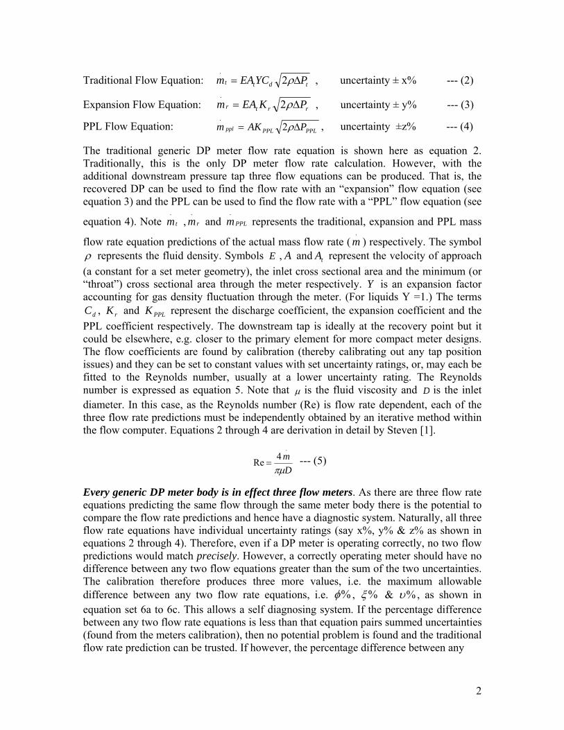
Fig 1. Orifice plate meter with instrumentation sketch and pressure fluctuation graph Figure 1 shows an orifice meter with instrumentation sketch and the (simplified) pressure fluctuation through the meter body. Traditional DP meters read the inlet pressure (P1), the downstream temperature (T) and the differential pressure (∆Pt) between the inlet pressure tap (1) and a pressure tap positioned at a point of low pressure (t). Note that the orifice meter in Figure 1 has a third pressure tap (d) downstream of the plate. This addition to the traditional DP meter design allows the measurement of two extra DP’s. That is, the differential pressure between the downstream (d) and the low (t) pressure taps (or “recovered” DP, ∆Pr) and the differential pressure between the inlet (1) and the downstream (d) pressure taps (i.e. the permanent pressure loss, ∆PPPL, sometimes called the “PPL” or “total head loss”). The sum of the recovered DP and the PPL equals the traditional differential pressure (equation 1). Hence, in order to obtain three DP’s, only two DP transmitters are required.
PPLrt PPP Δ+Δ=Δ --- (1)
2
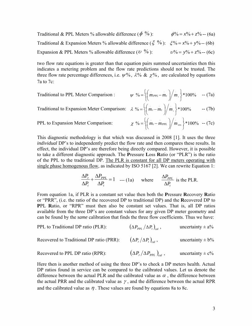
Traditional Flow Equation: tdtt PYCEAm Δ= ρ2.
, uncertainty ± x% --- (2)
Expansion Flow Equation: rrtr PKEAm Δ= ρ2.
, uncertainty ± y% --- (3)
PPL Flow Equation: PPLPPLppl PAKm Δ= ρ2.
, uncertainty ±z% --- (4) The traditional generic DP meter flow rate equation is shown here as equation 2. Traditionally, this is the only DP meter flow rate calculation. However, with the additional downstream pressure tap three flow equations can be produced. That is, the recovered DP can be used to find the flow rate with an “expansion” flow equation (see equation 3) and the PPL can be used to find the flow rate with a “PPL” flow equation (see
equation 4). Note tm.
, rm.
and PPLm.
represents the traditional, expansion and PPL mass
flow rate equation predictions of the actual mass flow rate (.
m ) respectively. The symbol ρ represents the fluid density. Symbols E , A and tA represent the velocity of approach (a constant for a set meter geometry), the inlet cross sectional area and the minimum (or “throat”) cross sectional area through the meter respectively. Y is an expansion factor accounting for gas density fluctuation through the meter. (For liquids Y =1.) The terms
dC , rK and PPLK represent the discharge coefficient, the expansion coefficient and the PPL coefficient respectively. The downstream tap is ideally at the recovery point but it could be elsewhere, e.g. closer to the primary element for more compact meter designs. The flow coefficients are found by calibration (thereby calibrating out any tap position issues) and they can be set to constant values with set uncertainty ratings, or, may each be fitted to the Reynolds number, usually at a lower uncertainty rating. The Reynolds number is expressed as equation 5. Note that μ is the fluid viscosity and D is the inlet diameter. In this case, as the Reynolds number (Re) is flow rate dependent, each of the three flow rate predictions must be independently obtained by an iterative method within the flow computer. Equations 2 through 4 are derivation in detail by Steven [1].
Dm
πμ
.4Re = --- (5)
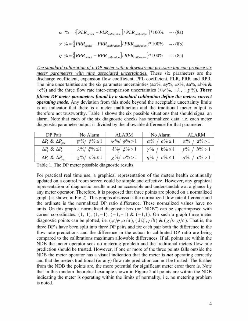
Every generic DP meter body is in effect three flow meters. As there are three flow rate equations predicting the same flow through the same meter body there is the potential to compare the flow rate predictions and hence have a diagnostic system. Naturally, all three flow rate equations have individual uncertainty ratings (say x%, y% & z% as shown in equations 2 through 4). Therefore, even if a DP meter is operating correctly, no two flow predictions would match precisely. However, a correctly operating meter should have no difference between any two flow equations greater than the sum of the two uncertainties. The calibration therefore produces three more values, i.e. the maximum allowable difference between any two flow rate equations, i.e. %φ , %ξ & %υ , as shown in equation set 6a to 6c. This allows a self diagnosing system. If the percentage difference between any two flow rate equations is less than that equation pairs summed uncertainties (found from the meters calibration), then no potential problem is found and the traditional flow rate prediction can be trusted. If however, the percentage difference between any
Expansion & PPL Meters % allowable difference ( %υ ): %%% zy +=υ -- (6c) two flow rate equations is greater than that equation pairs summed uncertainties then this indicates a metering problem and the flow rate predictions should not be trusted. The three flow rate percentage differences, i.e. %ψ , %λ & %χ , are calculated by equations 7a to 7c:
Traditional to PPL Meter Comparison : %100*%...
⎭⎬⎫
⎩⎨⎧
⎟⎠⎞
⎜⎝⎛ −= tmmm tPPLψ -- (7a)
Traditional to Expansion Meter Comparison: %100*%...
⎭⎬⎫
⎩⎨⎧
⎟⎠⎞
⎜⎝⎛ −= tmmm trλ -- (7b)
PPL to Expansion Meter Comparison: %100*%...
⎭⎬⎫
⎩⎨⎧
⎟⎠⎞
⎜⎝⎛ −= PPLmmm PPLrχ -- (7c)
This diagnostic methodology is that which was discussed in 2008 [1]. It uses the three individual DP’s to independently predict the flow rate and then compares these results. In effect, the individual DP’s are therefore being directly compared. However, it is possible to take a different diagnostic approach. The Pressure Loss Ratio (or “PLR”) is the ratio of the PPL to the traditional DP. The PLR is constant for all DP meters operating with single phase homogenous flow, as indicated by ISO 5167 [2]. We can rewrite Equation 1:
1=ΔΔ
+ΔΔ
t
PPL
t
r
PP
PP
--- (1a) where t
PPL
PPΔΔ
is the PLR.
From equation 1a, if PLR is a constant set value then both the Pressure Recovery Ratio or “PRR”, (i.e. the ratio of the recovered DP to traditional DP) and the Recovered DP to PPL Ratio, or “RPR” must then also be constant set values. That is, all DP ratios available from the three DP’s are constant values for any given DP meter geometry and can be found by the same calibration that finds the three flow coefficients. Thus we have:
PPL to Traditional DP ratio (PLR): ( )caltPPL PP ΔΔ , uncertainty ± a% Recovered to Traditional DP ratio (PRR): ( )caltr PP ΔΔ , uncertainty ± b% Recovered to PPL DP ratio (RPR): ( )calPPLr PP ΔΔ , uncertainty ± c% Here then is another method of using the three DP’s to check a DP meters health. Actual DP ratios found in service can be compared to the calibrated values. Let us denote the difference between the actual PLR and the calibrated value as α , the difference between the actual PRR and the calibrated value as γ , and the difference between the actual RPR and the calibrated value as η . These values are found by equations 8a to 8c.
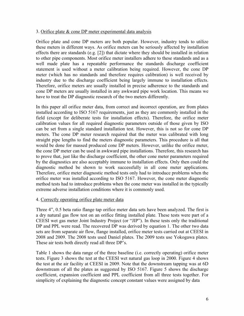
[ ]{ } %100*/% ncalibrationcalibratioactual RPRRPRRPR −=η --- (8c) The standard calibration of a DP meter with a downstream pressure tap can produce six meter parameters with nine associated uncertainties. These six parameters are the discharge coefficient, expansion flow coefficient, PPL coefficient, PLR, PRR and RPR. The nine uncertainties are the six parameter uncertainties (±x%, ±y%, ±z%, ±a%, ±b% & ±c%) and the three flow rate inter-comparison uncertainties (±ψ %, ±λ , ± χ %). These fifteen DP meter parameters found by a standard calibration define the meters correct operating mode. Any deviation from this mode beyond the acceptable uncertainty limits is an indicator that there is a meter malfunction and the traditional meter output is therefore not trustworthy. Table 1 shows the six possible situations that should signal an alarm. Note that each of the six diagnostic checks has normalized data, i.e. each meter diagnostic parameter output is divided by the allowable difference for that parameter.
DP Pair No Alarm ALARM No Alarm ALARM tPΔ & pplPΔ 1%% ≤φψ 1%% >φψ 1%% ≤aα 1%% >aα
tPΔ & rPΔ 1%% ≤ξλ 1%% >ξλ 1%% ≤bγ 1%% >bγ
rPΔ & pplPΔ 1%% ≤υχ 1%% >υχ 1%% ≤cη 1%% >cη Table 1. The DP meter possible diagnostic results. For practical real time use, a graphical representation of the meters health continually updated on a control room screen could be simple and effective. However, any graphical representation of diagnostic results must be accessible and understandable at a glance by any meter operator. Therefore, it is proposed that three points are plotted on a normalized graph (as shown in Fig 2). This graphs abscissa is the normalized flow rate difference and the ordinate is the normalized DP ratio difference. These normalized values have no units. On this graph a normalized diagnostic box (or “NDB”) can be superimposed with corner co-ordinates: (1, 1), (1, 1− ), ( 1− , 1− ) & ( 1− ,1). On such a graph three meter diagnostic points can be plotted, i.e. ( φψ , aα ), ( ξλ , bγ ) & ( υχ , cη ). That is, the three DP’s have been split into three DP pairs and for each pair both the difference in the flow rate predictions and the difference in the actual to calibrated DP ratio are being compared to the calibrations maximum allowable differences. If all points are within the NDB the meter operator sees no metering problem and the traditional meters flow rate prediction should be trusted. However, if one or more of the three points falls outside the NDB the meter operator has a visual indication that the meter is not operating correctly and that the meters traditional (or any) flow rate prediction can not be trusted. The further from the NDB the points are, the more potential for significant meter error there is. Note that in this random theoretical example shown in Figure 2 all points are within the NDB indicating the meter is operating within the limits of normality, i.e. no metering problem is noted.
5
Fig 2. A normalized diagnostic calibration box with normalized diagnostic result.
As both techniques use the same inputs, i.e. the three DP’s, it may be asked whether it is necessary to use both techniques together. If the DP relationships are as expected both techniques indicate no meter error. If they are not as expected both techniques should indicate incorrect meter operation. However, from experience (as we will see), it has been found that the two techniques can have slightly different sensitivities to problems. The DP ratio technique is more sensitive to metering abnormalities. Therefore, if both techniques show no problem then there is no alarm. If both techniques show a problem there is a “general alarm”. However, for relatively small problems the different sensitivities of the two methods can cause one technique to indicate a problem while the other indicates no problem. This scenario gives an “amber alarm”. The amber alarm indicates that there may be a metering problem. The amber alarm arises from the fact that the DP ratio technique can find real meter problems below the flow rate comparison techniques sensitivity limit. However, there are rare cases where the DP ratio technique is too sensitive to real but very small problems that do not cause the flow rate prediction to be beyond the meters stated uncertainty. However, the flow rate comparison technique is never sensitive enough to trigger such a false alarm. Therefore, the flow rate comparison technique can counter any over sensitivity of the DP ratio technique by offering the operator objectivity. The amber alarm states that there is a possibility of a small metering problem, but if it exists the metering error is correspondingly small. Therefore, it is beneficial to use both techniques simultaneously (especially as the computational power required is relatively small). We shall now look at orifice and cone meter correct and incorrect operation data to show the usefulness of these methodologies.
Fig 2a. Normalized diagnostic box with alarm zones.
6
3. Orifice plate & cone DP meter experimental data analysis Orifice plate and cone DP meters are both popular. However, industry tends to utilize these meters in different ways. As orifice meters can be seriously affected by installation effects there are standards (e.g. [2]) that dictate where they should be installed in relation to other pipe components. Most orifice meter installers adhere to these standards and as a well made plate has a repeatable performance the standards discharge coefficient statement is used without a meter calibration being required. However, the cone DP meter (which has no standards and therefore requires calibration) is well received by industry due to the discharge coefficient being largely immune to installation effects. Therefore, orifice meters are usually installed in precise adherence to the standards and cone DP meters are usually installed in any awkward pipe work location. This means we have to treat the DP diagnostic research of the two meters differently. In this paper all orifice meter data, from correct and incorrect operation, are from plates installed according to ISO 5167 requirements, just as they are commonly installed in the field (except for deliberate tests for installation effects). Therefore, the orifice meter calibration values for all required diagnostic parameters outside of those given by ISO can be set from a single standard installation test. However, this is not so for cone DP meters. The cone DP meter research required that the meter was calibrated with long straight pipe lengths to find the meters diagnostic parameters. This procedure is all that would be done for massed produced cone DP meters. However, unlike the orifice meter, the cone DP meter can be used in awkward pipe installations. Therefore, this research has to prove that, just like the discharge coefficient, the other cone meter parameters required by the diagnostics are also acceptably immune to installation effects. Only then could the diagnostic method be shown to work successfully in all cone meter applications. Therefore, orifice meter diagnostic method tests only had to introduce problems when the orifice meter was installed according to ISO 5167. However, the cone meter diagnostic method tests had to introduce problems when the cone meter was installed in the typically extreme adverse installation conditions where it is commonly used. 4. Correctly operating orifice plate meter data Three 4”, 0.5 beta ratio flange tap orifice meter data sets have been analyzed. The first is a dry natural gas flow test on an orifice fitting installed plate. These tests were part of a CEESI wet gas meter Joint Industry Project (or “JIP”). In these tests only the traditional DP and PPL were read. The recovered DP was derived by equation 1. The other two data sets are from separate air flow, flange installed, orifice meter tests carried out at CEESI in 2008 and 2009. The 2008 tests used Daniel plates. The 2009 tests use Yokogawa plates. These air tests both directly read all three DP’s. Table 1 shows the data range of the three baseline (i.e. correctly operating) orifice meter tests. Figure 3 shows the test at the CEESI wet natural gas loop in 2000. Figure 4 shows the test at the air facility at CEESI in 2009. Note that the downstream tapping was at 6D downstream of all the plates as suggested by ISO 5167. Figure 5 shows the discharge coefficient, expansion coefficient and PPL coefficient from all three tests together. For simplicity of explaining the diagnostic concept constant values were assigned by data
7
Fig 3. Orifice fitting with natural gas flow. Fig 4. Flange installed plate with air flow.
Test 2000 Natural Gas 2008 Air 2009 Air Orifice Type & Fit Daniel Orifice Fitting Daniel Plate / Flange Yokogawa Plate /Flange No. of data points 112 44 124
Pressure Range 13.1 < P (bar) < 87.0 15.0 < P (bar) < 30.0 14.9 < P (bar) < 30.1 DPt Range 10”WC< DPt <400”WC 15”WC< DPt < 385”WC 15”WC< DPt < 376”WC DPr Range 10”WC <DPr < 106”WC 10”WC < DPr < 100”WC 10”WC <DPr < 100”WC
DPppl Range 10”WC <PPL < 293”WC 11”WC<PPL< 285”WC 11”WC<PPL< 277”WC Reynolds No. Range 350 e3 < Re < 8.1e6 300e3 < Re < 2.1e6 317e3 < Re < 2.2e6 Table 1. The three orifice plate meter baseline data sets. fitting. (It should be noted that more than 95% of the combined discharge coefficient results fitted the Reader Harris –Gallagher, or “RHG”, equation to within this equations stated uncertainty bands of ±0.5%.) All three flow coefficient constant values are given in Figure 5 with a stated uncertainty at 95% confidence. Figure 6 shows the PLR, PRR & RPR from all three tests together. Constant values were assigned by analysis of the combined data and are shown in Figure 6 with a stated uncertainty at 95% confidence. Note that the sum of the PLR and PRR is not quite unity as theoretically required due to data uncertainty. Figures 5 & 6 indicate that all six parameters exist as set values at relatively low uncertainty and they are repeatable and reproducible. Fig 7 shows the full results of calibrating this DP meter type with a downstream pressure tap. The boxed information shows the traditional DP meter calibration result, i.e. the discharge coefficient and its uncertainty to 95% confidence. The broken line box indicates a rare additional traditional result when a downstream pressure tap is included. Note even in this rare case when a downstream tap is included, only the PLR is found. Traditionally no other parameter is considered and the downstream tap only exists to help predict the PPL across the component for overall PPL predictions on the piping system. Fig 7 shows that all fifteen DP meter parameters discussed in the theory exist in reality. From adding an extra pressure tap and DP transmitter, a standard DP meter calibration run can find each of the DP meters fifteen parameters. Each parameter tells the meter user something unique and of interest about the nature of that meters response to the flow. That is, a DP Diagnostics meter calibration produces several times the standard calibration information from effectively the same effort and expense.
8
Fig 5. Combined 4”, 0.5 beta ratio orifice plate meter flow coefficient results.
Fig 6. Combined 4”, 0.5 beta ratio orifice plate meter DP ratio results.
Fig 7. The results of a full DP meter calibration.
In reality most orifice meters are not calibrated. ISO 5167 provides the RHG equation to find the discharge coefficient (Cd) and the associated uncertainty (±x%). It also offers a couple of PLR equations although no uncertainty (±a%) for these equations are given. The ISO PLR equation considered as more precise is equation 9:
9
( ){ }( ){ } 224
224
11
11
ββ
ββ
dd
dd
CC
CCPLR
+−−
−−−= -- (9) PLRPRR −=1 -- (10)
PLRPRRRPR = -- (11)
Therefore, as ISO offers a PLR equation, there are associated predictions for PRR (equation 10) and RPR (equation 11), although of course ISO does not state as much. Furthermore, it can be shown that:
PLRCK d
r −=
1ε
--- (12) PLR
CEK dppl
εβ 2
= --- (13)
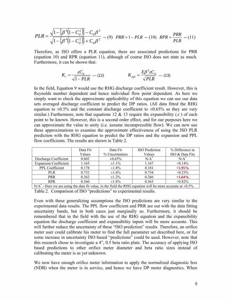
In the field, Equation 9 would use the RHG discharge coefficient result. However, this is Reynolds number dependent and hence individual flow point dependent. As here we simply want to check the approximate applicability of this equation we can use our data sets averaged discharge coefficient to predict the DP ratios. (All data fitted the RHG equation to ±0.5% and the constant discharge coefficient to ±0.65% so they are very similar.) Furthermore, note that equations 12 & 13 require the expansibility (ε ) of each point to be known. However, this is a second order effect, and for our purposes here we can approximate the value to unity (i.e. assume incompressible flow). We can now use these approximations to examine the approximate effectiveness of using the ISO PLR prediction with the RHG equation to predict the DP ratios and the expansion and PPL flow coefficients. The results are shown in Table 2. Data Fit
N/A* - Here we are using the data fit value, in the field the RHG equation will be more accurate at ±0.5%. Table 2. Comparison of ISO “predictions” to experimental results. Even with these generalizing assumptions the ISO predictions are very similar to the experimental data results. The PPL flow coefficient and PRR are out with the data fitting uncertainty bands, but in both cases just marginally so. Furthermore, it should be remembered that in the field with the use of the RHG equation and the expansibility equation the discharge coefficient and expansibility inputs will be more accurate. This will further reduce the uncertainty of these “ISO prediction” results. Therefore, an orifice meter user could calibrate his meter to find the full parameter set described here, or for some increase in uncertainty ISO based “predictions” could be used. However, note that this research chose to investigate a 4”, 0.5 beta ratio plate. The accuracy of applying ISO based predictions to other orifice meter diameter and beta ratio sizes instead of calibrating the meter is as yet unknown. We now have enough orifice meter information to apply the normalized diagnostic box (NDB) when the meter is in service, and hence we have DP meter diagnostics. When
10
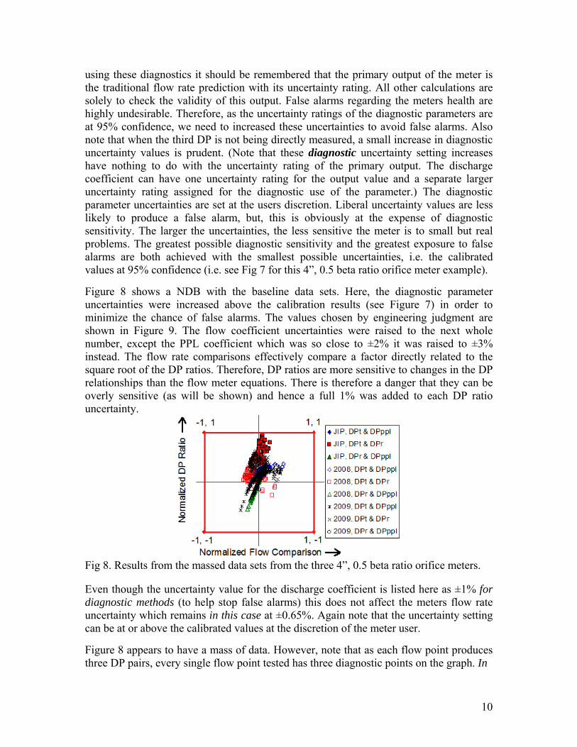
using these diagnostics it should be remembered that the primary output of the meter is the traditional flow rate prediction with its uncertainty rating. All other calculations are solely to check the validity of this output. False alarms regarding the meters health are highly undesirable. Therefore, as the uncertainty ratings of the diagnostic parameters are at 95% confidence, we need to increased these uncertainties to avoid false alarms. Also note that when the third DP is not being directly measured, a small increase in diagnostic uncertainty values is prudent. (Note that these diagnostic uncertainty setting increases have nothing to do with the uncertainty rating of the primary output. The discharge coefficient can have one uncertainty rating for the output value and a separate larger uncertainty rating assigned for the diagnostic use of the parameter.) The diagnostic parameter uncertainties are set at the users discretion. Liberal uncertainty values are less likely to produce a false alarm, but, this is obviously at the expense of diagnostic sensitivity. The larger the uncertainties, the less sensitive the meter is to small but real problems. The greatest possible diagnostic sensitivity and the greatest exposure to false alarms are both achieved with the smallest possible uncertainties, i.e. the calibrated values at 95% confidence (i.e. see Fig 7 for this 4”, 0.5 beta ratio orifice meter example). Figure 8 shows a NDB with the baseline data sets. Here, the diagnostic parameter uncertainties were increased above the calibration results (see Figure 7) in order to minimize the chance of false alarms. The values chosen by engineering judgment are shown in Figure 9. The flow coefficient uncertainties were raised to the next whole number, except the PPL coefficient which was so close to ±2% it was raised to ±3% instead. The flow rate comparisons effectively compare a factor directly related to the square root of the DP ratios. Therefore, DP ratios are more sensitive to changes in the DP relationships than the flow meter equations. There is therefore a danger that they can be overly sensitive (as will be shown) and hence a full 1% was added to each DP ratio uncertainty.
Fig 8. Results from the massed data sets from the three 4”, 0.5 beta ratio orifice meters. Even though the uncertainty value for the discharge coefficient is listed here as ±1% for diagnostic methods (to help stop false alarms) this does not affect the meters flow rate uncertainty which remains in this case at ±0.65%. Again note that the uncertainty setting can be at or above the calibrated values at the discretion of the meter user.
Figure 8 appears to have a mass of data. However, note that as each flow point produces three DP pairs, every single flow point tested has three diagnostic points on the graph. In
11
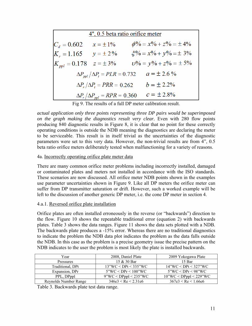
Fig 9. The results of a full DP meter calibration result.
actual application only three points representing three DP pairs would be superimposed on the graph making the diagnostics result very clear. Even with 280 flow points producing 840 diagnostic results in Figure 8, it is clear that no point for these correctly operating conditions is outside the NDB meaning the diagnostics are declaring the meter to be serviceable. This result is in itself trivial as the uncertainties of the diagnostic parameters were set to this very data. However, the non-trivial results are from 4”, 0.5 beta ratio orifice meters deliberately tested when malfunctioning for a variety of reasons. 4a. Incorrectly operating orifice plate meter data There are many common orifice meter problems including incorrectly installed, damaged or contaminated plates and meters not installed in accordance with the ISO standards. These scenarios are now discussed. All orifice meter NDB points shown in the examples use parameter uncertainties shown in Figure 9. Like all DP meters the orifice meter can suffer from DP transmitter saturation or drift. However, such a worked example will be left to the discussion of another generic DP meter, i.e. the cone DP meter in section 4. 4.a.1. Reversed orifice plate installation Orifice plates are often installed erroneously in the reverse (or “backwards”) direction to the flow. Figure 10 shows the repeatable traditional error (equation 2) with backwards plates. Table 3 shows the data ranges. Figure 11 shows the data sets plotted with a NDB. The backwards plate produces a -15% error. Whereas there are no traditional diagnostics to indicate the problem the NDB data plot indicates the problem as the data falls outside the NDB. In this case as the problem is a precise geometry issue the precise pattern on the NDB indicates to the user the problem is most likely the plate is installed backwards.
Year 2008, Daniel Plate 2009 Yokogawa Plate Pressures 15 & 30 Bar 15 Bar
PPL, DPppl 9”WC < DPppl < 235”WC 10”WC < DPppl < 229”WC Reynolds Number Range 346e3 < Re < 2.31e6 367e3 < Re < 1.66e6
Table 3. Backwards plate test data range.
12
Fig 10. Reproducible significant errors when plate is installed backwards.
Fig 11. Graph indicating metering error with NDB and all reversed plate results.
4.a.2. Damaged orifice plates – buckled (or “warped”) plates Adverse flow conditions can damage orifice plates. A buckled plate can give significant flow measurement errors. Traditionally there is no diagnostic methodology to indicate this problem. In 2008 DP Diagnostics heavily damaged a 4”, 0.5 beta plate to show the diagnostic capability of the downstream tap. In 2009 this test was re-run to prove repeatability of the new diagnostic system. Then a more moderately buckled 4”, 0.5 beta ratio plate was tested. The buckled plates are shown in Figures 12 & 13. Table 4 shows the test data ranges. Figure 14 shows the flow rate prediction (equation 2) error due to the buckling. The heavily buckle produces a -30% error. The moderate buckle plate produces
Test 2008, Severe Buckle 2009, Severe Buckle 2009, Moderate Buckle Pressures 15 & 30 Bar 15 & 30 Bar 15 & 30Bar
Fig 14. Flow rate prediction errors due to buckled orifice plates.
Fig 15. Metering error with NDB Fig 16. Metering error with NDB & heavily buckled plate results. & moderately buckled plate results. a -7% error. The pressure had no effect on the results and the results were very repeatable. Figure 15 shows the heavily buckled plate data sets plotted with a NDB.
14
Figure 16 shows the moderately buckled plate data set plotted with a NDB. This indicates a significant problem. Note that for the moderately buckled plate the traditional and PPL DP pair does not trigger the alarm. However, all three DP pairs are always available and the other two DP pairs clearly trigger the alarm. This example highlights the extreme usefulness of the traditionally least used DP, i.e. recovered DP. (In fact, the particular DP pair to trigger any alarm is wholly dependent on the meter design the type of problem.) 4.a.3. Damaged orifice plate – worn leading orifice edge Orifice sharp edges can be worn leading to flow measurement errors. Traditionally there is no diagnostic methodology to indicate this problem. In 2008 DP Diagnostics heavily filed down a 4”, 0.5 beta orifice edge to show the diagnostic capability of the downstream tap. In 2009 smaller damage was tested with 0.01” and 0.02” chamfers being put on 4”, 0.5 beta orifice edges. The filed and 0.01” chamfer are shown in Figures 17 & 18. Table 5 shows the test data ranges. Figure 19 shows the flow rate prediction (equation 2) error due to the orifice edge wear. The approximate errors are -8% for the heavily filed orifice edge, -5% for the 0.02” chamfered edge and -2.5% for the 0.01” chamfered edge. Figure 20 shows the “worn” plate data sets plotted with a NDB. (Pressure had no effect on the results so both pressures tested are shown as one data set, i.e. three DP pairs, per plate.) In Figure 20 the data plotted on a NDB shows the heavily filed edge plate to have significant problems. In Figure 21 the larger chamfer also has a clear diagnostic indication that there are significant problems. Therefore these meter flow rate outputs should not be trusted. It is interesting to again note that not all three DP pairs always trip an alarm. Here the traditional DP and PPL pairings again do not always see the problem and again it is the rarest used of the DP’s, i.e. the recovery DP, used with either of the other two DP’s that is correctly tripping the alarm. Finally, note that as would be expected, the smallest edge damage (i.e. the 0.01” chamfer) is the most difficult to notice. With a traditional flow rate error of only -2.5% the traditional and recovery DP ratio just picks up the problem. The other two DP pairs are not sensitive enough to this particular problem to trigger an alarm. This appears to be the limit of the diagnostic systems ability. A smaller amount of damage (say causing a metering error < 2%) may not be seen.
4.026", 0.5 Beta Ratio Orifice Plate Meter
-0.5%
+0.5%
-10-8-6-4-202468
10
0 500000 1000000 1500000 2000000 2500000Pipe Reynolds Number
PPL, DPppl 10”WC <DPr< 256”WC 10”WC<DPppl< 256”WC 11”WC<DPppl<270”WC Reynolds No. Range 325e3 < Re < 2.23e6 352e3 < Re < 2.15e6 332e3 < Re < 2.12e6
Table 5. Worn orifice plate edge test data range.
Fig 20. Metering error with NDB Fig 21. Metering error with NDB and & heavily filed orifice edge results. chamfered orifice edge plate results. 4.a.4. Contaminated orifice plates Adverse flow conditions can deposit contaminates on orifice plates leading to flow measurement errors. Traditionally there are no diagnostics to indicate this problem. There are two types of contamination. There is fluid contamination (e.g. oil from upstream components) which is transient in nature, and difficult to test, and the more stable and easier to test case of solid deposits left on plates. Therefore, two 4”, 0.5 beta plates were given mild and severe contamination respectively. The mildly contaminated plate was lightly spray painted on the upstream side to produce light ripples and some paint drops at the sharp edge. The heavily contaminated plate was heavily painted on the upstream side and then large salt granules embedded in the painted to produce an extremely rough surface. Due to time and financial constraints no downstream side plate contamination was investigated. The contaminated plates are shown in Figures 22 & 23 respectively.
16
Fig 22. Lightly contamination. Fig 23. Heavy contamination.
Test 2008, Mild Contamination 2009, Heavy Contamination Pressures 15 & 30 Bar 15 & 30 Bar
PPL, DPppl 11”WC <DPppl< 276”WC 12”WC<DPppl< 265”WC Reynolds No. Range 318e3 < Re < 2.18e6 346e3 < Re < 2.15e6
Table 6. Contaminated plate test data range.
Fig 24. Flow rate prediction errors due to contamination on orifice plates. Table 6 shows the test data ranges. Figure 24 shows the flow rate prediction (equation 2) errors of -4% and -1.5% for the heavily and lightly contaminated plates respectively. These results are similar to fluid contamination test results by Johansen [3] and Pritchard [4]. Figure 25 shows the two data sets plotted with a NDB. Again, as pressure had no effect, both pressures tested for each plate are simply shown as one data set, i.e. three DP pairs, per plate. Figure 25 shows the heavily contaminated plate to have problems so the meters flow rate output should not be trusted. Again note that the traditional DP and PPL pairings do not see the heavy contamination problem and again it is the recovery DP, used with either of
17
Fig 25. Graph indicating metering error with NDB and all contaminated plate results.
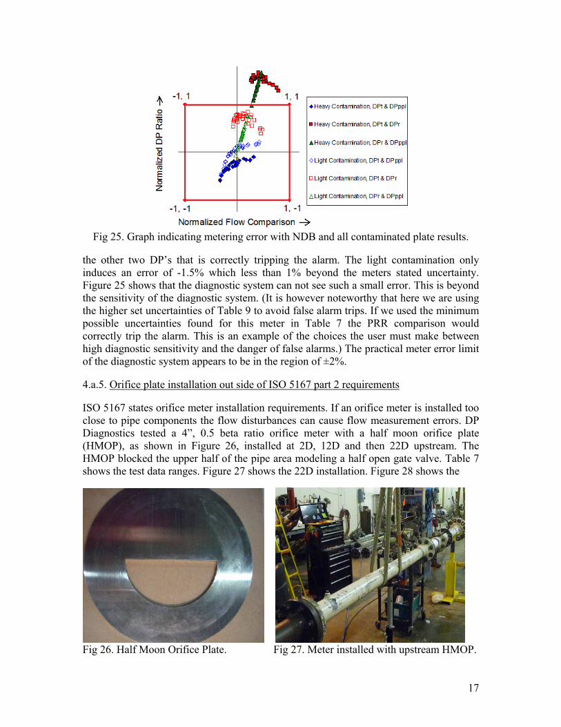
the other two DP’s that is correctly tripping the alarm. The light contamination only induces an error of -1.5% which less than 1% beyond the meters stated uncertainty. Figure 25 shows that the diagnostic system can not see such a small error. This is beyond the sensitivity of the diagnostic system. (It is however noteworthy that here we are using the higher set uncertainties of Table 9 to avoid false alarm trips. If we used the minimum possible uncertainties found for this meter in Table 7 the PRR comparison would correctly trip the alarm. This is an example of the choices the user must make between high diagnostic sensitivity and the danger of false alarms.) The practical meter error limit of the diagnostic system appears to be in the region of ±2%. 4.a.5. Orifice plate installation out side of ISO 5167 part 2 requirements ISO 5167 states orifice meter installation requirements. If an orifice meter is installed too close to pipe components the flow disturbances can cause flow measurement errors. DP Diagnostics tested a 4”, 0.5 beta ratio orifice meter with a half moon orifice plate (HMOP), as shown in Figure 26, installed at 2D, 12D and then 22D upstream. The HMOP blocked the upper half of the pipe area modeling a half open gate valve. Table 7 shows the test data ranges. Figure 27 shows the 22D installation. Figure 28 shows the
Fig 26. Half Moon Orifice Plate. Fig 27. Meter installed with upstream HMOP.
18
Test 2D upstream 12D upstream 22D upstream Pressures 15 Bar 15 Bar 15 Bar
PPL, DPppl 11”WC <DPr< 281”WC 14”WC<DPppl< 301”WC 23”WC <DPr< 280”WC Reynolds No. Range 323e3 < Re < 1.52e6 373e3 < Re < 1.66e6 455e3 < Re < 1.52e6
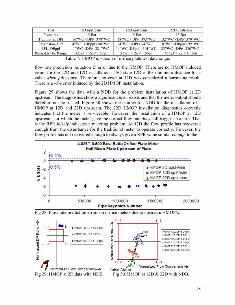
Table 7. HMOP upstream of orifice plate test data range. flow rate prediction (equation 2) error due to the HMOP. There are no HMOP induced errors for the 22D and 12D installations. ISO state 12D is the minimum distance for a valve when fully open. Therefore, no error at 12D was considered a surprising result. There is a -6% error induced by the 2D HMOP installation. Figure 29 shows the data with a NDB for the problem installation of HMOP at 2D upstream. The diagnostics show a significant error exists and that the meter output should therefore not be trusted. Figure 30 shows the data with a NDB for the installation of a HMOP at 12D and 22D upstream. The 22D HMOP installation diagnostics correctly indicates that the meter is serviceable. However, the installation of a HMOP at 12D upstream, for which the meter gave the correct flow rate does still trigger an alarm. That is the RPR falsely indicates a metering problem. At 12D the flow profile has recovered enough from the disturbance for the traditional meter to operate correctly. However, the flow profile has not recovered enough to always give a RPR value similar enough to the
Fig 28. Flow rate prediction errors on orifice meters due to upstream HMOP’s.
Fig 29. HMOP at 2D data with NDB. Fig 30. HMOP at 12D & 22D with NDB.
19
calibrated value. That is, the RPR is too sensitive to the flow disturbance here, and it is therefore suggesting there is a metering problem when in fact there is not. This is the reason why general and amber alarms are proposed. It should be realized that a HMOP 12D upstream of an orifice meter is an extremely poor installation which is very rare in reality. DP Diagnostics has primarily developed the diagnostics for use with correctly installed orifice plate meters in which this is not. With that said, if this meter was calibrated in-situ the effect of the disturbance could be calibrated out of the diagnostic parameters. It is also of interest to note that it was found after analysis, that if the uncertainty rating of the RPR had been chosen as 4% instead of 2.8% the alarm warning would not have triggered and all other diagnostic results for correctly and incorrectly operating orifice meters would also have remained correct. However, this would be fitting the uncertainties with the benefit of hindsight which does not give a realistic review of the ability of the diagnostics, so the original research results are kept here. The issue here is that this is a new diagnostic methodology, and the best parameter uncertainty settings which produce the best balance between an over sensitive system and a system that is too insensitive will need to be found by experience. 4.b. A review of the orifice meter diagnostic system test results A general alarm almost certainly indicates a significant metering problem. An amber alarm very probably indicates either a significant or small metering problem. In reality for any generic DP meter there is virtually no chance of an amber alarm being triggered by a flow rate comparison while the associated DP ratio comparison does not trigger the alarm. This is due to the DP ratios being more sensitive to problems than the flow rate comparisons technique. Therefore, an amber alarm is going to be triggered by the DP ratio technique only. Note that the user can make engineering judgments on these alarms. There are three points of interest while judging if an amber alarm indicates a real problem and if so, is the error significant enough to merit intervention? 1. How far outside the NDB are the points? The further outside the NDB the more chance of a significant real problem. In practical terms the amber alarm can be limited to the case where the DP ratio comparison alarm values are between 1 and 1.5. Beyond the 1.5 value all experimental results show a significant real metering error. 2. Is there more than one point outside the NDB? If so the chances of a real significant problem are increased. 3. If a DP ratio point is outside the NDB, where is it located on the abscissa? The further from the ordinate, the closer the flow rate comparison technique is to signaling a general alarm and the more likely then that the amber alarm is indicating a real and significant metering problem. 5. Correctly operating ∆P cone meter data The diagnostic methods described in Section 2 are available for all generic DP meter designs. In this section the cone DP meter is discussed. A sketch of a cone DP meter design and the pressure fluctuations through the meter is given in Figure 31. Note the extreme similarity to the orifice meter sketch in Figure 1.
20
Fig 31. Cone meter with instrumentation sketch and pressure fluctuation graph DP Diagnostics built and tested a 4”, 0.63 beta ratio cone meter (with a downstream tap). The centre line of the cone support is 2D from the inlet flange face and 5.25D from the outlet flange face (as the meter is 7.25D long). The three DP’s were read directly. The meter was fully calibrated (at 14 & 41 Bar) with straight lengths upstream and downstream (see Figure 33). The results are shown in Figure 32. Table 8 shows these baseline test data ranges. The discharge coefficient was found to ±1/2% as expected. Again, the other parameters were found to be of a relatively low uncertainty.
Test Baseline Adverse Flow Conditions Pressure Range 17.2 < P (bar) < 41.1 17.2 bar
DPt Range 21”WC< DPt <301”WC 14”WC< DPt < 304”WC DPr Range 10”WC <DPr < 133”WC 6”WC < DPr < 136”WC
DPppl Range 12”WC <PPL < 169”WC 7”WC<PPL< 168”WC Reynolds No. Range 888 e3 < Re < 3.75e6 734e3 < Re < 2.9e6
Fig 32. The results of the standard straight run DP cone meter calibration.
Cone DP meters are popular due to their discharge coefficients proven immunity to flow disturbances. Hence, after calibration it was necessary to test the meter with a myriad of adverse flow conditions in order to prove that all the diagnostic parameters are acceptably immune to flow disturbances and therefore the ∆P Cone Meter has a practical diagnostic capability. The adverse flow conditions tested were a double out of plane bend (DOPB) at 0D (Figure 34), 2D & 5D upstream, a DOPB at 0D upstream with a half moon orifice plate (HMOP) at 2D downstream (Figure 35), a DOPB at 0D upstream and a triple out of plane bend (TOPB) 0D downstream (Figure 36), a HMOP 6.7D & then 8.7D upstream (Figures 37 & 38), a HMOP 2D downstream (Figure 39) and a 540 swirl
21
Fig 33. Baseline Fig 34. DOPB, 0D up
Fig 35. DOPB 0D up & HMOP 2D down Fig 36. DOPB 0D up & TOPB down
Fig 37. HMOP 6.7D up Fig 38. HMOP 8.7D up generator with a 3” to 4” expansion 9D upstream (Figure 40). Very few real applications would create worse flow conditions at the meter inlet. Table 8 shows the test data ranges. Figure 41 shows the disturbance effects on the discharge coefficient. Two installations cause it to vary beyond the baseline ±½% uncertainty. They are the HMOP 6.7D and
swirl generator with expander upstream installations. Both installations are extreme. The HMOP at 6.7D models a gate valve at 5D upstream. This is below the minimum
22
Fig 39. HMOP 2D down Fig 40. 3” Swirl Generator + Expansion 9D up
Cd = 0.803,+/-1% to 95% confidence+0.5%
-0.5%
+1%
-1%
0.76
0.77
0.78
0.79
0.8
0.81
0.82
0 500000 1000000 1500000 2000000 2500000 3000000 3500000 4000000Reynolds Number
Dis
char
ge C
oeffi
cien
t
BaselineDouble Out of Plane Bend 0D upstreamDouble Out of Plane Bend 2D upstreamDouble Out of Plane Bend 5D upstreamDouble Out of Plane Bend 0D upstream, Half Moon Plate 2D dow nstreamDouble Out of Plane Bend 0D upstream, Triple Out of Plane Bend 0D dow nstreamHalf Moon Plate 6.7D upstreamHalf Moon Plate 8.7D upstreamHalf Moon Plate 2D dow nstreamSw irl Generator w ith 3" to 4" Expansion 9D upstream
Fig 41. 4”, 0.63 beta ratio, ∆P cone meter disturbed flow discharge coefficient results. recommended upstream distance (of 6D) for this meter. The HMOP at 6.7D increases the discharge coefficient by approximately 0.8%. Extending the upstream distance to 8.7D (i.e. a gate valve at 7D) drops the discharge coefficient to with the baseline uncertainty. The extreme swirl with expansion 9D upstream dropped the discharge coefficient below the baseline uncertainty at lower Reynolds numbers. Even so all discharge coefficient data from all the disturbance tests are spread around the baseline calibrated value to ±1% at 95% confidence. (Nevertheless, DP Diagnostics suggests valves are installed no closer then 7D upstream of cone meters and inlet swirl conditions are limited to moderate swirl, say <300, especially if there is an expansion close by upstream.) Figures 42 & 43 show the disturbance effect on all the flow coefficient and DP ratios. All parameters are more affected than the discharge coefficient, but, crucially they are still relatively immune to disturbances. Commercial ∆P cone meters would be calibrated with straight pipe lengths only, so the baseline flow coefficient and DP ratio results must be held and only the uncertainty limits changed (i.e. increased) by standard agreed amounts to account for the possible real world use in extreme installations. It is proposed here that the standard uncertainties assigned to the calibration found diagnostic parameter values are those found in these extreme tests. Therefore the 15 parameters defining this ∆P cone
23
Fig 42. Flow coefficient disturbance test results for the 4”, 0.63 beta ratio ∆P cone meter.
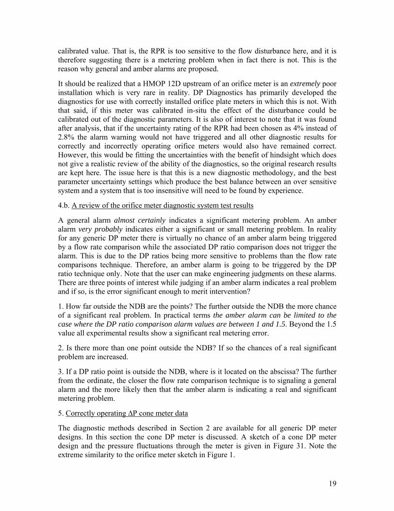
Fig 43. DP ratio disturbance test results for the 4”, 0.63 beta ratio ∆P cone meter. meter are as shown in Figure 44. With the six diagnostic parameters and the nine associated uncertainties set, all baseline data sets (minus the 6.7D HMOP which is below the minimum distance allowed) can now be plotted on a NDB (see Figure 45). By design all points for the correctly operating meter are within the NDB. For a far more detailed discussion on these test results see Steven [5].
24
Fig 44. The ∆P cone meter diagnostic parameters and practical uncertainties.
Fig 45. All correctly operating 4”, 0.63 beta ratio ∆P cone meter data with a NDB.
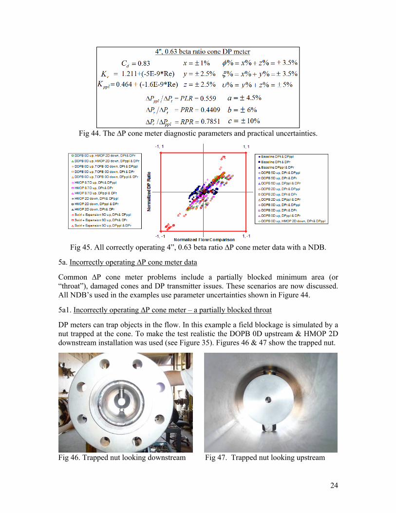
5a. Incorrectly operating ∆P cone meter data Common ∆P cone meter problems include a partially blocked minimum area (or “throat”), damaged cones and DP transmitter issues. These scenarios are now discussed. All NDB’s used in the examples use parameter uncertainties shown in Figure 44. 5a1. Incorrectly operating ∆P cone meter – a partially blocked throat DP meters can trap objects in the flow. In this example a field blockage is simulated by a nut trapped at the cone. To make the test realistic the DOPB 0D upstream & HMOP 2D downstream installation was used (see Figure 35). Figures 46 & 47 show the trapped nut.
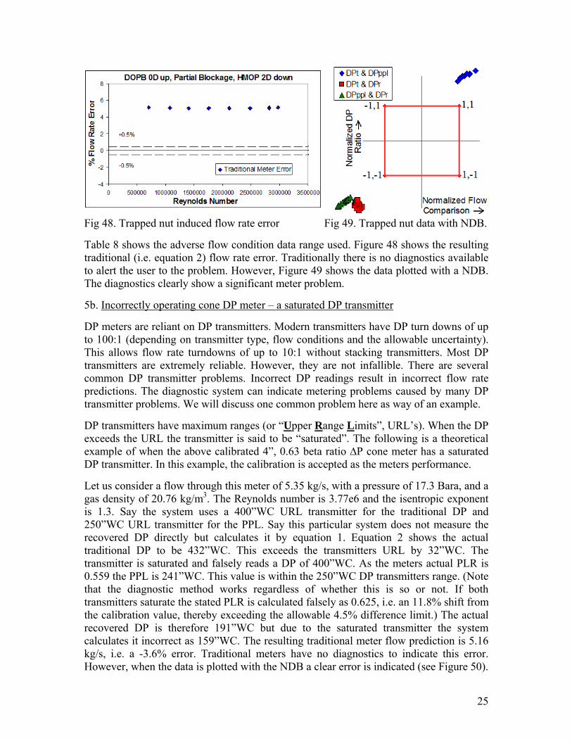
Fig 48. Trapped nut induced flow rate error Fig 49. Trapped nut data with NDB. Table 8 shows the adverse flow condition data range used. Figure 48 shows the resulting traditional (i.e. equation 2) flow rate error. Traditionally there is no diagnostics available to alert the user to the problem. However, Figure 49 shows the data plotted with a NDB. The diagnostics clearly show a significant meter problem. 5b. Incorrectly operating cone DP meter – a saturated DP transmitter DP meters are reliant on DP transmitters. Modern transmitters have DP turn downs of up to 100:1 (depending on transmitter type, flow conditions and the allowable uncertainty). This allows flow rate turndowns of up to 10:1 without stacking transmitters. Most DP transmitters are extremely reliable. However, they are not infallible. There are several common DP transmitter problems. Incorrect DP readings result in incorrect flow rate predictions. The diagnostic system can indicate metering problems caused by many DP transmitter problems. We will discuss one common problem here as way of an example. DP transmitters have maximum ranges (or “Upper Range Limits”, URL’s). When the DP exceeds the URL the transmitter is said to be “saturated”. The following is a theoretical example of when the above calibrated 4”, 0.63 beta ratio ∆P cone meter has a saturated DP transmitter. In this example, the calibration is accepted as the meters performance. Let us consider a flow through this meter of 5.35 kg/s, with a pressure of 17.3 Bara, and a gas density of 20.76 kg/m3. The Reynolds number is 3.77e6 and the isentropic exponent is 1.3. Say the system uses a 400”WC URL transmitter for the traditional DP and 250”WC URL transmitter for the PPL. Say this particular system does not measure the recovered DP directly but calculates it by equation 1. Equation 2 shows the actual traditional DP to be 432”WC. This exceeds the transmitters URL by 32”WC. The transmitter is saturated and falsely reads a DP of 400”WC. As the meters actual PLR is 0.559 the PPL is 241”WC. This value is within the 250”WC DP transmitters range. (Note that the diagnostic method works regardless of whether this is so or not. If both transmitters saturate the stated PLR is calculated falsely as 0.625, i.e. an 11.8% shift from the calibration value, thereby exceeding the allowable 4.5% difference limit.) The actual recovered DP is therefore 191”WC but due to the saturated transmitter the system calculates it incorrect as 159”WC. The resulting traditional meter flow prediction is 5.16 kg/s, i.e. a -3.6% error. Traditional meters have no diagnostics to indicate this error. However, when the data is plotted with the NDB a clear error is indicated (see Figure 50).
26
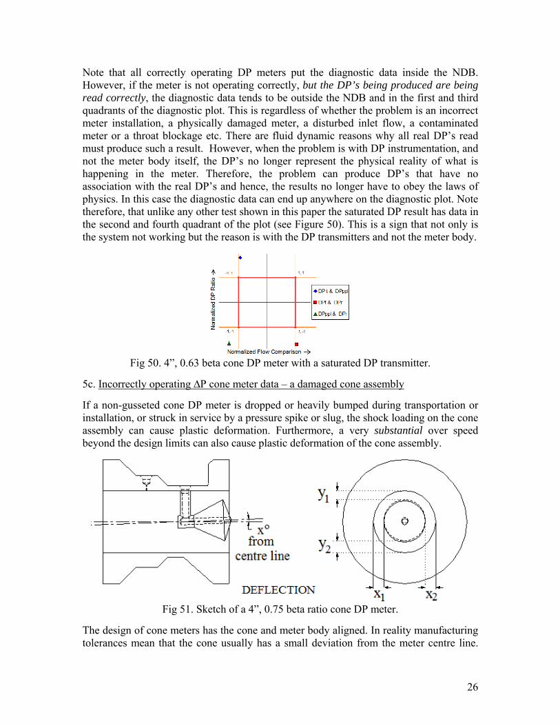
Note that all correctly operating DP meters put the diagnostic data inside the NDB. However, if the meter is not operating correctly, but the DP’s being produced are being read correctly, the diagnostic data tends to be outside the NDB and in the first and third quadrants of the diagnostic plot. This is regardless of whether the problem is an incorrect meter installation, a physically damaged meter, a disturbed inlet flow, a contaminated meter or a throat blockage etc. There are fluid dynamic reasons why all real DP’s read must produce such a result. However, when the problem is with DP instrumentation, and not the meter body itself, the DP’s no longer represent the physical reality of what is happening in the meter. Therefore, the problem can produce DP’s that have no association with the real DP’s and hence, the results no longer have to obey the laws of physics. In this case the diagnostic data can end up anywhere on the diagnostic plot. Note therefore, that unlike any other test shown in this paper the saturated DP result has data in the second and fourth quadrant of the plot (see Figure 50). This is a sign that not only is the system not working but the reason is with the DP transmitters and not the meter body.
Fig 50. 4”, 0.63 beta cone DP meter with a saturated DP transmitter.
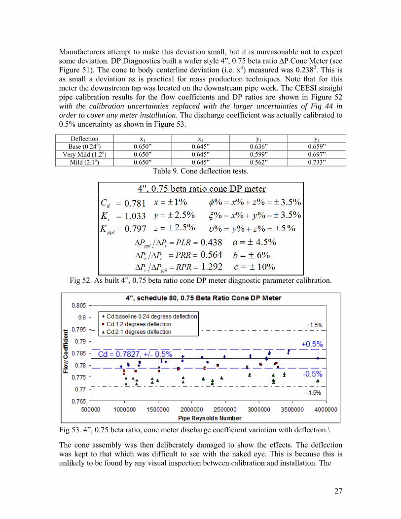
5c. Incorrectly operating ∆P cone meter data – a damaged cone assembly If a non-gusseted cone DP meter is dropped or heavily bumped during transportation or installation, or struck in service by a pressure spike or slug, the shock loading on the cone assembly can cause plastic deformation. Furthermore, a very substantial over speed beyond the design limits can also cause plastic deformation of the cone assembly.
Fig 51. Sketch of a 4”, 0.75 beta ratio cone DP meter.
The design of cone meters has the cone and meter body aligned. In reality manufacturing tolerances mean that the cone usually has a small deviation from the meter centre line.
27
Manufacturers attempt to make this deviation small, but it is unreasonable not to expect some deviation. DP Diagnostics built a wafer style 4”, 0.75 beta ratio ∆P Cone Meter (see Figure 51). The cone to body centerline deviation (i.e. xo) measured was 0.2380. This is as small a deviation as is practical for mass production techniques. Note that for this meter the downstream tap was located on the downstream pipe work. The CEESI straight pipe calibration results for the flow coefficients and DP ratios are shown in Figure 52 with the calibration uncertainties replaced with the larger uncertainties of Fig 44 in order to cover any meter installation. The discharge coefficient was actually calibrated to 0.5% uncertainty as shown in Figure 53.
Fig 52. As built 4”, 0.75 beta ratio cone DP meter diagnostic parameter calibration.
Fig 53. 4”, 0.75 beta ratio, cone meter discharge coefficient variation with deflection.\ The cone assembly was then deliberately damaged to show the effects. The deflection was kept to that which was difficult to see with the naked eye. This is because this is unlikely to be found by any visual inspection between calibration and installation. The
28
Parameter Ranges Pressure Range 13.8 < P (bar) < 31.0
DPt Range 14”WC< DPt <276”WC DPr Range 8”WC <DPr < 156”WC
DPppl Range 6”WC <PPL < 121”WC Reynolds No. Range 946e3 < Re < 6.07e6
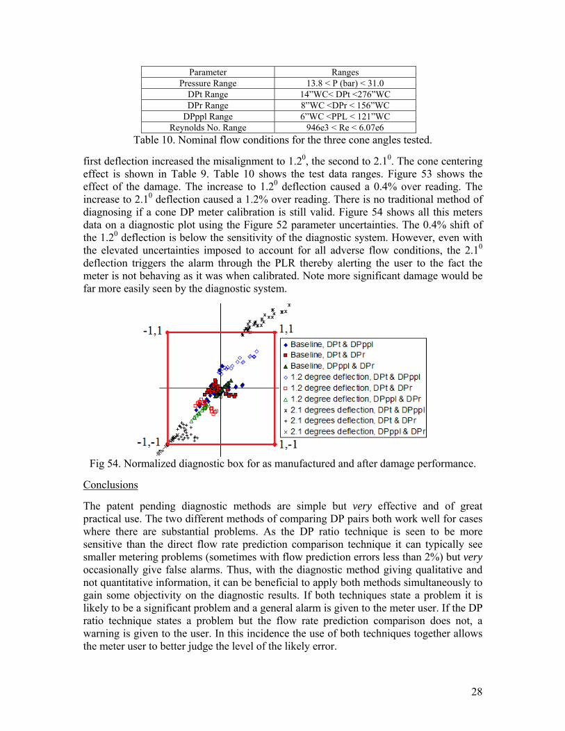
Table 10. Nominal flow conditions for the three cone angles tested. first deflection increased the misalignment to 1.20, the second to 2.10. The cone centering effect is shown in Table 9. Table 10 shows the test data ranges. Figure 53 shows the effect of the damage. The increase to 1.20 deflection caused a 0.4% over reading. The increase to 2.10 deflection caused a 1.2% over reading. There is no traditional method of diagnosing if a cone DP meter calibration is still valid. Figure 54 shows all this meters data on a diagnostic plot using the Figure 52 parameter uncertainties. The 0.4% shift of the 1.20 deflection is below the sensitivity of the diagnostic system. However, even with the elevated uncertainties imposed to account for all adverse flow conditions, the 2.10 deflection triggers the alarm through the PLR thereby alerting the user to the fact the meter is not behaving as it was when calibrated. Note more significant damage would be far more easily seen by the diagnostic system.
Fig 54. Normalized diagnostic box for as manufactured and after damage performance.
Conclusions The patent pending diagnostic methods are simple but very effective and of great practical use. The two different methods of comparing DP pairs both work well for cases where there are substantial problems. As the DP ratio technique is seen to be more sensitive than the direct flow rate prediction comparison technique it can typically see smaller metering problems (sometimes with flow prediction errors less than 2%) but very occasionally give false alarms. Thus, with the diagnostic method giving qualitative and not quantitative information, it can be beneficial to apply both methods simultaneously to gain some objectivity on the diagnostic results. If both techniques state a problem it is likely to be a significant problem and a general alarm is given to the meter user. If the DP ratio technique states a problem but the flow rate prediction comparison does not, a warning is given to the user. In this incidence the use of both techniques together allows the meter user to better judge the level of the likely error.
29
The proposed method of plotting the diagnostic results on a graph with a NDB aids the meter user in this task. Furthermore, although the diagnostics are qualitative and not quantitative, even in this stage of early development certain problems are known to produce a particular signature on the NDB plot thereby indicating what the problem is. Examples are the particular tell tale pattern of points if an orifice plate is installed the wrong way round, or points in the second or fourth quadrant suggest a DP reading problem rather than a meter body problem. As more experience is gained more understanding of the NDB results will be obtained. References 1. Steven, R. “Diagnostic Methodologies for Generic Differential Pressure Flow Meters”, North Sea Flow Measurement Workshop October 2008, St Andrews, Scotland, UK. 2. International Standard Organisation, “Measurement of Fluid Flow by Means of Pressure Differential Devices, Inserted in circular cross section conduits running full”, no. 5167. 3. Johansen, W.R. “Effects of Thin Films of Liquid Coating Orifice Plate Surfaces on Orifice Flowmeter Performance”, Colorado Engineering Experiment Station Inc. report for Gas Research Institution, No. GRI-96/0376. 4. Pritchard M. et al “An Assessment of the Impact of Contamination on Orifice Plate Meter Accuracy”, North Sea Flow Measurement Workshop, St Andrews, Scotland, 2004. 5. Steven, R. “Diagnostic Capabilities of ∆P Cone Meter”, International Symposium of Fluid Flow Measurement 2009, Anchorage, Alaska, USA.