Page 1
PARALLEL BLOCK LANCZOS FOR
SOLVING LARGE BINARY
SYSTEMS
by
MICHAEL PETERSON, B.S.
A THESIS
IN
MATHEMATICS
Submitted to the Graduate Faculty of Texas Tech University in
Partial Fulfillment of the Requirements for
the Degree of
MASTER OF SCIENCE
Approved
Christopher Monico Chairperson of the Committee
Philip Smith
Edward Allen
Accepted
John Borrelli Dean of the Graduate School
August, 2006
Page 2
TABLE OF CONTENTS
ABSTRACT . . . . . . . . . . . . . . . . . . . . . . . . . . . . . . . . . . iii
CHAPTER
I. INTRODUCTION . . . . . . . . . . . . . . . . . . . . . . . . . . . . 1
1.1 Background and Motivation . . . . . . . . . . . . . . . . . . . 1
1.2 Notations . . . . . . . . . . . . . . . . . . . . . . . . . . . . . 3
II. EXISTING METHODS . . . . . . . . . . . . . . . . . . . . . . . . . 4
2.1 Standard Lanczos over R . . . . . . . . . . . . . . . . . . . . . 4
2.2 Montgomery’s Adaptation of Lanczos over F2 . . . . . . . . . 6
2.3 Coppersmith’s Adaptation of Lanczos over F2 . . . . . . . . . 7
III. ALTERNATE METHOD . . . . . . . . . . . . . . . . . . . . . . . . 8
3.1 Gram-Schmidt Lanczos over R . . . . . . . . . . . . . . . . . . 8
3.2 Application over F2 . . . . . . . . . . . . . . . . . . . . . . . . 10
3.3 Constructing the Subspaces . . . . . . . . . . . . . . . . . . . 15
IV. THE ALGORITHM . . . . . . . . . . . . . . . . . . . . . . . . . . . 19
4.1 Summary of the Algorithm . . . . . . . . . . . . . . . . . . . . 19
4.2 Simplifying Expensive Computations . . . . . . . . . . . . . . 20
4.3 Our Adaptation of Lanczos . . . . . . . . . . . . . . . . . . . 22
4.4 Proof of the Algorithm . . . . . . . . . . . . . . . . . . . . . . 24
4.5 Cost of Lanczos . . . . . . . . . . . . . . . . . . . . . . . . . . 27
V. PARALLELIZATION . . . . . . . . . . . . . . . . . . . . . . . . . . 28
5.1 Matrix Storage . . . . . . . . . . . . . . . . . . . . . . . . . . 28
5.2 Operations M and MT . . . . . . . . . . . . . . . . . . . . . . 30
5.3 Two Struct Types . . . . . . . . . . . . . . . . . . . . . . . . 32
5.4 Initialization Code . . . . . . . . . . . . . . . . . . . . . . . . 33
5.5 Master Function . . . . . . . . . . . . . . . . . . . . . . . . . 33
5.6 Slave Functions . . . . . . . . . . . . . . . . . . . . . . . . . . 34
i
Page 3
VI. EFFICIENT IMPLEMENTATION . . . . . . . . . . . . . . . . . . . 35
6.1 Comparing MTM with MMT . . . . . . . . . . . . . . . . . . 35
6.1.1 When A is set to be MTM . . . . . . . . . . . . . . . . 35
6.1.2 When A is set to be MMT . . . . . . . . . . . . . . . . 36
6.2 Computation Tricks . . . . . . . . . . . . . . . . . . . . . . . 38
VII. CONCLUSION . . . . . . . . . . . . . . . . . . . . . . . . . . . . . 41
BIBLIOGRAPHY . . . . . . . . . . . . . . . . . . . . . . . . . . . . . . . 42
ii
Page 4
ABSTRACT
The Lanczos algorithm is very useful in solving a large, sparse linear system Ax =
y and then finding vectors in the kernel of A. Such a system may arise naturally
through number factoring algorithms for example. In this thesis, we present a variant
of the binary Lanczos algorithm that directly finds vectors in the kernel of A without
first solving the system. The number factoring algorithms ultimately require us to
find such vectors. Our adaptation combines ideas of Peter Montgomery and Don
Coppersmith. We also discuss implementation issues, including parallelization.
iii
Page 5
CHAPTER 1
INTRODUCTION
Combining ideas of Peter Montgomery and Don Coppersmith, we wish to develop
a variant of the binary Lanczos algorithm. In Chapter II of this thesis, we describe
briefly the existing methods. In Chapter III, we will describe a geometrically moti-
vated version of the Lanczos algorithm over F2 which will be presented precisely in
the fourth chapter. Finally, we discuss in Chapters V and VI implementation and
efficiency issues followed by a short summary in Chapter VII.
1.1 Background and Motivation
The goal of most Lanczos algorithms is to solve a large system of equations [9].
Such a system can be represented as Ax = y, where A is a large symmetric n × n
matrix. However, if the system is represented by Bx = y, where B is a non-symmetric
matrix, we must somehow obtain a symmetric matrix since this is required by Lanczos.
The standard procedure is to set A = BTB. This construction gives us a symmetric
matrix A. However, it may be preferable in a parallel environment to use A = BBT,
a possibility we will explore later in the thesis.
Large binary linear systems of this type naturally arise from several different
situations. One common way is in factoring numbers using the quadratic sieve [3] or
the general number field sieve (GNFS) [11, 14]. These algorithms produce a sparse
linear system with n on the order of 106 or 107 over F2 which can be represented
as a large, mostly sparse matrix. It follows a very predictable pattern in terms of
where sparse rows and dense rows occur. This will be discussed in detail later in the
parallelization section.
Another place that large binary systems commonly appear is in the linearization
of nonlinear systems over F2 [1, 15]. To attempt to solve a nonlinear system over F2,
an under-determined multivariate system of linear equations is formed by introducing
1
Page 6
new variables to replace nonlinear terms. More equations are obviously needed to be
able to find a solution to the system. After attaining these equations by various
methods, a large matrix A can then represent the system. We now wish to solve
Ax = y for x, which is an ideal candidate for an implementation of the Lanczos
algorithm.
If A is small to moderate in size and invertible, one may compute A−1 explicitly to
solve Ax = y. Even if A is non-invertible, Gaussian elimination can be used to solve
the system, if such solution exists. If A is sparse, we can apply structured Gaussian
elimination [2, 8] to change A into a dense matrix with one-third as many rows and
columns.
However, Gaussian elimination (or structured Gaussian elimination) is a poor
choice in some situations for two reasons: memory and runtime. For example, with
n = 500, 000, a matrix A having .1% nonzero entries would require about 1 GB of
storage if we only store addresses of nonzero entries. For an arbitrary matrix, it would
take about 32 GB to store the entire matrix entry-by-entry. For an invertible n × n
matrix A, Gaussian elimination takes about n3
3additions and the same amount of
multiplications. The matrix A, with n = 500, 000, would require about 8.3 ×10¹⁶
total operations. For a large enough matrix, such as this one, Gaussian elimination
is infeasible because there are too many operations to perform.
Thankfully, Gaussian elimination is not the only way to solve Ax = y. The Lanc-
zos algorithm is also capable of finding the vectors x that solve this, and traditionally
finds such vectors. The methods by Montgomery and Coppersmith solve Ax = y for
vectors x. They let y1 be one such vector. Then Ax = y = Ay1, from which we see
that A(x − y1) = 0. They can find vectors in ker(A) in this fashion. On the other
hand, we do not attempt to solve Ax = y. Our adaptation directly finds vectors in
the kernel of A, i.e.
Ax = 0.
It is likely that our method of finding vectors in the kernel may be modified to also
2
Page 7
solve the linear system problem of Ax = y, although it is not explored further in this
thesis.
Parallelization may allow us to solve much larger problems as we can divide the
work among many machines. The structure of the Block Lanczos algorithm suggests
an efficient parallel implementation. If parallelization allows larger problems to be
solved, then one specific application would be the factorization of larger integers. This
has close ties to cryptography and the security of RSA keys composed of products
of large primes. This algorithm with parallel implementation should facilitate the
factorization of such integers.
1.2 Notations
The following is a short list of notations used through the remainder of the thesis.
• A will denote a symmetric n× n matrix over a field K.
• Ik denotes the k × k identity matrix.
• If V is a k × n matrix, then 〈V 〉 denotes the subspace of Kk generated by the
column vectors of V , i.e. 〈V 〉 = Colsp(V ).
• W is a subspace of Kn.
• Two vectors u and v are defined to be orthogonal if uTv = u · v = 0.
• Two matrices U and V are defined to be orthogonal if each vector u of U is
orthogonal to each vector v of V.
• m represents the index of the last non-zero vector. This means that m + 1 will
be the index of the first zero vector.
3
Page 8
CHAPTER 2
EXISTING METHODS
Peter Montgomery [12] and Don Coppersmith [4] have each given versions of the
Lanczos algorithm over F2 with their own modifications and improvements. Our
eventual goal is to make a slight improvement over these versions. The following is a
broad overview of the widely-used Lanczos method over R and adaptations over F2.
2.1 Standard Lanczos over R
Montgomery gives a description [12] for standard Lanczos over R similar to the
following. Let A be a symmetric n× n matrix over R and y ∈ Rn. To solve Ax = y,
the Lanczos algorithm computes the following sequence of vectors:
w0 = y,
w1 = Aw0 − c1,0w0,
wi = Awi−1 −i−1∑j=0
ci,jwj, (2.1)
where cij =(Awj)
T(Awi−1)
wTj Awj
.
(2.2)
The wi’s are computed until some wi = 0. Let m + 1 denote this first i. For
i < j, by inducting on j and using the symmetry of A, the reader can verify that
wTj Awi = 0 for i 6= j. (2.3)
The proof follows similarly to the end of the proof of Proposition 3.2.3 given later in
Chapter 3. Now we will show that the computation of vectors in the sequence may
be simplified greatly.
Lemma 2.1.1 For the sequence of wj’s above and i < j − 2, cij = 0.
4
Page 9
Proof. From Equations 2.1 and 2.3,
(Awj)T(Awi−1) =
(wj+1 +
j∑k=0
cj+1,kwk
)T
Awi−1
= wTj+1Awi−1 +
j∑k=0
(cj+1,kwk)TAwi−1 = 0.
�
Hence, Equation 2.1 simplifies to
wi = Awi − ci,i−1wi−1 − ci,i−2wi−2 for i ≥ 2. (2.4)
While computing the wi’s, we simultaneously compute
x =m−1∑j=0
wTj y
wTj Awj
wj.
Now, by Equation 2.1,
Ax− y ∈ 〈Aw0, Aw1, . . . , Awm, y〉 ⊆ 〈w0, w1, . . . ,wm〉. (2.5)
By construction, for 0 ≤ j ≤ m− 1, wTj Ax = wT
j y. Hence,
(Ax− y)T(Ax− y) = 0⇒ Ax = y.
We can also see that Proj(Ax− y, wj) = 0, since
Proj(Ax− y, wj) = wj(wTj wj)
−1wTj (Ax− y)
= wj(wTj wj)
−1wTj (A
m−1∑j=0
wTj y
wTj Awj
wj − y)
= 0−wj(wTj wj)
−1wTj y
= 0.
Most authors work around avoiding the problem vectors by embedding F2 into
another field F2n . Now, instead of a given vector having a 12
chance of being self-
orthogonal, it now has a one in 2n chance. The drawback to this embedding is that
computations become much more complex in the larger field. We now look at specifics
of Montgomery’s and Coppersmith’s adaptations over F2.
5
Page 10
2.2 Montgomery’s Adaptation of Lanczos over F2
For a symmetric n × n matrix A over a field K, let wj be as in the previous
section, with wi 6= 0 for 0 ≤ i < m and wm+1 = 0. When K = R, the vectors from
2.4 satisfy the following:
wTi Awi 6= 0 (0 ≤ i < m),
wTj Awi = 0 (i 6= j),
AW ⊆W , where W = 〈w0, w1, · · · , wm〉.
(2.6)
Montgomery defines two vectors to be A-orthogonal if the second condition of 2.6
is met. We may generalize these three conditions to replace vectors wi with sequences
of subspaces. The Block Lanczos algorithm [7] modifies 2.6 to produce a pairwise A-
orthogonal sequence of subspaces {Wi}mi=0 of Kn. Now, instead of the requirement
that no vector can be A-orthogonal to itself, no vector may be A-orthogonal to all of
Wi.
Montgomery defines a subspace W of Rn as A-invertible if has a basis of column
vectors W such that WTAW is invertible [12]. He constructs a sequence of these W
subspaces such that:
Wi is A-invertible,
WTj AWi = 0 (i 6= j) ,
AW ⊆W , where W =W0 +W1 + · · ·+Wm,
(2.7)
in which, Wk represents the subspace of Kn spanned by all of the columns of Wk.
Eventually, with very high probability there will be a Wi that is not A-invertible,
in other words,WTi AWi = 0. The problem with this is that it is necessary to divide by
WTi AWi very often in computing projections for the algorithm. Peter Montgomery
modifies the Lanczos algorithm to produce a sequence of orthogonal A-invertible
subspaces of (F2)n. Each subspace has dimension close to N , the computer word size.
He applies A to N binary vectors at once, using the machine’s bitwise operators.
Comparing with the work required to apply A to one vector, in this way, we will get
6
Page 11
N − 1 applications for free (at the cost of just the one). Our efficiency increases N -
fold. In the process, he corrects a subspaceWi which is not A-invertible by restricting
to a subspace of Wi which does satisfy the conditions in 2.7 (the complement of this
subspace will then be included in Wi+1).
2.3 Coppersmith’s Adaptation of Lanczos over F2
Coppersmith has more of a geometric motivation than Montgomery. His se-
quence of vectors are pairwise orthogonal, instead of being pairwise A-orthogonal.
He appeals to a solution similar to the look-ahead Lanczos method [13], which al-
lows work in F2. Previous authors have embedded F2 ↪→ F2n to work around the
problem of self-orthogonal vectors. This method computes the subspace Wi by using
AWi−2,Wi−1,Wi−2, . . . ,Wi−k where k is associated to the number of self-orthogonal
rows.
There are a few differences between the two authors in correcting subspaces which
do not satisfy the conditions in 2.7. Coppersmith creates a sequence of subspacesRi to
hold any vectors that break the orthogonality condition of each Wi. After separating
off these vectors at each step, the remaining vectors will have all of the necessary
properties. These vectors that he puts into Ri at each step are the problem vectors,
which are the vectors inWi that are orthogonal to all ofWi. We will use these vectors
to help with constructing future Wi’s as they are not only orthogonal to the current
Wi, but also to all previousWi’s by construction. Coppersmith has many more inner
products to compute than Montgomery, making his adaptation less efficient.
The main purpose of Coppersmith’s paper is to introduce a ‘block-version’ of the
Lanczos algorithm [4], which allows 32 matrix-vector operations for the cost of one.
This is commonly referred to as the ‘Block Lanczos algorithm’ and was developed
earlier, but independent of, the block algorithm of Montgomery.
7
Page 12
CHAPTER 3
ALTERNATE METHOD
In this chapter, we first present a geometrically motivated Lanczos variant over R.
We then discuss and solve the difficulties with adapting this algorithm for use over
F2.
3.1 Gram-Schmidt Lanczos over R
For vectors u, v ∈ Rn, we denote the projection of u onto v by
Proj(u; v) =u · vv · v
v.
The goal is to find vectors in the kernel of some symmetric, N ×N matrix A. We
use the Gram-Schmidt process with the initial sequence of vectors A1y, A2y, A3y, . . .
to create the following sequence:
w0 = Ay
w1 = Aw0 − Proj(Aw0; w0)
...
wj+1 = Awj −j∑
i=0
Proj(Awj; wi).
According to our use of the Gram-Schmidt process the collection of vectors
{w0, . . . ,wk} is orthogonal and has the same span as the sequence we started with:
{Ay, A2y, . . . , Aky}. It follows that wm+1 = 0 for some m, so let m + 1 be the least
such positive integer.
Notice also that the sequence spans an A-invariant subspace. That is,
z ∈ span{w0, w1, . . . ,wm} ⇒ Az ∈ span{w0, w1, . . . ,wm}. (3.1)
8
Page 13
The crucial observation is that the computation of wn+1 may be greatly simplified.
Since wi ·wj = 0 for i 6= j, we have for i ≤ n− 2 that
Awn ·wi = wTnATwi = wT
nAwi
= wn ·
(wi+1 +
i∑j=0
Proj(Awi; wj)
)
= wn ·wi+1 +i∑
j=0
wn · Proj(Awi; wj)
= 0 +i∑
j=0
wn · (αjwj) for some αj ∈ R
= 0.
It now follows that for all i ≤ n− 2, Proj(Awn; wi) = 0, so that for each n > 1:
wn+1 = Awn − Proj(Awn; wn)− Proj(Awn; wn−1)
Finally, we set
x =m−1∑i=0
wi · ywi ·wi
wi,
Theorem 3.1.1 Let A be symmetric N ×N and wj’s as before. If Awi =∑
wjvj
for some vj, then
A(Ax + y) = 0.
Proof. First, notice that Ax + y is in the sequence of wj’s by 2.5. Also, by 3.1,
A(Ax + y) must be in the sequence of wj’s since it is A-invariant. Thus, we may
write
A(Ax + y) =∑
wjzj for some zj
9
Page 14
Now, notice
Proj(Ax + y; wj) =m−1∑j=0
wj(wTj wj)
−1wTj (Ax− y)
=m−1∑j=0
wj(wTj wj)
−1wTj
(m−1∑k=0
Proj(y; wi)
)−wj(w
Tj wj)
−1wTj y
=m−1∑j=0
wj(wTj wj)
−1wTj (wj(w
Tj wj)
−1wTj y)−wj(w
Tj wj)
−1wTj y
=m−1∑j=0
wj(wTj wj)
−1wTj y −wj(w
Tj wj)
−1wTj y
= 0.
It is easy to see now that for all j less than m,
Proj(Ax + y; wj) = 0
Ax + y = 0
Ax + y ∈ ker(A)
A(Ax + y) = 0.
�
3.2 Application over F2
We would like to modify the previous algorithm to work over the field F2. The
obvious problem we encounter is that some vectors may be self-orthogonal (exactly
half of the vectors in (F2)N). This problem is detrimental unless dealt with since
we find it necessary to divide by wTj wj many times. Over F2, W has an orthogonal
complement if and only if there does not exist an x ∈ W such that
x ·w = 0, for all w ∈ W .
If such x exists, then it would have to be in the orthogonal complement, since that
consists of every vector that is orthogonal to each vector in W . This leads us to a
10
Page 15
contradiction because x cannot be in both W and the complement of W . Obviously,
since self-orthogonal vectors exist in F2, an orthogonal complement does not always
exist for a given collection of vectors. A randomly chosen subspace has an orthogonal
complement with probability of about 12. An orthogonal complement is precisely what
is needed in order to be able to project onto a subspace in a well-defined way. The
ability to project onto the constructed sequence of subspaces is an essential ingredient
of the Lanczos algorithm. The following is a simple example of a subspace with no
orthogonal complement.
Example 3.2.1 The subspace A ⊂ F32 spanned by the vectors (1, 0, 0)T and (0, 1, 1)T
does not have an orthogonal complement.
The other two vectors in the subspaceA are (1, 1, 1)T and (0, 0, 0)T. There are 23 =
8 distinct vectors in F32. In this case, we can exhaust the possibility of an orthogonal
complement by brute force. None of the remaining vectors ((1, 0, 1)T, (0, 0, 1)T,
(0, 1, 0)T, (1, 1, 0)T) is orthogonal to all of the vectors in A. To see this, we just need
to find one vector in A that yields an inner product of 1 for each remaining vector.
(1, 0, 1)(1, 0, 0)T = 1
(0, 0, 1)(1, 1, 1)T = 1
(0, 1, 0)(1, 1, 1)T = 1
(1, 1, 0)(1, 0, 0)T = 1
Hence, the complement of A is not orthogonal to A. The root problem in this
example is that the vector (0, 1, 1)T is self-orthogonal. The following proposition
describes (1) how to identify subspaces that have an orthogonal complement and (2)
how to project onto these subspaces.
Proposition 3.2.2 Let W be a subspace of FN2 . W has a basis of column vectors
W so that W = Colsp(W ) with WTW invertible if and only if each u ∈ FN2 can
11
Page 16
be uniquely written as u = w + v with w ∈ W and WTv = 0. Furthermore, this
property is independent of the choice of basis for W.
Proof. Let u ∈ FN2 and set
w = W (WTW )−1WTu, and
v = u−w.
Then w ∈ Colsp(W ) =W , u = v + w and
WTv = WTu−WTw
= WTu−WTW (WTW )−1WTu = 0,
so that WTv = 0 as desired.
Let w′ be another vector in Colsp(W ) so that WT(u−w′) = 0. Then w′ = Wα
for some α ∈ FN2 . So we have 0 = WT(u−w′) = WTu−WTWα whence WTWα =
WTu. Since WTW is invertible, it follows that α = (WTW )−1WTu. Left multiplying
both sides by W , we find that
w′ = Wα = W (WTW )−1WTu = w,
giving us the desired uniqueness property. Furthermore, the converse also holds.
Finally, note that if U is another basis of column vectors for W = Colsp(W ) =
Colsp(U), then U = WA for some invertible matrix A. It follows that
UTU = ATWTWA
= AT(WTW )A,
which is invertible, so the result is independent of the choice of basis. �
12
Page 17
The property of a subspace having an orthogonal complement is a necessary and
sufficient condition for projection onto the subspace to be possible. If W has an
orthogonal complement, then we can project onto W . If WTW is invertible, we
define
Proj(U ; W ) := W (WTW )−1WTU. (3.2)
Geometrically speaking, if we can project a vector onto a sequence of orthogonal
subspaces, then we may see the parts of the vector that lie in each. These projections
are a critical part of the Lanczos algorithm. The following proposition describes the
necessary properties of each subspace and forms the basis for our algorithm over F2.
Proposition 3.2.3 Let A be any n×n matrix. Suppose W0, W1, . . . ,Wm is a sequence
of matrices satisfying all of the following properties:
1. Wi is n× ki.
2. WTi Wi is invertible for 0 ≤ i < m.
3. WTi Wj = 0 for i 6= j.
4. 〈W0, W1, . . . ,Wm〉 is A-invariant.
Then rank(W0|W1| . . . |Wm) =∑m
j=0 kj. Furthermore, if Y =∑m
j=0 WjUj for some
Uj, then Y =∑m
j=0 Proj(Y ; Wj). For any Y with AY ∈ 〈W0, W1, . . . ,Wm〉,
X =m∑
i=0
Wi(WTi Wi)
−1WTi Y
is a solution to A(X + Y ) = 0. In other words, X + Y ∈ ker(A).
Proof. To see first that the n ×∑
ki matrix (W0|W1| . . . |Wm) has full rank, notice
that any linear dependence on the columns of this matrix can be expressed as
W0C0 + W1C1 + . . . + Wm−1Cm−1 = 0,
13
Page 18
for some square Cj matrices of dimension kj × kj. It follows from the hypothesis
that for each i, we have
0 = WTi (W0C0 + W1C1 + . . . + WmCm)
= WTi WiCi.
Since WTi Wi is invertible, Ci must be zero, which implies that the columns are
linearly independent, as desired.
Observe now that if Y =∑m
j=0 WjUj, then for each j
Proj(Y ; Wj) = Wj(WTj Wj)
−1WTj Y
=m∑
i=0
Wj(WTj Wj)
−1WTj WiUi
= Wj(WTj Wj)
−1WTj WjUj
= WjUj,
so that∑
Proj(Y ; Wj) = Y , proving the second statement.
Now, for the third statement, set
U = X + Y.
We know that X is in span{W0, . . . ,Wm}. Since the span is A-invariant, AX
must also be in the span. AY ∈ span{W0, . . . ,Wm} by assumption. Therefore,
A(X + Y ) = AU ∈ span{W0, . . . ,Wm}. Next, we wish to show that Proj(A(X +
Y ); Wk) = Proj(AU ; Wk) = 0 for all k. This will lead us to the desired conclusion.
We show that WTk U = 0.
WTk U =
m−1∑j=0
WTk Wj(W
Tj Wj)
−1WTj Y −WT
k Y
= WTk Y −WT
k Y
= 0.
14
Page 19
Now, using the symmetry of A, for each 1 ≤ k ≤ m,
Proj(AU ; Wk) = Wk(WTk Wk)
−1WTk AU
= Wk(WTk Wk)
−1(AWk)TU
= Wk(WTk Wk)
−1
(m∑
i=0
WiVi,j
)T
U
= Wk(WTk Wk)
−1
(m∑
i=0
V Ti,jW
Ti
)U
= Wk(WTk Wk)
−1
(m∑
i=0
V Ti,j(W
Ti U)
)= 0.
Since Proj(AU ; Wk) = 0, it follows from previous argument that AU = 0, hence
U = X + Y ∈ ker(A). �
3.3 Constructing the Subspaces
The difficulty in adapting Lanczos to F2 is precisely the problem of constructing
a sequence of Wj’s satisfying the hypotheses of Proposition 3.2.3. The natural thing
to try would be
W0 = AY,
Wn+1 = AWn −n∑
j=0
Proj(AWn; Wj).
Notice that for j ≤ n− 2,
AWn ·Wi = WTn AWi
= WTn (Wi+1 +
i∑j=0
Proj(AWn; Wj)
= WTn Wi+1 + WT
n
i∑j=0
SjWj for some matrix Sj
= 0.
15
Page 20
This implies that Proj(AWn; Wj) = 0 for j ≤ n − 2, simplifying the recurrence to
two terms. However, even if WTi Wi is invertible for 0 ≤ i ≤ n, there is no guarantee
that WTn+1Wn+1 is invertible. Indeed, WT
n+1Wn+1 is only invertible with about a 50%
chance. As a result, Proj(−; Wn+1) may not be defined. However, with this recursion
as a starting point, we can build a sequence of Wj’s satisfying the hypotheses of
Proposition 3.2.3.
WTW is invertible if and only if there does not exist an x ∈ W such that x ·w = 0
for all w ∈ W . If WTW is not invertible, we attempt to find a basis for such x
vectors and remove it. The remaining vectors will be linearly independent, making
the resulting W satisfy the invertibility condition. If this inner product is invertible,
then we can project onto the subspace in a meaningful way. This inner product
inverse is required in the definition of projection in 3.2. If rank(WTn+1Wn+1) = r and
r < n, we wish to find an r × r submatrix with rank r. We will see by the following
lemma that this submatrix is invertible.
We may find a maximum subspace that we can project onto by finding a maximal
submatrix which is invertible. We claim that this can be found by taking a number
of linearly independent rows of a given symmetric matrix equal to the rank of the
matrix. The following lemma and proof are adapted from Montgomery [12].
Lemma 3.3.1 Let R be a symmetric n× n matrix over a field K with rank r. Upon
selecting any r linearly independent rows of R, the r×r submatrix of R with the same
column indices is invertible.
Proof. After simultaneous row and column permutations, we may assume that
R =
R11 R12
R21 R22
.
where R11 is the symmetric n × n matrix claimed to be invertible. Then R22 is also
symmetric, and R12 = RT21. Note that we just need to show that the matrix R11 has
16
Page 21
rank r (i.e. full rank) to show it is invertible. The first r columns of R are linearly
independent and the rest of the columns are dependent on these, so these first r
columns must generate all of R. This implies that there must exist some r × (n− r)
matrix T such that R11
R21
T =
R12
R22
.
From this we find that
R12 = R11T
R21 = RT12 = TTRT
11 = TTR11
R22 = R21T = RT12T = TTRT
11T = TTR11T.
Now we can substitute for each component of R and rewrite the matrix:
R =
R11 R12
R21 R22
=
R11 R11T
TTR11 TTR11T
=
Ir 0
TT In−r
R11 0
0 0
Ir T
0 In−r
Since the first and last matrices of the final line are invertible (lower triangular and
upper triangular, respectively), rank(R11) = rank(R). Thus, rank(R11) = rank(R) =
r. �
If the specified subspace is not invertible, we need to find and remove a basis
for the “singular part.” Once we remove this, the subspace will be invertible, hence
allowing us to project onto it.
17
Page 22
If W0, . . . ,Wn have been computed, attempt to compute Wn+1 first by setting
E = AWn −n∑
j=0
Proj(AWn; Wj). (3.3)
If E does not have full rank, we can immediately recover some vectors in ker(A).
The vectors which we can recover are vectors x ∈ E such that Ax = 0. If E has full
rank, then we cannot immediately recover any vectors in the kernel of A. According
to Lemma 3.3.1, if rank(ETE) = r, then we can take any r linearly independent rows
of ETE to find the invertible submatrix. If E has full rank but ETE is not invertible,
then let P = [Dn+1|E], where Dn+1 is comprised of columns removed from the previous
iteration, and let T = PTP . Perform row operations on T and corresponding column
operations on P by finding some matrix U such that UT is in reduced row echelon
form. The first columns of PU will satisfy all of the necessary conditions from Lemma
3.2.3, and thus are set to be our desired Wn+1. The remaining columns are orthogonal
to all columns of W and to all previous Wj. These columns comprise Dn+2, which is
used in the next iteration.
We show how to simplify the recurrence later in the proof of the algorithm. We
will see that it can be simplified to a three term recurrence.
18
Page 23
CHAPTER 4
THE ALGORITHM
The following gives an overall description of the algorithm, followed by the al-
gorithm itself, and then the proof that it corrects the problem subspaces that we
encounter along the way.
4.1 Summary of the Algorithm
After initialization, we begin the repeated process of the algorithm. This begins
with setting a matrix E to be A times the previous W . Half the time, this is a two-
term recurrence, and half the time this is a three term recurrence. Next, we look at
the concatenation of the columns of the previous W that were a basis for the vectors
orthogonal to that entire W with this matrix E. Call this concatenation P and set
T = PTP .
We now find some invertible matrix U so that UT is in reduced row echelon form,
causing any zero rows to appear at the bottom. Because
UTUT = U(PTP )UT = (PUT)TPUT
is obviously symmetric, if there are t zero rows at the bottom of UT , there are now
also t zero columns at the right end of UTUT. Also, note that the t zero rows at the
bottom will remain zero rows in UTUT since multiplying on the right by a matrix
UT is just taking linear combinations of columns of UT ; thus, we are performing
simultaneous row and column operations on T .
We may perceive this U matrix as a change of basis since it is finding (1) a basis
for the vectors we may project onto (W ) and (2) a basis for the vectors we cannot
include in this W , i.e. the ones that are orthogonal to each vector in W . We will show
that the upper-left submatrix (everything non-zero) is invertible and has rank equal
to T . Note that the columns of PUT (corresponding to the linear independent rows
of UT ) must be linearly independent and that the remaining rows (corresponding to
19
Page 24
zero rows of UT ) must be dependent on these first rows. The former columns are set
to be W and the latter columns are the ones we will concatenate in the next iteration.
Since the linearly independent rows of UT are the same as the linearly independent
rows of UTUT, we may just work with UT (only necessary to perform row operations
rather than row and column operations). A few tricks and clever observations are
used to get around having to compute some of the expensive matrix inner products.
4.2 Simplifying Expensive Computations
Now, we will describe a clever observation that removes the necessity of one of the
expensive inner products. Fn originally is set to be WTn AWn+1, which would be one of
the inner products we wish to avoid. First, we observe that ETn+1Wn+1 = WT
n AWn+1:
ETn+1Wn+1 = (AWn + WnJnHn + Wn−1Jn−1Fn−1 + Wn−2Jn−2Gn−2)
TWn+1
= (AWn)TWn+1 + (WnJnHn)TWn+1 + (Wn−1Jn−1Fn−1)TWn+1
+ (Wn−2Jn−2Gn−2)TWn+1
= (Wn)TAWn+1 + HTn JT
n WTn Wn+1 + FT
n−1JTn−1W
Tn−1Wn+1
+ GTn−2J
Tn−2W
Tn−2Wn+1
= (Wn)TAWn+1.
Later, in the proof of the algorithm, we see that
(Un+1T )T =
DTn+1Wn+1 DT
n+1Dn+2
ETn+1Wn+1 ET
n+1Dn+2
. (4.1)
Since Fn = WTn AWn+1 = ET
n+1Wn+1, we can avoid computing the inner product and
simply read Fn directly off of (Un+1T )T; it is the lower-left submatrix.
Another expensive vector inner product is Gn, which is originally set to be
WTn−2AWn. We would like to find a shortcut so that we can obtain Gn from something
already computed or something easier to compute (or possibly a combination of both).
20
Page 25
Notice first that
WTn−2AWn = (WT
n AWn−2)T
= (WTn (En−1 −
n−1∑j=0
Proj(AWn−2; Wj)))T
= (WTn (En−1 −
n−1∑j=0
Wj(WTj Wj)
−1WTj AWn−2))
T
= (WTn En−1)
T
= ETn−1Wn.
Also, let kn−1 = dim(Wn−1), and notice that
0 = WTn Wn−1 (4.2)
= WTn [Dn−1|En−1]U
Tn−1Sn−1 (4.3)
= [WTn Dn−1|WT
n En−1]UTn−1Sn−1 (4.4)
where Sn−1 is a matrix that selects the first kn−1 columns from the matrix preceding
it. Taking the transpose, we see that the first kn−1 rows of Un−1
[DT
n−1Wn
ETn−1Wn
]are zero.
Since Un−1 is invertible, ETn−1Wn = 0. Thus, if kn−1 = 64, WT
n−2AWn = ETn−1Wn = 0.
We now proceed to look at the case when kn−1 is not 64. Notice
ETn−1Wn = (WT
n En−1)T
= (WTn [Dn|Wn−1](U
Tn−1)
−1S ′n−2)
T
= ([ WTn Dn| 0 ](UT
n−1)−1S ′
n−2)T
= (S ′n−2)
T(Un−1)−1
[DT
nWn
0
].
Thus, WTn−2AWn is equal to the first kn−2 rows of U−1
n−1
[DT
nWn
0
].
In this algorithm, we make it a requirement that 〈Dn〉 ∈ 〈Wn〉. The following
describes how we will ensure this. Note that we concatenate En+1 to the end of Dn+1.
21
Page 26
We want to find a Un+1 such that
Un+1[Dn+1|En+1]T[Dn+1|En+1] = Un+1
0 DTn+1En+1
ETn+1Dn+1 ET
n+1En+1
is in reduced row echelon form. We must be sure to not zero-out any top rows since
they are from Dn+1 and we must be sure to use all of Dn+1. We begin by looking
for a one in the first column of the above matrix. This one will occur (with high
probability) in one of the first several entries of the ETn+1Dn+1 submatrix since its
entries are fairly random. This ensures us that we will not switch the top row down
to the bottom of the matrix to be cancelled out. We will pivot on this first one and
continue to the second column to find the first one to be that column’s pivot. Since
Dn+1 only consists of a few vectors, we can be sure that they will all be switched into
the early-middle section of the matrix (and thus will not be cancelled out). Therefore,
we can be sure with high probability that 〈Dn+1〉 ∈ 〈Wn+1〉.
4.3 Our Adaptation of Lanczos
Algorithm 4.3.1 F2-Lanczos Kernel
Inputs: a square, symmetric matrix A and a matrix Y
Output: matrix X, which is in the kernel of A
1. Initialize:
n ← −1
W−1 ← Y
k−1 ← 64
All other variables are set to zero.
2. Compute AWn and Hn ← WTn AWn. Set
En+1 ← AWn + WnJnHn + Wn−1Jn−1Fn−1.
22
Page 27
If kn−1 < 64 then do En+1 ← En+1 + Wn−2Jn−2Gn−1.
3. Compute T ← [Dn+1|En+1]T[Dn+1|En+1]. Find an invertible Un+1 so that Un+1T
is in reduced row echelon form. We must carefully find this Un+1 since we make
it a requirement that all of Dn+1 is used in Wn+1 with high probability. We
set kn+1 = rank(T ). Set Wn+1 to be the first kn+1 columns of [Dn+1|En+1]UTn+1
and Dn+2 to be the remaining columns (or zero if there are no columns). If
Wn+1 = 0, then done. Use the fact that
(Un+1T )T =
DTn+1Wn+1 DT
n+1Dn+2
ETn+1Wn+1 ET
n+1Dn+2
, (4.5)
to set Fn ← ETn+1Wn+1 as the lower left kn× kn+1 submatrix. If kn+1 < 64, find
and save U−1n+1. If kn < 64, set Gn ← (the first kn−1 rows of) U−1
n
[DT
n+1Wn+1
0
].
Finally, compute Un+1TUTn+1 and use the fact that
Un+1TUTn+1 =
WTn+1Wn+1 WT
n+1Dn+2
DTn+2Wn+1 DT
n+2Dn+2
, (4.6)
to set Jn+1 ← (WTn+1Wn+1)
−1.
4. Use the fact that Rn, Rn−1, and Rn−2 are known from previous iterations to
compute
DTn+1Y = the last 64− kn rows of Un
[DT
nY
ETn Y
],
ETn+1Y = HT
n JTn (Rn) + (FT
n−1JTn−1)(Rn−1) + (GT
n−2JTn−2)(Rn−2),
Rn+1 = WTn+1Y =
the first kn+1 rows of Un+1
[DT
n+1Y
ETn+1Y
], if n ≥ 0
WT0 Y, if n = −1.
Set X ← X + Wn+1Jn+1(Rn+1).
5. Increment n and go to Step 2.
23
Page 28
4.4 Proof of the Algorithm
We give a proof of our version of the algorithm to show that the assignments are
precise. We also specify why Dn+1 has a high probability of being completely used in
Wn+1 and use this fact to prove the three term recurrence.
First of all, we show that E from Equation 3.3 may be simplified to the three term
recurrence given in the algorithm.
Similar to before, we wish to only subtract off a few projections at each step rather
than the sum of all previous projections. The proof follows similarly to what we have
already done. Notice that for j ≤ n− 2,
AWn ·Wi = WTn AWi
= WTn (Ei+1 +
i∑j=0
Proj(AWn; Wj)
= WTn Ei+1 + WT
n
i∑j=0
WjSj for some matrixSj
= WTn En−1,
which is zero only when Dn−1 = 0, or in other words, En−1 = Wn−1.
However, for i ≤ n− 3,
AWn ·Wi = WTn AWi
= WTn (Ei+1 +
i∑j=0
Proj(AWn; Wj)
= WTn Ei+1 + WT
n
i∑j=0
WjVj for some matrix Vj
= WTn [Wi+1|Di+2](U
T)−1S where S selects the first ki columns.
Now we need to show that WTn Di+2 = 0. The largest index of D is n− 1. Because of
the requirement that 〈Dn−1〉 ⊂ 〈Wn−1〉, and since WTn Wn−1 = 0, we see that WT
n Dn−1
must equal zero. Similarly, this holds true for all i ≤ n− 3 since each D is included
in its respective W and Wn is orthogonal to each of these previous W .
24
Page 29
However, if we try to increase the maximum of i by one, we cannot say that
WTn Dn = 0. Thus, we will have a three term recurrence, so
E = AWn − Proj(AWn; Wn)− Proj(AWn; Wn−1)− Proj(AWn; Wn−2). (4.7)
Only half of the iterations will include the third recurring term. The other half
will only have two recurring terms. Note that in Step 3 if Wn+1 = 0, then we quit
early. This is necessary since later in Step 3 we are required to find (WTn+1Wn+1)
−1.
To prove Equation 4.5, we notice that
(Un+1T )T = (Un+1[Dn+1|En+1]T[Dn+1|En+1])
T
= [Dn+1|En+1]T[Dn+1|En+1]U
Tn+1
= [Dn+1|En+1]T[Wn+1|Dn+2]
=
DTn+1Wn+1 DT
n+1Dn+2
ETn+1Wn+1 ET
n+1Dn+2
,
and for proof of Equation 4.6,
Un+1TUTn+1 = Un+1[Dn+1|En+1]
T[Dn+1|En+1]Un+1
= ([Dn+1|En+1]UTn+1)
T([Dn+1|En+1]Un+1)
= [Wn+1|Dn+2]T[Wn+1|Dn+2]
=
WTn+1Wn+1 WT
n+1Dn+2
DTn+2Wn+1 DT
n+2Dn+2
.
Proposition 4.4.1 Suppose the sequence W0, W1, . . . ,Wn has the same properties as
those in Lemma 3.2.3. Also, suppose DTn [Wn|Dn] = 0. Set
R = U([Dn|E]T[Dn|E]
)for some invertible matrix U such that R is in reduced row echelon form.
Take Wn+1 to be the columns of [Dn|E]UT corresponding to nonzero rows of R,
and take Dn+1 to be the remaining columns – the ones corresponding to the zero rows
of R. Then the following are true.
25
Page 30
1. WTn+1Wn+1 is invertible.
2. DTnWn+1 = 0 and DT
nDn = 0.
Proof. Let r = rank(R). If we select any r linearly independent rows of R, then the
r × r submatrix of R with the same column indices is invertible by Lemma 3.3.1.
R is in reduced row echelon form, so there must be r non-zero rows at the top
of R since r = rank(R). The remaining rows are completely zero and all appear
together at the bottom. Let there be t of these rows. Since U is invertible, we may
right-multiply R by UT.
RUT = U([Dn|E]T[Dn|E]
)UT =
([Dn|E]UT
)T ([Dn|E]UT
)=
WTn+1Wn+1 WT
n+1Dn
DTnWn+1 DT
nDn
Now, we can see that the r × r invertible submatrix WTn+1Wn+1 appears in the
upper-left corner.
Right-multiplying R by a square matrix yields some linear combination of the
columns of R. Thus, the zero rows of R remain zero rows. The matrix RUT will have
t rows of zero at the bottom and t columns of zero together on the right end of the
matrix since RUT is symmetric. Thus,
DTnWn+1 = (DT
nWn+1)T = 0,
and DTnDn = 0.
�
26
Page 31
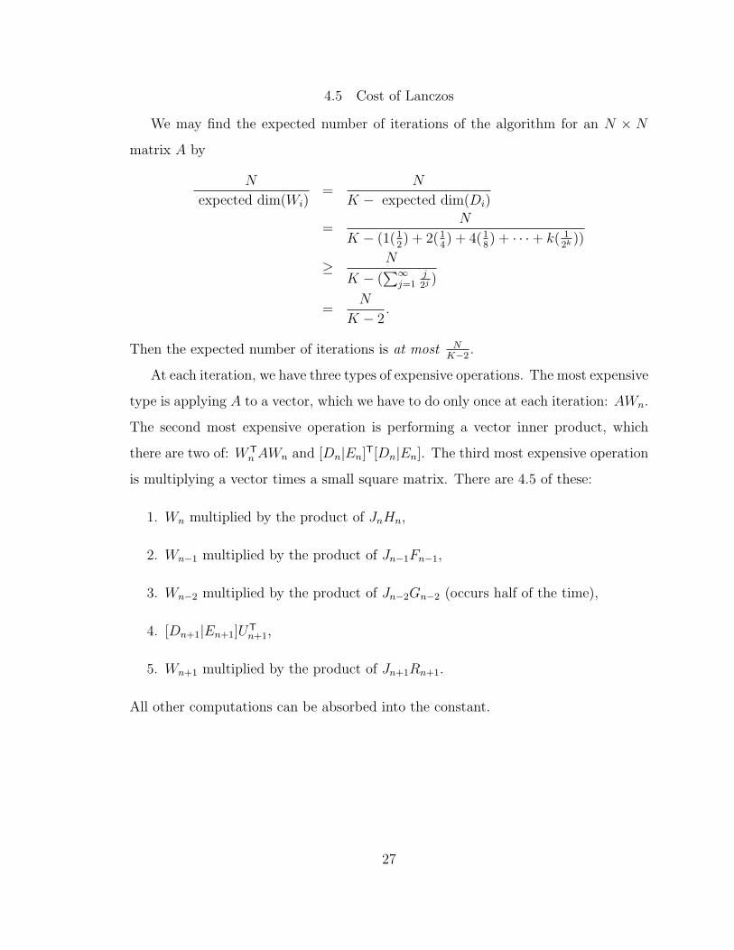
4.5 Cost of Lanczos
We may find the expected number of iterations of the algorithm for an N × N
matrix A by
N
expected dim(Wi)=
N
K − expected dim(Di)
=N
K − (1(12) + 2(1
4) + 4(1
8) + · · ·+ k( 1
2k ))
≥ N
K − (∑∞
j=1j2j )
=N
K − 2.
Then the expected number of iterations is at most NK−2
.
At each iteration, we have three types of expensive operations. The most expensive
type is applying A to a vector, which we have to do only once at each iteration: AWn.
The second most expensive operation is performing a vector inner product, which
there are two of: WTn AWn and [Dn|En]T[Dn|En]. The third most expensive operation
is multiplying a vector times a small square matrix. There are 4.5 of these:
1. Wn multiplied by the product of JnHn,
2. Wn−1 multiplied by the product of Jn−1Fn−1,
3. Wn−2 multiplied by the product of Jn−2Gn−2 (occurs half of the time),
4. [Dn+1|En+1]UTn+1,
5. Wn+1 multiplied by the product of Jn+1Rn+1.
All other computations can be absorbed into the constant.
27
Page 32
CHAPTER 5
PARALLELIZATION
Implementation of the Block Lanczos algorithm is an optimal candidate for par-
allelization. Since the size of the matrix A is so large, the main bottleneck in the
algorithm is the calculation of AX. However, this is easily parallelized by assigning
a different portion of the matrix to each available node, in such a way that the whole
matrix is accounted for. These portions of the matrix are collections of columns
which are multiples of 64 for convenience. The final portion of the matrix obviously
may not have 64 columns exactly; in this case, we may use many different options
such as padding the matrix to give it a complete set of 64 columns. Each slave node
then computes its portion of AX and sends its result back to the master, which will
combine these partial results together to find AX.
First, we discuss the best strategy for storing the matrix. Then we will describe
the parallelization, i.e. initializations and functionality of the master node and slave
nodes.
5.1 Matrix Storage
Recall that the typical matrices which we wish to apply to this algorithm are very
large and mostly sparse. We can take advantage of the latter and store the matrix
in a way that is much more clever than just explicitly storing every entry in the
matrix. Storing each entry is already infeasible for a matrix with n of size 500,000,
since we would need about 32 GB of RAM to store it. Note that this requirement
is much too large to be fulfilled by the RAM of today’s typical machine. Also recall
that our typical n may be two to twenty times larger than this, increasing the RAM
requirement substantially.
First of all, the matrix corresponding to the system of equations that we get
from the number field sieve follows a very predictable pattern. The structure of this
28
Page 33
particular matrix is described to give the reader an excellent example of the Lanczos
algorithm in practice.
The matrix will be stored by collections of rows; each collection may form a dense
block or a sparse block. The number field sieve (much like the quadratic sieve) uses
three factor bases (rational, algebraic, and quadratic characters) in sieving as part of
the process of factoring a large number. Dense rows of the matrix correspond to the
smaller primes, and sparse rows correspond to larger primes. These first few rows
are called dense since they have relatively many nonzero entries. To find the point
where the rows change from dense to sparse, we find the first row with entries having
a probability of less than 164
(assuming 64 is the computer word size) of being a one.
Once this occurs, it will be more worthwhile to store the locations of these entries
rather than storing all the particular entries. This will be the first sparse row, and
hence the first row of our sparse block corresponding to this factor base.
The dense sections of the matrix result from the beginning of the algebraic factor
base, the beginning of the rational factor base, and all of the quadratic character base.
The sparse sections of the matrix result from the remaining parts of the algebraic and
rational factor bases. A typical NFS-produced matrix might look like:
29
Page 34
dense block
sparse block
dense block
sparse block
dense block
where there are far more sparse rows than dense rows.
5.2 Operations M and MT
The GNFS (General Number Field Sieve) has a final step which requires finding
some vectors in the kernel of a matrix M of the form described in the previous section.
The Block Lanczos algorithm is very efficient at finding them. The bottleneck is
computing MX and MTY for the fixed matrix M , and many varying vectors x, y,
etc. Our task is to multiply a matrix M of size r × c by a matrix X of size r × 64
as well as multiplying the transpose of this matrix (i.e. MT) by x. To facilitate this,
assuming we have N -number of processors, we will partition M and x in the following
way:
30
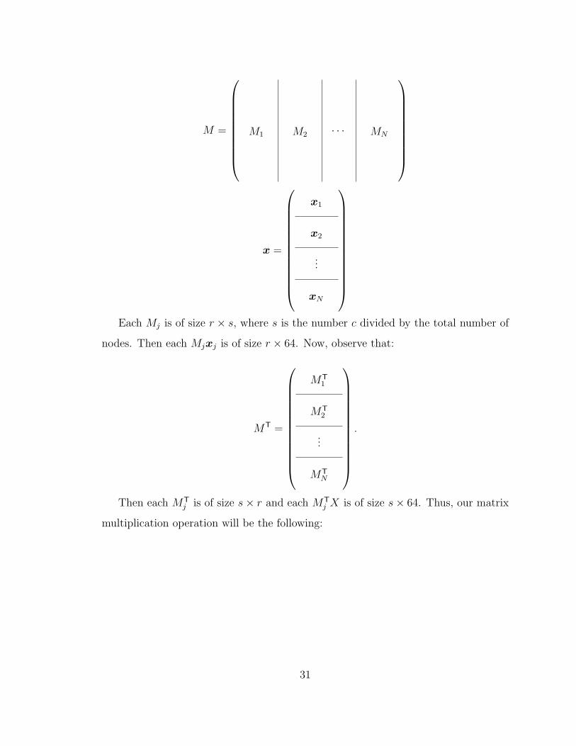
Page 35
M =
M1 M2 · · · MN
x =
x1
x2
...
xN
Each Mj is of size r × s, where s is the number c divided by the total number of
nodes. Then each Mjxj is of size r × 64. Now, observe that:
MT =
MT1
MT2
...
MTN
.
Then each MTj is of size s× r and each MT
j X is of size s× 64. Thus, our matrix
multiplication operation will be the following:
31
Page 36
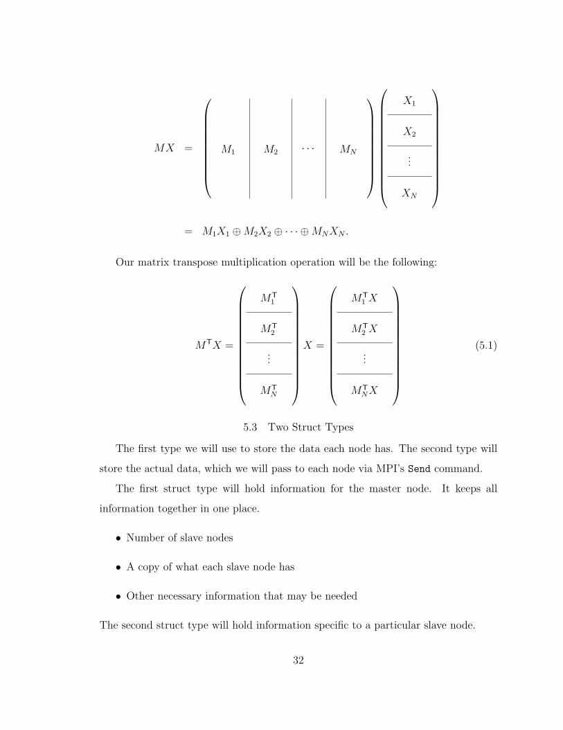
MX =
M1 M2 · · · MN
X1
X2
...
XN
= M1X1 ⊕M2X2 ⊕ · · · ⊕MNXN .
Our matrix transpose multiplication operation will be the following:
MTX =
MT1
MT2
...
MTN
X =
MT1 X
MT2 X
...
MTNX
(5.1)
5.3 Two Struct Types
The first type we will use to store the data each node has. The second type will
store the actual data, which we will pass to each node via MPI’s Send command.
The first struct type will hold information for the master node. It keeps all
information together in one place.
• Number of slave nodes
• A copy of what each slave node has
• Other necessary information that may be needed
The second struct type will hold information specific to a particular slave node.
32
Page 37
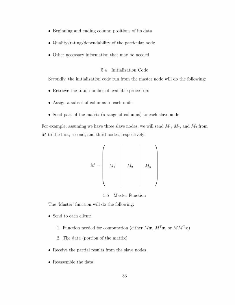
• Beginning and ending column positions of its data
• Quality/rating/dependability of the particular node
• Other necessary information that may be needed
5.4 Initialization Code
Secondly, the initialization code run from the master node will do the following:
• Retrieve the total number of available processors
• Assign a subset of columns to each node
• Send part of the matrix (a range of columns) to each slave node
For example, assuming we have three slave nodes, we will send M1, M2, and M3 from
M to the first, second, and third nodes, respectively:
M =
M1 M2 M3
5.5 Master Function
The ‘Master’ function will do the following:
• Send to each client:
1. Function needed for computation (either Mx, MTx, or MMTx)
2. The data (portion of the matrix)
• Receive the partial results from the slave nodes
• Reassemble the data
33
Page 38
The possible commands (which we will define in the code) are MULT, TMULT, or MMT
to compute Mx, MTx, or MMTx respectively. Each slave node gets its own portion
of the matrix. Reassembling the data at the end is done in one of two ways:
1. Stacking matrices (from TMULT command)
2. Adding the matrices component-wise together via XOR (from MULT or MMT com-
mands)
5.6 Slave Functions
The main loop in the slave functions will do the following:
• Receive the proper command:
1. Function needed for computation (either Mx or MTx)
2. The data x (entire x or a portion xj, depending on the operation)
• Perform the command
• Send the results back to the Master
In the next chapter, we look at ways to improve the parallelization and tricks to
reduce the number of computations.
34
Page 39
CHAPTER 6
EFFICIENT IMPLEMENTATION
There are several ways to make the implementation more efficient. One trick lies
in how we define our square, symmetric matrix A. Other tricks enable us to greatly
decrease our total number of required computations.
6.1 Comparing MTM with MMT
The Lanczos algorithm requires a square symmetric matrix A. The two ways to
find such an A from our given matrix M are
1. A = MTM .
2. A = MMT.
Note that Lanczos never needs the intermediate steps of MTx or Mx. Thus, we are
only interested in finding Ax. We will look closely at each possibility and explain
why MMT is the superior choice.
6.1.1 When A is set to be MTM
Traditionally, A is set to be MTM . Setting A in this way gives a larger square
matrix than MMT yields since M has more columns than rows. Thus, we will have
more total operations to perform using MTM . Another drawback is that our storage
requirements will be greater when dealing with a larger matrix. Also, obviously our
final result Ax will be larger when starting with MTM rather than using MMT.
We will have to use the two commands MULT and TMULT in order to find Ax.
The command MULT, which performs Mx, will be performed first. Assuming we have
three nodes, node 1 will receive the vector x1 (corresponding to section M1 of the
matrix). Node 2 will receive x2 (corresponding to section M2 of the matrix). Node
3 will receive x3 (corresponding to section M3 of the matrix), where x1, x2, and x3
are portions of x in the following way:
35
Page 40
x =
x1
x2
x3
.
Each slave computes its particular result and sends it back to the master. The
master then reassembles the data according to Equation 5.1. By passing to each slave
node only its required part of x, we will avoid sending unnecessary data to each of
the slave nodes. Thus, the bandwidth of information we are sending will be less (than
if we sent the full vector x), which allows for faster results from the slave nodes. In
Equation 5.1, the master adds the results together (each living in mod 2) via XOR
because this is the method of binary addition. This computes the product Mx. Next,
the master sends Mx to each node and the TMULT command. The entire vector
Mx must be sent to each node since each row of MT will need to be multiplied by
the full vector. Note that node j still has its portion Mj of M , so it can just perform
a transpose operation to find MTj . Thus each node does not need any additional data
from M . Each node computes its respective result and sends it back to the master.
The master finally is able to compute MTMx by Equation 5.1, which gives us Ax.
We now show how to recover vectors in the kernel of M given vectors in the kernel
of A. Since 0 = Ax = MTMx, we can see that either x ∈ ker(M) or Mx ∈ ker(MT).
From the latter, we need to make a few observations to find vectors in the kernel
of M . Since M has many more columns than rows, MT has small rank with high
probability. Mx is mostly zero with the nonzero columns being linearly dependent.
We can find linear combinations of the columns to find vectors in ker(M).
6.1.2 When A is set to be MMT
To find MTM we must find the outer product, while finding MMT requires the
inner product. This inner product yields a smaller matrix since A has more columns
36
Page 41
than rows. We would save a lot of bandwidth when sending the blocks of A to the
various nodes. Also, the runtime would be shorter since we require fewer operations
at each step. If A is set to be MMT, we claim that we can cut the number of total
communications in half. Multiplying MMTx, we find that
MMTx =
M1 M2 · · · MN
MT1
MT2
...
MTN
x
=
M1 M2 · · · MN
MT1 x
MT2 x
...
MTNx
= M1M
T1 x⊕M2M
T2 x⊕ · · · ⊕MNMT
Nx.
Thus, each node only needs to receive the full vector x and a portion of the matrix
A. For example, node j will only need to receive x and Mj. It will first find MTj ,
then compute MjMTj x by first applying MT
j to x and then applying Mj to this result.
Note that we do not want to compute and apply MjMTj since it will be much less
sparse than Mj. It will be much more efficient to use MTj and Mj at each step because
of their sparseness. The slave finally sends the result of MjMTj x back to the master.
The master will collect all of these matrices and add them together to find Ax.
This method is much more efficient in terms of bandwidth usage, operations, and
runtime. In the former method, the master had to send to each node twice and receive
from each node twice. In this method, the master only has to send and receive once
37
Page 42
to each node. The number of total communications between master and slave (post
initialization) is exactly one-half of the alternate method. As a side note, we may
save even more communications by using MPI’s Broadcast function, which can send
data to all slave nodes with one command. Also there is no intermediate step for the
master of formulating and resending a new vector.
Now we show how to recover vectors in the kernel of M given vectors in the
kernel of A. Since 0 = Ax = MMTx, we can see that either MTx ∈ ker(M) or
x ∈ ker(MT). The former automatically gives us vectors in ker(M). For the latter,
we need to make a few observations to find vectors in the kernel of M . Since M has
many more columns than rows, MT has small rank with high probability. Certain
linear combinations of these x vectors will yield vectors in ker(M).
However, it could happen that MMT is invertible, in which case we could not set
A = MMT. This problem requires further investigation. An alternate method that
would save the same bandwidth as this description of using MMT would be to use
MTM , but partition by rows (instead of columns as described above). It is difficult to
ensure an even workload to each node because of the distribution of dense and sparse
rows. In general, it appears that setting A = MMT is the best choice (provided
MMT is not invertible).
6.2 Computation Tricks
Coppersmith gives a method ([5] for saving much work in computing the vector
inner products. Say we wish to multiply
V TW =
v1 v2 · · · vn
w1
w2
...
wn
(6.1)
38
Page 43
where V and W are each of size n × k (k much smaller than n). We then make the
following assignments:
Cv1 = w1,
Cv2 = w2,
Cvi= wi.
If any of the vi’s are the same, we add their respective wi values together to get the
value for that Cvi.
Once we have finalized the variables by making a complete pass through V and
W , we will find the solution to V TW with the following. The first row of the solution
matrix will be comprised of the sum of all variables with a one in the first position
of its subscript. The second row will be found by the summation of all variables with
a one in the second position of its subscript. This process continues, and the last
row is found my summing all of the variables with a one in the last position of its
subscript. Note that any variables with subscripts in the given range, for which we
did not encounter a value in V T will be zero. This process can be easily illustrated
with a simple example.
Example 6.2.1 The following inner product can be computed in a way different than
straight matrix multiplication. This method will provide great speedups in runtime
when dealing with inner products such as those we encounter with the Lanczos algo-
rithm.
39
Page 44
Find the inner product of
1 0 1 1 0 1 0
0 0 0 1 1 1 0
1 1 1 0 0 0 0
1 0 1
0 0 1
0 1 0
1 1 1
0 1 1
1 1 0
0 1 1
.
We perform the following assignments/additions in this order:
C5 = C101 = [1 0 1]
C1 = C001 = [0 0 1]
C5 = C101 = C101 + [0 1 0] = [1 1 1]
C6 = C110 = [1 1 1]
C2 = C010 = [0 1 1]
C6 = C110 = C110 + [1 1 0] = [0 0 1]
C0 = C000 = [0 1 1]
The solution matrix P is equal toC100 + C101 + C110 + C111
C010 + C011 + C110 + C111
C001 + C011 + C101 + C111
=
(000) + (111) + (001) + (000)
(011) + (000) + (001) + (000)
(001) + (000) + (111) + (000)
=
1 1 0
0 1 0
1 1 0
.
For this example, the reader may verify with matrix multiplication that this is the
correct product.
He claims that ideas similar to those in the Fast Fourier Transform may be used to
simplify this process. The trick is in finding where to ‘save’ additions since the same
variables are added together in many different places throughout a given computation.
40
Page 45
CHAPTER 7
CONCLUSION
We gave a geometrically motivated version of the Lanczos algorithm. Our adap-
tation shows improvements in computational requirements over Coppersmith. This
algorithm directly finds vectors in the kernel of A without first solving the system. It
is possible that one may find a way to take these vectors in ker(A) and find solutions
to the system Ax = y. Our hope is that this thesis will provide easier comprehension
of the Lanczos algorithm as well as a description for parallel implementation, which
may be used to solve much larger problems.
41
Page 46
BIBLIOGRAPHY
[1] Adams, W. P. and Sherali, H. D. “Linearization strategies for a class of zero-
one mixed integer programming problems”, Operations Research 38 (1990),
217-226.
[2] Bender, E. A. and Canfield, E. R. “An approximate probabilistic model for
structured Gaussian elimination”, Journal of Algorithms 31 (1999), no. 2,
271–290.
[3] Buhler, J. P., Lenstra Jr., H. W., and Pomerance, C., “Factoring integers with
the number field sieve”, The Development of the Number Field Sieve (Berlin)
(A. K. Lenstra and H. W. Lenstra, Jr., eds.), Lecture Notes in Mathematics
1554, Springer-Verlag, Berlin (1993), 50-94.
[4] Coppersmith, D., “Solving linear equations over GF(2): Block Lanczos algo-
rithm”, Linear Algebra Applications 192 (1993), 33–60.
[5] Coppersmith, D., “Solving homogeneous linear equations over GF(2) via block
Wiedemann algorithm”, Mathematics of Computation 62 (1994), no. 205,
333-350.
[6] Coppersmith, D., Odlyzko, A. M., and Schroeppel, R., “Discrete logarithms in
GF(p)”, Algorithmica 1 (1986), 1-15.
[7] Cullum, J. K. and Willoughby, R. A., “Lanczos algorithms for large symmetric
eigenvalue computations”, Vol. I Theory, Birkhauser, Boston, (1985).
[8] Knuth, D. E., “The art of computer programming, volume 2: seminumerical
algorithms”. Addison-Wesley, Reading. Third edition, (1998).
[9] Lanczos, C., “An iterative method for the solution of the eigenvalue problem
of linear differential and integral operators”, Journal of Research National
Bureau of Standards Sec. B 45 (1950), 255-282.
42
Page 47
[10] Lanczos, C., Applied Analysis, Prentice-Hall, Englewood Cliffs, NJ (1956).
[11] Lenstra, A. and Lenstra, H. (eds), “The development of the number field sieve”,
Lecture Notes in Mathematics 1554, Springer-Verlag, Berlin (1993).
[12] Montgomery, P., “A block Lanczos algorithm for finding dependencies over GF
(2)”, Advances in Cryptology - Eurocrypt ’95, Lecture Notes in Computer
Science 921, (1995).
[13] Parlett, B. N., Taylor, D. R., and Liu, Z. A., “A look-ahead Lanczos algorithm
for unsymmetric matrices”, Math. Comp. 44 (1985), 105-124.
[14] Pomerance, C., “The quadratic sieve factoring algorithm”, Advances in Cryptol-
ogy, Proceedings of EUROCRYPT 84 (New York) (T. Beth, N. Cot, and I.
Ingemarsson, eds.), Lecture Notes in Computer Science 209, Springer-Verlag,
169-182.
[15] Van den Bergh, M., “Linearisations of binary and ternary forms”, J. Algebra,
109 (1987), 172-183.
[16] Wiedemann, D. H., “Solving sparse linear equations over finite fields”, IEEE
Trans. Inform. Theory 32 (1986), no. 1, 54-62.
43
Page 48
PERMISSION TO COPY
In presenting this thesis in partial fulfillment of the requirements for a master’s
degree at Texas Tech University or Texas Tech University Health Sciences Center, I
agree that the Library and my major department shall make it freely available for
research purposes. Permission to copy this thesis for scholarly purposes may be granted
by the Director of the Library or my major professor. It is understood that any copying
or publication of this thesis for financial gain shall not be allowed without my further
written permission and that any user may be liable for copyright infringement.
Agree (Permission is granted.)
__________Michael J. Peterson_____________________ __06-29-2006______ Student Signature Date Disagree (Permission is not granted.) _______________________________________________ _________________ Student Signature Date