Parallel Meshing by Enumeratingthe Vertices of the Voronoi cells

Bruno Lévy

ALICE Géométrie & Lumière

CENTRE INRIA Nancy Grand-Est

OVERVIEW

Part 1. Introduction - Motivations

Part 2. Blowing Bubbles: CVT

Part 3. Anisotropy

Part 4. Journey in the 6th dimension

Part 5. The algorithm

Part 6. Results and conclusions

Introduction - Motivations

1

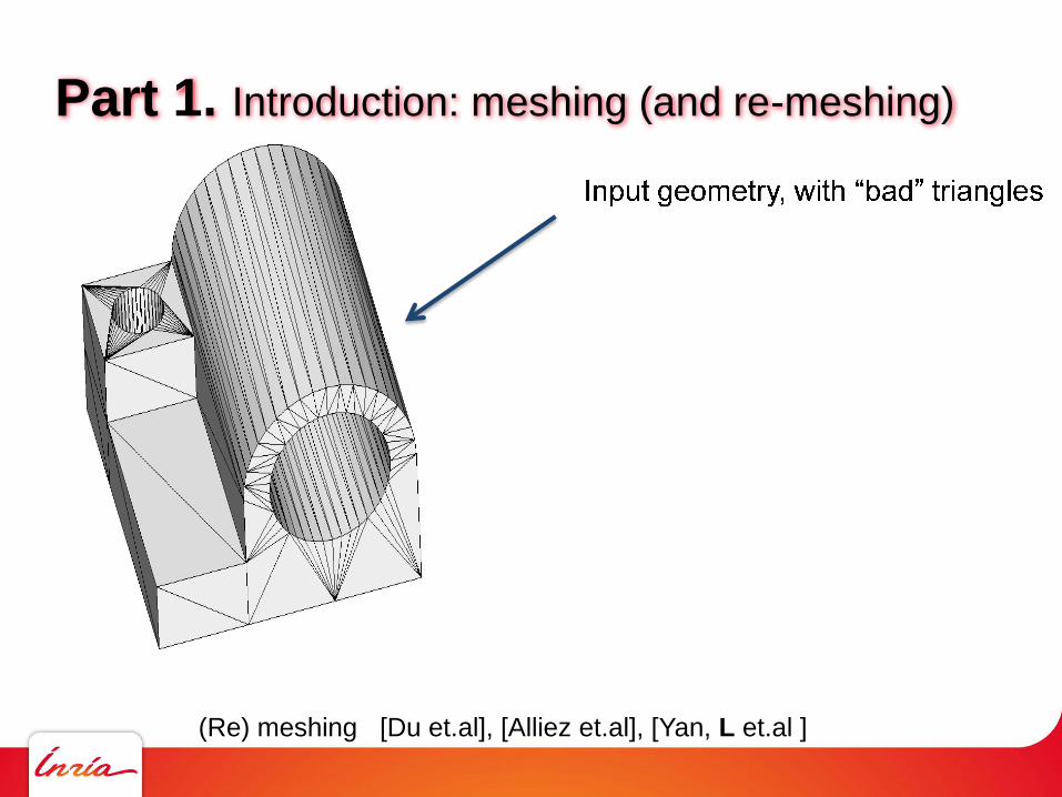
Part 1. Introduction: meshing (and re-meshing)

(Re) meshing [Du et.al], [Alliez et.al], [Yan, L et.al ]

(Re)-meshing [Du et.al], [Alliez et.al], [Yan, L et.al ]

Because extreme angles (near 0o or 180o)

can cause numerical instabilities.

Part 1. Introduction: meshing (and re-meshing)

(Re)-meshing [Du et.al], [Alliez et.al], [Yan, L et.al ]

The result

Part 1. Introduction: meshing (and re-meshing)

Solution-adapted mesh [Miron et.al, Journal of Computational Physics, 2010]

It has skinny triangles where we want

them and oriented as we like (following

the variation of the physics)

Part 1. Introduction: meshing (and re-meshing)

Solution-adapted mesh [Miron et.al, Journal of Computational Physics, 2010]

It has skinny triangles where we want

them and oriented as we like (following

the variation of the physics)

Benefit: higher accuracy with

smaller number of elements.

Part 1. Introduction: meshing (and re-meshing)

Solution-adapted mesh [Miron et.al, Journal of Computational Physics, 2010]

It has skinny triangles where we want

them and oriented as we like (following

the variation of the physics)

Benefit: higher accuracy with

smaller number of elements.

Part 1. Introduction: meshing (and re-meshing)

Skinny triangles:

even sometimes desired but with

controlled shape, size and orientation.

Supersonic flight

[Alauzet et.al]

Part 1. Introduction: meshing (and re-meshing)

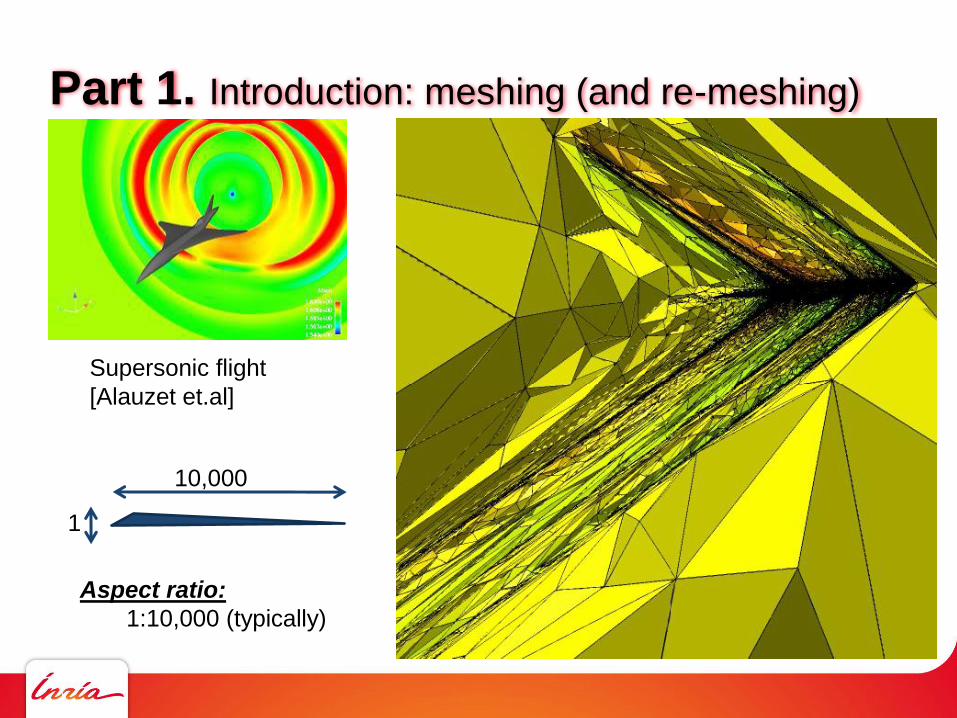
Supersonic flight

[Alauzet et.al]

1

10,000

Aspect ratio:

1:10,000 (typically)

Part 1. Introduction: meshing (and re-meshing)

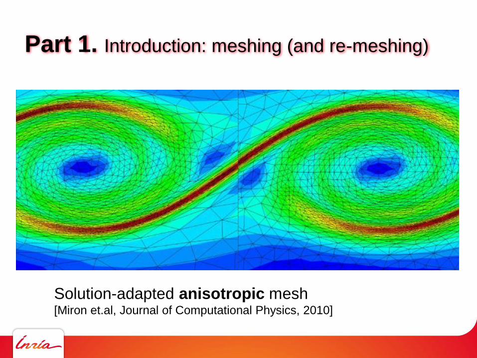
Solution-adapted anisotropic mesh[Miron et.al, Journal of Computational Physics, 2010]

Part 1. Introduction: meshing (and re-meshing)

Part 1. Introduction : mesh classes

Isotropic mesh: All the triangles have

* the same shape (equilateral)

* the same size

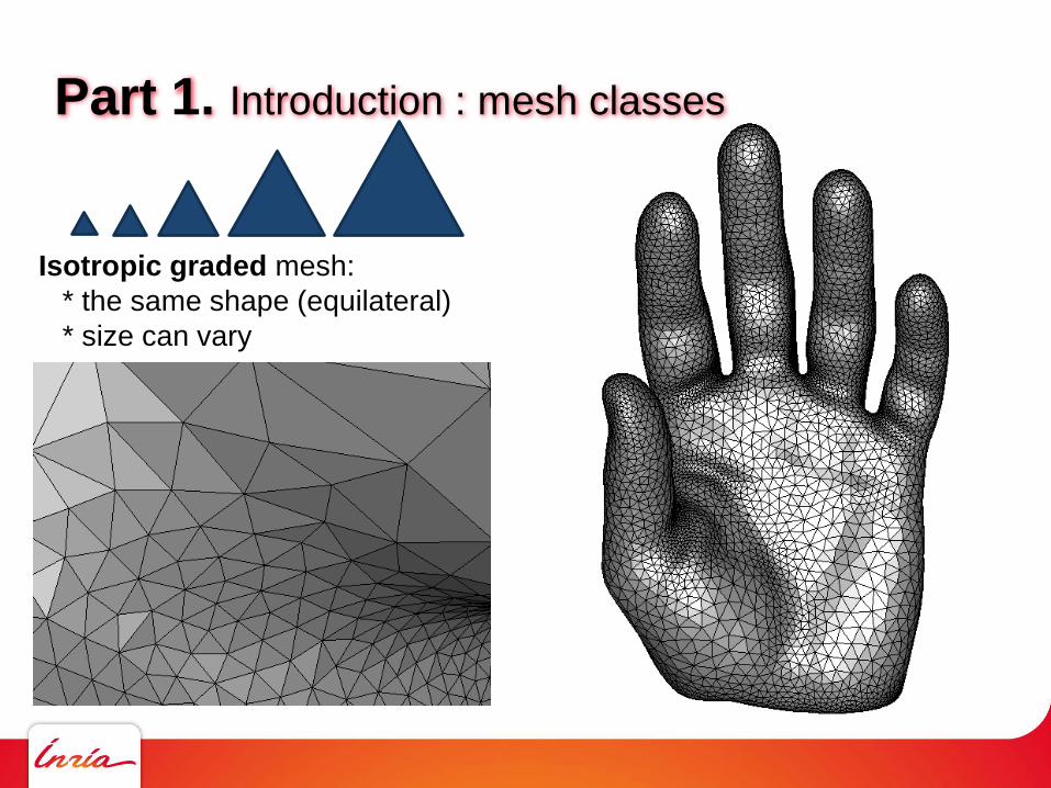
Isotropic graded mesh:

* the same shape (equilateral)

* size can vary

Part 1. Introduction : mesh classes

Anisotropic mesh:

* shape can vary

* size can vary

Part 1. Introduction : mesh classes

Anisotropic mesh:

* shape can vary

* size can vary

Part 1. Introduction : mesh classes

Q: How to

generate an

anisotropic

surface mesh ?

Blowing Bubbles

Centroidal Voronoi Tesselations

2

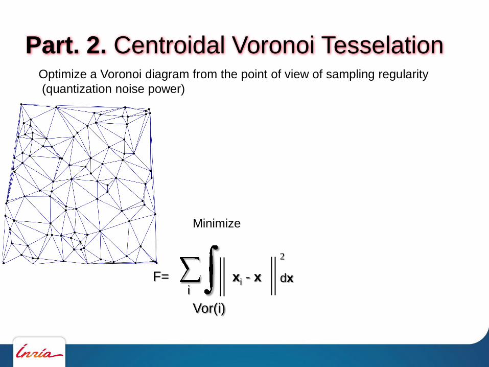
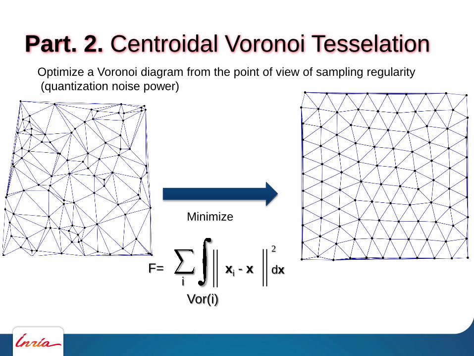
Part. 2. Centroidal Voronoi TesselationOptimize a Voronoi diagram from the point of view of sampling regularity

(quantization noise power)

Optimize a Voronoi diagram from the point of view of sampling regularity

(quantization noise power)

F=

Vor(i)

2

dxxi - xi

Minimize

Part. 2. Centroidal Voronoi Tesselation

Optimize a Voronoi diagram from the point of view of sampling regularity

(quantization noise power)

F=

Vor(i)

2

dxxi - xi

Minimize

Part. 2. Centroidal Voronoi Tesselation

Optimize a Voronoi diagram from the point of view of sampling regularity

(quantization noise power)

F=

Vor(i)

2

dxxi - xi

Minimize

Theorem: F is of class C2 [Liu, Wang, L, Yan, Lu, ACM TOG 2008]

Part. 2. Centroidal Voronoi Tesselation

Part. 2. Centroidal Voronoi Tesselation

Anisotropy

3

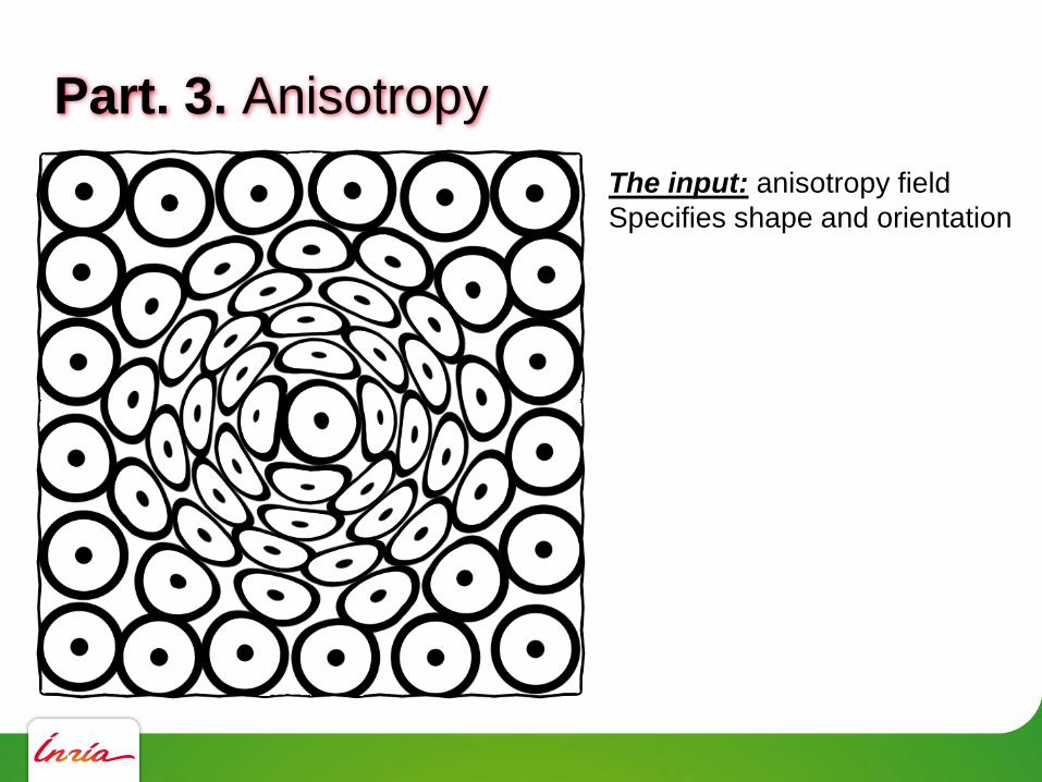
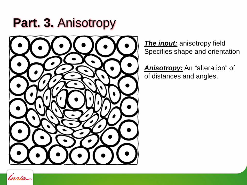
Part. 3. Anisotropy

The input: anisotropy field

Specifies shape and orientation

The input: anisotropy field

Specifies shape and orientation

Anisotropy:

of distances and angles.

Part. 3. Anisotropy

The input: anisotropy field

Specifies shape and orientation

Anisotropy:

of distances and angles.

A point p

Part. 3. Anisotropy

The input: anisotropy field

Specifies shape and orientation

Anisotropy:

of distances and angles.

{ q | dist(p,q) = 1 }

Part. 3. Anisotropy

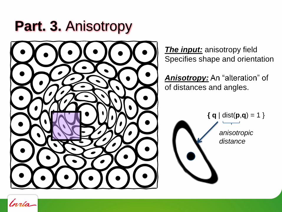
The input: anisotropy field

Specifies shape and orientation

Anisotropy:

of distances and angles.

anisotropic

distance

{ q | dist(p,q) = 1 }

Part. 3. Anisotropy

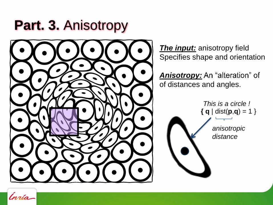
The input: anisotropy field

Specifies shape and orientation

Anisotropy:

of distances and angles.

anisotropic

distance

{ q | dist(p,q) = 1 }This is a circle !

Part. 3. Anisotropy

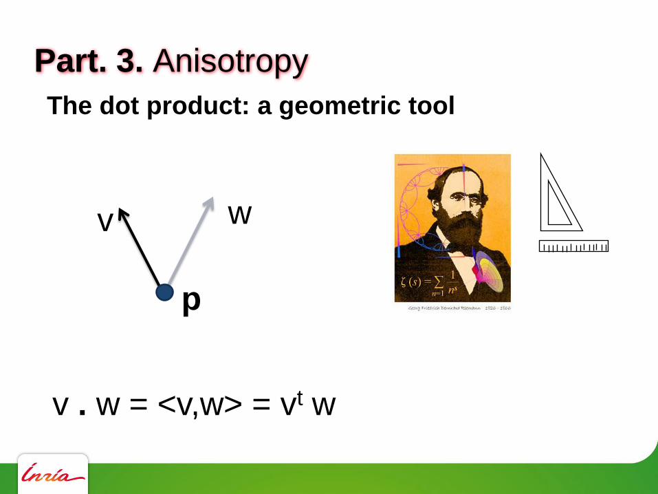
Part. 3. Anisotropy

The dot product: a geometric tool

p

v w

v . w = <v,w> = vt w

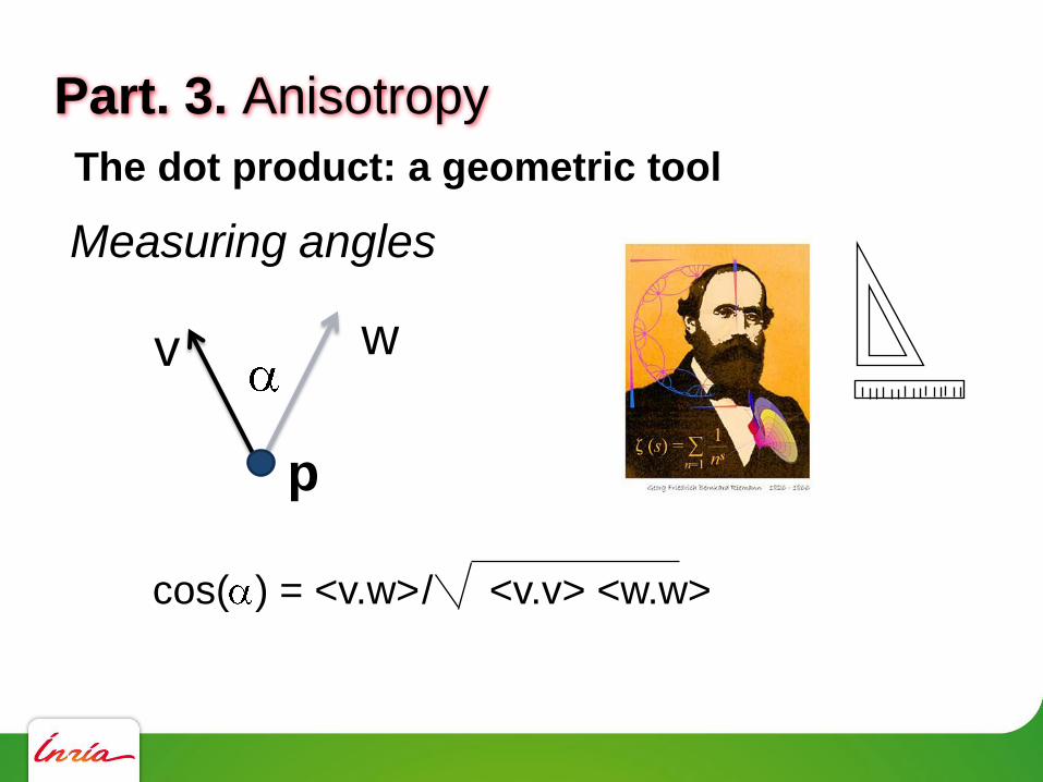
Part. 3. Anisotropy

The dot product: a geometric tool

cos( ) = <v.w>/ <v.v> <w.w>

p

v w

Measuring angles

Part. 3. Anisotropy

The dot product: a geometric tool

||v|| = <v,v>

p

v

Measuring length

Part. 3. Anisotropy

The dot product: a geometric tool

Measuring the length

of a curve

l(C)= ||v(t)|| dt

= <v(t),v(t)> dt t=0

t=1

t=0

t=0

1

1

V(t)

Part. 3. Anisotropy

The dot product: a geometric tool

p

v w

v . w = <v,w> = vt Id w

Changing the dot product

Part. 3. Anisotropy

The dot product: a geometric tool

p

v w

v . w = <v,w> = vt Id w

<v,w>G = vt G(p) w

Changing the dot product

Part. 3. Anisotropy

The dot product: a geometric tool

p

v w

v . w = <v,w> = vt Id w

<v,w>G = vt G(p) wA 2x2 symmetric matrix that depends on p

Changing the dot product

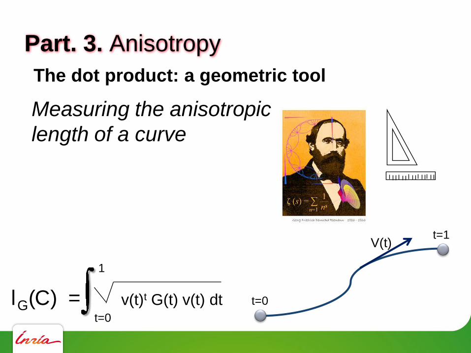
Part. 3. Anisotropy

The dot product: a geometric tool

Measuring the anisotropic

length of a curve

lG(C) = v(t)t G(t) v(t) dt t=0

t=1

t=0

1

V(t)

Part. 3. Anisotropy

The dot product: a geometric tool

Anisotropic distance

between p and q w.r.t. G

lG(C) = v(t)t G(t) v(t) dt p

q

t=0

1

dG(p,q) = (anisotropic) length of

shortest curve

that connects p with q

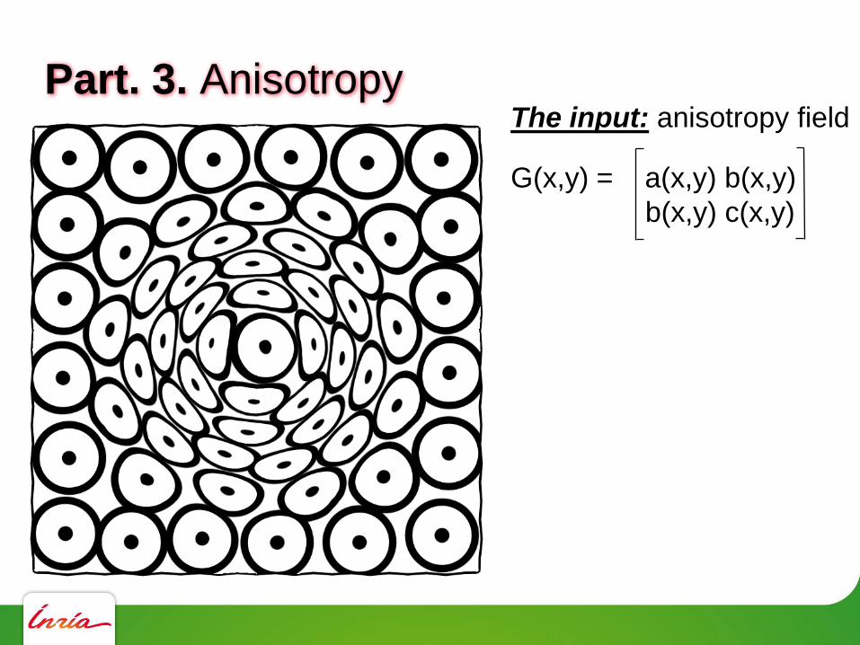
Part. 3. AnisotropyThe input: anisotropy field

G(x,y) = a(x,y) b(x,y)

b(x,y) c(x,y)

Part. 3. Anisotropy

{ q | dG(p,q) = 1 }

p

The input: anisotropy field

G(x,y) = a(x,y) b(x,y)

b(x,y) c(x,y)

The result: triangles are

Part. 3. Anisotropy

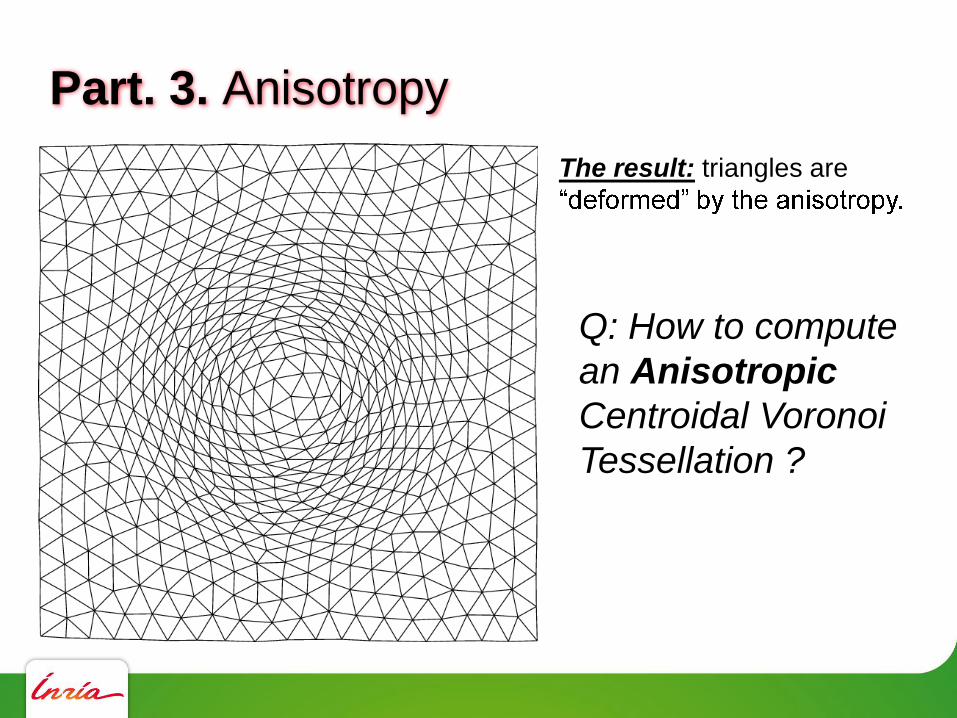
The result: triangles are

Q: How to compute

an Anisotropic

Centroidal Voronoi

Tessellation ?

Part. 3. Anisotropy

Journey in the 6th dimension

beyond

4

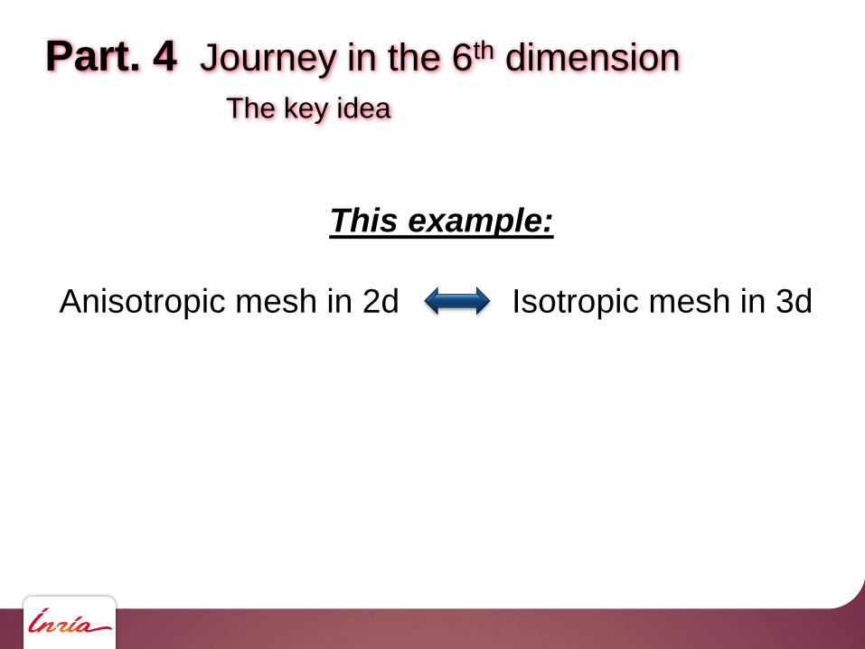
Part. 4 Journey in the 6th dimension

The key idea

This example:

Anisotropic mesh in 2d Isotropic mesh in 3d

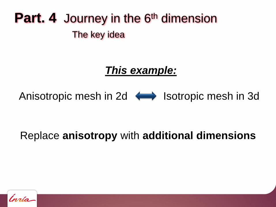
Part. 4 Journey in the 6th dimension

The key idea

This example:

Anisotropic mesh in 2d Isotropic mesh in 3d

Replace anisotropy with additional dimensions

Part. 4 Journey in the 6th dimension

The key idea

Replace anisotropy with additional dimensions

Note: more dimensions may be needed

Part. 4 Journey in the 6th dimension

The key idea

Replace anisotropy with additional dimensions

Note: more dimensions may be needed

How many ?

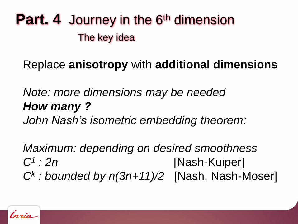
Part. 4 Journey in the 6th dimension

The key idea

Replace anisotropy with additional dimensions

Note: more dimensions may be needed

How many ?

Maximum: depending on desired smoothness

C1 : 2n [Nash-Kuiper]

Ck : bounded by n(3n+11)/2 [Nash, Nash-Moser]

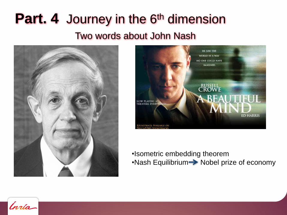
Part. 4 Journey in the 6th dimension

Two words about John Nash

Isometric embedding theorem

Nash Equilibrium Nobel prize of economy

Part. 4 Journey in the 6th dimension

Two words about John Nash

Isometric embedding theorem

Nash Equilibrium Nobel prize of economy

The existence is proved, but it does not tell me how to compute the embedding

given a specified surface and anisotropy field.

Part. 4 Journey in the 6th dimension

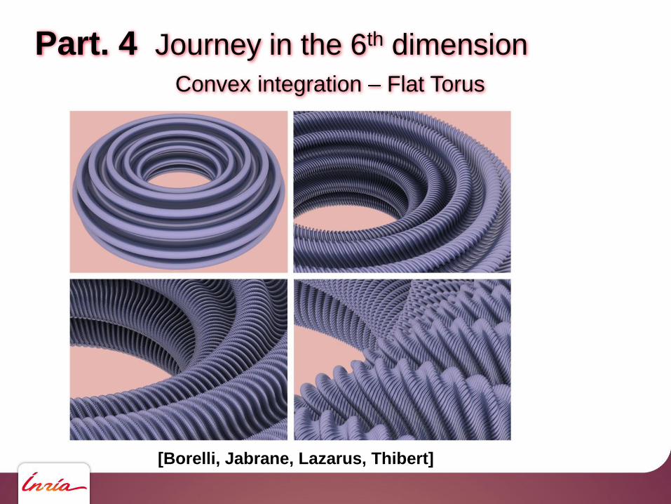
Convex integration Flat Torus

[Borelli, Jabrane, Lazarus, Thibert]

Part. 4 Journey in the 6th dimension

A 6d embedding for curvature-adapted meshing

What we want:

Equilateral triangles

in spherical zones

Part. 4 Journey in the 6th dimension

A 6d embedding for curvature-adapted meshing

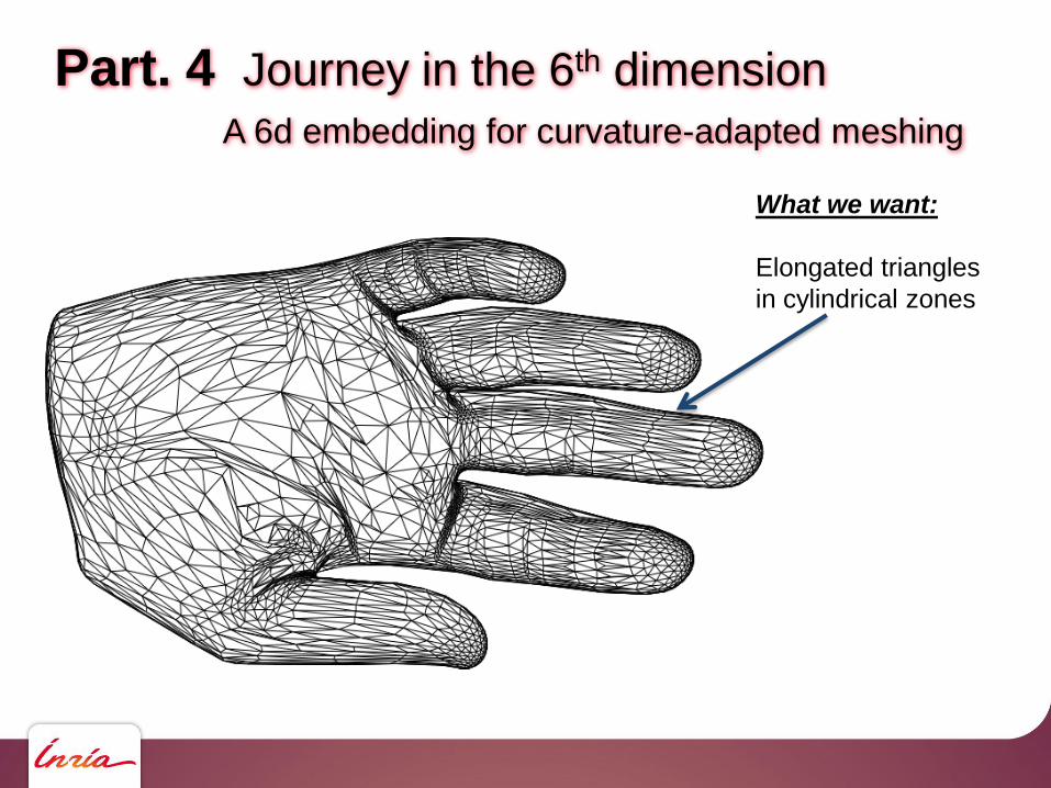
What we want:

Elongated triangles

in cylindrical zones

Part. 4 Journey in the 6th dimension

A 6d embedding for curvature-adapted meshing

The Gauss map:

x

y

z

Nx

Ny

Nz

Part. 4 Journey in the 6th dimension

A 6d embedding for curvature-adapted meshing

The Gauss map:

x

y

z

Nx

Ny

Nz

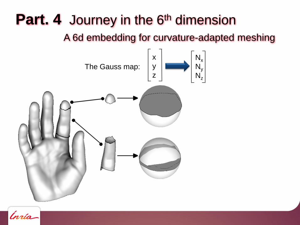
Part. 4 Journey in the 6th dimension

A 6d embedding for curvature-adapted meshing

The Gauss map:

x

y

z

Nx

Ny

Nz

Part. 4 Journey in the 6th dimension

A 6d embedding for curvature-adapted meshing

The Gauss map:

x

y

z

Nx

Ny

Nz

Part. 4 Journey in the 6th dimension

A 6d embedding for curvature-adapted meshing

The Gauss map:

x

y

z

Nx

Ny

Nz

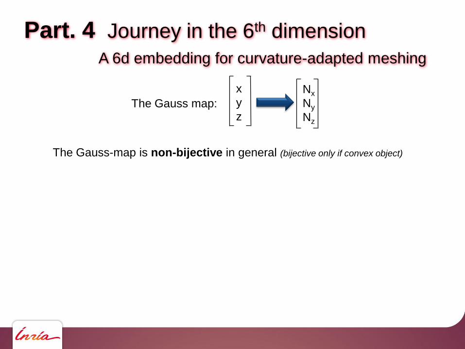
Part. 4 Journey in the 6th dimension

A 6d embedding for curvature-adapted meshing

The Gauss map:

x

y

z

Nx

Ny

Nz

The Gauss-map is non-bijective in general (bijective only if convex object)

Part. 4 Journey in the 6th dimension

A 6d embedding for curvature-adapted meshing

The Gauss map:

x

y

z

Nx

Ny

Nz

The Gauss-map is non-bijective in general (bijective only if convex object)

Our embedding:

x

y

z

x

y

z

sNx

sNy

sNz

Part. 4 Journey in the 6th dimension

A 6d embedding for curvature-adapted meshing

Our embedding:

x

y

z

x

y

z

sNx

sNy

sNzs: desired amount of anisotropy

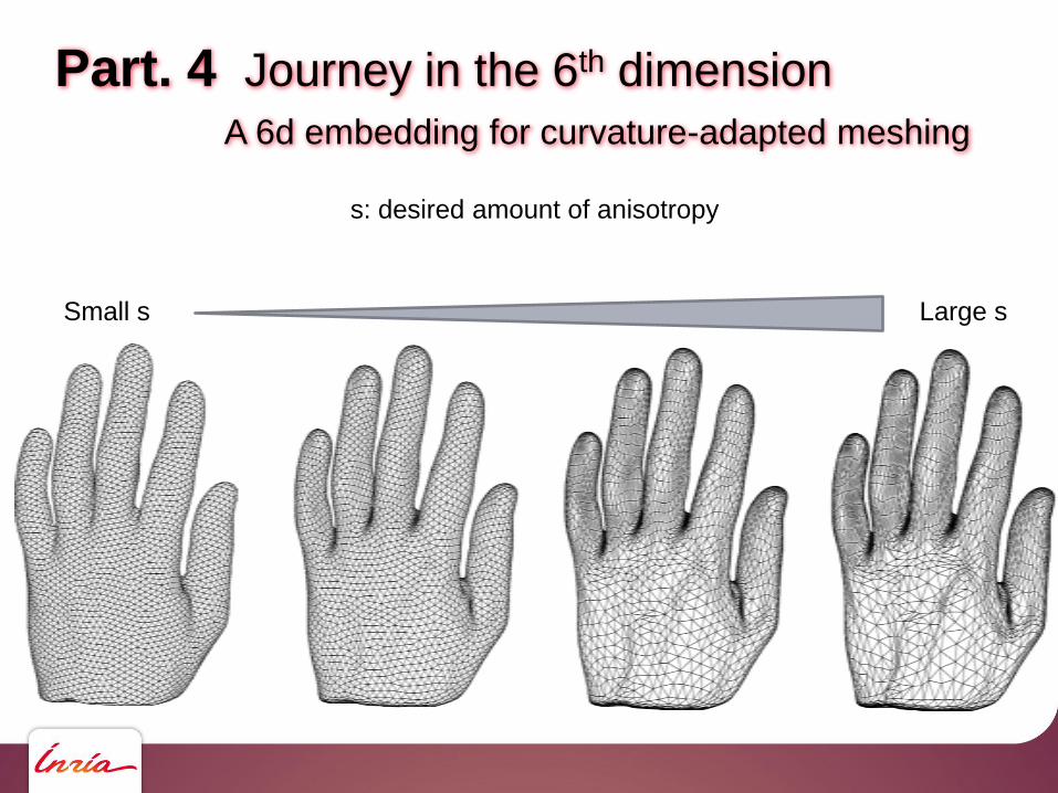
Part. 4 Journey in the 6th dimension

A 6d embedding for curvature-adapted meshing

s: desired amount of anisotropy

Small s Large s

The algorithm

5

Part. 5 The algorithm

(1) Embed the surface S into IR6

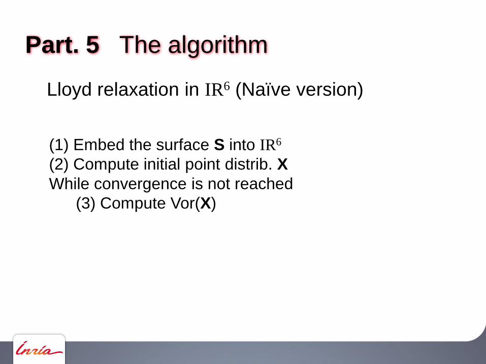
Lloyd relaxation in IR6 (Naïve version)

Part. 5 The algorithm

(1) Embed the surface S into IR6

(2) Compute initial point distrib. X

Lloyd relaxation in IR6 (Naïve version)

Part. 5 The algorithm

(1) Embed the surface S into IR6

(2) Compute initial point distrib. X

While convergence is not reached

Lloyd relaxation in IR6 (Naïve version)

Part. 5 The algorithm

(1) Embed the surface S into IR6

(2) Compute initial point distrib. X

While convergence is not reached

(3) Compute Vor(X)

Lloyd relaxation in IR6 (Naïve version)

Part. 5 The algorithm

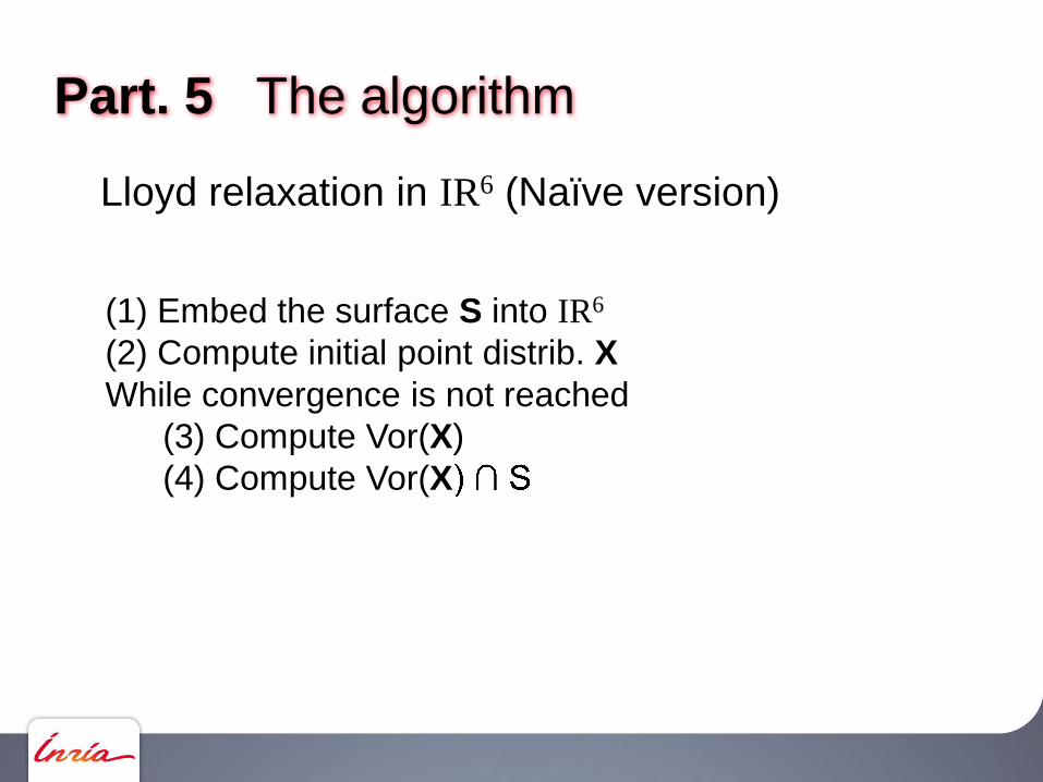
(1) Embed the surface S into IR6

(2) Compute initial point distrib. X

While convergence is not reached

(3) Compute Vor(X)

(4) Compute Vor(X

Lloyd relaxation in IR6 (Naïve version)

Part. 5 The algorithm

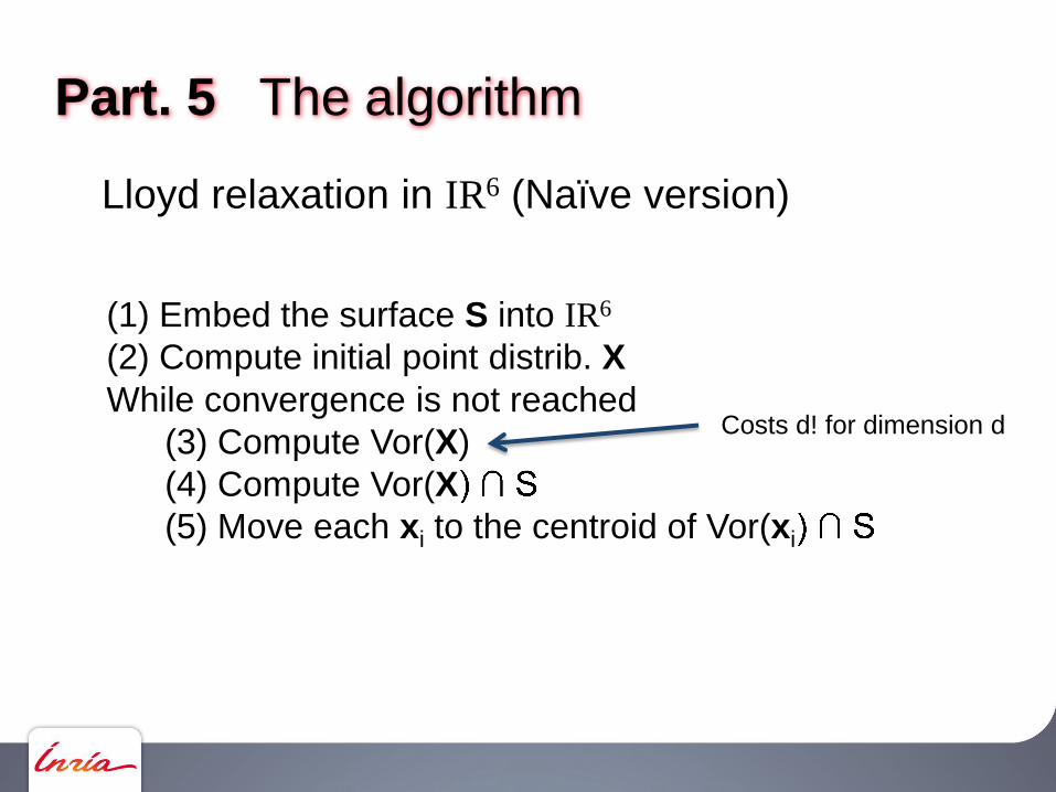
(1) Embed the surface S into IR6

(2) Compute initial point distrib. X

While convergence is not reached

(3) Compute Vor(X)

(4) Compute Vor(X

(5) Move each xi to the centroid of Vor(xi

Lloyd relaxation in IR6 (Naïve version)

Part. 5 The algorithm

(1) Embed the surface S into IR6

(2) Compute initial point distrib. X

While convergence is not reached

(3) Compute Vor(X)

(4) Compute Vor(X

(5) Move each xi to the centroid of Vor(xi

Lloyd relaxation in IR6 (Naïve version)

Costs d! for dimension d

Part. 5 The algorithm

(1) Embed the surface S into IR6

(2) Compute initial point distrib. X

While convergence is not reached

(3) Compute Vor(X)

(4) Compute Vor(X

(5) Move each xi to the centroid of Vor(xi

Lloyd relaxation in IR6 (Naïve version)

Costs d! for dimension d

d = 6 ; d! = 720

Part. 5 The algorithm

(1) Embed the surface S into IR6

(2) Compute initial point distrib. X

While convergence is not reached

(3) Compute Vor(X)

(4) Compute Vor(X

(5) Move each xi to the centroid of Vor(xi

Lloyd relaxation in IR6 (Naïve version)

Curse of dimensionality

Some theoretical results

existence of bounds Tangent Delaunay Complex [Boissonnat et.al.]

Costs d! for dimension d

d = 6 ; d! = 720

Part. 5 The algorithm

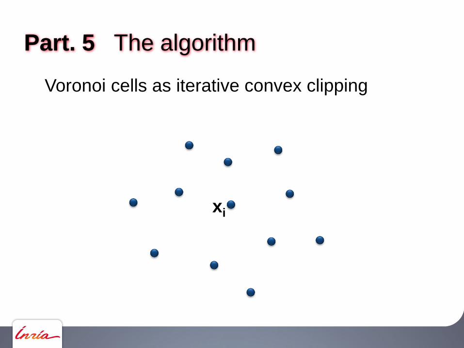
Voronoi cells as iterative convex clipping

xi

Part. 5 The algorithm

Voronoi cells as iterative convex clipping

Neighbors in increasing (6d) distance from xi

xi

x1

x2

x3

x4

x5

x6

x7x8

x9

x10

x11

Part. 5 The algorithm

Voronoi cells as iterative convex clipping

Bisector of xi, x1

xi

x1

x2

x3

x4

x5

x6

x7x8

x9

x10

x11

Part. 5 The algorithm

Voronoi cells as iterative convex clipping

Half-space clipping

xi

x1

x2

x3

x4

x5

x6

x7x8

x9

x10

x11

+(i,1)-(i,1)This side: The other side:

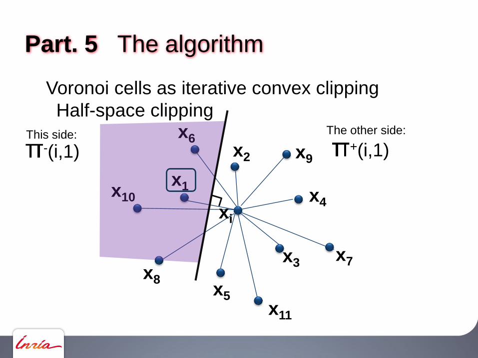
Part. 5 The algorithm

Voronoi cells as iterative convex clipping

Half-space clipping

xi

x1

x2

x3

x4

x5

x6

x7x8

x9

x10

x11

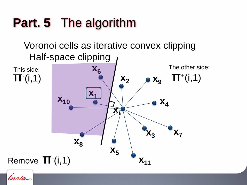
+(i,1)-(i,1)This side: The other side:

Remove -(i,1)

Part. 5 The algorithm

Voronoi cells as iterative convex clipping

Half-space clipping

xi

x1

x2

x3

x4

x5

x6

x7x8

x9

x10

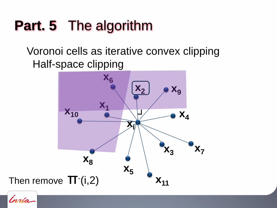
x11Then remove -(i,2)

Part. 5 The algorithm

Voronoi cells as iterative convex clipping

Half-space clipping

xi

x1

x2

x3

x4

x5

x6

x7x8

x9

x10

x11-(i,3)

Part. 5 The algorithm

Voronoi cells as iterative convex clipping

Half-space clipping

xi

x1

x2

x3

x4

x5

x6

x7x8

x9

x10

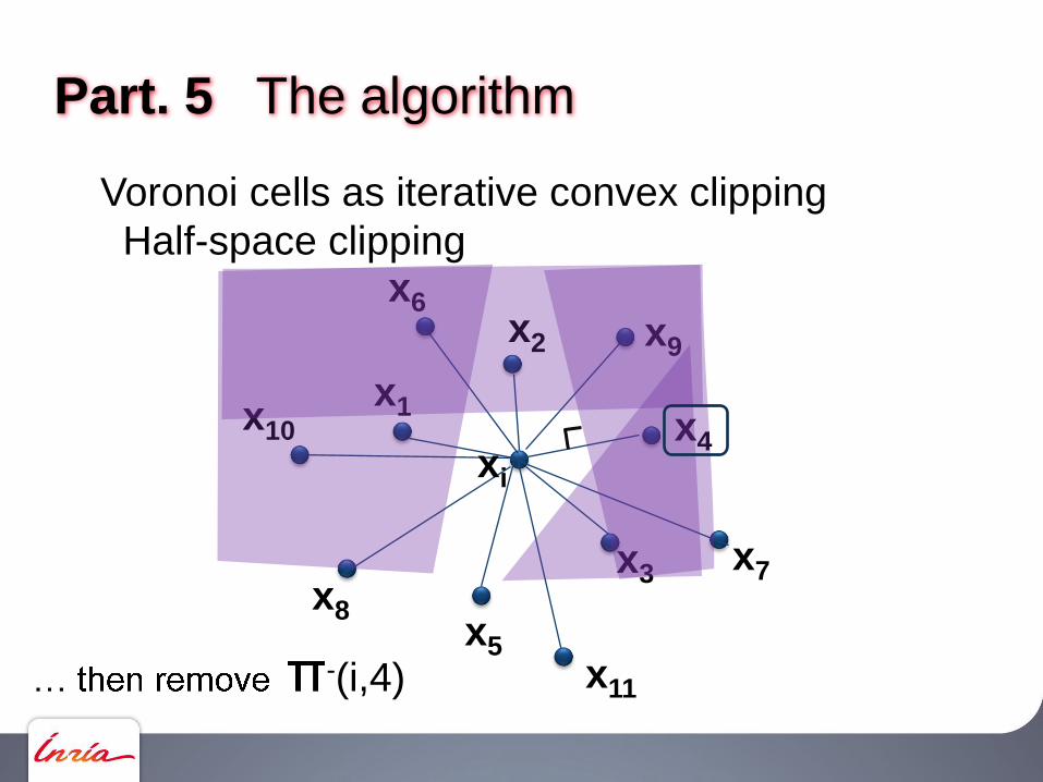
x11-(i,4)

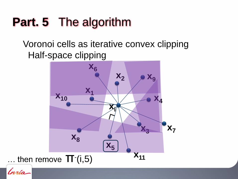
Part. 5 The algorithm

Voronoi cells as iterative convex clipping

Half-space clipping

xi

x1

x2

x3

x4

x5

x6

x7x8

x9

x10

x11-(i,5)

Part. 5 The algorithm

Voronoi cells as iterative convex clipping

When should I stop ?

x1

x2

x3

x4

x5

x7x8

x9

x10

x11

x6

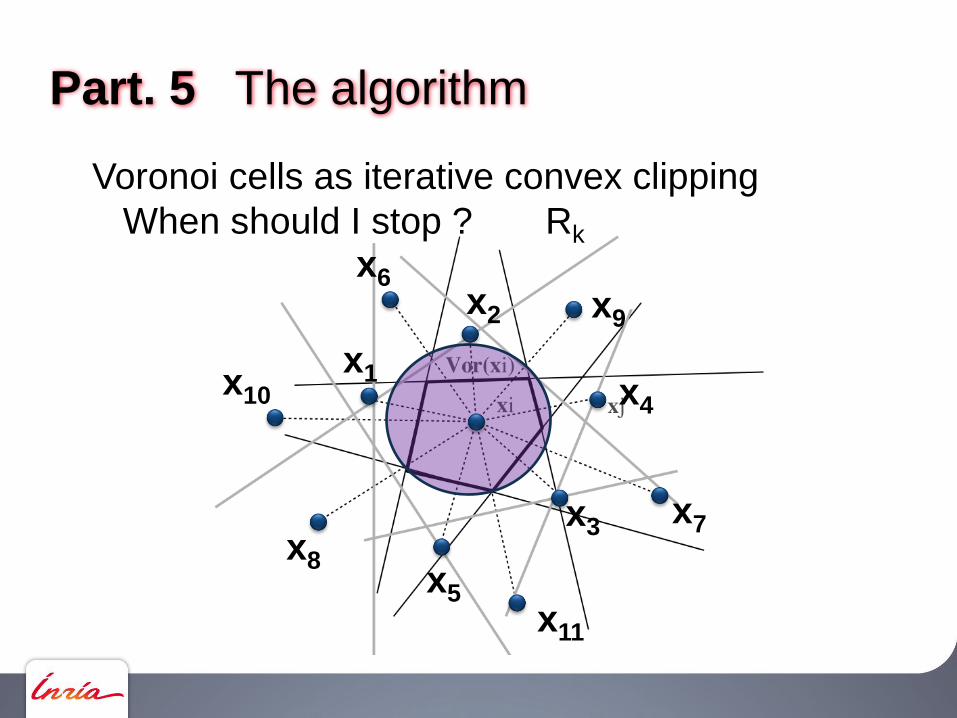
Part. 5 The algorithm

Voronoi cells as iterative convex clipping

When should I stop ? Rk

x1

x2

x3

x4

x5

x7x8

x9

x10

x11

x6

Part. 5 The algorithm

Voronoi cells as iterative convex clipping

When should I stop ?

x1

x2

x3

x4

x5

x7x8

x9

x10

x11

x6

Part. 5 The algorithm

Voronoi cells as iterative convex clipping

When should I stop ? d(xi, xk) > 2 Rk

x1

x2

x3

x4

x5

x7x8

x9

x10

x11

x6

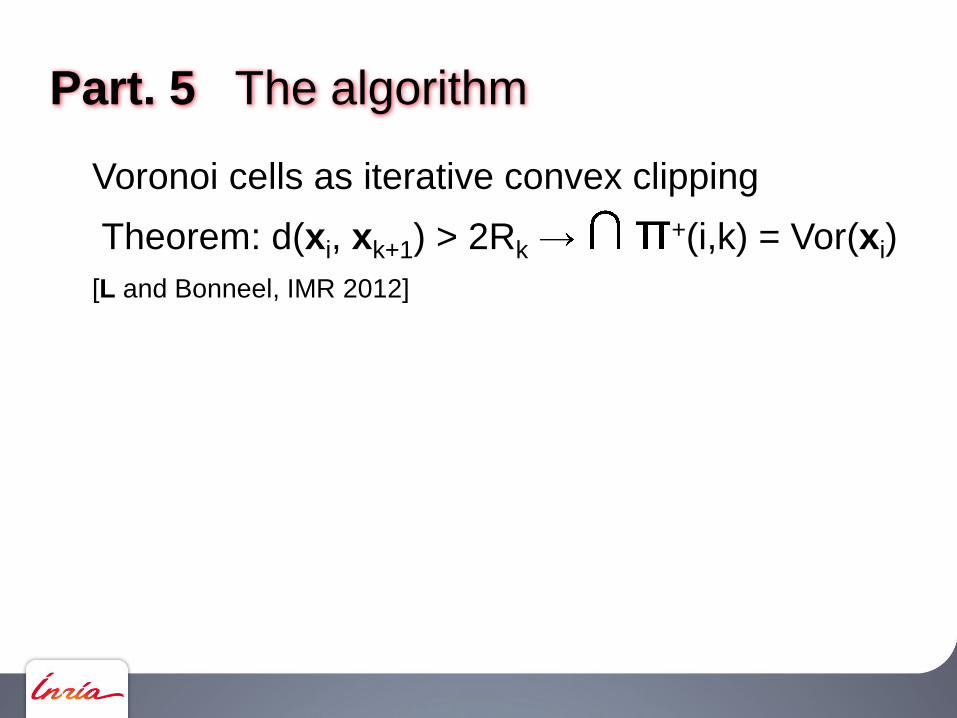
Part. 5 The algorithm

Voronoi cells as iterative convex clipping

Theorem: d(xi, xk+1) > 2Rk+(i,k) = Vor(xi)

[L and Bonneel, IMR 2012]

Part. 5 The algorithm

Voronoi cells as iterative convex clipping

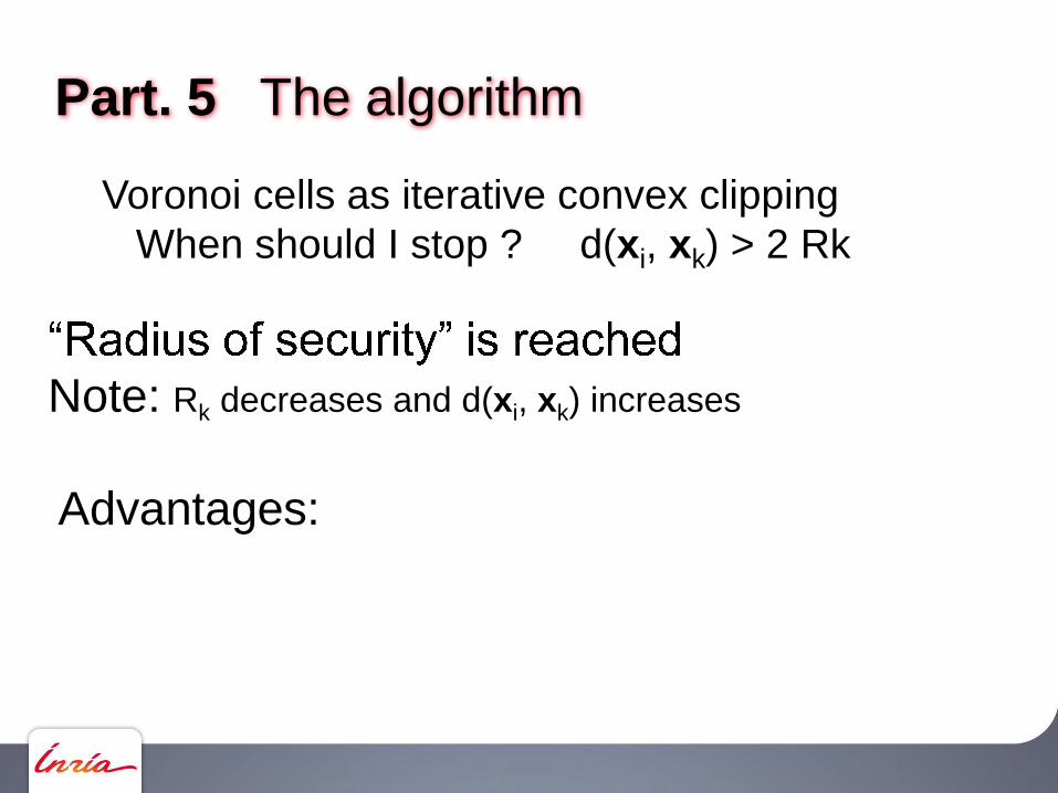
When should I stop ? d(xi, xk) > 2 Rk

Part. 5 The algorithm

Voronoi cells as iterative convex clipping

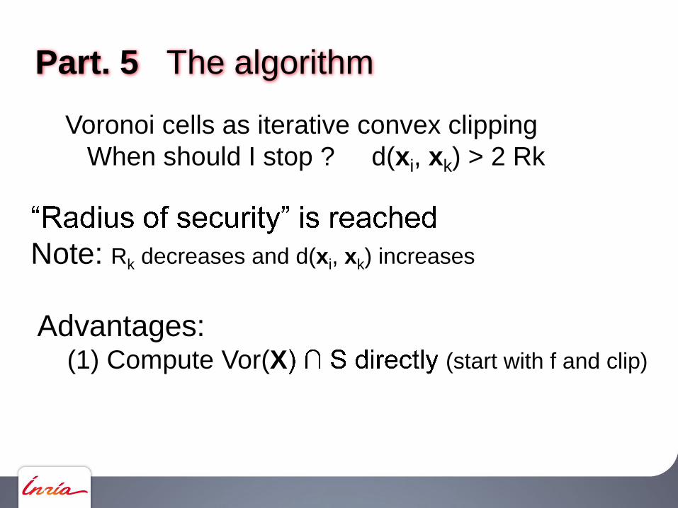
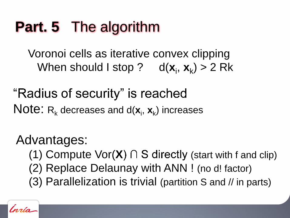
When should I stop ? d(xi, xk) > 2 Rk

Note: Rk decreases and d(xi, xk) increases

Part. 5 The algorithm

Voronoi cells as iterative convex clipping

When should I stop ? d(xi, xk) > 2 Rk

Note: Rk decreases and d(xi, xk) increases

Advantages:

Part. 5 The algorithm

Voronoi cells as iterative convex clipping

When should I stop ? d(xi, xk) > 2 Rk

Note: Rk decreases and d(xi, xk) increases

Advantages: (1) Compute Vor(X (start with f and clip)

Part. 5 The algorithm

Voronoi cells as iterative convex clipping

When should I stop ? d(xi, xk) > 2 Rk

Note: Rk decreases and d(xi, xk) increases

Advantages: (1) Compute Vor(X (start with f and clip)

(2) Replace Delaunay with ANN ! (no d! factor)

Part. 5 The algorithm

Voronoi cells as iterative convex clipping

When should I stop ? d(xi, xk) > 2 Rk

Note: Rk decreases and d(xi, xk) increases

Advantages: (1) Compute Vor(X (start with f and clip)

(2) Replace Delaunay with ANN ! (no d! factor)

(3) Parallelization is trivial (partition S and // in parts)

Some results

6

Part. 6 Some results Filigree (Aim@Shape)

Part. 6 Some results AntEater (Konstanz U.)

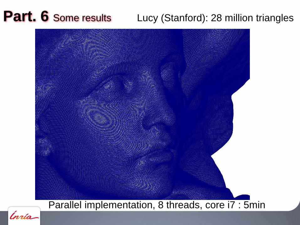
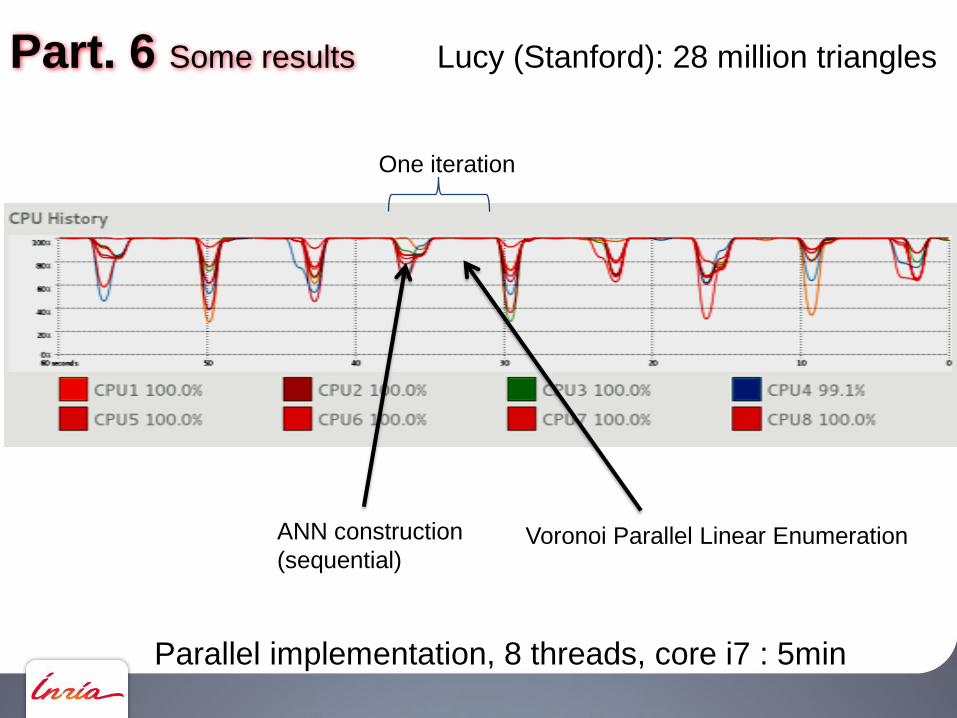
Part. 6 Some results Lucy (Stanford): 28 million triangles

Parallel implementation, 8 threads, core i7 : 5min

Part. 6 Some results Lucy (Stanford): 28 million triangles

Parallel implementation, 8 threads, core i7 : 5min

One iteration

ANN construction

(sequential)Voronoi Parallel Linear Enumeration

Part. 6 Some results Vorpaline mesh, 100K vertices

Part. 6 Some results Porshe (Distene)

Part. 6 Some results Plane (Distene)

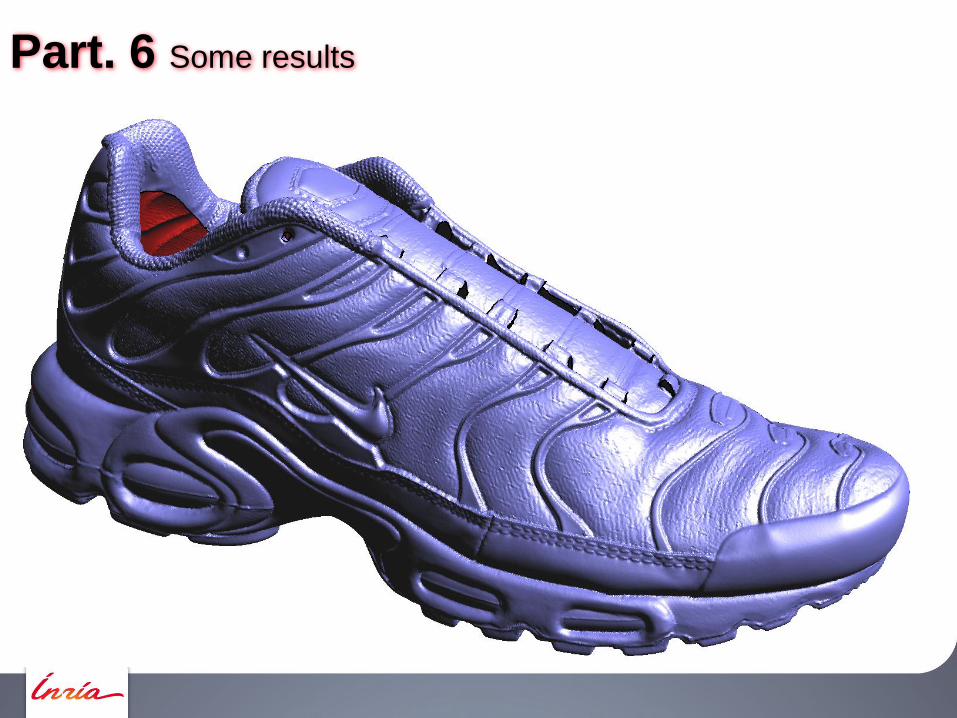
Part. 6 Some results

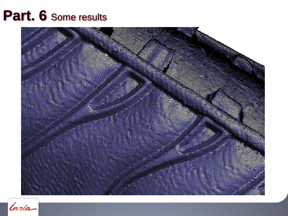
Part. 6 Some results

Part. 6 Some results

Part. 6 What about arbitrary anisotropy ?

Particle-based Anisotropic Surface Meshing[Zhong, Guo, Wang, L, Sun, Liu and Mao, ACM SIGGRAPH 2013]

Part. 6 Reconstruction Co3Ne (Concurrent Co Cone)

Thank you for your attention

Acknowledgements

Wenping Wang (Hong-Kong U.)

Nicolas Bonneel (Harvard U.)

Funding

GOODSHAPE ERC StG 205693

VORPALINE ERC-PoC 334829 pre-industrialization

ANR MORPHO, ANR BECASIM