PARALLEL TETRAHEDRAL MESH REFINEMENT by Mehmet...

PARALLEL TETRAHEDRAL MESH REFINEMENT

by

Mehmet Balman

B.S., Computer Engineering, Bogazici University, 2000

Submitted to the Institute for Graduate Studies in

Science and Engineering in partial fulfillment of

the requirements for the degree of

Master of Science

Graduate Program in Computer Engineering

Bogazici University

2006

ii


APPROVED BY:

Assoc. Prof. Dr. Can Ozturan . . . . . . . . . . . . . . . . . . .

(Thesis Supervisor)

Assist. Prof. Dr. Ali Ecder . . . . . . . . . . . . . . . . . . .

Dr. Ali Vahit Sahiner . . . . . . . . . . . . . . . . . . .

DATE OF APPROVAL: 26.01.2006

iii

ACKNOWLEDGEMENTS

I would like to thank Dr. Can Ozturan for supervising this project. I would also

like to thank Dr. Cem Ersoy for his valuable guidance.

I wish to thank all the people who helped me during this long period. Their

support and encouragement made this work possible.

iv

ABSTRACT


The Adaptive Mesh Refinement is one of the main techniques used for the so-

lution of Partial Differential Equations. Since 3 -dimensional structures are more com-

plex, there are few refinement methods especially for parallel environments. On the

other hand, many algorithms have been proposed for 2 -dimensional structures. We

analyzed the Rivara’s longest-edge bisection algorithm, studied parallelization tech-

niques for the problem, and presented a parallel methodology for the refinement of

non-uniform tetrahedral meshes. The proposed algorithm is practical for real-life ap-

plications and it is also scalable for large mesh structures. We describe a usable data

structure for distributed environments and present a utility using the inter-process

communication. The PTMR utility is capable of distributing the mesh data among

processors and it can accomplish the refinement process within acceptable time limits.

v

OZET

PARALEL DORTYUZLU ORGU IYILESTIRME

Uyarlanmıs Orgu Iyilestirme, Parcalı Turevsel Denklemlerin cozumunde kul-

lanılan ana yontemlerden biridir. Uc boyutlu sistemler daha karmasık oldugundan,

ozellikle paralel ortamlar icin az sayıda arıtma/iyilestirme yontemi mevcuttur. Buna

ragmen iki boyutlu yapılar icin bircok algoritma onerilmistir. Rivara’nın en uzun kenar

bolme teknigi incelenmis, problemin paralel algoritma ile cozumu calısılmıs ve duzensiz

dortyuzlu orguler icin paralel yontem sunulmustur. Onerilen algoritma gercek uygu-

lamalar icin pratik ve buyuk orgu yapıları icin olceklenebilirdir. Dagıtık sistemler

icin kullanılabilir bir veri yapısı anlatılmıs ve islemciler arası haberlesmeyi kullanan

bir uygulama sunulmustur. PTMR uygulaması orgu bilgisini islemcilere dagıtıp kısa

zamanda iyilestirme islemini yapabilmektedir.

vi

TABLE OF CONTENTS

ACKNOWLEDGEMENTS . . . . . . . . . . . . . . . . . . . . . . . . . . . . . iii

ABSTRACT . . . . . . . . . . . . . . . . . . . . . . . . . . . . . . . . . . . . . iv

OZET . . . . . . . . . . . . . . . . . . . . . . . . . . . . . . . . . . . . . . . . . v

LIST OF FIGURES . . . . . . . . . . . . . . . . . . . . . . . . . . . . . . . . . viii

LIST OF SYMBOLS/ABBREVIATIONS . . . . . . . . . . . . . . . . . . . . . xi

1. INTRODUCTION . . . . . . . . . . . . . . . . . . . . . . . . . . . . . . . . 1

1.1. Contributions . . . . . . . . . . . . . . . . . . . . . . . . . . . . . . . . 2

1.2. Outline . . . . . . . . . . . . . . . . . . . . . . . . . . . . . . . . . . . 3

2. MESH REFINEMENT . . . . . . . . . . . . . . . . . . . . . . . . . . . . . . 4

2.1. Refinement of Unstructured Triangulation . . . . . . . . . . . . . . . . 5

2.2. Analysis of the Propagation Path . . . . . . . . . . . . . . . . . . . . . 7

2.3. Skeleton Algorithms . . . . . . . . . . . . . . . . . . . . . . . . . . . . 10

2.4. 8-Tetrahedra Longest Edge (8T-LE ) . . . . . . . . . . . . . . . . . . . 12

2.5. 3-D Sequential Algorithm . . . . . . . . . . . . . . . . . . . . . . . . . 15

3. PARALLEL ALGORITHM . . . . . . . . . . . . . . . . . . . . . . . . . . . 16

3.1. The Longest-Edge Propagation Graph . . . . . . . . . . . . . . . . . . 17

3.2. Longest-Edge Refinement . . . . . . . . . . . . . . . . . . . . . . . . . 18

3.3. 2-D versus 3-D . . . . . . . . . . . . . . . . . . . . . . . . . . . . . . . 20

3.4. Algorithm for Distributed Environments . . . . . . . . . . . . . . . . . 21

4. IMPLEMENTATION DETAILS . . . . . . . . . . . . . . . . . . . . . . . . . 27

4.1. Data Structure . . . . . . . . . . . . . . . . . . . . . . . . . . . . . . . 29

5. TEST RESULTS . . . . . . . . . . . . . . . . . . . . . . . . . . . . . . . . . 34

6. CONCLUSIONS . . . . . . . . . . . . . . . . . . . . . . . . . . . . . . . . . 42

APPENDIX A: PTMR: Reference . . . . . . . . . . . . . . . . . . . . . . . . . 43

A.1. Utilities . . . . . . . . . . . . . . . . . . . . . . . . . . . . . . . . . . . 44

A.1.1. Global Definitions . . . . . . . . . . . . . . . . . . . . . . . . . . 45

A.1.2. Common Utilities . . . . . . . . . . . . . . . . . . . . . . . . . . 46

A.1.3. The Dynamic Pointer Array . . . . . . . . . . . . . . . . . . . . 46

A.1.4. The Pointer Table . . . . . . . . . . . . . . . . . . . . . . . . . 46

vii

A.1.5. Input/Output File Formats . . . . . . . . . . . . . . . . . . . . 47

A.2. Mesh Distribution . . . . . . . . . . . . . . . . . . . . . . . . . . . . . . 49

A.2.1. Processor Ranks . . . . . . . . . . . . . . . . . . . . . . . . . . 49

A.2.2. Processor Mapping . . . . . . . . . . . . . . . . . . . . . . . . . 50

A.2.3. Mesh Partitioning . . . . . . . . . . . . . . . . . . . . . . . . . . 51

A.3. Mesh Operations . . . . . . . . . . . . . . . . . . . . . . . . . . . . . . 55

A.3.1. The Point Object . . . . . . . . . . . . . . . . . . . . . . . . . . 55

A.3.2. The Edge Object . . . . . . . . . . . . . . . . . . . . . . . . . . 57

A.3.3. The Tetrahedron Object . . . . . . . . . . . . . . . . . . . . . . 58

A.3.4. The Tetra Bucket . . . . . . . . . . . . . . . . . . . . . . . . . . 61

A.4. The Refinement Process . . . . . . . . . . . . . . . . . . . . . . . . . . 62

A.4.1. The Structure of a Local Mesh . . . . . . . . . . . . . . . . . . 62

A.5. Communication and the LEPP Synchronization . . . . . . . . . . . . . 66

A.5.1. The Communication Array . . . . . . . . . . . . . . . . . . . . . 66

A.5.2. The LEPP Facility . . . . . . . . . . . . . . . . . . . . . . . . . 68

APPENDIX B: PTMR: Manual . . . . . . . . . . . . . . . . . . . . . . . . . . 70

B.1. Compilation . . . . . . . . . . . . . . . . . . . . . . . . . . . . . . . . . 70

B.2. Libraries . . . . . . . . . . . . . . . . . . . . . . . . . . . . . . . . . . . 73

B.3. Testing . . . . . . . . . . . . . . . . . . . . . . . . . . . . . . . . . . . . 74

B.3.1. Samples . . . . . . . . . . . . . . . . . . . . . . . . . . . . . . . 76

REFERENCES . . . . . . . . . . . . . . . . . . . . . . . . . . . . . . . . . . . . 77

viii

LIST OF FIGURES

Figure 2.1. Longest-Edge Bisection of Triangle t0 . . . . . . . . . . . . . . . . 6

Figure 2.2. Longest-Edge Bisection Algorithm . . . . . . . . . . . . . . . . . . 7

Figure 2.3. Longest-Edge Propagation . . . . . . . . . . . . . . . . . . . . . . 8

Figure 2.4. 4T-LE Refinement . . . . . . . . . . . . . . . . . . . . . . . . . . 8

Figure 2.5. Longest-Edge Propagation Path . . . . . . . . . . . . . . . . . . . 9

Figure 2.6. 2-D Skeleton . . . . . . . . . . . . . . . . . . . . . . . . . . . . . . 11

Figure 2.7. Refinement Patterns of 4-Triangle . . . . . . . . . . . . . . . . . . 12

Figure 2.8. 4-Tetrahedra and 8-Tetrahedra . . . . . . . . . . . . . . . . . . . . 13

Figure 2.9. 3-D Refinement Algorithm . . . . . . . . . . . . . . . . . . . . . . 15

Figure 3.1. LEPP -Graph . . . . . . . . . . . . . . . . . . . . . . . . . . . . . 18

Figure 3.2. 3-D Skeleton Refinement Algorithm . . . . . . . . . . . . . . . . . 19

Figure 3.3. Propagation Path . . . . . . . . . . . . . . . . . . . . . . . . . . . 20

Figure 3.4. Longest-Edge Selection . . . . . . . . . . . . . . . . . . . . . . . . 23

Figure 3.5. Distributed Algorithm . . . . . . . . . . . . . . . . . . . . . . . . 24

Figure 3.6. LEPP -Graph Partitioning and Synchronization . . . . . . . . . . . 25

ix

Figure 3.7. The PTMR Algorithm . . . . . . . . . . . . . . . . . . . . . . . . 26

Figure 4.1. Statistics for the Number of Entities of a Common Mesh . . . . . 30

Figure 4.2. Data Structure of PTMR . . . . . . . . . . . . . . . . . . . . . . . 31

Figure 4.3. Mesh Refinement Example . . . . . . . . . . . . . . . . . . . . . . 31

Figure 4.4. Mesh Refinement Example . . . . . . . . . . . . . . . . . . . . . . 32

Figure 4.5. The Object Relationship of the PTMR Utility . . . . . . . . . . . 33

Figure 5.1. 14904 tetrahedra / 4502 vertices . . . . . . . . . . . . . . . . . . 35

Figure 5.2. 1803 tetrahedra / 527 vertices . . . . . . . . . . . . . . . . . . . . 36

Figure 5.3. 6670 tetrahedra / 2021 vertices . . . . . . . . . . . . . . . . . . . . 37

Figure 5.4. 12586 tetrahedra / 3644 vertices . . . . . . . . . . . . . . . . . . . 37




Figure 5.8. The Refinement Process According to the LEPP Algorithm (elapsed

time spent in the gateway node) . . . . . . . . . . . . . . . . . . . 40

Figure 5.9. The Refinement Process According to the LEPP Algorithm . . . . 40

Figure 5.10. Overall Time . . . . . . . . . . . . . . . . . . . . . . . . . . . . . . 41

x

Figure A.1. The Distributed CSR Format . . . . . . . . . . . . . . . . . . . . . 51

Figure A.2. The Communication Array . . . . . . . . . . . . . . . . . . . . . . 67

xi

LIST OF SYMBOLS/ABBREVIATIONS

α angle

e edge

Einvolved list of selected edges

⊺ tetrahedron

f face

LEPP (t) longest-edge propagation path for triangle t

M1(t) sum of the lengths of longest-edge propagation paths for tri-

angle t

M2(t) the maximum length of longest-edge propagation paths for

triangle t

t triangle

T triangular mesh

τ tetrahedral mesh

v vertex

1-D 1-dimensional

2-D 2-dimensional

3-D 3-dimensional

8T-LE 8-Tetrahedron Longest-Edge

4T-LE 4-Triangle Longest-Edge

AMR Adaptive Mesh Refinement

DAG Directed-Acyclic Graph

LE Longest-Edge

LEPP Longest-Edge Propagation Path

MPI Message Passing Interface

PDE Partial Differential Equation

PTMR Parallel Tetrahedral Mesh Refinement

1

1. INTRODUCTION

Adaptive Mesh Refinement (AMR) is a technique used to effectively solve numer-

ical systems of Partial Differential Equations (PDE ). Instead of processing the uniform

mesh in which grid points are evenly spaced, we place more grid points to the areas

where local error is large in the solution. The adaptive mesh refinement is the pre-

ferred methodology in terms of computational and storage requirements. Refinement

algorithms begin with an initial mesh conforming to a particular geometry, and the

conformity of the overall structure must be preserved after partitioning an element

[1, 2]. Most of the research have focused on mesh components as line segments in

1 -dimension, triangles in 2 -dimension, and tetrahedra in 3-dimension [3, 4].

The triangle refinement process have been studied briefly in recent studies [5, 6, 7].

Since we cannot analyze the elements in a planar view, 3 -dimensional structures yield

to complexities and difficulties. Refining using the skeleton structure is the main idea

behind the algorithms [1]; 3 -dimension is reduced to 2 -dimension, and then to 1 -

dimension. The skeleton structure of meshes in all views should preserve conformity,

and partitioning of the original mesh is refined according to the information in previous

skeleton structures.

The main intention behind this research is to enhance the 8-Tetrahedra Longest-

Edge (8T-LE ) technique [3] and propose a parallel methodology applicable in real

life.

The algorithm can be analyzed in several steps, and the crucial part is to find ele-

ments that must be refined to make a conforming mesh. Propagation of the refinement

and the relationship between elements of tetrahedra is converted to a graph represen-

tation. The proposed data structure enables us to process the refinement operation

rapidly with parallel methods and to compute local elements independently. Since the

proposed representation is based on the 8T-LE refinement algorithm, it preserves the

required information for refinement and conformity.

2

Problem size and computational cost grow very rapidly in 3-dimensional refine-

ment algorithms. Since 3-D structures have complexities both in terms of theoreti-

cal limits and the amount of resources required for computation, we propose a novel

methodology for inter-process communication environments. The Parallel Tetrahe-

dral Mesh Refinement (PTMR) utility handles longest-edge bisection locally on each

processing node and merges the results to produce the refined mesh data.

Processing large mesh structures is another crucial topic for Finite Element prob-

lems. During the process of the Differential Equations, the size of the used memory

will increase since the geometry of the mesh should be extracted for computation. We

cannot locate all of the required elements on a single machine; therefore, we should

distribute both computational power and the amount of stored data among distributed

processors. The proposed parallel refinement framework is capable of distributing the

mesh structure over processing nodes, and it can scale up to the meshes with excessive

size.

The overall mesh structure can be partitioned in order to fit into the local memory

of computational nodes, and the Rivara’s longest edge bisection technique can be used

to process the refinement operation locally; results in each node can be synchronized in

a proper and efficient way using an appropriate data structure to handle the refinement

process in a parallel manner, in which the resulting mesh data is parallely constructed.

1.1. Contributions

This work analyzes the longest-edge bisection procedure in details and presents a

novel methodology solving the refinement problem in parallel. It also proposes a data

structure to store elements efficiently, so refinement and bisection processes can be

accomplished by preserving the acceptable time limits. The PTMR is a scalable utility

implemented for Message-Passing (MPI ) environments and can handle very complex

mesh structures. The major contributions of this study are as follows;

• A refinement framework for Finite Element problems.

3

• The data structure for the mesh operations in distributed environments.

• A brief study about the parallelization of 3-D mesh refinement algorithms.

1.2. Outline

The organization of this study is as follows. In Chapter 2, we explain the longest-

edge bisection algorithms and describe the skeleton concept in mesh refinement. In

Chapter 3, we present methodologies applicable in parallel mesh refinement and also

describe the proposed algorithm in this work. The next chapter is about the imple-

mentation details and the utilized data structure. In Chapter 5, we present examples

to analyze the performance of the proposed algorithm. Finally, a brief description of

the PTMR utility is given in Appendices.

4

2. MESH REFINEMENT

Many numerical applications and simulations, solid modeling, and computer

graphics require geometric objects to be partitioned into smaller pieces in order to

process and solve related problems. Triangulating a set of points is the basic tool

in finite element method and computational geometry [8, 9, 10]. Therefore, mesh

refinement algorithms have a critical role in adaptive finite elements of numerical com-

putations. Especially, 3 -dimensional structures have difficulties in construction of good

quality and adapted to geometry solutions [1, 11, 12, 10, 13, 14, 15, 16]. Problem size

and computational cost grow very rapidly in 3 -dimensional refinement algorithms, and

refinement techniques are usually generalized to 3-D structures after resolving with

theoretical acceptance for 2 -dimensional problems [3, 4, 15].

Two approaches have been mainly used to overcome the refinement problem in

2-D. The first approach is the longest-edge bisection process which guarantees a good-

quality, conforming mesh structure with linear time complexity [1, 9, 15, 17]. The

second approach is based on the Delaunay algorithm, which can be summarized as

adding non-vertex points in the circumcenter of the worst triangles of the current

structure [18, 19, 20]. Delaunay refinement assures the construction of most equi-

lateral triangulation at the optimum time complexity O(NlogN) for a given mesh

structure of N vertices [18]. However, the second method cannot be applied easily to

3 -dimensions, and new approaches are needed for tetrahedral mesh refinement using a

Delaunay triangulation based construction [18, 21]. Therefore, Longest-Edge Bisection

method is mostly applied due to its straightforward and common implementation in

the refinement process.

In this chapter, we present a brief summary of the known longest-edge bisec-

tion methodologies both for 2 -dimensional and 3 -dimensional structures. Skeleton

algorithms are described in details since the skeleton concept is the basic idea behind

the 4-Triangle Longest Edge (4T-LE ) and 8-Tetrahedron Longest Edge (8T-LE ) tech-

niques. We also analyze the longest-edge propagation path (LEPP) and explain the

5

characteristics of the LEPP for 2-D and 3-D mesh structures. Finally, the sequential

algorithm based on the concept of longest-edge bisection is demonstrated.

2.1. Refinement of Unstructured Triangulation

Triangular Mesh structures, 2 -dimensional, are basically used for numerical so-

lutions such as surface evaluation of finite element problems that are more regular

compared to 3 -dimensional problems. In the 2 -dimensional mesh refinement process,

we shall use the longest-edge refinement algorithm which always concludes with con-

forming unstructured triangulation [5, 6, 7, 22]. The algorithm is based on longest-edge

bisection of triangles in which the unique longest-edge of the mesh element is always

bisected initially. A bisected edge influences the neighbor elements and triggers them

to be refined. Bisection according to longest-edge supplies the conformity of the overall

structure [4, 5, 23].

Intersection of adjacent triangles is either a common vertex or common edge.

For any triangular mesh structure T , the longest-edge propagation path (LEPP) for

a triangle t0 is the ordered list of triangles {t0, t1, t2, ..}, such that ti is adjacent to

triangle ti−1 by the longest-edge (LE ) of ti−1 [1, 4, 9, 12, 24]. Evaluating and computing

the longest-edge propagation path means regarding the elements that will be bisected

before partitioning any of the triangles since the longest-edge bisection method finds

out effected neighbor triangles [5, 9, 23, 25].

LEPP (t0), the longest-edge or longest-side propagation path of triangle t0, is

always finite and longest-edges in the list of triangles have always increasing lengths

[1, 2, 3, 4, 5, 6, 7, 23] .

The longest-edge of any triangle tn as the last element in the ordered list of

LEPP (t0), is either on the border of bounded 2 -dimensional geometry with a length

greater than the longest-edge of tn−1 or it shares a common longest edge with triangle

tn−1 which is also the adjacent triangle. Two adjacent triangles that share common

longest-edges are defined as pair of terminal triangles [4, 5, 20]. If the longest-edge of a

6

triangle is on the boundary of the mesh structure, it is defined as the terminal boundary

triangle [17, 26]. Both types of triangles are terminal points in the propagation-path;

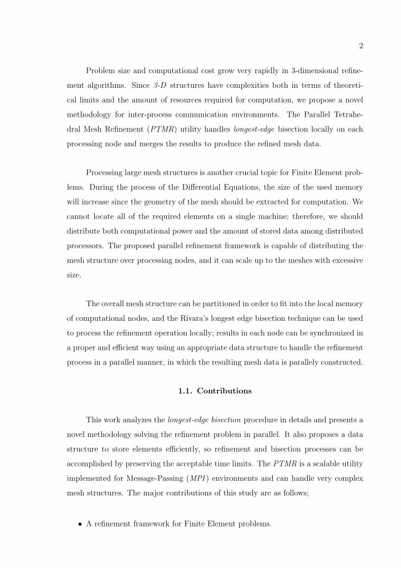
that ordered list will not spread from these origins [2, 4, 20, 24, 25, 27].

Two neighboring triangles that share a common longest-edge will be called a pair.

If a triangle does not belong to any pair of terminal triangles, it will be called a single

triangle [24].

Figure 2.1. Longest-Edge Bisection of Triangle t0

Figure 2.1 shows the LEPP (t0)={t0, t1, t2, t3}, propagation path for triangle t0.

Triangulation of refinement problems can be solved via evaluating the longest-edge

propagation path. We can compute the LEPP and bisect elements in the list to

accomplish the refinement process. If the triangle is a terminal boundary triangle,

we bisect t; otherwise, we bisect the last pair of terminal triangles in the LEPP [3, 5,

6, 7, 17, 23]. In the given example, terminal triangle pairs t3 − t2, t2 − t1, t1 − t0 will be

bisected in order. This procedure, starting from an initial conforming geometry, will

produce a good-quality nested triangulation with linear time complexity [2, 4, 20].

The Longest-edge Propagation Path algorithm, shown in Figure 2.2, can be gener-

alized to 3 -dimensional tetrahedral mesh structures. The 3-D LEPP for a tetrahedron

⊺, is the set of neighboring tetrahedra that have adjacent longest-edge greater or equal

to the preceding tetrahedra in the list [3, 4, 9, 12, 24, 26]. A terminal tetrahedra set is

the set of tetrahedra that share a common longest-edge [4].

7

Longest-Edge Bisection Algorithm (T , t):

1. While there is a triangle t not bisected

2. compute LEPP (t)

3. if t is the boundary terminal triangle

4. bisect(t)

5. else bisect the last pair of terminal triangles in LEPP (t)

Figure 2.2. Longest-Edge Bisection Algorithm from Rivara [4]

2.2. Analysis of the Propagation Path

Numerical experiments have demonstrated asymptotic behavior of the refinement

process and some other characteristics of the generated mesh sequences. While analyz-

ing the refinement process, we can describe it basically as inserting former vertices to

result in well-shaped and conforming triangles. The produced mesh structure should

not lead to unexpected effects in terms of numerical stability and accuracy [2, 7].

Mesh conformity and mesh smoothness can be summarized as [6, 24];

• Intersection of adjacent triangles is either a common vertex or an edge.

• Transition between small and large elements should be gradual.

Longest-edges are bisected progressively so all angles in triangle refinement are

greater or equal to half of the smallest angle in the initial mesh geometry [1, 4, 5, 6,

20, 23]. Thus, known longest-edge refinement algorithms guarantee the construction

of smooth and conforming structures.

Longest-edge bisection can propagate to the entire mesh in worst cases. Propa-

gation is accomplished by traversing the Longest-edge Neighbor Triangles of triangle t.

The neighboring triangle of t is the triangle that shares the longest-edge with t. Figure

2.3 describes an eccentric situation. However, theoretical results and experiments show

that successive processing of unstructured triangular mesh refinement results in mesh

structures in which the average propagation path is reduced in each refinement stage

8

and approaches to the constant of 5 [24].

Figure 2.3. Longest-Edge Propagation

Four Triangle Longest Edge Partition(4T-LE ) divides a triangle t into four sub-

triangles such that the original triangle is bisected by its longest edge and then two

new resulting triangles are bisected by joining the midpoint of the longest-edge with

midpoints of the edges from original triangle t. In a single refinement stage, a triangle

can be bisected into four sub-triangles [2]. According to the processing of the algorithm

and evaluation of LEPP, a triangle can be partitioned into lesser sub-triangles. Figure

2.4 shows the possible 4T-LE if the longest-edge is chosen for bisection.

Figure 2.4. 4T-LE Refinement

Another concept defining the characteristics of the LEPP is the balancing degree.

If triangular geometry contains n triangles and m of them are in pairs of terminal

triangles, then the LEPP -balancing degree of triangulation is defined as n

m. LEPP -

balancing = 1 means that all triangles are in terminal pairs and that there is no

terminal boundary triangle [24]. M1(t) is defined as the sum of the lengths of the

LEPPs’ of the neighbors of triangle t. M2(t) is defined as the maximum length of

9

the LEPPs’ of the neighbors of triangle t. For a triangular mesh structure in which

LEPP -balancing degree ≃ 1, M1(t) ≃ 5 and M2(t) ≃ 2 [24].

For 2 -dimensional mesh refinement, we can restrict the length of the propagation

path. This behavior is crucial in terms of analyzing the algorithms and performance of

the bisection process. However, such a limitation cannot be stated for 3 -dimensional

tetrahedral meshes. It should be noted that this property is the most important dif-

ference between 2 -dimensional and 3 -dimensional refinement algorithms; lack of such

a limiting definition (M1(t) ≃ 5 in 2-D) results in the challenge for 3 -dimensional

problems.

LEPP of a triangle t is always finite and elements in the propagation list have

strictly increasing edge lengths [4]. Terminal-edge points to the end of a propagation list

in which a refinement path will not propagate anymore. They are utilized in refinement

algorithms for 2-D and 3-D structures to define stopping points in a propagation graph.

The edge which is longest in the near area is supposed to be a terminal-edge, so all

terminal edges can be refined safely until the mesh structure conforms specifications.

Refining a terminal-edge will not affect conformity of the mesh [24, 26].

Figure 2.5. Longest-Edge Propagation Path (a) 2-D (b) 3-D

10

In 2-D meshes, a LEPP-graph forms a forest since each edge can only have two

neighbor triangles. Each tree in the forest can be used to find the elements that should

be refined for a conforming mesh structure [28].

A propagation path for 3-D mesh forms a directed-acyclic graph (DAG) such

that each longest edge can be shared by many triangles and refinement operation can

propagate in many directions. Therefore, the Longest-edge propagation graphs for 3-D

meshes are denser. Figure 2.5 is an example of LEPP for 2-D and 3-D structures.

The LEPP graph can be sequentially processed with O(n) time complexity [1, 2,

6, 7, 29, 30]. Parallel implementation can be handled in O(logn) time if the structure

is 2-D [28]. However, it cannot be stated for 3-D mesh, since the number of edges in

the propagation graph is not linearly related to the number of elements as in a LEPP

graph of a 2-D mesh.

On the other hand, numerical experiments demonstrate an asymptotic behavior

of mesh sequences for the 4T-LE refinement. The propagation path extend to a few

neighboring adjacent triangles [24]. This information is used to analyze and prepare

a refinement algorithm for 2-D triangle meshes. The number of elements that should

be refined is related to the elements in the LEPP graph, and this property proves the

practical advantages for longest-edge mechanism.

2.3. Skeleton Algorithms

The 8T-LE partition is defined in terms of a polyhedron skeleton concept using

a simple edge-midpoint bisection procedure. The 2 -dimensional algorithm, which is

also formulated as 4-triangle longest-edge, works over wireframe meshes containing

the edges of target triangles and some neighboring triangles to prepare a conforming

structure [15, 2, 25, 27].

Information in the lower dimension is used to partition appropriate triangles. The

8-tetrahedra algorithm is the generalization of skeleton algorithms in 3 -dimensions.

11

Figure 2.6 represents the 2 -dimensional view of a tetrahedron. Volume refinement is

based on the partitioned triangular faces of the tetrahedron in 2 -dimension [1, 3, 4].

Four-triangle partitions or partial partitions of neighboring triangles are accomplished

by using edge bisection; that is, by refining the wireframe mesh of the 3 -dimensional

edges of tetrahedra [12, 25].

Figure 2.6. 2-D Skeleton

The 4-Triangle algorithm produces a finite number of distinct triangles that are

embedded in the parent. Figure 2.7.a shows the partition patterns of 4-Triangles

longest-edge. The refinement process generates triangles that have the smallest an-

gle greater or equal to α/2 where α is the smallest angle in the original mesh [6].

Continuing refinement iterations produce a stable molecule around a vertex for a local

refinement of a conforming triangulation; angles of the vertex are not divided in the

next operations [6, 7, 22]. Figure 2.7.b shows the fractal property of 4-Triangle method.

The skeleton algorithm for 4-Triangle mesh refinement can be analyzed in two

steps; bisecting the edges in a 1 -dimensional skeleton and partitioning individual tri-

angles according to the bisected edges [9, 25]. The 3 -dimensional skeleton algorithm

is a generalized version of 4-Triangles. If tetrahedral mesh τ is conforming, then 2-

D skeleton, which is the triangular faces of the elements of τ , is also conforming [3].

Moreover, a 1-D skeleton of τ tetrahedral mesh is a conforming wireframe mesh of the

elements of τ [3, 9, 25].

We can basically define the 3D algorithm as;

• Partition edges over 1-D skeleton.

12

Figure 2.7. (a) Refinement Patterns of 4-Triangle. (b) Stable Molecule Behavior of

4-Triangle.

• Partition faces over 2-D skeleton that are involved in the refinement.

(4-Triangle LE )

• Partition involved tetrahedrons according to partition patterns.

(8-Tetrahedra LE )

The 8-Tetrahedra longest edge partition is a 3-D algorithm that can be explained

by applying 4-Triangle skeleton refinement methodology to the faces of corresponding

mesh τ [3]. Partitioning any tetrahedron ⊺ in mesh τ produces both conforming volume

mesh and conforming surface mesh.

2.4. 8-Tetrahedra Longest Edge (8T-LE)

We need some definitions related to 8-Tetrahedra Longest-edge partition. Two

primary faces of any tetrahedron ⊺ are the faces that share the unique longest edge.

The remaining faces are the secondary faces of the tetrahedral [3, 9]. The secondary

longest edges are the longest edges of secondary faces. The remaining edges are called

third-class edges. There may be one secondary longest edge and four third-class edges,

13

Figure 2.8. 4-Tetrahedra and 8-Tetrahedra

or two secondary longest edges and four third-class edges, a total of 6 edges in the

tetrahedron.

We assume there is a unique longest edge that is also the longest edge of two

primary faces and that there are unique secondary edges [1, 3, 15]. In order to prevent

confusion, a unique selection is required during the progress of the refinement algorithm.

The overall structure of the 8T-LE can be defined as follows;

• Longest edge bisection produces two tetrahedron ⊺1and ⊺2.

• Bisection of ⊺1 and ⊺2 according to the longest secondary edges of ⊺ produces

⊺11, ⊺12 and ⊺21, ⊺22 (4-Tetrahedra).

• Bisection of each 4 sub-tetrahedra according to the midpoint of the remaining

edges of ⊺ produces 8 sub-tetrahedra.

If we bisect the tetrahedron with its longest edge, and continue partitioning with

14

secondary edges there will be 4 sub-tetrahedra that do have a unique third-class edge

of the original tetrahedron ⊺. Such a volume triangulation which is called 4-Tetrahedra

will not be conforming only if secondary edges share a vertex and one of those edges is

opposite to the longest edge of ⊺. It is claimed that there are four possible translations

of 4-Tetrahedra partition [3];

• There is only a single secondary edge, and it is opposite to the longest edge of ⊺.

• Secondary longest edges and longest edge of ⊺ are the three edges of a triangle

in the tetrahedron.

• Secondary longest edges are opposite each other, and both share a vertex with

the longest edge of ⊺.

• Secondary edges share a vertex and one of them is opposite to the longest edge

of ⊺.

Only the first three cases produce conforming triangulation. Therefore, 8T-LE

which supplies overall conformity by bisecting each of four sub-tetrahedra by non-

bisected third-class edges of ⊺ is the utilized methodology in 3-D refinement. It is

proven that such a partitioning for all 4 cases produces conforming volume triangulation

for any tetrahedron [3]. Figure 2.8 show the 4-Tetrahedra and 8-Tetrahedra longest-

edge bisection schemes.

Properties of tetrahedral meshes have been studied by many researchers [3, 4, 9,

12, 11, 13, 14, 15, 16, 17, 24]. The 8T-LE partition pattern is the latest methodol-

ogy used in the refinement process [3, 4]. Volume triangulation with 8 new internal

tetrahedra occurred and each face has been partitioned into 4 triangles. There is an

interior edge from the midpoint of the longest-edge of ⊺ to the midpoint of the edge op-

posite the longest-edge. Such a triangulation produces conformity both in volume and

surface structure. Surface structure is identical to the pattern obtained by 4-Triangle

partitioning.

15

3 − D Algorithm-Refinement of a tetrahedron ⊺ in 3 − D mesh τ :

1. For each edge e of tetrahedron ⊺

2. Add e into Eselected

3. While Eselected is not empty

4. Process an edge e from Eselected

5. For each face f sharing edge e

6. Select the longest-edge LE of face f

7. If LE has not been processed before

8. Add into Eselected

9. For each edge e in Eselected (1-dimensional)

10. Bisect edge e

11. For each face f , including any bisected edge e (2-dimensional)

12. Partition face f according to bisected edges

13. For each tetrahedron including any partitioned face f (3-dimensional)

14. Partition tetrahedron according to bisected faces

Figure 2.9. 3-D Refinement Algorithm

2.5. 3-D Sequential Algorithm

The 3-D algorithm for refining any tetrahedron ⊺ in a conforming mesh τ is

a generalized version of a 2-D skeleton refinement algorithm. The volume structure

of the refined mesh based on the 8T-LE also produces the refined 2-D skeleton sur-

face structure. Moreover, refinement of the faces of ⊺ as a 2-D skeleton structure in

tetrahedra mesh τ produces a refined 2-D volume structure.

The sequential algorithm for 3D skeleton refinement is finite with linear complex-

ity O(n) [3]. The longest-edge procedure described in previous sections is used in the

refinement algorithm which is shown in Figure 2.9.

16

3. PARALLEL ALGORITHM

Because of the excessive size of mesh structures used in current research projects,

developing a parallel refinement algorithm is a crucial topic for Partial Differential

Equation (PDE ) problems. There are many related projects investigating an effective

procedure that is applicable to adaptive meshes [29, 31, 32, 33, 30, 34, 35, 36, 37, 38,

39, 40, 41].

The most recent methodology for parallel refinement is based on terminal edges,

which are defined as edges that do not propagate and do not cause other elements to

be refined [26]. The Terminal-Edge Bisection procedure has sequential and parallel

solutions, and the main idea is to bisect the terminal-edge which is the longest among

selected edges first and to continue this process until all of required elements are refined

[26]. However, there are some drawbacks in such a solution like partitioning more

components than required and increasing the number of elements in the resulting 3-D

structure, which already necessitates an extreme number of resources. This solution

may not be practical despite the flexibility of the proposed technique.

There are many other solutions for refining 2-D triangular meshes in a parallel

manner, and those methods are rather different from the parallel techniques used for

tetrahedral mesh structures [28, 30, 32, 33]. Remote references pointing to elements

located in other processors are used for the parallel implementations, and there are

also some approximation methods suggested to handle the refinement problem.

Since the refinement process is one of the underlying computational parts of the

main PDE problem, the solution should be flexible and simple enough to integrate

with other components.

In this chapter, we analyze the longest-edge propagation graph for the parallel

refinement process and present the proposed algorithm for 3 -dimensional mesh re-

finement in a parallel manner. First, properties of the propagation graph, directed

17

acyclic graph, is described. We describe the difficulties for 3 -dimensional algorithms

and compare them with 2 -dimensional approaches. Finally, we present the proposed

3-D algorithm for tetrahedral mesh refinement in distributed environments. The 3-D

algorithm for distributed environments uses the 8T-LE technique to process and find

elements that will be refined.

3.1. The Longest-Edge Propagation Graph

Initially, we may find the propagation paths of faces and associated tetrahedra.

Instead of processing in an recursive manner and deciding whether or not to refine

the element in the sequence, the algorithm will select first the components that should

be refined, and process them independently. The final mesh structure will also be

conformed according to the longest-edge propagation criterion [26, 28]. Therefore,

the data structure used in the implementation should provide both relations of faces

in terms of neighborhood and shared longest-edges for 3-D mesh τ . Preparing the

propagation graph for the refinement, which is a Directed-Acyclic Graph (DAG), is the

first step of the overall algorithm. It can be parallelized since each component such

as edge and face has enough information to form the relationship graph without any

dependency or requirement.

All other nodes that can be reached from v in LEPP -Graph should be processed

in order to accomplish the refinement operation. Since the LEPP -Graph is prepared

according to the length of the edges, and each node represents one of the longest edges

in the initial mesh, when we go through elements in a propagation path, the length of

nodes increases. Therefore, one method is to sort nodes according to the length and

then compute propagation path. The Terminal-Edge Bisection procedure performs the

refinement process in a similar manner; however, it only interacts with the last element

of the propagation path [26]. After the bisection of the terminal-edge, the previous

node in the path will be selected in the next sequence, and the propagation situation

will be completed without necessarily computing all reachable edges [26].

Figure 3.1 shows the reachable nodes from a selected element in order to represent

18

the characteristics of the LEPP -Graph for 3-D structures. On the other hand, storing

and computing all of the reachable elements are inappropriate due to required memory

and computational requirements.

Figure 3.1. LEPP -Graph

3.2. Longest-Edge Refinement

The sequential longest-edge bisection algorithm traverses all edges and select

elements that must be refined, and the overall process is handled by first visiting faces

that have longer longest-edges. Some studies have proposed algorithms which process

bisection after the selection of all components marked to be refined [1, 3, 4, 9, 17, 26].

It has been theoretically proved in recent studies that produced mesh structure is a

conforming mesh in the longest-edge refinement. Figure 3.2 presents the bisection

algorithm; the LEPP is processed while traversing the overall mesh.

In order to parallelize the algorithm, we should select the longest edge of each

face. We assume that each face f has a unique longest edge and also each tetrahedral

19

3-D Skeleton Refinement Algorithm (τ,⊺)

/* Find involved edges, faces, and tetrahedra */

1. Initialize SE, SF , and ST ;

respectively sets of involved edges, faces, and tetrahedra.

2. Initialize PE, set of processing edges

3. for each edge e of ⊺

4. add edge e to set SE

5. add edge e to set PE

6. While PE 6= ∅, do

7. pick e from PE

8. for each tetrahedron ⊺ sharing edge e

9. for each face f of ⊺ having an edge in SE

10. find longest-edge e of f

11. if e is not in SE

12. add e to SE

13. add e to PE

14. add f to SF

15. add t to ST

16. Partition involved edges

17. for each edge e in SE

18. create vertex v midpoint of e

19. bisect e

20. Partition involved faces

21. for each edge F in SF, do

22. partition f according its bisected edges.

23. Partition involved tetrahedra

24. for each tetrahedron ⊺ in ST

25. partition ⊺ according to the partition of its faces.

Figure 3.2. 3-D Skeleton Refinement Algorithm from Plaza and Rivara [3]

20

Figure 3.3. Propagation Path

has a unique longest edge according to 8T-LE ; thus, there must be a unique selection

procedure. Each face is pointed with its longest-edge and we start from the edges of

the tetrahedral that is going to be refined in a conforming mesh. Figure 3.3 and 3.4

presents the idea of longest-edge selection and the concept of traversing the propagation

path in 3-D bisection steps. In this example, selection of edges BC and CD result in

propagation to the longest-edges of other faces in the mesh structure.

3.3. 2-D versus 3-D

Theoretical limits for parallel tetrahedral mesh refinement depend on the process-

ing of the LEPP graph. It states the elements that are affected after an initial tetra-

hedron refinement. If we compute and mark those elements to be refined, other parts

such as bisection steps are easily handled in a parallel environment since they will not

depend on one another.

The propagation graph does not have a specific property that can be used to find

reachable elements within a parallel algorithm. On the other hand, there are some ap-

proaches for similar methodologies; the LEPP graph is a directed-acyclic graph(DAG)

and the DAG can be evaluated in many parallel ways. Most of the related techniques

use random algorithms and state effective complexity times [42, 43, 44, 45, 46, 47, 48].

Average complexity may have proper values, but worst case complexity is not accept-

21

able when compared to sequential algorithms. Those parallel techniques are probably

not practically applicable for mesh refinement; the refinement process is another sub-

component of the PDE problem and should be simple enough for the implementation.

The sequential algorithm has complexity O(n); when data is distributed and

evaluated in a parallel manner, we should deal with the relations between propagation

paths. In 3-D, each element in the LEPP graph can have more than one propagation.

Thus, the number of edges in the LEPP graph, which are keeping the propagation

relationship, is O(n) [13, 26, 49, 46, 47], if n is the number of elements. Therefore,

we can process LEPP graphs in O(logn) time with n2 processors. For the 2-D algo-

rithm, elements propagate to only one other element, and the number of edges in the

LEPP graph is O(n) ; thus, the LEPP graph can be processed in O(logn) time with

n processors.

3.4. Algorithm for Distributed Environments

We start from an initial tetrahedron ⊺, refine according to LE -bisection and

progress to find other elements that must be partitioned. The second step is selecting

all remaining components that should be refined to form a conforming mesh structure.

Propagating through the initial components will lead us to all other elements that

corrupt the conformity.

The next step is combining components to form a conforming mesh structure.

Due to the nature of structural algorithms, explained in the previous chapter, we refine

faces according to the refined one-dimensional edges; and refine tetrahedron according

to 2-D faces. Components in former steps represent the edges in the one-dimensional

skeleton.

The parallel algorithm can be analyzed in three steps:

• Prepare propagation graph for the refinement, (DAG) for 3-D mesh τ .

• Find components which must be refined.

22

• Partition components according to the longest-edge bisection procedure.

The 3 -dimensional mesh refinement solution for adaptive structures should be

effective in terms of scalability, distributed costs, and partitioned data. Required

memory for tetrahedral mesh structures increases if compared to 2 -dimensional struc-

tures. Therefore, distributing the computational power with partitioned data structure

is crucial if large structures are concerned.

The distributed algorithm accomplishes refinement problems by utilizing the local

bisection procedure and synchronizing partitioned tetrahedra. Since propagation-paths

are distributed, terminal points for a local mesh may trigger to another LEPP globally.

In Figure 3.5, we demonstrated the overall algorithm.

The propagation path is distributed among each processor, and they compute lo-

cal LEPP -Graphs independently. After the local refinement process, computing nodes

are informed to trigger the refinement if the border element of the local mesh partition

is selected to be bisected by another processor. Figure 3.6 presents the logically parti-

tioned LEPP -Graph. In the given example, overall structure is partitioned among 3

processors. Node 13 and 14 have a common longest-edge; thus, refining Node 13 rep-

resenting a tetrahedron in the figure results in propagation of the LEPP and refinement

of Node 14. The other processor is informed that neighbor node in the border of the lo-

cal partition should be refined. Therefore, the LEPP graph of the local mesh structure

is synchronized and the integrity of the overall propagation paths is preserved.

The synchronization process is limited and cannot exceed a few loops due to

the conforming structure of input mesh structure. The previous chapter analyzes the

LEPP features and states that the depth of the propagation graph does not increase

dramatically, especially for 2-D structures. In real-life problems, we usually start to

refine some tetrahedra, causing an unacceptable error ratio in a PDE problem. Such

a situation will not propagate to all other elements of the mesh; thus, handling large

mesh structures and distributing them among remote processor to compute at the same

time is more important. Figure 3.7 presents the flow-chart representation.

23

Figure 3.4. Longest-Edge Selection

24

Distributed Algorithm(P processors, Tetrahedral Mesh τ ):

1. Distribute the Tetrahedral Mesh Structure τ among processors,

2. Each processor Pi handles its local mesh structure.

3. Process the Longest-Edge Algorithm locally:

4. foreach edge e of tetrahedron ⊺ that needs to be refined

5. add edge e to the list of selected edges Eselected

6. LEPP algorithm:

7. while all edges in Eselected are processed

8. if LE of the face f that edge e belongs is not selected

9. add edge LE to the list of selected edges Eselected

10. add tetrahedron ⊺ that edge e belongs to

the list of selected tetrahedra Tselected

11. Synchronize local Propagation Paths:

12. if local terminal point in the LEPP also belongs to another

local mesh structure τ owned by processor Pi

13. inform processor Pi

14. Process the LEPP algorithm after synchronization.

15. Bisect selected edges Eselected

16. Bisect selected tetrahedra Tselected

17. Collect local mesh structure from processing nodes, Pis

Figure 3.5. Distributed Algorithm

25

Figure 3.6. LEPP -Graph Partitioning and Synchronization

26

Figure 3.7. The PTMR Algorithm

27

4. IMPLEMENTATION DETAILS

Parallel Mesh Refinement algorithms have been studied for 2-D and 3-D struc-

tures. In 2-D triangular mesh, we can utilize the longest-edge refinement technique to

prepare a parallel implementation. Since propagation to neighbors of an element can-

not be limited as we can state in 2-D, tetrahedron mesh refinement has difficulties in

terms of parallelization. Most of the proposed parallel models use some approximation

techniques to prepare a conforming mesh instead of concluding with the most proper

mesh structure. Features of the tetrahedron mesh such as average and maximum in-

teraction of elements in a proper conforming structure have been studied, but those

properties are not sufficient to be used for the refinement implementation in parallel.

We have studied theoretical properties of refinement to investigate a proper par-

allel algorithm with logarithmic complexity for tetrahedron mesh structures. Some

models to handle the parallel refinement have been proposed; however, they are not

practically applicable due to scalability reasons. Processing of the propagation-path

with the computation of all reachable elements results in very poor performance com-

pared to those algorithms for the sequential refinement. Therefore, we decided to study

practical implementation of the problem in distributed environments.

Parallel Tetrahedral Mesh Refinement (PTMR) implementation can be encapsu-

lated and used by other Finite Element programs; thus, it provides a framework for

the refinement process. Initially, distribution of the elements among processing nodes

is accomplished. The mesh object is loaded locally and prepared for the refinement

operation. After finishing the refinement process, master processor collects new ver-

tices and tetrahedra. Another important feature is the profiler; that is, all methods

are also capable of collecting elapsed time information in the network communication

and computational code segments.

The parallel framework for tetrahedral mesh refinement, PTMR, requires MPI

[50] and PaRMetis [51] libraries. Loaded mesh is partitioned in order to have mini-

28

mum edge-cuts in the LEPP -Graph. Mesh partitioning is accomplished according to

tetrahedra, and each processor keeps only the elements that are assigned. The mesh

structure is partitioned fairly concerning the network cost between processing nodes.

The overall mesh geometry fits into the memories of each processing nodes; thus, we

can handle tetrahedral mesh files with excessive memory requirements. The most im-

portant advantage of PTMR is the scalability; we can not deploy a very large mesh

structure on a single node due to memory limitations, but we can distribute the data

and operate in a parallel manner.

Tetrahedrons that should be refined initially are computed, and other elements

which will be affected are selected using the LEPP. The selection procedure is accom-

plished by traversing the mesh data in the local processing node. A refined edge in one

of the processors can trigger another tetrahedron which is in another processor’s local

memory. Therefore, related processing nodes are informed if an edge will be refined in

the border of a partition.

Procedure of the parallel implementation can be stated as follows:

• Partition and distribute tetrahedral mesh elements.

• Compute initial tetrahedrons that should be refined.

• Prepare the local LEPP -Graph sequentially and select the edges that should be

refined.

• Inform other processing nodes whether a border element in the local partition is

selected.

• Refine according to the 8T-LE procedure.

• Collect mesh data with recently produced tetrahedrons.

The gateway node is used not only to read the initial mesh data from file but also

to prepare communication objects holding the information whether border elements

of the local mesh partition require refinement or not. Therefore, the gateway node

minimizes the number of network messages, and this situation is an important issue

to enhance the performance of an MPI program [50, 52]. Each processing node sends

29

the information about the selected border elements to be refined with the knowledge

of neighbor processors that should take action. The gateway node collects the effected

elements and informs other processors to start refinement process for the classified

element.

4.1. Data Structure

Designing a proper data structure is another challenge in the implementation.

Some know techniques have been investigated [53, 54, 55, 56, 27, 57] in order to pre-

pare a flexible architecture for the PTMR. A mesh structure is formed of vertices,

edges, triangles and tetrahedrons. In order to process algorithms, we should be able

to evaluate each element and keep relations between them. The 8T-LE algorithm is a

skeleton algorithm, and elements in lower dimensions are required for refinement. It is

stated that the number of tetrahedrons in a conforming mesh is much more than the

number of other elements; and any tetrahedron is adjacent to many edges and vertices

[58]. Figure 4.1 demonstrates the number of elements of a conforming mesh on average.

Relations between elements are the related adjacencies; as an example, changing an

edge will affect 5 tetrahedra on average [58].

Since the 8T-LE is not principally parallelizable due to the sequential progress

of Longest-Edge propagation, we developed a new data structure with a convenient

parallel algorithm which is applicable to distributed environments. During the imple-

mentation of distributed algorithms in PTMR utility, we keep adjacency relationships

between edges and tetrahedrons. Each tetrahedron object keeps the list of edges it

owns, and edge objects have the list of vertices that form itself. Edge objects also

have the list of tetrahedrons which are adjacent, so that, while evaluating the LEPP,

computation can be handled without searching adjacencies each time.

The data structure of the local mesh object has vertices, edges and tetrahedra.

Each edge object has the list of tetrahedra it is owned by. The tetrahedron object

keeps the list of edges that form this tetrahedron, and we can calculate the information

of faces when required in the propagation path process.

30

Each vertex object has a single unique identifier which distinguishing them in the

global space. Each processor starts from a sequence which will not intersect with other

processors. During the operation of the LEPP synchronization, a unique identifier

which is the smallest number among all other local sequences, is selected as the identifier

for the effected neighbor elements in the border of a local structure.

In 8T − LE and 4T − LE, we must select the longest-edge and that should be

unique in the tetrahedron or in the triangle. The edge object has a simple methodology

to handle the uniqueness for the length comparison. If the length of two edges are equal,

identifiers of the first and then the second vertices are compared to select one of them

as the longer edge.

Figure 4.2 shows the used data structure skeleton. Figure 4.5 presents a more

detailed view of the data model which is also evaluated in Appendix A.

Figure 4.1. Statistics for the Number of Entities of a Mesh from Garimella [58]

Mesh structure is partitioned between each processing node according to cost of

interaction between elements. Thus, while synchronizing the LEPPs between compo-

nents, the parallel tetrahedron refinement process minimizes the network and compu-

tational costs. Such an implementation also covers the scalability objective. Moreover,

the gateway node used in the algorithm enables us to minimize the number of network

messages. PTMR uses communication objects in the MPI environment in order to

31

Tetra

Face

Edge

Vertex

Figure 4.2. Data Structure of PTMR

Figure 4.3. Mesh Refinement Example

minimize the network traffic and handle the dynamic data transfer between proces-

sors. Each processing node uses the synchronization information to select and start

the refinement from received elements if it is required. Synchronizing the borders

of propagation graph, which is partitioned among processors as a result of the local

mesh processing, is accomplished by summarizing the received bisection information

and distributing among the concerned processors. Since the gateway node collects all

messages used to synchronize the overall LEPP, it prevents duplicate messages in the

communication environment.

Parallel implementation for distributed environment has been prepared and tested

32

Figure 4.4. Mesh Refinement Example

for homogenous platforms. Utilized data-structure can also handle heterogeneous en-

vironments and is capable of adapting to data distribution. Test results about the

proposed methodology of refinement process are presented in the next chapter. Since

data is properly distributed, we can separate and reduce the overall computation and

memory cost of the refinement process. Figure 4.3 and 4.4 show produced tetrahedral

mesh results.

33

Ref erence top arents if created by bisecting an edge

Ref erence to sub�edges af ter bisectionRef erence to the mid�p ointp roducedaf ter selecting thisList of tetrahedral that own this edge

Ref erence to Tetra�bucket that tetrahedron resides

List of tetrahedra that are in this bucket obj ectNeighbourp rocessor that also own tetrahedralof this obj ect

Ref erence top arents if created by bisecting an edge

Ref erence to sub�edges af ter bisectionRef erence to the mid�p ointp roducedaf ter selecting thisList of tetrahedral that own this edge

Ref erence to Tetra�bucket that tetrahedron resides

List of tetrahedra that are in this bucket obj ectNeighbourp rocessor that also own tetrahedralof this obj ect

Figure 4.5. The Object Relationship of the PTMR Utility

34

5. TEST RESULTS

Mesh input files from the GAMMA project [59] were used as examples for testing

the PTMR utility. The aim of the GAMMA project is to analyze and develop mesh

generation algorithms which are suitable for Finite Element Computations. Some re-

search topics of the project are Mesh Generation Algorithms, Error Estimation, Parallel

Computing, and Data-structures [59].

We also used mesh generation tools to understand the accuracy of the method-

ology. Some of the mesh inputs were generated by TetGen [60], which is a program

for generating tetrahedral meshes for arbitrary 3-D domains. Mesh generation of the

TetGen program is based on Delaunay methods, and the tool was written in ANSI

C++ [60, 61].

The cluster system with 128 nodes from High Performance Computing Center of

ULAKBIM [62] was used to run test scenarios. Sun Grid Engine (SGE ) [63, 64] is

the Job Management System of the cluster. It is a multi-user environment and two

execution queues were defined for each node; thus, the job scheduler might assign a

node for the execution in which any other process was also running. Moreover, two

processes of a single test job can be executed in one processor; without any network

communication cost between them. Since processes of the PTMR were competing for

computing cycles with another processes in the system, we did sometimes encounter

unexpected results. Configuration of the system in which test scenarios were executed

was not proper to evaluate the performance of the PTMR. Therefore, results for elapsed

time values in test routines did not reflect the actual performance. However, they did

provide an estimation and show that mesh refinement can be processed in a few minutes

by using the PTMR utility.

The following figures present some of the generated mesh files which were pro-

duced by refining sample input structures. Mesh structures were viewed by Medit [65]

35

Figure 5.1. 14904 tetrahedra / 4502 vertices

and Tetview [66] which are graphic programs for viewing tetrahedral meshes.

Refining the tetrahedra mesh in Figure 5.2, which has 1803 tetrahedra and 527

vertices, will produce a new structure with 13506 tetrahedra and 3387 vertices. After

refining the resulting tetrahedral mesh we produced the 3-D formation shown in Figure

5.5 that has 99121 tetrahedra and 23351 vertices. Refinement of mesh in Figure 5.1,

14904 tetrahedra, and 4502 vertices produced 70203 tetrahedra and 22568 vertices, as

shown in Figure 5.6. Refinement of the resulting mesh second time resulted in 235941

tetrahedra and 22568 vertices.

Refinement of the mesh with 12586 tetrahedra and 3644 vertices in Figure 5.4

produced the 3-D geometry of 79263 tetrahedra and 33098 vertices as shown in Figure

5.7. Other test results generated from the same source produced mesh structures with

450573 tetrahedra and138842 vertices, and 770882 tetrahedra and 215017 vertices.

Information about elapsed time for the steps of the program can be viewed via

defining the debugging parameter of the PTMR utility. Figures from 5.8 to 5.10 show

the graphic of performance counts. Figure 5.8 shows the time spent in the gateway

36


node while synchronizing the LEPP graph. According to the Figure 5.8, elapsed time

does not increase as the number of processor increases; thus, the gateway node is

not the bottleneck of the overall algorithm. Mesh structures with 1803, 12586, and

74178 tetras are used for the test case, and the resulting meshes have 74178, 13281,

and 450573 tetras in the given order. Figure 5.9 presents the maximum amount of

time spent in a single processor among processing nodes during the refinement process.

As the number of processors increases, maximum time spent decreases, since data is

distributed among processing nodes.

In Figure 5.10, overall time of the PTMR utility is shown. As can be seen from the

figure, the increase in the number of elements can be handled by using more processing

nodes.

37



38



39


40

00.10.20.30.40.50.60.70.80.91

0 5 10 15 20 25 30 35 40 45 50Number of processors

Ti me( secs) 74178 tetras12586 tetras1803 tetras

Figure 5.8. The Refinement Process According to the LEPP Algorithm (elapsed time

spent in the gateway node)

00.511.522.533.544.5

0 5 10 15 20 25 30 35Number of processors

Ti me( secs)74178 tetras12586 tetras1803 tetras

Figure 5.9. The Refinement Process According to the LEPP Algorithm

41

01234567

0 5 10 15 20 25 30 35 40 45 50Number of processors

Ti me( secs) 13281 tetras / 2844 vert ices74178 tetras / 19877 vert ices450573 tetras / 115321vert ices

Figure 5.10. Overall Time

42

6. CONCLUSIONS

A parallel mesh refinement algorithm for distributed environments is proposed, in

which each processing node works over its local elements sequentially and synchronizes

changes to update the overall mesh structure.

We analyzed the longest-edge bisection algorithm and presented details about

the parallel refinement process. 3-D structures have difficulties especially in processing

the propagation path of selected tetrahedra. We presented a practical and scalable

methodology which is capable of solving refinement problem within acceptable time

limits. Representation of the mesh is also crucial; the data structure must be compact

not to consume so much memory, but it should be flexible and simple for computation.

We explained the proposed objects to accomplish the construction of mesh topology.

We also present a parallel utility, PTMR, that can distribute the mesh data

and process in an inter-process communication environment; thus, clusters of ordinary

nodes can be used to process very large mesh structures.

43

APPENDIX A: PTMR: Reference

Parallel Tetrahedral Mesh Refinement(PTMR) implementation, build for Distrib-

uted Environments, consists of modules that can be encapsulated and used by other

Finite-Element programs; thus, it provides a framework for the refinement process.

PTMR has the following source files and each of them contains independent modules.

• local.h, utils.h, utils.c, table.c table.h, list.h, fmesh.h

• tmesh.h, tmesh.c, map.h, map.c, rank.h, rank.c

• lPoint.h, lPoint.c, lEdge.h, lEdge.c, lTetra.h, lTetra.c, T bucket.h, T bucket.c

• lMesh.h, lMesh.c

• comm.h, comm.c, lp.h, lp.c

• ptmr.c

There are also some facilities used to handle some implementation issues and they

enabled us to prepare useful programming for other code segments of the mesh parti-

tioning. The overall framework is classified as mesh partitioning, local mesh processing

and refinement according to the longest-edge algorithm. We describe each component

in details and specify their important methods and functions.

Initially, distribution of the elements among processing nodes is accomplished.

The mesh object is loaded locally and prepared for the refinement operation. After

finishing the refinement process, master processor collects new vertices and tetrahedra.

MPI_Init(&argc, &argv);

..............................................

rank=rank_form();

process_args(argc, argv,rank_globalRank(rank));

map_new(map, rank, "create map_ object");

tmesh_new(tmesh, "create tmesh_ object ");

tmesh_dist(rank,map,tmesh); // initial distribution

44

lmesh=lMesh_new_load(rank,map,tmesh);

tmesh_destroy(tmesh,"destroy tmesh_ object");

if(rank_processingNode(rank)){

// Processing Node

lMesh_process(lmesh, rank);

lMesh_send_points(lmesh,rank);

lMesh_send_tetras(lmesh,rank);

}else{

// Gateway Node

lMesh_gateway(lmesh,rank);

lMesh_recv_points(lmesh,rank);

lMesh_recv_tetras(lmesh,rank);

fmesh=lMesh_2fmesh(lmesh);

write_fmesh(fmesh,get_args_file_name());

}

lMesh_free(lmesh);

fmesh_destroy(fmesh, "destroy fmesh_ object");

map_destroy(map, "destroy map_ object");

rank_destroy(rank,"destroy rank_ object");

MPI_Finalize();

The following sections explain the implementation issues, clarify some important

functions and present structure of modules used in this work. All methods presented

are also capable of collecting elapsed time information in the network communication

and computational code segments. Output of steps and results of concerned functions

can be viewed whether appropriate debug and timing definitions are set.

A.1. Utilities

Those procedures consist of general definitions and input/output file formats of

the tetrahedral mesh structure.

45

A.1.1. Global Definitions

local.h includes global definitions for all modules. It defines header files that are

required by used libraries; sets and organizes definitions of timing and debug

levels.

/* LOCAL.H */

#ifndef __PTMR__LOCAL_H__

#define __PTMR__LOCAL_H__

/* headers */

#include <stdio.h>

#include <string.h>

#include <stdlib.h>

#include <errno.h>

#include <math.h>

#include <glib.h>

#include <mpi.h>

#include <parmetis.h>

........................................

#ifdef _TIMING_LEVEL_3

#ifndef _TIMING_LEVEL_2

#define _TIMING_LEVEL_2

#endif



#endif

#endif




#endif

46

#endif

A.1.2. Common Utilities

utils.h consists of global definitions and utility functions. It includes some encapsu-

lated macro definitions for memory allocation and other common procedures.

A.1.3. The Dynamic Pointer Array

list.h defines the List object used to hold pointers of the selected edges and tetrahedra

elements in the refinement process.

•List new( List pointer, definition text)

•List getsize( List pointer)

•List setsize( List pointer, size(int))

•List get( List pointer, index(int))

•List add( List pointer, data pointer)

•List del( List pointer, data pointer)

•List print param( List pointer, print function, parameter)

•List free( List pointer, definition text)

A.1.4. The Pointer Table

Table.[ch] defines the data-structure which is using Binary-Balanced Tree. The Table

object is used to keep the relationship between points(vertices) and edges.

•Table get( Table pointer, index 1(int), index 2(int), data pointer(RETURN)):

Returns the corresponding element if exits, else returns NULL.

•Table set( Table pointer, index 1(int), index 2(int) , data pointer):

Sets indices for the corresponding element.

47

A.1.5. Input/Output File Formats

fmesh.[ch] defines the initial mesh structure that is read from an input file. Output

of the overall process, which is the new tetrahedral mesh, is also an fmesh object.

The fmesh object is used to read and write data from or into a file.

/* initial mesh structure that is read from the file */

typedef struct fmesh_ {

int n_point; // the number of points in the mesh read.

int n_tetra; // the number of tetras in the mesh read.

float * points; // coordinates of the points.

int * tetras; // point id’s of the tetras.

}fmesh_;

Methods of the fmesh print debug information such as the number of elements

read and the total time elapsed in the file operations. It searches for filename.ele that

vertex ids’ of each tetrahedron is written and filename.node that coordinates of vertices

is written.

write fmesh and read fmesh are the main functions of this object; the local mesh

structure(the lMesh object) has conversion methods to map the data of the geometry

in order to optimize the processing of this input structure.

The file format suitable for an fmesh object is:

.ele files:

First line:

<# of tetrahedra> <nodes per tetrahedron (4)>

Remaining lines list # of tetrahedra:

<tetrahedron #> <node> <node> ... <node>

48

.ele file example:

4 4 0

1 7 2 3 5

2 7 2 6 1

3 4 2 6 5

4 7 6 2 5

.node files :

First line:

<# of points> <dimension (3)> <# of attributes>

Remaining lines list # of points:

<point #> <x> <y> <z> [attributes] [boundary marker]

.node files example:

7 3 0 1

1 100 200 100 1

2 100 100 100 1

3 200 100 100 1

4 100 100 200 1

5 150 100 150 1

6 100 150 150 1

7 150 150 100 1

•write fmesh(fmesh pointer, filename):

Read the fmesh object from a file.

49

•read fmesh( fmesh pointer, filename):

Write the fmesh object into a file.

A.2. Mesh Distribution

The mesh structure is partitioned fairly concerning the network cost between

processing nodes. The following modules and data structures are responsible for the

distribution of the mesh data; the network cost should be minimized and computational

cost should be balanced. The overall mesh geometry is partitioned and it fits into the

memories of each processing nodes; thus, we can handle tetrahedral mesh files with

huge memory requirements.

A.2.1. Processor Ranks

rank.[ch] defines the rank of a processing node in the overall Processor Cell.

/* rank object */

typedef struct rank_ {

int global_rank; // the rank in the MPI_COMM_WORLD.

int process_rank; // the rank in the processing node.

int global_size; // the number of processors in the

............................// MPI_COMM_WORLD.

int process_size; // the number of processing nodes.

int gateway; // the global rank of the GATEWAY node.

MPI_Comm pcomm; // the communication object.

} rank_ ;

The Gateway node is specialized to read input from the input file and prepare

the initial synchronization of the data mapping and distribution. Therefore, we require

a different communication object originated from the MPI COMM WORLD [50]. The

rank object returns the ranking of the node and classifies processors as processing

50

nodes and gateway node.

A.2.2. Processor Mapping

map.[ch] handles the distribution and the mapping of elements to processors.

/* MAPPING */

typedef struct map_{

int n_element; // number of tetras in the overall mesh.

int * pdist; // distribution array, among processors.

int * edist; // used for redistribution and keeps new id’s.

int * parts; // map elements to processors.

// only gateway node keeps all elements

// for computing the initial mapping.

} map_ ;

The sync map function forms the initial distribution of processors and keeps the

partitioning information. It operates according to the order of execution switch and

works coordinately with the ParMetis [51] methods.

/* sync_map todo switch

_SYNC_MAP_PDIST_INITIAL // form the initial distribution.

_SYNC_MAP_PDIST_SEND // send the pdist object.

_SYNC_MAP_PARTS_CREATE // allocate memory for map->parts.

_SYNC_MAP_PARTS_GATHER // gather map->parts objects.

_SYNC_MAP_EDIST_CREATE // allocate memory for map->edist.

_SYNC_MAP_PARTS_PROCESS // RE-calculate pdist and edist.

_SYNC_MAP_EDIST_SEND // send the edist object.

_SYNC_MAP_PARTS_DESTROY // destroy the parts object.

*/

51

map→parts, tmesh→adj, and tmesh→adjx are originated from the known CSR

format [51]. An example for the Distributed CSR format is shown in Figure A.1.

Figure A.1. The Distributed CSR Format

•sync map(rank pointer, map pointer, todo switch - integer):

process according to the ”SYNC MAP todo switch”.

A.2.3. Mesh Partitioning

tmesh.[ch] defines the mesh object that holds the local elements and distributes the

elements among processors.

/* TMESH */

typedef struct tmesh_ {

int g_point; // the number of points in the overall mesh.

52

int g_tetra; // the number of tetras in the overall mesh.

int n_tetra; // the number of local tetras.

int * tetras; // tetras in the local processor.

float * points; // all points.

int * adj; // adj and adjx keep adjacency

int * adjx; // information between elements.

} tmesh_ ;

The send tmesh function has three operation flags. Initially, a tetrahedra struc-

ture is partitioned without any restriction and send to the processing nodes to compute

the ideal partitioning information.

The partitioning function ipar, uses ParMETIS V3 PartMeshKway from ParMetis

library [51] to compute the new mapping. The data of the tetrahedral mesh is dis-

patched according to the final mapping. Moreover, the ParMETIS V3 Mesh2Dual

procedure is used to prepare the adjacency relationship between neighbor elements

in different processing nodes. The ipar adj function prepares the DUAL graph [51],

and the required information is preserved locally in each node that we build for other

components.

* SEND_TMESH - The todo switch

_SEND_TMESH_INIT //initialize the tmesh_ object.

_SEND_TMESH_TETRAS //send initial tetras.

// to prepare the partitioning.

_SEND_TMESH_SEND //distribute the MESH data.

*/

The ParMETIS V3 PartMeshKway routine is used to compute a k -way parti-

tioning of a mesh on p processors. The mesh can contain elements of different types.

Parameters of the ParMETIS V3 PartMeshKway ;

53

• elmdist array describing how the elements of the mesh are distributed

among the processors.

• eptr, eind arrays specifing the elements that are stored locally at each

processor.

• elmwgt array storing the weights of the elements.

• wgtflag used to indicate if the graph is weighted.

• numflag used to indicate the numbering scheme.

• ncon used to specify the number of weights that each vertex has.

• ncommonnodes degree of connectivity among the vertices in the dual graph.

• tpwgts used to specify the fraction of vertex weight that should be

distributed to each sub-domain for each balance constraint.

• ubvec array of size ncon that is used to specify the imbalance tolerance

for each vertex weight.

• options array of integers that is used to pass parameters to the routine.

• edgecut the number of edges that are cut by the partitioning.

• part partition vector of the locally-stored vertices.

• comm MPI communicator.

The ParMETIS V3 Mesh2Dual routine is used to construct a distributed graph

given a distributed mesh. Parameters of the ParMETIS V3 Mesh2Dual ;

• elmdist array describing how the elements of the mesh are distributed

among the processors.

• eptr, eind arrays specifying the elements that are stored locally at each

processor.

• numflag used to indicate the numbering scheme.

• ncommonnodes degree of connectivity among the vertices in the dual graph.

• xadj, adjncy adjacency information disccussed in previous sections.

• comm MPI communicator.

The tmesh dist function is the base procedure for the initial distribution of the

mesh structure. It prepares the mapping of objects to processing nodes and distributes

54

elements according to this information. The ParMetis also supports heterogeneous

distribution of the elements. Therefore, we can assign different weight degrees to

different nodes and partition data according to the capacity of each node.

/* TMESH_DIST */

sync_map(rank,map,_SYNC_MAP_PDIST_INITIAL+_SYNC_MAP_PDIST_SEND+\

_SYNC_MAP_PARTS_CREATE);

send_tmesh(rank,map,fmesh,tmesh,_SEND_TMESH_INIT+_SEND_TMESH_TETRAS);

//fmesh_ is NULL for processing nodes.

if( rank_processingNode(rank))

ipar(rank,map,tmesh); //parmetis

sync_map(rank,map,_SYNC_MAP_PARTS_GATHER+_SYNC_MAP_PARTS_PROCESS);

sync_map(rank,map,_SYNC_MAP_PDIST_SEND);

send_tmesh(rank,map,fmesh,tmesh,_SEND_TMESH_SEND);

sync_map(rank,map,_SYNC_MAP_PARTS_DESTROY);

if(rank_processingNode(rank))

ipar_adj(rank,map,tmesh);

The tmesh object supports the redistribution of elements among processors. Ini-

tially, elements of the mesh data are distributed fairly according to the load metrics.

After a refinement step, processing nodes that produced many new tetrahedra, will

handle more elements than others. Therefore, the distribution and the mapping can

be recomputed observing the network cost metric; and then, mesh components can be

resynchronized according to new the distribution to preserve the balanced partition-

ing. The T bucket object has suitable methods to export mesh components and import

elements located in other processing nodes during such a redistribution operation.

55

•send tmesh(rank pointer, map pointer, fmesh pointer, tmesh pointer,

todo switch):

Sends and initializes the tmesh according to the todo switch.

•ipar(rank pointer, map pointer, tmesh pointer):

Runs in processing nodes only, prepares the map→parts.

•ipar adj(rank pointer, map pointer, tmesh pointer):

Prepares the DUAL graph from the mesh, fills tmesh →adj and tmesh →adjx.

•tmesh dist(rank pointer, map pointer, tmesh pointer):

Reads the data and distributes among processors.

A.3. Mesh Operations

The data structure of the local mesh object has vertices, edges and tetrahedra.

Each edge object has the list of tetrahedra it is owned by. The tetrahedron object

keeps only the list of edges that form this tetrahedron, and it does not cover the face

information. We can calculate the information of faces quickly when required in the

propagation path process.

A.3.1. The Point Object

lPoint.[ch] defines the vertex object of a 3-D tetrahedral mesh structure. The lPoint

object keeps the coordinates and the identification number of points stored locally

in each processor.

typedef struct lPoint_ lPoint_;

struct lPoint_ {

int id; // id of the Point.

float x,y,z; // x y z coordinates.

float value; // local value for the Point.

56

int referrer_count; // edges referring this object.

lPoint_ * parent1;

lPoint_ * parent2;

} ;

lPoint objects are referred by the edge elements; they have the coordinates and

the value of the vertex at that point for the given differential equation. Since, more

than one edge can refer to a single vertex, the lPoint object is removed when there is

no referrer pointing to the vertex. It also keeps the parents if created in a refinement

processing. Each lPoint object has a single unique identifier which distinguishes them

in the global space. Each processor starts from a sequence which will not intersect

with other processors. During the operation of the LEPP synchronization, a unique

identifier which is the smallest number among all other local sequences, is selected as

the identifier for the effected neighbor elements in the border of a local structure.

Local vertex information is initially loaded from a tmesh object, and processing

nodes uses this information while defining new edges and midpoints. Only the gate-

way node keeps a list of pointers referring to points of the overall mesh. There are

also methods to export the data into the communication object and import from a

communication objects. Only the element in the border of a local mesh partition is

synchronized if it is processed in the LEPP algorithm. Each processor works over its

own elements without concerning the overall mesh structure. When refinement process

is finished, the gateway node collects all new points from processing nodes and operates

on them to prepare the final list of vertices of the total mesh structure.

•lPoint load initial(rank, number of points,points a[0]=x,a[1]=y,a[2]=z, ..):

Loads the initial lPoint object from the array of coordinates.

• lPoint point2comm(comm pointer, lPoint LIST):

Exports all data to communication object to transmit to the gateway node.

57

• lPoint comm2point(comm pointer, table pointer, lPoint LIST):

Gets points from a comm object and process them.

A.3.2. The Edge Object

lEdge.[ch] defines the object that holds edge information in the local mesh structure.

typedef struct lEdge_ lEdge_;

struct lEdge_ {

lPoint_ *point1; // Point A.

lPoint_ *point2; // Point B.

lPoint_ *midpoint; // midpoint between A and B.

lEdge_ *subedge1; // sub-edges.

lEdge_ *subedge2;

List_ *tetras; // tetras that are neighbors of this edge.

int status; // STATUS of the EDGE object.

float length; // length of the EDGE.

};

The lEdge object keeps the tetrahedra which are adjacent and own this edge.

Each edge object has a list of pointers to the neighbor tetrahedra. According to the

LEPP algorithm, edges are selected and partitioned concerning the skeleton concept.

During the refinement process and other mesh operations, we need to obtain the

correct edge between two points. Thus, the table of pointers is used to find and reserve

the address of a lEdge object. In 8T-LE and 4T-LE, we must select the longest-edge

and that should be unique in the tetrahedron or in the triangle. The edge object has a

simple methodology to handle the uniqueness for the length comparison If the length

of two edges are equal, identifiers of the first and then the second vertices are compared

to select one of them as the longer edge.

58

• lEdge select ( lEdge pointer, LIST newpoints):

Changes the status if selected, and creates the midpoint;

assigns an unique id for the midpoint.

• lEdge divide( lEdge pointer):

Divides the Edge, two new sub-edges are created.

• lEdge get( table pointer, lPoint pointer point 1, lPoint pointer point 2 ):

Finds and returns the edge between point 1 and point 2, creates the edge if not found.

• lEdge list divide all( lEdge LIST, starting index):

Divides all edges in the list starting from a given index.

A.3.3. The Tetrahedron Object

lTetra.[ch] defines the object that holds tetrahedra elements of the mesh structure.

typedef struct lTetra_ {

T_bucket_ * tbucket; // pointer to the T_bucket_ object.

lEdge_ * edges[6]; // edges of the tetrahedron.

int status; // status of the tetrahedron.

// (_TETRA_NEW, _TETRA_SELECTED, _TETRA_DIVIDED)

}lTetra_ ;

Tetrahedra are stored in a tetra bucket (The T bucket object), and each tetra-

hedron has a pointer referring to its owner bucket. In order to simulate the Finite

Element problem situation, we calculate the volume of each element and select the

tetrahedron which has a larger volume than the specified. Selected elements will be

marked to be refined and this information will be passes to the longest-edge refinement

process as the initial input.

59

During the executing the LEPP -algorithm, we should propagate to the other

elements that must be refined in order to conform the proper mesh structure. We

should cover the 2-D structure and check longest-edges of neighbor faces. Initially,

selected edges are the edges of the selected tetrahedra; after the propagation process,

new tetrahedra will be selected to be refined, and their addresses will be stored to be

partitioned.

inline void lTetra_lepp_face( lTetra_ * lTetra_ptr, lEdge_ * edge,

List_ * edge2refine,List_* newpoints){

........................................

lTetra_2points_except(lTetra_ptr, &pointA, &pointB,

(edge)->point1, (edge)->point2);

lTetra_edge_FIND(lTetra_ptr, pointA, (edge)->point1, edgeA);

lTetra_edge_FIND(lTetra_ptr, pointA, (edge)->point2, edgeB);

if(!lEdge_if_selected(edgeA) && !lEdge_if_selected(edgeB)){

le= lEdge_compare_res(edge, edgeA);

le= lEdge_compare_res(le, edgeB);

if(le != (edge)){

lEdge_list_ADD(edge2refine, le,newpoints);

........................................

The information of faces is computed according to the longest-edge algorithm for

2-D structures. The new edge marked to be refined has also the information of effected

tetrahedra that own this element.

While partitioning a tetrahedron according to the 8T-LE, we divide each element

into two subcomponents; and then, we continue partitioning process in those new sub-

elements.

60

inline void lTetra_divide_2( lTetra_ * lTetra_ptr, lTetra_ ** tetra1,

lTetra_ **tetra2 , Table_ * table){

.....................................

(*tetra1)= lTetra_new_points((lTetra_ptr)->tbucket, pointA,

pointB,longestEdge->point1,longestEdge->midpoint,table);

(*tetra2)= lTetra_new_points((lTetra_ptr)->tbucket, pointA,

pointB,longestEdge->point2,longestEdge->midpoint,table);

.....................................

inline void lTetra_divide( lTetra_ * lTetra_ptr, Table_ * table){

.....................................

lTetra_divide_2(tetra[di], & tetra1, & tetra2, table);

if(tetra1){

lTetra_free(tetra[di]);

tetra[di]=tetra1;

tetra[last]=tetra2;

last++;

......................................

• lTetra lepp face( lTetra pointer, lEdge pointer, List edge2refine,

newpoints list):

Checks if other edges of neighbour face need to be refined.

• lTetra divide 2( lTetra pointer, lTetra pointer 1 -subtetra -address,

lTetra pointer 2 - subtetra - address , Table pointer):

Divides tetrahedron into two new sub-elements.

• lTetra divide( lTetra pointer, Table pointer, List newtetralist):

Bisects a tetrahedron (8T-LE).

61

• lTetra list divide all(List tetra2refine list, starting index, Table pointer,

List newtetralist):

Divides all tetras in the list.

A.3.4. The Tetra Bucket

T bucket.[ch] (The Tetra Bucket) keeps list of tetrahedra that are formed by refining

an initial tetrahedron. New tetrahedra is formed after partitioning, and they are

stored in the T bucket object. It also has a flag that is used to specify whether

this bucket has element or not – this flag is checked while searching for elements

that need to be processed for the refinement.

typedef struct T_bucket_{

List_ * tetras; // the list of tetrahedrons within this bucket.

List_ * neigh; // neighbor T_Buckets of this element.

// (T_bucket has a single tetrahedron initially).

int status; // (_T_BUCKET_NEW_, _T_BUCKET_DONTCHECK_)

}T_bucket_;

Each tetrahedron bucket has a specific data structure that is the list of other

elements having adjacent components. This information is crucial while synchronizing

the overall structure, and it is used to inform the other processors about the state

of the propagation path produced locally. While selecting edges and tetrahedra to be

partitioned, we also prepare a communication object that will be used in the distributed

LEPP -process.

The T bucket has import and export facilities to transmit and gather objects

from other computing nodes.

62

•T bucket NEW(T bucket pointer, index, tmesh pointer, map pointer,

rank pointer, lPoint List, Table pointer):

Creates a new T bucket object, adds the tetrahedron to the list of elements,

and prepares the neighbourhood information.

•T bucket list load(tmesh pointer, map pointer, rank pointer,

lPoint list, Table pointer):

Loads the initial tetrahedra for the refinement process.

•T bucket tetra2comm( comm pointer, T bucket List ):

Exports the T bucket object into the communication object for transmitting them.

•T bucket comm2tetra( comm pointer, Table pointer, lPoint List,

tetra array, number of tetras in the array):

Imports the tetrahedron from a communication object in order to receive elements

produced by computing nodes.

A.4. The Refinement Process

Each of the mesh partition is stored by a local data structure that is optimized

and prepared for the refinement according to longest-edge bisection in distributed en-

vironments. Computing nodes execute the LEPP -algorithm locally and synchronize

the resulting propagation path to accomplish the overall mesh conformity.

A.4.1. The Structure of a Local Mesh

lMesh.[ch] defines the object storing the local Mesh structure

typedef struct lMesh_ lMesh_ ;

struct lMesh_ {

// USED by processing NODE

List_ * points_new; // The list of midpoints.

63

Table_ * E2P; // The Table that holds the

// relationship between Points and Edges.

List_ * t_buckets; // The list of Tetrahedron Buckets.

List_ * edges2refine; // Edges that will be refined.

int e2ref_index; // current edge index,

// while processing LEPP.

List_ * tetras2refine;// tetras that will be refined.

comm_ * __comm_edge;// communication object for the LEPP.

// USED by the gateway NODE

List_ * points; // List of points in the Local Mesh.

.........................................

The lMesh object is the main data-structure that holds the Parallel Tetrahedral

Mesh Refinement object. It stores local tetrahedra, and local vertices, and also selected

elements to be refined. The local LEPP procedure is accomplished by propagating

elements sequentially.

inline void lMesh_lepp_tetra(lMesh_ * lmesh,rank_ * rank){

....................................

for(e2ref=(lmesh)->e2ref_index; e2ref < \

lEdge_list_getsize(lmesh->edges2refine);e2ref++){

edge=lEdge_list_get((lmesh)->edges2refine, e2ref);

for(t2ref=0;t2ref< lEdge_tetra_getsize(edge);t2ref++){

tetra=lEdge_tetra_get(edge,t2ref);

lTetra_list_ADD((lmesh)->tetras2refine,tetra);

lMesh_edge_comm_ADD(lmesh, tetra, edge,rank_processingRank(rank));

lTetra_lepp_face(tetra,edge,(lmesh)->edges2refine,(lmesh)->points_new);

.....................................

64

First, elements that need to be refined is selected, and the local propagation

path is prepared according to bisection procedures. While propagating and computing

the longest-edge propagation, we also select the other elements that will be affected,

so they should be refined. After gathering the synchronization information from the

gateway node, we finalize the selection operation for the refinement. Finally, we bisect

edges and tetrahedra; and then, we delete former elements and create new objects.

The gateway node is used not only to read and distribute the mesh data; it is

also used to prepare communication objects holding the information whether border

elements of the local mesh partition require refinement or not. Therefore, the gateway

node minimizes the number of network messages, and this situation is an important

issue to enhance the performance of an MPI program [50]. Each processing node sends

the information about the border element with the knowledge of neighboring processors

that should take action. It specifies the breaking points for the overall propagation

graph. The gateway node collects the effected elements and informs other processors to

start refinement process for the classified element. Essential parts of the computation,

preparing the neighbor processors of the local element in the partition border and

selecting corner elements of the propagation path, is accomplished by processing nodes.

void lMesh_process(lMesh_ * lmesh, rank_ * rank){

lMesh_refine_init(lmesh);

retprocessval=

lTetra_check_volume(lmesh->t_buckets,lmesh->edges2refine,

lmesh->points_new);

lMesh_lepp_process(lmesh,rank);

.....................................

void lMesh_lepp_process(lMesh_ * lmesh, rank_ * rank){

.....................................

do{

lMesh_lepp_tetra(lmesh,rank);

65

.....................................

}while( lMesh_edge_comm_sync_process(lmesh,rank) );

lEdge_list_divide_all(lmesh->edges2refine,0);

lTetra_list_divide_all(lmesh->tetras2refine,0,lmesh->E2P,NULL);

......................................

•lMesh new load(rank pointer, map pointer, tmesh pointer):

Creates the local Mesh object, loads points for all nodes,

loads tetrahedra elements transmitted for processing.

•lMesh edge comm ADD(lMesh pointer,lTetra pointer, lEdge pointer,

rank of this processor):

Prepares a communication object for the propagation path synchronization.

•lMesh lepp tetra( lMesh pointer, rank pointer):

Executes the local longest-edge bisection algorithm.

•lMesh edge comm sync process(lMesh pointer, rank pointer):

Communicates with the gateway node to finish synchronization,

and finalize the propagation path.

•lMesh lepp process(lMesh pointer, rank pointer):

Bisects selected elements of the mesh which are tetrahedra and edges.

•lMesh send points(lMesh pointer,rank pointer):

Sends new points to the gateway node after the refinement operation.

• lMesh recv points(lMesh pointer, rank pointer):

collects new points from computing nodes

66

• lMesh send tetras(lMesh pointer, rank pointer)

Send new tetrahedra after bisection operation to the gateway node.

• lMesh recv tetras(lMesh pointer, rank pointer):

Collects new tetrahedra from computing nodes.

•lMesh 2fmesh(lMesh pointer):

Converts the local Mesh object to an fmesh object,

so it can be written to the output file.

A.5. Communication and the LEPP Synchronization

PTMR uses communication objects in the MPI environment in order to minimize

the network traffic and handle the dynamic data transfer between processors. The

flexible structure of this object supplies ease of implementation and performance gain.

Instead of transmitting many pieces of small network packets, sending fewer messages

containing data larger in size increases the efficiency [50]. Thus, the number of messages

is reduced in Inter-process communication environments.

A.5.1. The Communication Array

comm.[ch] defines the communication array with the inital size of elements that will

stored in this object. It organizes the inter-process communication and memory

allocation. The required space for the data array is pre-allocated, and the used

space is increased according to the frequency of the element addition in order to

avoid many memory allocation calls. There are also some pre-defined signals to

inform the receiving nodes to declare the end of waiting actions.

typedef struct comm_ {

int size; // size of elements in the array.

int msize; // the number of elements in the array.

int * data; // data array.

67

int inc; // increment count.

}comm_;

The communication object used to transfer the information about the refined

edges of a remote processor. The refinement information has four elements; id of

points, id of the mid-point, and the ranks of the affected node that are the neighbors

of this element. During the transmission of vertices, we use three elements, values of

the coordinates; fours element for transfering a tetrahedron, ids of the points forming

the tetrahedron. Figure A.2 presents the communication array. In the given example,

the edge between vertices with id 203 and 19 will be bisected, and the id of the selected

mid-point is 10034; the processing node with rank 18 has also this element and should

also refine it

Figure A.2. The Communication Array

68

•comm add(comm pointer, data ):

Adds elements to the comm object that is defined with the size of an element.

•comm send(comm pointer, processor id):

Sends the object to the processor with all elements inside.

•comm recv(comm pointer, processor id):

Receives elements from the processor given.

•comm set signal process(comm pointer):

Sets or defines a signal inside the comm object.

A.5.2. The LEPP Facility

lp.[ch] defines the object that is used to synchronize and inform the propagation of

the LEPP process to relevant computing nodes.

typedef struct lp_{

int id1; // point id 1.

int id2; // point id 2.

int midpoint; // the midpoint between points.

char * neigh; // the list of processors that own this edge.

..........................

} lp_ ;

The gateway node collects the information about the results of the local propa-

gation from processing nodes. This data contains the elements that are in the border

of the local mesh partition. It also includes the identifiers of nodes that own those

marked elements, and this data is packed within the lp object; and then, a collection

of elements sent to the computing nodes using the communication object comm . Each

processing node uses this information to select and start the refinement from received

elements if it is required. Synchronizing the borders of propagation graph, which is par-

titioned among processors as a result of the local mesh processing, is accomplished by

summarizing the received bisection information and distributing among the concerned

69

processors.

void lp_process(lMesh_ * lmesh, rank_ * rank){

.........................................

count=lp_comm_list_recv(lmesh->__COMM_RECV);

if(count <= 0){

lp_comm_list_set_signal(lmesh->__COMM_SEND);

lp_comm_list_send(lmesh->__COMM_SEND);

.........................................

lp_import(lmesh,rank,iturn); //collect

lp_export(lmesh,rank); // summarize

lp_comm_list_send(lmesh->__COMM_SEND);

..........................................

•lp import(lMesh pointer, rank pointer):

Initializes the lp object and collects information from communication nodes.

• lp export(lMesh pointer, rank pointer):

Summarizes and matches edges; the relevant processors should be acknowledged.

• lp process(lMesh pointer, rank pointer):

Receives all of the communication data about the LEPP syncronization,

and finishes the process by signalling nodes.

70

APPENDIX B: PTMR: Manual

The PTMR utility has two main components. The first component contains

modules that implement the mesh refinement according to the parallel LEPP algo-

rithm. The refinement is accomplished locally according to longest-edge bisection, and

propagation paths are synchronized in each affected processing nodes. The second com-

ponent includes modules that are responsible for partitioning the initial mesh structure

in such a way that communication cost will be minimized. The network communica-

tion is used while processing the refinement algorithm and synchronizing processing

nodes. Moreover, the PTMR utility includes some auxiliary objects and specialized

data structure.

The directory hierarchy of the package contains source files and job submission

scripts for cluster environments. The source code and all other resources can be down-

load from the web address (http://cct.lsu.edu/˜balman/PTMR).

src/ source files

sbin/ executable scripts used to submit test jobs, install required libraries, assign

parameters and set surrounding environment variables

Mesh/ example files of tetrahedral mesh structure

test/ output of the test results

lib/ required libraries used by PTMR

bin/ binary files including sequential and multi-threaded versions

B.1. Compilation

The program is tested with GNU C [67] compiler; the Makefile inside the package

is capable of producing different executable versions. There are three debug and timing

levels and the amount of ouput results about the execution steps changes according to

these parameters. Debugging parameters are defined during the compilation;

71

make "DEBUG_LEVEL=-D_DEBUG_LEVEL_3=1

"TIMING_LEVEL=-D_TIMING_LEVEL_3=1" ptmr

PTMR has been analyzed with the memory debugger electric-fence [68] and the

GNU profiler gproff [69] to optimize the implementation. We can build an executable

which is able to output the profile information, so the code can be examined.

compile: $(SRCS)

$(CC) -Wall $(CFLAGS_DEFAULT) -c $?

debugcc: $(SRCS)

$(CC) -Wall $(CFLAGS_DEBUG) -c $?

ptmr: compile

$(CC) $(CFLAGS_DEFAULT) -o $@ $(OBJS) $(LDFLAGS_DEFAULT)

ptmrdebug: debugcc

$(CC) $(CFLAGS_DEBUG) -o $@ $(OBJS) $(LDFLAGS_DEBUG)

• gcc

The GNU Compile Collection (gcc) includes compilers for C, C++, Fortran and

JAVA.

(http://gcc.gnu.org/).

• electric-fence

Electric Fence is used for the debugging of memory allocations for C programs

(http://linux.maruhn.com/sec/electricfence.html).

• gproff

The GNU profiler (gproff) is one of the common profilers collecting information

during the execution the program.

(http://www.cs.utah.edu/dept/old/texinfo/as/gprof toc.html).

Each component of the program is modularized with seperate .C and .H files.

Objects of the PTMR have independent fuctions and methods, so higher-level methods

can facilitate them without writing similar code segments. The utility needs to finish

72

the execution within acceptable time limits; therefore, C macros and inlined func-

tion calls are used for frequently referenced modules in order to conform performance

limitations.

/* LTETRA.H */

/* 3-D TETRAHEDRAL MESH -- TETRAHEDRON OBJECT */

#ifndef __PTMR__LTETRA_H__

#define __PTMR__LTETRA_H__

/* headers */

#include "local.h"

#include "utils.h"

#include "list.h"

#include "table.h"

#include "comm.h"

#include "lPoint.h"

#include "lEdge.h"

#include "T_bucket.h"

........................................

........................................

/* LTETRA.C */

/* 3-D TETRAHEDRAL MESH -- TETRAHEDRON OBJECT */

/* headers */

#include "local.h"

#include "utils.h"

#include "list.h"

#include "table.h"

#include "comm.h"

#include "lPoint.h"

#include "lEdge.h"

#include "lTetra.h"

73

#include "T_bucket.h"

........................................

B.2. Libraries

Some common data structures, such as binary balanced tree and pointer arrays

are used from the Glib 2.6.0 [70] library. In order to accomplish the initial distribution

of the mesh structure, domain decomposition technique of ParMetis 3.1 [51] is used.

The PTMR framework is implemented with C language according to MPICH2 [52]

standards for inter-process communication, and dependent libraries for the execution

of program are:

• Glib 2.6.0

GLib is a lower-level library that provides many useful definitions and functions,

and those are most commonly used but not limited to creation of GDK [71] and

GTK [72] applications.

(http://www.gtk.org/download)

• ParMetis 3.1

Parmetis is a family of programs for partitioning unstructured graphs and hy-

pergraphs and computing fill-reducing orderings of sparse matrices. It provides

Static and Dynamic Graph partitioning and Static Mesh Partitioning.

(http://www-users.cs.umn.edu/˜karypis/metis/)

• mpich2-1.0.2

MPICH2 is an implementation of the Message-Passing Interface (MPI ) providing

important features for different platforms, including clusters, SMPs, and mas-

sively parallel processors.

(http://www-unix.mcs.anl.gov/mpi/mpich2)

74

B.3. Testing

Since debugging programs for distributed environments has many difficulties, we

also implemented code segments for this purpose. Moreover, total time elapsed wihin

the referred procedure is also collected. It has three different debug and timing levels

defining the amount of information to be printed. We define the action of each function

in header files.

/* LMESH_EDGE_COMM_SYNC_PROCESS */

/*_LMESH_EDGE_COMM_SYNC_PROCESS_DEBUG_1 : print num of edges processed

_LMESH_EDGE_COMM_SYNC_PROCESS_DEBUG_3 : print received comm_ object

_LMESH_EDGE_COMM_SYNC_PROCESS_TIMING : time elapsed during the

send/receive operation and the overall time */

#ifdef _DEBUG_LEVEL_2

#define _LMESH_EDGE_COMM_SYNC_PROCESS_DEBUG_1

#endif

#ifdef _DEBUG_LEVEL_3


#endif


#define _LMESH_EDGE_COMM_SYNC_PROCESS_TIMING

#endif

/* check */

#ifdef _LMESH_EDGE_COMM_SYNC_PROCESS_DEBUG_2

#ifndef _LMESH_EDGE_COMM_SYNC_PROCESS_DEBUG_1


#endif

#endif

........................................

75

Each function or method executes the debug or timing segment according to the

given parameters set during the compilition of the program.

........................................


lp_edge_comm_print(lmesh,"lMesh_edge_comm_sync: comm_ received");

#endif

........................................

/* DEBUG */


printf("lMesh_edge_comm_sync_process: %d edges(comm_) processed \

( process rank = %d) %d new edge selected\n",lp_edge_comm_getsize\

(lmesh),rank_processingRank(rank),

lEdge_list_getsize(lmesh->edges2refine)\

-(lmesh->e2ref_index));

#endif

/* TIMING */

#ifdef _LMESH_EDGE_COMM_SYNC_PROCESS_TIMING

printf("+ lMesh_edge_comm_sync_process: [%f sec ] %d edges(comm_)\

processed %d new edge selected\n",

timing_get("lMesh_edge_comm_sync_process"),\

lp_edge_comm_getsize(lmesh),lEdge_list_getsize(lmesh->edges2refine)\

-(lmesh->e2ref_index));

#endif

........................................

PTMR is organized to scale and manage huge amount of data in inter-process

communication environments. Source package includes job submission scripts seting

the parameters and preparing the environment for cluster machines in which MPI jobs

can be executed.

76

prep lib.sh installs required libraries if them are not found in the cluster system.

prep bin.sh compiles source files and forms executable files.

testsub.sh creates a test submission script according to given parameters and submit

job to the job queue.

processRES.sh processes the output of test results and organizes them for compari-

son of different metrics.

PTMR takes four parameters and uses default values if they are not defined.

First one is the filename of the input file and format of it is specified in Appendix A.

Rest of the parameters are the value of the maximum valume that is used to simulate

the initial tetrahedron selection and maximun number of loops which is set if we want

to run the refinement steps more than once to generate larger mesh outputs.

B.3.1. Samples

We used the Tetgen [60, 61] to generate input files containing conforming mesh

structures.

• tetgen

Tetgen is a mesh generation utility for 3D domains.

(http://tetgen.berlios.de/)

• tetview

Tetview is a graphic program used to view tetrahedral meshes.

(http://tetgen.berlios.de/tetview.html).

• medit

Medit is an another vizualization tool.

(http://www.ann.jussieu.fr/˜frey/logiciels/medit.html)

Tetview [66] and Medit [65] are the used programs to view the consequences of

mesh outputs after the refinement process.

77

REFERENCES

1. Plaza, A., M. Padron, and G. Carey, “A 3D Refinement/Derefinement Algorithm

for Solving Evolution Problems”, 15th IMACS World Congress in Scientific Com-

puting, Modelling and Applied Mathematics , Vol. 32, pp. 401–418, 1997.

2. Rivara, M., “Mesh Refinement Based on the Generalized Bisection of Simplices”,

SIAM J. Numer. Anal., pp. 604–613, 1984.

3. Plaza, A. and M. Rivara, “Mesh Refinement Based on 8-Tetrahedra Longest-Edge

Partition”, 12th International Meshing Roundtable, pp. 67–78, Sandia National

Laboratories, September 2003.

4. Rivara, M.-C., “New Mathematical Tools and Techniques for the Refinementand/or

Improvement of Unstructured Triangulations”, 5th International Meshing Round-

table, pp. 77–86, 1996.

5. Rivara, M.-C., “Selective Refinement/Derefinement Algorithms for Sequences of

Nested Triangulations”, International Journal of Numerical Methods in Engineer-

ing , pp. 2889–2906, 1989.

6. Iribarren, G. and M. Rivara, “The 4-Triangles Longest-Side Partition and Linear

Refinement Algorithms”, Math.Comp, Vol. 65, pp. 1485–1502, 1996.

7. Rivara, M. and M. Venere, “Cost Analysis of the Longest-Side (Triangle Bisection)

Refinement Algorithm for Triangulation”, Eng. Comp., pp. 224–395, 1996.

8. Hammon, O. and P. Krysl, “Implementation of a General Mesh Refinement Tech-

nique”, 2003, http://hogwarts.ucsd.edu/ pkrysl.

9. Carey, G. and A. Plaza, “About Local Refinement of Tetrahedral Grids Based on

Bisection”, 5th Int.Meshing Roundtable, pp. 123–136, 1996.

78

10. Walshaw, C. and M. Cross, “Mesh Partitioning: A Multilevel Balancing and Re-

finement Algorithm”, SIAM J. Sci. Comput., Vol. 22, No. 1, pp. 63–80, 2000.

11. Plaza, A., J. Saurez, and M. Padron, “Mesh Graph Structure for longest-edge

Refinement Algorithms”, 7th International Meshing Roundtable, Sandia National

Lab, pp. 335–344, October 1998.

12. Arnold, D., A. Mukherjee, and L. Pouly, “Locally Adapted Tetrahedral Meshes

Using Bisection”, SIAM Journal on Scientific Computing , Vol. 22, No. 2, pp. 431–

448, 2000.

13. Busch, C., M. Magdon-Ismail, and J. Xi, “Optimal Oblivious Path Selection on

the Mesh”, International Parallel and Distributed Processing Symposium, 2004.

14. Freitag, L. A. and C. Ollivier-Gooch, “Tetrahedral Mesh Improvement Using Swap-

ping and Smoothing”, International Journal for Numerical Methods in Engineer-

ing, Wiley , Vol. 40, pp. 3979–4002, 1997.

15. Liu, A. and B. Joe, “Quality local refinement of tetrahedral meshes based on 8-

subtetrahedron subdivision”, Math. of Computation, Vol. 65, pp. 1183–1200, 196.

16. Endres, P., L.and Krysl, “Refinement of Finite Element Ap-

proximations on Tetrahedral Meshes Using Charms”, 2003,

http://www.andrew.cmu.edu/user/sowen/usnccm03/agenda.html.

17. Rivara, M., D. Pizarro, and N. Herkovic, V.and Hitschfeld, “Terminal-Edge

Refinement Algorithm: A Study on a 3-Dimensional Implementation”, 2003,

http://www.andrew.cmu.edu/user/sowen/usnccm03/agenda.html.

18. Ruppert, J., “A Delaunay Refinement Algorithm for Quality 2-dimensional Mesh

Generation”, Journal of Algorithms , Vol. 18, pp. 548–585, 1995.

19. Shewchuk, J. R., “Lecture Notes on Delaunay Mesh Generation”, Technical re-

port, Department of Electrical Engineering and Computer Science University of

79

California at Berkeley, 1999.

20. Rivara, M. and P. Inostrozo, “A Discussion on Mixed(Longest Side Midpoint In-

sertion) Delaunay Techniques for the Triangulation Refinement Problem”, 4th In-

ternational Meshing Roundtable, Sandia National Labs, New Mexico, pp. 335–346,

1995.

21. Spielman, D. A., S.-H. Teng, and A. Ungor, “Parallel Delaunay Refinement: Algo-

rithms and Analyses”, 2005, http://citeseer.ist.psu.edu/556537.html.

22. Rosenberg, F., I.G.and Stenger, “A Lower Bound on the Angles of Triangles Con-

trcted by Bisecting the Longest-Side”, Math. Comp., pp. 390–395, 1975.

23. Rivara, M.-C., “Algorithms for Refining Triangular Grids Suitable for Adaptive

and Multigrid Techniques”, International Journal of Numerical Methods in Engi-

neering , pp. 745–756, 1984.

24. Surez, J., A.Plaza, and G. Carey, “The Propagation Problem in Longest-Edge

Refinement”, ICES Report , pp. 03–17, 2003.

25. Carey, G. and A. Plaza, “Refinement of Simplicial Grids Based on the Skeleton”,

Appl.Numer. Math, Vol. 32, No. 2, pp. 195–218, 2000.

26. Rivara, M.-C., D. Pizarro, and N. Chrisochoides, “Parallel Refinement of Tetrahe-

dral Meshes using Terminal-Edge Bisection Algorithm”, 13th International Mesh-

ing Roundtable, Williamsburg, VA, Sandia National Laboratories, SAND 2004-

3765C , pp. 427–436, 2004.

27. Suarez, J., G. Carey, A. Plaza, and M. Padron, “Graph Based Data Structures

for Skeleton Based Refinement Algorithms”, Technical report, The Institute for

Computational Engineering and Sciences, University of Texas, Austin, TICAM

Report 01-10, 2001.

28. Ozturan, C., “Worst Case Complexity of Parallel Triangular Mesh Refinement by

80

Longest Edge Bisection”, ICASE Report , pp. 96–56, 1996.

29. Jones, T. and P. Plassmann, “Parallel Algorithms for the Adaptive Refinement

and Partitioning of Unstructured Meshes”, SHPCC, IEEE, Knoxville, TN , pp.

726–733, 1994.

30. Castanos, J. and J. Savage, “Parallel Refinement of Unstructured Meshes”,

IASTED Conference on Parallel and Distributed Computing and Systems , Nov.

3-6, 1999.

31. Oliker, L., R. Biswas, and H. N. Gabow, “Parallel Tetrahedral Mesh Adaptation

with Dynamic Load Balancing”, Parallel Comput., Vol. 26, No. 12, pp. 1583–1608,

2000.

32. Walshaw, C. N., “Multilevel Mesh Partitioning for Heterogeneous Communica-

tion”, 2000, http://citeseer.ist.psu.edu/671841.html.

33. Chen, J. and V. Taylor, “Mesh Partitioning for Distributed Systems”, HPDC ’98:

Proceedings of the The Seventh IEEE International Symposium on High Perfor-

mance Distributed Computing , p. 292, IEEE Computer Society, Washington, DC,

USA, 1998.

34. Hallberg, J. and J. S. A. Stagg, “Adaptive Tetrahedral Grid Refinement and Coars-

ening in Message-Passing Environments”, 7th International Conference on Numer-

ical Grid Generation in Computational Field Simulations, September 25-28, 2000.

35. Oliker, L., R. Biswas, and H. N. Gabow, “Parallel Tetrahedral Mesh Adaptation

with Dynamic Load Balancing”, Parallel Computing, Elsevier Science, Vol. 26,

No. 12, pp. 1583–1608, 2000.

36. Jones, M. T. and P. E. Plassman, “Parallel Algorithms for Adaptive Mesh Re-

finement”, SIAM Journal on Scientific Computing , Vol. 18, No. 3, pp. 686–708,

1997.

81

37. Bern, M., D. D. Eppstein, and S. Teng, “Parallel Construction of Quadtrees and

Quality Triangulations”, 3rd Workshop Algorithms Data Struct , pp. 188–199, 1993.

38. Oliker, L. and R. Biswas, “PLUM: Parallel Load Balancing for Adaptive Unstruc-

tured Meshes”, Journal of Parallel and Distributed Computing , Vol. 52, No. 2, pp.

150–177, 1998.

39. Diekmann, R., R. Preis, F. Schlimbach, and C. Walshaw, “Shape-optimized Mesh

Partitioning and Load Balancing for Parallel Adaptive FEM”, Parallel Computing ,

Vol. 26, No. 12, pp. 1555–1581, 2000.

40. Lou, J. Z., C. D. Norton, and T. A. Cwik, “PYRAMID: Parallel Unstruc-

tured Adaptive Mesh Refinement, National Aeronautics and Space Adminis-

tration, Jet Propulsion Laboratory, California Institute of Technology”, 2005,

http://hpc.jpl.nasa.gov/APPS/AMR.

41. Leiserson, C. E. and B. M. Maggs, “Communication-Efficient Parallel Algorithms

for Distributed Random-Access Machines”, Algorithmica, Vol. 3, pp. 53–77, 1988,

citeseer.ist.psu.edu/leiserson88communicationefficient.html.

42. Nuutila, E., Efficient Transitive Closure Computation in Large Digraphs, Ph.D.

thesis, Acta Polytechnica Scandinavica, Mathematics and Computing in Engineer-

ing, 1995.

43. Dehne, F. K. H. A., A. Ferreira, E. Caceres, S. W. Song, and A. Roncato, “Ef-

ficient Parallel Graph Algorithms for Coarse-Grained Multicomputers and BSP”,

Algorithmica, Vol. 33, No. 2, pp. 183–200, 2002.

44. Meyer, U., “Single-source shortest-paths on arbitrary directed graphs in linear

average-case time”, Symposium on Discrete Algorithms , pp. 797–806, 2001.

45. Crauser, A., K. Mehlhorn, U. Meyer, and P. Sanders, “A Parallelization of Dijk-

stra’s Shortest Path Algorithm”, Lecture Notes in Computer Science, Vol. 1450,

82

1998.

46. Andrew V. Goldberg, P. M., Serge A. Plotkin, “Sublinear-Time Parallel Algo-

rithms for Matching and Related Problems”, IEEE Symposium on Foundations of

Computer Science, 1993.

47. Aggarwal, A. and R. Anderson, “A Random NC Algorithm for Depth First Search”,

Proceedings of the nineteenth annual ACM conference on Theory of computing , pp.

325 – 334, 1987.

48. Klein, P. N. and S. Subramanian, “A Randomized Parallel Algorithm for Single-

Source Shortest Paths”, J. Algorithms , Vol. 25, No. 2, pp. 205–220, 1997.

49. Meyer, U. and P. Sanders, “Parallel Shortest Path for Arbitrary Graphs”, Lecture

Notes in Computer Science, Vol. 1900, 2001.

50. “Message Passing Interface”, 2005, http://www-unix.mcs.anl.gov/mpi/.

51. “ParMetis: Parallel Graph Partitioning Library”, 2005.

52. “MPICH2”, 2005, http://www-unix.mcs.anl.gov/mpi/mpich2/.

53. Molino, N., Z. Bao, and R. Fedkiw, “A Virtual Node Algorithm for Changing Mesh

Topology During Simulation”, SIGGRAPH, ACM TOG 23 , pp. 385–392, 2004.

54. Blandford, G., D.K.and Blelloch, D. Cardoze, and C. Kadow, “Compact Repre-

sentations of Simplicial Meshes in Two and Three Dimensions”, 12th International

Meshing Roundable, 2003.

55. Nienhuys, H. and A. Stappen, “Maintaining Mesh Connectivity Using a Simplex-

based Data Structure”, Technical report, Institute of Information and Computing

Sciences, Utrecht University, UU-CS-2003-018, 2003.

56. Berti, G., “Generic Programming for Mesh Algorithms: Towards Universally Us-

83

able geometric Components”, Fifth World Congress on Computational Mechanics

(WCCM V), July 7-12, 2002.

57. Hitschfeld, N., “Algorithms and Data Structures for Handling a Fully Flexible

Refinement Approach in Mesh Generation”, 4th International Meshing Roundtable,

Sandia National Laboratories , pp. 265–276, October 1995.

58. Garimella, R. V., “Mesh Data Structure Selection for Mesh Generation and FEA

Applications”, International Journal for Numerical Methods in Engineering, John

Wiley and Sons, Ltd , Vol. 55, No. 4, pp. 451–478, 2002.

59. “GAMMA Project. The French National Institue for Research in Computer Science

and Control”, 2005, http://www-rocq1.inria.fr/gamma.

60. TetGen:, “A Quality Tetrahedral Mesh Generator and Three-Dimensional Delau-

nay Triangulator”, 2005, http://tetgen.berlios.de/.

61. Si, H., “TetGen: A Quality Tetrahedral Mesh Generator and Three-

Dimensional Delaunay Triangulator. Version 1.3, User Manual”, 2005,

http://tetgen.berlios.de/.

62. TUBITAK-ULAKBIM, “High Performance Computing Center”, 2005.

63. SGE, “Sun Grid Engine”, 2005, http://gridengine.sunsource.net.

64. “Sun ONE Grid Engine Administration and User’s Guide, Sun Microsystems, Inc”,

2005, http://gridengine.sunsource.net.

65. MEDIT, “Mesh Visualization Tool”, 2005.

66. Si, H., “TetView: A Tetrahedral Mesh and Piecewise Linear Complex Viewer”,

2005, http://tetgen.berlios.de/tetview.html.

67. “GNU C compiler”, 2005, http://gcc.gnu.org/.

84

68. “ElectricFence - Electric Fence C memory debugging library”, 2005.

69. “The GNU Profiler”, 2005, http://www.gnu.org/software.

70. “Glib Reference Manual”, 2005, http://developer.gnome.org/doc/API/glib/.

71. “GDK Reference Manual”, 2005, http://developer.gnome.org/doc/API/gdk/.

72. “GTK+ : The GIMP Toolkit”, 2005, http://www.gtk.org/.

Date post:	04-Sep-2018
Category:	Documents
Upload:	hoangthuy
View:	217 times
Download:	0 times

PARALLEL TETRAHEDRAL MESH REFINEMENT by Mehmet...

Documents