Pacific Vis 2012 Armin Pobitzer 1 , Alexander Kuhn 2 1) University of Bergen, Norway 2) University of Magdeburg, Germany Part 2 – Lagrangian Methods Tutorial: Time-Dependent Flow Visualization
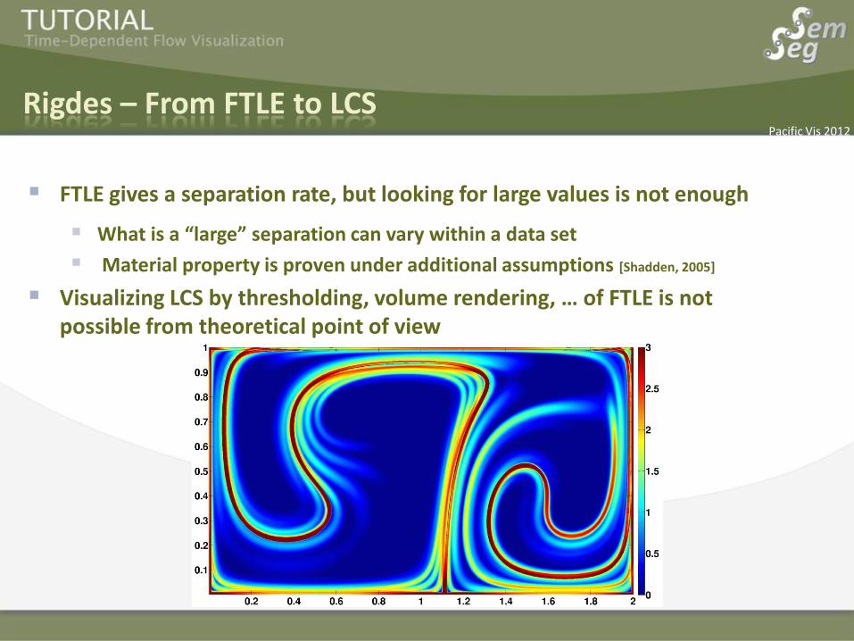
FTLE gives a separation rate, but looking for large values is not enough
What is a “large” separation can vary within a data set
Material property is proven under additional assumptions [Shadden, 2005]
Visualizing LCS by thresholding, volume rendering, … of FTLE is not possible from theoretical point of view
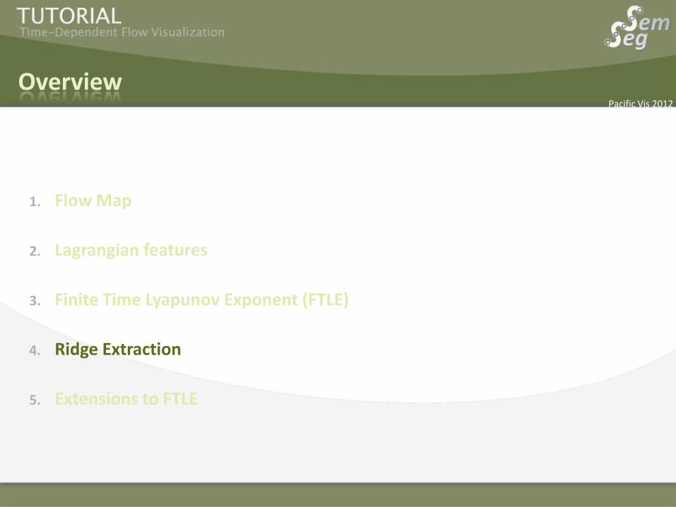
Rigdes – From FTLE to LCS
Pacific Vis 2012
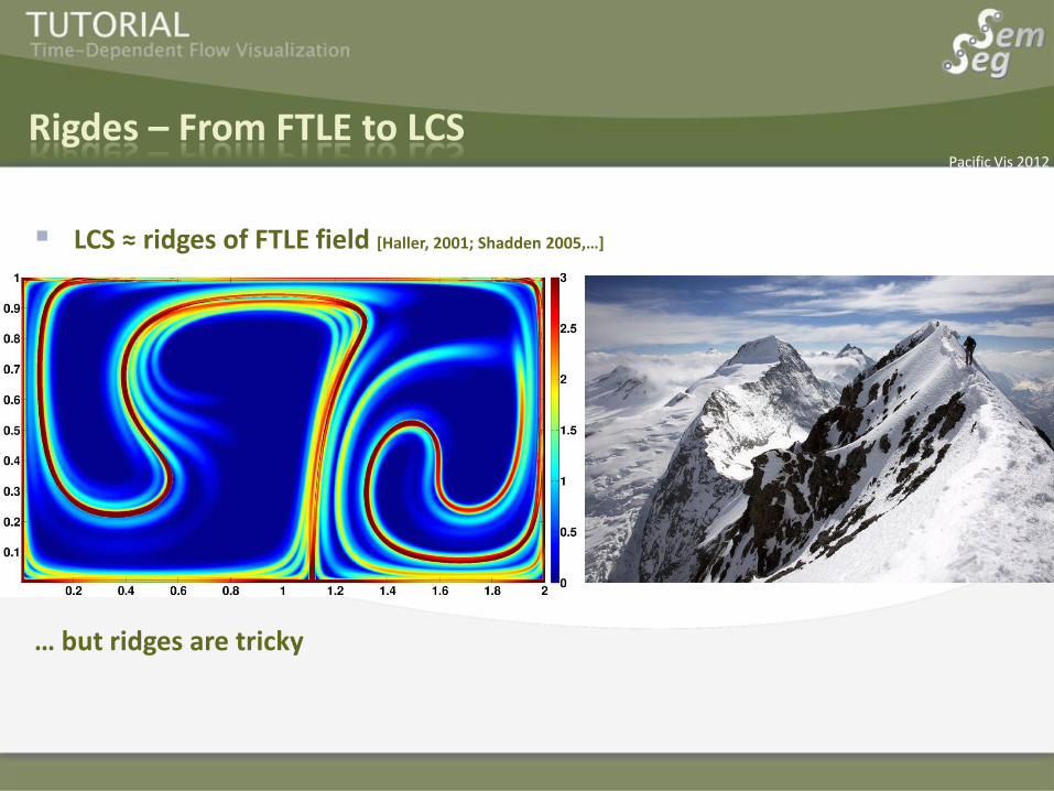
LCS ≈ ridges of FTLE field [Haller, 2001; Shadden 2005,…]
… but ridges are tricky
Rigdes – From FTLE to LCS
Pacific Vis 2012
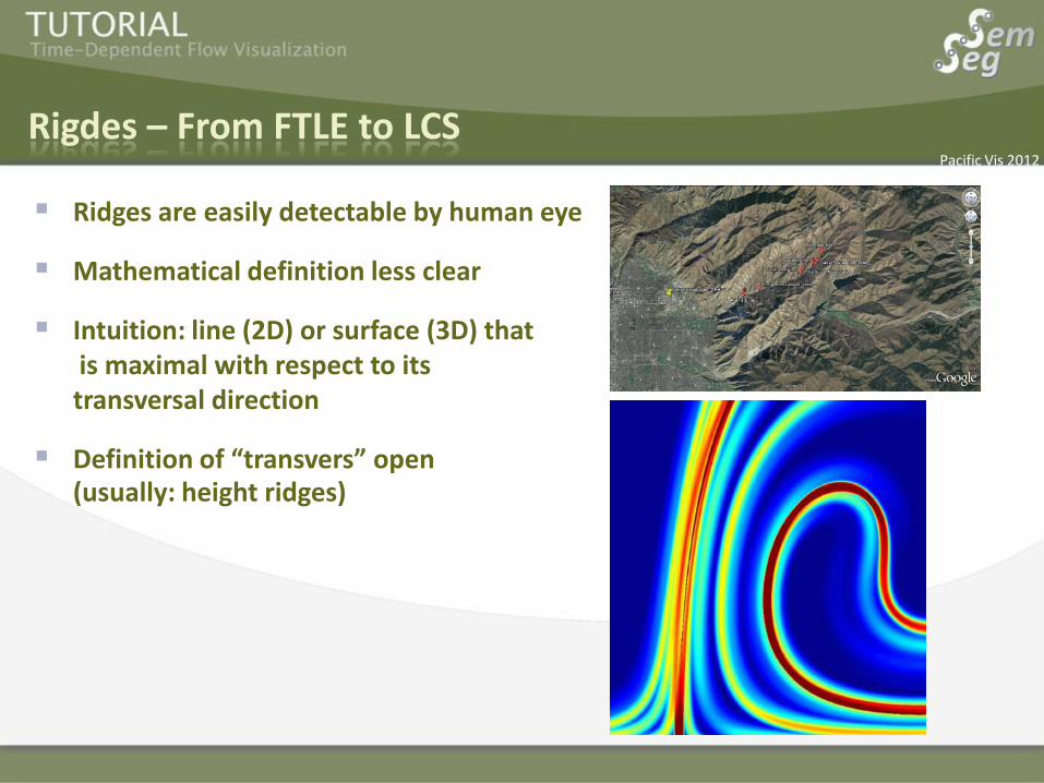
Ridges are easily detectable by human eye
Mathematical definition less clear
Intuition: line (2D) or surface (3D) that is maximal with respect to its transversal direction
Definition of “transvers” open (usually: height ridges)
Rigdes – From FTLE to LCS
Pacific Vis 2012
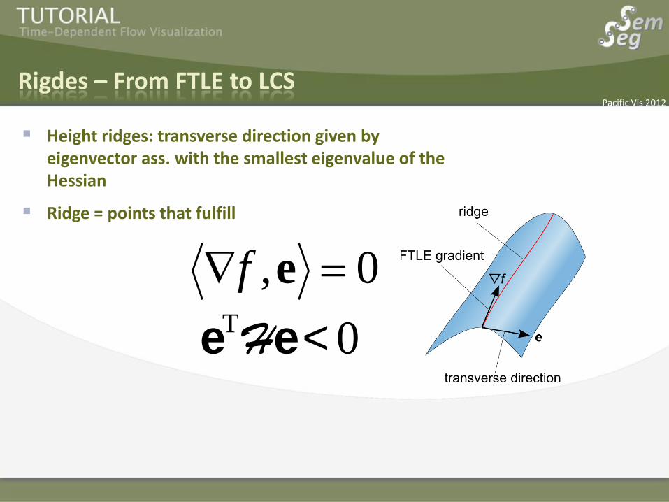
Height ridges: transverse direction given by eigenvector ass. with the smallest eigenvalue of the Hessian
Ridge = points that fulfill
Rigdes – From FTLE to LCS
0, ef
eTHe< 0
Pacific Vis 2012
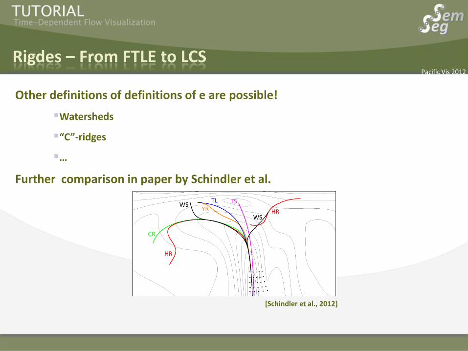
Other definitions of definitions of e are possible!
Watersheds
“C”-ridges
…
Further comparison in paper by Schindler et al.
Rigdes – From FTLE to LCS
[Schindler et al., 2012]
Pacific Vis 2012
High quality FTLE ridges…
Require dense seeding of particles
accurate integration scheme
… are computationally expensive!
Number of path lines + integration are main bottle neck in FTLE computation
Has to be done in precomputation step
Current state of the art: interactive computation not possible
Efficient FTLE computation
Timing for 2D FTLE on a regular grid (5122) [Hlawatsch et al., 2011]
Pacific Vis 2012
Some examples for simulated flow scenarios [Wasberg et al., 2009]
112 x 113 x 112 [Wasberg et al., 2009] Re=180
128 x 129 x 128 [Moser et al., 1999] Re=180
1536 x 257 x 1536 [del Alamo and Jimenez, 2003] Re=550
3072 x 385 x 2304 [del Alamo et al., 2004] Re=950
Typical Reynolds numbers: Blood flow in aorta ca 1000, large ships ca 5 x 10⁹ [Wikipedia]
For realistic scenarios efficient computation essential to be able to apply FTLE-based methods!
Timings in perspective…
Timing for 2D FTLE on a regular grid (5122) [Hlawatsch et al., 2011]
Pacific Vis 2012
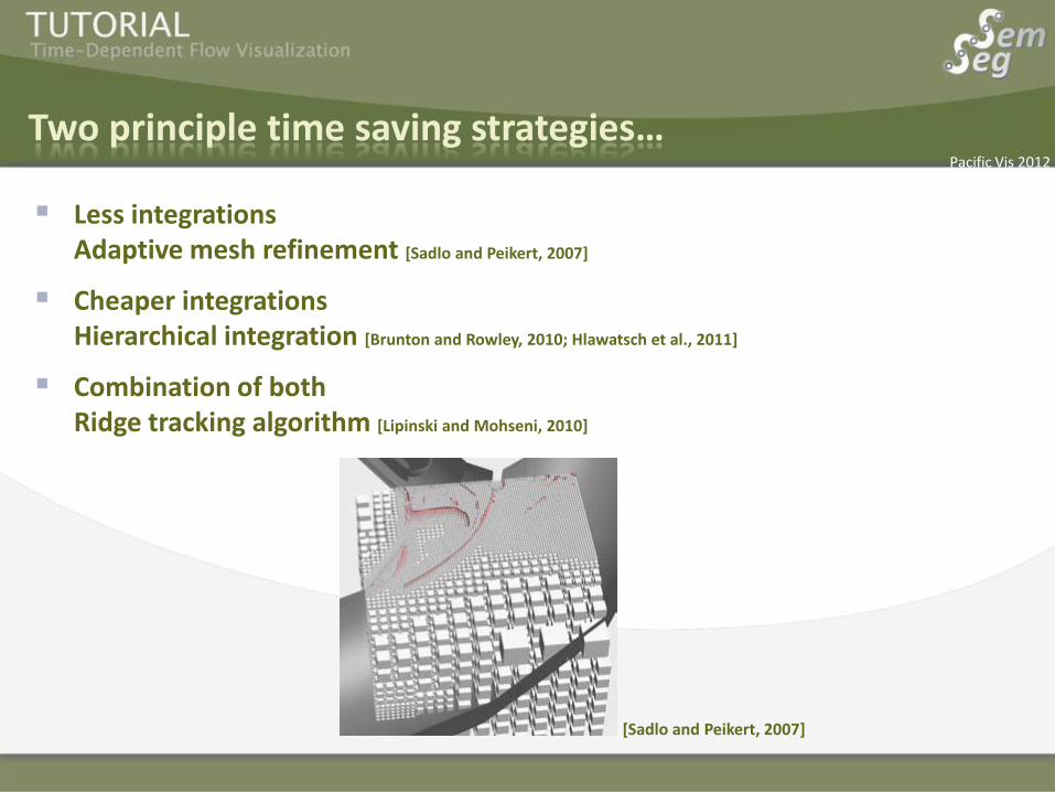
Less integrations Adaptive mesh refinement [Sadlo and Peikert, 2007]
Cheaper integrations Hierarchical integration [Brunton and Rowley, 2010; Hlawatsch et al., 2011]
Combination of both Ridge tracking algorithm [Lipinski and Mohseni, 2010]
Two principle time saving strategies…
[Sadlo and Peikert, 2007]
Pacific Vis 2012
Adaptive mesh refinement [Sadlo and Peikert, 2007]
Main loop: 1. Coarse seeding, pointwise verification of ridge
detection 2. Subdivision of detected ridge cells and neighbors 3. New pointwise ridge detection Pro and Cons: + Exact ridges - Relatively low speed-up (factor 4)
Pacific Vis 2012
Hierarchical Integration [Brunton and Rowley, 2010; Hlawatsch et al., 2011]
Main loop: 1. Integrate from each time step to next 2. Concatenate integration by interpolation Pro and Cons: + Large speed-up (factor 10) + Animations easily possible - Interpolation error
[Hlawatsch et al., 2011]
[Brunton and Rowley, 2010]
Pacific Vis 2012
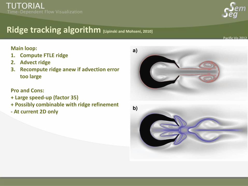
Ridge tracking algorithm [Lipinski and Mohseni, 2010]
Main loop: 1. Compute FTLE ridge 2. Advect ridge 3. Recompute ridge anew if advection error
too large Pro and Cons: + Large speed-up (factor 35) + Possibly combinable with ridge refinement - At current 2D only
Pacific Vis 2012
Thank you for your attention!
Tutorial: Time-Dependent Flow Visualization
The project SemSeg acknowledges the financial support of the Future and Emerging Technologies (FET) programme within the Seventh Framework Programme for Research of the European Commission, under FET-Open grant number 226042.
Armin Pobitzer1, Alexander Kuhn2
1) University of Bergen, Norway
2) University of Magdeburg, Germany
Pacific Vis 2012
Based on the following references:
A. Pobitzer, R. Peikert, R. Fuchs, B. Schindler, A. Kuhn, H. Theisel, K. Matkovic and H. Hauser
The State of the Art in Topology-Based Visualization of Unsteady Flow
Flow and Tensor Visualization Holger Theisel, University of Magdeburg, 2011
Flow Visualization Helwig Hauser, University of Bergen, 2011
Acknowledgements
The project SemSeg acknowledges the financial support of the Future and Emerging Technologies (FET) programme within the Seventh Framework Programme for Research of the European Commission, under FET-Open grant number 226042.
Pacific Vis 2012
[Laram2007] R. Laramee, H. Hauser, L. Zhao, and F. Post, Topology-based flow visualization, the state of the art Topology-based Methods in Visualization, 2007, p. 1–19.
[Haller2001] G. Haller, Lagrangian structures and the rate of strain in a partition of two-dimensional turbulence Physics of Fluids, vol. 13, 2001.
[Haller2010] G. Haller, A variational theory of hyperbolic Lagrangian Coherent Structures Physica D: Nonlinear Phenomena, vol. 240, Dec. 2010, pp. 574-598.
[Kasten2009] J. Kasten, C. Petz, I. Hotz, B.R. Noack, and H.-christian Hege, Localized finite-time Lyapunov exponent for unsteady flow analysis Vision Modeling and Visualization (VMV), vol. 1, 2009.
[Leung2011] S. Leung, An Eulerian Approach for Computing the Finite Time Lyapunov Exponent Journal of Computational Physics, Feb. 2011.
[Hlawa2010] M. Hlawatsch, F. Sadlo, and D. Weiskopf, Hierarchical Line Integration Transactions on Visualization and Computer Graphics, EEE, 2010.
[Sadlo2007] F. Sadlo and R. Peikert, Efficient visualization of lagrangian coherent structures by filtered AMR ridge extraction IEEE transactions on visualization and computer graphics, vol. 13, 2007, pp. 1456-63.
[Sadlo2009] F. Sadlo, A. Rigazzi, and R. Peikert, Time-Dependent Visualization of Lagrangian Coherent Structures by Grid Advection Topological Data Analysis and Visualization: Theory, Algorithms and Applications, Springer, 2009.
[Nese1989] J.M. Nese Quantifying local predictability in phase space Physica D: Nonlinear Phenomena, vol. 35, 1989, p. 237–250.
Literature
Pacific Vis 2012
[Pobitz2009] A. Pobitzer, R. Peikert, R. Fuchs, B. Schindler, A. Kuhn, H. Theisel, K. Matkovic, and H. Hauser, On the way towards topology-based visualization of unsteady flow-the state of the art IEEE Transactions on Visualization and Computer Graphics (Proceedings Visualization 2009), vol. 15, 2009, p. 1243–1250.
[TW02] H. Theisel and T. Weinkauf. Vector field metrics based on distance measures of first order critical points Journal of WSCG, 10(3):121–128, 2002.
[TSH01] X. Tricoche, G. Scheuermann, and H. Hagen. Continuous topology simplification of planar vector fields In Proc. of IEEE Visualization 2001, pages 159–166, 2001.
[TRS03] H. Theisel, Ch. Rössl, and H.-P. Seidel. Compression of 2D vector fields under guaranteed topology preservation Computer Graphics Forum (Eurographics 2003), 22(3):333–342, 2003.
[ZZ08] Zhonglin Zhang Identification of Lagrangian coherent structures around swimming jellyfish from experimental time-series data California Inst. of Technology, 2008
[WH10] W. Tang and P. W. Chan and G. Haller Accurate extraction of LCS over finite domains with application to flight data analysis over Hong Kong Int. Airport Chaos (Woodbury, N.Y.), 2010
[WTHS04] T.Weinkauf, H. Theisel, H.-C. Hege, and H.-P. Seidel. Topological construction and visualization of higher order 3D vector fields Computer Graphics Forum (Eurographics 2004), 23(3):469–478, 2004.
[Shadden06] Shawn C. Shadden, John O. Dabiri, and Jerrold E. Marsden. Lagrangian analysis of fluid transport in empirical vortex ring flows Physics of Fluids, 18(4):047105, 2006.
[Eberly96] D. Eberly. Ridges in Image and Data Analysis Kluwer Acadamic Publishers, Dordrecht, 1996.
Pacific Vis 2012
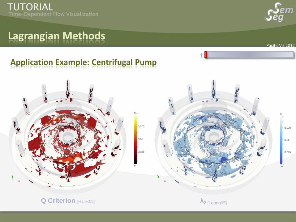
[Leong95] Jeong, J., Hussain, F. On the identification of a vortex Journal of Fluid Mechanics, Vol 285, pp 69 – 94, 1995
[Haller05] G. Haller, 2005 An objective definition of a vortex J. Fluid Mech., Vol. 525, pp 1-26, 2005
[Lucius10] A. Lucius, G.Brenner, Unsteady CFD simulations of a pump in part load conditions using Scale-Adaptive Simulation International Journal of Heat and Fluid Flow, Vol. 31 2010, pp 1113-1118
[Lucius10] A. Lucius, G. Brenner, Numerical simulation and evaluation of velocity fluctuations during rotating stall of a centrifugal pump Journal of Fluids Engineering Vol. 133 2011, pp 081102
[GaVIS2007] Garth, C., Gerhardt, F., Tricoche, X., and Hagen, H. Efficient computation and visualization of coherent structures in fluid flow applications IEEE transactions on visualization and computer graphics, vol. 13, 2007
[Garth2007] Garth C. et al. Visualization of Coherent Structures in 2D transient flows Topology-based Methods in Visualization, 2007, p. 1–19.
[Haller2005] G. Haller. An objective definition of a vortex Journal of Fluid Mechanics, 525:1–26, Feb. 2005.
[Jeong1995] J. Jeong. On the identification of a vortex Journal of Fluid Mechanics,285:69–94, 1995.
[Wein2007] T. Weinkauf, J. Sahner, H. Theisel, H.-C. Hege, and S. H.-P. Cores of swirling particle motion in unsteady flows IEEE Transactions onVisualization and Computer Graphics, 13(6):1759–1766, 2007.
Pacific Vis 2012
[Germer2011] T. Germer, M. Otto, R. Peikert and H. Theisel Lagrangian Coherent Structures with Guaranteed Material Separation Computer Graphics Forum (Proc. EuroVis), 2011
[Salz2008] Tobias Salzbrunn, Christoph Garth, Gerik Scheuermann und Joerg Meyer Pathline predicates and unsteady flow structures THE VISUAL COMPUTER, Volume 24, Number 12, 1039-1051
[Fuchs2010] R. Fuchs, J. Kemmler, B. Schindler, F. Sadlo, H. Hauser, R. Peikert, Toward a Lagrangian Vector Field Topology, Computer Graphics Forum, 29(3), pp. 1163-1172, 2010.
[Otto2011] M. Otto, A. Kuhn, W. Engelke and H. Theisel 2011 IEEE Visualization Contest Winner: Visualizing Unsteady Vortical Behavior of a Centrifugal Pump IEEE, Visualization Viewpoints in IEEE CG&A, Computer Graphics and Applications, 2012
[Haller, 2001] Haller, G., Lagrangian structures and the rate of strain in a partition of two-dimensional turbulence, Physics of Fluids, vol. 13, 2001
[Hlawatsch et al., 2010] Hlawatsch, M., Sadlo, F., Weiskopf, D., Hierarchical Line Integration, Transactions on Visualization and Computer Graphics, EEE, 2010.
[Sadlo and Peikert, 2007] Sadlo, F., Peikert, R., Efficient visualization of lagrangian coherent structures by filtered AMR ridge extraction, IEEE transactions on visualization and computer graphics, vol. 13, 2007, pp. 1456-63.
[Shadden et al., 2005] Shadden, S. C., Lekien, F., Marsden, J. E., Lagrangian analysis of fluid transport in empirical vortex ring flows, Physics of Fluids Vol 18, 047105, 2006.
[Wasberg et a., 2009] Wasberg, C. E., Gjesdal, T., Reif, B. A. P., Andreassen, Ø., Variational multiscale turbulence modelling in a
high order spectral element method, J. of Computational Physics Vol. 228, pp 7333–7356, 2009
[Brunton and Rowley, 2010] Brunton, S. L., Rowley, Fast Computations of finite-time Lyapunov exponent fields for unsteady flow, Chaos Vol. 20, 2010
[ Lipinski and Mohseni, 2010] Lipinski, D., Mohseni, K., A ridge tracking algorithm and error estimate for efficient computations of Lagrangian coherent structures, Chaos Vol. 20, 2010