58
Part 3 Measurements and Models for Traffic Engineering
| Date post: | 22-Dec-2015 |
| Category: |
Documents |
| View: | 213 times |
| Download: | 0 times |

Part 3
Measurements and Models
for Traffic Engineering

Traffic Engineering
• Goal: domain-wide control & management to– Satisfy performance goals– Use resources efficiently
• Knobs:– Configuration & topology: provisioning, capacity
planning– Routing: OSPF weights, MPLS tunnels, BGP
policies,…– Traffic classification (diffserv), admission control,
…
• Measurements are key: closed control loop– Understand current state, load, and traffic flow– Ask what-if questions to decide on control actions– Inherently coarse-grained

End-to-End Traffic & Demand Models
path matrix = bytes per path
demand matrix =bytes per source-destination pair
Ideally, capturesall the information about the current network state and behavior
Ideally, capturesall the information that isinvariant with respect to the network state

Domain-Wide Traffic & Demand Models
current state &traffic flow
fine grained:path matrix = bytes per path
intradomain focus:traffic matrix =bytes per ingress-egress
interdomain focus:demand matrix =bytes per ingress andset of possible egresses
predictedcontrol action:impact of intra-domain routing
predictedcontrol action:impact of inter-domain routing

Traffic Representations• Network-wide views
– Not directly supported by IP (stateless, decentralized)– Combining elementary measurements: traffic, topology,
state, performance– Other dimensions: time & time-scale, traffic class, source
or destination prefix, TCP port number
• Challenges– Volume– Lost & faulty measurements– Incompatibilities across types of measurements, vendors– Timing inconsistencies
• Goal– Illustrate how to populate these models: data analysis and
inference– Discuss recent proposals for new types of measurements

Outline
• Path matrix– Trajectory sampling– IP traceback
• Traffic matrix– Network tomography
• Demand matrix– Combining flow and routing data

Path Matrix: Operational Uses
• Congested link– Problem: easy to detect, hard to diagnose– Which traffic is responsible?– Which customers are affected?
• Customer complaint– Problem: customer has insufficient visibility to
diagnose – How is the traffic of a given customer routed?– Where does it experience loss & delay?
• Denial-of-service attack– Problem: spoofed source address, distributed
attack– Where is it coming from?

Path Matrix
• Bytes/sec for every path P between every ingress-egress pair
• Path matrix traffic matrix

Measuring the Path Matrix
• Path marking– Packets carry the path they have traversed– Drawback: excessive overhead
• Packet or flow measurement on every link– Combine records to obtain paths– Drawback: excessive overhead, difficulties in
matching up flows
• Combining packet/flow measurements with network state– Measurements over cut set (e.g., all ingress routers)– Dump network state– Map measurements onto current topology

Path Matrix through Indirect Measurement
• Ingress measurements + network state

Network State Uncertainty
• Hard to get an up-to-date snapshot of…• …routing
– Large state space– Vendor-specific implementation– Deliberate randomness– Multicast
• …element states– Links, cards, protocols,…– Difficult to infer
• …element performance– Packet loss, delay at links

Trajectory Sampling• Goal: direct observation
– No network model & state estimation
• Basic idea #1:– Sample packets at each link– Would like to either sample a packet everywhere or nowhere
– Cannot carry a « sample/don’t sample » flag with the packet
– Sampling decision based on hash over packet content– Consistent sampling trajectories
• x: subset of packet bits, represented as binary number• h(x) = x mod A• sample if h(x) < r• r/A: thinning factor
• Exploit entropy in packet content to obtain statistically representative set of trajectories

Fields Included in Hashes

Labeling
• Basic idea #2:– Do not need entire packet to reconstruct
trajectory– Packet identifier: computed through
second hash function g(x)– Observation: small labels (20-30 bits) are
sufficient to avoid collisions

Sampling and Labeling
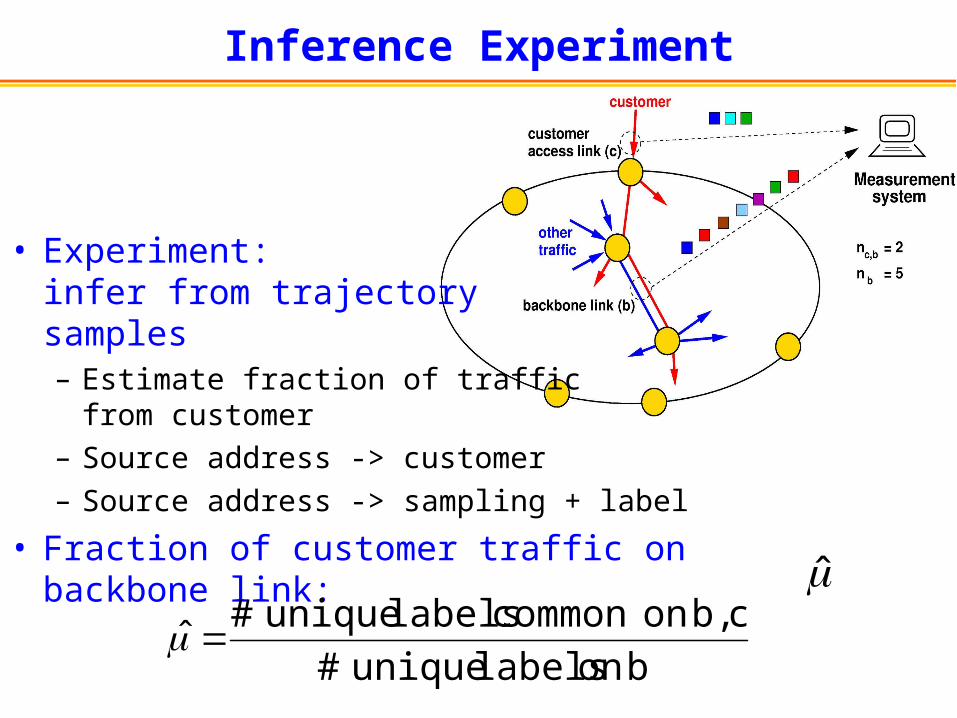
Inference Experiment
• Experiment: infer from trajectorysamples– Estimate fraction of traffic
from customer– Source address -> customer– Source address -> sampling + label
• Fraction of customer traffic on backbone link:
b on labels unique #cb, on common labels unique #

Estimated Fraction (c=1000bit)
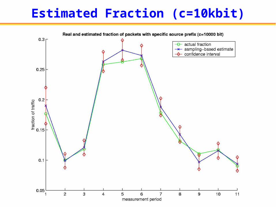
Estimated Fraction (c=10kbit)

Sampling Device

Trajectory Sampling: Summary
• Advantages– Trajectory sampling estimates path matrix
…and other metrics: loss, link delay– Direct observation: no routing model +
network state estimation– Can handle multicast traffic (source tree),
spoofed source addresses (denial-of-service attacks)
– Control over measurement overhead
• Disadvantages– Requires support on linecards

IP Traceback against DDoS Attacks
spoofed IPsource addresses
• Denial-of-service attacks– Overload victim with bogus traffic– Distributed DoS: attack traffic from large # of
sources– Source addresses spoofed to evade detection
cannot use traceroute, nslookup, etc.– Rely on partial path matrix to determine attack path

IP Traceback: General Idea
• Goal:– Find where traffic is really originating, despite spoofed
source addresses– Interdomain, end-to-end: victim can infer entire tree
• Crude solution– Intermediate routers attach their addresses to packets– Infer entire sink tree from attacking sources– Impractical:
• routers need to touch all the packets• traffic overhead
• IP Traceback: reconstruct tree from samples of intermediate routers– A packet samples intermediate nodes– Victim reconstructs attack path(s) from multiple
samples

IP Traceback: Node Sampling
• Router address field reserved in packet– Each intermediate router flips coin & records its
address in field with probability p
• Problems:– p<0.5: spoofed router field by attacker wrong path– p>0.5: hard to infer long paths– Cannot handle multiple attackers
A
B
C
A
A C
C
B
attacker
inter-mediaterouters
victim
A: 239B: 493C: 734
histogramof nodefrequencies
decreasingfrequency
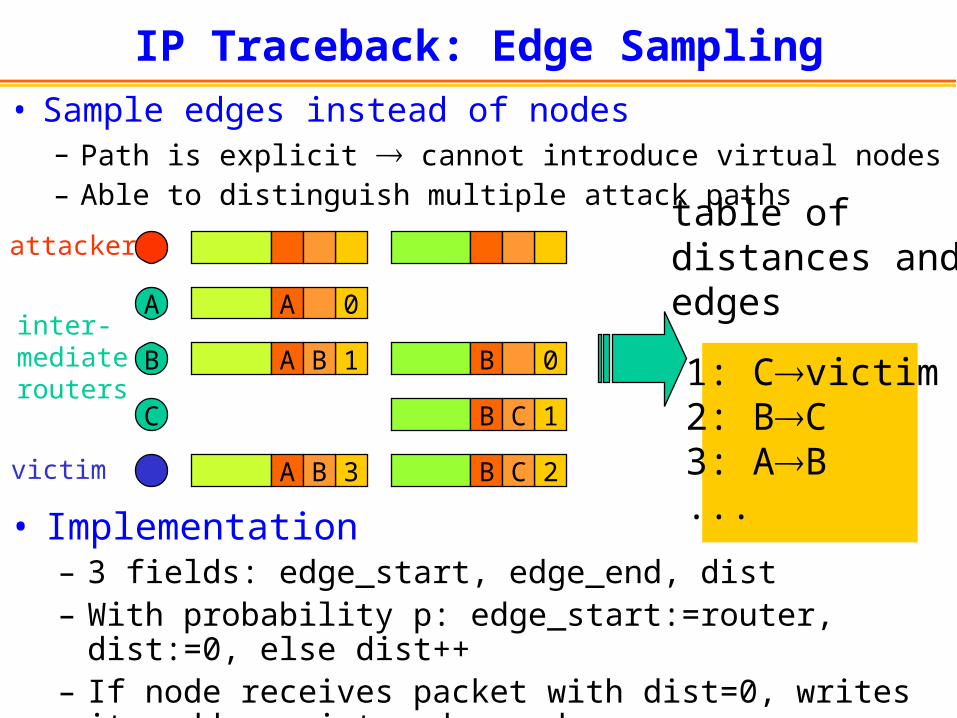
IP Traceback: Edge Sampling
• Sample edges instead of nodes– Path is explicit cannot introduce virtual nodes– Able to distinguish multiple attack paths
A
B
C
A
A B
attacker
inter-mediaterouters
victim
1: Cvictim2: BC3: AB...
table ofdistances andedges
• Implementation– 3 fields: edge_start, edge_end, dist– With probability p: edge_start:=router, dist:=0, else
dist++– If node receives packet with dist=0, writes its
address into edge_end
0
3B
A 1B
2C
B 0
B 1C

IP Traceback: Compressed Edge Sampling
• Avoid modifying packet header– Identification field: only used for
fragmentation– Overload to contain compressed edge
samples
• Three key ideas:– Both_edges := edge_start xor edge_end– Fragment both_edges into small pieces– Checksum to avoid combining wrong pieces
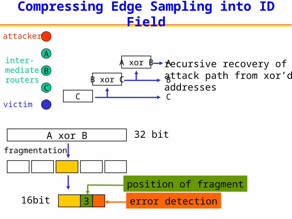
Compressing Edge Sampling into ID Field
A
B
C
attacker
inter-mediaterouters
victim
A xor B
B xor C
C C
B
A recursive recovery ofattack path from xor’daddresses
A xor B
fragmentation
32 bit
3
position of fragment
error detection16bit

IP Traceback: Summary
• Interdomain and end-to-end– Victim can infer attack sink tree from sampled
topology information contained in packets– Elegantly exploits basic property of DoS attack:
large # of samples
• Limitations– ISPs implicitly reveal topology– Overloading the id field: makes fragmentation
impossible, precludes other uses of id field• other proposed approach uses out-of-band ICMP packets
to transport samples
• Related approach: hash-based IP traceback– “distributed trajectory sampling”, where trajectory
reconstruction occurs on demand from local information

Path Matrix: Summary
• Changing routers vs. changing IP– Both trajectory sampling and IP traceback require
router support– This is hard, but easier than changing IP!– If IP could be changed:
• trajectory sampling: sample-this-packet bit, coin flip at ingress
• IP traceback: reserved field for router sampling
– Tricks to fit into existing IP standard• trajectory sampling: consistent sampling by hashing over
packet• IP traceback: edge sampling, compression, error correction
• Direct observation– No joining with routing information– No router state

Outline
• Path matrix– Trajectory sampling– IP traceback
• Traffic matrix– Network tomography
• Demand matrix– Combining flow and routing data

Traffic Matrix: Operational Uses
• Short-term congestion and performance problems– Problem: predicting link loads and performance after a
routing change– Map traffic matrix onto new routes
• Long-term congestion and performance problems– Problem: predicting link loads and performance after
changes in capacity and network topology– Map traffic matrix onto new topology
• Reliability despite equipment failures– Problem: allocating sufficient spare capacity after likely
failure scenarios– Find set of link weights such that no failure scenario
leads to overload (e.g., for “gold” traffic)

Obtaining the Traffic Matrix
• Full MPLS mesh:– MPLS MIB per LSP– Establish a separate LSP for every ingress-egress
point
• Packet monitoring/flow measurement with routing– Measure at ingress, infer egress (or vice versa)– Last section
• Tomography:– Assumption: routing is known (paths between
ingress-egress points)– Input: multiple measurements of link load (e.g., from
SNMP interface group)– Output: statistically inferred traffic matrix

4Mbps 4Mbps
3Mbps5Mbps
Network Tomography
Origins
Destinations
From link counts to the traffic matrix

cdy
111
111
1111
1
1111
111
1
A
Matrix Representation
c
a
b d
Axy counts link:),...,( T
ryyy 1
counts OD:),...,( Tcxxx 1
adx

Single Observation is Insufficient
• Linear system is underdetermined– Number of links– Number of OD pairs– Dimension of solution sub-space at
least
• Multiple observations are needed– Stochastic model to bind them
)(nOr )( 2nOc
rc

Network Tomography
• [Y. Vardi, Network Tomography, JASA, March 1996]
• Inspired by road traffic networks, medical tomography
• Assumptions:– OD counts:– OD counts independent & identically
distributed (i.i.d.)– K independent observations
))(jPoisson(k
jX
)()1( ,..., KYY

Vardi Model: Identifiability
• Model: parameter , observation• Identifiability: determines
uniquely – Theorem: If the columns of A are all
distinct and non-zero, then is identifiable.
– This holds for all “sensible” networks– Necessary is obvious, sufficient is not
)(Yp
Y

Maximum Likelihood Estimator
• Likelihood function:
• Difficulty: determining • Maximum likelihood estimate
– May lie on boundary of – Iterative methods (such as EM) do not
always converge to correct estimate
AXYXXPYPL
:)()()(
}0,:{ XYAXX
}:{ YAXX

Estimator Based on Method of Moments
• Gaussian approximation of sample mean
• Match mean+covariance of model to sample mean+covariance of observation
• Mean:• Cross-covariance:
AYAXY ˆ
Tji
Tjiji
AdiagAYY
AXXAYY
)(),v(oc
),cov(),cov(

• Linear estimating eq:
• System inconsistent + overconstrained– Inconsistent: e.g.,– Overconstrained:
– Massage eqn system, LININPOS problem
Linear Estimation
K
k
k AYK
Y1
)(1ˆ
Tji
kj
K
k
kijiij AdiagAYYYYYYS
)(ˆˆ),v(oc )(
1
)(
B
A
S
Y
2iii YS
crr
BcrA
2
)1(:;:

How Well does it Work?
• Experiment [Vardi]:– K=100
• Limitations:– Poisson traffic– Small network
c
a
b d
14.12
33.11
87.9
25.9
92.7
84.6
79.5
06.5
72.4
68.2
37.2
01.1
ˆ,
12
11
10
9
8
7
6
5
4
3
2
1
EX

Further Papers on Tomography
• [J. Cao et al., Time-Varying Network Tomography, JASA, Dec 2000]– Gaussian traffic model, mean-variance
scaling
• [Tebaldi & West, Bayesian Inference on Network Traffic…, JASA, June 1998]– Single observation, Bayesian prior
• [J. Cao et al., Scalable Method…, submitted, 2001]– Heuristics for efficient computation

Open Questions & Research Problems
• Precision– Vardi: traffic generated by model, large # of
samples– Nevertheless significant error!
• Scalability to large networks– Partial queries over subgraphs
• Realistic traffic models– Cannot handle loss, multicast traffic– Marginals:Poisson & Gaussian– Dependence of OD traffic intensity– Adaptive traffic (TCP)– Packet loss
• How to include partial information– Flow measurements, packet sampling

Outline
• Path matrix– Trajectory sampling– IP traceback
• Traffic matrix– Network tomography
• Demand matrix– Combining flow and routing data
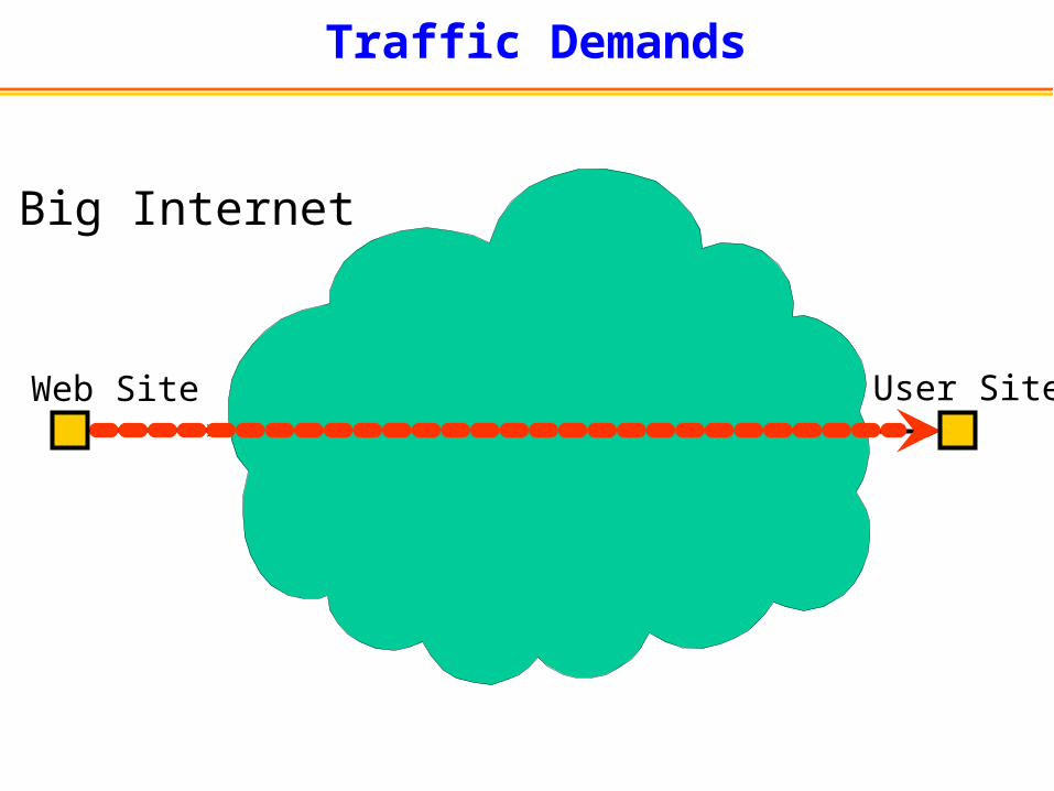
Traffic Demands
Big Internet
Web Site User Site

Coupling between Inter and Intradomain
Web Site User Site
AS 1AS 3
AS 4
U
AS 3, U
AS 3, U
AS 3, U
• IP routing: first interdomain path (BGP), then determine intradomain path (OSPF,IS-IS)
AS 4, AS 3, U
AS 2

Intradomain Routing
Zoom in on AS1
200
11010
110
300
25
75
50
300
IN
OUT 2
110
• Change in internal routing configuration changes flow exit point!(hot-potato routing)
110
OUT 3
OUT 1

Demand Model: Operational Uses
• Coupling problem with traffic matrix-based approach:
– traffic matrix changes after changing intradomain routing!
• Definition of demand matrix: # bytes for every(in, {out_1,...,out_m})– ingress link (in)– set of possible egress links ({out_1,...,out_m})
Traffic matrix
Traffic Engineering
Improved Routing
Traffic matrix
Traffic Engineering
Improved Routing
Demand matrix
Traffic Engineering
Improved Routing

Ideal Measurement Methodology
• Measure traffic where it enters the network– Input link, destination address, # bytes, and
time– Flow-level measurement (Cisco NetFlow)
• Determine where traffic can leave the network– Set of egress links associated with each
destination address (forwarding tables)
• Compute traffic demands– Associate each measurement with a set of
egress links
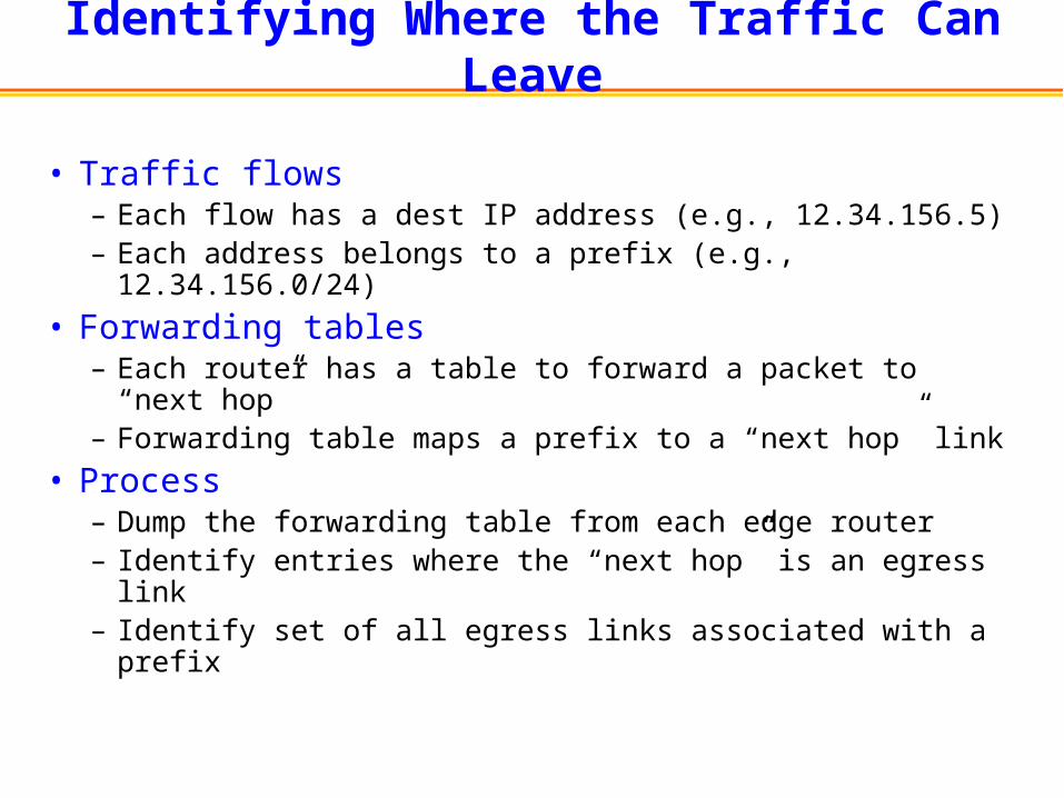
Identifying Where the Traffic Can Leave
• Traffic flows– Each flow has a dest IP address (e.g., 12.34.156.5)– Each address belongs to a prefix (e.g., 12.34.156.0/24)
• Forwarding tables– Each router has a table to forward a packet to “next
hop”– Forwarding table maps a prefix to a “next hop” link
• Process– Dump the forwarding table from each edge router– Identify entries where the “next hop” is an egress link– Identify set of all egress links associated with a prefix

Identifying Egress Links
Flow->12.34.156.5
A
Forwarding entry: 12.34.156.5/24x

Case Study: Interdomain Focus
• Not all links are created equal: access vs. peering– Access links:
• large number, diverse• frequent changes• burdened with other functions: access control, packet
marking, SLAs and billing...
– Peering links:• small number• stable
• Practical solution: measure at peering links only– Flow level measurements at peering links
• need both directions!
– A large fraction of the traffic is interdomain – Combine with reachability information from all routers

Inbound & Outbound Flows on Peering Links
Peers Customers
Inbound
Outbound
Note: Ideal methodology applies for inbound flows.
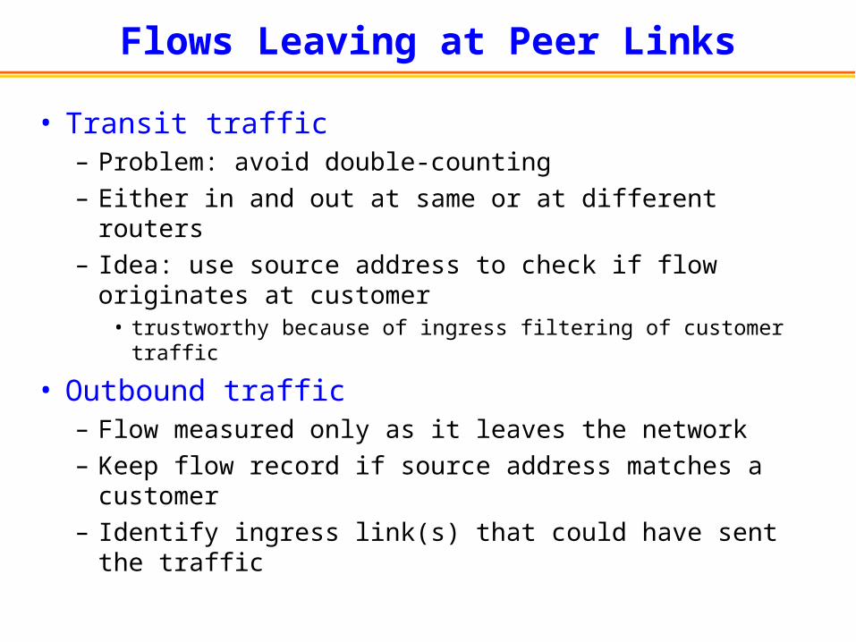
Flows Leaving at Peer Links
• Transit traffic– Problem: avoid double-counting– Either in and out at same or at different routers– Idea: use source address to check if flow
originates at customer• trustworthy because of ingress filtering of customer
traffic
• Outbound traffic– Flow measured only as it leaves the network– Keep flow record if source address matches a
customer– Identify ingress link(s) that could have sent the
traffic

Challenge: Ingress Links for Outbound
Use routing simulation to trace back to the ingress links -> egress links partition set of ingress links
? input
? input
Outbound traffic flowmeasured at peering link
Customersdestination
output

Experience with Populating the Model• Largely successful
– 98% of all traffic (bytes) associated with a set of egress links
– 95-99% of traffic consistent with an OSPF simulator
• Disambiguating outbound traffic– 67% of traffic associated with a single ingress link– 33% of traffic split across multiple ingress (typically, same
city!)
• Inbound and transit traffic (uses input measurement)– Results are good
• Outbound traffic (uses input disambiguation)– Results are pretty good, for traffic engineering
applications, but there are limitations– To improve results, may want to measure at selected or
sampled customer links

Open Questions & Research Problem
• Online collection of topology, reachability, & traffic data– Distributed collection for scalability
• Modeling the selection of the ingress link (e.g., use of multi-exit descriminator in BGP)– Multipoint-to-multipoint demand model
• Tuning BGP policies to the prevailing traffic demands

Traffic Engineering: Summary
• Traffic engineering requires domain-wide measurements + models– Path matrix (per-path): detection, diagnosis
of performance problems; denial-of-service attacks
– Traffic matrix (point-to-point): predict impact of changes in intra-domain routing & resource allocation; what-if analysis
– Demand matrix (point-to-multipoint): coupling between interdomain and intradomain routing: multiple potential egress points

Conclusion• IP networks are hard to measure by design
– Stateless and distributed– Multiple, competing feedback loops: users, TCP,
caching, content distribution networks, adaptive routing... difficult to predict impact of control actions
– Measurement support often an afterthought insufficient, immature, not standardized
• Network operations critically rely on measurements– Short time-scale: detect, diagnose, fix problems in
configuration, state, performance– Long time-scale: capacity & topology planning,
customer acquisition, ...
• There is much left to be done!– Instrumentation support; systems for collection &
analysis; procedures


