Page 1
Partial Differential Equations (PDEs)
classification groups
19
Source: [Farlow, 2012]
PDEs can be classified from different perspectives:
1. Order of PDE: The highest order of PDE
2. Number of variables: The number of independent variables for all
the involved functions:
Note: Under certain conditions when initial / boundary conditions and
partial derivatives are independent of a given variable we can reduce
the number of variables.
Page 2
Partial Differential Equations (PDEs)
classification groups
20 Source: [Farlow, 2012]
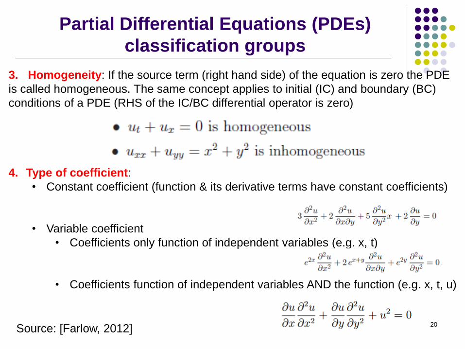
3. Homogeneity: If the source term (right hand side) of the equation is zero the PDE
is called homogeneous. The same concept applies to initial (IC) and boundary (BC)
conditions of a PDE (RHS of the IC/BC differential operator is zero)
4. Type of coefficient:
• Constant coefficient (function & its derivative terms have constant coefficients)
• Variable coefficient
• Coefficients only function of independent variables (e.g. x, t)
• Coefficients function of independent variables AND the function (e.g. x, t, u)
Page 3
Partial Differential Equations (PDEs)
classification groups
21 Source: [Farlow, 2012]
5. Hyperbolic / parabolic / elliptic PDEs:
- The classification becomes more clear in the next few slides. Below is the brief
description of some of their characteristics and sample applications.
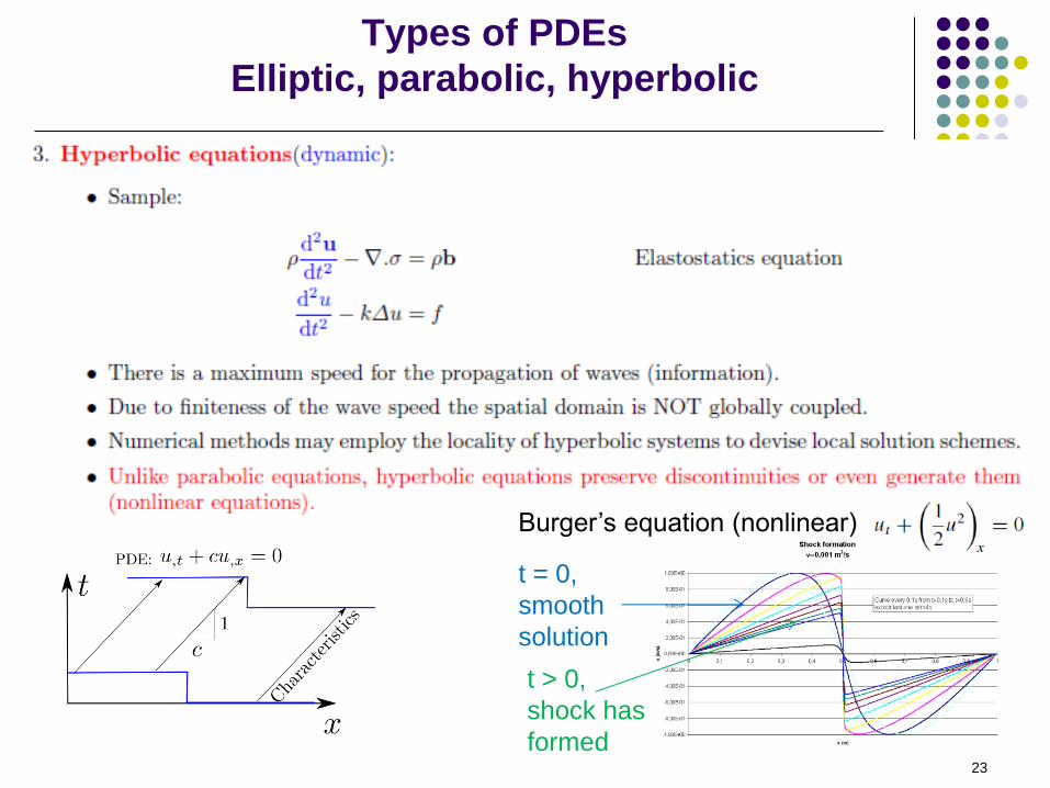
• Hyperbolic PDEs correspond to the propagation of waves and there is a
finite speed of propagation of waves. They tend to preserve or generate
discontinuities (in the absence of damping). Hyperbolic PDEs are often
transient although some steady-state limits of transient PDEs can be
hyperbolic as well (e.g. steady advection problems).
Examples: Elastodynamics, Transient electromagnetics; Acoustic equation.
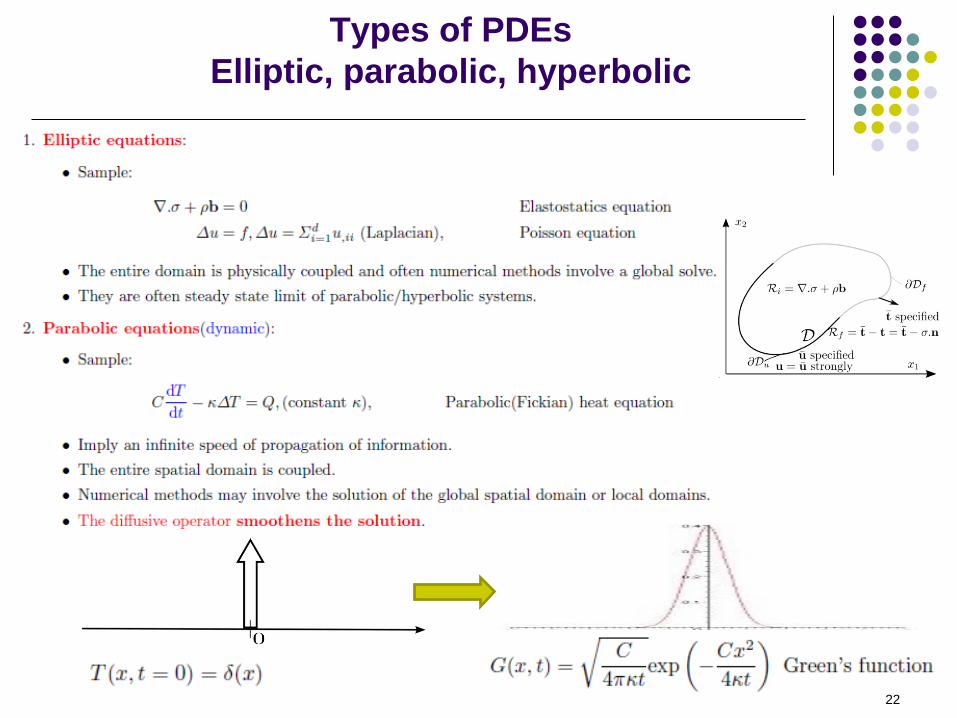
• Parabolic PDEs: Unlike hyperbolic PDEs the speed of propagation of
information is infinite for parabolic PDEs. They also tend to dissipate sharp
solution features and have a “diffusive” behavior. Many transient diffusion
problems are modeled (or idealized) by parabolic PDEs. Some examples are
Examples: Fourier heat equation; Viscous flow (Navier-Stokes equations)
• Elliptic PDEs: Elliptic problems are characterized by the global coupling of
the solution. They often correspond to steady-state limit of hyperbolic and
parabolic PDEs.
Page 4
Types of PDEs
Elliptic, parabolic, hyperbolic
22
Page 5
t = 0,
smooth
solution
t > 0,
shock has
formed
Burger’s equation (nonlinear)
23
Types of PDEs
Elliptic, parabolic, hyperbolic
Page 6
Partial Differential Equations (PDEs)
classification groups
24
Source: [Levandosky, 2002]
6. Linearity:
- The PDE is linear if the dependent variable and all its derivatives appear linearly in
the PDE. The nonlinear PDEs are classified into several groups as their solution
characteristics can be quite distinct:
Notations:
• Multi-index
• Multi-index partial derivative
example:
• Collection of all partial derivatives of order k:
example:
Page 7
Partial Differential Equations (PDEs)
llinear/nonlinear classifications
25
Source: [Levandosky, 2002]
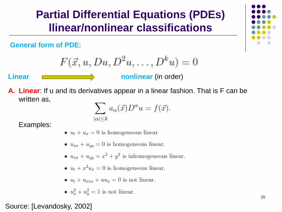
General form of PDE:
Linear nonlinear (in order)
A. Linear: If u and its derivatives appear in a linear fashion. That is F can be
written as,
Examples:
Page 8
Partial Differential Equations (PDEs)
llinear/nonlinear classifications
26
Source: [Levandosky, 2002]
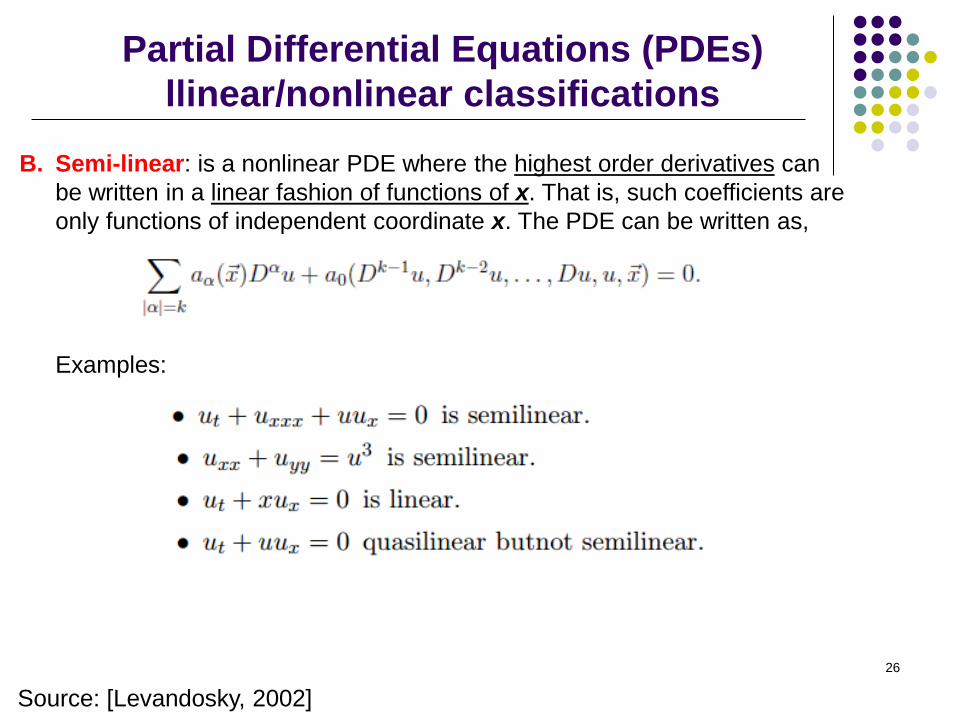
B. Semi-linear: is a nonlinear PDE where the highest order derivatives can
be written in a linear fashion of functions of x. That is, such coefficients are
only functions of independent coordinate x. The PDE can be written as,
Examples:
Page 9
Partial Differential Equations (PDEs)
llinear/nonlinear classifications
27
Source: [Levandosky, 2002]
C. Quasi-linear: is a nonlinear PDE, that is not semilinear and its highest
derivatives can be written as linear function of functions of x and lower
order derivatives of u. That is, it can be written as,
That is the coefficients of highest order terms depend on
Examples:
Is quasilinear
semilinear if a(x, y), b(x,y)
linear if a(x, y), b(x, y) and c = u d(x, y)
Page 10
Partial Differential Equations (PDEs)
llinear/nonlinear classifications
28
Source: [Levandosky, 2002]
D. Fully-nonlinear: If it’s nonlinear and cannot be written in quasi-linear,
semi-linear forms.
For a list of well-known nonlinear (semi-linear, quasi-linear, and fully nonlinear) PDEs refer to
here (https://en.wikipedia.org/wiki/List_of_nonlinear_partial_differential_equations)
Page 11
Partial Differential Equations (PDEs)
classification groups
29 Source: [Farlow, 2012]
• Semi-linear
• Quasi-linear
• Fully-nonlinear
Page 12
Solution to 1D wave equation
30 Source: [Farlow, 2012]
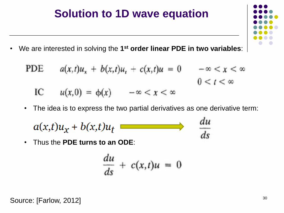
• We are interested in solving the 1st order linear PDE in two variables:
• The idea is to express the two partial derivatives as one derivative term:
• Thus the PDE turns to an ODE:
Page 13
Solution to 1D wave equation
31 Source: [Farlow, 2012]
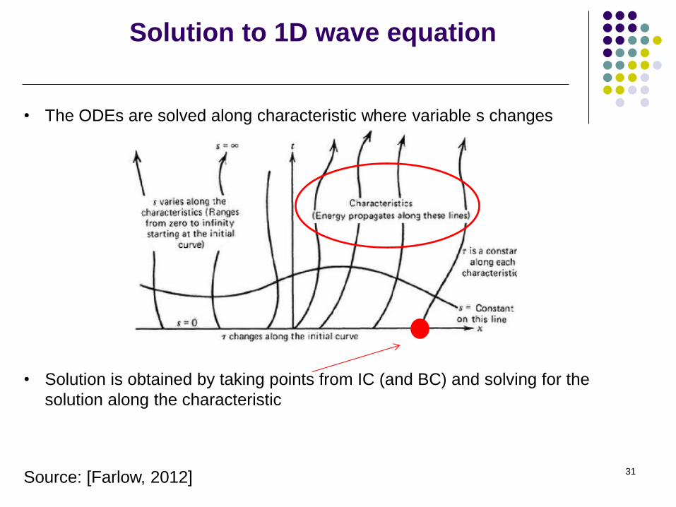
• The ODEs are solved along characteristic where variable s changes
• Solution is obtained by taking points from IC (and BC) and solving for the
solution along the characteristic
Page 14
Solution to 1D wave equation
32 Source: [Farlow, 2012]
• How this is done? By using the chain rule:
• The solution to ODEs provides the direction of characteristics
where x and t are obtained
from ODEs:
Page 15
Solution to 1D wave equation
Example: constant coefficients
33 Source: [Farlow, 2012]
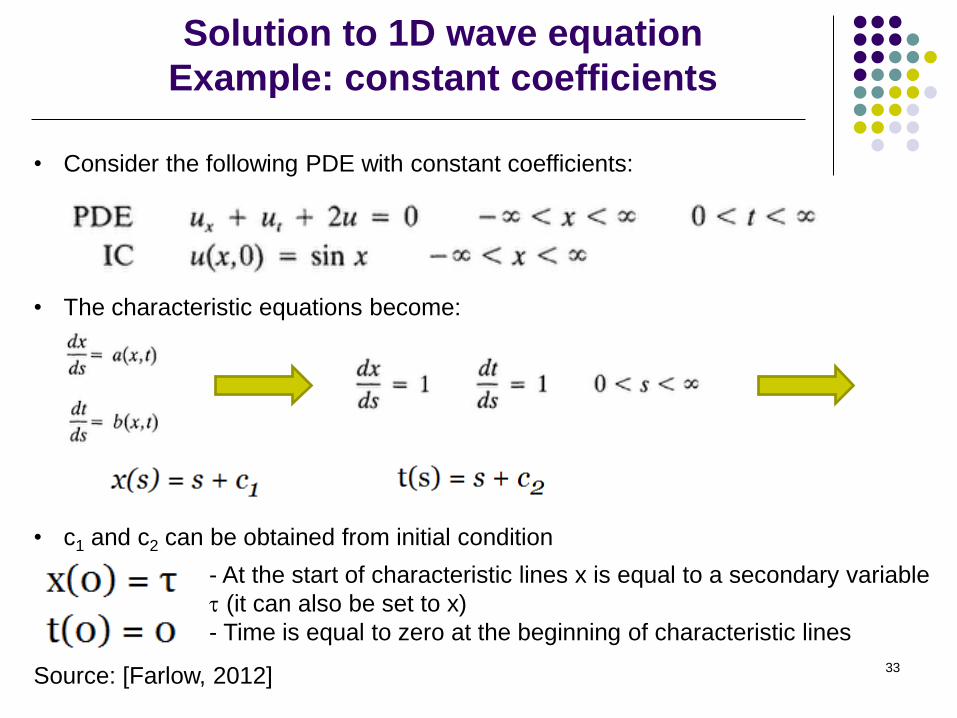
• Consider the following PDE with constant coefficients:
• The characteristic equations become:
• c1 and c2 can be obtained from initial condition
- At the start of characteristic lines x is equal to a secondary variable
t (it can also be set to x)
- Time is equal to zero at the beginning of characteristic lines
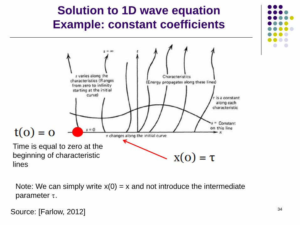
Page 16
Solution to 1D wave equation
Example: constant coefficients
34 Source: [Farlow, 2012]
Time is equal to zero at the
beginning of characteristic
lines
Note: We can simply write x(0) = x and not introduce the intermediate
parameter t.
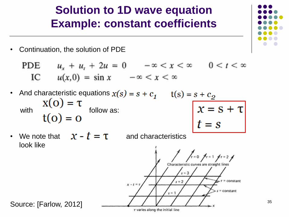
Page 17
Solution to 1D wave equation
Example: constant coefficients
35 Source: [Farlow, 2012]
• Continuation, the solution of PDE
• And characteristic equations
with follow as:
• We note that and characteristics
look like
Page 18
Solution to 1D wave equation
Example: constant coefficients
36 Source: [Farlow, 2012]
• Thus the PDE turns to the following ODE:
• Solving the Initial Value Problem (IVP) we get
• and by inverting (s, t) (x, t)
we get
• Thus becomes
Page 19
Solution to 1D wave equation
Example: constant coefficients
37 Source: [Farlow, 2012]
• So the solution to
Is
Which is a sine wave moving with speed 1 and damping in time
Page 20
Solution to 1D wave equation
Example: variable coefficients
38 Source: [Farlow, 2012]
• Consider the problem
• Step 1: The ODEs for characteristics are:
Hence
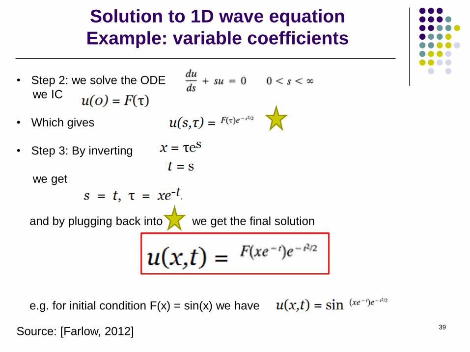
Page 21
Solution to 1D wave equation
Example: variable coefficients
39 Source: [Farlow, 2012]
• Step 2: we solve the ODE
we IC
• Which gives
• Step 3: By inverting
we get
and by plugging back into we get the final solution
e.g. for initial condition F(x) = sin(x) we have
Page 22
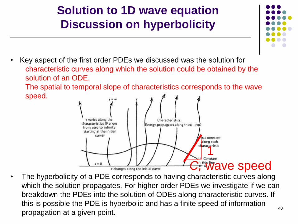
Solution to 1D wave equation
Discussion on hyperbolicity
40
• Key aspect of the first order PDEs we discussed was the solution for
characteristic curves along which the solution could be obtained by the
solution of an ODE.
The spatial to temporal slope of characteristics corresponds to the wave
speed.
• The hyperbolicity of a PDE corresponds to having characteristic curves along
which the solution propagates. For higher order PDEs we investigate if we can
breakdown the PDEs into the solution of ODEs along characteristic curves. If
this is possible the PDE is hyperbolic and has a finite speed of information
propagation at a given point.
C, wave speed
1
Page 23
Classification of second order PDEs:
Two independent parameters
41
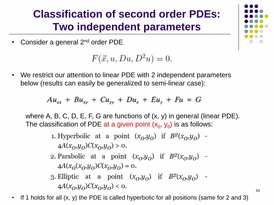
• Consider a general 2nd order PDE
• We restrict our attention to linear PDE with 2 independent parameters
below (results can easily be generalized to semi-linear case):
where A, B, C, D, E, F, G are functions of (x, y) in general (linear PDE).
The classification of PDE at a given point (x0, y0) is as follows:
• If 1 holds for all (x, y) the PDE is called hyperbolic for all positions (same for 2 and 3)
Page 24
Classification of second order PDEs:
Two independent parameters
42
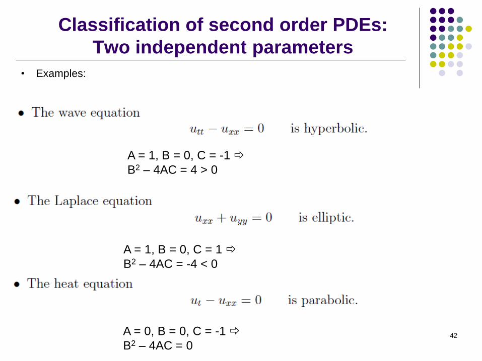
• Examples:
A = 1, B = 0, C = -1
B2 – 4AC = 4 > 0
A = 1, B = 0, C = 1
B2 – 4AC = -4 < 0
A = 0, B = 0, C = -1
B2 – 4AC = 0
Page 25
Classification of second order PDEs:
Canonical form
45
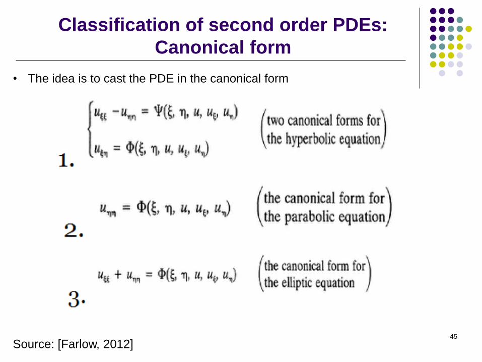
• The idea is to cast the PDE in the canonical form
Source: [Farlow, 2012]
Page 26
Classification of second order PDEs:
Canonical form
46
• We look for parameters x and h that cast the PDE into the hyperbolic form
• By transformation
• By change of parameters we obtain
Source: [Farlow, 2012]
Page 27
Classification of second order PDEs:
Canonical form
47
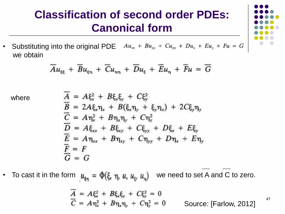
• Substituting into the original PDE
we obtain
where
• To cast it in the form we need to set A and C to zero.
Source: [Farlow, 2012]
Page 28
Classification of second order PDEs:
Canonical form
48
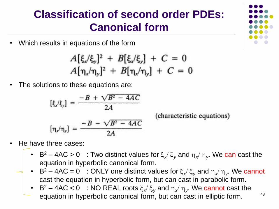
• Which results in equations of the form
• The solutions to these equations are:
• He have three cases:
• B2 – 4AC > 0 : Two distinct values for xx/ xy and hx/ hy. We can cast the
equation in hyperbolic canonical form.
• B2 – 4AC = 0 : ONLY one distinct values for xx/ xy and hx/ hy. We cannot
cast the equation in hyperbolic form, but can cast in parabolic form.
• B2 – 4AC < 0 : NO REAL roots xx/ xy and hx/ hy. We cannot cast the
equation in hyperbolic canonical form, but can cast in elliptic form.
Page 29
Classification of second order PDEs:
Characteristic values and curves
49
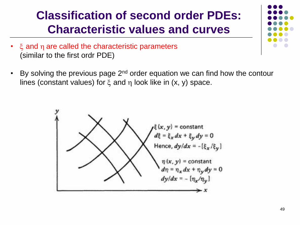
• x and h are called the characteristic parameters
(similar to the first ordr PDE)
• By solving the previous page 2nd order equation we can find how the contour
lines (constant values) for x and h look like in (x, y) space.
Page 30
Classification of second order PDEs:
Example
50
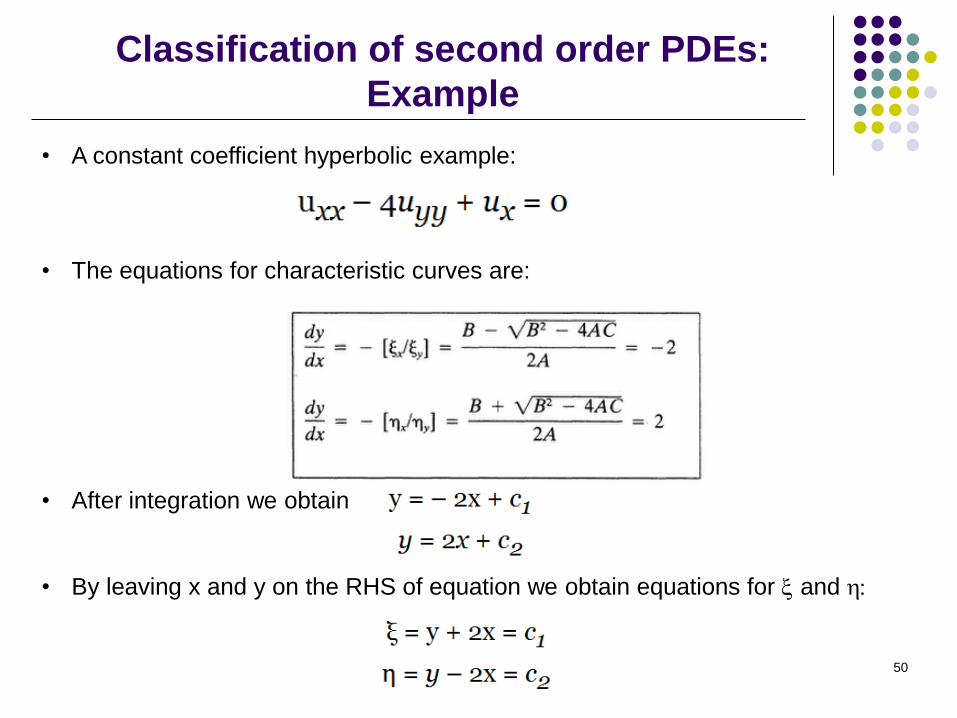
• A constant coefficient hyperbolic example:
• The equations for characteristic curves are:
• After integration we obtain
• By leaving x and y on the RHS of equation we obtain equations for x and h:
Page 31
Classification of second order PDEs:
Example
51
• And the characteristic curves look like
Page 32
Classification of second order PDEs:
Example with variable coefficients
52
• Consider the PDE
which is a hyperbolic equation in the first quadrant.
• We find the characteristics by the equation
• By solving these equations and moving x, y to the RHS we obtain
Page 33
Classification of second order PDEs:
Example with variable coefficients
53
• To obtain the form of the equation in the canonical form
we compute
where A and C are zero (why?)
Page 34
Classification of second order PDEs:
Example with variable coefficients
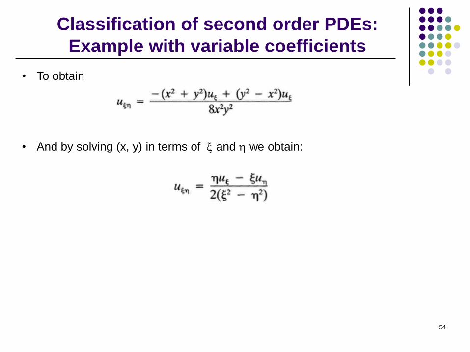
54
• To obtain
• And by solving (x, y) in terms of x and h we obtain:
Page 35
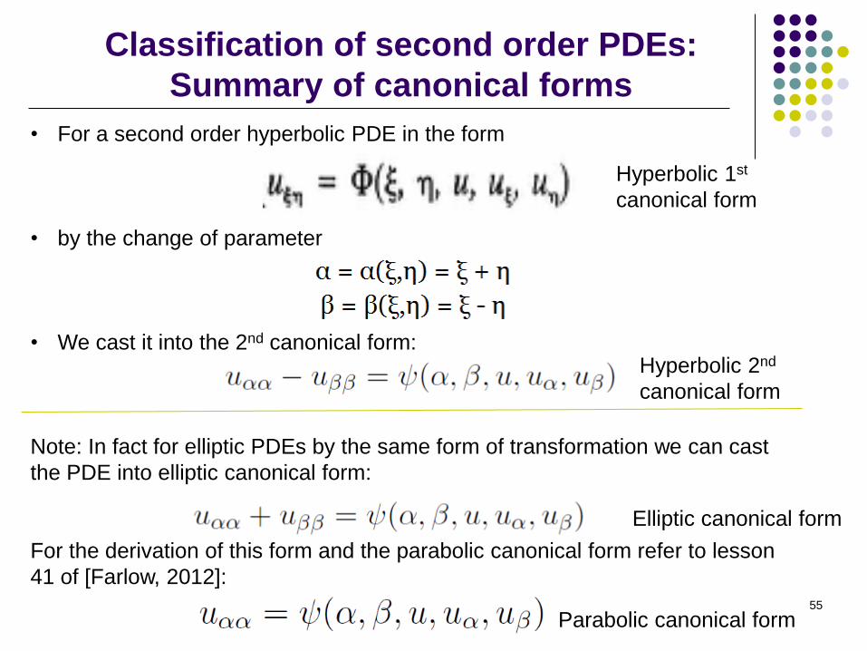
Classification of second order PDEs:
Summary of canonical forms
55
• For a second order hyperbolic PDE in the form
• by the change of parameter
• We cast it into the 2nd canonical form:
Note: In fact for elliptic PDEs by the same form of transformation we can cast
the PDE into elliptic canonical form:
For the derivation of this form and the parabolic canonical form refer to lesson
41 of [Farlow, 2012]:
Hyperbolic 2nd
canonical form
Hyperbolic 1st
canonical form
Elliptic canonical form
Parabolic canonical form
Page 36
Classification of second order PDEs:
More than 2 independent variables
56
• For a second order linear hyperbolic PDE with n independent variables:
Source: [Loret, 2008]
Note a is expressed as symmetric matrix
Page 37
Classification of second order PDEs:
More than 2 independent variables
57
Canonical form after coordinate transformation (refer to Loret chapter 3)
• Elliptic:
• Hyperbolic:
• Parabolic:
Source: [Loret, 2008]
Page 38
Classification of second order PDEs:
More than 2 independent variables
58
Comparison with 2nd order PDE with two variables:
where
has the eigenvalues derived from
Page 39
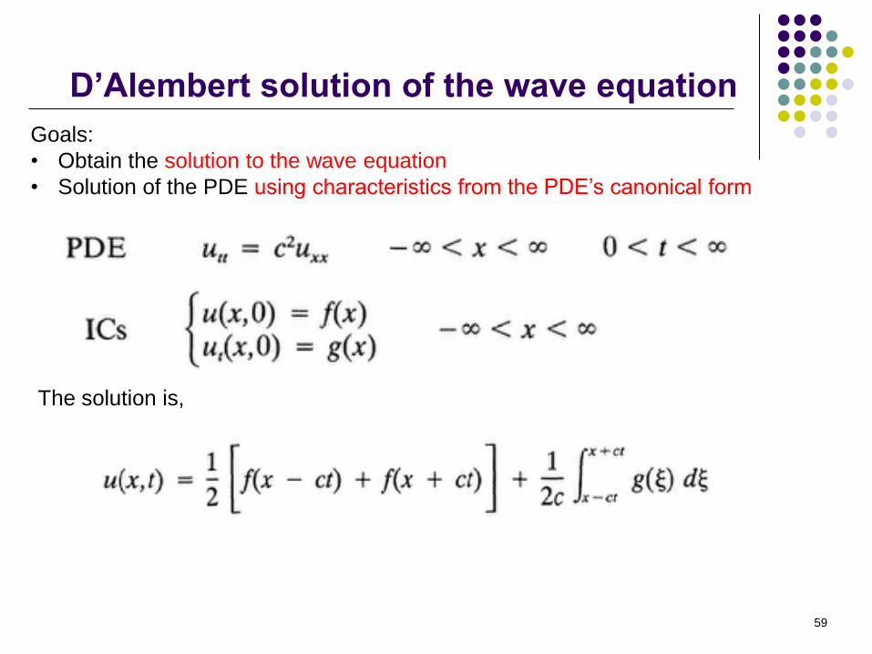
D’Alembert solution of the wave equation
59
Goals:
• Obtain the solution to the wave equation
• Solution of the PDE using characteristics from the PDE’s canonical form
The solution is,
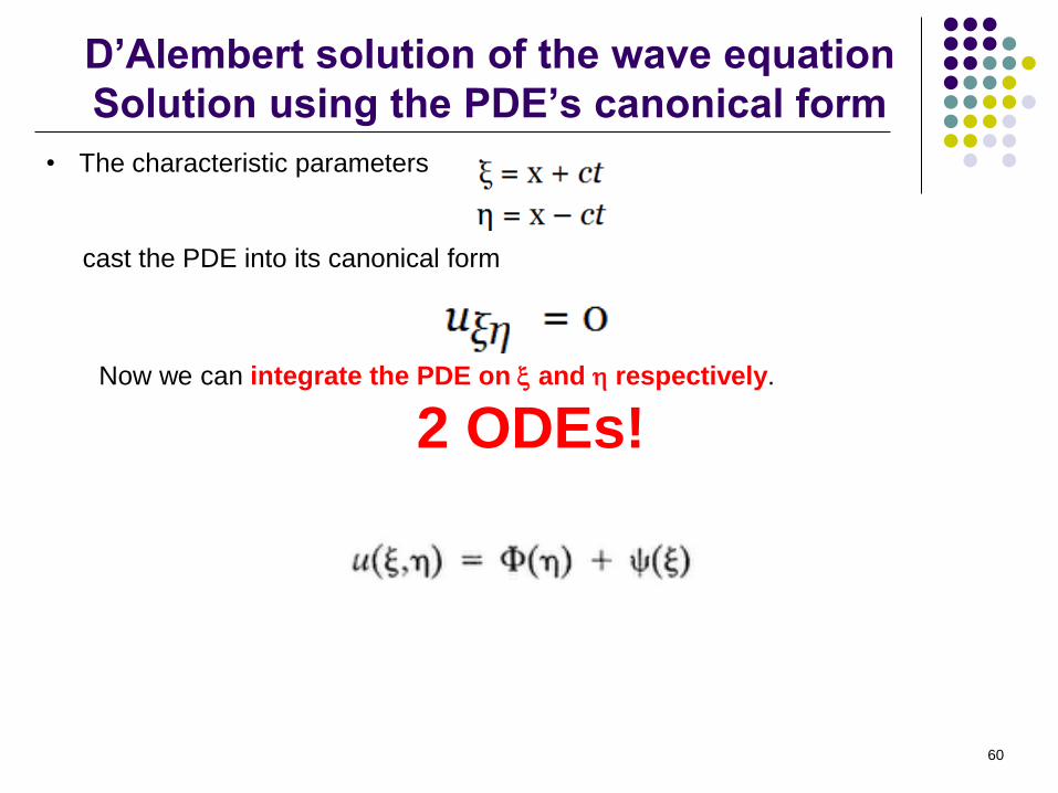
Page 40
D’Alembert solution of the wave equation
Solution using the PDE’s canonical form
60
• The characteristic parameters
cast the PDE into its canonical form
Now we can integrate the PDE on x and h respectively.
2 ODEs!
Page 41
D’Alembert solution of the wave equation
Use of initial conditions
61
• By plugging in the initial conditions we want to solve the functions f and y:
• By integrating the second equation we get
(K is set to zero because eventually in the solution of u K cancels out)
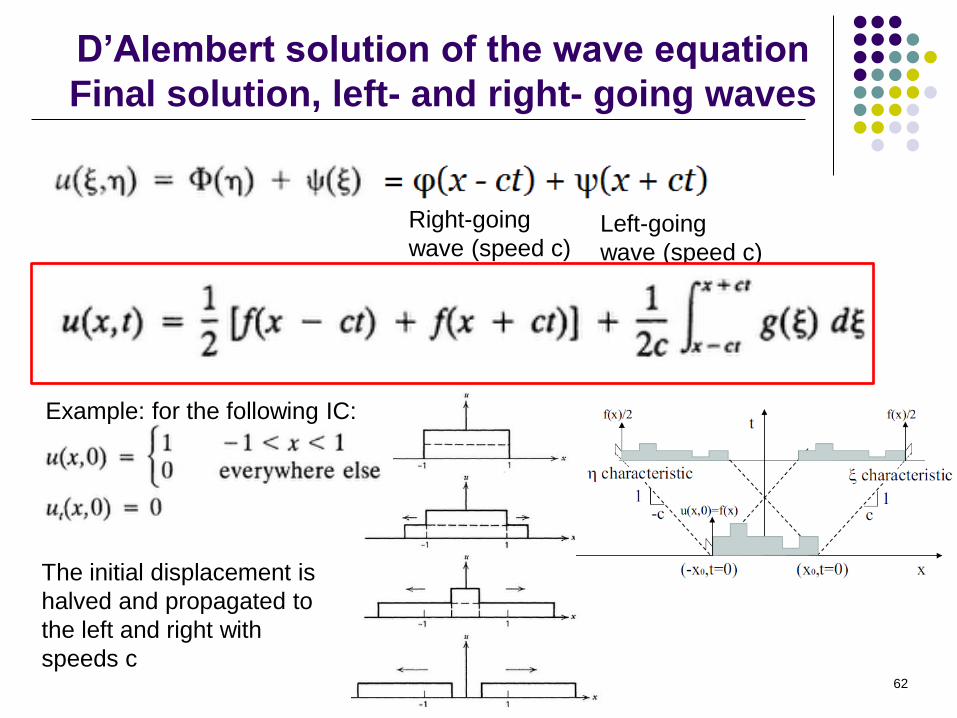
Page 42
D’Alembert solution of the wave equation
Final solution, left- and right- going waves
62
Right-going
wave (speed c) Left-going
wave (speed c)
Example: for the following IC:
The initial displacement is
halved and propagated to
the left and right with
speeds c
Page 43
Domain of influence and dependence
Finite speed of information propagation
63
Solution at x0, t0 only depends on the IC in [x0- c t0, x0+ c t0] which is called
domain of dependence
Region where the solution of (x0, t0) influences is called
domain of influence
domain of dependence
domain of
influence
Page 44
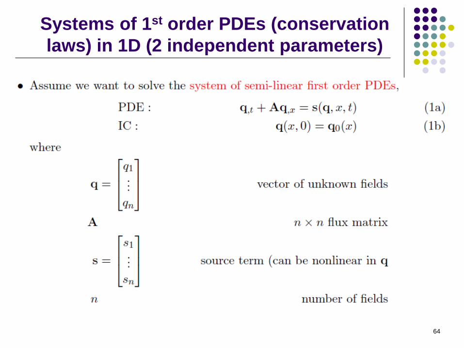
Systems of 1st order PDEs (conservation
laws) in 1D (2 independent parameters)
64
Page 45
Systems of 1st order PDEs
Characteristic values
65
Page 46
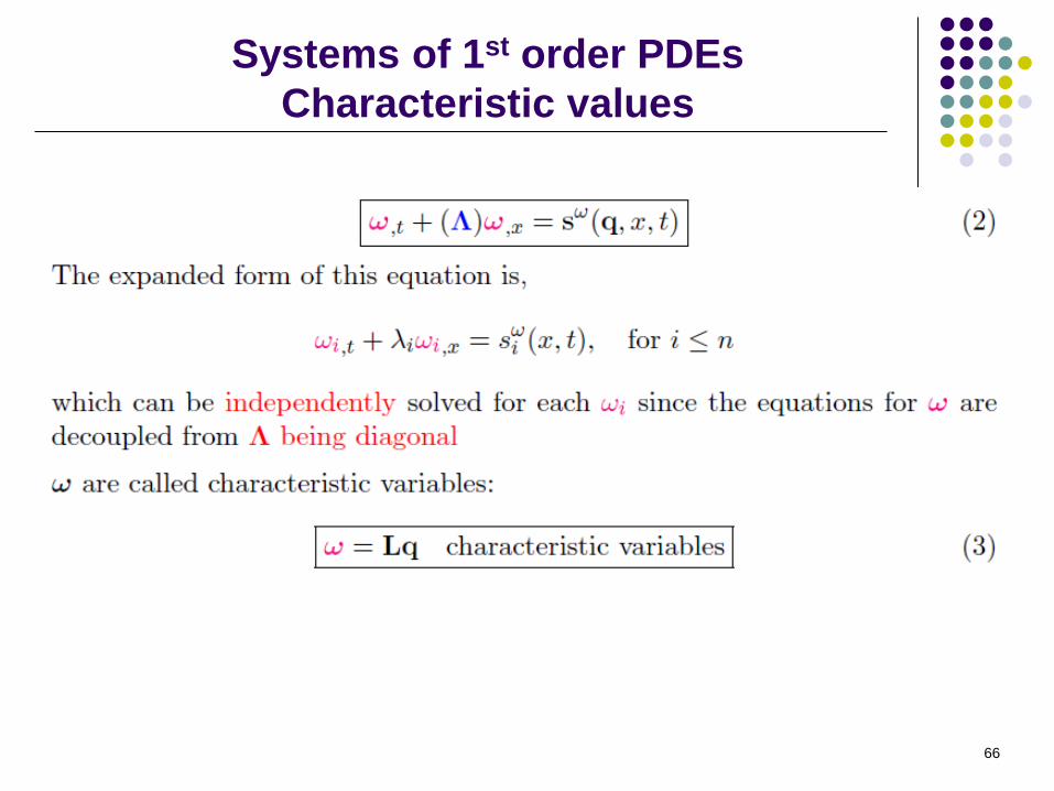
Systems of 1st order PDEs
Characteristic values
66
Page 47
Systems of 1st order PDEs
Eigenvalue problem for characteristic values
67
Page 48
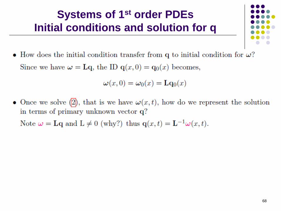
Systems of 1st order PDEs
Initial conditions and solution for q
68
Page 49
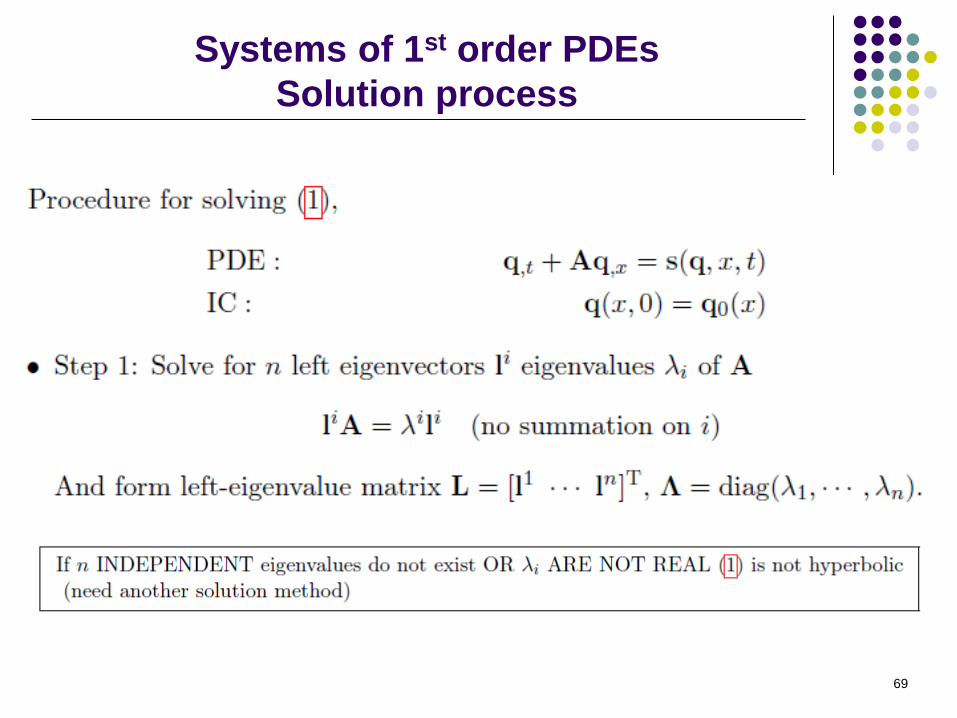
Systems of 1st order PDEs
Solution process
69
Page 50
Systems of 1st order PDEs
Solution process
70
Page 51
Systems of 1st order PDEs
Example: 1D elastodynamics problem
71
Page 52
Systems of 1st order PDEs
Example: 1D elastodynamics problem
72
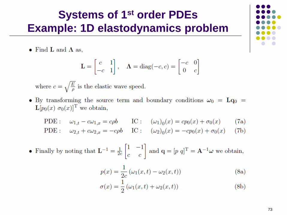
Page 53
Systems of 1st order PDEs
Example: 1D elastodynamics problem
73
Page 54
Systems of 1st order PDEs
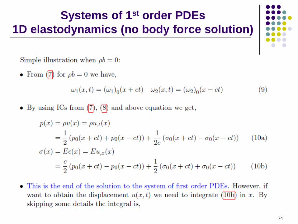
1D elastodynamics (no body force solution)
74
Page 55
Systems of 1st order PDEs
1D elastodynamics (no body force solution)
75
domain of
influence
Page 56
Systems of 1st order PDEs
Hyperbolicity condition
76
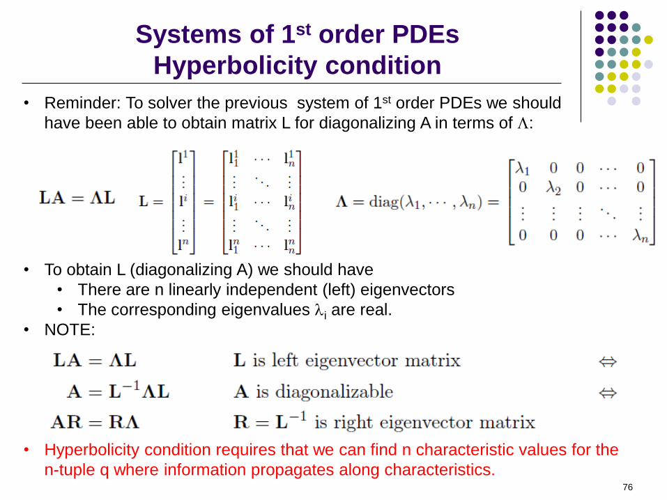
• Reminder: To solver the previous system of 1st order PDEs we should
have been able to obtain matrix L for diagonalizing A in terms of L:
• To obtain L (diagonalizing A) we should have
• There are n linearly independent (left) eigenvectors
• The corresponding eigenvalues li are real.
• NOTE:
• Hyperbolicity condition requires that we can find n characteristic values for the
n-tuple q where information propagates along characteristics.
Page 57
Geometric and algebraic multiplicity
77
Page 58
Geometric and algebraic multiplicity
78
Page 59
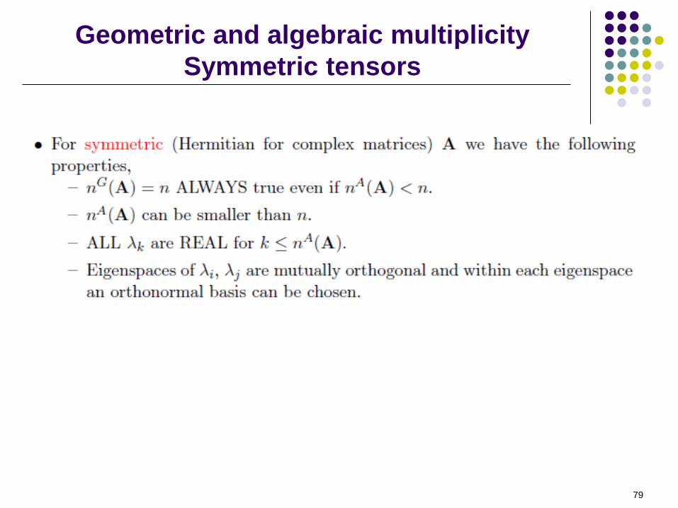
Geometric and algebraic multiplicity
Symmetric tensors
79
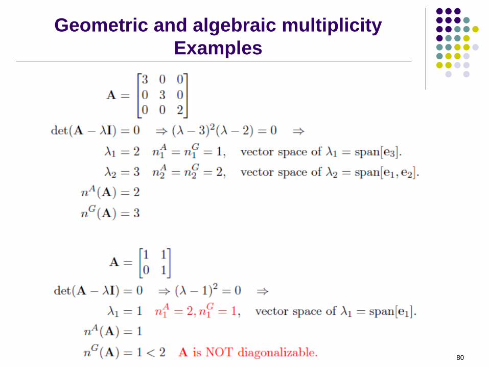
Page 60
Geometric and algebraic multiplicity
Examples
80
Page 61
Hyperbolicity of a system of 1st order PDEs
Geometric and algebraic multiplicity
81
Page 62
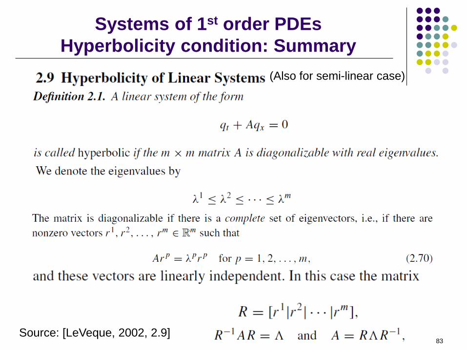
Systems of 1st order PDEs
Hyperbolicity condition: Summary
83 Source: [LeVeque, 2002, 2.9]
(Also for semi-linear case)
Page 63
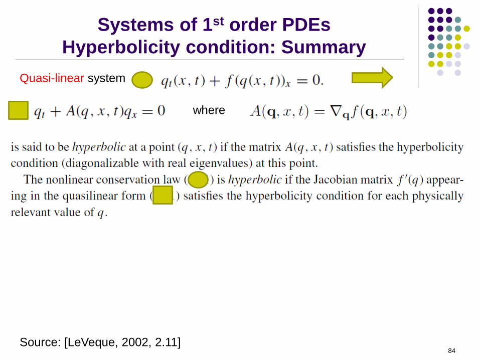
Systems of 1st order PDEs
Hyperbolicity condition: Summary
84 Source: [LeVeque, 2002, 2.11]
Quasi-linear system
where
Page 64
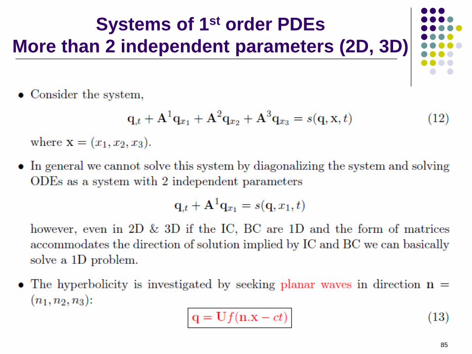
Systems of 1st order PDEs
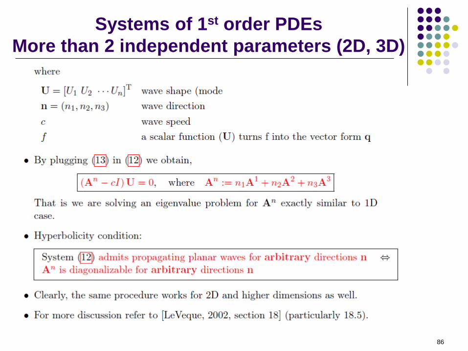
More than 2 independent parameters (2D, 3D)
85
Page 65
Systems of 1st order PDEs
More than 2 independent parameters (2D, 3D)
86
Page 66
Quasi-linear systems of 1st order PDEs
Balance laws
87
Page 67
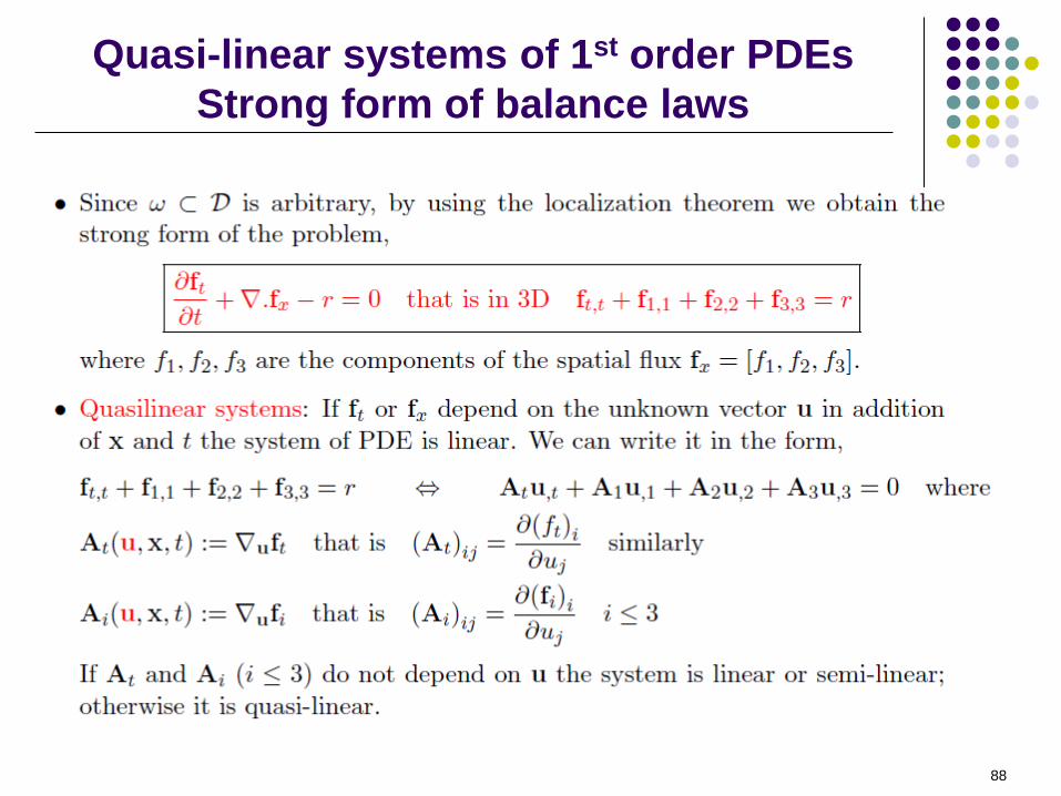
Quasi-linear systems of 1st order PDEs
Strong form of balance laws
88
Page 68
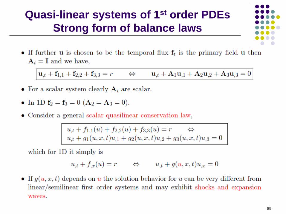
Quasi-linear systems of 1st order PDEs
Strong form of balance laws
89
Page 69
Quasi-linear 1st order PDEs
Formation of shocks & expansion wave
90
Example: Burger’s equation
Motivation: Shock and expansion waves:
Page 70
Quasi-linear 1st order PDEs
Formation of shocks & expansion wave
91
Example: Burger’s equation (continued)
Source: [Loret, 2008]
Page 71
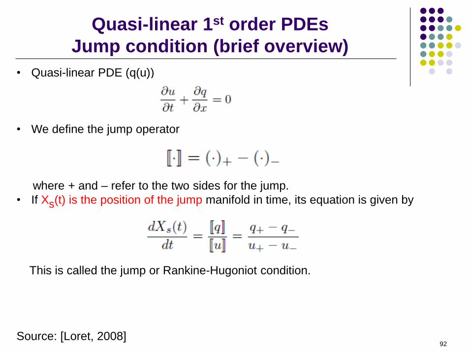
Quasi-linear 1st order PDEs
Jump condition (brief overview)
92 Source: [Loret, 2008]
• Quasi-linear PDE (q(u))
• We define the jump operator
where + and – refer to the two sides for the jump.
• If Xs(t) is the position of the jump manifold in time, its equation is given by
This is called the jump or Rankine-Hugoniot condition.
Page 72
FYI Balance laws in spacetime
(graphical view)
93
The balance law is
We can define spacetime flux by
combining spatial flux fx with
temporal flux ft (e.g. fx = -s, ft = p in
elastodynamics)
Page 73
FYI Jump condition
(graphical view)
94
By writing two balance law
expressions for W+ and W- we
obtain the jump condition
Rankine-Hugoniot
Jump conditions
• nt is the spatial component of jump manifold, by 90˚
rotation from jump to normal direction we get the – sign.
• We cannot define normal vectors in spacetime, but this
sketch provides an idea how the jump condition is derived
Page 74
Quasi-linear 1st order PDEs
Jump formation example
95
Shock formation: example Traffic flow (u is speed)
Source: [Farlow, 2012]
Initial condition
Wave has speed of 1
Wave has speed of 0
Page 75
Quasi-linear 1st order PDEs
Jump formation example
96
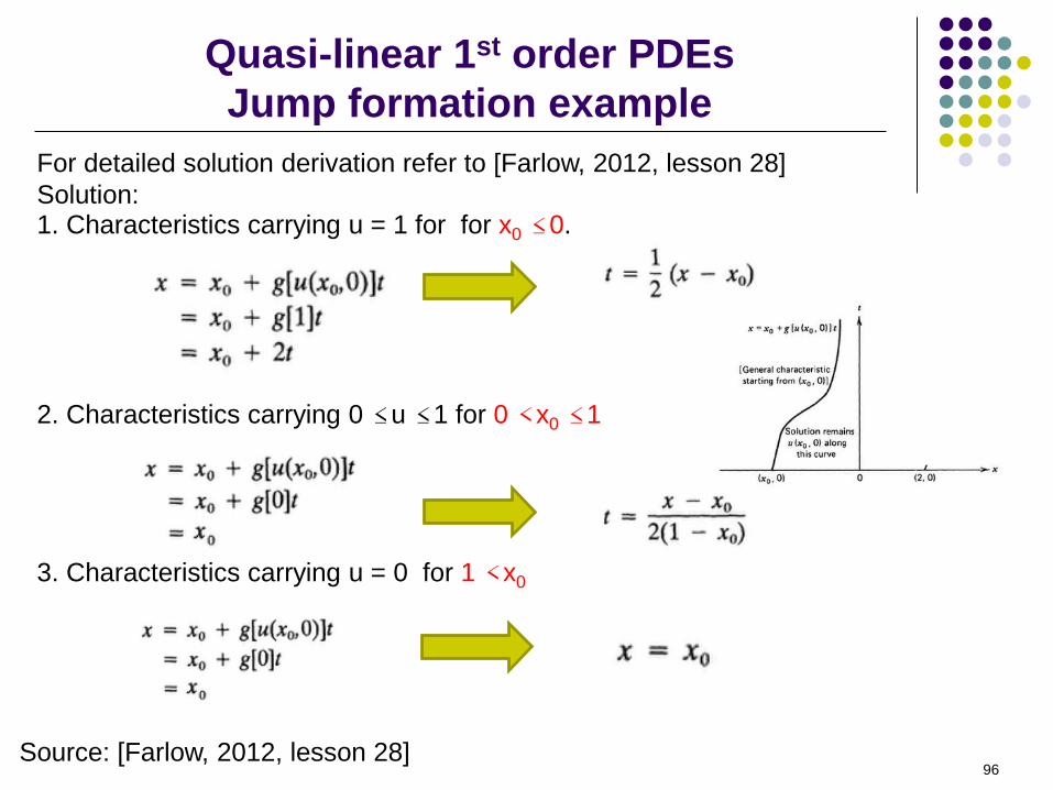
For detailed solution derivation refer to [Farlow, 2012, lesson 28]
Solution: 1. Characteristics carrying u = 1 for for x0 ≤ 0.
2. Characteristics carrying 0 ≤ u ≤ 1 for 0 < x0 ≤ 1
3. Characteristics carrying u = 0 for 1 < x0
Source: [Farlow, 2012, lesson 28]
Page 76
Quasi-linear 1st order PDEs
Jump formation example
97 Source: [Farlow, 2012, lesson 28]
Shock formed as
characteristics collide
Page 77
Quasi-linear 1st order PDEs
Jump formation example
98 Source: [Farlow, 2012, lesson 28]
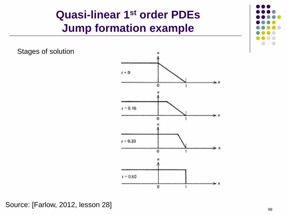
Stages of solution
Page 78
1D Acoustic equation
102
Page 79
1D Acoustic equation
103
Page 80
Riemann solution techniques
Linear conservation laws
104
Page 81
Riemann solution techniques
Linear conservation laws
105
Page 82
Riemann solution techniques
Linear conservation laws
106
Page 83
Riemann solution techniques
Linear conservation laws
107
Page 84
Riemann solution techniques
Linear conservation laws: Acoustic equation
108
Page 85
Riemann solution techniques
Linear conservation laws: Acoustic equation
109
Page 86
Riemann solution techniques
Linear conservation laws: Acoustic equation
110
Page 87
References
127
• [Bathe, 2006] Bathe, K.-J. (2006). Finite element procedures. Klaus-Jurgen Bathe.
• [Chapra and Canale, 2010] Chapra, S. C. and Canale, R. P. (2010). Numerical
methods for engineers, volume 2. McGraw-Hill. 6th edition.
• [Farlow, 2012] Farlow, S. J. (2012). Partial differential equations for scientists and
engineers. Courier Corporation.
• [Hughes, 2012] Hughes, T. J. (2012). The finite element method: linear static and
dynamic finite element analysis. Courier Corporation.
• [Levandosky, 2002] Levandosky, J. (2002). Math 220A, partial differential
equations of applied mathematics, Stanford university.
http://web.stanford.edu/class/math220a/ lecturenotes.html.
• [LeVeque, 2002] LeVeque, R. L. (2002). Finite Volume Methods for Hyperbolic
Problems. Cambridge University Press.
• [Loret, 2008] Loret, B. (2008). Notes partial differential equations PDEs, institut
national polytechnique de grenoble (inpg).
http://geo.hmg.inpg.fr/loret/enseee/maths/ loret_maths-EEE.html#TOP.
• [Strikwerda, 2004] Strikwerda, J. C. (2004). Finite difference schemes and partial
differential equations. SIAM.