Partial migration in roe deer: migratory and resident tactics are end points of a behavioural gradient determined by ecological factors
Francesca Cagnacci , Stefano Focardi , Marco Heurich , Anja Stache , A. J. Mark Hewison , Nicolas Morellet , Petter Kjellander , John D. C. Linnell , Atle Mysterud , Markus Neteler , Luca Delucchi , Federico Ossi and Ferdinando Urbano
F. Cagnacci ([email protected]), M. Neteler, L. Delucchi and F. Ossi, Biodiversity and Molecular Ecology Dept, IASMA Research and Innovation Centre, Fondazione Edmund Mach, Via Mach 1, IT-38010 San Michele all ’ Adige (TN), Italy. FO also at: UMR CNRS 5558 Dept. of Biometry and Evolutionary Biology, Univ. Claude Bernard Lyon1, Bat G. Mendel 43 Bd du 11 Novembre 1918, FR-69622 Villeurbanne Cedex, France. – S. Focardi, Istituto Superiore per la Protezione e Ricerca Ambientale, Via Ca ’ Fornacetta 9, IT-40064 Ozzano dell’Emilia, Bo, Italy. – M. Heurich and A. Stache, Dept of Research and Documentation, Bavarian Forest National Park, Freyunger Str 2, DE-94481 Grafenau, Germany. – A. J. M. Hewison and N. Morellet, Wildlife, Behaviour and Ecology Research Unit, French National Inst. for Agricultural Research (INRA Toulouse), Chemin de Borde Rouge BP 52627, FR-31326 Castanet Tolosan cedex, France. – P. Kjellander, Grims ö Wildlife Research Station, Dept. of Ecology, Swedish Univ. of Agricultural Science (SLU), SE-73091, Riddarhyttan, Sweden. – J. D. C. Linnell, Norwegian Inst. for Nature Research (NINA), PO Box 5685 Sluppen, NO-7485 Trondheim, Norway. – A. Mysterud, Centre for Ecological and Evolutionary Synthesis, Dept. Biology, Univ. of Oslo, PO Box 1066 Blindern, NO-0316 Oslo, Norway. – F. Urbano, via F.lli Pozzi 7, IT-20127 Milano, Italy.
Ungulate populations exhibiting partial migration present a unique opportunity to explore the causes of the general phe-nomenon of migration. Th e European roe deer Capreolus capreolus is particularly suited for such studies due to a wide dis-tribution range and a high level of ecological plasticity. In this study we undertook a comparative analysis of roe deer GPS location data from a representative set of European ecosystems available within the EURODEER collaborative project. We aimed at evaluating the ecological factors aff ecting migration tactic (i.e. occurrence) and pattern (i.e. timing, residence time, number of migratory trips). Migration occurrence varied between and within populations and depended on winter severity and topographic variability. Spring migrations were highly synchronous, while the timing of autumn migrations varied widely between regions, individuals and sexes. Overall, roe deer were faithful to their summer ranges, especially males. In the absence of extreme and predictable winter conditions, roe deer seemed to migrate opportunistically, in response to a tradeoff between the costs of residence in spatially separated ranges and the costs of migratory movements. Animals performed numerous trips between winter and summer ranges which depended on factors infl uencing the costs of movement such as between-range distance, slope and habitat openness. Our results support the idea that migration encom-passes a behavioural continuum, with one-trip migration and residence as its end points, while commuting and multi-trip migration with short residence times in seasonal ranges are intermediate tactics. We believe that a full understanding of the variation in tactics of temporal separation in habitat use will provide important insights on migration and the factors that infl uence its prevalence.
Th e ecology of movement has been recently recognised as a unifying paradigm in ecological research, where the identifi -cation of a movement phase or a movement mode helps clar-ify the interactions between individuals, and the surrounding ecosystem (Nathan et al. 2008). In turn, recent research has investigated how individual movement behaviour aff ects (and determines) population distribution (Turchin 1998, Mueller and Fagan 2008, Morales et al. 2010). Migrations are among the most studied movement patterns (Dingle and Drake 2007). Th e observation and analytical modelling of the individual-based, behavioural process of migration has been spurred on by the recent advances in tracking technolo-gies (Alerstam 2006, Jonsen et al. 2006, Cagnacci et al. 2010, Hebblewhite and Haydon 2010). Migrations also have obvious
consequences on population structure and dynamics (Taylor and Taylor 1977, Cheke and Tratalos 2007).
However, unifying defi nitions of migration have not been set, despite the numerous studies (Drake and Gatehouse 1995, Dingle 1996, Berthold et al. 2003, Holland et al. 2006). Dingle and Drake (2007) summarise and defi ne a variety of migration patterns which have been described in the literature. Of these, partial migration, i.e. when one frac-tion of the population is migratory, while the other remains resident, either in the breeding or non-breeding area (see also Lundberg 1988), has attracted much attention among researchers (Chapman et al. 2011). Contrasting measures of performance from migrant and non-migrant individuals off ers the opportunity to empirically evaluate the adaptive
signifi cance of migration (Lundberg 1988, Nicholson et al. 1997). In fact, in long-lived vertebrates, migration can be seen as a tactic to enhance lifetime reproductive success, which in turn is a combination of survivorship (access to food, escape from predators, avoidance of risky environmen-tal conditions) and birth rate (Fryxell and Sinclair 1988). As such, migration is presumably driven by changes in habi-tat suitability in time (e.g. seasons) and space, and can be seen as movements that allow animals to exploit temporary resources (Dingle and Drake 2007). When seasonal habitat suitability is highly variable through time, but not extreme, and some form of density dependence exists, then partial migration may evolve (Lundberg 1988, Taylor and Norris 2007). Very high variability of habitat suitability in time and space should favour migration as a ‘ direct, proximate ’ response to the deterioration of local conditions (Dingle and Drake 2007), whereas stable periodicity of habitat suitabil-ity should lead to seasonal cue-driven migration (Sabine et al. 2002). Habitat instability can therefore lead to animals migrating only in certain years or late in the season, for a short period or with several migratory trips for given individ-uals (Nelson 1995, Nicholson et al. 1997, Sabine et al. 2002, Fieberg et al. 2008). Th is behaviour is known as ‘ facultative migration ’ (Dingle and Drake 2007; ‘ conditional migration ’ has also been used to describe the same phenomenon).
When resources satisfying diff erent needs are variable ‘ in space ’ , e.g. very patchy, but relatively constant over time, we expect home ranges to comprise spatially separated resource patches, and animals to ‘ commute ’ between them, sensu Dingle and Drake (2007). Th is behaviour is a de facto example of third order habitat selection, i.e. within the home range (sensu Johnson 1980).
When resources are variable ‘ in space and time ’ (i.e. spatially separated patches constitute a suitable resource discontinuously, e.g. seasonally), commuting behaviour may become discontinuous, or opportunistic. Moreover, if travel-ling to these separated patches implies a trade-off in terms of survival (e.g. for energetic travelling costs, or exposure to predators; Nicholson et al. 1997), commuting may turn into prolonged, uninterrupted phases of residence in these patches, that if they extend over a season, can be consid-ered as ‘ seasonal ’ migration (shift in use of habitat, Dingle 1996). Under this view, the distinction between third order habitat selection, commuting behaviour and seasonal migra-tion (including partial and facultative migration) are rather unclear. Ball et al. (2001) underlined that migration is better viewed as a continuous phenomenon, where ‘ resident ’ and ‘ migrant ’ are the end points of a behavioural gradient. Din-gle and Drake (2007) encouraged investigations of migratory adaptations beyond the ‘ extremes ’ , such as, for example, fac-ultative migration, since this could reveal tradeoff s between migration and alternative adaptive strategies.
Th e European roe deer Capreolus capreolus is a small, soli-tary cervid species, with a high degree of behavioural plasticity (Jepsen and Topping 2004), and a rather peculiar combina-tion of life history traits among large herbivores of temperate areas. Indeed, this species has a relatively short generation time (Gaillard et al. 2008), is situated close to the income breeder end of the energy allocation tactic continuum (Andersen et al. 2000), shows a limited degree of sexual size dimorphism and presents two clear physiologically and behaviourally
distinct phases of the annual cycle, with birth, territoriality and rutting concentrated between May and August through-out its range (Hewison et al. 1998, Semp é r é et al. 1998). Seasonal migrations, including partial migrations, have been observed in northern environments (Wahlstr ö m and Liberg 1995, Danilkin and Hewison 1996, Mysterud 1999) and in the Alps (Ramanzin et al. 2007), where some individuals also behaved as facultative migrators. Overall, a range of tac-tics in seasonal space use have been described in these stud-ies. However, surprisingly for one of the most widely and intensively studied large mammal species in the world, little formal analysis has been devoted to this important aspect of its behaviour. In particular, insights can be obtained by con-trasting space use strategies in populations living under very diff erent climatic and ecological conditions. Th e roe deer is particularly suited for such studies due to its wide distribu-tion range in the temperate region (Andersen et al. 1998) and since detailed GPS data are available from a number of contrasting study sites across this range due to the existence of a data set repository which has recently been set up at the European scale (EURODEER; Fondazione E. Mach Trento, Italy: � www.eurodeer.org � ).
In this study, we analysed year-round GPS location data of roe deer from fi ve contrasting study areas representing dif-ferent climatic conditions, from the harsh winters of Scan-dinavia to the mild sub-Mediterranean climate of southern France. First, we quantifi ed the degree of separation of sea-sonal ranges ‘ in space and time ’ . Th en, we investigated what criteria could be used to discriminate between migrators and commuters, and therefore describe the migratory con-tinuum. Finally, we analysed the impact of climatic (snow) and topographic (slope) factors, as well as sex, on the onset and patterns of migration, starting from the following set of expected results.
In cervids, seasonal migration is often triggered by snow cover, or snow depth, or snow quality (e.g. mule deer Odocoileus hemionus : Nicholson et al. 1997; white-tailed deer Odocoileus virginianus : Sabine et al. 2002, Brinkman et al. 2005, Fieberg et al. 2008; moose Alces alces : Ball et al. 2001; roe deer: Mysterud 1999), since it infl uences both the availability of food and the cost of locomotion. However, a large variability has been observed in the responses of diff er-ent species and populations in terms of migration pattern (e.g. timing, duration, number of trips between ranges). We expected to observe migration in roe deer in areas with persistent snow cover, with partial and/or opportu-nistic migrations prevailing in less predictable climates. Moreover, we expected a direct relationship between the locomotion costs of migration and the probability of a sin-gle-trip migration, particularly given the small size of this cervid (allometric eff ect on costs of movement: White and Seymour 2005).
In several species of cervids, including roe deer, diff erent patterns of migration have been observed between the sexes, but this is highly variable (e.g. only female mule deer showed partial migration, while males were obligatory migrators: Nicholson et al. 1997; a higher proportion of migrators and longer migration distances were observed in female roe deer than in males: Mysterud 1999, but this was not observed by Ramanzin et al. 2007; no sex eff ect recorded in white tailed deer: Van Deelen et al. 1998). Th e low sexual
1792
size dimorphism in roe deer leads to the expectation of simi-lar costs and benefi ts of migration in both sexes.
Overall, we expected the marked ecological plasticity of roe deer to be mirrored by similarly marked variation in migratory behaviour, both in terms of occurrence (migration tactic) and space use (migration pattern).
Methods
Study areas and datasets
Th is study was based on a database maintained by the col-laborative EURODEER project ( � www.eurodeer.org � , accessed on 15 April 2011), i.e. a data sharing project that stores and manages roe deer data sets from across this species distribution range, involving 18 research groups from nine European countries. In particular, this repository includes more than 1 000 000 GPS locations from 354 marked indi-viduals in 13 study sites from seven countries. For this study, we selected macro-regions that represent the range of condi-tions under which most roe deer occur in Europe, and where a suitable sample was available (we excluded data from rein-troduction projects or with a small sample of individuals). Study areas, sample sizes and GPS collar models are shown in Table 1: Bavarian Forest, data from Bavarian Forest National Park (site 1: average coordinates: 49 ° 00 ’ 57 ’ ’ N, 13 ° 39 ’ 99 ’ ’ E; central European sub-mountainous forest; 650 – 1450 m a.s.l.); southern France, Coteaux de Gascogne, data from French National Inst. for Agricultural Research (INRA) (site 2: average coordinates: 43 ° 32 ’ 21 ’ ’ N, 00 ° 82 ’ 47 ’ ’ E; hilly agricultural landscape with fragmented oak woodland; alti-tude � 400 m a.s.l.); Italian eastern Alps, Trentino province, data from Fondazione Edmund Mach (site 3: average coor-dinates: 46 ° 03 ’ 27 ’ ’ N, 11 ° 02 ’ 11 ’ ’ E; Alpine mountain range from 400 to 1600 m a.s.l.); southern Scandinavia, two sites, data from Swedish Univ. of Agricultural Sciences (SLU), Norwegian Inst. for Nature Research (NINA), and Univ. of Oslo (UoO) (site 4: NINA-UoO, average coordinates: 60 ° 73 ’ 15 ’ ’ N, 08 ° 60 ’ 09 ’ ’ E; hilly area dominated by boreal forest in valleys and tundra at higher elevations, extending above the treeline; 200 – 1000 m a.s.l; site 5: SLU, average coordinates: 58 ° 10 ’ 96 ’ ’ N, 12 ° 40 ’ 78 ’ ’ E; mainly fl at boreal forest (70%) with some arable land and pastures (20%); 70 – 200 m a.s.l.). GPS data collection spanned from 2002 to 2011 and concerned 88 individuals (Table 1), with a total number of 88 760 locations. For each animal, we retained only one sampling year to avoid individual autocorrelation
(average sampling duration: 324.68 � 5.32 days). Daily fre-quency of localisation was not more than 6 (i.e. one fi x every four hours), and this was the case for 21% of locations in the data set used; otherwise, inter-fi x interval was six h for 32% of the data (i.e. four fi xes day �1 ), and eight h for 32% of the data (i.e. three fi xes day �1 ); all other fi xes were at a lon-ger interval (from 12 to 24 h), mainly due to missing fi xes. Due to this slight imbalance in sampling design of animal trajectories, only those summary parameters which can be considered independent from data density (within the above limits) were calculated.
GPS data were organised in a PostgreSQL 8.4.1 � Post-GIS 1.5.2 ( � www.postgresql.org/; http://postgis.refractions.net/ � ) spatial data base, as described in Cagnacci and Urbano (2008) and Urbano et al. (2010). GPS data were related to climatic and geographic variables from remote sens-ing sources, with a raster based automated procedure (Table 2). Snow cover was derived from the MODIS MOD10A2 eight-day composite maximum snow extent data at level V005 (data downloaded from NASA WIST, � https://wist.echo.nasa.gov � ). If snow cover was found for at least one day in the interval of eight considered, the cell was indicated as ‘ snow ’ . Using this eight-day compositing technique, the impact of clouds is minimized (Riggs et al. 2003). Th e data were processed in GRASS GIS (Neteler 2005) and snow pres-ence/absence data extracted for the EURODEER GPS fi xes.
Data analysis
Migrant and resident individuals We defi ned migration as a clear shift of an individual between non-overlapping ranges or habitats at a seasonal temporal scale (Dingle 1996), regardless of the actual Euclidian distance between those ranges. Pragmatically, we defi ned ‘ migration ’ as the process involving the shift of individuals between non-overlapping ranges ( ‘ spatial separation ’ ) and, ultimately, some stabilisation in each range ( ‘ temporal separation ’ ). We analysed the GPS locations of individuals to ascertain the occurrence of seasonal partial migration within our roe deer populations using an adaptive data-mining procedure. Our sample units were individuals or, for patterns of migration, individual tra-jectories in a given season. With a conservative approach, we considered individuals as migrants when 1) they were not fawns (not to confound migration with natal dispersal), 2) a movement between non-overlapping ranges was observed (i.e. spatial separation: individuals used non-overlapping ranges), 3) each range was continuously and solely used for a period of time (i.e. ‘ temporal separation ’ in space use), and 4) return
Table 1. Sample size, proportion of migratory individuals and migratory trajectory parameters in each study area.
Study siteGPS collar brand and
modelPeriod of reference
Migrant individuals
(m-f)Resident
individuals (m-f)
Mean no. transitions in migratory traj.
Mean Euclidean distance (m) of migratory traj.
Bavarian Forest Vectronic Aersospace Gmbh, GPS Plus 1
Southern Sweden Vectronic Aersospace Gmbh, GPS Plus 1
2007–2010 0 13 (7-5) – –
1793
winter and summer clusters, and ‘ autumn ’ , starting on 15 Sep-tember and recording transitions between summer and winter clusters. Th e starting date for spring is somewhat early to ensure that the earliest spring migrations in the most southern areas are not missed, given the very diff erent climatic conditions across Europe at this time of year.
Temporal separation: residence time, selection of migratory individuals and defi nition of migration trajectories For individuals with separated spatial ranges, we calculated the maximum residence time, i.e. the longest period of time when an animal occupied continuously (and solely) a given (win-ter or summer) range (i.e. residence time in days: sequences of type a) and b), scaling them as proportions of one year (Fig. 1). We graphically distinguished diff erent groups of ani-mals, and, in particular, we compared the position of females
movements between ranges were observed. We considered individuals as residents in all other cases.
Spatial separation: non-overlapping ranges defi nition (clustering) We applied a supervised clustering procedure (SAS 9.2, PROC CLUSTER) to identify non-overlapping ranges of individuals: we plotted the spatial distribution of fi xes in GIS software, and we counted the number of non-overlapping clusters (1 to 2). We used the method by Ward (1963) to minimize the within-cluster sum-of-squares and each fi x was assigned to a given cluster i ( i � 1,2). We then refi ned the defi nition of each cluster to remove outlying fi xes by distinguishing between locations within the cluster and excursions outside of the cluster itself using the following pro-cedure. We considered the average distance of each fi x from the nearest 10 fi xes ( d near ) and the average distance among all fi xes in a cluster i ( d all ) and its standard deviation s all . If d near � d all � s all ,we considered the fi x as part of the cluster i (assigned a cluster code of i ), otherwise, the value 0 was assigned. A fi x with code 0 there-fore represented a spatial outlier.
When more than one cluster was used by an animal, we defi ned each cluster i as a ‘ summer ’ or ‘ winter ’ cluster. We computed the average date of fi xes for each cluster i (Fisher 1993) and compared it to the 15 July (assumed to be the peak of the summer period): the summer clusters were those temporally closer to the 15 July, whereas winter clusters were all others. Migration movements were therefore studied as transitions between summer and winter clusters.
Migration movements ( ‘ shifts ’ ) and season defi nition We determined migration movements by considering the tem-poral sequence of fi xes, and their cluster code. We distinguished three types of fi x sequence: a) movements within the same clus-ter, i.e. sequences of fi xes with the same cluster code (e.g. move-ment within cluster 1: 1 →1 → 1; or movement within cluster 2: 2 → 2 → 2); b) excursions outside the perimeter of a given cluster, i.e. sequences of fi xes with a single cluster code alternating with spatial outliers (e.g. movement from cluster 1 to outliers, and back: 1 → 0 → 0→ 1); c) shifts between ranges, i.e. sequences of fi xes with diff erent cluster codes (e.g. movement between clus-ter 1 and 2: 1→ 2; or, movement between cluster 1 and 2, with two fi xes between clusters: 1 → 0 → 0 → 2); shifts are obviously directional and can be from winter to summer clusters, or vice versa. We therefore defi ned two seasons of transition: ‘ spring ’ , starting on 15 February and recording transitions between
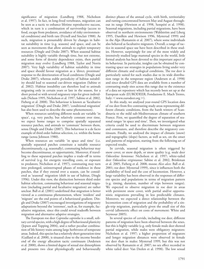
Figure 1. Maximum residence time (i.e. the maximum continuous period of residence) of migrant roe deer individuals in winter (y-axis) and summer (x-axis) ranges, expressed as a proportion of the whole year. Th e dashed line represents the limit of possible val-ues (maximum residence time in winter and summer ranges com-bined sums to one year). Blue symbols: males; red symbols: females. Squares: Bavarian Forest; diamonds: southwest France; triangles: Italian Alps; spades: Norway; circles: southern Sweden.
Table 2. Climatic and geographic variables associated with the EURODEER GPS locations and used in the analyses.
Variable Source Resolution Website
Landuse (forest cover)
EEA-Corine Landcover (CLC) 2000 (Forest: CLC 311, 312, 313, 323, 324; no forest: all others, except urban areas and inland water)
NASA-MODIS snow 3 500 m � http://modis-snow-ice.gsfc.nasa.gov/MOD10A2.html �
1 Jarvis et al. 2008 2 Hirano et al. 2003 3 Hall et al. 2002
1794
2) in each season of transition, we assessed individ-ual migratory trajectories as sequences of fi xes including migratory movements between seasonal ranges (sequences of type c). Since not all individuals presented ‘ one-hop ’ migra-tions, i.e. with only one migratory shift between ranges, but moved several times back and forth between ranges before stabilising, we defi ned the migratory trajectory as follows: in each season of transition, the sequence of fi xes starting with the fi rst shift between seasonal ranges, and fi nishing with the last seasonal shift before stabilising for a period of time ‘ equal to or greater than ’ the population average residence time as obtained from Fig. 2. Th e duration of these trajectories could therefore potentially vary from a few hours or days ( ‘ one-hop ’ migrations between ranges, e.g., movement between range 1 and 2, with one fi x between clusters: 1 → 0 → 2 → 2 → 2), to weeks or months ( ‘ multi-hop ’ migrations, e.g. movement between cluster 1 and 2, followed by return to cluster 1, followed by return to cluster 2, to then stabilise in cluster 2: 1 → 0 → 2→ 1 → 2 → 2→ 2).
Timing of migration For each migrant individual (defi ned as above), we calculated the average timing of migration from winter to summer range, and vice versa, as the average of all range shifts in that direction (sequence of type c). Timing of migration was then averaged by site (Fig. 4), sex (Fig. 3b), and over the whole dataset (Fig. 3a). Timing of migration across diff erent sampling years was necessarily represented as a circular variable, where a year is represented on the trigonometric circle with a phase of 365 and the 1 January at 0 radiant. Using this approach, a date is an angle α . Th e average date of a set of dates (as, for example, the average timing of migration) is therefore the average of a set of angles α , α 2 , … , defi ned as a vector of angle θ (the average angle) and length ρ with a value between 0 and 1. ρ is inversely proportional to the standard deviation of angles and expresses the synchrony among dates: if all dates (and angles) are the same (i.e. α � α 2 � … ) then ρ � 1; conversely, if dates (and angles) are distributed at random, then ρ � 0.
Diff erences in timing of migrations were compared across study areas and sexes using the Watson-William test (Batsche-let 1981), using 5000 bootstrap simulations (Fisher 1993).
Factors affecting migration, and the pattern of migration Migration trajectories (i.e. sequences of fi xes between the fi rst seasonal range shift and the last before stabilisation in the seasonal range, as defi ned above) were compared with similar sequences of fi xes in resident individuals (i.e. animals with only one cluster and hence no migratory movements). Trajectories of non-migrants were defi ned as the sequence of fi xes comprised between the average initial date of migration and the average fi nal date of migration for that population.
In study areas where no migrations were observed, we used the average dates calculated on the total data set.
For trajectories of both migrants and residents, we sum-marised climatic and geographic variables associated with each fi x as those in Table 2 (presence of snow cover; presence of forest cover; average slope) and calculated the Euclidean distance between the fi rst and last fi xes of the trajectory. Th e binomial variable ‘ presence of snow ’ indicates presence of snow cover at the time of any one fi x of the trajectory. Th e binomial variable ‘ presence of forest ’ was determined as fol-lows: for all trajectories in a given population, we calculated
and males on the graph by using a bivariate test computed by SAS 9.2. PROC GLM, MANOVA statement (SAS Inc. 2010); a useful discussion on the use of the Hotelling test can be found in Batschelet (1981). We then considered the frequency distribution of residence times, i.e. ‘ all ’ periods of ‘ at least ’ tw days spent continuously (and solely) by animals within a given range, and compared them across sites (Fig. 2). We used the average individual residence time as a threshold value to ascertain 1) actual temporal separation in range use (and therefore to discriminate between migrant and resident individuals) and 2) stabilisation of migratory trajectories:
1) among individuals presenting a spatial separation between ranges, only those with a maximum residence time in ‘ each ’ range of ‘ at least ’ the population average residence time were retained as migrants. Importantly, all others were designated as resident individuals. For this reason, the approach we used to ascertain the occurrence of seasonal par-tial migration was an ‘ adaptive ’ data-mining procedure based on clustering (i.e. spatial separation of ranges combined with an evaluation of actual temporal separation in range use);
Figure 2. Frequency distribution of the duration of residence (i.e. continuous periods of residence) of all migrant individuals, both in winter and summer ranges, for each study area (except Sweden, where no migrations were recorded), as well as averaged across areas. Residence periods of 1 day or less were not included.
1795
Anderson 2002). We calculated AIC values corrected for small sample size (AIC c ) for all possible models derived from the a priori full model and ranked the models according to AIC c values. From the diff erences in AIC c values ( Δ AIC c ), we cal-culated AIC c weights ( ω ) and relative evidence ratios. When Δ AIC c � 4 (relative likelihood � 0.135), we evaluated param-eter estimates by model averaging, also computing predictor weights (Burnham and Anderson 2002). To improve reliability, given the large number of models included within this cut-off , we also reassessed AIC in 999 bootstrap simulations per model, searching for the most robust model evaluations. Th e list of averaged models and corresponding parameters, including the proportion of bootstrap simulations in which they obtained the lowest AIC, are reported in Appendix 1. R2 of the average mixed models was calculated as the average sum of the rate between the variance of each model and the total variance.
Results
Spatial and temporal separation of ranges: defi nition of migratory individuals
Out of the 87 individuals from fi ve study areas considered in the analysis, we identifi ed 42 individuals with non-overlap-ping seasonal ranges. For each individual, we calculated the maximum residence time in its winter and summer range and plotted these as proportions of the whole year (Fig. 1). Note that Fig. 1 should not to be read as an X – Y chart of indepen-dent versus dependent variables, but rather as a bivariate dis-tribution plot (i.e. seasonal maximum residence times), where
the proportion of fi xes with forest cover, as well as the overall median. All values greater than the median were assigned a value of 1; all values lower than the median were assigned a value of 0.
We analysed factors aff ecting partial migration in roe deer populations by modelling the eff ect of sex, season, snow cover, presence of forest and slope on the occurrence of migration (i.e. on trajectories of both migrant and resident individu-als). In particular, we fi tted a generalized linear mixed model (GLMM) with binomial error distribution to a full model that included the additive factors listed above, including the inter-action snow slope season, as fi xed factors, and study area as a random factor (Table 3). For migration trajectories only, we analysed factors aff ecting the pattern of migration by mod-elling the eff ect of sex, season, snow cover, presence of forest, slope and Euclidean distance on the occurrence of a single trip ( ‘ one-hop ’ ) migration. In particular, we fi tted a generalized linear mixed model (GLMM) with binomial error distribu-tion to a full model that included the additive factors listed above, including the interaction snow slope, as fi xed factors and study area as a random factor. By co-plotting the response variables and the groups of predictor variables we observed that the interaction between snow, slope and season was espe-cially informative. Individual identity was not included as a random factor since only one year ’ s monitoring per individual was retained in order to analyse a balanced dataset. All linear analyses were run in R (ver. 2.9.1: R Development Core Team 2009, lme4 R package: Bates and Maechler 2009).
Response variables were modelled for dependence on pre-dictor variables using the model selection procedure based on the Akaike information criterion (AIC) (Burnham and
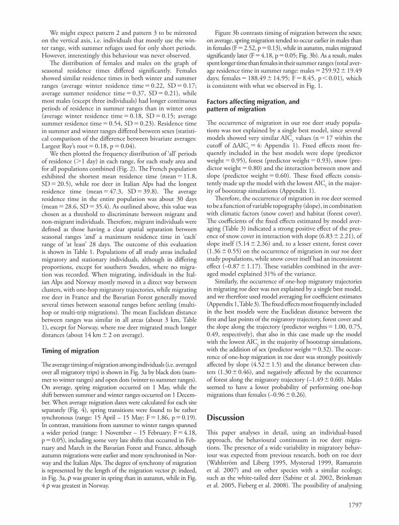
Figure 3. Timing of migrations in roe deer pooled across sample areas in Europe (panel a, grey and black), and pooled across sample areas in Europe, but classifi ed by sex (panel b, red and blue). Goniometric circles represent the year (months to be read anti-clock wise, from January to December). Panel a: dots indicate the individual average time of migration from winter to summer ranges (open dots) and from summer to winter ranges (fi lled dots). Arrows point to the average migration date across the population, in spring-summer (open headed arrow) and in autumn-winter (closed headed arrow). Th e length of the arrow ( ρ , from 0 to 1) is inversely proportional to the standard deviation of migration dates among individuals, therefore indicating the degree of migration synchrony among individuals (high ρ , long arrow � high degree of synchrony). Triangles within the goniometric circle represent the circular histogram of the frequency distribution of excursion movements (i.e. those movements that did not result in the animal reaching a second range) originating from summer ranges (grey bars) and from winter ranges (black bars). Values are expressed as a percentage of all excursions throughout the year. Panel b: symbols as in panel a except: blue dots and arrows: males; red dots and arrows: females.
1796
ing from values of 1.0 to 0.0 along the horizontal axis, these individuals spent a decreasing length of time as residents in the summer range.
In particular, individuals within the small triangle at the extreme right of the graph, were resident in the sum-mer range for most of the year, before moving to the win-ter area for a short residence period. Th ese animals appear to have a main range and a secondary one, used as a ‘ win-ter refuge ’ .
Pattern 3 When the imbalance between summer and winter range use becomes extreme, it is always the summer range that is pre-dominantly used, with only very short (e.g. two days) inter-ruptions in a secondary range. In the graph, these individuals are represented by the points which virtually lie on the hori-zontal axis. Th ese animals appear to have non-overlapping ranges that are ‘ selected ’ diff erently.
Pattern 4 Finally, individuals within the extreme left square area of the graph have similar length, but very short, continuous residence times in both non-overlapping ranges. Th ese ani-mals appear to use spatially separated ranges in a similar way, without any clear temporal separation and therefore appear to be ‘ commuting ’ between ranges.
Pattern 3 and pattern 4 look like ‘ dead ends ’ on the migratory continuum, where only one of the two conditions for migration is respected: i.e. ‘ spatial, but not temporal ’ , separation in range use.
both X and Y are dependent variables. Th is representation is useful for clarifying the pattern of contrasting use of non-over-lapping ranges by diff erent individuals:
Th e dashed line in the graph represents the limit of pos-sible values, since the maximum residence time in winter and summer ranges combined cannot exceed one year. In this case (i.e. sum � 1), the animal would stay continuously in one range, then move very fast ( � 1 day) to the second one and immediately ‘ stabilise ’ there. Th is was actually the case for one individual in the Bavarian Forest.
All points below the dashed line do not sum to 1.0, mean-ing that the continuous periods of residence in one range were interrupted by several shifts to the other range (or by a migratory shift lasting several days).
Moreover, we identifi ed the following ‘ patterns ’ of use of non-overlapping ranges:
Pattern 1 All individuals within the central triangle of the graph had a long maximum residence time in both winter and summer ranges (i.e. between one and three quarters of the year: values � 0.25 – 0.75). Th ey all showed a similar use of non-overlapping ranges: they were stable in one range for a long continuous period, then shifted a few times between ranges, before fi nally stabilis-ing again in the second range. Th ese animals could therefore be considered as performing a ‘ classical ’ migration, showing a clear spatial ‘ and ’ temporal separation in range use.
Pattern 2 All individuals below the central triangle stayed continuously in the winter range for less than a quarter of the year. Mov-
Table 3. Parameter estimates using model averaging to describe the seasonal migration of C. capreolus in Europe. Estimates were obtained from generalized linear mixed models with a binomial distribution of errors. Model selection was based on the Akaike information criterion corrected for small sample sizes (AICc). The full a priori model is given, with parameters estimated by model averaging, based on a cut-off of relative likelihood of model i versus the ‘best’ model of about 0.15 (ΔAICc≈4, evidence ratios ≈7). Models describe (a) the occurrence of migration, (b) the occurrence of direct (i.e. one-hop) migration trajectories between seasonal ranges (migrant individuals only).
apresence of snow cover along the migratory trajectorybmean slope along the migratory trajectory, arcsine transformedcseasons of transitions, starting on 15 February (spring-summer) and 15 September (autumn–winter)dpresence of forest cover along the migratory trajectory; all values above the median of all trajectories were set to 1; 0 otherwiseeEuclidean distance between fi rst and last point of the migratory trajectory, log transformedfsample size
1797
Figure 3b contrasts timing of migration between the sexes; on average, spring migration tended to occur earlier in males than in females (F � 2.52, p � 0.13), while in autumn, males migrated signifi cantly later (F � 4.18, p � 0.05; Fig. 3b). As a result, males spent longer time than females in their summer ranges (total aver-age residence time in summer range: males � 259.92 � 19.49 days; females � 188.49 � 14.95; F � 8.45, p � 0.01), which is consistent with what we observed in Fig. 1.
Factors affecting migration, and pattern of migration
Th e occurrence of migration in our roe deer study popula-tions was not explained by a single best model, since several models showed very similar AIC c values (n � 17 within the cutoff of Δ AIC c � 4: Appendix 1). Fixed eff ects most fre-quently included in the best models were slope (predictor weight � 0.95), forest (predictor weight � 0.93), snow (pre-dictor weight � 0.80) and the interaction between snow and slope (predictor weight � 0.60). Th ese fi xed eff ects consis-tently made up the model with the lowest AIC c in the major-ity of bootstrap simulations (Appendix 1).
Th erefore, the occurrence of migration in roe deer seemed to be a function of variable topography (slope), in combination with climatic factors (snow cover) and habitat (forest cover). Th e coeffi cients of the fi xed eff ects estimated by model aver-aging (Table 3) indicated a strong positive eff ect of the pres-ence of snow cover in interaction with slope (6.83 � 2.21), of slope itself (5.14 � 2.36) and, to a lesser extent, forest cover (1.36 � 0.55) on the occurrence of migration in our roe deer study populations, while snow cover itself had an inconsistent eff ect ( – 0.87 � 1.17). Th ese variables combined in the aver-aged model explained 31% of the variance.
Similarly, the occurrence of one-hop migratory trajectories in migrating roe deer was not explained by a single best model, and we therefore used model averaging for coeffi cient estimates (Appendix 1, Table 3). Th e fi xed eff ects most frequently included in the best models were the Euclidean distance between the fi rst and last points of the migratory trajectory, forest cover and the slope along the trajectory (predictor weights � 1.00, 0.75, 0.49, respectively), that also in this case made up the model with the lowest AIC c in the majority of bootstrap simulations, with the addition of sex (predictor weight � 0.32). Th e occur-rence of one-hop migration in roe deer was strongly positively aff ected by slope (4.52 � 1.5) and the distance between clus-ters (1.30 � 0.46), and negatively aff ected by the occurrence of forest along the migratory trajectory ( – 1.49 � 0.60 ) . Males seemed to have a lower probability of performing one-hop migrations than females ( – 0.96 � 0.26 ) .
Discussion
Th is paper analyses in detail, using an individual-based approach, the behavioural continuum in roe deer migra-tions. Th e presence of a wide variability in migratory behav-iour was expected from previous research, both on roe deer (Wahlstr ö m and Liberg 1995, Mysterud 1999, Ramanzin et al. 2007) and on other species with a similar ecology, such as the white-tailed deer (Sabine et al. 2002, Brinkman et al. 2005, Fieberg et al. 2008). Th e possibility of analysing
We might expect pattern 2 and pattern 3 to be mirrored on the vertical axis, i.e. individuals that mostly use the win-ter range, with summer refuges used for only short periods. However, interestingly this behaviour was never observed.
Th e distribution of females and males on the graph of seasonal residence times diff ered signifi cantly. Females showed similar residence times in both winter and summer ranges (average winter residence time � 0.22, SD � 0.17; average summer residence time � 0.37, SD � 0.21), while most males (except three individuals) had longer continuous periods of residence in summer ranges than in winter ones (average winter residence time � 0.18, SD � 0.15; average summer residence time � 0.54, SD � 0.23). Residence time in summer and winter ranges diff ered between sexes (statisti-cal comparison of the diff erence between bivariate averages: Largest Roy ’ s root � 0.18, p � 0.04).
We then plotted the frequency distribution of ‘ all ’ periods of residence ( � 1 day) in each range, for each study area and for all populations combined (Fig. 2). Th e French population exhibited the shortest mean residence time (mean � 11.8, SD � 20.5), while roe deer in Italian Alps had the longest residence time (mean � 47.3, SD � 39.8). Th e average residence time in the entire population was about 30 days (mean � 28.6, SD � 35.4). As outlined above, this value was chosen as a threshold to discriminate between migrant and non-migrant individuals. Th erefore, migrant individuals were defi ned as those having a clear spatial separation between seasonal ranges ‘ and ’ a maximum residence time in ‘ each ’ range of ‘ at least ’ 28 days. Th e outcome of this evaluation is shown in Table 1. Populations of all study areas included migratory and stationary individuals, although in diff ering proportions, except for southern Sweden, where no migra-tion was recorded. When migrating, individuals in the Ital-ian Alps and Norway mostly moved in a direct way between clusters, with one-hop migratory trajectories, while migrating roe deer in France and the Bavarian Forest generally moved several times between seasonal ranges before settling (multi-hop or multi-trip migrations). Th e mean Euclidean distance between ranges was similar in all areas (about 3 km, Table 1), except for Norway, where roe deer migrated much longer distances (about 14 km � 2 on average).
Timing of migration
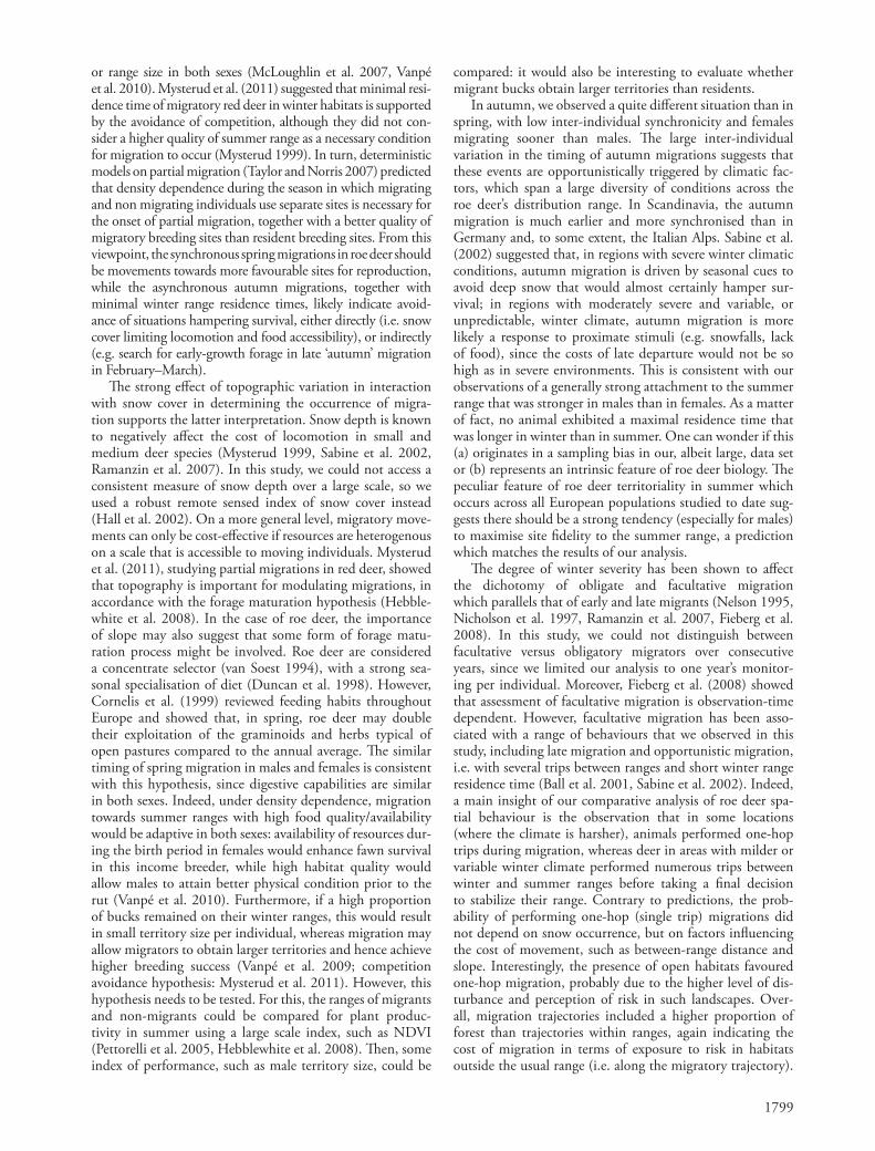
Th e average timing of migration among individuals (i.e. averaged over all migratory trips) is shown in Fig. 3a by black dots (sum-mer to winter ranges) and open dots (winter to summer ranges). On average, spring migration occurred on 1 May, while the shift between summer and winter ranges occurred on 1 Decem-ber. When average migration dates were calculated for each site separately (Fig. 4), spring transitions were found to be rather synchronous (range: 15 April – 15 May; F � 1.86, p � 0.19). In contrast, transitions from summer to winter ranges spanned a wider period (range: 1 November – 15 February; F � 4.18, p � 0.05), including some very late shifts that occurred in Feb-ruary and March in the Bavarian Forest and France, although autumn migrations were earlier and more synchronised in Nor-way and the Italian Alps. Th e degree of synchrony of migration is represented by the length of the migration vector ρ ; indeed, in Fig. 3a, ρ was greater in spring than in autumn, while in Fig. 4 ρ was greatest in Norway.
1798
summer range (i.e. ‘ autumn ’ migration in February – March in some study areas; Ramanzin et al. 2007, Fieberg et al. 2008); as a consequence, residence in the winter range was often fragmented in time (i.e. interrupted by several ‘ return ’ trips to the summer range) or limited to a very short period. Several of these patterns have been observed in deer in areas with mild or unpredictable winter conditions, and are com-mon in facultative migrators (Nelson 1995, Sabine et al. 2002, Brinkman et al. 2005).
Fourth, the occurrence of migration did not diff er between sexes, however, we observed a clear diff erence between the sexes in terms of the attachment to their summer range: males migrated later than females in autumn and resided longer in the summer range than females. Th is is not always the case in other deer species (e.g. mule deer, Nicholson et al. 1997).
Th e European roe deer takes full advantage of the evident seasonality in the European temperate region, concentrat-ing its reproductive physiology and behaviour in the sum-mer months (Semp é r é et al. 1998, Liberg et al. 1998); this, together with the observation that it is an income breeder (Andersen et al. 2000), strongly suggests the importance of the summer range for maximising reproductive success in this species, with a positive eff ect of habitat quality and/
a large scale data set that covers a considerable part of the roe deer ’ s distribution range, available here through the col-laborative EURODEER project, allowed us to identify some unexpected features in the pattern of roe deer space use and migratory behaviour in general. First, the occurrence of migra-tion was not aff ected by the simple presence of snow as a ‘ sole factor ’ , but mainly by the interaction between topographic variation (expressed as average slope) and snow cover. Con-trary to expectations (Wahlstr ö m and Liberg 1995, Mysterud 1999), migrations were indeed not observed in areas with considerable snow cover, but which are topographically fl at (southern Sweden), while some degree of migratory behav-iour was observed in areas with virtually no snow cover, but which are rather hilly (southern France).
Second, when migration was observed, roe deer individu-als concentrated their range use within a wintering area for at least part of the winter, before migrating to a separate sum-mer range, with a high degree of synchrony of this move-ment among study areas. Indeed, summer ranges were used for an equal duration or, in most cases, for longer than win-ter ranges across all study sites.
Th ird, autumn migration was highly asynchronous across study sites, and included a few very late departures from the
Figure 4. Timing of migrations in roe deer in the four study areas where migration was observed: the Bavarian Forest (1), southwest France (2), the Italian Alps (3) and Norway (4). Symbols as in Figure 3a.
1799
compared: it would also be interesting to evaluate whether migrant bucks obtain larger territories than residents.
In autumn, we observed a quite diff erent situation than in spring, with low inter-individual synchronicity and females migrating sooner than males. Th e large inter-individual variation in the timing of autumn migrations suggests that these events are opportunistically triggered by climatic fac-tors, which span a large diversity of conditions across the roe deer ’ s distribution range. In Scandinavia, the autumn migration is much earlier and more synchronised than in Germany and, to some extent, the Italian Alps. Sabine et al. (2002) suggested that, in regions with severe winter climatic conditions, autumn migration is driven by seasonal cues to avoid deep snow that would almost certainly hamper sur-vival; in regions with moderately severe and variable, or unpredictable, winter climate, autumn migration is more likely a response to proximate stimuli (e.g. snowfalls, lack of food), since the costs of late departure would not be so high as in severe environments. Th is is consistent with our observations of a generally strong attachment to the summer range that was stronger in males than in females. As a matter of fact, no animal exhibited a maximal residence time that was longer in winter than in summer. One can wonder if this (a) originates in a sampling bias in our, albeit large, data set or (b) represents an intrinsic feature of roe deer biology. Th e peculiar feature of roe deer territoriality in summer which occurs across all European populations studied to date sug-gests there should be a strong tendency (especially for males) to maximise site fi delity to the summer range, a prediction which matches the results of our analysis.
Th e degree of winter severity has been shown to aff ect the dichotomy of obligate and facultative migration which parallels that of early and late migrants (Nelson 1995, Nicholson et al. 1997, Ramanzin et al. 2007, Fieberg et al. 2008). In this study, we could not distinguish between facultative versus obligatory migrators over consecutive years, since we limited our analysis to one year ’ s monitor-ing per individual. Moreover, Fieberg et al. (2008) showed that assessment of facultative migration is observation-time dependent. However, facultative migration has been asso-ciated with a range of behaviours that we observed in this study, including late migration and opportunistic migration, i.e. with several trips between ranges and short winter range residence time (Ball et al. 2001, Sabine et al. 2002). Indeed, a main insight of our comparative analysis of roe deer spa-tial behaviour is the observation that in some locations (where the climate is harsher), animals performed one-hop trips during migration, whereas deer in areas with milder or variable winter climate performed numerous trips between winter and summer ranges before taking a fi nal decision to stabilize their range. Contrary to predictions, the prob-ability of performing one-hop (single trip) migrations did not depend on snow occurrence, but on factors infl uencing the cost of movement, such as between-range distance and slope. Interestingly, the presence of open habitats favoured one-hop migration, probably due to the higher level of dis-turbance and perception of risk in such landscapes. Over-all, migration trajectories included a higher proportion of forest than trajectories within ranges, again indicating the cost of migration in terms of exposure to risk in habitats outside the usual range (i.e. along the migratory trajectory).
or range size in both sexes (McLoughlin et al. 2007, Vanp é et al. 2010). Mysterud et al. (2011) suggested that minimal resi-dence time of migratory red deer in winter habitats is supported by the avoidance of competition, although they did not con-sider a higher quality of summer range as a necessary condition for migration to occur (Mysterud 1999). In turn, deterministic models on partial migration (Taylor and Norris 2007) predicted that density dependence during the season in which migrating and non migrating individuals use separate sites is necessary for the onset of partial migration, together with a better quality of migratory breeding sites than resident breeding sites. From this viewpoint, the synchronous spring migrations in roe deer should be movements towards more favourable sites for reproduction, while the asynchronous autumn migrations, together with minimal winter range residence times, likely indicate avoid-ance of situations hampering survival, either directly (i.e. snow cover limiting locomotion and food accessibility), or indirectly (e.g. search for early-growth forage in late ‘ autumn ’ migration in February – March).
Th e strong eff ect of topographic variation in interaction with snow cover in determining the occurrence of migra-tion supports the latter interpretation. Snow depth is known to negatively aff ect the cost of locomotion in small and medium deer species (Mysterud 1999, Sabine et al. 2002, Ramanzin et al. 2007). In this study, we could not access a consistent measure of snow depth over a large scale, so we used a robust remote sensed index of snow cover instead (Hall et al. 2002). On a more general level, migratory move-ments can only be cost-eff ective if resources are heterogenous on a scale that is accessible to moving individuals. Mysterud et al. (2011), studying partial migrations in red deer, showed that topography is important for modulating migrations, in accordance with the forage maturation hypothesis (Hebble-white et al. 2008). In the case of roe deer, the importance of slope may also suggest that some form of forage matu-ration process might be involved. Roe deer are considered a concentrate selector (van Soest 1994), with a strong sea-sonal specialisation of diet (Duncan et al. 1998). However, Cornelis et al. (1999) reviewed feeding habits throughout Europe and showed that, in spring, roe deer may double their exploitation of the graminoids and herbs typical of open pastures compared to the annual average. Th e similar timing of spring migration in males and females is consistent with this hypothesis, since digestive capabilities are similar in both sexes. Indeed, under density dependence, migration towards summer ranges with high food quality/availability would be adaptive in both sexes: availability of resources dur-ing the birth period in females would enhance fawn survival in this income breeder, while high habitat quality would allow males to attain better physical condition prior to the rut (Vanp é et al. 2010). Furthermore, if a high proportion of bucks remained on their winter ranges, this would result in small territory size per individual, whereas migration may allow migrators to obtain larger territories and hence achieve higher breeding success (Vanp é et al. 2009; competition avoidance hypothesis: Mysterud et al. 2011). However, this hypothesis needs to be tested. For this, the ranges of migrants and non-migrants could be compared for plant produc-tivity in summer using a large scale index, such as NDVI (Pettorelli et al. 2005, Hebblewhite et al. 2008). Th en, some index of performance, such as male territory size, could be
1800
and habitat fragmentation, or genetic and physiological pro-fi les (Dingle and Drake 2007, Bolger et al. 2008). We believe that a full understanding of the behavioural gradient in space use leading to diff erent kinds and degrees of migration, and the factors aff ecting it (Dingle and Drake 2007), should be one of the main fi elds of research of spatial ecology.
Acknowledgements – Th is paper was conceived and written within the collaborative EURODEER project (paper no. 001 of the EURODEER series; < www.eurodeer.org > ). Th e co-authors are grateful to all mem-bers for their support for the initiative. Th e EURODEER spatial data-base is hosted by Fondazione Edmund Mach. Th e GPS data collection of the Fondazione Edmund Mach was supported by the Autonomous Province of Trento under grant no. 3479 to FC (BECOCERWI – Behavioural Ecology of Cervids in Relation to Wildlife Infections). FC thanks the Wildlife and Forest Service of the Autonomous Prov-ince of Trento and the Hunting Association of Trento Province (ACT) for support and help during captures. Financial support for GPS data collection in the Bavarian Forest was provided by the EU-programme INTERREG IV (EFRE Ziel 3) and the Bavarian Forest National Park Administration. Th e Swedish study was supported by grants from the private foundation of ‘ Marie Claire Cronstedts Minne ’ , Th e Swedish Environmental Protection Agency and Th e Swedish Association for Hunting and Wildlife Management. MH and NM would like to thank the local hunting associations, the F é d é ration D é partementale des Chasseurs de la Haute Garonne, as well as numerous co-workers and volunteers for their assistance and, in particular, B. Cargnelutti, J.M. Angibault, B. Lourtet and J. Merlet. Th e Norwegian data collec-tion was funded by the Directorate for Nature Management and the county administration of Buskerud county.
References
Alerstam, T. 2006. Confl icting evidence about long-distance ani-mal navigation. – Science 313: 791 – 794.
Andersen, R. et al. 1998. Th e European roe deer: the biology of success. – Scandinavian Univ. Press.
Andersen, R. et al. 2000. Factors aff ecting maternal care in an income breeder, the European roe deer. – J. Anim. Ecol. 69: 672 – 682.
Ball, P. et al. 2001. Partial migration by large ungulates: character-istics of seasonal moose Alces alces ranges in northern Sweden. – Wildlife Biol. 7: 39 – 47.
Bates, D. and Maechler, M. 2009 lme4 package for R. – � http://lme4.r-forge.r-project.org/ �
Batschelet, E. 1981. Circular statistics in biology. – Academic Press. Berthold, P. et al. 2003. Avian migration. – Springer. Bolger, D. T. et al. 2008. Th e need for integrative approaches to under-
stand and conserve migratory ungulates. – Ecol. Lett. 11: 63 – 77. Brinkman, T. J. et al. 2005. Movement of female white-tailed deer:
eff ects of climate and intensive row-crop agriculture. – J. Wild-life Manage. 69: 1099 – 1111.
Burnham, K. P. and Anderson, D.R. 2002. Model selection and multimodel inference: a practical information-theoretic approach, 2nd ed. – Springer.
Cagnacci, F. and Urbano, F. 2008. Managing widlife: a spatial information system for GPS collar data. – Environ. Modell. Softw. 23: 957 – 959.
Cagnacci, F. et al. 2010. Animal ecology meets GPS-based radio-telemetry: a perfect storm of opportunities and challenges. – Phil. Trans. R. Soc. B 365: 2157 – 2162.
Chapman, B. B. et al. 2011. Th e ecology and evolution of partial migration. – Oikos 120: 1764–1775.
Cheke, R. A. and Tratalos, J. A. 2007. Migration, patchiness, and population processes illustrated by two migrant pests. – Bio-science 57: 145 – 154.
It seems likely that frequent shifts between ranges are explor-atory movements, necessary for evaluating the suitability of the new range and the appropriate timing for settling. We presume that such a strategy would be favoured when the costs of range shifts are low, while when such costs are large a one-hop trip should be more eff ective.
Th e pattern of migration in southern France appears to be rather diff erent from the other study areas, with a less clear separation between spring and autumn migrations, short resi-dence times in alternative ranges and multi-hop trajectories. Th is higher variability strongly suggests that, in this envi-ronment, roe deer behave as commuters (Dingle and Drake 2007), moving between separate ranges throughout the year, with very limited continuous residence time. Th is tactic of seasonal space use may ‘ collapse ’ into third order habitat selec-tion of multi-patch home ranges in the most extreme cases.
Th e results of our large scale analysis overall suggest that, in roe deer, migratory behaviour is quite opportunistic, and partial migration appears to be the rule rather than the excep-tion in this species. Similar conclusions were derived from a long-term study on white-tailed deer (Fieberg et al. 2008). Th e high ecological plasticity and wide distribution range of these deer species may allow us to empirically investigate the fundamental nature of migration as a tactic of space use, where the costs of residence in spatially separated ranges are traded-off against the costs of migratory movement. As such, ‘ migratory ’ behaviour is the end point of a behavioural gradient that includes ‘ residence ’ at the other extreme, with ‘ commuting ’ and ‘ facultative ’ or opportunistic (multi-trip) migration as intermediate tactics. Interestingly, facultative migration between two separate ranges challenges the dis-tinction between second and third order habitat selection (Johnson 1980), or at least requires the extension of this defi nition to cover an extended period of the life-time of individuals (i.e. at least across seasons). Despite some papers suggesting that migratory behaviour is a continuum (Ball et al. 2001, Dingle and Drake 2007), the presence of interme-diate space use tactics, between the extremes of migration and residence, was rarely specifi cally studied. Th is paper is one of the rare examples of such research. In particular, the application of circular statistics is especially useful (Batsche-let 1981, Fisher 1993) to describe inter-individual variabil-ity in the timing of migration events. Indeed, we showed that the existence of range separation is a necessary, but not suffi cient, condition for the onset of migration. Th is is, for instance, the case in southern Sweden, where a cer-tain degree of spatial range separation was evident, but this could not be considered as migration because both ranges were used all the same (i.e. animals never stabilised in either range for a prolonged period). In this study, we fi xed the limit between ‘ commuting ’ behaviour and ‘ migration ’ to the mean residence time in each separate seasonal range, averaged across all populations. Th is is a simple and repeat-able empirical criterion that robustly discriminated between types of range use.
In our large scale analysis, several ecological factors aff ected both migratory tactics and pattern. Many more could be evaluated, including population density (Mysterud et al. in 2011), age of individuals and survival (Nicholson et al. 1997), productivity (Hebblewhite et al. 2008), preda-tion risk (Hebblewhite and Merrill 2009), human disturbance
1801
Cornelis, J. et al. 1999. Impact of season, habitat and research techniques on diet composition of roe deer ( Capreolus capreo-lus ): a review. – J. Zool. Lond. 248: 195 – 207.
Danilkin A. and Hewison, A. J. M. 1996. Behavioural ecology of Siberian and European roe deer. – Chapman and Hall.
Dingle, H. 1996. Migration: the biology of life on the move. – Oxford Univ. Press.
Dingle, H. and Drake, V. A. 2007. What is migration? – Bioscience 57: 113 – 121.
Duncan, P. et al. 1998. Feeding strategies and the physiology of digestion in roe deer. – In: Andersen, R. et al. (eds), Th e Euro-pean roe deer: the biology of success. Scandinavian Univ. Press, pp. 91 – 117.
Drake, V. A. and Gatehouse, A. G. 1995. Insect migration: tracking resources through space and time. – Cambridge Univ. Press.
Fieberg, J. et al. 2008. Understanding variation in autumn migra-tion of northern white-tailed deer by long-term study. – J. Mammal. 89: 1529 – 1539.
Fisher, N. I. 1993. Statistical analysis of circular data. – Cambridge Univ. Press.
Fryxell, J. M. and Sinclair, A. R. E. 1988. Causes and consequences of migration by large herbivores. – Trends Ecol. Evol. 3: 237 – 241.
Gaillard, J.-M. et al. 2008. Population density and sex do not infl uence fi ne-scale natal dispersal roe deer. – Proc. R. Soc. Lond. B 275: 2025 – 2030.
Hall, D. K. et al. 2002. Modis snow-cover products. – Remote Sensing Environ 83: 181 – 194.
Hebblewhite, M. and Haydon, D. T. 2010. Distinguishing tech-nology from biology: a critical review of the use of GPS telem-etry data in ecology. – Phil. Trans. R. Soc. B 365: 2303 – 2312.
Hebblewhite, M. and Merrill, E. H. 2009. Tradeoff s between pre-dation risk and forage diff er between migrant strategies in a migratory ungulate. – Ecology 90: 3445 – 3454.
Hebblewhite, M. et al. 2008. A multi-scale test of the forage mat-uration hypothesis in a partially migratory ungulate popula-tion. – Ecol. Monogr. 78: 141 – 166.
Hewison, A. J. M. et al. 1998. Social organisation of European roe deer. – In: Andersen, R. et al. (eds), Th e European roe deer: the biology of success. Scandinavian Univ. Press, pp. 189 – 220.
Hirano, A. et al. 2003. Mapping from ASTER stereo image data: DEM validation and accuracy assessment. – ISPRS J. Photo-gramm. 57: 356 – 370.
Holland, R. A. et al. 2006. How and why do insects migrate? – Science 313: 794 – 796.
Jarvis, A. et al. 2008. Hole-fi lled seamless SRTM data V4, Inter-national Centre for Tropical Agriculture (CIAT). Available from � http://srtm.csi.cgiar.org � .
Jepsen, J. U. and Topping, C. J. 2004. Modelling roe deer ( Capreo-lus capreolus ) in a gradient of forest fragmentation: behavioural plasticity and choice of cover. – Can. J. Zool. 82: 1528 – 1541.
Johnson, D. H. 1980. Th e comparison of usage and availability measurements for evaluating resource preferences. – Ecology 61: 65 – 71.
Jonsen, I. D. et al. 2006. Robust hierarchical state-space models reveal diel variation in travel rates of migrating leatherback turtles. – J. Anim. Ecol. 75: 1046 – 1057.
Liberg, O. et al. 1998. Mating system, mating tactics and the func-tion of male territoriality in roe deer. – In: Andersen, R. et al. (eds), Th e European roe deer: the biology of success. Scandi-navian Univ. Press, pp. 221 – 256.
Lundberg, P. 1988. Th e evolution of migration in birds. – Trends Ecol. Evol. 3: 172 – 175.
McLoughlin, P. D. et al. 2007. Lifetime reproductive success and composition of the home range in a large herbivore. – Ecology 88: 3192 – 3201.
Morales, J. M. et al. 2010. Building the bridge between animal movement and population dynamics. – Phil. Trans. R. Soc. B 365: 2289 – 2301.
Mueller, T. and Fagan, W. F. 2008. Search and navigation in dynamic environments – from individual behaviours to popu-lation distributions. – Oikos 117: 654 – 664.
Mysterud, A. 1999. Seasonal migration pattern and home range of roe deer ( Capreolus capreolus ) in an altitudinal gradient in southern Norway. – J. Zool. Lond. 247: 479 – 486.
Mysterud, A. et al. 2011. Partial migration in expanding red deer populations at northern latitudes – a role for density depend-ence? – Oikos 120: 1817–1825.
Nathan, R. et al. 2008. A movement ecology paradigm for unifying organismal movement research. – Proc. Natl Acad. Sci. USA 105: 19052 – 19059.
Nelson, M. E. 1995. Winter range arrival and departure of white-tailed deer in northeastern Minnesota. – Can. J. Zool. 73: 1069 – 1076.
Neteler, M. 2005. Time series processing of MODIS satellite data for landscape epidemiological applications. – Int. J. Geoinf. 1: 133 – 138.
Nicholson, M. C. et al. 1997. Habitat selection and survival of mule deer: tradeoff s associated with migration. – J. Mammal. 78: 483 – 504.
Pettorelli, N. et al. 2005. Using the satellite-derived NDVI to assess ecological responses to environmental change. – Trends Ecol. Evol. 20: 503 – 510.
Ramanzin, M. et al. 2007. Seasonal migration and home range of roe deer ( Capreolus capreolus ) in the Italian eastern Alps. – Can. J. Zool. 85: 280 – 289.
Riggs, G. A. et al. 2003. MODIS snow products user guide. � http://modis-snow-ice.gsfc.nasa.gov/sugkc.html � .
Sabine, D. L. et al. 2002. Migration behaviour of white-tailed deer under varying winter climate regimes in New Brunswick. – J. Wildlife Manage. 66: 718 – 728.
Semp é r é , A. J. M. et al. 1998. Reproductive physiology of roe deer. – In: Andersen, R. et al. (eds), Th e European roe deer: the biology of success. Scandinavian Univ. Press, pp. 161 – 188.
Taylor, C. M. and Norris, D. R. 2007. Predicting conditions for migration: eff ects of density dependence and habitat quality. – Biol. Lett. 3: 280 – 283.
Taylor, L. R. and Taylor, R. A. J. 1977. Aggregation, migration and population mechanics. – Nature 265: 415 – 421.
Turchin, P. 1998. Quantitative analysis of movement: measuring and modelling population redistribution in plants and ani-mals. – Sinauer.
Urbano, F. et al. 2010. Wildlife tracking data management: a new vision. – Phil. Trans. R. Soc. B 365: 2177 – 2185.
Van Deelen, T. R. et al. 1998. Migration and seasonal range dynamics of deer using adjacent deeryards in northern Michi-gan. – J. Wildlife Manage. 62: 205 – 213.
Vanp è , C. et al. 2009. Access to mates in a territorial ungulate is determined by the size of a male ’ s territory, but not by its habitat quality. – J. Anim. Ecol. 78: 42 – 51.
Vanp è , C. et al. 2010. Assessing the intensity of sexual selection on male body mass and antler length in roe deer Capreolus capre-olus : is bigger better in a weakly dimorphic species? – Oikos 119: 1484 – 1492.
van Soest, P. J. 1994. Nutritional ecology of the ruminant, 2nd edn. – Cornell Univ. Press.
Wahlstr ö m, L. K. and Liberg, O. 1995. Patterns of dispersal and seasonal migration in roe deer ( Capreolus capreolus ). – J. Zool. 235: 455 – 467.
Ward J. H. 1963. Hierarchical grouping to optimize an objective function. – J. Am. Stat. Ass. 58: 236 – 244.
White, C. R. and Seymour, R. S. 2005. Allometric scaling of mam-malian metabolism. – J. Exp. Biol. 208: 1611 – 1619.
1802
Appendix 1
Statistical analysis of variables describing the seasonal migration of C. capreolus in Europe. Generalised linear mixed models with a binomial distribution of errors were used to examine the eff ects of sex, season, presence of snow cover and forest cover, mean slope and Euclidean distance between the start and end points of the migratory trajectory. We modelled (a) the occurrence of migration, (b) the occurrence of direct (i.e. one-hope) migratory trajectories between seasonal ranges. Model selection was based on the Akaike information criterion corrected for small sample sizes (AICc), beginning from an a priori model including the variables listed above, as well as the interaction between snow cover, season and mean slope. Δ AIC c � dif-ference in AIC c between the best model and the tested model; ω I � Akaike weight; evidence ratios � ratio of the Akaike weights between the best model and the tested model. Multimodel inference was based on a cut-off of Δ AIC c � 4, relative likelihood � 0.135.
Appendix Table 1.
Full model Fixed effects AICc ΔAICc ωi E. ratios Boostrap (πi) a R2
migration ∼ snow slope season � forest � sex � (1|studies)
apercentage of total Bootstrap simulations (999 per model) that indicated a particular model as the best one (i.e. that converged to the minimum AIC value for that particular model).