Page 1
Particle transportation in turbulent non-
Newtonian suspensions in open channels
A thesis submitted in fulfilment
of the requirement for the degree of
Doctor of Philosophy
Raymond Guang
B.E (Chemical)
School of Civil, Environmental and Chemical Engineering
RMIT University
March 2011
Page 2
Page II
STATEMENT OF ORIGINALITY
I certify that except where due acknowledgement has been made, the work is that of the author
alone. The work has not been submitted previously, in whole or in part, to quality for any other
academic award. The content of the thesis is the result of work which has been carried out since the
official commencement date of the approved research program. Any editorial work, paid or unpaid,
carried out by a third party is acknowledged.
Raymond Guang
09/09/2011
Page 3
Page III
DEDICATION
I dedicate this to my wife, Hui and my parents.
Page 4
Page IV
ACKNOWLEDGMENT
I would like to express my deepest gratitude to my supervisor Professor Sati Bhattacharya from
RMIT University for proofreading this thesis and providing guidance throughout my study.
I would like to show my sincerest appreciation to my second supervisor Dr Murray Rudman from
Commonwealth Scientific and Industrial Research Organisation (CSIRO) for his guidance, constant
criticism and supervision of this project. I would like to thank Professor Paul Slatter from RMIT
Univeristy for his guidance and suggestions and his continuous kindness.
I would like to thank my project consultant Dr Andrew Chryss for the first two and half years of the
project. I am very indebted to the laboratory technician Mr Mike Allan for his development of the
experimental apparatus.
I would like to thank Dr Raj Parthasarathy, Dr Rahul Gupta, Dr Nhol Kao and Dr Sumanta Raha for
their frequent technical support. I would like to thank Associate Professor Margaret Jollands and
Professor Douglas Swinbourne for their support whenever I needed it.
I would like to thank Ms Sharon Taylor for her never-ending email reminders.
I would like to thank the Australian Research Council for their support of this discovery project.
Finally I like to thank all the postgraduate students and staff from Rheology and Materials
Processing Centre (RMPC) for their constant support. I would like to thank the people from room
7.2.14 for the enjoyable daily entertainment.
Raymond Guang
March 2011
Page 5
Page V
PUBLICATIONS ARISING FROM THIS THESIS
Guang, R., Rudman, M., Chryss, A., Slatter, P., Bhattacharya, S., 2011, Direct numerical
simulation investigation of turbulent open channel flow of a Hershel-Bulkley fluid, in Proceedings
14th
International Seminar on Paste and Thickened Tailings (Paste2011), R.J. Jewell and A.B.
Fourie (eds), 5-7 April 2011, Perth, Australia, pp 439-452, ISBN 978-0-9806154-3-2.
Guang, R., Chryss, A., Rudman, M., Slatter, P., Bhattacharya, S., 2011, A DNS investigation of the
effect of yield stress for turbulent Non-Newtonian suspension flow in open channels, Particulate
Science and Technology, vol.29, pp209-228.
Guang, R., Rudman, M., Chryss, A., Bhattacharya, S., Slatter, P., 2010, A Direct numerical
simulation investigation of rheology parameter in Non-Newtonian suspension flow in open
channels, Paper 147, 17th
Australasian Fluid Mechanics Conference, Auckland, New Zealand,
December, 2010.
Guang, R., Rudman, M., Chryss, A., Bhattacharya, S., 2010, Yield stress effect for Direct
numerical simulation in Non-Newtonian flow in open channels, ID 287, CHEMECA 2010,
Adelaide, Australia, ISBN 978-085-825-9713.
Guang, R., Rudman, M., Chryss, A., Slatter, P., Bhattacharya, S., 2009, A DNS investigation of
Non-Newtonian turbulent open channel flow, The 10th
Asian International Conference on Fluid
Machinery, paper ID 155, Malaysia, AIP Conference Proceeding pp180-185, ISBN 978-0-7354-
0769-5.
Guang, R., Rudman, M., Chryss, A., Bhattacharya, S., 2009, DNS of Turbulent Non-Newtonian
Flow in An Open Channel, 7th
International Conference on CFD in the Minerals and Process
Industries, Melbourne, Australia.
Guang, R., Chryss, A., Rudman, M., Bhattacharya, S., 2009, Non-Newtonian Suspension Flow in
Open Channel with Direct Numerical Simulation, CHEMECA 2009, Perth, Australia.
Page 6
Page VI
Guang, R., Chryss, A., Rudman, M., Bhattacharya, S., Slatter, P., 2009, Non-Newtonian
Suspension Flow in Open Channels, 6th
International Conference for Conveying and Handling of
Particulate Solids, Brisbane, Australia, pp447-452.
Page 7
Page VII
ABSTRACT
The turbulent behaviour of non-Newtonian suspensions in open channel conditions is investigated
here. There is a lack of fundamental understanding of the mechanisms involved in the transport of
suspension particles in non-Newtonian fluids, hence direct numerical simulation into the research is
a useful validation tool. A better understanding of the mechanism operating in the turbulent flow of
non-Newtonian suspensions in open channel would lead to improved design of many of the systems
used in the mining and mineral processing industries.
Direct numerical simulation (DNS) of the turbulent flow of non-Newtonian fluids in an open
channel has been modelled using a spectral element-Fourier method. The simulation of a yield–
pseudoplastic fluid using the Herschel-Bulkley model agreed qualitatively with experimental results
from field measurements of mineral tailing slurries. The effect of variation of the flow behaviour
index has been investigated and used to assess the sensitivity of the flow to this physical parameter.
This methodology is seen to be useful in designing and optimising the transport of slurries in open
channels.
The aim of this work is to understand the underlying phenomena and mechanisms operating in the
turbulent flow of non-Newtonian suspensions in open channels, in particular their ability to
transport suspended particles. It is intended to achieve the following objectives:
• Demonstrate how the rheological characteristics of the continuous medium carrier
fluid influence the transport of solid particles in the suspension
• Carry out modification of existing computational model to describe the non-
Newtonian open channel flow and validate by experimental measurements
• Establish relationships between rheology of the fluid and turbulent characteristics of
the flow
• Establish relationships between rheology of the fluid and particle suspension in an
open channel flow
Page 8
Page VIII
There is a substantial amount of literature on turbulent flow in pipe and open channel flow. In this
thesis, both experimental and computational studies for channel flow of non-Newtonian fluids have
been carried out. The prediction of the velocity profile and other parameters such as Reynolds
stresses and velocity fluctuations were compared with measurements of the same obtained in an
open channel. These results addressed the question of size, intensity and frequency of the turbulent
structures.
The existing computational code could not be used for open channel flow. It was therefore modified
by introducing new boundary conditions on free surface. Rheological parameters were also
incorporated in the computational code. Computational simulation was then validated against a
number of different experimental and computational results. Different velocity distributions were
tested to see the validity of the simulation.
Major investigations have been conducted to observe the effect of different rheological parameters
on the simulation results. The major contribution from this study is that the simulation method
provided the opportunity to examine the effect of changing one rheology parameter while keeping
the other parameters constant. The relationship between rheological parameters and flow
characteristics is Reynolds number dependent. It is concluded that the simulation can simulate non-
Newtonian turbulent open channel flow reasonably well. A further investigation on secondary
current was also conducted. It appears that with a smaller Reynolds number, weak and large size
turbulent structures appear in the middle region of the channel.
Furthermore, Stokes number, low velocity streaks intensities and sizes have been studied. It is
determined that the Reynolds number has more effects than rheological parameters on the low
velocity streak size. It is found that the largest percentage of ejection and sweep events occurred
away from the centreline and close to the wall at a height 10-20 cm from the bottom. It is already
known that particles are easier to be suspended and re-suspended in those areas. In addition, it is
also reinforced that the secondary current cell can assist the re-suspension of particles.
This study of non-Newtonian suspension flow in open channel will provide fundamental
information for understanding the behaviour of fluid structure and the relationship between fluid
and particles. This information will also be applicable to the design and operation of industrial
Page 9
Page IX
channels for the transport of mineral suspensions leading to improved channel management and
economic outcomes.
Page 10
Page X
TABLE OF CONTENT
STATEMENT OF ORIGINALITY ............................................................................................................................... II
DEDICATION ............................................................................................................................................................... III
ACKNOWLEDGMENT ................................................................................................................................................IV
PUBLICATIONS ARISING FROM THIS THESIS .................................................................................................... V
ABSTRACT .................................................................................................................................................................. VII
TABLE OF CONTENT .................................................................................................................................................. X
LIST OF FIGURES .................................................................................................................................................... XIII
LIST OF TABLES ........................................................................................................................................................ XX
NOMENCLATURE .................................................................................................................................................... XXI
1 CHAPTER 1: INTRODUCTION............................................................................................................................ 1
1.1 PURPOSE AND SCOPE ........................................................................................................................................... 1
1.2 METHODOLOGY ................................................................................................................................................... 2
1.3 AIM AND OBJECTIVES .......................................................................................................................................... 3
1.4 THESIS STRUCTURE ............................................................................................................................................. 4
2 CHAPTER 2: LITERATURE REVIEW ............................................................................................................... 6
2.1 OUTLINE .............................................................................................................................................................. 6
2.2 FLOW BEHAVIOUR ............................................................................................................................................... 7
2.2.1 Non Newtonian behaviour .......................................................................................................................... 7
2.2.1.1 Non-Newtonian models ............................................................................................................................................ 8
2.3 OPEN CHANNEL FLOW ......................................................................................................................................... 9
2.3.1 Open channel flow categories ................................................................................................................... 10
2.3.2 Equations for Newtonian turbulent open channel flow............................................................................. 13
2.3.2.1 Chezy’s equation for channel flow ......................................................................................................................... 13
2.3.2.2 Manning’s equation ............................................................................................................................................... 14
2.3.2.3 Colebrook and White equation .............................................................................................................................. 14
2.3.3 Open channel flow review......................................................................................................................... 15
2.4 TURBULENCE CHARACTERISTICS OF CHANNEL FLOW ........................................................................................ 20
2.4.1 Velocity profile in channel flow ................................................................................................................ 20
2.4.2 Secondary current in channel flow ........................................................................................................... 26
2.4.3 Quadrant analysis ..................................................................................................................................... 28
2.5 PARTICLE INTERACTIONS................................................................................................................................... 31
2.5.1 Particle characteristics ............................................................................................................................. 32
2.5.1.1 Stokes number ........................................................................................................................................................ 32
2.5.1.2 Sediment transportation ......................................................................................................................................... 33
2.5.2 Turbulence & Particle interaction ............................................................................................................ 34
2.6 SUMMARY ......................................................................................................................................................... 39
3 CHAPTER 3: DNS STUDIES ............................................................................................................................... 40
3.1 INTRODUCTION .................................................................................................................................................. 40
3.2 LITERATURE REVIEW FOR DNS SIMULATIONS ................................................................................................... 40
3.2.1 Turbulent pipe/duct flow ........................................................................................................................... 41
3.2.2 Turbulent channel flow ............................................................................................................................. 45
3.3 SUMMARY ......................................................................................................................................................... 48
4 CHAPTER 4: EXPERIMENTAL WORK ........................................................................................................... 49
4.1 INTRODUCTION .................................................................................................................................................. 49
4.2 EXPERIMENTAL PROGRAMME ............................................................................................................................ 49
4.3 FIRST PHASE ...................................................................................................................................................... 50
4.3.1 Experimental objectives ............................................................................................................................ 50
4.3.2 Test flume .................................................................................................................................................. 50
Page 11
Page XI
4.3.3 Acoustic Doppler Velocimeter .................................................................................................................. 51
4.3.3.1 Basic of ADV ......................................................................................................................................................... 51
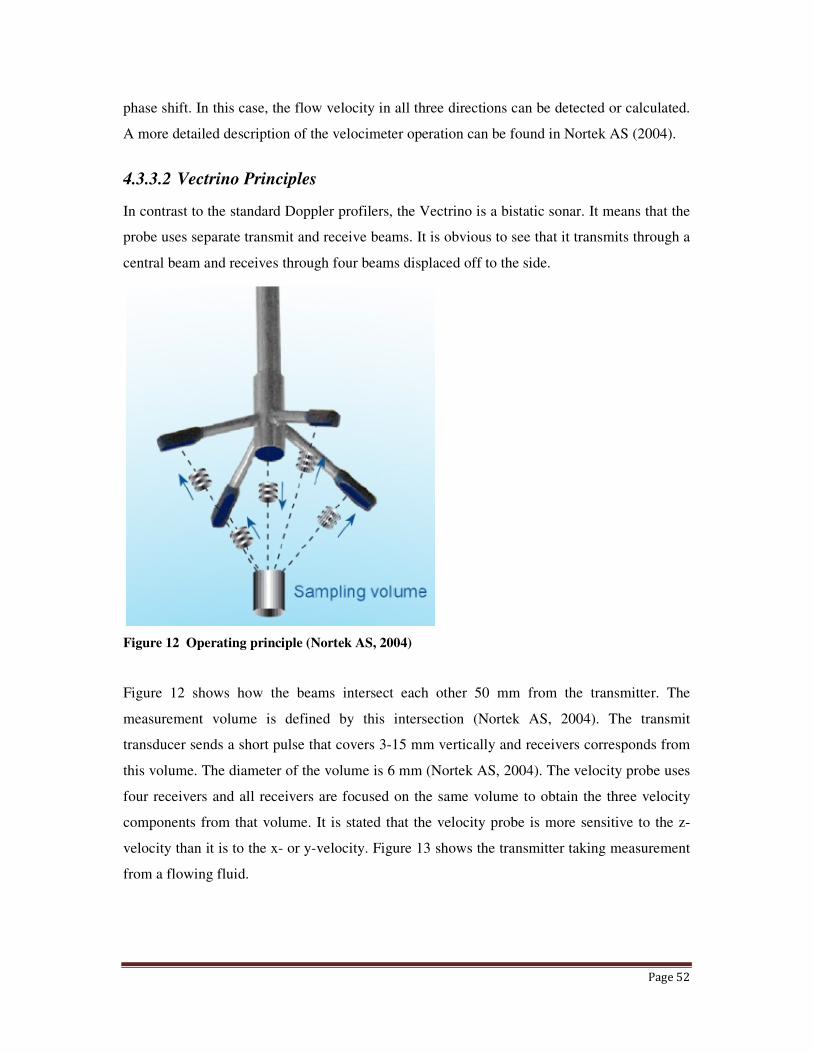
4.3.3.2 Vectrino Principles ................................................................................................................................................ 52
4.3.3.3 Velocity uncertainty ............................................................................................................................................... 53
4.3.4 Calibration of the test flume ..................................................................................................................... 53
4.3.5 Channel for the flume ............................................................................................................................... 61
4.3.6 Test fluid ................................................................................................................................................... 63
4.3.7 Fluid Temperature .................................................................................................................................... 64
4.3.8 Local velocity measurement ...................................................................................................................... 64
4.3.9 Local depth measurement ......................................................................................................................... 64
4.3.10 Experimental procedure ........................................................................................................................... 65
4.3.11 Rheological analysis ................................................................................................................................. 66
4.3.11.1 Rheological modelling ....................................................................................................................................... 69
4.3.11.2 Power law model fit........................................................................................................................................... 69
4.4 SECOND PHASE .................................................................................................................................................. 71
4.4.1 Test flume .................................................................................................................................................. 71
4.4.2 Test fluid ................................................................................................................................................... 76
4.4.3 Fluid density ............................................................................................................................................. 76
4.4.4 Particle size analysis ................................................................................................................................ 77
4.4.5 Experimental procedure ........................................................................................................................... 77
4.4.6 Equilibrium slope testing .......................................................................................................................... 78
4.4.7 Rheological analysis ................................................................................................................................. 80
4.5 ERROR IN EXPERIMENTAL RESULTS ................................................................................................................... 82
4.5.1 Random error analysis ............................................................................................................................. 82
4.5.2 Instrument errors and human errors ........................................................................................................ 84
4.6 SUMMARY ......................................................................................................................................................... 85
5 CHAPTER 5: NUMERICAL MODELLING OF TURBULENT FLOW IN OPEN CHANNELS WITH
SEMTEX ......................................................................................................................................................................... 86
5.1 INTRODUCTION .................................................................................................................................................. 86
5.2 NUMERICAL METHOD ........................................................................................................................................ 87
5.3 BOUNDARY CONDITION ..................................................................................................................................... 88
5.4 MESH GENERATION ........................................................................................................................................... 89
5.5 WALL VISCOSITY AND WALL UNIT ..................................................................................................................... 91
5.5.1 Wall viscosity ............................................................................................................................................ 91
5.5.2 Wall units .................................................................................................................................................. 92
5.6 SESSION FILE ..................................................................................................................................................... 93
5.7 WALL FLUXES AND MODAL ENERGIES ............................................................................................................... 93
5.8 SUMMARY ......................................................................................................................................................... 99
6 CHAPTER 6: EXPERIMENTAL RESULTS AND SIMULATION RESULTS ............................................ 100
6.1 INTRODUCTION ................................................................................................................................................ 100
6.2 INITIAL CALCULATION ..................................................................................................................................... 100
6.2.1 Initial prediction ..................................................................................................................................... 100
6.2.1.1 Wang and Plate data (1996) ................................................................................................................................ 109
6.2.1.2 Kozicki and Tiu shape factor (1967) .................................................................................................................... 111
6.2.2 Entrance length debate ........................................................................................................................... 114
6.3 EXPERIMENTAL RESULTS ................................................................................................................................. 117
6.3.1 Presentation of initial results .................................................................................................................. 117
6.3.1.1 Velocity measurements ........................................................................................................................................ 118
6.3.1.2 Summary of initial observations .......................................................................................................................... 122
6.4 VALIDATION OF SIMULATION RESULTS ........................................................................................................... 125
6.4.1 Use of previous experimental data (Fitton, 2007) .................................................................................. 125
6.4.2 Initial results ........................................................................................................................................... 126
6.4.3 Velocity distribution ................................................................................................................................ 127
6.4.3.1 Coles wake function (1956) ................................................................................................................................. 130
6.4.3.2 Clapp’s velocity profile (1961) ............................................................................................................................ 133
6.4.3.3 Use of Yalin’s roughness height ks (1977) .......................................................................................................... 134
6.4.3.4 Barenblatt’s Power law profile (1993) ................................................................................................................ 136
6.4.3.5 Best fit model ....................................................................................................................................................... 139
Page 12
Page XII
6.4.4 Experimental and simulation results from literature .............................................................................. 143
6.4.4.1 Wallace et al (1972) data .................................................................................................................................... 144
6.4.4.2 Eckelmann (1974) data ........................................................................................................................................ 145
6.4.4.3 Kastrinakis and Eckelmann (1983) data .............................................................................................................. 146
6.4.4.4 Antonia et al (1992) data ..................................................................................................................................... 147
6.4.4.5 Rudman et al (2004) data .................................................................................................................................... 149
6.5 FURTHER DNS INVESTIGATION OF CURRENT SIMULATION RESULTS................................................................ 150
6.5.1 Reynolds number used ............................................................................................................................ 151
6.5.2 Yield stress effect .................................................................................................................................... 154
6.5.3 Flow behaviour index (n) effect .............................................................................................................. 175
6.5.4 Fluid consistency index (K) effect ........................................................................................................... 185
6.5.5 Depth effect ............................................................................................................................................. 199
6.5.6 Side measurements .................................................................................................................................. 204
6.5.7 Finer mesh effect..................................................................................................................................... 207
6.6 SECONDARY FLOW EFFECT .............................................................................................................................. 211
6.7 SUMMARY ....................................................................................................................................................... 231
7 CHAPTER 7: PARTICLE TRANSPORTATION CHARACTERISTICS ..................................................... 232
7.1 INTRODUCTION ................................................................................................................................................ 232
7.2 STOKES NUMBER ............................................................................................................................................. 232
7.2.1 Particle behaviour and Stokes number ................................................................................................... 232
7.3 PARTICLE BEHAVIOUR AND FLOW RELATIONSHIP ............................................................................................ 237
7.3.1 Wall velocity streaks ............................................................................................................................... 237
7.3.1.1 Minimum velocity ................................................................................................................................................ 237
7.3.1.2 Wall velocity streak size ....................................................................................................................................... 240
7.3.1.3 Eddy behaviour and Reynolds number ................................................................................................................ 243
7.3.2 Particle suspension and quadrant analysis ............................................................................................ 250
7.3.2.1 Particle suspension and secondary current ......................................................................................................... 259
7.4 SUMMARY ....................................................................................................................................................... 260
8 CHAPTER 8: CONCLUSION AND RECOMMENDATION ......................................................................... 262
8.1 CONCLUSION ................................................................................................................................................... 262
8.2 RECOMMENDATION ......................................................................................................................................... 264
9 CHAPTER 9: REFERENCE ............................................................................................................................... 266
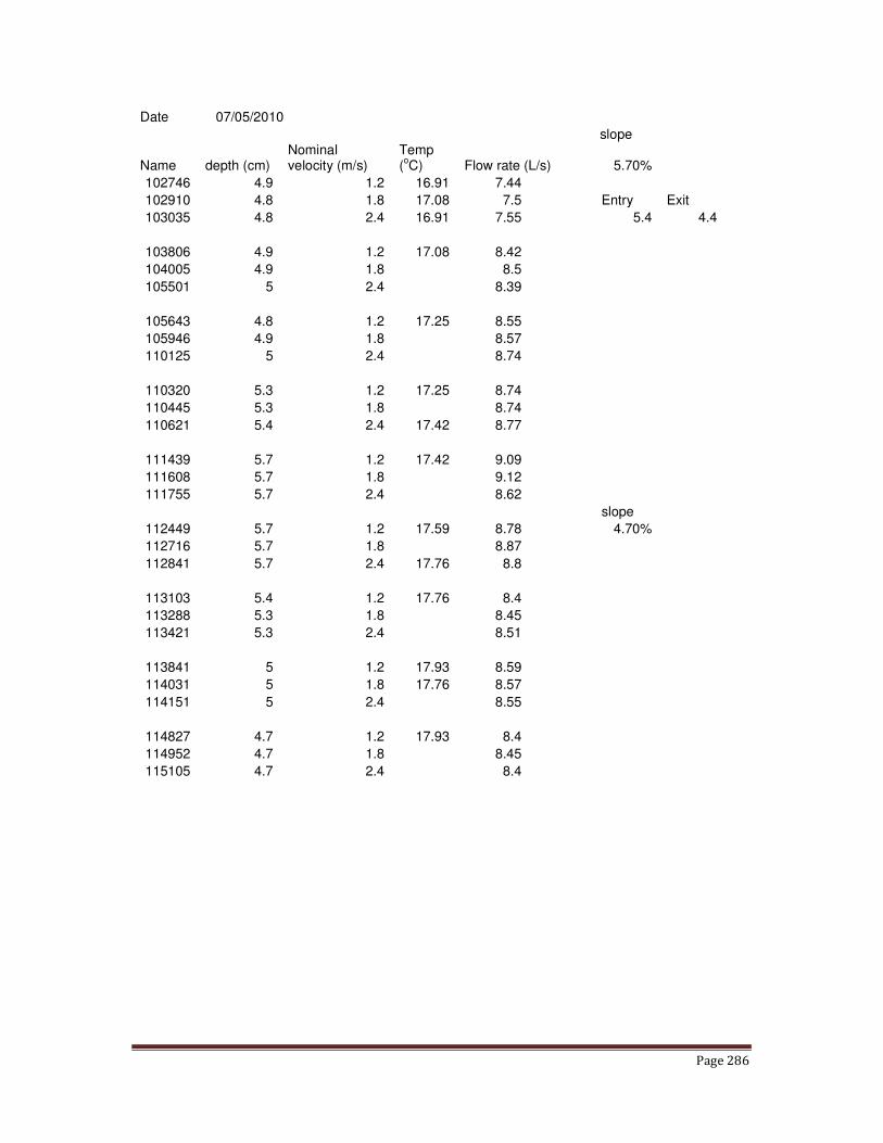
APPENDIX A HIGHETT EXPERIMENTAL DATA .............................................................................................. 283
APPENDIX B TENSOR CONVERTING FROM CARTESIAN FORMAT TO CYLINDRICAL FORMAT ... 301
APPENDIX C MESH SPACING CALCULATION ................................................................................................. 302
APPENDIX D HIGHETT EXPERIMENTAL RHEOLOGICAL DATA AND MODEL FITTING ................... 303
APPENDIX E SMALL FLUME EXPERIMENTS RHEOLOGICAL DATA ........................................................ 311
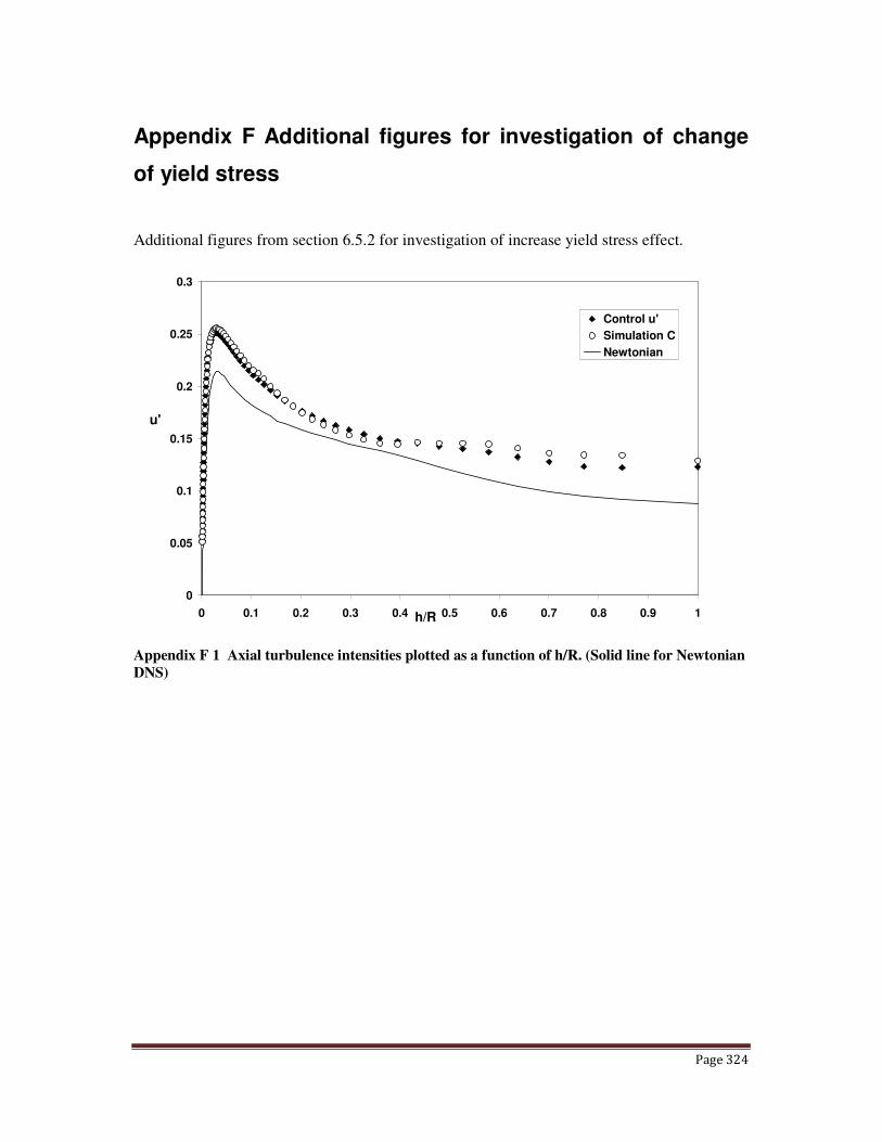
APPENDIX F ADDITIONAL FIGURES FOR INVESTIGATION OF CHANGE OF YIELD STRESS ........... 324
APPENDIX G ADDITIONAL FIGURES FOR INVESTIGATION OF CHANGE OF FLOW BEHAVIOUR
INDEX ........................................................................................................................................................................... 331
APPENDIX H ADDITIONAL FIGURES FOR INVESTIGATION OF CHANGE OF FLOW CONSISTENCY
INDEX ........................................................................................................................................................................... 337
Page 13
Page XIII
LIST OF FIGURES
Figure 1 Types of time-independent flow behaviour (Chhabra and Richardson, 2008) ................... 7
Figure 2 Schematic illustration of non-uniform, axial flow in a flume .......................................... 12
Figure 3 Schematic illustration of the cross-sectional view of open channel flow in a circular flume
..................................................................................................................................................... 12
Figure 4 Definition sketch for steady 2D uniform open channel flow ........................................... 20
Figure 5 Sketch of a representative velocity profile in open channels ........................................... 22
Figure 6 Vector description of secondary currents in open channel by Nezu and Rodi (1985) ...... 27
Figure 7 Quadrants of the instantaneous u'v' plane ....................................................................... 29
Figure 8 Sweep and ejection in turbulent boundary layer (Biddinika, 2010) ................................. 29
Figure 9 Sketch of burst evolution in a flowing liquid layer between a wall and a free surface
(Rashidi and Banerjee, 1988) ........................................................................................................ 36
Figure 10 Near wall structure Re = 3964 (left) and Re = 5000 (right) (Rudman et al, 2001) ......... 42
Figure 11 Closed-circuit test flume .............................................................................................. 51
Figure 12 Operating principle (Nortek AS, 2004) ......................................................................... 52
Figure 13 Photograph of velocity probe in the fluid ...................................................................... 53
Figure 14 Axial velocity profile for nominal velocity range = 0.3 m/s and different transmit lengths
..................................................................................................................................................... 55
Figure 15 Axial velocity profile for nominal velocity range = 1.0 m/s and different transmit lengths
..................................................................................................................................................... 56
Figure 16 Axial velocity profile for nominal velocity range = 2.5 m/s and different transmit lengths
..................................................................................................................................................... 56
Figure 17 Axial velocity profile for nominal velocity range = 4.0 m/s and different transmit lengths
..................................................................................................................................................... 57
Figure 18 Axial velocity profile for nominal velocity range = 2.5 m/s and different transmit lengths
= 1.2 mm and 1.8 mm ................................................................................................................... 58
Figure 19 Photograph of dirt in the flume ..................................................................................... 60
Figure 20 Raw axial velocity data at a rate of 200Hz .................................................................... 61
Figure 21 Photo of top stream end of the semi-circular insert ....................................................... 62
Figure 22 Photo of top stream end of the semi-circular insert 2 .................................................... 62
Figure 23 Photo of downstream end of the semi-circular insert .................................................... 63
Figure 24 A depth measurement ................................................................................................... 65
Figure 25 Photograph of flume entrance ....................................................................................... 66
Figure 26 Rheogram for different samples on the same day .......................................................... 67
Figure 27 Apparent viscosity against shear rate for fluid tested on one day .................................. 68
Figure 28 Rheogram for different samples on the same day but tested on a later date ................... 68
Figure 29 Rheology of CMC in log-log plot ................................................................................. 70
Figure 30 Diagram for small scale flume ...................................................................................... 72
Figure 31 Small scale flume, downstream end .............................................................................. 73
Figure 32 Photograph of flume entrance, taken from the upstream end ......................................... 73
Figure 33 Photograph of calibration tank and holding tank ........................................................... 74
Figure 34 Photograph of inclinometer .......................................................................................... 75
Figure 35 Photograph taken from side of the flume. Note: bed formed on the bottom of the pipe . 75
Figure 36 Particle size curve for sand particles ............................................................................. 77
Figure 37 Plot of equilibrium slope data ....................................................................................... 79
Figure 38 Rheograms for fluid 1307 with the rheological model fit curve inscribed ..................... 80
Figure 39 Apparent viscosity against shear rate of fluid tested ...................................................... 81
Page 14
Page XIV
Figure 40 Boundary condition section in Semtex session file ....................................................... 89
Figure 41 Sample structured 2-D mesh for 43 elements ................................................................ 89
Figure 42 Computer generated 2-D mesh for 43 elements ............................................................ 90
Figure 43 Hand drawing of 2-D mesh for 38 elements.................................................................. 90
Figure 44 Elements with different skewness ................................................................................. 91
Figure 45 Simulation channel geometry ....................................................................................... 92
Figure 46 Part of session file ........................................................................................................ 93
Figure 47 Simulation stress profile over a period of time (converged) .......................................... 94
Figure 48 Simulation stress profile over a period of time (not converged) .................................... 95
Figure 49 Simulation energy profile (converged) ......................................................................... 96
Figure 50 Simulation energy profile (not converged) .................................................................... 96
Figure 51 Instantaneous contours of z plane velocity vectors for the channel flow ........................ 97
Figure 52 Symmetrised z plane velocity u .................................................................................... 97
Figure 53 Symmetrised y plane velocity v .................................................................................... 98
Figure 54 Symmetrised x plane velocity w ................................................................................... 98
Figure 56 Haldenwang et al (2004) locus for predict transition in open channel flow (4.6%
bentonite in 150 mm flume) ........................................................................................................ 102
Figure 57 Predicted relationship for CMC solution A for different slopes. Haldenwang’s locus is
plotted and lies below the data points. ......................................................................................... 104
Figure 58 Predicted relationship for CMC solution B for different slopes. Haldenwang’s locus is
plotted and lies below the data points. ......................................................................................... 105
Figure 59 Predicted relationship for CMC solution C for different slopes. Haldenwang’s locus is
plotted and lies below the data points. ......................................................................................... 105
Figure 60 Rheogram of Ultrez solution tested ............................................................................ 106
Figure 61 Prediction of turbulent region for 0.1% Ultrez solution............................................... 107
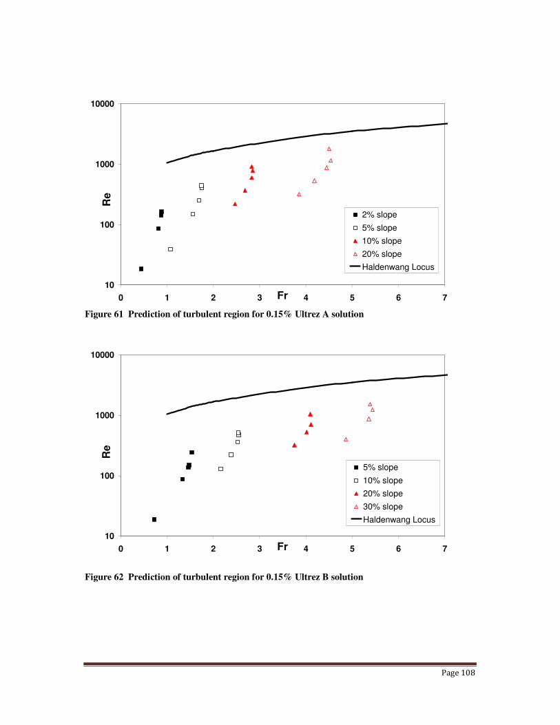
Figure 62 Prediction of turbulent region for 0.15% Ultrez A solution ......................................... 108
Figure 63 Prediction of turbulent region for 0.15% Ultrez B solution ......................................... 108
Figure 64 Combined Plot of Wang and Plate (1996) and calculated points by previous
methodologies Small flume data ................................................................................................. 109
Figure 65 Combined Plot of Wang and Plate (1996) and calculated points by previous
methodologies using large flume data ......................................................................................... 110
Figure 66 Prediction of turbulent region for 0.06% Ultrez solution with Kozicki and Tiu shape
factor .......................................................................................................................................... 112
Figure 67 Prediction of turbulent region for 0.08% Ultrez solution with Kozicki and Tiu shape
factor .......................................................................................................................................... 112
Figure 68 Prediction of turbulent region for 0.1% Ultrez solution with Kozicki and Tiu shape factor
................................................................................................................................................... 113
Figure 69 Prediction of turbulent region for 0.15% Ultrez solution with Kozicki and Tiu shape
factor .......................................................................................................................................... 113
Figure 70 Velocity against depth plot at centreline of the channel for fluid samples 1405 and 1705
with slope equals 4.70% .............................................................................................................. 118
Figure 71 Rheogram for test samples 1405 and 1705 CMC solution at 18oC .............................. 119
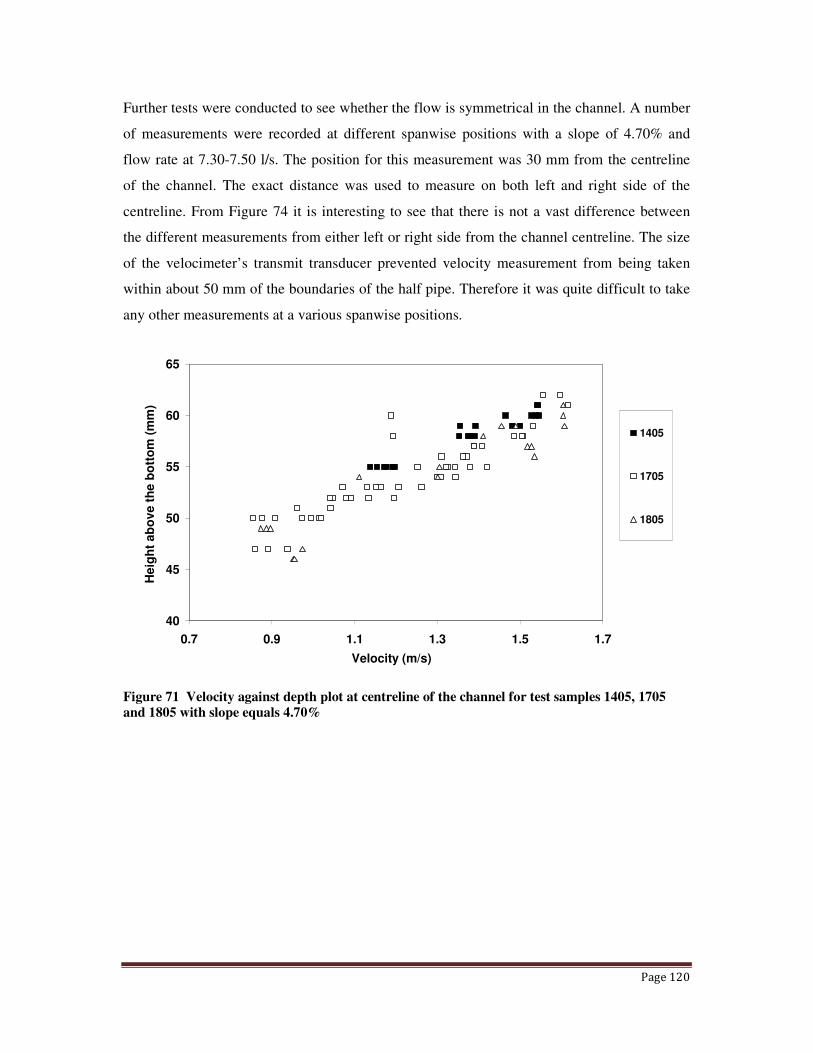
Figure 72 Velocity against depth plot at centreline of the channel for test samples 1405, 1705 and
1805 with slope equals 4.70% ..................................................................................................... 120
Figure 73 Rheogram for test samples 1405, 1705 and 1805 CMC solutions ................................ 121
Figure 74 Velocity against normalised depth plot at centreline of the channel at different flow rate
with slope equals 4.70% .............................................................................................................. 121
Figure 75 Velocity against depth plot at different positions of the channel with slope equals 4.70%
................................................................................................................................................... 122
Page 15
Page XV
Figure 76 Velocity against depth plot at centreline of the channel for test samples 1405, 1705, 1805
and 2405 CMC solution with experimental data of Fitton (2007) ................................................ 124
Figure 77 Splashing at downstream end of the experiment setup ................................................ 124
Figure 78 Air bubbles caused unclearness in the fluid ................................................................ 125
Figure 79 Near wall structure revealed in contours of streamwise velocity, red shows high velocity
regions, blue shows low velocity regions .................................................................................... 126
Figure 80 Instantaneous point velocity at the centre line of the channel ...................................... 128
Figure 81 Experimentally measured velocity profile for slurry Fitton (2007). ............................. 129
Figure 82 Experimentally measured velocity profile in conventional wall units for slurry in
comparison of Simulation results ................................................................................................ 130
Figure 83 Simulation velocity profile in conventional wall units for slurry in comparison of
Simulation results with Coles wake function ............................................................................... 131
Figure 84 Enlarged plot for Simulation velocity profile in conventional wall units for slurry ...... 132
Figure 85 Enlarged plot for Simulation velocity profile in conventional wall units for slurry in
comparison of Simulation results with Coles wake function ........................................................ 132
Figure 86 Simulation velocity profile in conventional wall units for slurry in comparison of
Simulation results with Clapp’s velocity distribution equation .................................................... 134
Figure 87 Simulation mean velocity profile with different roughness value ................................ 136
Figure 88 Simulation velocity profile in conventional wall units for slurry in comparison to
Simulation results with Barenblatt (1993)’s power law velocity profile ....................................... 138
Figure 89 Different simulation velocity profiles with different yield stresses in comparison to
Barenblatt (1993)’s power law velocity profile ............................................................................ 138
Figure 90 Simulation velocity profile in conventional wall units with Clapp’s velocity distribution
equation ...................................................................................................................................... 140
Figure 91 Simulation velocity profile of n = 0.79 and Yang et al (2004) equation ...................... 141
Figure 92 Simulation velocity profile in conventional wall units with Clapp’s velocity distribution
equation and Yang et al (2004) equation ..................................................................................... 142
Figure 93 Simulation velocity profile in conventional wall units with calculated velocity profile 143
Figure 94 Experimentally measured velocity profile in conventional wall units for slurry and in
comparison of Simulation results (Wallace et al, 1972) ............................................................... 145
Figure 95 Experimentally measured velocity profile in conventional wall units for slurry in
comparison to the Simulation results and Eckelmann (1974) data ............................................... 146
Figure 96 Experimentally measured velocity profile in conventional wall units for slurry in
comparison to the Simulation results and Kastrinakis and Eckelmann (1983) data ...................... 147
Figure 97 Simulation velocity profile in conventional wall units for slurry in comparison to the
experimental data (Antonia et al, 1993) ....................................................................................... 148
Figure 98 Simulation velocity profile in conventional wall units for slurry in comparison to the
simulation data (Antonia et al, 1993) .......................................................................................... 149
Figure 99 Simulation velocity profile in conventional wall units for slurry in comparison to
Rudman et al (2004) data ............................................................................................................ 150
Figure 100 Comparison of Haldenwang Reynolds number with Rudman Reynolds number for
4.5% Bentonite in 300 mm flume ................................................................................................ 152
Figure 101 Comparison of Haldenwang Reynolds number with Rudman Reynolds number for
1.0% CMC in 300 mm flume ...................................................................................................... 153
Figure 102 Comparison of Haldenwang Reynolds number with Rudman Reynolds number for
6.0% Kaolin in 150 mm flume .................................................................................................... 154
Figure 103 Mean axial velocity profiles for the turbulent flow of three different Herschel-Bulkley
fluids. The profiles have been non-dimensionalised using the conventional non-dimensionalisation
with the mean wall viscosity taking the place of the Newtonian viscosity .................................... 156
Page 16
Page XVI
Figure 104 Axial turbulence intensities plotted in wall coordinates ............................................ 157
Figure 105 Radial turbulence intensities plotted in wall coordinates ........................................... 158
Figure 106 Azimuthal turbulence intensities plotted in wall coordinates ..................................... 158
Figure 107 Turbulence production plotted in wall coordinates .................................................... 159
Figure 108 Predicted axial velocity at y+ ≈ 8. From top to bottom, Control, Simulation C and
Newtonian simulation. White represents high velocity and black represents low velocity. ........... 160
Figure 109 Contours of instantaneous axial velocity and in-plane velocity vectors ..................... 164
Figure 110 Mean axial velocity profiles for the turbulent flow of three different Herschel-Bulkley
fluids .......................................................................................................................................... 165
Figure 111 Axial turbulence intensities plotted in wall coordinates ............................................ 166
Figure 112 Radial turbulence intensities plotted in wall coordinates ........................................... 167
Figure 113 Azimuthal turbulence intensities plotted in wall coordinates ..................................... 167
Figure 114 Turbulence production plotted in wall coordinates..................................................... 168
Figure 115 Turbulence production of control simulation and simulation C and F plotted in wall
coordinates.................................................................................................................................. 168
Figure 116 Predicted axial velocity at y+ ≈ 8. From top to bottom, Control simulation, Simulation F
and Newtonian simulation. White represents high velocity and black represents low velocity. .... 170
Figure 117 Contours of instantaneous axial velocity and in-plane velocity vectors ..................... 174
Figure 118 Mean axial velocity profile for the turbulent flow of n = 0.75 and 0.79 ..................... 176
Figure 119 Mean axial velocity profile for the turbulent flow of n = 0.85 and n = 0.90 ............... 177
Figure 120 Axial turbulence intensities plotted in wall coordinates ............................................ 178
Figure 121 Radial turbulence intensities plotted in wall coordinates ........................................... 179
Figure 122 Azimuthal turbulence intensities plotted in wall coordinates ..................................... 179
Figure 123 Predicted axial velocity at y+ ≈ 8. From top to bottom, Control, n=0.90, and n=0.75.
White streaks represent high velocity and black streaks represent low velocity. .......................... 181
Figure 124 Contours of instantaneous axial velocity and in-plane velocity vectors ..................... 183
Figure 125 Mean axial velocity profiles for the turbulent flow of two fluids with different K ..... 186
Figure 126 Turbulence production plotted as a function of wall unit .......................................... 187
Figure 127 Predicted axial velocity at y+ ≈ 8. From top to bottom, Control simulation, K +50%,
and K -50%. White represents high velocity and black represents low velocity. .......................... 188
Figure 128 Contours of instantaneous axial velocity and in-plane velocity vectors ..................... 190
Figure 129 Mean axial velocity profiles for the turbulent flow of two fluids with different K values
................................................................................................................................................... 192
Figure 130 Mean axial velocity profiles for the turbulent flow of two fluids with different K values
................................................................................................................................................... 193
Figure 131 Turbulent production plotted as a function of wall unit ............................................. 194
Figure 132 Predicted axial velocity at y+ ≈ 8. From top to bottom, Control simulation, K +30%, and
K -30%. White represents high velocity and black represents low velocity. ................................. 195
Figure 133 Contours of instantaneous axial velocity and in-plane velocity vectors ..................... 198
Figure 134 Mean axial velocity profiles for the turbulent flow of two fluids with different depths
................................................................................................................................................... 201
Figure 135 Predicted axial velocity at y+ ≈ 8. From top to bottom, Control simulation, depth = 0.08
m and depth = 0.06 m. White represents high velocity and black represents low velocity ............ 203
Figure 136 Mean axial velocity profiles for the turbulent flow of with different side measurements
................................................................................................................................................... 204
Figure 137 Mean axial velocity profiles for the turbulent flow at x = 0.04 m .............................. 205
Figure 138 Mean axial velocity profiles for the turbulent flow at x = 0.065 m ............................ 205
Figure 139 Mean axial velocity profiles for the turbulent flow at x = 0.065 m. 10 < y+ <100 ...... 206
Figure 140 Mean axial velocity profiles for the turbulent flow at x = 0.088 m ............................ 206
Page 17
Page XVII
Figure 141 Coordinates of old simulation mesh .......................................................................... 207
Figure 142 Coordinates of finer simulation mesh ....................................................................... 208
Figure 143 Mean axial velocity profiles for the turbulent flow of two different meshes .............. 209
Figure 144 Axial turbulence intensities plotted in wall coordinates ............................................ 210
Figure 145 Radial turbulence intensities plotted in wall coordinates ........................................... 210
Figure 146 Azimuthal turbulence intensities plotted in wall coordinates ...................................... 211
Figure 147 Field experimental velocity (Heays, 2010) against depth plot at centreline of the
channel ....................................................................................................................................... 213
Figure 148 Non-dimensionalised experimentally measured velocity profile ................................ 214
Figure 149 Non-dimensionalised experimentally measured velocity profile (Fitton, 2007) ......... 215
Figure 150 Non-dimensionalised experimentally measured velocity profile, simulation profile and
Yang et al (2004) equation .......................................................................................................... 215
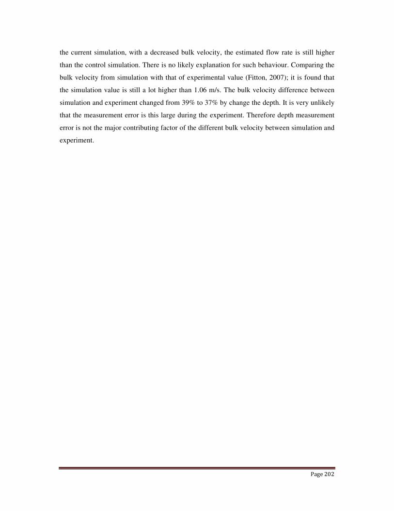
Figure 151 Illustration of velocity measurement (red line) taken at x = 0.04 m ........................... 217
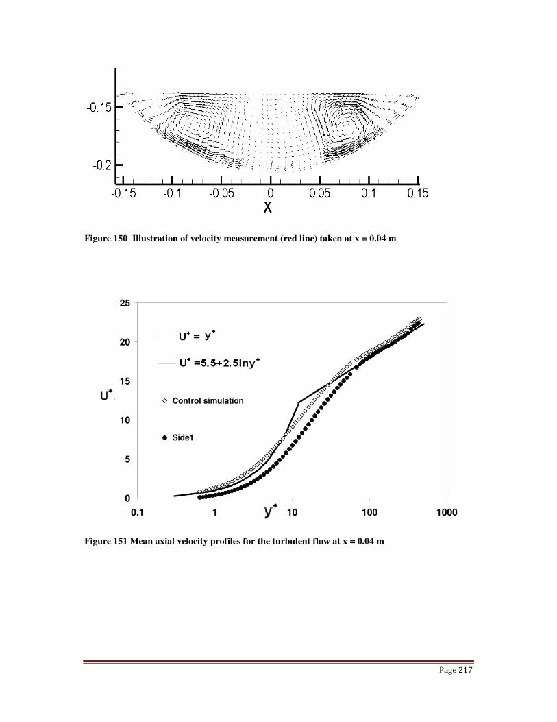
Figure 152 Mean axial velocity profiles for the turbulent flow at x = 0.04 m ............................... 217
Figure 153 Illustration of velocity measurement taken at x = 0.065 m ........................................ 218
Figure 154 Mean axial velocity profiles for the turbulent flow at x = 0.065 m ............................ 218
Figure 155 Illustration of velocity measurement taken at x = 0.088 m ......................................... 219
Figure 156 Mean axial velocity profiles for the turbulent flow at x = 0.088 m ............................ 219
Figure 157 Simulation velocity profile in conventional wall units for slurry in comparison of half
pipe simulation. .......................................................................................................................... 220
Figure 158 Axial velocity contours for half pipe simulation, Newtonian simulation and control
simulation ................................................................................................................................... 223
Figure 159 Velocity vectors for different simulations with different yield stress ......................... 224
Figure 160 Mean axial velocity profiles for the turbulent flow at x = 0.065 m. ........................... 225
Figure 161 Velocity vectors for different simulations with different n ........................................ 226
Figure 162 Velocity vectors for different simulations with different K ....................................... 227
Figure 163 Mean axial velocity profiles for the turbulent flow at x=0.065 m. ............................. 228
Figure 164 Mean axial velocity profiles for the turbulent flow at x=0.088 m. ............................. 228
Figure 165 Velocity vectors for Newtonian simulation ................................................................ 230
Figure 166 Velocity vectors for Newtonian simulation and rectangular duct flow from Yang (2009)
................................................................................................................................................... 230
Figure 167 Stokes number plotted as a function of distance from the wall with different increased
yield stress .................................................................................................................................. 235
Figure 168 Stokes number plotted as a function of distance from the wall with different decreased
yield stress .................................................................................................................................. 235
Figure 169 Stokes number plotted as a function of distance from the wall with two different n
values ......................................................................................................................................... 236
Figure 170 Stokes number plotted as a function of distance from the wall with two different K
values ......................................................................................................................................... 236
Figure 171 Stokes number plotted as a function of distance from the wall with two different K
values with fixed Reynolds number ............................................................................................. 237
Figure 172 Predicted axial velocity at y+ ≈ 8. n = 0.90 and n = 0.75 simulation. White represents
high velocity and black represents low velocity. .......................................................................... 243
Figure 173 Typical eddy in x-y plane at Reynolds number = 12910 ........................................... 245
Figure 174 Typical eddy in x-y plane at Reynolds number = 12910 ........................................... 247
Figure 175 Typical eddy in x-y plane at Reynolds number = 5635 ............................................. 249
Figure 176 Typical quadrant map ............................................................................................... 250
Figure 177 Quadrant analysis at x = 0 cm ................................................................................... 251
Figure 178 Quadrant analysis at x = 20 cm ................................................................................. 252
Page 18
Page XVIII
Figure 179 Quadrant analysis at x = 40 cm ................................................................................. 252
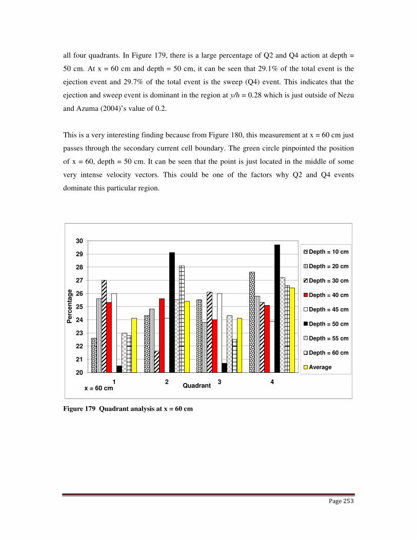
Figure 180 Quadrant analysis at x = 60 cm ................................................................................. 253
Figure 181 Illustration of velocity measurement taken at x = 60 m and depth = 50 cm ............... 254
Figure 182 Quadrant analysis at x = 80 cm .................................................................................. 255
Figure 183 Illustration of velocity measurement taken at x = 80 m and depth = 10 cm ............... 255
Figure 184 Quadrant analysis at x = 90 cm ................................................................................. 256
Figure 185 Quadrant analysis at x = 100 cm ............................................................................... 256
Figure 186 Quadrant analysis at depth = 60 cm .......................................................................... 257
Figure 187 Quadrant analysis at depth = 50 cm .......................................................................... 257
Figure 188 Particle distribution on a horizontal plane at y+ = 3.6 from the wall (Pan and Banerjee,
1996) .......................................................................................................................................... 259
Figure 189 Average velocity vectors for control simulation ......................................................... 260
Appendix D 1 Rheograms for fluid 0405 from Highett experiment ............................................. 303
Appendix D 2 Rheograms for fluid 0705 from Highett experiment ............................................. 304
Appendix D 3 Rheograms for fluid 1105 from Highett experiment ............................................. 304
Appendix D 4 Rheograms for fluid 1405 from Highett experiment ............................................. 305
Appendix D 5 Rheograms for fluid 1705 from Highett experiment ............................................. 305
Appendix D 6 Rheograms for fluid 1805 from Highett experiment ............................................. 306
Appendix D 7 Rheograms for fluid 2405 from Highett experiment ............................................. 306
Appendix D 8 Rheograms for fluid 2805 from Highett experiment ............................................. 307
Appendix E 1 Rheograms for fluid 1307 from small flume experiment......................................... 311
Appendix E 2 Rheograms for fluid 1407a from small flume experiment....................................... 312
Appendix E 3 Rheograms for fluid 1407b from small flume experiment....................................... 312
Appendix E 4 Rheograms for fluid 1507a from small flume experiment........................................ 313
Appendix E 5 Rheograms for fluid 1507b from small flume experiment....................................... 313
Appendix E 6 Rheograms for fluid 1907 from small flume experiment......................................... 314
Appendix E 7 Rheograms for fluid 2007a from small flume experiment........................................ 314
Appendix E 8 Rheograms for fluid 2007b from small flume experiment....................................... 315
Appendix E 9 Rheograms for fluid 2107 from small flume experiment......................................... 315
Appendix E 10 Rheograms for fluid 2607a from small flume experiment..................................... 316
Appendix E 11 Rheograms for fluid 2607b from small flume experiment..................................... 316
Appendix F 1 Axial turbulence intensities plotted as a function of h/R. (Solid line for Newtonian
DNS) .................................................................................................................. 324
Appendix F 2 Radial turbulence intensities plotted as a function of h/R. (Solid line for Newtonian
DNS) .................................................................................................................. 325
Appendix F 3 Azimuthal turbulence intensities plotted as a function of h/R. (Solid line for
Newtonian DNS) ................................................................................................ 325
Appendix F 4 Turbulence production plotted as a function of h/R .............................................. 326
Appendix F 5 Predicted axial velocity at y+ ≈ 8. From top to bottom, Simulation A, B and C. White
represents high velocity and black represents low velocity. ................................. 327
Appendix F 6 Axial turbulence intensities plotted as a function of h/R. (Solid line for Newtonian
DNS) .................................................................................................................. 328
Appendix F 7 Radial turbulence intensities plotted as a function of h/R. (Solid line for Newtonian
DNS) .................................................................................................................. 328
Appendix F 8 Azimuthal turbulence intensities plotted as a function of h/R. (Solid line for
Newtonian DNS) ................................................................................................ 329
Page 19
Page XIX
Appendix F 9 Turbulence production plotted as a function of h/R .............................................. 329
Appendix F 10 Predicted axial velocity at y+ ≈ 8. From top to bottom, Simulation D, E and F. White
represents high velocity and black represents low velocity. ................................. 330
Appendix G 1 Axial turbulence intensities plotted as a function of h/R. (Solid line for Newtonian
DNS) .................................................................................................................. 331
Appendix G 2 Radial turbulence intensities plotted as a function of h/R. (Solid line for Newtonian
DNS) .................................................................................................................. 332
Appendix G 3 Azimuthal turbulence intensities plotted as a function of h/R. (Solid line for
Newtonian DNS) ................................................................................................ 332
Appendix G 4 Predicted axial velocity at y+ ≈ 8. From top to bottom, n=0.90, n=0.85, n=0.79, and
n=0.75. White represents high velocity and black represents low velocity. .......... 333
Appendix G 5 Contours of instantaneous axial velocity and in-plane velocity vectors ................. 336
Appendix H 1 Predicted axial velocity at y+ ≈ 8. From top to bottom, K+20%, K+50%, K-20%, and
K-50%. White represents high velocity and black represents low velocity. .......... 338
Appendix H 2 Contours of instantaneous axial velocity and in-plane velocity vectors ................. 341
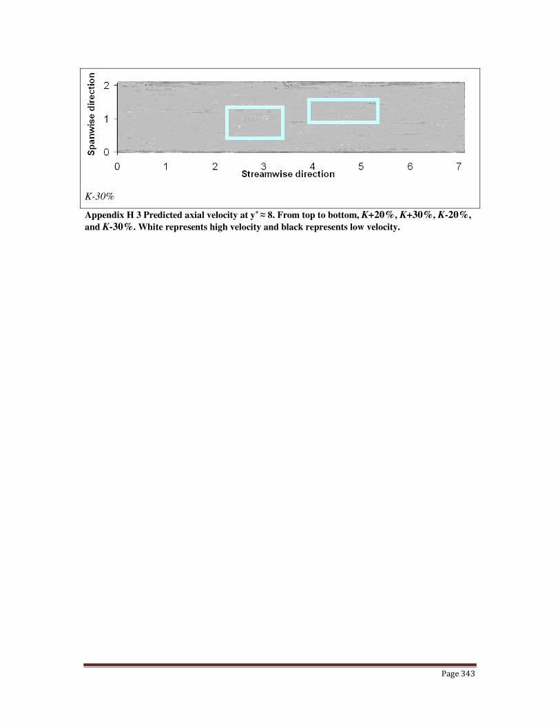
Appendix H 3 Predicted axial velocity at y+ ≈ 8. From top to bottom, K+20%, K+50%, K-20%, and
K-50%. White represents high velocity and black represents low velocity. .......... 343
Appendix H 4 Contours of instantaneous axial velocity and in-plane velocity vectors ................. 346
Page 20
Page XX
LIST OF TABLES
Table 1 Difference between pipe flow and open channel flow ....................................................... 10
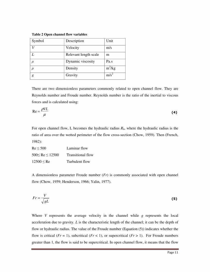
Table 2 Open channel flow variables ............................................................................................. 11
Table 3 Vectrino weak spots ......................................................................................................... 54
Table 4 Comparison between actual velocity and calculated velocity ............................................ 59
Table 5 Power law parameters for the non-Newtonian fluids tested ............................................... 70
Table 6 Power law parameters for the non-Newtonian fluids tested ............................................... 81
Table 7 Summary of first phase experiment flow rate random errors ............................................. 83
Table 8 Summary of mean shear stress and confidence limit statistics for the four different fluids
tested in first phase experiment ..................................................................................................... 83
Table 9 Summary of mean shear stress and confidence limit statistics for the seven different fluids
tested in small flume experiment ................................................................................................... 83
Table 10 Summary of instrument errors and human errors for recorded variables .......................... 84
Table 11 CMC solution parameter .............................................................................................. 101
Table 12 Rheological parameters for Ultrez solution ................................................................... 106
Table 13 Rheological parameters of Ultrez solution .................................................................... 111
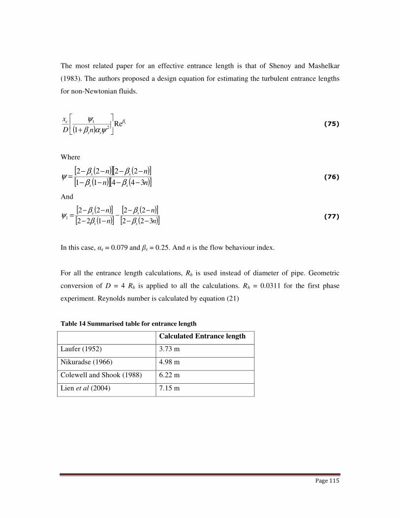
Table 14 Summarised table for entrance length ........................................................................... 115
Table 15 Entrance length calculated by Shenoy and Mashelkar (1983) equation ......................... 116
Table 16 Entrance length calculated by Shenoy and Mashelkar (1983) equation ......................... 116
Table 17 Parameters for simulation 1 .......................................................................................... 126
Table 18 Parameters for simulation ............................................................................................. 155
Table 19 Velocity streak size comparison ................................................................................... 161
Table 20 Velocity streak size comparison ................................................................................... 171
Table 21 Parameters for simulation ............................................................................................. 176
Table 22 Changes in n value in relation to change in Reynolds number ....................................... 184
Table 23 Parameters for simulation ............................................................................................. 185
Table 24 Parameters for simulation ............................................................................................. 191
Table 25 Changes in K values in relation to change in Reynolds number ..................................... 199
Table 26 Parameters for simulation ............................................................................................. 200
Table 27 Minimum velocity in low velocity streaks .................................................................... 240
Table 28 Velocity streak size comparison ................................................................................... 242
Table 29 Random error analysis on flow rate measured on 7/5/2010 ........................................... 298
Table 30 Random error analysis on flow rate measured on 18/5/2010 ......................................... 299
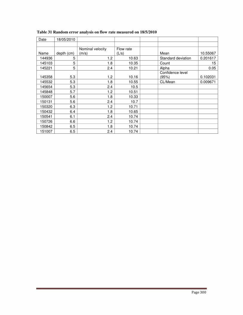
Table 31 Random error analysis on flow rate measured on 18/5/2010 ......................................... 300
Table 32 Rheological data for first phase experimental 0405.1100 .............................................. 308
Table 33 Rheological data for first phase experimental 0405.1200 .............................................. 309
Table 34 Rheological data for first phase experimental 0405.1400 .............................................. 309
Table 35 Rheological data for first phase experimental 0405.1500 .............................................. 310
Table 36 Rheological data for first phase experimental 1307 ....................................................... 317
Table 37 Rheological data for first phase experimental 1407a ..................................................... 318
Table 38 Rheological data for first phase experimental 1507a ..................................................... 319
Table 39 Rheological data for first phase experimental 1907 ....................................................... 320
Table 40 Rheological data for first phase experimental 2007a ..................................................... 321
Table 41 Rheological data for first phase experimental 2107 ....................................................... 322
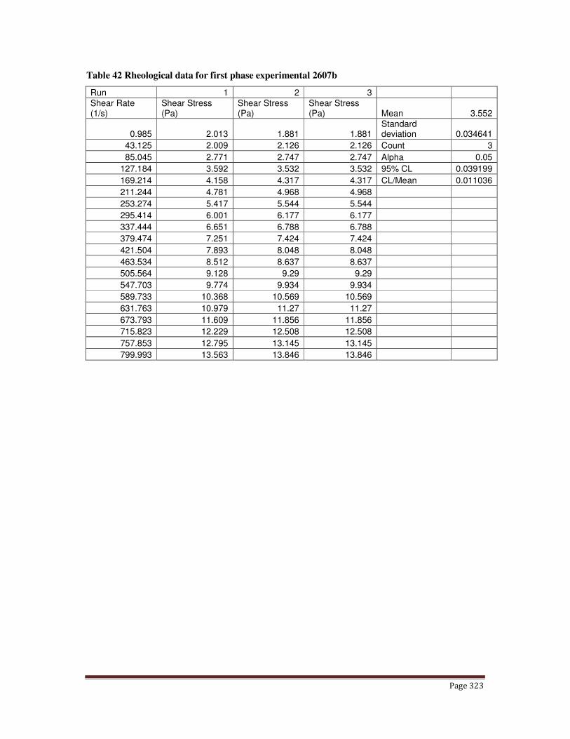
Table 42 Rheological data for first phase experimental 2607b ..................................................... 323
Page 21
Page XXI
NOMENCLATURE
Symbol Description Unit
A Cross sectional area m2
a, b Geometric coefficients from equations (28) and (29)
B Channel width m
Bs Dimensionless property of the flow in the vicinity of the bed
(Yalin, 1977)
C Chezy’s flow resistance
D Diameter m
f Fanning friction factor
F Force N
Fr Froude number
g Gravity, acceleration m/s2
h Height of the channel m
Hb Herschel-Bulkley number
K Fluid consistency index Pa.sn
k Von Karman constant
ks Roughness height m
L Channel length m
M Parameter of velocity distribution equation (60)
n Flow behaviour index
N Number of measurement
P Wetted perimeter m
Pzr Turbulence production
Q Flow rate l/s
r Radius m
Re Reynolds number
Rh Hydraulic radius m
S Slope
St Stokes number
Sm Relative density
Page 22
Page XXII
U Axial velocity m/s
U* Friction velocity m/s
U+ Normalised axial velocity
u0 Average slip velocity at the wall m/s
u’ Axial velocity fluctuation m/s
U, V Average velocity m/s
V Radial velocity m/s
v’ Radial velocity fluctuation m/s
W Azimuthal velocity m/s
w(ξ) Wake function
w’ Azimuthal velocity fluctuation m/s
Y Distance m
y+ Distance from the wall, wall unit
α, β Angle degree
αs, βs Constant in equation (75)
αc Critical value for secondary current generation
αy Factor to predict secondary current in equation (49)
Shear rate s
-1
Г 1-exp (-y+ / 26)
η Apparent viscosity Pa.s
ηr Reference viscosity Pa.s
λ Aspect ratio of the rectangular channel
µ Viscosity Pa.s
ν Kinematic viscosity m2/s
ξ Constant on an isovel on which the velocity is equal to the
mean velocity
П Cole’s wake strength parameter
ρ Density Kg/m3
σ Standard deviation
τ Shear stress Pa
τs Aerodynamic response time
Page 23
Page XXIII
τF Particle response time
τw Wall shear stress Pa
τy Yield stress Pa
φ Function defined by equation (29)
Page 24
Page 1
1 Chapter 1: Introduction
1.1 Purpose and scope
The flow of non-Newtonian fluids in open channels has great implications for mining
industry. When self-formed channels flow at a sufficient gradient or slope, it can generate a
certain level of turbulence. This turbulent behaviour of the transportation material can keep
the particles in suspension. From literature (Chryss et al, 2006) and industrial experience, it is
concluded that if the slope reduces, the intensity of turbulence will decline as well. Therefore
the particles will not be fully suspended in the channel and consequently the channel will
slow its transportation rate and fill with tailing residues.
Particle transportation in the turbulent channel flow is often poorly understood. The addition
of particles in turbulent flow increases the complexity of the turbulent phenomena. The
mechanism governing particle transportation in turbulent flow has been studied in the past;
however they are not completely comprehended. The Centrally Thickened Discharge (CTD)
process is a good example of turbulent channel flow where mine waste is discharged as
thickened slurry at a fixed location, forming low stacks of settled tailings. In this particular
circumstance, the open channels of non-Newtonian suspensions arise spontaneously on the
tailings stacks. A better understanding of the mechanisms operating in the turbulent flow of
non-Newtonian suspensions in the open channels can well improve the operation in financial
terms as well as in sustainability terms.
Over the past fifty years, the study of turbulent non-Newtonian suspension in pipes has
received considerable attention because of its industrial relevance. In the 1960s, experimental
flow visualization techniques were used to investigate the structure of a Newtonian turbulent
boundary layer. In recent times, there has been a significant improvement in understanding
turbulent flow in pipes as a result of improved instrumentation (e.g. Electro-Resistive
Tomography, Particle image velocimetry and Rheometric methods) and computational
techniques (Fluent, CFX and DNS). Although open channel flows are encountered frequently
in industrial and natural circumstances, there has not been the same level of improved
Page 25
Page 2
understanding. Open channels present a complex scenario for analysis because they show
asymmetric velocity and concentration gradients. Moreover, open channels often produce
secondary flows. Usually, open channel flow of water can be described by simple equations
such as Manning’s equation as water has a constant viscosity under isothermal conditions.
However, when water is admixed with a fraction of fine particles, its viscosity becomes
increasingly non-Newtonian. Therefore the velocity distribution in an open channel is usually
difficult to predict.
In open channel flow, a sufficient gradient can generate a level of turbulence that is able to
maintain all the tailings particles in suspension. Shallower gradient will reduce the turbulence
intensity; hence allow more solids to settle in the channel bottom. The channel gradient is
believed to dictate the beach slope of CTD. The CTD process is extremely important to the
mining industry in Australia. With a better understanding of CTD process, there is an
improved possibility to recovering process water, a reduced likelihood of ground water
contamination and more rapid environmental regeneration compared to standard tailing dams.
From previous researches, there is a lack of fundamental understanding about the mechanisms
involved in how a turbulent flow of a non-Newtonian fluid keeps particles in suspension.
1.2 Methodology
Experimental measurement of velocity profiles and turbulence statistics can be used to
determine the state of channel flow. If the rheology of the suspension is known, then
computational simulation can be used to simulate the flow patterns. In earlier years of
research, Kim et al (1987) have simulated turbulent channel flow of Newtonian fluids with
Reynolds number up to 3300. There have been some DNS of the turbulent flow of polymer
solutions as well (Sureskumar et al, 1997). The study considered the drag reduction that arises
in dilute polymer solutions in which shear-thinning behaviour was unimportant.
Dimitropoulos et al (2004) have also used DNS to simulate viscoelastic turbulent boundary
layer flow. It was found that as drag reduction increases, the streamwise velocity fluctuations
are decreased. Furthermore, Rudman and Blackburn (2003, 2006) have used spectral element
method to simulate non-Newtonian flow in pipes. The velocity distribution resulting from the
present approach of adopting the Herschel-Bulkley model showed good agreement in terms of
Page 26
Page 3
shape and magnitude when compared with the experimental data. This indicates that the same
simulation method could also be tested on channel flow with a change of boundary condition.
Experimental data on large scale channels has been obtained for non-Newtonian channel flow
(Fitton, 2007). However, with limitations on equipments, most details of the turbulent
structure are missed, and measurements close to the channel wall are impossible. With the
comparison from both experimental result (Fitton, 2007) and simulation result, more detailed
turbulence characteristics of the flow can be obtained from simulation. Wall velocity streaks
sizes and frequency then can be closely investigated. Therefore it is possible to explore the
possible relationship between rheology of the fluid, turbulence characteristics of the flow and
particle behaviour. Consequently by relating turbulence characteristics to particle behaviour; a
set of new knowledge can be gained from the research. The knowledge will also be significant
for the design and operation of flumes in the process industries.
The study of non-Newtonian suspensions in open channels will provide the additional
fundamental information for understanding the behaviour of self-formed channels in
situations such as CTD stack. The same information will also be applicable to the design and
operation of industrial channels for the transport of mineral suspensions with expected
advantages in management and economic outcomes.
1.3 Aim and objectives
The aim of this project is to understand the underlying phenomena and mechanisms operating
in the turbulent flow of non-Newtonian suspensions in open channels, in particular their
ability to transport suspended particles. It is intended to achieve the following objectives:
• Demonstrate how the rheological characteristics of the continuous medium
carrier fluid influence the transport of solid particles in the suspension
• Carry out modification of existing computational model to describe the non-
Newtonian open channel flow and validate by experimental measurements
• Establish relationships between rheology of the fluid and turbulent
characteristics of the flow
Page 27
Page 4
• Establish relationships between rheology of the fluid and particle suspension in
an open channel flow
1.4 Thesis structure
The work presented here is structured in the following manner:
• Literature Review (Chapter 2). The literature that specifically addresses the topic of
open channel flow, turbulence characteristic of flow, particle interactions and other
relevant literatures.
• DNS studies review (Chapter 3). The literature addresses the previous DNS researches
on turbulent pipe/duct flow and turbulent channel flow.
• Experimental work (Chapter 4)
o Ultrasound velocity probe principles
o Calibration of velocity probe
o Experimental setup
• Numerical modelling of turbulent flow in open channels using Semtex (Chapter 5)
o More detailed numerical method
o Detailed simulation procedures
• Validation of open channel models presented in the literature (Chapter 6). The
simulation results were validated with five different sets of data.
o Presentation of current results
o Validation of simulation results
o Explore the effects of different simulation variables, it includes: Three
different rheological parameters, change of depth, change of measurement
positions, and change of mesh resolution.
o Discussion of secondary current
• Discussion of particle transportation (Chapter 7)
o Establishment of a relationship between fluid rheology and Stokes number
o Establishment of a relationship between fluid rheology and wall velocity
streaks and their sizes
Page 28
Page 5
o Discussion of particle suspension with the assistance of quadrant analysis
o Establishment of a relationship between secondary current and particle
suspension and re-suspension
• A summary of new contributions and findings arising from the work is presented
(Chapter 8)
• Conclusions drawn from the work are presented (Chapter 8)
• Recommendations are presented for future research (Chapter 8)
Page 29
Page 6
2 Chapter 2: Literature Review
2.1 Outline
There is a substantial amount of literature on turbulent flow in pipe and open channel.
Experimental research on turbulent boundary layer and pipe flow has been conducted mainly
in air flow since 1950s using hot wire anemometry. In the late 1960s, experimental flow
visualization techniques were used to probe the structure of a Newtonian turbulent boundary
layer. The basic research on open channel flow has only been investigated from the 1970s.
Since 1980s, laser anemometry has made experimental studies in open channel turbulence
much easier. In recent times, there has been a significant improvement in understanding
turbulent flow in pipes as a result of improved instrumentation (e.g. Electro-Resistive
Tomography, Particle image velocimetry and rheometric methods) and computational
techniques. There is also a large amount of related literature that is extremely relevant to this
work. The literature is presented in the following order:
• Flow behaviour
o Non-Newtonian flow behaviour
• Open channel flow
o Open channel flow categories
o Equations for Newtonian turbulent open channel flow
o Open channel flow review
• Turbulence characteristics of channel flow
o Velocity profile in channel flow
o Secondary current in channel flow
o Quadrant analysis
• Particle interactions
o Particle characteristics
o Turbulence and particle interaction
Page 30
Page 7
2.2 Flow Behaviour
In this section, the flow characteristic of single-phase liquids and pseudo-homogeneous
mixtures is described.
2.2.1 Non Newtonian behaviour
The flow behaviour of a fluid can be classified on the basis of the shear stress-shear rate
relations. If the relationship between shear stress and shear rate is not linear, then the material
is called a non-Newtonian fluid. Sometimes, rheological behaviour of solid-liquid suspensions
is dependent on the interactions between the dispersed components and the suspending
medium which cause the deviation of the shear stress versus shear rate relation from the
linearity observed in Newtonian fluids. Typical tailing slurry may exhibit both yield stress as
well as change in viscosity at different shear rates.
The graphical presentation of some relationships between shear stress and shear rate are
shown in Figure 1.
Figure 1 Types of time-independent flow behaviour (Chhabra and Richardson, 2008)
Page 31
Page 8
2.2.1.1 Non-Newtonian models
Three commonly used rheological models are Power law model, Bingham plastic model and
Herschel-Bulkley model.
Power law model
This model suits a fluid flow that exhibits non-linear behaviour without yield stress. The
equation for the power law model is presented below:
nKγτ &=
(1)
Where τ is the shear stress (Pa), K is the power law consistency index (Pa.Sn), n is a power
and is shear rate applied to the fluid (1/s).
A shear thinning fluid is characterised by an apparent viscosity which decreases with an
increase of shear rate.
Bingham plastic model
This model is the simplest way to describe a flow behaviour with a yield stress. The equation
is as follows:
γττ &Ky +=
(2)
Where τy is the yield stress (Pa), K is the Bingham plastic viscosity (Pa.S) and is shear rate
applied to the fluid (1/s).
This equation is linear and shear stress intercept is the yield stress. It is often used to represent
many concentrated dispersions, emulsions and multiphase mixtures over a range of shear rates
(Bhattacharya, 2001).
Herschel-Bulkley model
Page 32
Page 9
If a yield stress fluid exhibits a non-linear relationship between the shear stress and shear rate,
then the yield pseudoplastic three constant models can be used. The equation is presented
below:
n
y Kγττ &+=
(3)
Where τy is the yield stress (Pa), K is the power law consistency index (Pa.Sn), n is a power
and is shear rate applied to the fluid (1/s). It will be noted that the Herschel-Buckley model
can be easily modified to describe the previously mentioned models.
If τy= 0, the equation becomes the power law equation.
If n = 1, the equation becomes the Bingham equation.
If n = 1, and τy= 0, the equation becomes the Newtonian flow equation.
2.3 Open channel flow
Open channel flow of water is a popular topic and has been studied extensively in the past
(Chanson, 1999; Henderson, 1966). The physical conditions in open channels are quite
different from that in pipes. The cross section of pipes is always round; for open channel the
cross section can be of any shape. Open channel flow tends to be more complicated to predict
because of the free surface which will change with time and space. Moreover, the depth of the
flow, the discharge rate, the slopes of the channel and the free surface are all interdependent.
In addition, an open channel flow is usually driven by gravitational force whereas a pipe flow
is driven by a pressure gradient along with some gravitational effects. Secondary currents
exist in open channel flows, which can cause the maximum velocity to exist somewhere
below the free surface.
Page 33
Page 10
Table 1 Difference between pipe flow and open channel flow
Pipe Flow Open channel flow
Flow driven by Pressure Gravity
Flow cross section Known, fixed Unknown, as flow depth is
unknown
Characteristics flow
parameters
Velocity deduced from
continuity
Flow depth deduced
simultaneously from solving
both continuity and
momentum equations
Specific boundary condition Atmospheric pressure at the
free surface
2.3.1 Open channel flow categories
Open channel flow can be categorised into different types.
• Steady and unsteady flow
Flow in an open channel is steady if the depth of flow does not change or if it can be
assumed to be constant during the time interval under consideration. Therefore in this
category, time is the important criterion.
• Uniform flow and varied flow
If it is a uniform flow, then the depth of the flow is the same at every section of the
channel. The flow is varied when the flow depth varies over the length. A uniform flow
may be steady or unsteady, depending on whether or not the depth changes with time. In
this category, space is the important criterion.
(Chow, 1959)
The open channel flow under investigation for this study is expected to be a steady flow, as
the depth of flow does not change over time. The depth of the flow will be same at every
section of the channel.
Like any fluid mechanical problem, dimensional analysis can play a key role. In open channel
flow, there are a few variables that are needed to describe the transportation of fluid or
suspensions. They are as follows:
Page 34
Page 11
Table 2 Open channel flow variables
Symbol Description Unit
V Velocity m/s
L Relevant length scale m
µ Dynamic viscosity Pa.s
ρ Density m3/kg
g Gravity m/s2
There are two dimensionless parameters commonly related to open channel flow. They are
Reynolds number and Froude number. Reynolds number is the ratio of the inertial to viscous
forces and is calculated using:
µ
ρVL=Re
(4)
For open channel flow, L becomes the hydraulic radius Rh, where the hydraulic radius is the
ratio of area over the wetted perimeter of the flow cross-section (Chow, 1959). Then (French,
1982):
Re ≤ 500 Laminar flow
500≤ Re ≤ 12500 Transitional flow
12500 ≤ Re Turbulent flow
A dimensionless parameter Froude number (Fr) is commonly associated with open channel
flow (Chow, 1959; Henderson, 1966; Yalin, 1977).
gL
VFr =
(5)
Where V represents the average velocity in the channel while g represents the local
acceleration due to gravity. L is the characteristic length of the channel; it can be the depth of
flow or hydraulic radius. The value of the Froude number (Equation (5)) indicates whether the
flow is critical (Fr = 1), subcritical (Fr < 1), or supercritical (Fr > 1). For Froude numbers
greater than 1, the flow is said to be supercritical. In open channel flow, it means that the flow
Page 35
Page 12
can only be controlled by an upstream weir or height control device (Henderson, 1966). For
Froude numbers less than 1, the flow is said to be subcritical. This means that the flow can
only be controlled by downstream devices. Froude number is readily used in Newtonian
flows; however the application for non-Newtonian flow is not fully discovered.
In Figure 2, the flume is inclined at an angle θ from the horizontal plane. Figure 3 shows the
cross sectional area of the flow, the depth of the flow and the angle β, which describes the
location of the free surface relative to the location of the centre of the pipe.
Figure 2 Schematic illustration of non-uniform, axial flow in a flume
Figure 3 Schematic illustration of the cross-sectional view of open channel flow in a circular
flume
For flow in an open channel, the wall shear stress is dependent upon the flume slope angle,
the flow rate and cross-sectional area of flow. The bulk velocity at any location in a steady
flow can be calculated by:
Page 36
Page 13
A
QV =
(6)
The average wall shear stress in the channel can be determined by a force balance on the
system. When uniform flow occurs gravitational forces exactly balance the frictional
resistance forces which apply as a shear stress along the wall. Considering the gravity force
resolved in the direction of the flow is
Gravity force θρ singAL=
(7)
And the boundary shear stress resolved in the direction of flow is
PLwττ =
(8)
In uniform flow these balance
θρτ singALPLw =
(9)
So
θρθρ
τ sinsin
hw gRP
gA==
(10)
The wall shear stress varies along the wetted perimeter of the flow and the value calculated in
Equation (10) is the average shear stress in the open channel.
2.3.2 Equations for Newtonian turbulent open channel flow
There are a number of open channel flow models; some of them are adapted from pipe flow.
A few of the models will be discussed in the next section.
2.3.2.1 Chezy’s equation for channel flow
Most of the existing formulas and theories for pipe flow are not applicable to open channel
flow. As mentioned previously, pipe flow is bounded in all directions by walls which fix the
velocity based on the local cross-section area. In open channel flow, the velocity is not fixed
Page 37
Page 14
as the conditions dictate the depth of flow. Antoine Chezy developed the very first uniform-
flow formula, which is defined as follows (Chow, 1959):
SRCV h=
(11)
Where V is the mean velocity, Rh is the hydraulic radius, S is the slope and C is a factor of
flow resistance called Chezy’s C. This formula applies to turbulent flow. It is also defined as
follows by (Chanson, 1999)
αsinhChezy RCV =
(12)
H. Bazin proposed a formula to predict C (Chow, 1959).
R
mC
+
=
1
6.157
(13)
The value of Bazin constant varies from 0.11 for very smooth cement of planed wood to 3.17
for earth channels in rough conditions (Chow, 1959).
2.3.2.2 Manning’s equation
Robert Manning presented a different equation, which is presented as follows:
2/13/249.1SR
nV h=
(14)
(Chow, 1959)
Where V is the mean velocity, Rh is the hydraulic radius, S is the slope and n is the coefficient
of roughness. This particular formula applies to turbulent flow and is widely used for open
channel flow.
2.3.2.3 Colebrook and White equation
Colebrook and White have designed an equation for pipe flow
+−=
fD
k
f 4Re
51.2
7.3log2
4
1
(15)
Page 38
Page 15
In open channels, the equation can be modified by substituting the diameter with the
hydraulic radius.
+−=
fR
k
f h 4Re
51.2
84.14log2
4
1
(16)
The k value is the equivalent roughness height. This particular equation can be transformed to
an explicit equation in terms of the velocity to be:
+=
αρ
µα
sin32
255.1
84.14logsin32
hhh
hgRRR
kRV
(17)
This equation is used to calculate the flume roughness, and is regarded as one of the more
sophisticated approaches to open channel design (Wallingford and Barr, 1994).
2.3.3 Open channel flow review
The flow of non-Newtonian fluid in open channels is quite common in mineral processing
industry. However, it is not well presented in the literature and textbooks. A significant
amount of research has been applied to the study of the water flow behaviour in open channel.
The other area which attracts research interests is the transportation of sediments in open
channel.
Coussot (1994) investigated flow of concentrated mud suspension in open channels. He used
kaolin as the non-Newtonian suspension which had a particle diameter of less than 40 µm. He
characterised the suspension as a Herschel-Bulkley fluid. The flow behaviour index was fixed
to be 0.333.
The author defined the Herschel-Bulkley number as follows:
n
y
bV
h
KH
=
τ
(18)
Then the author proposed the empirical formula of the average wall shear stress:
Page 39
Page 16
( ) )1(9.0−
+= byw Haττ
(19)
With ‘a’ being the shape factor and differing for different channel shape. For this particular
paper, the wall shear stress equation is only designed for rectangular and trapezoidal channel
shapes. These formulas are only valid for the Herschel-Bulkley fluids and the value of n needs
to be fixed to 0.333. Furthermore the flow needs to be in the laminar region in order to be
valid.
Haldenwang et al (2002, 2003, 2004) investigated a range of non-Newtonian fluid flows in
open channel. Laminar and transitional flows were both achieved. The author used different
concentrations of CMC solutions, kaolin and bentonite suspensions in the experiment. He
characterised the CMC solution as a power law fluid, the kaolin suspension as a Herschel-
Bulkley fluid and bentonite suspension as a Bingham fluid. The author conducted
experiments in three different sizes of rectangular flumes, which were 75 mm, 150 mm and
300mm wide. The 75 mm flume was 4.5 m long and the 150 mm and 300 mm flumes were 10
m long. The author used five different slopes in the experiments, from 1 to 5 degrees.
The author defined Reynolds number as follow:
n
h
yR
VK
V
+
=2
8Re
2
τ
ρ
(20)
He modified the Slatter’s Reynolds number to open channel flow (Slatter, 1995) by
substituting the pipe diameter with hydraulic radius.
For power-law fluids, the equation reduces to:
n
hR
VK
V
=
2
8Re
2ρ
(21)
For the Bingham fluids the equation reduces to:
Page 40
Page 17
+
=
h
yR
VK
V
2
8Re
2
τ
ρ
(22)
Further, Haldenwang (2003) developed a new model for predicting the onset of transition and
the onset of turbulence for non-Newtonian open channel flow. The author stated that the flow
behaviour could be characterised by the Froude number and the Reynolds number.
Haldenwang (2003) plotted Reynolds number against Froude number to establish the
correlation between the two dimensionless numbers. He found that there is a linear
relationship between the tested slopes. Then the linear relationship was plotted against the
apparent viscosity. A critical Reynolds number was established by using the Froude number
to predict the onset of transition. The Reynolds number was found to have a linear
relationship with the Froude number for an apparent viscosity at 100 s-1
.
This critical Reynolds number is as follows:
( )( ) ( )( ) 75.0
100
21.0
100 11
71200Re
−−
+=sappsapp
c Frµµ
(23)
To predict the onset of transition the following procedure is followed:
• Select the Reynolds number
• Calculated f with laminar flow friction factor, which is: f = 16/Re
• Guess the flow depth
• Calculate the velocity using Darcy friction factor equation 2
2
V
gSRf h=
• Calculate Re using equation (20).
• Optimise the flow depth until the two Reynolds numbers are the same
• Calculate the Froude number
• Calculate the Re transition using equation (23)
• Optimise the flow depth until Re is the same as Rec for onset of transition
Page 41
Page 18
To predict the onset of turbulence, the author used similar procedure as for the onset transition
prediction. The only difference is that the linear relationship was at an apparent viscosity at
500 s-1
. This critical Reynolds number is as follows:
( )( ) ( )( ) 65.0
500
52.0
50011
108105Re
−−
+=sappsapp
c Frµµ
(24)
To determine the onset of turbulence, the procedure is as follows:
• Complete the first seven steps used when predicting the onset transition as above
• Calculate the critical turbulent Reynolds number using equation (24)
• Optimise the depth until Re is the same as Rec for onset of turbulence
However, there is no mention of coarse particle transportation in laminar or turbulent flow in
any of those works. Moreover the author did not include any turbulence characteristics in the
paper and there is no measurement of local velocities as well. The prediction of transition and
turbulence is purely based on Reynolds number and Froude number relationship. In Chapter
6, these methods will be used for the prediction of turbulence.
The shape factors were first defined by Straub et al (1958) in their open channel investigation.
Kozicki and Tiu (1967) investigated the effect of shape in laminar flow in open channels
further in their work. They proposed an analytical method by which frictional effects resulting
from non-Newtonian fluid flow can be predicted in ducts of arbitrary cross-section (Kozicki
and Tiu, 1967). Additional relevant research included the work of Metzner and Reed (1955)
and Straub et al (1958) who attempted to correlate data and create a method for predicting
wall shear stress and turbulent transition for non-Newtonian fluids in ducts of different cross
sections.
Kozicki and Tiu (1967) showed that the method can be applied to open channel gravity flows
with the following flow conditions.
1. Incompressible, time independent, non-Newtonian fluid
2. Isothermal, stead, one-dimensional, laminar, gravity flow
3. No-slip at channel walls
4. Zero shear free surface
Page 42
Page 19
5. Flow is uniform (free surface height does not change with axial position), no ripples or
waves
6. Smooth channel wall
Kozicki and Tiu (1967) proposed a Reynolds number for a power-law fluid in rectangular
flume as follows:
( )n
n
n
h
n
n
bnaK
RuU
+
−=
−
−
3
2
0
2
Reρ
(25)
This Reynolds number includes the shape factors ‘a’ and ‘b’. With a semi-circular open
channel, a = ¼ and b = ¾, and for rectangular open channel a = 0.21 and b = 0.68.
For a rectangular open channel ‘a’ and ‘b’ are as follows:
( )( ) ( )
++
−−
+= ∑
∞
033
2
2
12cosh
1
12
1321
12
1
πλπλ
λnn
a
n
(26)
With
hB/=λ
(27)
[ ]13 −= ϕab
(28)
Where
( )( ) ( )
( )( )
+
+−
++
−−
=
∑
∑
∞
∞
πλλπ
πλπ
ϕ
2
12tanh
12
111921
2
12cosh
1
12
1321
055
033
n
n
nn
n
(29)
These shape factors however have not been tested against any valid experiment dataset. In
fact, Kozicki and Tiu’s shape factor can only predict the flow rate and maximum velocity in
Page 43
Page 20
laminar flow of an incompressible, time-independent non-Newtonian fluid in a straight open
channel (Kozicki and Tiu, 1967). In Chapter 5, these models will be tested with data compiled
for this thesis.
2.4 Turbulence characteristics of channel flow
Velocity distribution and turbulence characteristics in open channel flow have been studied
theoretically and experimentally by many researchers. The following section reviews some
interesting aspects of turbulence research in open channels.
2.4.1 Velocity profile in channel flow
In open channel flow, the velocity is not constant with depth. It usually increases from zero at
the invert of the channel to a maximum value close to the surface. The velocity difference
results from the resistance to flow at the bottom and sides of the channel. Theoretical
exploration used the statistical theory of turbulence for uniform and fully developed flows in
wide open channels. Some of the most definite data in 2-D open channel flow are velocity
distributions. All the flows referenced in this section are fully developed turbulent flows.
Figure 4 Definition sketch for steady 2D uniform open channel flow
Page 44
Page 21
Figure 4 shows the coordinate system in open channel flows. As shown in the figure, u, v, and
w denote the components of mean velocity; u', v' and w' denote the velocity fluctuations.
Turbulent flow along a wall can be considered to consist of three regions, characterized by the
distance from the wall. The very thin layer next to the wall where viscous effects are
dominant is the viscous (or laminar or linear or wall) sublayer. Next to the viscous sublayer is
the buffer layer, in which turbulent effects become significant, but the flow is still dominated
by viscous effects. Above the buffer layer is the outer (or turbulent) layer where turbulent
effects dominate over molecular diffusion effects (Cengel and Cimbala, 2006).
Experimental evidence shows that all wall shear turbulent velocity profiles, such open
channel flow and boundary layer flows can be divided into two regions (Coles, 1956). These
two regions are: an inner region where turbulence is directly affected by the bed; and an outer
region where the flow is only indirectly affected by the bed through its shear stress. The inner
region can be divided into a viscous sublayer, a buffer layer and an overlap. Also the outer
region can be further divided into the overlap and a wake layer. In summary, the flow domain
in a wall shear turbulence can be divided into four layers: viscous sublayer, buffer layer,
overlap layer (or intermediate layer), and wake layer, shown in Figure 5.
Page 45
Page 22
Figure 5 Sketch of a representative velocity profile in open channels
The mean velocity distribution for fully developed turbulent flow could be expressed by the
logarithmic velocity distribution equation of von Karman-Prandtl (Cengel and Cimbala,
2006):
( ) Ayk
U += ++ ln1
(30)
Where
ν
*yUy =+
, *U
UU =+
and ρτ /* wU =
(31)
In equation (31), where U* is the friction velocity, A is a constant of integration and k is the
von Karman constant. A and k values are determined experimentally to be about 5.29 and 0.41
respectively (Nezu, 2005), regardless of the Reynolds number and Froude number. Nezu and
Nagakawa (1993) reviewed results in other smooth-wall-bounded shear flows and found the
following values for the constants in the log-law profile: k = 0.41 and A = 5.0 in boundary
layers by Coles (1968); k = 0.41 and A = 5.17 in closed channel flow by Dean (1978). The
von Karman constant is concluded to be 0.41 irrespective of flow configuration. However,
Page 46
Page 23
constant A may weakly depend on main flow properties but is nearly constant. i.e. between A
= 5.0 - 5.3 on smooth beds. It is seen that the constants for ‘plane’ boundaries do not seem to
differ much from those found for channel of circular cross section. It is indicating the
similarity of the flow in the near-wall region of both cases.
In the viscous sublayer,
++ = yU
(32)
Equation (32) is the ‘log-law’ and is valid only in the wall region of the flow. Equations (30)
and (32) are the ‘law of the wall’. It is viewed as a universal velocity profile for turbulent
flow in pipes and is also readily used in channel flow cases.
Van Driest (1955) provides a different A and k value for the logarithmic velocity distribution
equation.
( ) 24.5log174.0
110 += ++ yU
(33)
In this case, the author used a log10 rather than the natural log.
However, in buffer layer, there is no analytical solution available. Clapp (1961) proposed a
velocity distribution equation for power law fluid which included an equation for buffer layer
Viscous
sublayer
( ) nyU
/1++ = ,n
y 50 << +
(34)
Buffer sublayer 05.3ln
5−= ++ y
nU , 25
++ << yyn
(35)
Turbulent layer Hy
n
GU += ++ ln , 2
++ > yy (36)
Where G and H are empirical constants to be obtained by experiment. y+
2 = 30 is used for
Clapp’s (1961) paper and also in Chapter 6 of this work. The observed velocity distributions
by the author were correlated by the equation:
Page 47
Page 24
ny
nU
8.3ln
78.2+= ++
(37)
Investigations (Coles, 1956) have shown that the deviation of the velocity distribution in the
outer region of open channel flows from the log-law can be accounted for by adding a wake
function.
( )ξwAyk
U ++= ++ ln1
with ( )
Π= ξ
πξ
2sin
2 2
kw
(38)
Where w(ξ) accounts for the deviation and termed the wake function, and П is termed the
Coles’ wake strength parameter. Equation (38) is known as ‘the velocity defect law’ or ‘the
log-wake law’. Experiments conducted by Eckelmann (1974) and Nezu (2005) showed that П
is about zero at low Reynolds number < 500. At small values of Re greater than 500, П
increases rapidly with Re and it remains nearly constant, i.e. П =0.2 for Re > 2000.
Barenblatt (1993) introduced a specific power law for the velocity profile in pipe flow. This
law fits data in the inner part of the wake region and the outer part of the log region.
α++ = AyU
(39)
( ) ddA Reln3
1
2
5Re +=
(40)
( )d
dReln2
3Re =α
(41)
Where Red = VD/υ. The Red is based on the average pipe velocity V and the pipe diameter D =
2r. However, it is uncertain that if this power law fits for open channel flow.
Yalin (1977) introduced a set velocity distribution equation in turbulent flow with roughness
of the channel considered. The author stated that:
• if U*ks/υ < ≈ 5, then the velocity distribution is
s
s
Bk
y
kU +=+ ln
1, 5.5
*ln5.2 +=
νs
s
kUB
(42)
• if U*ks/υ > ≈ 70, then the velocity distribution is
Page 48
Page 25
s
s
Bk
y
kU +=+ ln
1, 5.8=sB
(43)
Where U* is the friction velocity, ν is the kinematic viscosity. ks is Nikuradse’s original
uniform sand grain roughness, it represents the equivalent sand roughness for any type of
rough surface. B is a dimensionless property of the flow in the vicinity of the bed; in general,
it must be a certain function of U*ks/υ. Kirkgoez (1988) conducted experiments with different
rough surfaces in open channel flows. Experiments were performed in a glass-walled channel
about 12 m long. Laser-Doppler anemometer was used to measure the flow velocities. The
author found that on rough beds, the law-of-the-wall fits quite well for different roughnesses.
However, the velocity-defect distribution shows some scatters.
Chiu and Tung (2002) proposed a method to predict the position of maximum velocity under
water surface. The author derived the following velocity distribution equation:
( )
−+=
max
max 11lnξ
ξMeM
UU
(44)
In which U = velocity; Umax = maximum velocity in a channel cross section; M = parameter;
ξmax = maximum value of ξ and occurs at the location of Umax; and ξ = constant on an isovel
on which the velocity is equal to U. ξ/ ξmax is equivalent to the probability of velocity,
randomly sampled in a channel section, being less than or equal to U. M can be calculated by
the ratio of the mean and maximum velocity:
Me
e
U
UM
M 1
1max
−−
=
(45)
ξ can be expressed as a function of y:
−
−
−
=
−−
−=
Depth
h
Depth
y
Depth
h
Depth
y
hDepth
y
hDepth
y
1
1exp
1
1expξ
(46)
In which y = vertical distance from the bed. There are three cases for ξ, but only the following
one is considered to be applicable for this research.
Page 49
Page 26
• The maximum velocity Umax occurs at a vertical distance h below the water surface, or
y = Depth - h. In this case, h > 0 and ξmax as well as Umax occurs at y = Depth - h.
therefore
−−
−==
hDepth
y
hDepth
y1exp
max
ξξ
ξ
(47)
Since h represents the distance of Umax from the water surface, the upper limit of h/Depth is
unity. In Chapter 6, these velocity profile equations will be tested with data compiled for this
thesis.
2.4.2 Secondary current in channel flow
In 1878, Francis (cited in Gulliver and Halverson, 1987) first hypothesized the secondary
currents concept. His explanation for secondary current was the depression of the point of
maximum velocity from the free surface. Nikuradse (cited in Yang, 2009) first made the
observations of secondary currents that appeared near the corners of the duct cross section.
There are two kinds of secondary currents described in the literature. If the flow is not
uniform in the streamwise direction, streamwise vorticity is generated by vortex stretching
(Nezu and Nakagawa, 1993). Secondary currents generated by this particular mechanism are
called ‘secondary currents of Prandtl’s second kind’. The first kind of secondary current has
been widely investigated in curved channels and river ways. The other type of secondary
currents is caused by the sidewall effect. These secondary currents of Prandtl’s second kind
are often termed turbulence-driven secondary currents. This particular secondary current can
not arise in laminar straight channel flow (Nezu, 2005). The presence of secondary current
displaces considerably the velocity contours.
In fact the secondary currents in open channel flows remained comparatively unknown until
recently. The most important feature is that the maximum velocity appears not at the free
surface, but just below the free surface in open channel flows. It is also suggested by Nezu
and Nakagawa (1993) that this phenomenon is called the “velocity-dip”, and it is peculiar to
open channel flows. According to Nezu and Nakagawa (1993) and Nezu (2005), a secondary
current is where the lower velocity/momentum material has been dumped into the high
velocity/momentum region. Therefore there is a dip in the axial velocity profile after
Page 50
Page 27
maximum velocity has been reached. This happens regularly in non circular channel flow.
Only this second kind of secondary currents is studied in the present research.
Nezu and Rodi (1985) used a two-colour LDV system to measure the longitudinal velocity
and vertical velocity in an open channel. Figure 6 shows the velocity vectors of the secondary
currents measured by Nezu and Rodi (1985) in a narrow open channel. It is quite obvious that
a strong vortex occurs near the free surface. This vortex is called the ‘free-surface vortex’, and
its pairing vortex near the bottom of the channel is called ‘bottom vortex’. This free-surface
vortex is much stronger than the bottom vortex. Free-surface vortex transports momentum
and energy from the side of the channel toward the centre of the channel. The strong down
flow that occurs at the channel centre causes the so called velocity dip as momentum is
transported from the free surface to mid-depth.
Figure 6 Vector description of secondary currents in open channel by Nezu and Rodi (1985)
Einstein and Li (1958) first deduced the equation of relation between the longitudinal
vorticity and Reynolds shear stress. It is quite accepted that secondary flows are induced by
the imbalance of normal Reynolds shear stress. In Gessner (1973), the author stated that the
anisotropy of turbulent normal stresses, 2ν and
2w , did not play a major role in the generation
of secondary currents. Knight and Sterling (2000) conducted experiments in circular conduits,
with and without a smooth flat bed, and flowing partially full. The author discovered that the
Page 51
Page 28
secondary current appeared in both near the free surface and in the corner regions, particularly
when a deposited sediment bed is presented.
In Nezu (2005), the author summarised that the velocity-dip phenomenon occurs if b/h ≤ αc .
The value of αc is equal to 5 or slightly larger. It is then classified into two categories:
• Narrow open channels, b/h ≤ αc . Corner flows are generated in flows because the side
wall produces anisotropy of turbulence in the same manner as for closed-channel
flows. The velocity-dip is also caused by the free-surface effect whereby the
anisotropy of turbulence differs from that for closed-channel flows (Nezu, 2005).
• Wide open channels, b/h > αc. The side-wall effect disappears. But if any spanwise
variation of bed shear stress occurs that is periodic, cellular secondary currents are
generated. However, it is not investigated in this research.
Yang et al (2004) proposed a velocity distribution profile for secondary current in rectangular
open channel as follows.
−+
=+
h
y
ky
y
kU
o
1lnln1 α
(48)
Where αy is the factor to predict secondary current given by
−=
h
By
2exp3.1α
(49)
In αy = 0, the above equation will become the classical log law. The second term on the RHS
plays an important role in the outer region. However, it is negligible in the inner region as
ln(1-y/h) ≈0. This will be tested in the Results section.
2.4.3 Quadrant analysis
This particular method is used in various journal papers to investigate the Reynolds stress
structures and features of the large eddy. In this research, quadrant analysis is used as a tool to
quantify the near boundary behaviour of the fluid.
Page 52
Page 29
The quadrant analysis technique is introduced by Willmarth and Lu (1972) for a turbulent
boundary layer. This technique sorts out contributions to the Reynolds shear stress u'v' into
quadrants of the u-v plane. The largest positive contributions to the turbulent energy were
provided by the ejection (u'<0, v'>0) and sweep quadrants (u'>0, v'<0), while small and
negative contributions were made by the interaction quadrants (u'<0, v'<0 and u'>0, v'>0).
The first quadrant u'>0, v'>0, contains outward motion of high-speed fluid. The second
quadrant u'<0, v'>0 contains the motion associated with ejections of low-speed fluid away
from the wall. The third quadrant u'<0, v'<0 contains inward motion of low-speed fluid. The
fourth quadrant u'>0, v'<0 contains an inrush of high-speed fluid; this is usually referred to as
the sweep event (Kim et al, 1987).
Figure 7 Quadrants of the instantaneous u'v' plane
Figure 8 Sweep and ejection in turbulent boundary layer (Biddinika, 2010)
Page 53
Page 30
In Wallace et al (1972), the author used Hot-film measurement to measure Reynolds stress in
a full developed channel flow. The Reynolds number based on the width of the channel and
the centre-line velocity is 7150. This is equivalent to a pipe Reynolds number of 11000
(Wallace et al, 1972). Under these turbulent conditions, the author concluded that turbulent
energy dissipation is associated with the Reynolds stress producing motions i.e. sweep and
ejection. However, the author did not comment on the actual position of sweep and ejection.
The investigation is been limited by equipment measuring ability. It has been discovered in
Kim et al (1987) that the ejection event dominated away from the wall region whereas the
sweep event dominated in the wall region. In Kim et al (1987)’s study, the author only used
direct numerical simulation to produce Reynolds stress in a turbulent channel flow.
Rajagopalan and Antonia (1982) conducted X-wire/cold wire arrangement to measure
velocity fluctuations in a wind tunnel. Their quadrant analysis technique is based on
instantaneous products of longitudinal, normal velocity fluctuations and the temperature
fluctuation. They found that the frequency of ejections is nearly equal to sweeps. Yet, they
also did not comment on the place where sweep or ejection most likely to happen.
Antonia and Browne (1987) investigated the average momentum and heat transfers in the
self-preserving region of a turbulent wake. Similar to Rajagopalan and Antonia (1987) they
used X-wire/cold wire technique to measure velocities in a wind tunnel. The main focus of
this research is on the vortex motion of a turbulent wake. In this case, the author identified
ejections with the outer downstream part of a spanwise vortex and sweeps with the inner
upstream part of the same vortex.
Shvidchenko and Pender (2001) presented a paper on the macro-turbulent structure of open
channel flow. The author conducted the experiment with water in an 8 m long rectangular
flume. They used SONTEK acoustic Doppler velocimeter to measure the velocity of the fluid.
They also used a flow visualization technique to study the large scale turbulent structure of
the flow. They used quadrant analysis and ADV to show the existence of sweeps and
ejections in the channel. It is concluded that the upwelling (ejection) and high forward speed
downwelling (sweep) fluid motions significantly increase the local Reynolds stress. This
finding is parallel to Kim et al (1987)’s conclusion. Moreover, Shvidchenko and Pender
Page 54
Page 31
(2001) stated that if the sweep and ejection motion are strong enough, then the motion could
suspend the bed particles.
Klipp et al (2006) used quadrant analysis on atmospheric surface layer. They deployed an
array of sonic anemometers mounted on five towers in Oklahoma City. The author studied the
turbulent transport and dispersion in the atmospheric boundary layer within an urban
environment. They actually focused only on the turbulent momentum transport on wind
vectors. Moreover, the authors did not put any emphasis on sweep and ejection, but on
quadrant 1 and quadrant 3 motion instead.
Robinson (1991) stated that the majority of the turbulence production in the entire boundary
layer occurs in the buffer region. The near wall turbulence production process is considered to
be an intermittent, quasi-cyclic sequence. It is usually referred to as ‘bursting’. It has
described as ‘violent breakup of a low-speed streak after lifting’, and ‘shear-layer interface
sandwiched between an upstream, high-speed sweep and a downstream, low-speed ejection’
(Robinson, 1991). Most of the definitions about bursting process describe it as a highly
intermittent, explosive event. It is a very satisfying concept for the production of turbulent
motion.
Yalin (1977) also mentioned ‘bursting’ as an ‘observable chain of events’. The total chain of
the events mentioned is referred to as the ‘burst’. It seems that the bursting process is
regenerative. I.e. a ‘recirculation cell’ is formed by the sweep action, then it would
disintegrate into a multitude of smaller eddies. Therefore the path of a module or a macro-
turbulent eddy should end just on the downstream side of the location where the path of the
next module begins. This is a vast area and is extremely relevant with regards to particle
transportation in channels. In the next section, the interactions between particles and turbulent
structure will be discussed in details.
2.5 Particle interactions
From the literature, there are two issues of fluid dynamics which are poorly understood:
turbulence and two-phase flow. This section will review the interaction between these poorly
understood areas. In the coming section, only the effect of the particles on the turbulence in a
boundary layer will be discussed in some depths.
Page 55
Page 32
2.5.1 Particle characteristics
2.5.1.1 Stokes number
Crowe et al (1993) published some parameters which affect the particle dispersion in large
scale and organized structures. The authors proposed a Stokes number defined as:
F
sStτ
τ=
(50)
Where τs is the aerodynamic response time of a particle and τF is the time associated with the
motion of the large scale structure. The particle response time is the time it takes for the
particle to respond to changes in the local flow velocity. It depends on the particle’s radius
and density (Hogan and Cuzzi, 2001). The aerodynamic response time is scaled as:
µρ
ρτ
f
p
s
d
18
2
=
(51)
Where ρp is the material density of the particle, d is the particle diameter and µ is the dynamic
viscosity of the carrier fluid. The flow time is modelled as
UF
∆=
δτ
(52)
Where d is the size of the structure and DU is the velocity difference across the shear layer.
The size of the structure in fact is a very vague description. According to Nezu et al (2004),
the size of the structure has also been described as mixing length. From Nezu et al (2004), the
mixing length l+ is obtained by using van Driest damping function:
Γ= ++ kyl
(53)
k is the von Karman constant and has an universal value of 0.412. y+ is the distance from the
wall and
Page 56
Page 33
)26/exp(1 +−−=Γ y
(54)
Stokes number becomes:
µδρ
ρ
f
p UdSt
18
2∆=
(55)
It is discovered that if the St <<1 then the particle response time is less than the flow time and
the particles will follow the fluid path lines. If St ~ 1, the particles will probably be
centrifuged by the vortices structures. For St >> 1, the particles have insufficient time to
respond to changes in the fluid velocity and will continue in near rectilinear trajectories
(Crowe et al, 1993). In other words, particles generally become more fluid-like as Stokes
number approaches zero and they are distributed more uniformly in an incompressible fluid
flow. When St is greater than unity, particles become less responsive to the flow field.
This concept is based on particle dispersion rather than the particle transport. The paper only
described particle dispersion in large scale turbulent structures generated by free shear flows.
Free shear flow is the unbounded region of a large body of fluid flow, which have either
excess momentum or momentum deficit (Sreenivas, N.D). The future experiment may not be
a free shear flow as it does not have an unbounded region of large body of fluid. Thus the
calculation of Stoke number may not be able to give a clear answer.
The question needs to be asked is whether it is possible to relate the rheological
characteristics of the continuous medium carrier fluid to the transport of solid phase in the
suspension. Thus determine the conditions that allow transported particles to stay in
suspension in turbulent open channel flow.
2.5.1.2 Sediment transportation
Yalin (1977) made a very thorough review on the mechanisms of sediment transport.
Nevertheless, the models presented in the book are empirical and only applicable to dilute
systems. There is no theoretical correlation to accurately describe the mechanism associated
with transportation of coarse particles to date.
Page 57
Page 34
The best-known and most widely used investigation on initiation of motion is Shields (Yalin,
1977). This parameter is very frequently used to relate the suspended sediment to the dynamic
parameters of flowing slurry. Shields found that the dimensionless critical shear stress is:
( )dg fs
cρρ
ττ
−=
(56)
This parameter addresses the critical stage of a mobile bed and the initiation of grain motion
en masse, not the detachment of an individual grain. In most of the studies, this model is used
in diluted sediment slurries. The Shield parameter is just a way to describe the incipient
motion of particles. It is not equivalent to the critical deposition velocity condition described
in pipelines for concentrated systems. It is not entirely sure whether this can be used in non-
Newtonian suspensions.
Schaflinger et al (1995) used a factor which resembled the Shields parameter to study viscous
re-suspension of settled particles in laminar flows. The author investigated viscous re-
suspension for a two-dimensional Hagen-Poiseuille channel flow. The methods described in
the paper are only applicable to viscous Newtonian carrier fluid.
Muste and Patel (1997) conducted experiment in a 30 metres long rectangular flume with a
concrete bed. They used the sand from Iowa River in their experiment with a size range of
0.044-0.710 mm. The authors measured velocity profile and turbulence characteristics of the
liquid and sediment particles. Unfortunately they did not mention any rheology parameters of
the sediment or the relationship between the rheology parameters and turbulence
characteristics.
2.5.2 Turbulence & Particle interaction
From literature, it is discovered that the behaviour of solid particles in the wall region of a
turbulent boundary layer is extremely important for the understanding of deposition,
entrainment and re-suspension in different industrial processes. Three different types of
coherent wall structures have been observed by many researchers (Blackwelder and Kaplan,
1976; Robinson, 1991; Jeong et al, 1997; Kumar et al, 1998; Liu et al, 2001; Rouson and
Page 58
Page 35
Eaton, 2001; De Angelis et al, 2002; Nezu, 2005.). One type consists of low velocity streaks
very close to the wall. The second are streamwise and quasistreamwise vortices and the third
type are ‘active’ periods usually referred as ‘bursts’ (Kaftori et al, 1995).
Sumer and Oguz (1978) investigated particle behaviour during the bursts using photographic
techniques. The authors found that the particles moved along the bottom of the channel and
were randomly ejected into the flow up to heights of 100-200 wall units or more. They also
discovered that the ejected particle was within a low-velocity streak prior to the ejection.
Sumer and Deigaard (1981) argued that the mechanism which prevents the particle from
settling is closely associated with the turbulence structure near the bottom of the channel. The
authors used particles with diameters between 2.9-3.1 mm and specific gravity between
1.0029-1.0258 in the experiment. The heavy particles have the highest specific gravity of
1.0258. They used stroboscope and high speed camera to record particle paths in three
dimensions.
It was noted that the particle ejected from the wall region could reach y+ of 54 on average.
The particle ejected from the wall region falls out of the lifted fluid with the burst before the
burst break up. Then the particle starts to return back near the bottom and finally swept into
low speed wall streak from where it is ejected again into the flow (Sumer and Deigaard,
1981).
Rashidi and Banerjee (1988) have used oxygen bubble technique and video camera to capture
and trace the turbulent structure in a channel. However oxygen bubble flow visualization was
only employed at Re < 10000 since at a high Reynolds number the bubbles dispersed through
the flow very fast. After analysing the velocity-fluctuation amplitude distributions, they have
found out that “bursts” lead to an overall rotational structure in the liquid stream that rolls
with the flow (Rashidi and Banerjee, 1988). By plotting the intensities of vertical fluctuations,
the region near the interface showed higher intensities than the ejection events. It is
interesting to see that after the burst fluid reaches the interface; the velocity field becomes
more chaotic.
Page 59
Page 36
Figure 9 Sketch of burst evolution in a flowing liquid layer between a wall and a free surface
(Rashidi and Banerjee, 1988)
In their next paper, Rashidi et al (1990) conducted experiments on particle-laden fully-
developed pipe flow and free shear flow. They used a Plexiglas rectangular channel and liquid
recirculating facilities. They have used water as the carrier fluid in the experiment. The solid
particles were larger than 0.5 µm glass or polystyrene spheres. The structure of turbulence
was visualized by the use of oxygen bubble tracers. The flow then was photographed using
high-speed video analyser.
Fluid and particle velocity profile were obtained by image processing. Velocity of fluid as
well as particle was then plotted against non-dimensional distance from the wall. The result
showed that as the particle size increases, the particle response to the fluid velocity decreases
giving rise to an increase in the relative velocities. Particles with Rep (Particle Reynolds
number) < 100 would suppress the turbulence and particles with Rep > 400 would enhance the
turbulence. They also showed that light particles rather than heavy particles can bring about
significant modulation of turbulence through changing the number of wall ejections. The
larger particles cause an increase in the number of wall ejections as well as an increase of
turbulent intensities and Reynolds stresses. The lighter and smaller particles cause a decrease
in the number of wall ejections, hence causing a decrease in the turbulent intensities and
Reynolds stresses. Furthermore, it has also been observed that the low-speed region, is
periodically broken off near the wall, and then is ejected into the main stream. However the
author only used water as the transportation medium. With a small concentration of particles,
the suspension can only be assumed to be Newtonian.
Page 60
Page 37
Rogers and Eaton (1991) investigated two-dimensional turbulent boundary layer particle-
laden flow in air. The authors showed that particles damp fluid turbulence affecting all scales
equally. There is a noticeable correlation of local particle concentration in the near- wall
regions of high turbulent kinetic energy of the fluid and the suppression of the turbulence.
Pedinotti et al (1992) used DNS simulation to investigate the motion of small particles in the
wall region of turbulent channel flow. They used the well known method by Kim et al (1987)
to simulate the channel flow. The simulation indicated that particles were ejected from the
wall due to upflow caused by quasi-streamwise vortices. The author commented that there
was difficulty in simulating high Reynolds number numerically. The Reynolds number used
in this simulation is only around 147.
Brooke and Hanratty (1993) presented that the flow-oriented vortical eddies were connected
with large Reynolds stresses and the production of turbulence in the viscous region close to
the wall. In their DNS simulation, the fluid velocity field for turbulent flow in a vertical
channel was generated. According to the DNS velocity vector field, turbulence was generated
by the unpaired vortices.
From the DNS study, it is shown that large Reynolds stresses and large turbulence production
occurred in the viscous wall region where Rashidi et al (1990) also noted as an area of
interest. Brooke and Hanratty (1993) found a new mechanism of how new vortex is born at
the wall. This mechanism can be related to the particle suspension in this study.
Hetsroni (1993) described the coherent structure in more detail. He revealed that a boundary
generates organized structures in the fluid. When the shear rate is increased at a boundary,
either high speed or low speed regions can be observed near the boundaries. From the
experimental data, the authors concluded that larger particles (about 500 to 1000 mm)
enhance the turbulence of the fluid in a channel whereas the smaller particles suppress the
turbulence. They claimed that in the boundary layer, the larger particles increase the
frequency of ejections. This particular mechanism is associated with increasing velocity
gradients in the flow, as the vortex may cause additional energy dissipation.
Page 61
Page 38
In their next paper Hetsroni and Rozenblit (1994) found experimentally that with particles of
the order of 10 wall units, the particles tend to accumulate in the low velocity streaks. With
the particles larger than 30 wall units, they were more randomly distributed on the bottom of
the flume. However the method to calculate the wall unit or the definition of wall unit is not
included in this paper.
It is also shown from a number of studies that suspended particles may affect turbulent
parameters and eventually the transportation properties. Kaftori et al (1998) suggested that
small particles tend to suppress turbulence and large particles enhance the turbulence. “Close
to the wall, particles exhibit a tendency to preferentially accumulate in certain regions.
Heavier particles which settle to the wall in horizontal flow tend to migrate into the low speed
regions…” (Kaftori et al, 1998, p360). This finding is parallel with Hetsroni (1993) and
Rashidi et al (1990).
The solid particles used in Kaftori et al (1998) were polystyrene with diameters of 100, 275,
and 900 µm, with distributions of 90-106 µm, 212-300 µm, and 850-1000 µm, and specific
density of 1.05. The investigated experiments were conducted at Reynolds numbers of 5000,
10000 and 14000. Hetsroni (1993) claimed that larger particles enhance the turbulence of the
fluid. It is suggested that in the future experiment the point of interest would be the larger
particle size. E.g. from 800 to 1000 µm.
Ljus et al (2002) investigated turbulent air flow with particles. The results showed that with
spherical particles, the influence of the particles on the flow is significant. With a range of
different velocities, the turbulent intensity data showed similar trend where at lower part of
the pipe, the turbulence is attenuated by the particles. One of the possible reasons discussed
by the author is that small particles can follow smaller scales in the turbulence. Therefore the
turbulent energy is then transferred from the gas phase/liquid phase to the particles. The lower
part of the pipe has a higher concentration of particles hence the turbulent intensity is reduced.
The particles used in this experiment have a particle response time of 0.5 s. However it is still
based on air flow rather than liquid flow. Further research needs to be done in order to
discover a suitable formula for liquid flow particle response time.
Page 62
Page 39
Righetti and Romano (2004) indicated that in particle-laden flow, the fluid and solid phase
mean velocities are reduced in the outer layer (y+
> 20), but increased in the viscous sub-layer
(y+
< 5) in comparison to the clear water flow. In particle-laden flow, the flow velocity is
smaller than the particle velocity close to the wall (y+
< 15). In the outer layer, the opposite
takes place. The authors also found that the Reynolds stress and turbulence intensities of the
streamwise and vertical velocity are dampened for y+
> 20, but enhanced in the near wall
regions (y+
< 5).
Nezu et al (2004) claimed the coherent structures such as ejections and sweeps will influence
fluid-particle interactions. Moreover, the fluid-particle interactions and the bursting
phenomena all occur most violently in the inner-wall region of y/h < 0.2. The difficulty is
how to measure the velocity fluctuations or wall shear stress in the inner-wall region.
Therefore in this study, DNS will be employed for this investigation.
2.6 Summary
To summarise, there are different areas of particle transportation in open channel flow that
have not been adequately studied. Most of the studies presented in this chapter are
investigations of Newtonian fluid such as water (Rashidi and Banerjee, 1998; Rashidi et al,
1990; Hestroni, 1993; Hestorni and Rozenblit, 1994; Righetti and Romano, 2004; Nezu et al,
2004) and pneumatic conveying (Ljus et al, 2002). Further, no paper in this area mentioned
the visible secondary flow effect in the channel flow with non-Newtonian fluid. Some papers
only discussed the secondary current in developing turbulent flow along a corner with water
flow (Nezu et al, 2004; Yang et al, 2004; Yang, 2009).
All the works discussed in this chapter have focused on velocity distribution in channels with
Newtonian fluids, turbulent characteristic and turbulence and particle interaction in
Newtonian fluids and air. Further study is required to improve the existing models for
velocity distribution in non-Newtonian channel flow. Furthermore, the turbulence
characteristics should be related to fluid rheology and the channel geometry in order to
improve the understanding of particle transportation in open channels.
Page 63
Page 40
3 Chapter 3: DNS studies
3.1 Introduction
A Large Eddy Simulation (LES) has been used in computational fluid dynamics simulations
since the 1960s (Smagorinsky, 1965). However, there are few problems with LES techniques.
Firstly, because of the complex nature of the physical systems involved in process industry
applications, the turbulent closures involve many equations with many unknown cross-
correlations having to be modelled. Secondly, the geometrically complicated nature of the
application, simple computational meshes cannot be used. Finally, the computational expense
of LES is significant when compared to many RANS techniques. Moreover, the near-wall
regions cannot be properly resolved.
Direct Numerical Simulation (DNS), a computational fluid dynamics method with all the
details of the complex turbulent fluctuating motion are governed by the unsteady 3D Navier-
Stokes equation together with the continuity equation. This means that all the motions need to
be resolved. The advantage of simulations relative for experiment is quite obvious as all
quantities of interest can be obtained for the whole field (McIver et al, 2000). It basically
means that velocity, pressure and their derivatives at any time and point in the instantaneous
flow field can be obtained.
However, with all motions needed to be resolved, the size of the numerical mesh must by
smaller than the size of the small-scale motion where dissipation takes place (Rodi, 2006). It
is said in Rodi (2006) that DNS is possible only for flows with low Reynolds numbers. In this
study, DNS is attempted to simulate turbulent channel flow. This will be described in Chapter
5.
3.2 Literature review for DNS simulations
Over the past fifty years, the study of turbulent non-Newtonian suspension flow in pipelines
has received considerable attention because of its industrial relevance across a wide range of
industries. In recent years, there has been a significant improvement in understanding of
Page 64
Page 41
pipeline flows as a result of improved instrumentation and computational techniques. The
literature is presented in the following order:
o Turbulent pipe/duct flow
o Turbulent channel flow
3.2.1 Turbulent pipe/duct flow
In 1987, Kim et al applied DNS to investigate fully developed turbulent flow between two
plates. They used almost 4 x 10⁶ grid points in the simulation. The authors simulated the flow
field at a Reynolds number based on mean centreline velocity at only around 3300. The
turbulence statistics agreed with experimental results of Eckelmann (1974) except at the near-
wall region. It was suspected that the disagreement might be due to the inaccurate
measurement of the experimental values.
In Eggels et al (1994), the authors used DNS and experiments to study fully developed
turbulent pipe flow at a Reynolds number ≈ 7000 based on the centreline velocity and pipe
diameter. They made comparison between a plane channel flow and an axisymmetric pipe
flow. It is discovered that the differences in the mean velocity profile are related to the
geometry. The change of geometry may cause the change in mean velocity because of the
absence of side walls in plane channel. However, the authors did not mention anything in
regards to the rheology of the fluid. It is suspected that the authors used a Newtonian fluid in
the simulation.
Shan et al (1999) simulated transitional pipe flow with direct numerical simulation at
Reynolds number = 2200 and 5000. The authors mainly focused on the fluid structures
presented in the simulation. The simulation was carried out with a spectral element method. In
this study, the authors argued that puff has the characteristics of a wave phenomenon whereas
the slug can be characterised as a material property which travels with the flow. The authors
only used a Newtonian fluid for the simulation.
Rudman and Blackburn (1999) used large eddy simulation on turbulent pipe flow. In the pipe
flow geometry, the streamwise dimension is based on the integral correlation lengths of
turbulence. In the paper, the authors concluded that the simulation of turbulent pipe flow is in
good agreement with the experimental measurement at the same Reynolds number which is
Page 65
Page 42
around 1920. Rudman et al (2001) and Rudman et al (2003) described non-Newtonian
turbulent pipe flow in their recent works. Both the papers used the experimental method and
Direct Numerical Simulation (DNS) to investigate the turbulent behaviour of non-Newtonian
fluids in a pipe.
Rudman et al (2001) conducted the experiment in a 40m × 100mm diameter pipe loop. Laser
Doppler velocimeter (LDV) was used to measure the axial velocity profiles across the
horizontal and vertical diameter of the pipe. CMC solution was modelled using power law
correlation. In conjunction with experiments, numerical simulation was also conducted to
compare the results. It was discovered that CMC does not behave as a simple power law fluid.
The simulation results showed some agreements as well as some differences with the
experimental results. Authors argued that there might be a possibility of fundamental error in
the numerical method, and also the power law model parameter fitting (Rudman et al, 2001).
In the paper, the computer simulation revealed the contours of streamwise velocity.
Figure 10 Near wall structure Re = 3964 (left) and Re = 5000 (right) (Rudman et al, 2001)
Page 66
Page 43
The above diagram showed some wall streaks and it revealed that there might be some
bursting and not fully developed turbulence. The wall structure has some significant impacts
on particle transportation. Therefore with current simulation method, a detailed wall structure
can be simulated in order to examine the relationship between the structure and particle
behaviour.
Rudman et al (2003) used the same approach to investigate turbulent pipe flow. In this paper,
power law model was considered as well as Herschel-Bulkley model. The authors compared
the simulation results to the correction proposed by Clapp (1961). The logarithmic velocity
profile for the turbulent flow of power law fluids is a function of the flow index, n.
++ += yn
B
n
AU ln
(57)
Where
( )[ ] nn
w yKy /2/12−+ = ρτ
(58)
The results by adopting Herschel-Bulkley model showed good agreement in terms of shape
and magnitude when compared with the experimental data. The simulated results predicted by
friction factors were 10-15% higher than the Dodge and Metzner (1959) friction factor
correlation. It was commented that the reason might be that elastic or elongational effects are
influencing the results. In this paper, the authors paid more attention on the wall structure
simulated by DNS. It is revealed when n = 0.5, the structure seemed more transitional, when n
= 1 (a Newtonian fluid) the structure is more random and the streaks shorter; this may indicate
that it is a more developed turbulent flow.
Rudman et al (2004) presented simulations on power law fluids as well as Herschel-Bulkley
fluids. The rheology values were chosen to match some previous experimental results for a
0.05 wt% Ultrez 10 solution and were estimated from a curve fit to a rheogram. The
generalised Reynolds number was 7027 for the simulation in this paper. The authors
concluded that the simulations were in good agreement compared to the experimental result.
The Herschel-Bulkley fluid simulation showed similar behaviour to the power law simulation
result. Yet, the simulations from this paper were still based on pipe flow.
Page 67
Page 44
Rudman and Blackburn (2006) conducted further experiment on turbulent non-Newtonian
pipe flow using a spectral element method. This paper is the extended and updated version of
the previous studies. The paper showed that pipe flow of yield stress fluids can make
transition to turbulence via intermittency and slugs and puffs observed in Newtonian flow. It
was then claimed that the results were not conclusive because of the insufficient domain
length of the simulation. In the simulation, the particular domain length was 5πD. Therefore
in the future computational experiment, it was suggested to increase the domain length in
order to achieve a reasonable result. In this paper, the authors concluded that the simulation of
a Carreau-Yasuda fluid showed very similar behaviour to the Herschel-Bulkley fluid result.
Both of the fluids’ log-law profiles lay above the Newtonian velocity profile which suggested
undeveloped flow. However, the authors made comments that by using polymer solutions to
approximate idealised rheologies, difficulties can be encountered due to some unwanted
rheological effects.
Sharma and Phares (2006) made some interesting discoveries in their work. They simulated
turbulent flow through a square duct. This particular study focused on DNS of turbulent
particle transport through a square duct at a Reynolds number of 300 based on friction
velocity. In the paper, the authors did not comment on the rheology of the fluid. It is then
suspected that the author might have used a Newtonian fluid in the simulation rather than
non-Newtonian fluid. It is pointed out by the authors that the off-axis secondary current in the
square duct tends to enhance lateral mixing and turbulent dispersion of particles.
Nevertheless, the authors only considered a closed duct in the investigation.
Joung et al (2007) simulated turbulent flow in a square duct for a Reynolds number based on
bulk streamwise velocity and duct height equal to 4440. The main aim for this study is to
investigate the secondary flow effect in corner of square duct. In Joung et al (2007), the
Navier-Stokes equation were discretized in time and space by using the fully implicit velocity
decoupling procedure proposed by Kim et al (2002). However, the author did not compare
their velocity profile with any of the existing models.
Page 68
Page 45
3.2.2 Turbulent channel flow
Most of the DNS studies done on open channel flows are based on Newtonian fluid (i.e.
water). Computational fluid dynamics methods such as DNS have not been readily used to
examine the turbulent flow behaviour of non-Newtonian fluids.
Kim et al (1987) published their DNS result for turbulent channel flow. Their Reynolds
number based on the friction velocity and channel half width was 180. Since then, DNS for
channel has been regularly performed because of simple geometry and fundamental nature to
understand the transport mechanism.
During that time, majority of the developed turbulent flow is simulated for flow between
parallel walls. Since the geometry effect does not appear to have been taken into account in
most of the turbulent pipe/duct flows, it is quite important to re-interpret the previous results.
Therefore Antonia et al (1992) first examined turbulent channel flow at a Reynolds numbers
of 3300 and 7900. They used numerical algorithm which was presented in Kim et al (1987).
In their paper, it was found that both the DNS and experimental data show significant low
Reynolds number effects. The original title of the paper is “turbulent channel flow”, however,
in the conclusion; it was mentioned as duct flow.
Sureshkumar et al (1997) simulated turbulent channel flow of a polymer solution with
Reynolds number of 125 based on the friction velocity. The authors used an independently
evaluated rheological model, the FENE dumbbell fluid model for the polymer chains
(Sureshkumar et al, 1997). Reynolds number for this simulation equals 125 based on friction
velocity due to computational constraints. The simulation results showed qualitative
agreement with the experimental data associated with drag reduction. The author did not pay
special interest in the geometry of the channel.
Baron and Sibilla (1998) reported an investigation of DNS on turbulent channel flow of a
dilute polymer solution. The DNS code was based on a second order finite difference scheme,
with explicit time advancement by a 3rd
order Runge-Kutta Scheme. Continuity was then
enforced at every Runge-Kutta step by solving a Poisson equation for pressure. The authors
presented the findings to suggest that the polymer molecules could affect the bursting cycle of
turbulence by weakening the streamwise vortical structure (Baron and Sibilla, 1998). Only
Page 69
Page 46
Warner’s FENE dumbbell model was introduced to model the polymer’s non-linear modulus
of elasticity.
Wu et al (2000) conducted numerical modelling for sediment transport in open channels.
They included free surface effect as well as the bed roughness to the original general-purpose
flow solver FAST3D. The detail of their boundary conditions will be further discussed in
Chapter 5. Moreover, Wu and his colleagues added a sediment transport model into the flow
solver. This research is mainly a validation study for their new codes in sediment transport in
open channels. The authors only used water as simulation fluid.
Mei and Yuhi (2001) investigated flow of Bingham fluid in a shallow channel. The authors
actually considered a thin layer of Bingham fluid flowing down an open channel of finite
width. They assumed that the fluid is homogeneous. The cross section was considered into
three different zones: around the centre plane of the channel there was a shear zone at the
bottom and plug flow zone at the top, separated by the yield surface. The dependence on the
initial flow depth, bottom geometry and the fluid property was investigated in this particular
research. This developed numerical model can be applied only on slow flows in an
unbounded incline. Moreover, it has been reported that the model is quite simple to modify in
order to suit other fluid models.
Abe et al (2001) performed DNS on fully developed turbulent channel for Reynolds number
of 180, 395 and 640 based on friction velocity. They used finite difference method for the
simulation. The authors obtained various turbulence statistics from the simulation and
compared with DNS for turbulent boundary layer flow and experiments for channel flow.
This particular paper is only based on air flow.
Rouson and Eaton (2001) presented results from a DNS of the passive transport of solid
particles in turbulent channel flow. The Reynolds number for this paper was around 180
based on friction velocity and the channel half-width. The authors used DNS to resolve all the
dynamically relevant scale of turbulence, and Lagrangian tracking for the particles. The
authors found the particles tend to accumulate in the low-speed streaks which suppress the
mean velocity below the fluid mean velocity in the near wall regions. It only indicated that
particles slightly heavier than the fluid tend to segregate. This finding is extremely similar to
Page 70
Page 47
Hetsroni (1993) and Rashidi et al (1990) in their experimental work. This work however did
not make any comments on the channel geometry or the rheological characters of the
simulation fluid.
In Narayanan and Lakehal (2003), DNS of a turbulent open channel was combined with
Lagrangian particle tracking to study the mechanisms of particle deposition onto the channel
wall. The authors divided the deposited particles into two different populations: those with
large wall-normal deposition velocities and the small near-wall residence times referred to as
the free-flight population. The particles depositing with negligible wall-normal velocities and
large near-wall residence time were referred to as the diffusional deposition population. They
then concluded that the free flight is the dominant mechanism for particle deposition in wall-
bounded flows. In this study, there was no discussion of the channel geometry or the rheology
of the fluid.
Tsukahara et al (2005) investigated a DNS of fully developed turbulent channel flow for low
Reynolds number of 64 based on friction velocity and channel half width. The authors stated
that the Reynolds number dependence of the mean velocity profile is quite significant in the
outer region of the channel. Nevertheless, Tsukahara and his colleagues did not use any
rheology parameters in the simulation.
Li et al (2006) undertook DNS of dilute polymeric solutions in turbulent channel flow with
Reynolds number of 125, 180 and 395 based on friction velocity. It was mentioned in this
paper that for a given Reynolds number, the CPU-time and memory required for DNS of non-
Newtonian flows are an order of magnitude higher as compared to Newtonian cases.
Therefore, the DNS turbulent flows are mainly limited to small Reynolds numbers. In this
paper, the authors mainly investigated drag reduction effect of the polymer solutions only.
One of the interesting findings from this paper is that the eddy viscosity varies with the
distance from the channel wall. This can be related to particle transportation in the channel in
this study.
Kang et al (2007) simulated turbulent channel flows for Reynolds number up to 1270 based
on friction velocity. They examined the clusters of vortices and their dynamics in the outer
layer of the flow. The authors found that a large instantaneous Reynolds shear stress is carried
Page 71
Page 48
by the fine scale eddy structures. Further, a significant amount of turbulent kinetic energy is
also dissipated in the eddy structure. They concluded that these eddy structures play a very
important role in the production of the Reynolds shear stress. Yet, there are no comments
made on the rheology of the simulation medium.
3.3 Summary
From the above review, it is quite obvious that computational fluid dynamics methods such as
DNS have not (in the author’s knowledge) been used to examine the turbulent flow behaviour
of non-Newtonian fluids in open channel flow. Other than turbulent pipe/duct flows (Eggels
et al, 1994; Shan et al, 1999; Rudman and Blackburn, 1999, 2006; Rudman et al, 2001, 2003,
2004; Sharma and Phares, 2006; Joung et al, 2007) most of the DNS turbulent studies are
simulated assuming simple geometry (parallel plate) with relative low Reynolds number or
using a diluted polymer solution which shows nearly Newtonian behaviour (Sureshkumar et
al, 1997; Baron and Sibilla, 1998; Li et al, 2006). Also a number of studies investigated open
channel flows (Kim et al, 1987; Antonia et al, 1992; Wu et al, 2000; Mei and Yuhi, 2001;
Abe et al, 2001; Rouson and Eaton, 2001; Narayanan and Lakehal, 2003; Tsukahara et al,
2005; Kang, et al, 2007); however, all of them used Newtonian fluid as the transported
medium.
Further, no paper in this area mentioned the visible secondary flow effect in the channel flow
with DNS. No one used quadrant analysis for interpreting the results. Therefore there is a
need to combine experiments with advanced application of mathematical computing
techniques to give an insight into the problems of turbulent conveying in complex fluids in
open channels.
Page 72
Page 49
4 Chapter 4: Experimental work
4.1 Introduction
Experimental and computational analyses have been attempted for Newtonian flows in
channels (Kim et al, 1987) and non-Newtonian fluids in channel flow (Haldenwang et al,
2002, 2004). The overall approach to this research will be to examine channel flows under
controlled conditions using a fluid analogue (which is rheologically similar to a typical fine
particle suspension) and gather potential information on channel behaviour and turbulent
properties.
This project used an established instrumented water flume built at CSIRO, Highett. The flume
was then modified to fit the requirement of the current project. A set of experimental data
were collected under different conditions of flow and channel slope. These data, combined
with the fluid rheology were used as input to the DNS. The prediction of the velocity profile
and other parameters such as Reynolds stresses and velocity fluctuations were compared with
measurements of the same obtained on the open channel. This allowed refinements to the
understanding of the nature of the turbulent flow that would not have been possible with
physical measurements alone. These include the near wall velocity distribution and the
characteristics of the near-wall turbulence structure. These results addressed the question of
size, intensity and frequency of the turbulent structures.
4.2 Experimental programme
There are two experimental phases for this project. The first phase consisted of controlled
laboratory experiments that were conducted at Highett, CSIRO. The second phase consisted
of small scale flume laboratory work that was undertaken at RMIT University, Melbourne.
DNS work was constantly running throughout the project.
Page 73
Page 50
4.3 First phase
4.3.1 Experimental objectives
The main objective for this phase of experimental work is to measure the necessary turbulent
characteristics of non-Newtonian fluid flowing down a flume of known slope. There are a
number of secondary objectives that were planned such as the measurement of velocity at
different points within the flow. Depth measurements taken at different positions would
indicate whether uniform flow conditions had been reached in the flume. Sample fluids from
the flume were tested to check for rheology parameters. The test would allow the non-
Newtonian fluid to be characterised with rheological models.
4.3.2 Test flume
A return-circuit testing flume located at CSIRO, Highett, Australia was used for the initial
experiment. Fluid was pumped through a straight measurement section containing a calibrated
orifice plate, through a diffuser, and into a settling chamber containing filter material and a
honeycomb distributor. The fluid passed through a 4:1 contraction and a working section of
the tunnel which was 1870 mm long, 244 mm high and 244 mm wide. The walls of the
channel were made of transparent acrylic material. The velocity of fluid in the tunnel could be
varied using a variable speed controller. Then water passed into an outlet reservoir tank.
Page 74
Page 51
Figure 11 Closed-circuit test flume
4.3.3 Acoustic Doppler Velocimeter
In this experiment, Nortek Vectrino velocimeter was used to measure velocity fluctuations in
the channel flow.
4.3.3.1 Basic of ADV
This type of velocimeter uses the Doppler effect to measure velocity. This is a versatile, high-
precision instrument that measures all three flow velocity components. The measurements are
insensitive to water quality which allows for a wide range of applications. These kinds of
velocimeters are used in laboratories, wave basins, rivers, estuaries and oceanographic
research.
In this case, the Doppler velocimeter measures three-dimensional flow velocities using the
Doppler principle. The instrument consists of a sound emitter, three sound receivers and a
signal conditioning electronic module (Garcia et al, 2005). The sound emitter generates an
acoustic signal that is reflected back by sound-scattering particles present in the medium.
Then the scattered sound signal is detected by the receivers and used to compute the Doppler
Page 75
Page 52
phase shift. In this case, the flow velocity in all three directions can be detected or calculated.
A more detailed description of the velocimeter operation can be found in Nortek AS (2004).
4.3.3.2 Vectrino Principles
In contrast to the standard Doppler profilers, the Vectrino is a bistatic sonar. It means that the
probe uses separate transmit and receive beams. It is obvious to see that it transmits through a
central beam and receives through four beams displaced off to the side.
Figure 12 Operating principle (Nortek AS, 2004)
Figure 12 shows how the beams intersect each other 50 mm from the transmitter. The
measurement volume is defined by this intersection (Nortek AS, 2004). The transmit
transducer sends a short pulse that covers 3-15 mm vertically and receivers corresponds from
this volume. The diameter of the volume is 6 mm (Nortek AS, 2004). The velocity probe uses
four receivers and all receivers are focused on the same volume to obtain the three velocity
components from that volume. It is stated that the velocity probe is more sensitive to the z-
velocity than it is to the x- or y-velocity. Figure 13 shows the transmitter taking measurement
from a flowing fluid.
Page 76
Page 53
Figure 13 Photograph of velocity probe in the fluid
4.3.3.3 Velocity uncertainty
The velocity is an average of many velocity estimates. The uncertainty of each estimate is
dominated by the short term error. The short-term error of a single estimate depends on the
size of the transmit pulse and the measurement volume. It also depends on the beam
geometry. From the user manual, it was stated that the error in the velocimeter is typically a
fraction of 1 cm/s (Nortek AS, 2004).
4.3.4 Calibration of the test flume
Water was used as calibration for the loop. It was pumped through a straight measurement
section containing a calibrated orifice plate and diffuser, and into a settling chamber
containing filter material and a honeycomb. The fluid passed through a 4:1 contraction and a
working section of the flume. Velocities were measured at specific points in order to avoid
exit effect in the flume.
Velocity range was set to cover the range of the velocities anticipated during the data
collection. It was said that a higher velocity range would give more noise in the data and vice
versa. However, it was unknown that which velocity range is suitable in this experiment.
Therefore, majority of the velocity ranges were tested in this experiment. For this probe, the
Page 77
Page 54
presence of a boundary close to the probe sampling volume may give rise to problems;
especially when the boundary is hard (rocks, concrete, glass, etc).
From initial testing, it was discovered that for each velocity range, there are one or two
distances that give rise to problems. The existence of these ‘weak spots’ can be identified in
the data record by a decrease in the correlation and an increase in the velocity variance. The
problem is mostly seen in flumes with a hard bottom but has also been observed in the field
(Nortek AS, 2004), especially at the higher velocity ranges.
Table 3 Vectrino weak spots
Range Weak spots
4 m/s 2 cm and 5 cm
2.5 m/s 3 cm and 10 cm
1 m/s 5 cm and 12 cm
0.3 m/s 10 cm and 23 cm
0.1 m/s 23 cm and 45 cm
0.03 m/s 38 cm and 75 cm
These weak spots are related to the spatial separation between the pulse pairs transmitted by
the velocimeter. The weak spot usually occurs when the first pulse hits the bottom as the
second pulse goes through the sampling volume.
Moreover, transmit length is also another variable in the velocimeter. The effect of increasing
the transmit pulse length is that the signal-to-noise ratio is increased. It is said that as
sampling volume decreases and/or get closer to boundaries, the transmit length needs to be
reduced as well. However, the optimal combination of nominal velocity range and transmit
length is not concluded previously.
Seeding particles also need to be added in water flow experiment as sound does not reflect
from water. These particles move with the same average speed as water. Therefore the
velocity that is measured is consequently the velocity of water. In this case, particles made up
by Borosilicate glass (< 1 gram) were added as seeding particles. The mean particle size was
around 8-13 µm, with density equals to 1000 kg/m3.
Page 78
Page 55
The velocity –depth profiles presented in Figure 14 to Figure 17 show the axial velocity at
18.75 l/s of water flow, at a maximum depth of 154 mm. Due to the velocity probe’s
limitation, velocity probe’s transmitter position needs to be at least 50 mm from the bottom of
the flume. All the measurements were taken from the middle of the flow. NV stands for
nominal velocity range (m/s) and TL stands for transmit length (cm).
Figure 14 Axial velocity profile for nominal velocity range = 0.3 m/s and different transmit
lengths
0
10
20
30
40
50
60
70
80
90
100
0 0.1 0.2 0.3 0.4 0.5 0.6
Velocity (m/s)
De
pth
(m
m)
NV=0.3, TL-0.6
NV=0.3, TL-1.2
NV=0.3, TL-1.8
NV=0.3, TL-2.4
Theoretical velcity distribution
Page 79
Page 56
Figure 15 Axial velocity profile for nominal velocity range = 1.0 m/s and different transmit
lengths
Figure 16 Axial velocity profile for nominal velocity range = 2.5 m/s and different transmit
lengths
0
10
20
30
40
50
60
70
80
90
100
0 0.1 0.2 0.3 0.4 0.5 0.6 0.7
Velocity (m/s)
De
pth
(m
m)
NV=1.0, TL-0.6
NV=1.0, TL-1.2
NV=1.0, TL-1.8
NV=1.0, TL-2.4
Theoretical velcity distribution
0
10
20
30
40
50
60
70
80
90
100
0 0.1 0.2 0.3 0.4 0.5 0.6 0.7
Velocity (m/s)
De
pth
(m
m)
NV=2.5, TL-0.6
NV=2.5, TL-1.2
NV=2.5, TL-1.8
NV=2.5, TL-2.4
Theoretical velcity distribution
Page 80
Page 57
Figure 17 Axial velocity profile for nominal velocity range = 4.0 m/s and different transmit
lengths
The theoretical velocity curve was calculated by the velocity distribution equation in equation
(30). Figure 14 shows that with a nominal velocity of 0.3 m/s, none of the transmit lengths
would work on the current flow conditions. The actual average velocity was around 0.5-0.6
m/s. It is very surprising that a nominal velocity range of 0.3 m/s is not suitable for this
experiment. In Figure 15, the measured velocity profile is slightly higher than the theoretical
velocity profile. However, all the data points are aligned in a similar way to the theoretical
velocity profile. All four different transmit lengths gave similar velocity readings. In Figure
16, the measurements are somewhat scattered. When transmit length is set to 0.6 mm, the data
points look more scattered. For transmit lengths 1.2 mm, 1.8 mm and 2.4 mm, the data points
are closer to the theoretical velocity profile. It also shows that the axial velocity in the flume
decreases with depth. Similarly in Figure 17, transmit length of 0.6 mm does not give a good
indication of the velocity distribution. On the other hand, for the other transmit lengths, the
measurements show that the maximum velocity in this flume occurs below the water surface.
Overall, the best nominal velocity range and the transmit lengths combinations are: Nominal
velocity range = 2.5 m/s with transmit lengths = 1.2 mm and 1.8 mm. This is shown in Figure
18.
0
10
20
30
40
50
60
70
80
90
100
0 0.1 0.2 0.3 0.4 0.5 0.6 0.7
Velocity (m/s)
De
pth
(m
m)
NV=4.0, TL-0.6
NV=4.0, TL-1.2
NV=4.0, TL-1.8
NV=4.0, TL-2.4
Theoretical velcity distribution
Page 81
Page 58
Figure 18 Axial velocity profile for nominal velocity range = 2.5 m/s and different transmit
lengths = 1.2 mm and 1.8 mm
It would be useful if the maximum velocity in this investigation can be validated. Therefore
Chiu and Tung (2002)’s method is used here for validation. The equation for predicting the
maximum velocity that occurs below the surface is:
( )
−
−
−
−+=
D
h
D
he
M
uu M
D
1
11exp
1
111lnmax
(59)
Where M is parameter of velocity distribution equation. It can be calculated by
( )3.58
ln2.0Mfn
D
h−=
(60)
The results of prediction of maximum velocity below water surface for nominal velocity
range of 4.0 m/s is shown in Table 4.
0
10
20
30
40
50
60
70
80
90
100
0 0.1 0.2 0.3 0.4 0.5 0.6 0.7
Velocity (m/s)
De
pth
(m
m)
NV=2.5, TL-1.2
NV=2.5, TL-1.8
Theoretical velcity distribution
Page 82
Page 59
Table 4 Comparison between actual velocity and calculated velocity
Transmit length (mm) Actual velocity measurement
(m/s)
Calculated velocity
(m/s) (Chiu and Tung
2002)
1.2 0.486 0.553
1.8 0.484 0.568
2.4 0.481 0.581
It is seen from the table that the calculated maximum velocity below water surface is higher
than the measured velocity. One possible reason for this is that particles other than seeding
particles were detected by the receiver. Before the commission of the experiment, the whole
set up was unused for number of years. Therefore there was a large amount of dirt stuck on
the honeycomb structure. It was not viable to take the honeycomb structure out and there was
no way to completely clean it within the limited time. These foreign matters not only caused
the fluids to get discoloured, but also disturbed the signals from acoustic velocity probe. The
dirt was mainly deposited in the honeycomb structure in the settling chamber. With a low
volumetric flow rate, the dirt did not detach from the honeycomb. However, with a high
volumetric flow rate at around 20 l/s, dirt and large particles were flushed out by the strong
force and were floating into the system. This might have caused some inevitable error to the
velocity measurements. Figure 19 shows considerable amount of dirt located in the upstream
end of the flume. When the flow rate increased, some of the dirt would get suspended and
transported itself through the channel. Such action would have caused large velocity
uncertainties when measured by the velocimeter.
Page 83
Page 60
Figure 19 Photograph of dirt in the flume
The velocities presented here are time averaged points. These were measured over a minute
period at the rate of 200 Hz. This is extremely important as the measured instantaneous
velocities fluctuate as a result of the turbulence in the channel. An example of this can be seen
in Figure 20.
In conclusion, Vectrino velocity probe can be used in measuring velocity in this particular set
up. From water measurements, it is recommended that the following nominal velocity range
should be used: 1.0 m/s, 2.5 m/s and 4.0 m/s. For transmit length, the following should be
used: 1.2 mm, 1.8 mm, and 2.4 mm.
Page 84
Page 61
Figure 20 Raw axial velocity data at a rate of 200Hz
4.3.5 Channel for the flume
One semi-circular acrylic channel of 198 mm internal diameter was constructed by cutting a
commercial pipe lengthwise in two halves. The semi-circular channel was inserted into the
original square flume. The channel was then supported by three supports to prevent it from
bending. Figure 21 and Figure 22 show the upstream end of the semi-circular insert. The
insert was glued on the black shaped supporting structure by silicone gel. Therefore when
fluid came out from the contraction, it would flow into the semi-circular insert instead of the
original rectangular flume.
The bottom end of the insert however was not fixed to the square flume. Figure 23 shows a
gap between the support and the bottom of the flume; hence blocks of wood could be inserted
in order to change the slope. The gap was needed for adjusting the slope of the semi-circular
channel. The calibration of the slope of the channel was achieved with the use of an automatic
level.
0
0.1
0.2
0.3
0.4
0.5
0.6
0.7
0.8
0.9
1
0 0.1 0.2 0.3 0.4 0.5 0.6 0.7 0.8 0.9 1
Time (seconds)
Ax
ial v
elo
cit
y (
m/s
)
Page 85
Page 62
Figure 21 Photo of top stream end of the semi-circular insert
Figure 22 Photo of top stream end of the semi-circular insert 2
Page 86
Page 63
Figure 23 Photo of downstream end of the semi-circular insert
4.3.6 Test fluid
The actual test fluid consisted of a clear solution of carboxymethylcellulose sodium salt
(CMC) (D.S. 0.9). The concentrations used were between 0.01% and 0.015% by weight. The
fluid exhibited shear-thinning characteristics. Shear thinning behaviour means that the
viscosity of the fluid reduces as shear rate increases. Slow viscosity degradation was observed
as temperature increased (Cancela et al, 2005). It was also expected that the shearing
experienced by the circulation of the fluid in the flume might cause a change in rheological
parameters. Therefore samples were taken every hour and rheological measurements were
conducted for each sample.
Preparation of CMC test fluid
1. Transfer known amount of water into the mixing tank
2. Set up mechanical stirrer, power on the stirrer
3. Pour known amount of sample slowly into the mixing tank
Page 87
Page 64
4. Wait till the solution has fully dissolved (this may take more than 24 hours)
Water was used for calibration purposes. Large volumes of tap water were used, but that was
the only option.
4.3.7 Fluid Temperature
The temperature was also monitored to ensure that the experimental temperature was
maintained within 20oC + 1
oC. This was measured by the Vectrino velocimeter. The
velocimeter was directly linked to the computer that read the temperature in degrees Celsius.
As the computer read the thermocouple directly, no signal calibration was required. The
accuracy of the thermocouple is in the order of 0.1 degree Celsius. Most of the non-
Newtonian fluid tests were done during autumn months. The fluid temperature during the
tests varied from 15-20 degrees Celsius. Generally speaking, temperature increases rapidly
only with outside weather as most of the pipe fittings are located outside of the lab. The pump
did not heat up the fluid significantly. If the temperature increased to higher than 20oC during
the experiment, the pipe loop was then shut down in order to maintain a stable temperature.
4.3.8 Local velocity measurement
Velocities were measured at specific points within the flume. From previous sections, the
limitation of the probe was discovered investigating water flow. The velocity probe senses
fluid motion in a region reaching out about 50 mm from the receivers. It was also found that
the angle and width of the receiver head of the probe prevented velocity measurements from
being taken within 20 mm of the boundaries of the half pipe.
4.3.9 Local depth measurement
Depth measurements were made using a ruler. It was used to measure the distance from the
fluid surface to fixed points above the fluid surface. The offset distances to the flume bed
from the fixed points were recorded in order to calculate the true depth. This method enabled
the measurements to be made without immersing the ruler into the testing fluid. Figure 24
shows an illustration of a ruler taking measurement by above method.
Page 88
Page 65
Another ruler was glued to the side of the channel to measure the depth of the velocity probe.
This measurement was later compared to the automatic depth measurement by Vectrino
software.
Figure 24 A depth measurement
4.3.10 Experimental procedure
A certain volume of fluid was pumped into the reservoir tank. The pump was then run at
different speed settings. Six different measurements were recorded for each run:
• Volumetric flow rate
• Position of the velocity probe
• Temperature of the fluid
• Slope of the flume
• Depth of the fluid
• Velocity
With the pump running at a very high speed, the volumetric flow rate could reach 30 l/s.
However, with a high flow rate, the fluid from the upstream would have splashed out of the
Page 89
Page 66
flume into the surroundings. This would cause a significant amount of surface disturbance.
The maximum flow rate was kept used is less than 19 l/s in order to eliminate any obvious
surface disturbance.
Figure 25 Photograph of flume entrance
4.3.11 Rheological analysis
Rheology test was performed on samples of the testing fluid to determine the fluid behaviour.
A rheological model was then fitted for further use in the analysis of the fluid flow in relation
to velocity distributions.
Rheological analysis for the testing fluid was done using the Rheosys Merlin II rheometer
with cup and bob measurement system. This instrument is classed as a Couette rheometer (or
concentric cylinder rheometer). It means that it shears a fluid sample in the annular space that
is formed between a cup and a cylindrical bob that is inserted into the cup and rotated about
the vertical axis. In this case, the bob has a vertical length of 36 mm and a diameter of 25 mm.
The shear rates applied to the fluid ranged from 2 to 800 l/s. The testing fluid was kept at a
temperature of 20oC.
Page 90
Page 67
The rheological testing done on the testing fluid has been presented in the standard shear rate
vs shear stress plots in Figure 26. The first four digits from the legend mean sample collection
date. The last four digits mean the collection time. This rheogram shows that CMC exhibits
shear thinning behaviour. It is interesting to see that the rheological behaviour of the fluid
from the same day is similar in different time intervals. It was suspected that the rheological
behaviour would vary because of the constant shearing of the fluid in the flume and pump.
Figure 26 Rheogram for different samples on the same day
0
2
4
6
8
10
12
14
0 100 200 300 400 500 600 700 800 900
0405.1100a
0405.1100b
0405.1200a
0405.1200b
0405.1400a
0405.1400b
0405.1500a
0405.1500b
Shear rate (1/s)
Sh
ea
r s
tre
ss
(P
a)
Page 91
Page 68
Figure 27 Apparent viscosity against shear rate for fluid tested on one day
Figure 28 Rheogram for different samples on the same day but tested on a later date
0
0.01
0.02
0.03
0.04
0.05
0.06
0 100 200 300 400 500 600 700 800 900
0405.1100a
0405.1100b
0405.1200a
0405.1200b
0405.1400a
0405.1400b
0405.1500a
0405.1500b
Shear rate (1/s)
Ap
pa
ren
t v
isc
os
ity
(P
a.s
)
0
2
4
6
8
10
12
14
16
18
0 100 200 300 400 500 600 700 800 900
1105.1430a
1105.1430b
1105.1430c_2 dayslater
Shear rate (1/s)
Sh
ea
r s
tre
ss
(P
a)
Page 92
Page 69
4.3.11.1 Rheological modelling
Rheological parameters are used as inputs for semtex code. In this case, a power law model is
applied to the rheology data measured for the testing fluid. Some introduction of the model
can be found in Chapter 2. In this case, the power law rheological model was applied to the
rheology data measured for the fluid.
Note that the concentration of the fluid was not important in this experiment. In the
computational code, only the flow behaviour index and flow consistency index were used.
Fitton (2007) used experimental data to calculate the effective shear rate region in open
channel flows. The shear rate was found to by typically between 40/s and 140/s. This shows
that the shear rate range used in the rheological measurement was adequate.
4.3.11.2 Power law model fit
CMC is often modelled as a power law fluid. This model suits a fluid without yield stress that
exhibits non-linear behaviour. This was implied by the linear relationship shown in the log-
log plot in Figure 29. The equation for the power law model is presented in equation (1).
Where τ is the shear stress (Pa), K is the power law consistency index (Pa.Sn), n is a power
and is shear rate applied to the fluid (1/s). Table 5 shows the summarised power law
parameters for the non-Newtonian fluids tested in the Highett loop. The first half of the fluid
ID means the date and month of the collection, the second half of the ID means the collection
time.
Page 93
Page 70
Figure 29 Rheology of CMC in log-log plot
Table 5 Power law parameters for the non-Newtonian fluids tested
Fluid test number K (Pa.Sn) n
0405.1100 (DD/MM.time) 0.237 0.596
0405.1200 0.230 0.594
0405.1300 0.197 0.623
0405.1500 0.204 0.615
0705.1015 0.186 0.624
0705.1140 0.177 0.630
1105.1030 0.239 0.620
1105.1140 0.227 0.629
1105.1400 0.228 0.630
1405.1145 0.238 0.655
1405.1400 0.244 0.653
1405.1430 0.247 0.651
1705.1130 0.127 0.716
1705.1400 0.134 0.706
1
10
100
10 100 1000
0405.1100a
0405.1100b
0405.1200a
0405.1200b
0405.1400a
0405.1400a
0405.1500a
0405.1500b
Shear rate (1/s)
Sh
ea
r str
es
s (
Pa
)
Page 94
Page 71
1705.1530 0.132 0.712
1805.1015 0.168 0.675
1805.1140 0.157 0.688
2405.1300 0.159 0.703
2405.1430 0.158 0.703
2805.1100 0.094 0.758
2805.1230 0.256 0.702
2805.1330 0.122 0.713
4.4 Second phase
The objective for this smaller scale flume experiments was to check the particle behaviour in
analogue non-Newtonian slurries by measuring the equilibrium slope. Winterwerp et al
(1990) referred to a critical slope of the channel as the “equilibrium slope” where the slope is
sufficiently steep to enable the transportation of all of the slurry particles. If the slope is lower
than the equilibrium slope, it means that one or more particles will deposit in the flume. This
experiment allows the observation of the particle behaviour in the transparent pipe. Each
equilibrium slope with different flow rate will be recorded. This will produce some qualitative
results for particle transportation.
4.4.1 Test flume
The pipe was 4 metres in length and had 50 mm internal diameter. The pipe was made of
transparent glass thus it was possible to observe the flow behaviour qualitatively. A U-bend
fitting was fitted on the upstream end of the glass pipe. The flume set up could be tilted to
slopes between horizontal to 6o. The holding tank had a capacity of 40 litres and was fitted
with an electrically driven mixer that ran continuously during the tests. A progressive cavity
pump was used to pump the fluid mixture through the pipe loop. The flow capacity of the
pump was between 2 and 32 litres per minute.
Flow measurement and density measurement were made by a Micro motion F050 Mass and
Volume flow and density sensor coriolis meter. The coriolis meter was located downstream of
the pump. A schematic diagram of the set up is presented in Figure 30. Several other
Page 95
Page 72
photographs of the apparatus appear in Figure 31 to Figure 34. Figure 32 shows the flume
entrance at the upstream end. Figure 33 shows the 40 litre holding tank and the smaller
calibration tank. Figure 34 shows the inclinometer used to measure the angle of slope with
respect gravity.
Figure 30 Diagram for small scale flume
Page 96
Page 73
Figure 31 Small scale flume, downstream end
Figure 32 Photograph of flume entrance, taken from the upstream end
Page 97
Page 74
Figure 33 Photograph of calibration tank and holding tank
Page 98
Page 75
Figure 34 Photograph of inclinometer
Figure 35 Photograph taken from side of the flume. Note: bed formed on the bottom of the pipe
Page 99
Page 76
4.4.2 Test fluid
The test fluid consisted of a clear solution of carboxymethylcellulose (CMC). Different
concentration CMC solutions mixed with water were used in this experiment. Two different
groups of sand particles (coarse and medium) were chosen for the experiment. Previously
crushed glass particles were used for the same set up. However, it was discovered that the
crushed glass particles damaged the rubber stator when the pump was running at a high speed.
This allowed the introduction of foreign matter into the flume overtime. It was then confirmed
other than actual foreign matters, rubber particles were also in the system because of the
constant contact between rubber and glass particles. Hence, sand particles replaced the
crushed glass particles in this experiment.
4.4.3 Fluid density
Fluid density ρ was calculated as follows
• Take a 100 ml beaker
• Take a fluid sample from the holding tank. This can be done by taking a few different
samples from different places in the tank
• Fill the beaker with the fluid sample and weigh (A)
• Empty the beaker, clean and fill with water to the same mark, and weigh (B)
• The procedure is repeated at least three times to check the accuracy of testing
• The relative density (Sm) is defined as:
w
mSρ
ρ=
(61)
And this can also be written as:
MassB
MassASm =
(62)
From equation (61)
wmm S ρρ =
(63)
Page 100
Page 77
4.4.4 Particle size analysis
Sieve analysis of the sand particles was carried out to generate a particle size distribution
curve. All the sand particles went through the sieve. The coarse particles consisting of
particles passing a 1000 µm sieve but caught in 850 µm sieve. The medium particles were the
particles passing an 850 µm sieve but caught in 500 µm sieve. Figure 36 shows that the
particle diameter (d50) for the sand particles was about 560 µm.
Figure 36 Particle size curve for sand particles
4.4.5 Experimental procedure
A certain volume of fluid was transferred into the holding tank. A measured quantity of sand
particles was added to the fluid to create the analogue slurry. The pump was then run at a high
speed setting. The recirculation valve was used to divide the flow to send part of the flow into
the flume, the remainder into the holding tank. This was easier and more accurate to control
the flow rate. With a lower pump speed, the pump tends to vary the speed because of small
fluctuations. With a higher pump speed, the fluctuations were minimised. Therefore, it was
decided to run the pump at higher speed setting to enable a more stable flow rate during the
experiment. Equilibrium slope observation was then conducted through the transparent pipe.
0%
10%
20%
30%
40%
50%
60%
70%
80%
90%
100%
0 200 400 600 800 1000 1200
Particle diameter (micron)
Perc
en
tag
e
Page 101
Page 78
To find an equilibrium slope, the flume was initially set at a steep slope, and then the flume
was raised to yield flatter slopes. When the slope was flat enough to allow one or more
stationary deposits of sand particles to form in the bottom of the pipe, then the slope was
recorded as the equilibrium slope for the particular flow rate.
Four different measurements need to be recorded for each run.
• Volumetric flow rate
• Equilibrium slope of the flume
• Depth of the fluid
• Fluid sample for each equilibrium slope
The slope of the flume was measured by an inclinometer. The inclinometer was fixed to the
support beam in order to measure the angle of the tilted pipe.
The depth of the flow in the glass pipe was measured from outside the glass pipe. In a
previous study conducted by Fitton (2007), a mathematical expression was used to enable all
the data to be corrected for refractive errors. In this current study, the same expression was
also used to eliminate the errors. This expression was adopted throughout the depth
measurement for determining the actual depth as a function of the apparent depth
measurement from outside the pipe with a ruler. The expression is presented below:
71.190.0 +×= pthMeasuredDehActualDept
(64)
4.4.6 Equilibrium slope testing
Different particles and flow rates were used to measure the equilibrium slope for the small
scale experiment.
Page 102
Page 79
Figure 37 Plot of equilibrium slope data
Figure 37 shows the equilibrium slope for this experiment. It is very interesting to see that this
graph shows some very different trend when compared to the previous experiment done by
Fitton (2007). In Figure 37, the legends show the fluid name and particle size. The fluid name
with a letter ‘c’ means coarse sand particle were used; the others were medium particles. In
Figure 37, it is shown that an increased particle size produced steeper equilibrium slopes. For
the data series 20a_c, 20b_c, 21_c and 26b_c, most of them are located in the upper half of
the graph. This is also consistent with the finding of Durand (1953) and Wasp et al (1977).
In Fitton (2007) it was observed that an increased flow rate results in steeper equilibrium
slopes. Interestingly, the same behaviour was not observed in this case. From Figure 37, it is
shown that an increased flow rate caused flatter equilibrium slope. The reason behind the
previous counter-intuitive observation is that the particles were depositing in the feed line
rather than the testing glass pipe. However, such phenomenon was not observed in this set up
where majority of the particles went through the glass pipe without any difficulties. It was
suspected that the particle concentration for the previous study was not as high as 20%.
0
1
2
3
4
5
6
0 10 20 30 40
Slo
pe (
de
gre
e)
Flow rate (l/min)
13
14a
14b
15a
15b
19
20a_c
20b_c
21_c
26a
26b_c
water
Page 103
Page 80
Moreover, the nature of the particle is also different; in Fitton (2007) glass particles were used
whereas in current study sand particles were used.
4.4.7 Rheological analysis
The 11 non-Newtonian fluids used in the flume were tested in Rheosys Merlin II rheometer
with bob and cup measurement system. Rheograms for the fluid 1307 is presented in Figure
38 with the rheological model curves inscribed. Error bars are presented on one of the tests of
the fluid for a 95% confidence interval. ‘t1,t2 and t3’ in the legend mean the fluid was tested
for three times. It is seen from the figure that the rheological model fits well within the error
limits. Figure 39 presents the same data sets as Figure 38 but on a viscosity versus shear rate
plot. It is quite obvious that fluid 1307 shows shear thinning behaviour. Individual graphical
fits of the rheological model curves for all the fluids are presented in Appendix. The shear
rates applied to the fluid ranged from 2 to 800 1/s. The testing fluid was kept at a temperature
of 18oC.
Table 6 presents the rheological parameters for the 11 non-Newtonian fluids used in the
experiment. K and n values are also presented.
Figure 38 Rheograms for fluid 1307 with the rheological model fit curve inscribed
y = 0.1567x0.7406
R2 = 0.9988
0
5
10
15
20
25
30
0 100 200 300 400 500 600 700 800 900
Shear rate (1/s)
Sh
ea
r s
tre
ss
(P
a)
1307t1
1307t2
1307t3
Fit line
Page 104
Page 81
Figure 39 Apparent viscosity against shear rate of fluid tested
Table 6 Power law parameters for the non-Newtonian fluids tested
Fluid K (Pa.Sn) n
1307 0.156 0.741
1407a 0.113 0.78
1407b 0.11 0.749
1507a 0.141 0.885
1507b 0.131 0.851
1907 0.108 0.782
2007a 0.108 0.73
2007b 0.108 0.706
2107 0.112 0.808
2607a 0.107 0.755
2607b 0.376 0.507
0
0.01
0.02
0.03
0.04
0.05
0.06
0.07
0.08
0 100 200 300 400 500 600 700 800 900
Shear rate (1/s)
Ap
pa
ren
t v
isc
os
ity
(P
a.s
)
1307t1
1307t2
1307t3
Page 105
Page 82
4.5 Error in experimental results
Experimental errors have been analysed by two different methods. Firstly, statistical analysis
of the data was undertaken to estimate the random error for different measurements.
Secondly, an estimation of instrument and human errors was also undertaken for different
measurements.
4.5.1 Random error analysis
Random errors arise from the fluctuations that are easily observed by multiple readings of a
given measurement. There are different ways to make a reasonable estimate of the random
error in a particular measurement. The best way to estimate the random error is to calculate
the mean ��, and the standard deviation from the data.
The standard deviation is defined as
( )5.0
1
21
−= ∑
=
N
i
ix xxN
σ
(65)
Where σ is the standard deviation, N is the number of measurements, and xi is the result of the
ith
measurement.
Further, the random error can be presented in terms of a confidence interval.
±
NPx
σ
(66)
Where P is the area under a normal distribution curve.
For the first phase experiment, it was quite difficult to set a consistent flow rate from the
pump speed controller. When the speed of the pump was adjusted, it would take a minute to
achieve a steady flow rate. With a larger increase of the pump speed, longer time was needed
to stabilise the flow rate. The results of the random error analysis are presented in Table 7. It
shows that the random error for the flow rate can be presented as Q + 0.96%, which covers all
three different flow rate.
The shear stress measured at a shear rate of 125/s was chosen as the test statistic from the
rheological data. Higher shear rate measurement does not show an appropriate representation
of the typical shear rates experienced in the experiment. The results of the random error
Page 106
Page 83
analysis of rheological data from the first phase experiment are presented in Table 8. It shows
that the random error for the rheological data can be presented as + 2.4% of shear stress value.
Table 7 Summary of first phase experiment flow rate random errors
Mean flow rate 95% Confidence level CL/Mean
8.62 0.083 0.0096
7.50 0.013 0.0017
10.55 0.10 0.0096
Table 8 Summary of mean shear stress and confidence limit statistics for the four different fluids
tested in first phase experiment
Name Mean τ at 125/s 95% Confidence level CL/Mean
0405.1100 3.48 0.039 0.011
0405.1200 3.32 0.078 0.024
0405.1400 3.84 0.001 0.0003
0405.1500 3.75 0.071 0.019
The shear stress measured at a shear rate of 134/s was chosen as the test statistic for the data
collected from the small flume experiment. The results of the random error analysis of
rheological data from the small flume experiment are presented in Table 9. It shows that the
random error for the rheological data can be described as + 3.4% of shear stress value.
Table 9 Summary of mean shear stress and confidence limit statistics for the seven different
fluids tested in small flume experiment
Name Mean τ at 134/s 95% Confidence level CL/Mean
1307 8.85 0.30 0.034
1407a 5.03 0.020 0.0040
1507a 12.21 0.13 0.011
1907 5.17 0.16 0.031
2007a 3.92 0.034 0.0087
2107 10.14 0.20 0.020
2607b 3.55 0.039 0.011
Page 107
Page 84
4.5.2 Instrument errors and human errors
Experimental errors have been identified as instrument errors and human errors. Usually the
data recorded for each variable during the experimental work was done repeatedly. The
accuracy of the individual measurements contributing to the logging of the recorded variable
was estimated. For simplicity reasons, the estimates were just based on the resolution of the
instrument.
Table 10 Summary of instrument errors and human errors for recorded variables
Variable Description of measurement Accuracy
First phase experiment
Flow rate Magflo electromagnetic flowmeter +0.5%
Depth Ruler +1 mm (1.6%)
Vectrino velocimeter +1 mm (1.6%)
Slope Initial mark (ruler) +1 mm
Accuracy of level +2 mm
Finial measurement (ruler) +1 mm
Position of the probe Ruler +1 mm
Temperature Vectrino velocimeter +0.1oC
Second phase experiment
Flow rate Measurement from coriolis meter +0.15%
Depth Ruler +1 mm
Slope Initial mark (ruler) +1 mm
Accuracy of level +2 mm
Final measurement (inclinometer) +0.5o
Temperature Measurement from coriolis meter +1oC
Particle size Sieves +5%
Rheological measurement
Rheology Rheosys Merlin II rheometer +1%
Page 108
Page 85
4.6 Summary
The equipment discussed in this thesis was not particularly designed and built for this project.
However, all the equipments were modified to fit the aim of this project. The equipments
were equipped with the necessary instrumentation to measure flow rate, temperature, velocity
and depth. All the equipments were commissioned with clear water tests. Calibration of the
velocimeter was done to produce water flow data to establish the sample volume size and
weak spot. Additional water flow tests were done in order to check whether the modified
flume was working. Rheology tests were conducted on all test solutions to yield a rage of
rheological properties. The random error analysis and experimental error estimation were also
presented in this section.
Page 109
Page 86
5 Chapter 5: Numerical Modelling of Turbulent
Flow in Open Channels with Semtex
5.1 Introduction
This is a parallel study of the experimental investigation presented in this thesis. A three-
dimensional numerical procedure is presented for modelling the turbulent non-Newtonian
open channel flow. The use of DNS provides a significant amount of information for scientist
and researchers to better understand the physics of turbulent flows. Usually computational
fluid dynamics simulations of turbulent flow are more difficult than laminar flow. Rudman
and Blackburn (2006) developed a numerical model using Fourier method (SEM) for Direct
Numerical Simulation (DNS) of the turbulent flow of non-Newtonian fluids. This
computational code is referred to as Semtex in this study.
Spectral methods are usually implemented for the numerical simulations of three-dimensional
and time-dependent flow. They are both very accurate (converging exponentially with mesh
refinement) and efficient (allowing the use of fast solvers and Fourier transforms). The
spectral methods are particularly suited for problems having many fine scales, such as
turbulent flow simulations. Combining high accuracy (exponential convergence) with
computational high efficiency has made spectral methods the methods of choice within high
accuracy domains of applications such as homogeneous turbulence (Orszag and Patterson,
1972) and turbulence in a channel flow (Orszag and Kells, 1980).
The code used in this study - Semtex is a family of spectral Fourier simulation codes.
Blackburn (2007) refers the spectral element method as a high order finite element technique
that combines the geometric flexibility of finite elements with the high accuracy of spectral
methods.
Page 110
Page 87
5.2 Numerical method
The spatial discretisation employs a spectral element - Fourier formulation, which allows
arbitrary geometry in the (x, y) plane and assumes periodicity in z (axial) direction (Rudman
et al, 2004). A second-order-in-time mixed explicit-implicit technique is employed for time
integration of the incompressible momentum equations, which for a spatially variable
viscosity η read as.
( ) ( ){ }
∇+∇∇+∇−=+∂ −−
T
uuPuNut ηρρ 11
(67)
0=⋅∇ u
(68)
The non-linear terms ( )uN are implemented in skew-symmetric form as this has been found
to reduce aliasing errors.
The equations are written in the Cartesian coordinate system. x, y and z denote the spanwise,
wall normal and axial directions respectively. The numerical scheme employed is detailed in
Blackburn and Sherwin (2004). The velocity u can be directly projected onto a set of two-
dimensional complex Fourier modes.
The time integration scheme is based on a second-order velocity-correction projection scheme
by Guermond and Shen (2003) and Karniadakis et al (1991). The simulation used Fourier
expansions in the channel axis direction referred as Cartesian simulation. To allow a semi-
implicit treatment of the viscous terms, the non-Newtonian viscosity is decomposed into a
spatially constant component, ηr, and a spatially varying component η-ηr. The basic concept
is to ensure that the reference viscosity is larger than the local (varying) viscosity throughout
most of the domain at most of the time. An initial estimate of the reference viscosity ηr is
chosen. If the value of ηr leads to numerical instability, it can be adjusted during the
computation without adverse effects. Too small a value of ηr will lead to most of the viscosity
being treated explicitly with either stability problems or very small time steps. Choosing a
large value of ηr may lead to instability for reasons that are not clearly understood (Rudman
et al, 2004). In this case, it is found that ηr, should be increased as n decreases.
Page 111
Page 88
Since both of the power law and Herschel-Bulkley rheology models have a singular viscosity
at zero shear rate, a ‘cut-off’ value is used, below which the shear rate is assumed to be
constant when computing the viscosity. The cut-off value is chosen to be 10-5
times the mean
shear rate.
Furthermore, in order to drive the flow in the axial (z) direction, a body force per unit mass
equivalent to the pressure gradient measured in the experiments is applied to the z-momentum
equation. This approach allows the pressure to be periodic in the axial direction.
The computations reported here were carried out using 16-32 processors on Tango cluster
from VPAC (Victorian Partnership for Advanced Computing). Tango is a large AMD
Opteron system and it is VPAC’s fourth and largest cluster. Its final configuration has 96
compute nodes, each with two AMD Barcelona 2.3 GHz quad core processors for a total of
760 CPUs (VPAC, 2010).
5.3 Boundary condition
In Semtex, the boundary conditions can only be Dirichlet or Neumann type as the mixed
boundary conditions are not implemented in the code yet. For the velocity field, the Dirichlet
condition is applied on the side and bottom walls, and the Neumann condition is applied on
the surface, except for the normal component of velocity (v) which is set to zero. Similarly, in
Wu et al (2000), their free surface condition treatment is also to set the velocity normal to the
surface to zero.
In Figure 40, <D> denotes Dirichlet condition and <N> denotes Neumann condition. For
pressure, type <H> is used. It is an internally computed Neumann boundary condition as
described in Kariadakis et al (1991). This is supplied at all places except on outflow
boundaries. In Figure 40, it is clearly seen that Dirichlet condition is applied on the walls. In
the surface section, Neumann condition is applied, except for the normal component of
velocity (v) which is set to zero.
Page 112
Page 89
Figure 40 Boundary condition section in Semtex session file
5.4 Mesh generation
In this code, unstructured mesh is used to define the cells on which flow variables are
calculated throughout the computational domain. It means the elements of the mesh can be
anywhere. The elements do not have to maintain a certain pattern but the connectivity of the
elements are important. An illustration of a 2-D mesh is shown in Figure 41 and Figure 42.
Figure 43 shows a hand drawn mesh with 38 elements. To construct this mesh, 10 nodes are
specified on the bottom edge; these nodes correspond to nine intervals along these edges.
Similarly sixteen nodes are specified on the surface, corresponding to fifteen intervals along
these edges. An internal mesh is then generated by connecting nodes one-for-one across the
domain such that rows and columns are defined.
Figure 41 Sample structured 2-D mesh for 43 elements
Wall section
Surface
section
Page 113
Page 90
Figure 42 Computer generated 2-D mesh for 43 elements
Figure 43 Hand drawing of 2-D mesh for 38 elements
Page 114
Page 91
Figure 44 Elements with different skewness
However, if there is a cell with slightly skewness, the computational simulation would
encounter some unexpected errors. Therefore, it is recommended that all the elements should
be constructed with the lowest skewness as possible. In general, mesh generation is the most
important procedure in the simulation.
5.5 Wall viscosity and wall unit
5.5.1 Wall viscosity
When the viscosity varies in space and time, the appropriate viscosity scale to use in order to
define a Reynolds number is obvious. Therefore in this paper, the Reynolds number is defined
by mean wall viscosity. It is calculated from the mean wall shear stress, τw. It is determined
directly from the applied axial pressure gradient.
Page 115
Page 92
C
A
z
pw ρ
δ
δτ =
(69)
Figure 45 Simulation channel geometry
Where
θRC =
(70)
A is the cross-sectional area.
Assuming a Herschel-Bulkley rheology,
n
yw
wn
w K/1
/1
)( ττ
τη
−=
(71)
For a power law rheology
( )n
w
n
w K/11/1 −
= τη
(72)
5.5.2 Wall units
Wall units are introduced with the wall viscosity replacing of the non-Newtonian viscosity.
Therefore the friction velocity is defined as ρτ /* wU = , the non-dimensional velocity is
*/UUU =+ and the non-dimensional distance from the wall is written yUy w )/*( ηρ=+
.
Page 116
Page 93
5.6 Session file
In session file, a number of variables need to be identified. In this section, second-order
accurate time integration is selected (N_TIME = 2) and the number of Lagrange knot points
along the side of each element is set to desired value (N_P = 15). The code will integrate for a
number time steps (N_STEP) with a time step of a value (D_T).
Figure 46 Part of session file
The shape of the mesh is defined by the NODES and ELEMENTS sections. Each element
obtained by connecting the corner nodes. The x, y, and z locations of the nodes are given. The
SURFACE section describes how the edges of elements which define the boundary of the
solution domain are dealt with.
5.7 Wall fluxes and modal energies
Figure 47 and Figure 48 show the total stress profile of the simulation of a set of Herschel-
Bulkley rheological parameter over a period of time. The file containing stress data is called
.flx file. The .flx file contains the volume integrated pressure and viscous terms in the three
Page 117
Page 94
coordinate directions. This file has nine columns of data after the time column. It includes
pressure, viscosity, and total stress in the x-direction, y-direction and z-direction. Figure 47
shows a stress file of a simulation with constant oscillation. This means the simulation result
is converged and the iteration could be stopped. In Figure 48 the stress curve shows an
increasing trend thus it means that the simulation needs to keep running until the curve starts
constant oscillation.
Figure 47 Simulation stress profile over a period of time (converged)
0
0.0005
0.001
0.0015
0.002
0.0025
958 960 962 964 966 968 970 972 974
'
Time
Page 118
Page 95
Figure 48 Simulation stress profile over a period of time (not converged)
Figure 49 and Figure 50 illustrate the same behaviour with the simulation’s modal energy
profile. The modal energy output file is called the .mdl file. This file has the energy in each of
the Fourier modes in the z-direction. This is one of the time consuming task for this numerical
simulation. Sometimes the simulation takes weeks get converged results. Once the data points
begin constant oscillation, the simulation could be stopped and the next step would be data
extraction.
0
0.0005
0.001
0.0015
0.002
0.0025
970 972 974 976 978 980 982 984 986 988 990
'
Time
Page 119
Page 96
Figure 49 Simulation energy profile (converged)
Figure 50 Simulation energy profile (not converged)
0
0.2
0.4
0.6
0.8
1
1.2
958 960 962 964 966 968 970 972Time
0
0.2
0.4
0.6
0.8
1
1.2
1.4
1.6
970 972 974 976 978 980 982 984 986 988 990Time
Page 120
Page 97
Figure 51 Instantaneous contours of z plane velocity vectors for the channel flow
Figure 52 Symmetrised z plane velocity u
Page 121
Page 98
Figure 53 Symmetrised y plane velocity v
Figure 54 Symmetrised x plane velocity w
Tecplot360 (commercial software by Tecplot Inc.) is used to visualise the numerical
simulation data. Figure 51 to Figure 54 show symmetrised plot of the simulation velocity. The
geometry and boundary conditions of the simulation has been set up as symmetric. Therefore
the expected time mean flow should also be symmetric. However, the actually simulated flow
was not as symmetrical as expected. It is suggested that it could be a fundamental oddity in
the flow or the simulation has not be averaged for long enough. By symmetrising the flow, a
better averaged velocity can be obtained.
Page 122
Page 99
5.8 Summary
In this chapter, a three-dimensional numerical procedure is developed for modelling the
turbulent non-Newtonian open channel flow. Computational modelling of non-Newtonian
fluids using DNS shows good signs in helping to understand the physics of turbulent flows.
More results of validation of the code and other simulation with different rheological
parameters are shown in Chapter 6.
Page 123
Page 100
6 Chapter 6: Experimental results and simulation
results
6.1 Introduction
This chapter will be divided into five different parts.
• Discussion of initial experimental results
• Presentation and discussion of experimental results
• Validation of simulation results
• Investigation of different simulation variables
• Secondary flow effect
The simulation parameter is mainly based on the actual experimental conditions and tested
rheology parameters from Fitton (2007) due to current experimental limitations.
6.2 Initial calculation
6.2.1 Initial prediction
Before the actual commission of the experiment, it is essential to check whether the proposed
setup could achieve turbulent condition. Therefore, this section shows a method to predict the
turbulent condition in open channel flows. The variables in this calculation are slope of the
channel and fluid flow rate. The tested diameter of this calculation is 200mm. It is assumed
that in this calculation, the testing pipe is filled at half capacity therefore it would have the
characteristic of an open channel, i.e. a free surface. The maximum flow rate used in this
calculation was assumed to be 25 l/s. Figure 3 shows the diagram of the open channel shape
use in this experiment. The shear thinning non-Newtonian fluids used in this experiment are
CMC solutions. Three different CMC solutions are chosen for predicting flow conditions.
Table 11 presents the rheological parameters for the CMC used in the experiment. Yield stress,
K and n values are also presented.
Page 124
Page 101
Figure 3 Schematic illustration of the cross-sectional view of open channel flow in a
circular flume
Table 11 CMC solution parameter
CMC Yield stress (Pa) K (Pa.sn) n
A 0 0.23 0.60
B 0 0.125 0.70
C 0 0.09 0.70
A non-Newtonian fluid was investigated using Reynolds number in non-Newtonian open
channel flow proposed by Haldenwang et al (2004). In this case, D was replaced by Rh for
open channel conditions.
n
h
yR
VK
V
)2
(
8Re
2
+
=
τ
ρ
(20)
Where V is the mean velocity, ρ is the fluid density, τy, K, and n are fluid parameters and Rh is
the hydraulic radius.
The literature values of Reynolds number for the onset of transition to turbulent flow in open-
channels vary greatly (800 to 2000) for Newtonian fluids and are ill defined for non-
Newtonian fluids. Transition to turbulence for non-Newtonian fluid in channel flow is still a
practical problem. One method that addresses this confusion is that of Haldenwang et al
(2004), draws a locus of transition points, which is a function of channel slope.
Page 125
Page 102
Figure 55 Haldenwang et al (2004) transition locus for open channel flow (4.6% bentonite in 150
mm flume)
Figure 55 shows a Reynolds number against Froude number graph for 4.6% bentonite in 150
mm flume from Haldenwang et al (2004) paper. The bentonite data was fitted with Bingham
plastic rheology model. Haldenwang’s locus indicates the start of transition from laminar to
turbulent and the bend at higher Reynolds number indicates full turbulence. This shows a
relationship between the Reynolds number and Froude number for each slope tested. The
points of inflection were connected and Haldenwang et al (2004) established a linear
relationship between these points. However, it appears that these are both speculative as the
means of determining the presence of turbulence is not outlined in the paper. The model is
only an empirical correlation. In this study, Haldenwang’s locus is used to predict turbulent
for the experiment because it is easy to apply on non-Newtonian open channel flow.
The prediction method is presented here for predicting flow condition in an open channel
flow.
1. Chose an initial for channel depth
2. Calculate the free board and the angle
Bend
Page 126
Page 103
3. Calculate cross sectional area of the flow and the wetted perimeter in order to calculate
Rh
4. Calculate average velocity (Q/A)
5. Calculate Reynolds number by using equation (20)
6. Calculate friction factor. It is discovered that due to the implicit nature of the Colebrook-
White equation, the friction factor should be determined by an explicit relation
developed by Haaland in 1983 (Wilson, 1988)
+
−=Re
9.6
7.3log8.1
1
11.1
D
f
ε
(73)
7. Calculate friction factor using Colebrook-White equation (equation (16))
8. Calculate Rh from the friction factor value calculate from step 7
9. Adjust the initial depth value until the two Rh values calculated in steps 3 and 7 equate
10. Calculate the channel width from Rh value calculate from step 9
11. Calculate Froude number as
5.0
=
B
Ag
VFr
(74)
Different flow rates were used to obtain a range of Reynolds number and Froude number. The
maximum flow rate 25 l/s used in the calculation is based on the maximum capacity of the
proposed pump. The plot of Reynolds number against Froude number with CMC solution A
is shown in Figure 56. The Haldenwang locus is drawn in relation to channel slope. In Figure
56 different groups of plots present different slopes. In this investigation, 2%, 5%, 10% and
20% slopes were chosen. With a slope of 2%, the CMC solution A can reach Haldenwang’s
locus without any difficulty. It means that with the pipe operating at half capacity i.e. half
pipe, it is quite easy to get the flow into turbulent region. The plot with slope of 5%, 10% and
20% intersect with Haldenwang’s locus and it can be predicted as the flow is in turbulent
region. As there is a presence of a bend above Haldenwang’s locus, a high Reynolds number
also indicates the flow is turbulent. Similarly in Figure 57 and Figure 58 with CMC solution
Page 127
Page 104
B and CMC solution C, with a slope of more than 5%, most of the flow rate can easily bring
the fluid to turbulent region according to Haldenwang’s locus.
Figure 56 Predicted relationship for CMC solution A for different slopes. Haldenwang’s locus is
plotted and lies below the data points.
100
1000
10000
100000
0 1 2 3 4 5 6 7 8 9Fr
Re
2% slope
5% slope
10% slope
20% slope
Haldenwang Locus
Page 128
Page 105
Figure 57 Predicted relationship for CMC solution B for different slopes. Haldenwang’s locus is
plotted and lies below the data points.
Figure 58 Predicted relationship for CMC solution C for different slopes. Haldenwang’s locus is
plotted and lies below the data points.
100
1000
10000
100000
0 1 2 3 4 5 6 7 8 9 10Fr
Re
2% slope
5% slope
10% slope
20% slope
Haldenwang Locus
100
1000
10000
100000
0 1 2 3 4 5 6 7 8 9Fr
Re
2% slope
5% slope
10% slope
20% slope
Haldenwang Locus
Page 129
Page 106
Furthermore, a group of Ultrez solution was also tested with the mentioned calculation
method. The major difference between Ultrez solution and CMC solution is that the presence
of yield stress in Ultrez solution.
Table 12 Rheological parameters for Ultrez solution
Ultrez Yield stress (Pa) K (Pa.sn) n
0.1% 0.31 1.08 0.51
0.15%A 1.52 4.29 0.54
0.15%B 1.19 6.56 0.54
Figure 59 Rheogram of Ultrez solution tested
The plot of Reynolds number against Froude number for 0.1% Ultrez solution is shown in
Figure 60. For slope of 2%, the 0.1% Ultrez solution could just reach Haldenwang’s locus.
This simply means that with 2% slope, this solution could not generate enough turbulence
with the assumed maximum flow rate of 25 l/s. With the pipe operating at half capacity, it is
very difficult to bring the flow into turbulent region. The plot with slope of 5%, 10% and 20%
intersect with Haldenwang’s locus and it can be predicted as turbulent flow. With high
Reynolds number, it is determined that the flow is turbulent.
0.1
1
10
100
1000
0.00001 0.0001 0.001 0.01 0.1 1 10 100 1000 10000
Shear rate (1/s)
Sh
ea
r str
ess
(P
a)
0.17%A
0.17%B
0.15%
0.1%
0.08%
0.06%
Page 130
Page 107
However, in Figure 61 and Figure 62, none of the calculated data can intersect with
Haldenwang’s locus. Even with 30% slope, 0.15% Ultrez B can only reach a Reynolds
number approximately at 1000 from the formulas, which does not provide sufficient evidence
for turbulence. Therefore it is concluded that with 0.15% Ultrez solution, turbulence cannot
be achieved by increasing the flow rate without overflowing the pipe. It is suggested that a
slope higher then 30% is very difficult to obtain because of the physical limitation of the
equipment. Moreover, in Figure 61 and Figure 62, the curves of the predicted Ultrez solutions
have small bends which are very similar to the bend presented in Haldenwang’s data.
However, all the data points were below the Haldenwang’s locus. This suggests the locus may
not be suitable for this set of solutions.
Figure 60 Prediction of turbulent region for 0.1% Ultrez solution
100
1000
10000
100000
0 1 2 3 4 5 6 7Fr
Re
2% slope
5% slope
10% slope
20% slope
Haldenwang Locus
Page 131
Page 108
Figure 61 Prediction of turbulent region for 0.15% Ultrez A solution
Figure 62 Prediction of turbulent region for 0.15% Ultrez B solution
10
100
1000
10000
0 1 2 3 4 5 6 7Fr
Re
2% slope
5% slope
10% slope
20% slope
Haldenwang Locus
10
100
1000
10000
0 1 2 3 4 5 6 7Fr
Re
5% slope
10% slope
20% slope
30% slope
Haldenwang Locus
Page 132
Page 109
6.2.1.1 Wang and Plate data (1996)
Wang and Plate (1996) used clay suspension to study the turbulence structure of non-
Newtonian channel flow. They observed that transition from laminar to turbulent flows
occurred when a Reynolds number Re is between 2000 and 10000. Their measurements of
fluctuating velocity were obtained with a total pressure velocimeter. The measurements were
carried out at the centre of the channel (Wang and Plate, 1996). The fluids used for this
experiment were Clay-R (cohesive reservoir deposit) and Clay-W (from Wiesloch, Germany).
Both of the fluids were tested to be Bingham fluid from Wang and Plate (1996).
Figure 63 is plotted from the data obtained by a smaller channel with the dimension (length ×
width × height) 10 m × 10 cm × 20 cm. Round shaped data points are plotted by previously
discussed calculation method in section 6.2. Other black coloured data points were Wang and
Plate (1996)’s measurements.
Figure 63 Combined Plot of Wang and Plate (1996) and calculated points by previous
methodologies Small flume data
From Figure 63, the data points calculated by previous methodologies and Wang and Plate
(1996)’s plot are almost identical. All the data points appeared above the Haldenwang’s locus.
100
1000
10000
100000
0 1 2 3 4 5Fr
Re
Turbulent
Haldenwanglocus
Transition
Laminar
Prediction fromcalculation
Page 133
Page 110
According to Haldenwang et al (2004), all the data in this plot should be in turbulent or
transition region. This however shows some disagreement between Wang and Plate (1996)’s
experimental results and Haldenwang’s locus because some of the points from the laminar
flow data of Wang and Plate (1996) fell into Haldenwang’s turbulent and transition region.
Figure 64 uses Wang and Plate (1996)’s measurement from larger channel with the dimension
of (length × width × height) 24 m × 60 cm × 65 cm. Round data points were obtained by the
previous method (see section 6.2). Diamond shape and triangular shape data points were
Wang and Plate (1996)’s measurement.
Figure 64 Combined Plot of Wang and Plate (1996) and calculated points by previous
methodologies using large flume data
Reynolds number calculated by previous method do not fit particularly well with Wang and
Plate (1996)’s data. Haldenwang’s experiment was conducted with 3 different shaped flumes,
a rectangle, a semi-circle and trapezoid; whereas Wang and Plate has only used rectangle
shaped flumes. Therefore Kozicki and Tiu’s shape factor can be used to check if the shape of
the flume does affect the experimental result. The general trend of both turbulent and
transition data sets are quite similar to the calculation. Therefore it is generally agreed that
Haldenwang’s locus can be used as a tool to predict flow conditions.
100
1000
10000
100000
1000000
0 1 2 3 4Fr
Re
Turbulent
Transition
Haldenwanglocus
Predictionfromcalculation
Page 134
Page 111
6.2.1.2 Kozicki and Tiu shape factor (1967)
Kozicki and Tiu (1967) investigated the effect of shape in laminar flow in open channels
using.
( )n
n
n
h
n
n
bnaK
RuU
+
−=
−
−
3
2
0
2
Reρ
(25)
Where a and b are the shape factors. For a semi-circular open channel, a = ¼ and b = ¾, and
for rectangular open channel a = 0.2123 and b = 0.6759.
These shape factors however have not been tested against any valid experiment dataset. In
fact, Kozicki and Tiu’s shape factors can only predict the flow rate and maximum velocity in
laminar flow of an incompressible, time-independent non-Newtonian fluid in a straight open
channel (Kozicki and Tiu, 1967). Table 13 presents the rheological parameters for the Ultrez
solution used in the calculation. Yield stress, K and n values are also presented.
Table 13 Rheological parameters of Ultrez solution
Ultrez Yield stress (Pa) K (Pa.sn) n
0.06% 0.194 0.097 0.72
0.08% 0.72 0.61 0.58
0.10% 0 2.07 0.48
0.15% 1.56 6.65 0.49
Page 135
Page 112
Figure 65 Prediction of turbulent region for 0.06% Ultrez solution with Kozicki and Tiu shape
factor
Figure 66 Prediction of turbulent region for 0.08% Ultrez solution with Kozicki and Tiu shape
factor
100
1000
10000
100000
0 1 2 3 4 5 6 7 8 9 10Fr
Re
2% slope
5% slope
10% slope
20% slope
HaldenwangLocus2% slopeK&T5% slopeK&T
10% slopeK&T20% slopeK&T
100
1000
10000
100000
0 1 2 3 4 5 6 7 8 9 10Fr
Re
2% slope
5% slope
10% slope
20% slope
HaldenwangLocus2% slopeK&T5% slopeK&T10% slopeK&T20% slopeK&T
Page 136
Page 113
Figure 67 Prediction of turbulent region for 0.1% Ultrez solution with Kozicki and Tiu shape
factor
Figure 68 Prediction of turbulent region for 0.15% Ultrez solution with Kozicki and Tiu shape
factor
Reynolds number is then calculated in consideration with Kozicki and Tiu’s shape factor i.e. a
and b. The points represent data calculated by using Kozicki and Tiu’s shape factor with a =
10
100
1000
10000
0 1 2 3 4 5 6 7 8Fr
Re
2% slope
5% slope
10% slope
20% slope
HaldenwangLocus
2% slopeK&T5% slopeK&T
10% slopeK&T20% slopeK&T
1
10
100
1000
10000
0 1 2 3 4 5Fr
Re
2% slope
5% slope
10% slope
20% slope
HaldenwangLocus
2% slopeK&T5% slopeK&T10% slopeK&T20% slopeK&T
Page 137
Page 114
0.25 and b = 0.75. The ‘a’ and ‘b’ values are approximate values from Kozicki and Tiu (1967)
for semi-circular open channels only. In Figure 65 to Figure 68, the points present the
calculated Reynolds number by the method described in section 6.2, the dotted lines present
the Reynolds numbers calculated with Kozicki and Tiu’s shape factor. From the graph, it is
shown that the lines and points fitted quite well. The points didn’t fit so well are mostly at the
lower Reynolds number region, i.e. laminar region on the Haldenwang locus. The low yield
stress of the 0.06%, 0.08% and 0.1% Ultrez solution may not have sufficient yield stress
effect on power law based shape factor formula. Therefore the plot in Figure 65 to Figure 67
showed significant amount of similarities.
6.2.2 Entrance length debate
In the first phase of experiment, it was conducted in a 2 m long semi-circular channel.
However, there is little information in the literature concerning turbulent entrance length for
non-Newtonian fluid. Here, three different calculations were used to show the desirable
entrance length for this experiment.
In Laufer (1952), the author worked on turbulent pipe flow and claimed that full flow
development is at a length of 30 diameters based on “the measured mean velocity
distribution” (p.421). Similarly, in Nikuradse (1966)’s paper, he concluded from a
comparison of mean velocity profiles at successive streamwise lengths, that the flow was fully
developed by 40 diameters.
In Lien et al (2004), the authors investigated fully developed turbulent flow in a smooth
channel. It was estimated by Lien et al (2004) that the minimum length of 130h (h denote
channel height) is required for flow to become constant with streamwise direction. However,
the authors used air as the testing material in experimental channels.
Colwell and Shook (1988) presented a study of entrance length for sand slurries in pipelines.
It was found that the entrance length required for horizontal turbulent slurry flow to become
fully developed is around 50 pipe diameters for sand slurries. It was also found that with a
high particle settling velocities; it requires shorter entrance lengths than that for intermediate
settling velocities.
Page 138
Page 115
The most related paper for an effective entrance length is that of Shenoy and Mashelkar
(1983). The authors proposed a design equation for estimating the turbulent entrance lengths
for non-Newtonian fluids.
( )s
ss
e
nD
x β
ψαβ
ψRe
12
1
+
(75)
Where
( )[ ] ( )[ ]( )[ ] ( )[ ]nn
nn
ss
ss
34411
2222
−−−−
−−−−=
ββ
ββψ
(76)
And
( )[ ]( )[ ]
( )[ ]( )[ ]n
n
n
n
s
s
s
s
322
22
122
221
−−
−−−
−−
−−=
β
β
β
βψ
(77)
In this case, αs = 0.079 and βs = 0.25. And n is the flow behaviour index.
For all the entrance length calculations, Rh is used instead of diameter of pipe. Geometric
conversion of D = 4 Rh is applied to all the calculations. Rh = 0.0311 for the first phase
experiment. Reynolds number is calculated by equation (21)
Table 14 Summarised table for entrance length
Calculated Entrance length
Laufer (1952) 3.73 m
Nikuradse (1966) 4.98 m
Colewell and Shook (1988) 6.22 m
Lien et al (2004) 7.15 m
Page 139
Page 116
Table 15 Entrance length calculated by Shenoy and Mashelkar (1983) equation
Reynolds number Xe/D Xe (m)
4000 10.09 1.25
4400 10.33 1.28
4840 10.58 1.31
5324 10.53 1.34
5856 11.10 1.38
6442 11.36 1.41
7086 11.64 1.45
7794 11.92 1.48
8574 12.21 1.52
Table 16 Entrance length calculated by Shenoy and Mashelkar (1983) equation
n (Flow behaviour
index)
Xe/D Xe (m)
0.50 7.96 0.99
0.55 8.61 1.07
0.61 9.30 1.15
0.67 10.02 1.27
0.73 10.77 1.34
0.81 11.57 1.44
0.88 12.40 1.54
0.97 13.26 1.65
Table 14 shows the calculated entrance length for this experiment with different methods. It is
seen that by Laufer (1952) method, the entrance length needs to be 3.73 m and by Lien et al
(2004) method; the entrance length needs to be at least 7.15 m. It is very surprising to see the
large differences between the results. It is interesting to see that Shenoy and Mashelkar (1983)
equation is Reynolds number and flow behaviour index dependent. Therefore in this
investigation, Reynolds number and flow behaviour indices were varied in order to examine
the full effect of these variables. Table 15 presents the calculated entrance length by Shenoy
Page 140
Page 117
and Mashelkar (1983)’s method. Reynolds number was calculated by equation (20). Table 16
presents similar information, the only difference is that Table 16’s entrance lengths were
calculated by a fixed Reynolds number of 4000 and different n values. It was found that the
entrance length calculated by Shenoy and Mashelkar (1983) equation is sensitive to flow
behaviour index of the fluid. When n increases by 10%, the entrance length would increase by
7-8%. However, when n approaches 1, the entrance length increases by a slightly smaller
percentage. For example, when n increases from 0.5 to 0.55, the entrance length increases
from 0.99 m to 1.07 m, that is around 8%. When n increases from 0.88 to 0.97, the entrance
length increases from 1.54 m to 1.65 m, that is an increase of 7.1%. If there is a change in
Reynolds number, the entrance length would change as well. In general, when Reynolds
number increases by 10%, the entrance length increases about 2.4% with a fixed flow
behaviour index n.
The length of the semi-circular channel used in the experiment is 2 metres. With the flow
condition and rheology measurement, the entrance length calculated by Shenoy and
Mashelkar (1982)’s equation is around 1.05 m. If the exit length in the flume is assumed to be
equal to the entrance length, then the 2 metres long flume is extremely marginal for the
experiment.
This analysis shows that entrance length of flume calculation varies significantly. Yet, there is
a distinct scarcity of thorough investigations on the minimum entrance length of fully
developed channel flow. Future investigation on this particular subject is much encouraged.
6.3 Experimental results
6.3.1 Presentation of initial results
This section will present the results obtained at CSIRO Highett lab where the first phase of
experimental program took place. The amount of data obtained from ADV measurement is
quite extensive. A number of figures have been plotted. The presentation and analysis of these
data and some of these figures are given in this section. All the velocity measurements were
collected with 4.70% slope.
Page 141
Page 118
6.3.1.1 Velocity measurements
Figure 69 shows the velocity against depth plot for measurement of 1405 (refer to Table 5)
and 1705 at cross section of the channel. It can be seen that the velocity profiles are quite
similar with the same flow rate. Figure 70 shows the rheogram for the solutions 1405 and
1705. It is seen that the 1705 solution had a lower viscosity compare to 1405 solution. There
is a slight inconsistency in the rheogram at the high shear rate region. This could be caused by
slippage at the high shear rate. Figure 69 also reflected the velocities for 1405 were about
15% less than 1705’s velocity measurement at given height.
Figure 69 Velocity against depth plot at centreline of the channel for fluid samples 1405 and
1705 with slope equals 4.70%
0
5
10
15
20
25
30
0.7 0.9 1.1 1.3 1.5 1.7
Velocity (m/s)
Heig
ht
ab
ove t
he b
ott
om
(m
m)
1405
1705
Page 142
Page 119
Figure 70 Rheogram for test samples 1405 and 1705 CMC solution at 18oC
Figure 71 shows the centreline velocity against depth plot for CMC solution (Test number.
1405, 1705 and 1805) at open channel cross section. It is seen that most of the velocities
collapsed on a similar curve with small variation between them. In general, 1405 solution has
a slight lower velocity than the other two solutions. From Figure 72, it is easy to see that the
solutions viscosity slowly reduced with time over a scale of day. It is believed that some
difference of solution viscosities might have contributed to the fluctuations in velocity
measurements in Figure 71.
Figure 73 shows the velocity against normalised depth plot with different flow rates. The
depths are normalised by maximum depth. It reinforces that higher flow rate causes a higher
average velocity in the channel. One of the interesting aspects of the data in Figure 73 is that
for 7 l/s flow rate, the velocities are lower than those for 8.5 l/s and 10 l/s. Whereas for flow
rates of 8.5 l/s and 10 l/s, the difference in velocity profiles was less pronounced. The
Reynolds number is then calculated for these three different flow rates. Reynolds numbers for
7 l/s, 8.5 l/s and 10 l/s flow rate are 3975, 4068 and 4325 respectively.
0
5
10
15
20
25
0 100 200 300 400 500 600 700 800 900
1405.1145a
1405.1145b
1405.1400a
1405.1400b
1405.1430a
1405.1430b
1130am01
1130am02
2pm01
2pm02
330pm01
330pm02
Shear rate (1/s)
Sh
ear
str
es
s (
Pa
)
Shear rate (1/s)
Sh
ear
str
es
s (
Pa
)
1405
1705
Page 143
Page 120
Further tests were conducted to see whether the flow is symmetrical in the channel. A number
of measurements were recorded at different spanwise positions with a slope of 4.70% and
flow rate at 7.30-7.50 l/s. The position for this measurement was 30 mm from the centreline
of the channel. The exact distance was used to measure on both left and right side of the
centreline. From Figure 74 it is interesting to see that there is not a vast difference between
the different measurements from either left or right side from the channel centreline. The size
of the velocimeter’s transmit transducer prevented velocity measurement from being taken
within about 50 mm of the boundaries of the half pipe. Therefore it was quite difficult to take
any other measurements at a various spanwise positions.
Figure 71 Velocity against depth plot at centreline of the channel for test samples 1405, 1705
and 1805 with slope equals 4.70%
40
45
50
55
60
65
0.7 0.9 1.1 1.3 1.5 1.7
Velocity (m/s)
Heig
ht
ab
ove t
he b
ott
om
(m
m)
1405
1705
1805
Page 144
Page 121
Figure 72 Rheogram for test samples 1405, 1705 and 1805 CMC solutions
Figure 73 Velocity against normalised depth plot at centreline of the channel at different flow
rate with slope equals 4.70%
0
0.05
0.1
0.15
0.2
0.25
0.3
0.35
0.4
0.45
0.5
0.5 0.7 0.9 1.1 1.3 1.5 1.7
Velocity m/s
No
rmalise
d d
ep
th
10L/s
7L/s
8.5L/s
Page 145
Page 122
Figure 74 Velocity against depth plot at different positions of the channel with slope equals
4.70%
6.3.1.2 Summary of initial observations
From the above results, the discussion can be summarised as follows:
• With change in rheological parameters (thus a change in viscosity), the velocity
profile will change. Increase in viscosity shows a slight decrease in velocity, decrease
in viscosity shows an increase in velocity. This means rheology of the fluid is
important in order to study turbulent behaviour in open channel flows.
• Figure 71 shows the velocity profile for solutions with different rheological
parameters. It is interesting to see that the differences between the velocities are
minimal for the different rheological parameters. It suggests that even when viscosity
has changed by 15-20%, there has not been a significant change in velocity profile.
• With different flow rate, the velocity profile does not shift noticeably. The main
reason for this is a minimum change in Reynolds number. It is shown earlier that
Reynolds numbers for 7 l/s, 8.5 l/s and 10 l/s flow rate are 3975, 4068 and 4325
respectively.
0
5
10
15
20
25
30
0.5 0.7 0.9 1.1 1.3 1.5 1.7
Velocity m/s
Dep
th (
mm
)
Left
Left_a
Centre
Right
Page 146
Page 123
• The flume’s velocity at different spanwise position seemed to be symmetrical. A
number of measurements were recorded at different positions. From Figure 74 it is
seen that there is not a large difference between the different measurements. Due to
the limitation of velocimeter and flume size, it was very hard to take velocity
measurement at other spanwise positions.
• It was mentioned in the previous sections that there are limitations with the Vectrino
acoustic Doppler velocimeter. Due to the velocity probe’s limitations, the velocity
probe’s transmitter position needs to be at least 50 mm from the bottom of the flume.
This was noticed in the initial water testing in the rectangular shaped flume. The depth
of the rectangular flume is 154 mm yet the velocity measurement can only reach 100
mm. However in the semi-circular flume, the maximum depth of flow is only 70 mm.
This means that to measure velocity very close to the wall, the velocimeter needs to be
placed at least 50 mm from the channel wall. Therefore, the maximum vertical
movement allowed for the velocimeter was 20 mm.
• Figure 75 shows the initial experimental measurements together with measurement
data from Fitton (2007)’s experiment. From the plot, it’s apparent that current
measurement only covers a small range of the velocity profile. With Fitton (2007)
measurements, a full velocity profile could be established.
• There was a considerable amount of air bubbles presented in the fluid. In the
downstream end, when the fluid was pouring from flume into the holding tank, the
splashing would create a lot air bubbles over time (Figure 76). When the air bubbles
reached a certain concentration, the fluid turned from transparent to unclear (Figure
77). There is no easy method to totally eliminate the air bubbles. Usually when the
flow rate equals to more than 3 l/s, the fluid would start to splash at downstream. The
only possible way to eliminate some of the air bubbles is to fill the system up with
large volume of fluid so the fluid in the holding tank would cover the flume’s outlet in
order to avoid splashing. This method was then implemented; however, the effect of
elimination of air bubbles was minimal.
Page 147
Page 124
Figure 75 Velocity against depth plot at centreline of the channel for test samples 1405, 1705,
1805 and 2405 CMC solution with experimental data of Fitton (2007)
Figure 76 Splashing at downstream end of the experiment setup
0
0.1
0.2
0.3
0.4
0.5
0.6
0.7
0.8
0.9
1
0 0.5 1 1.5 2
Velocity m/s
No
rmalised
dep
th
10L/s
7L/s
8.5L/s
Fitton(2007)
Page 148
Page 125
Figure 77 Air bubbles caused unclearness in the fluid
6.4 Validation of Simulation results
6.4.1 Use of previous experimental data (Fitton, 2007)
Due to the limited range of data gathered from the experimental programme discussed above,
a set of available data based on channel flow was chosen as simulation validation parameter.
The experimental data were taken by a former RMIT PhD student, Tim Fitton in 2004. The
experiment was conducted at the Sunrise Dam Gold Mine, in Western Australia. The
experimental set up consisted of a flume channel of 340 mm internal diameter with semi-
circular cross section. The tailings slurry was supplied to the plunge box which was located at
the upstream end through a 150 mm HDPE pipe with an outlet 20 cm above the plunge box
floor. A diaphragm valve was installed in the pipe to adjust the flow rate of the tailing.
Further details of this experiment and associated instrumentation are given in Fitton (2007).
Rheometric analysis was performed on samples of the mineral slurries at different
concentrations to determine its rheological parameters. This enabled the fitting of a Herschel-
Bulkley rheological model. Rheological parameters based on the experimental data were used
in the simulation. The modelling presented in the next section has been compared with
experimental work presented by Fitton (2007)
Page 149
6.4.2 Initial results
The simulation was originally designed to allow comparison to experiments undertaken in
Fitton (2007) and the parameters were chosen to match with previous experiments.
study, the computational domain consists of 51 fifteenth order elem
section and 384 Fourier modes in the axial direction, with domain lengths of 0.5
reason for choosing a small domain length is because with a longer domain length and current
number of planes (384) the simulation time would
can increase the resolution of the contour thus the observation of the result become a lot
easier. Therefore the domain length has been shortened to meet the demand of number of
planes. This is the summary of sim
because of the completeness of the data range and the quality of the data.
Table
Model n
Herschel-Bulkley 0.81
In terms of wall units, the near-
resolution is quite marginal in y+
significantly increasing the streamwise resolution had little effect on the turbulence statistics.
However, it would be interesting to see if
Figure 78 Near wall structure revealed in contours of streamwise velocit
velocity regions, blue shows low velocity regions
The average velocity calculated from the experiment is 1.06 m/s
Based on the simulation, the average velocity
differences may be due to experimental
The simulation was originally designed to allow comparison to experiments undertaken in
Fitton (2007) and the parameters were chosen to match with previous experiments.
study, the computational domain consists of 51 fifteenth order elements in the channel cross
section and 384 Fourier modes in the axial direction, with domain lengths of 0.5
reason for choosing a small domain length is because with a longer domain length and current
number of planes (384) the simulation time would be too great. A larger number of
can increase the resolution of the contour thus the observation of the result become a lot
easier. Therefore the domain length has been shortened to meet the demand of number of
planes. This is the summary of simulation parameter. This particular set of data was chosen
because of the completeness of the data range and the quality of the data.
Table 17 Parameters for simulation 1
K(Pa.sn) τy (Pa) δp/δz Length
0.0506 2.249 0.147 0.5πD
-wall mesh spacing is y+ ≈ 4.1, θ
+ ≈ 16, and
+ and z
+. In Rudman et al (2004), the authors suggested that
amwise resolution had little effect on the turbulence statistics.
However, it would be interesting to see if y+ can be reduced in future studies.
Near wall structure revealed in contours of streamwise velocity, red shows high
velocity regions, blue shows low velocity regions
he average velocity calculated from the experiment is 1.06 m/s according to Fitton (2007)
Based on the simulation, the average velocity for the channel flow is 1.39 m/s. The
experimental error. With approximately 15% error of the flow
Low velocity streaks
Page 126
The simulation was originally designed to allow comparison to experiments undertaken in
Fitton (2007) and the parameters were chosen to match with previous experiments. In this
ents in the channel cross
section and 384 Fourier modes in the axial direction, with domain lengths of 0.5πD. The
reason for choosing a small domain length is because with a longer domain length and current
be too great. A larger number of z planes
can increase the resolution of the contour thus the observation of the result become a lot
easier. Therefore the domain length has been shortened to meet the demand of number of z
This particular set of data was chosen
Modes
384
16, and z+ ≈ 25. This
suggested that
amwise resolution had little effect on the turbulence statistics.
, red shows high
according to Fitton (2007).
is 1.39 m/s. The
. With approximately 15% error of the flow
Page 150
Page 127
measurement from them (Fitton, 2007), the measured average velocity can go up to 1.355
m/s.
The simulated near wall structure of the channel flow is shown in Figure 78. The above
diagram showed some wall streaks near bottom of the channel. The question needs to be
answered is how may the wall structure have significant impact on particle transportation.
6.4.3 Velocity distribution
The instantaneous point velocity from the centreline is investigated to validate the
computational method. In Figure 79, the plot represents velocity against depth along the
centre line of the channel for the field experimental data from Fitton (2007). The depth
measurement starts from 0 mm at the surface to 70 mm at the bottom of the channel. In Figure
79 depth starts from -0.34 m, that is 0.34 m below half of the channel height. The bottom of
the channel is at -0.41 m which means the actual depth of the channel flow is still 70 mm
overall. The field data shows a maximum velocity of 1.65 m/s at the channel surface.
Whereas the simulation data shows around a maximum velocity of 1.80 m/s at the surface.
The difference between the velocities could be caused by measurement error from the field
experiment. Yet, both plots demonstrate similar pattern except for the small bend towards to
the channel surface. More discussion on secondary current will be presented in the following
sections. Thus, it is suggested that simulation and field experiment are of the same order of
magnitude and it provided some agreement between the two results.
Page 151
Page 128
Figure 79 Instantaneous point velocity at the centre line of the channel
The velocity is then non-dimensionalised using the wall viscosity (equation (10)). The wall
viscosity is calculated by wall shear stress. The wall shear stress is found from:
hw Rg ⋅⋅⋅= θρτ sin (10)
In this case, the logarithmic profile used for the plot is:
++ += yU ln5.25.5 (78)
The mean axial velocity data at the centreline for the slurry is presented in Figure 80, in wall
units, together with the logarithmic velocity profile. The experimentally measured velocity
profile has a linear relationship between U+ and y
+ in the near wall region. In the logarithmic
region, the actual velocity profile for the slurry is slightly higher than the logarithmic velocity
profile. At the free surface region, the measured velocity profile declined after a maximum.
According to Joung et al (2007) and Nezu (2005), this could be concluded as a secondary
flow effect where the lower velocity/momentum fluid has been dumped into the high
velocity/momentum region. Therefore there is a dip in the axial velocity profile after
maximum velocity has been reached. This happens regularly in non circular channel flow. It
-0.41
-0.4
-0.39
-0.38
-0.37
-0.36
-0.35
0 0.5 1 1.5 2
0
10
20
30
40
50
60
70
Simulation data
Exp. Value
De
pth
(cm
)
Velocity (m/s)
Simulation data
n= 0.81, K=0.0506, τy=
2.249
Sim
ula
tio
n d
ep
th
(m)
Page 152
Page 129
is also suggested by Nezu and Nakagawa (1993) that this phenomenon is called the “velocity-
dip”, and it is peculiar to open channel flows.
Figure 80 Experimentally measured velocity profile for slurry Fitton (2007).
The computationally predicted profile for the control Simulation at Reynolds number = 8182
is presented in Figure 81. The velocities have been non-dimensionalised. The non-
dimensionalisation is undertaken using the wall viscosity give in equation (71). All profiles
have a linear relationship between U+ and y
+ in the near wall region. It is seen that some
disagreements between simulation and measurement do exist. Not only is the predicted
average bulk velocity is approximately 39% higher than experimental, but the velocity profile
has somewhat different shape to the experimental profiles. The simulation profile and
experimental profile have the same magnitude in the near wall region. In the free surface
region, the simulation profile does not show any velocity dip.
0
2
4
6
8
10
12
14
16
18
20
1 10 100 1000
U+ = y+
U+ = 5.5+2.5 Ln y+
U+
y+
Page 153
Page 130
Figure 81 Experimentally measured velocity profile in conventional wall units for slurry in
comparison of Simulation results
The next section will evaluate the data compiled for this thesis using the velocity profiles
found in the literature review section.
6.4.3.1 Coles wake function (1956)
In Coles (1956) it was said that the log law equation (78) is only valid for the wall regions.
The deviation of the velocity distribution in the outer region of open channel flows from the
log-law can be accounted by adding a wake function.
( )ξwAyk
U ++= ++ ln1
with ( )
Π= ξ
πξ
2sin
2 2
kw
(38)
Where w(ξ) accounts for the deviation and termed the wake function, and П is termed the
Coles wake strength parameter. It was previously mentioned that П is about zero at low
Reynolds number < 500. At small values of Re but greater than 500, П increases rapidly with
Reynolds number Re and it remains nearly constant, i.e. П =0.2 for Re > 2000. In this case, П
= 0.2 is used as the Reynolds number is well exceeding 2000.
0
5
10
15
20
25
0.1 1 10 100 1000
U+= y+
U+= 5.5+2.5ln y+
Simulation 1
Exp. Value
U+
y+
Page 154
Page 131
Figure 82 Simulation velocity profile in conventional wall units for slurry in comparison of
Simulation results with Coles wake function
Figure 82 shows the Coles wake function from y+ > 5. The wake function plot shows almost
identical curvature when compared to the simulation velocity profile. Coles wake function
plot is generally moving away from the logarithmic profile. This behaviour is also observed in
Figure 83. From Figure 82 it shows that the Coles wake function overestimate the velocity
slightly then converges with the simulation velocity profile at around y+ = 257. There is a
slight curvature towards y+ > 300 from both the simulation profile and the wake function plot
(Figure 83 and Figure 84). The magnitude of the curvature is very similar for both plots. This
could be a presentation of very small secondary current but the magnitude of this small
curvature is nothing compared to the visible experimental secondary current presented in
Figure 81. It is certainly of interest to note that the simulation result suits quite well with
Coles wake function in the outer region of the velocity profile plot. With the limited
suitability of logarithmic velocity profiles, Coles wake function could be a better indication
for channel flows. Despite the fact that the Coles wake function is used in water flows, it is
observed here that the wake function also suits the outer region of non-Newtonian flow.
0
5
10
15
20
25
0.1 1 10 100 1000
Simulation 1
Coles wake function
U+=y+
U+=5.5+2.5 ln y+
y+
U+
Page 155
Page 132
Figure 83 Enlarged plot for Simulation velocity profile in conventional wall units for slurry
Figure 84 Enlarged plot for Simulation velocity profile in conventional wall units for slurry in
comparison of Simulation results with Coles wake function
Slight
curvature
15
20
25
100 1000
Simulation 1
U+=5.5+2.5 ln y+
y+
U+
15
20
25
100 1000
Simulation 1
Coles wake function
U+=5.5+2.5 ln y+
y+
U+
Page 156
Page 133
6.4.3.2 Clapp’s velocity profile (1961)
Clapp (1961) reports the results of experimental measurements of the turbulent pipe flow of
power law fluids with flow indices in the range of 0.698-0.813. Clapp determines that the
logarithmic velocity profile for the turbulent flow of power law fluids is a function of the flow
index, n, and satisfies
++ += yn
B
n
AU ln
(79)
According to Clapp (1961), following the accepted division of turbulent flow of Newtonian
fluids into three different regions, the laminar sublayer, the buffer layer and the turbulent core,
the following equations and their limits are obtained for non-Newtonian fluid.
Viscous
sublayer
( ) n
yU/1++ = ,
ny 50 << +
(34)
Buffer sublayer 05.3ln
5−= ++
yn
U , 25 ++ << yyn
(35)
Turbulent layer Hy
n
GU += ++ ln , 2
++ > yy (36)
Where n is the flow index, and G and H are empirical constants to be obtained. By Clapp’s
investigation, G and H are 2.78 and 3.8 respectively. y+
2 = 30 is used for Clapp’s (1961)
paper; therefore it is also used in this calculation.
Using Clapp’s velocity distribution equation and experimental rheology parameters, a new
velocity profile is presented in Figure 85 with the mean axial velocity for the simulation. The
simulation velocity profile is plotted with wall viscosity non-dimensionalisation. The
simulation velocity profile showed reasonable agreement in term of overall shape. It is quite
easy to distinguish all three separate regions i.e. laminar sublayer, buffer layer and turbulent
core. In the laminar sublayer, the non-dimensionalised simulation velocity profile is a good fit
to logarithmic profile. However, the velocity distribution curves in the buffer layer and
turbulent core are much higher than the simulation data. Moreover, this velocity profile is
based mainly on pipe experimental results. Therefore no secondary current related feature is
considered in the velocity distribution equation. Lastly, Clapp (1961) only incorporated n, the
flow behaviour index into the velocity distribution equations as the author only tested power
Page 157
Page 134
law fluids. In fact, it is expected that the yield stress of a non-Newtonian fluid will have some
impact on velocity distribution.
Figure 85 Simulation velocity profile in conventional wall units for slurry in comparison of
Simulation results with Clapp’s velocity distribution equation
6.4.3.3 Use of Yalin’s roughness height ks (1977)
In different pipe and channel flows, for a smooth surface, the no-slip condition requires that
the relative velocity of the fluid at the surface of the pipe/channel to be zero. For a rough
surface, the extension of the roughness elements into the flow complicates the interaction with
the surface. A simplistic way to treat fully rough boundary layers is to replace the viscous
length scale of the smooth wall with the mean roughness height, ks. The mean velocity profile
in the overlap region then becomes:
s
s
Bk
y
kU +=+ ln
1
(80)
Yalin (1977) introduced a set velocity distribution equation in turbulent flow with roughness
of the channel considered. The author stated that:
• if U*ks/υ < ≈ 5, then the velocity distribution is
0
5
10
15
20
25
30
0.1 1 10 100 1000y+
U+
Buffer layer
Turbulent core
Laminar sublayer
Simulation 1
Page 158
Page 135
s
s
Bk
y
kU +=+ ln
1, 5.5
*ln5.2 +=
νs
s
kUB
(42)
• if U*ks/υ > ≈ 70, then the velocity distribution is
s
s
Bk
y
kU +=+ ln
1, 5.8=sB
(43)
Where ks is Nikuradse’s original uniform sand grain roughness factor; it represents the
equivalent sand roughness for any type of rough surface. Bs is a dimensionless property of the
flow in the vicinity of the bed.
In an open channel, especially in a self formed open channel, the channel has been eroded into
a deposit of tailings. The roughness of the channel boundaries must be defined by the size of
the grains in the channel bed material. Abulnaga (2002) mentioned that ks in an open channel
is equal to twice the grain diameter. Ikeda et al (1988) also stated an approximation for ks as
equal to 1.5 × d90. In Yalin (1977); the author used the absolute size of the grain for ks.
Therefore, in this investigation, the following value will be used for the roughness ks. ks is
calculated using the particle characteristic from Fitton (2007).
• ks = d50 = 14 µm
• ks = 2 × d50 = 28 µm
• ks = d90 = 170 µm
• ks = 1.5 × d90 = 255 µm
• ks = 2 × d90 = 340 µm
With Bs less than 5, equation (42) was used to create the velocity profiles in Figure 86. The
mean velocity profiles in outer coordinates and normalised by the friction velocity are shown
in Figure 86. This shows a simulation velocity profile and velocity profiles with roughness
considered. For the simulation results, no roughness value was used. All the other velocity
profile with roughness value considered exhibit downward shift with respect to the log law.
This finding is very similar to the work done by Bergstrom et al (2002) which involves air
flow in a wind tunnel. ks = d50 shows the smallest shift from the simulation data while ks = 2 ×
d90 shows the highest roughness shift. Therefore it is concluded that the roughness of the
Page 159
Page 136
channel does have an effect on mean velocity profile. The roughness effects actually penetrate
into the overlap region, and the outer region velocity profile suggests that the turbulence
model for rough wall flows needs to incorporate the effects of roughness at the surface.
However, due to data limitation, the results presented here only show the same specific
roughness geometry (shape) and same roughness conditions.
Figure 86 Simulation mean velocity profile with different roughness value
6.4.3.4 Barenblatt’s Power law profile (1993)
Barenblatt (1993) introduced a specific power law for the velocity profile in pipe flow. These
equations are presented in chapter 2 as equations (39) to (41) and are repeated below:
α++ = AyU
(39)
( )ddA Reln
3
1
2
5Re +=
(40)
( )d
dReln2
3Re =α
(41)
0
5
10
15
20
25
10 100 1000
Experimentalvalueks = d50
ks = 2 x d50
ks = d90
ks = 1.5 x d90
ks = 2 x d90
Log law
U+
y+
Page 160
Page 137
Where Red = Vd/υ. The Red is based on the average pipe velocity V and the pipe diameter d =
2R. For open channel flow, the hydraulic radius is used to replace the pipe diameter in the
equations. In this case, the Reynolds number used in equation (40) and (41) is based on
equation (22). From the calculation, A = 7.70 and α = 0.166. The velocity profile is then
compared with the simulation profile as well as the conventional logarithmic velocity profile.
From Figure 87 it is of interest to note that the power law velocity profile in the overlap
region and turbulent region is very similar to the logarithmic law. The power law profile is
slightly curved and positioned below the simulation velocity profile. The outer region of the
conventional logarithmic velocity profile almost overlaps with power law profile.
It is found that the value of α decrease with increasing Reynolds number. However, even with
a large increase in Reynolds number, the velocity profile does not shift significantly. Figure
88 shows the simulation results with different yield stresses. Reynolds numbers for +50%
yield stress simulation and -50% yield stress simulation are 6481 and 9258 respectively. As
yield stress τy increases, the velocity profiles for the simulation are moving away from the
logarithmic profile. Power law profiles for these two different simulations are also drawn in
the same graph. The power law profiles are almost identical for these two different flows with
quite different Reynolds number 6481 and 9258. It is suspected that this power law velocity
profile is not very sensitive to change of rheological parameters. The power law profile gives
quite accurate results for turbulent flow through a pipe. However, it may not be appropriate
for non-Newtonian open channel flow.
Page 161
Page 138
Figure 87 Simulation velocity profile in conventional wall units for slurry in comparison to
Simulation results with Barenblatt (1993)’s power law velocity profile
Figure 88 Different simulation velocity profiles with different yield stresses in comparison to
Barenblatt (1993)’s power law velocity profile
0
5
10
15
20
25
0.1 1 10 100 1000
Simulation 1
Power law profile
U+=y+
U+=5.5+2.5 ln y+
y+
U+
10
15
20
10 100
-50% Yield stress
Power law profile
U+=5.5+2.5 ln y+
+50% Yield stress
Power law profile 2
y+
U+
Page 162
Page 139
6.4.3.5 Best fit model
From above sections, it is easily seen that the mean velocity distribution of turbulent channel
flow is been studied in different conditions. In this section, a combined velocity distribution
method is proposed to suit different velocity profiles in different conditions.
Firstly, in the viscous layer, all profiles have a linear relationship between U+ and y
+ in the
near wall region. Therefore, the best fit velocity distribution equation is still the U+ = y
+
model.
In Clapp’s paper, the author renamed the buffer layer, overlap layer and outer layer into just
buffer layer and the turbulent core. From Figure 85, the simulation velocity profile shows
good agreement in terms of shape. The velocity distribution profiles calculated by Clapp’s
equations are much higher than the actual simulation profile with n = 0.81. With a different n
value, Clapp’s velocity distribution profile does fit the simulation in different ways. In Figure
89, velocity profile of n = 0.79 is plotted with Clapp’s velocity distribution equation. In this
plot, velocity profile in the turbulent core region fits very well with Clapp’s velocity profile.
The buffer layer crosses with each other around y+ = 10, which is an improvement from
Figure 85. The difference in laminar sublayer can be an error in the simulation. This is further
discussed in latter sections. Overall, Clapp’s velocity distribution fits better with a slight
decrease in flow behaviour index. It can be concluded that Clapp’s velocity distribution
equation can capture the variation in flow behaviour index quite well. However, it ignores the
existence of the flow consistency index and yield stress.
Page 163
Page 140
Figure 89 Simulation velocity profile in conventional wall units with Clapp’s velocity
distribution equation
With secondary flow effect, it was previously mentioned in the literature review that Yang et
al (2004) proposed a velocity distribution profile for secondary current in rectangular open
channel.
−+
=+
h
y
ky
y
kU
o
1lnln1 α
(48)
Where α is the factor to predict secondary current, and is given by
−=
h
b
2exp3.1α
(49)
When α = 0, then the above equation reverts to the classical log law. The second term on the
RHS plays an important role in the outer region. However, it is negligible in the inner region
as ln(1-y/h) ≈0. So if it is plotted for the outer layer instead of Clapp’s turbulent core, the new
velocity profile will appear as presented in Figure 90.
Page 164
Page 141
Figure 90 Simulation velocity profile of n = 0.79 and Yang et al (2004) equation
With a large velocity dip presented around the outer layer, this should fully capture the real
effect of secondary current. However, Yang et al (2004)’s equation can be only used in the
outer regions. Therefore it would be better if the combination of Clapp’s equation and Yang’s
equation are used to plot the velocity profile. In Figure 91, Clapp’s turbulent core equation is
replaced by Yang’s secondary flow equation. The velocity dip is fully presented in the graph.
It is recommended that when plotting non-Newtonian channel flow velocity profile, both of
Clapp and Yang’s equation should be applied.
0
5
10
15
20
25
30
0.1 1 10 100 1000
simulation n = 0.79
Yang et al (2004)
y+
U+
Page 165
Page 142
Figure 91 Simulation velocity profile in conventional wall units with Clapp’s velocity
distribution equation and Yang et al (2004) equation
Furthermore, for a more accurate plot, the mean velocity gradient of (dU+/dy
+) should be
used. First of all, the logarithmic velocity distribution equation is presented as
( ) Ayk
U += ++ ln1
(30)
Therefore
( )++
−
+
++
−=
=
yk
UA
dy
dUyk
ln1
1
(81)
In Zanoun et al (2003), the authors used this method to calculate k and A. Their values of k =
0.37 (≈ 1/e) and A = 3.7 (≈ 10/e) are independent of Reynolds number. Hence, the same
method is used to see if the results are any better than the previous methods.
Page 166
Page 143
In the viscous layer, the original U+ = y
+ is still applied; therefore it is not shown in Figure 92.
The calculated velocity profile in Figure 92 is constructed by calculating k and A using the
existing simulation results. It is only applied in the buffer and overlap layer. With k = 0.34
and A = 3.4, the calculated velocity profile fits the original logarithmic profile better than the
simulation profile. In general the calculated velocity profile shows general agreement with the
shape and shows no secondary current feature. However, with this method, the calculated
profile would have a very close fit to the results because the values of k and A are calculated
by dU+/dy
+. Therefore, this method only provides a good way to calculate values of k and A
according to existing data rather than a velocity distribution model.
Figure 92 Simulation velocity profile in conventional wall units with calculated velocity profile
6.4.4 Experimental and simulation results from literature
The purposes of this section are to examine:
• If the simulation data is reasonable when compared with other published data and
• If there is any secondary current feature and velocity dips presented in any of the
published open channel data?
0
5
10
15
20
25
0.1 1 10 100 1000
Simulation 1
U+= 5.5+2.5ln y+
Calculatedvelocity profileU+
y+
Page 167
Page 144
6.4.4.1 Wallace et al (1972) data
In this paper, the author used oil as the test fluid in open channel flow. The channel used in
the experiment was of a rectangular shape. Hot film anemometer probe was used for extensive
turbulence measurements. Figure 93 shows the experimental measurement, simulation results
and also data from Wallace et al (1972). The Reynolds number for Wallace et al (1972)
experiment was around 7150 based on the width of the channel and the centreline velocity.
This is equivalent to a pipe Reynolds number 11000. It can be seen from the plot that Wallace
et al (1972) data have a good fit from the viscous region to the overlap region of logarithmic
velocity profile. It can be noted that some of the data are scattered around in the viscous
region; this may be caused by measuring toward in the wall region of the channel. In the
region close to the surface, there is no visible secondary current feature (i.e. the velocity dip).
In Wallace et al (1972) paper, the authors did not report any secondary flow and velocity dip
phenomenon. From the channel dimensions given in the paper, the aspect ratio is 0.25 which
is less than the critical value 5. From Nezu (2005), it was predicted that with aspect ratio less
than 5, some secondary currents should be noticed close to the surface as well as corner flows.
However the experiment failed to capture any velocity dip features. It is noted that Wallace et
al (1972) paper’s focus was mainly on the turbulent characteristics of the channel flow rather
than details of any secondary current.
Page 168
Page 145
Figure 93 Experimentally measured velocity profile in conventional wall units for slurry
and in comparison of Simulation results (Wallace et al, 1972)
6.4.4.2 Eckelmann (1974) data
Eckelmann (1974) used similar experimental setups to Wallace et al (1972)’s experiment. The
flume was 22 cm wide and 1 m deep. It was filled with oil to 0.85 m deep. The Reynolds
number based on channel width was 8200. The equivalent pipe Reynolds number was about
15000 based on the pipe radius. Figure 94 shows the experimental measurement, simulation
results here compare to data from Eckelmann (1974). Eckelmann (1974) data also have a very
good fit in the viscous region of logarithmic velocity profile. Their data in the viscous region
is almost perfect fit to the logarithmic profile. Interestingly, Ecklemann (1974) profile
overlaps the simulation profile rather than the overlap region of the logarithmic profile. With
very similar experiment, Ecklemann (1974) and Wallace et al (1972) do not agree with each
other on the velocity profile. Wallace et al (1972) are closer to the logarithmic profile whereas
Ecklemann (1974) data are closer to the present simulation results. The only major difference
between the data is Reynolds number. Ecklemann (1974) reported to have a larger Reynolds
number of 8200 whereas Wallace et al (1972) reported a slightly smaller Reynolds number of
7150.
0
5
10
15
20
25
0.1 1 10 100 1000
U+= y+
U+= 5.5+2.5ln y+
Simulation 1
Exp. Value (Fitton, 2007)
Wallace et al (1972)
y+
U+
Page 169
Page 146
Similar to Wallace et al (1972) paper, the Ecklemann study also did not account for any
velocity dip phenomena. Eckelmann (1974) reported an aspect ratio of 0.25, which is also less
than the critical value (refer to section 2.4.2) reported by Nezu (2005). It is therefore
concluded that the author have not observed the velocity dip phenomena in their paper.
Figure 94 Experimentally measured velocity profile in conventional wall units for slurry
in comparison to the Simulation results and Eckelmann (1974) data
6.4.4.3 Kastrinakis and Eckelmann (1983) data
In this paper, the author used a vorticity probe to measure the streamwise velocity component
at the centreline. The experiment was carried out in the turbulent channel flow of a wind
tunnel. The centreline velocity with the channel width results in a Reynolds number of 25200,
which is a lot higher than the previous two papers. The flume was in a rectangular shape.
Figure 95 shows the experimental measurement from Fitton (2007), simulation results and
also data from Kastrinakis and Eckelmann (1983). Surprisingly, they did not take sufficient
amount of data points close to the channel wall. Most of the data were taken at overlap and
the outer region. In the overlap and outer region, the data are scattered. However, the general
agreement between the data is quite good with limiting values at the wall. Similarly, the
0
5
10
15
20
25
0.1 1 10 100 1000
U+= y+
U+= 5.5+2.5ln y+
Simulation 1
Exp. Value (Fitton, 2007)
Eckelmann (1974)
U+
y+
Page 170
Page 147
authors did not mention anything about secondary current in their paper as the paper’s main
purpose was the measurement of streamwise vorticity fluctuations.
Figure 95 Experimentally measured velocity profile in conventional wall units for slurry
in comparison to the Simulation results and Kastrinakis and Eckelmann (1983) data
6.4.4.4 Antonia et al (1992) data
In Antonia et al (1992) paper, the authors investigated channel flow by both experiments and
simulation. The aspect ratio of the channel is 18 which is quite large when compare to other
papers. The fluid used for simulation was Newtonian in nature. Velocity measurements were
made at four different Reynolds number values ranging from 3300 – 21500. The authors used
channel half width to calculate Reynolds number.
Simulations performed by Antonian et al (1993) were carried out at Reynolds number = 3300
and 7900. The numerical algorithm used was the same as that of Kim et al (1987).
0
5
10
15
20
25
30
0.1 1 10 100 1000
U+= y+
U+= 5.5+2.5ln y+
Simulation 1
Exp. Value (Fitton, 2007)
Kastrinakis & Eckelmann(1983)
y+
U+
Page 171
Page 148
Figure 96 Simulation velocity profile in conventional wall units for slurry in comparison
to the experimental data (Antonia et al, 1993)
It is seen first from Figure 96 that in the viscous region, the measured velocities from Antonia
et al (1993) agree reasonably well with current experimental and simulation results. However,
there are not many data points around viscous region. This could be due to equipment
limitation, yet the authors did not comment on this. The DNS profile from Antonia et al
(1993) also is in reasonable agreement with the measured velocity profile. From Figure 96
and Figure 97, it is noted that both profiles fell below the simulation results obtained here for
non-Newtonian slurry’s velocity profile. From Figure 97, it is seen that the high Reynolds
number velocity profile (Re = 7900) is located lower than Re = 3300 profile. The Re = 7900
profile is expected to be closer to the overlap region of logarithmic velocity profile.
Figure 96 and Figure 97 show that, there are no obvious secondary current patterns observed
from both experiments and simulations.
Antonia et al (1993)
Simulation
results
0
2
4
6
8
10
12
14
16
18
20
1 10 100
Page 172
Page 149
Figure 97 Simulation velocity profile in conventional wall units for slurry in comparison
to the simulation data (Antonia et al, 1993)
6.4.4.5 Rudman et al (2004) data
Rudman et al (2004) reported some interesting findings from direct numerical simulation
results of a power law fluid. The authors investigated a weakly turbulent pipe flow simulation.
The simulation domain consisted of 105 eighth-order elements in the pipe cross section and
80-128 Fourier modes in the axial direction. The domain length was around 4-5 πD depending
on Reynolds number and flow index n (Rudman et al, 2004). The Reynolds number was
maintained at a similar range from 5252 – 5514. The authors used mean wall viscosity and
pipe diameter to calculate Reynolds number. From Figure 98, it is seen that as index n
increases, the profiles for the power law fluids approach the Newtonian profile. The results
for n = 0.5 fall above the Newtonian profile. For the current simulation result, n = 0.81 almost
overlap with Rudman et al (2004)’s n = 0.75 velocity profile. Clearly seen in this figure is that
all the DNS results have similar profile and agree quite well in general despite the actual
difference in simulation parameters. The current simulation was simulated for channel flow
Antonia et al (1993) Simulation
results
0
2
4
6
8
10
12
14
16
18
20
1 10 100
Page 173
Page 150
whereas Rudman et al (2004) investigated pipe flow. Hence, there are no secondary current
features predicted from the data provided by Rudman et al (2004).
Figure 98 Simulation velocity profile in conventional wall units for slurry in comparison
to Rudman et al (2004) data
6.5 Further DNS investigation of current simulation results
From the previous section, the simulation results showed general agreement with other data
gathered from literature. However, it is possible that the Herchel-Bulkley model is not a true
representation of the flow behaviour. None of previous velocity distribution profile presented
in section 6.4.3 and section 6.4.4 can explain the slight discrepancy between simulation
results and Fitton (2007)’s experimental results. Further, the average velocity for simulation is
1.48 m/s which is higher than the actual experimental value (Fitton, 2007) of 1.06 m/s. At this
point, the cause of the discrepancy is uncertain. Therefore, investigations were conducted by
changing various simulation parameters, including three different rheological parameters,
change of depth, change of measurement positions, and change of mesh resolution to see if
the cause of the velocity difference can be explained.
Simulation
results
0
2
4
6
8
10
12
14
16
18
20
1 10 100
Page 174
Page 151
6.5.1 Reynolds number used
It was mentioned earlier that the Reynolds number is defined by mean wall viscosity. The
main reasons for using mean wall viscosity instead of average viscosity are:
• The near-wall scaling is no longer U+ = y
+
• The value of the Reynolds number for flows that are transitional and weakly turbulent
falls below the Newtonian transitional Reynolds number of 2100 for some fluids
• The turbulence statistics do not collapse as neatly
(Rudman et al, 2004)
The wall viscosity is calculated from the mean wall shear stress, τw. It is determined directly
from the applied axial pressure gradient. Assuming a Herschel-Bulkley rheology, the wall
viscosity is calculated as follows:
n
yw
wn
w K/1
/1
)( ττ
τη
−=
(71)
Therefore Reynolds number is calculated as follows:
( )
( ) n
yw
wnK
depthV
/1
/1
Re
ττ
τ
ρ
−
=
(82)
Usually the bulk velocity and flow depth are used to calculate the Reynolds number for
simulations. Both Broglia et al (2003) and Joung and Choi (2010) used bulk velocity and flow
depth in their Reynolds number calculation. The Reynolds number used in this study is
proposed in Rudman et al (2004) and has also been compared with that of Haldenwang’s
(2003) study. Friction factor used here is calculated by modified Fanning friction factor for
open channels:
2
sin2
V
gRf h α
=
(83)
Where g is the constant of gravity, Rh is the hydraulic radius and V is the bulk velocity of the
flow. The deviation of the friction factor from the 16/Re line, used for the laminar region, was
Page 175
Page 152
calculated and compared for different Reynolds numbers. Blasius equation for flume flow is
used for Reynolds number from transition region to fully developed flow region with
Reynolds number up to 106. It is show as follows:
25.0Re
079.0=f
(84)
Three non-Newtonian fluids were used in Haldenwang (2003) study. Kaolin was classified as
a yield pseudoplastic fluid; CMC as a pseudoplastic fluid and bentonite as a Bingham fluid.
The following is an example of 4.5% bentonite in the 300 mm flume from Haldenwang
(2003). It is seen in Figure 99 that Rudman’s Reynolds number has very similar values in
comparison to Haldenwang’s Reynolds number in the transition and turbulent regions.
However, in the laminar region, Rudman’s Reynolds number falls below the 16/Re line. This
is more obvious in the laminar region in Figure 100. Likewise, the Reynolds number values
calculated by Rudman’s method and Haldenwang’s method are similar in the turbulent
region.
Figure 99 Comparison of Haldenwang Reynolds number with Rudman Reynolds number for
4.5% Bentonite in 300 mm flume
0.001
0.01
0.1
1
10
100
10 100 1000 10000 100000
16/Re
Blasius equation
4 degrees (Rudman)
3 degrees (Rudman)
4 degrees (Haldenwang)
3 degrees (Haldenwang)
Fri
cti
on
Facto
r
Reynolds number
Page 176
Page 153
Figure 100 Comparison of Haldenwang Reynolds number with Rudman Reynolds number for
1.0% CMC in 300 mm flume
With 6% of Kaolin in 150 mm flume, calculated Rudman’s Reynolds number shows
reasonable fits in the turbulent region in Figure 101. In the laminar region, the Reynolds
numbers show some slight differences. Interestingly in Figure 101, the Rudmans’s Reynolds
numbers extended to higher values (i.e.105) in the turbulent region, whereas Haldenwang’s
values reach to a maximum around 104. The nature of this discrepancy may be due to the use
of different definitions of Reynolds number. This aspect should be further explored. However,
the current study is mainly based on turbulent region of the flow; therefore Rudman’s
Reynolds number is used here for the analysis of the simulation.
0.001
0.01
0.1
1
10
100
10 100 1000 10000 100000
16/Re
Blasius equation
4 degrees (Rudman)
3 degrees (Rudman)
4 degrees (Haldenwang)
3 degrees (Haldenwang)
Reynolds number
Fri
cti
on
Facto
r
Page 177
Page 154
Figure 101 Comparison of Haldenwang Reynolds number with Rudman Reynolds number for
6.0% Kaolin in 150 mm flume
6.5.2 Yield stress effect
The results from six simulations are presented here. For these simulations, six different yield
stresses (see Table 18) were used. Simulation A, B and C have yield stresses increased by
20%, 30% and 50% respectively. Simulation D, E and F have yield stresses decreased by
20%, 30% and 50% respectively. The six simulations are carried out at generalised Reynolds
number of 6500-9300. Although simulations are undertaken in a Cartesian coordinate system,
all results are presented in a cylindrical coordinate system in which the axial velocity is
denoted by U, the radial velocity by V and the azimuthal velocity by W.
0.001
0.01
0.1
1
10
100
10 100 1000 10000 100000
16/Re
Blasius equation
4 degrees (Rudman)
3 degrees (Rudman)
4 degrees (Haldenwang)
3 degrees (Haldenwang)
Reynolds number
Fri
cti
on
Facto
r
Page 178
Page 155
This is the summary of simulation parameters.
Table 18 Parameters for simulation
Simulation run n K (Pa.sn) τy (Pa) Reynolds
number
Wall
viscosity
Control Simulation -
Simulation result based
on Fitton (2007)
experiment
0.81 0.0506 2.249 8182 0.01998
Simulation A
Yield stress +20%
0.81 0.0506 2.698 7295 0.02149
Simulation B
Yield stress +30%
0.81 0.0506 2.923 7022 0.02232
Simulation C
Yield stress +50%
0.81 0.0506 3.374 6481 0.02419
Simulation D Yield stress -20%
0.81 0.0506 1.799 8405 0.01865
Simulation E Yield stress -30%
0.81 0.0506 1.574 8688 0.01805
Simulation F Yield stress -50%
0.81 0.0506 1.124 9258 0.01693
Increased Yield Stress
Mean flow profile
The mean axial velocity for these three simulations for τy = 2.698, 2.923, 3.374 are shown in
Figure 102. They are plotted with conventional ‘law of the wall’ non-dimensionalisation and
are compared to control yield stress profile. As yield stress τy increases, the profiles are
moving away from the logarithmic profile obtained by theoretical analysis. All three
simulations plus the control simulation show indications of a log-layer profile with a greater
slope than the theoretical logarithmic profile. The results for τy = 3.374 fall above the
theoretical profile.
Page 179
Page 156
Figure 102 Mean axial velocity profiles for the turbulent flow of three different Herschel-
Bulkley fluids. The profiles have been non-dimensionalised using the conventional non-
dimensionalisation with the mean wall viscosity taking the place of the Newtonian viscosity
Turbulence statistics
The turbulence intensities and turbulence production are plotted in Figure 103 to Figure 106
in wall units and in Appendix F 1 to Appendix F 4 to in physical coordinates. The root-mean-
square of the turbulent velocity fluctuations were used as turbulence intensities. In fact for
turbulent intensities, simulation C and the control simulation are very similar. With azimuthal
velocity and radial velocity fluctuations, both are lower than Newtonian case. This is in
agreement with results in Rudman et al (2004). In fact, the axial velocity fluctuations are
slightly higher than the Newtonian case with increase of yield stress. The differences are
insignificant, as all the axial turbulence intensities are close together.
After non-dimensionalisation, low and high Reynolds number flows produce almost identical
axial, radial and azimuthal velocity fluctuations. However, from Rudman and Blackburn
(2006), it is discovered that the presence of a yield stress has the effect of reducing the cross-
stream intensities more. From Figure 105, it is clearly seen that the azimuthal velocity
fluctuations actually increased slightly with the increase of yield stress. It could be a result of
0
5
10
15
20
25
30
0.1 1 10 100 1000
U+ = y+
U+ = 5.5+2.5 ln y+
Control Simulation
Simulation A
Simulation B
Simulation C
y+
U+
Page 180
Page 157
not fixing the Reynolds number to a certain value. In theory, with increased yield stress, the
flows should be less developed in the channel.
The production of turbulence is given by
r
UVUPzr
∂
∂= ''
(85)
and it is plotted in Figure 106. From Figure 106, the maximum production occurs at a value of
y+ ≈ 6.5 for these simulations. In Rudman et al (2004), it was concluded that the maximum
production in wall unit decreased slightly with a decreased n value. In their case, the
maximum turbulent production occurs at y+ ≈ 10. From Figure 106, Simulation C has shifted
the maximum to a slightly smaller y+ value.
Figure 103 Axial turbulence intensities plotted in wall coordinates
0
0.05
0.1
0.15
0.2
0.25
0.3
1 10 100 1000
Control u'
Simulation C
u'
y+
Page 181
Page 158
Figure 104 Radial turbulence intensities plotted in wall coordinates
Figure 105 Azimuthal turbulence intensities plotted in wall coordinates
0
0.01
0.02
0.03
0.04
0.05
0.06
0.07
0.08
1 10 100 1000
Control v'
Simulation C
v'
y+
0
0.02
0.04
0.06
0.08
0.1
0.12
0.14
1 10 100 1000
Control w'
Simulation C
w'
y+
Page 182
Page 159
Figure 106 Turbulence production plotted in wall coordinates
Contours of axial velocity at y+
= 8 are shown in Figure 107. These black structures (Figure
107) represent low velocity streaks. As the yield stress increases, the turbulent structures in
simulation C are longer than the control simulation. In simulation A and B (Appendix F 5),
the difference between the velocity streaks is quite similar to the control simulation. These
black structures (Figure 107) represent low velocity streaks. It is more obvious to see in
simulation C that the streaks are longer and wider. Therefore it is further suggested that the
flow is not yet fully developed for the Herschel-Bulkley fluid. The structure in the Newtonian
case is small scale and more random; this indicates the flow is more developed. However, in
simulation C the streaks are becoming wider and larger; it would be recommended to increase
the simulation domain length. In certain cases, longer domain length simulations were not
feasible because of computational usage limitation.
0
0.0005
0.001
0.0015
0.002
0.0025
0.003
1 10 100
Control simulation
Simulation C
Pzr
y+
Page 183
Page 160
Control Simulation
+50% yield stress (Simulation C)
Newtonian
Figure 107 Predicted axial velocity at y+ ≈ 8. From top to bottom, Control, Simulation C and
Newtonian simulation. White represents high velocity and black represents low velocity.
Page 184
Page 161
Table 19 Velocity streak size comparison
Simulation run Typical
velocity
streak
length
Typical
velocity
streak
width
Control- Simulation
result based on
experiment (Fitton,
2007)
2 units 0.5 units
Simulation C
+50% Yield stress
2.2 units 0.6 units
Newtonian Simulation 1.4 units 0.1~0.2
units
Page 185
Page 162
Table 19 shows a comparison between different simulation velocity streaks size and length.
Newtonian simulation obviously has the smallest low velocity streaks length and width. There
is not a significant qualitative difference between control simulation and simulation C’s
velocity streaks. In general, simulation C’s velocity streaks are long and wider than the
control simulation. This may reinforce that with an increase of yield stress, the flow is not as
developed as the control simulation.
Contours of the axial velocity on a cross-section for one instant in time are presented in
Figure 108. A low resolution of plotting of the velocity vectors is also plotted. According to
the legend, the red colour represents velocity at a 2 m/s range, blue colour represents low
velocity range. Simulation C shows very similar axial velocity contours when compared with
the control simulation. However, with the low resolution in-plane velocities, there is not as
much turbulence presented in simulation C plot. Note, there are two localised groups of
eddies observed in the control simulation plot. The one on the left is very close to the surface
and the other group is close to the bottom of the channel. In simulation C plot, there is no
obvious localised eddies close to the channel surface. The only noticeable disturbance is the
group close to the channel wall. With a smaller Reynolds number and very small disturbance
along the channel wall, it is concluded that with +50% yield stress, the flow becomes less
developed than the control simulation.
Page 186
Page 163
Axial velocity
In-plane velocities (low resolution)
Control Simulation
Axial velocity
Figure 108 continued
Page 187
Page 164
In-plane velocities (low resolution)
+50% yield stress (Simulation C) Figure 108 Contours of instantaneous axial velocity and in-plane velocity vectors
Decreased Yield Stress
Mean flow profile for Herschel-Bulkley fluids
The mean axial velocity for these three simulations for τy = 1.799, 1.574, 1.125 are shown in
Figure 109. They are plotted with conventional ‘law of the wall’ non-dimensionalisation and
are compared to control yield stress profile using the code. As yield stress τy decreases, the
profiles for the Herschel-Bulkley fluids move closer to the theoretical logarithmic profile.
From Figure 109, it is quite obvious that Simulation F (which represents -50% yield stress) is
closer to the logarithmic profile than the other two simulations (Simulation D and Simulation
E).
Page 188
Page 165
Figure 109 Mean axial velocity profiles for the turbulent flow of three different Herschel-
Bulkley fluids
Turbulence statistics
Turbulence intensities and turbulence production are plotted in Figure 110 to Figure 113 in
wall units and Appendix F 6 to Appendix F 9 in physical coordinates. For axial velocity
fluctuations, the decreased yield stress simulations and the control simulations are very
similar. Moser et al (1999) have done direct numerical simulation for turbulent channel flow
with Reτ = 590 based on friction velocity (where as Reτ is around 900 for this simulation).
They have discovered that with an increase in Reynolds number, from 180 to 500, the peak of
u' increased by 4.5%. Also, the u' profile appears to be the same as the high Reynolds number
for y+
> 80 in Moser et al (1999). In Figure 110, the u' profile for Simulation F is shifted
slightly to the left. Despite the shift, the shape and magnitude of the profile is quite similar to
the control simulation. With azimuthal velocity and radial velocity fluctuations, both are quite
higher than control simulation. In radial velocity fluctuation, Simulation F is closely
approaching Newtonian case, especially in the wall regions. Interestingly, with a decreased
yield stress, the axial velocity fluctuations are lower than the control simulation but closer to
Newtonian case.
0
5
10
15
20
25
0 1 10 100 1000
U+= y+
U+= 5.5+2.5ln y+
Control Simulation
Simulation D
Simulation E
Simulation F
y+
U+
Page 189
Page 166
From both turbulent production plots, the maximum production occurs at a value of y+ ≈ 6 to
6.5. From Figure 113, it is noted that the simulation with smaller yield stress has higher
turbulent production values than the control simulation. Simulation F has maximum turbulent
production at similar y+ value. When the turbulent production values are compared together in
Figure 114, simulation C has lower turbulent production value in comparison with simulation
F. This also shows in Table 18, where simulation C has a relatively low Reynolds number
than simulation F.
Figure 110 Axial turbulence intensities plotted in wall coordinates
0
0.05
0.1
0.15
0.2
0.25
0.3
1 10 100 1000
Control u'
Simulation F
u'
y+
Page 190
Page 167
Figure 111 Radial turbulence intensities plotted in wall coordinates
Figure 112 Azimuthal turbulence intensities plotted in wall coordinates
0
0.01
0.02
0.03
0.04
0.05
0.06
0.07
0.08
0.09
1 10 100 1000
Control v'
Simulation F
v'
y+
0
0.02
0.04
0.06
0.08
0.1
0.12
0.14
1 10 100 1000
Control w'
Simulation F
w'
y+
Page 191
Page 168
Figure 113 Turbulence production plotted in wall coordinates
Figure 114 Turbulence production of control simulation and simulation C and F plotted in wall
coordinates
0
0.0005
0.001
0.0015
0.002
0.0025
0.003
1 10 100
Control simulation
Simulation C
Pzr
y+
0
0.001
0.002
0.003
0.004
0.005
0.006
1 10 100
Control simulation
Simulation F
Simulation C
Pzr
y+
Page 192
Page 169
Contours of axial velocity at y+
= 8 are shown in Figure 115. The distribution of wall streaks
becomes more homogeneous as the yield stress decreases. The velocity streaks in simulation
F are shorter and more random than the control simulation. Simulation F shows a higher
degree of unsteadiness in the flow compared with the control simulation. Hence it is
suggested that as the yield stress decreases, the flow exhibits shorter and random flow
structures. Simulation F’s contour is not completely Newtonian like, yet, the flow tends to
become more developed compared to the control simulation. With the current domain length,
a full length turbulent structure can be observed in Figure 115. This shows that the domain
length used here is adequate and reasonable.
Page 193
Page 170
Control Simulation
-50% yield stress (Simulation F)
Newtonian
Figure 115 Predicted axial velocity at y+ ≈ 8. From top to bottom, Control simulation,
Simulation F and Newtonian simulation. White represents high velocity and black represents
low velocity.
Page 194
Page 171
Table 20 Velocity streak size comparison
Simulation run Typical
velocity
streak
length
Typical
velocity
streak
width
Control- Simulation
result based on
experiment
2 units 0.5 units
Simulation F
-50% Yield stress
2.2 units 0.2~0.3
units
Newtonian Simulation 1.4 units 0.1~0.2
units
Page 195
Page 172
Table 20 shows a comparison between different simulations’ velocity streak size and length.
Similar to Table 19 Newtonian simulation has the smallest low velocity streaks length and
width. From observation, simulation F’s velocity streaks’ intensity and occurrence are very
alike in the Newtonian case. Further, simulation F’s velocity streak’s length is longer than
Newtonian simulation as well as control simulation. This information combines with Figure
115 reinforce that with a decrease of yield stress, the flow is more developed than the control
simulation.
Page 196
Page 173
Axial velocity
In-plane velocities (low resolution)
Control Simulation
Axial velocity
Figure 116 continued
Page 197
Page 174
In-plane velocities (low resolution)
-50% yield stress (Simulation E)
Figure 116 Contours of instantaneous axial velocity and in-plane velocity vectors
Cross sections of velocity contour and velocity vectors are presented in Figure 116. With -
50% yield stress, Simulation E shows slightly different axial velocity contours when
compared with the control simulation. From axial velocity contour, the high velocity regions’
colour is less intense in Simulation E plot. This means Simulation E has a smaller average
velocity than control simulation.
In the low resolution in-plane velocity plot, there are many of small clusters of eddies
presented in simulation E. Majority of them are locating next to the channel wall. From the
high resolution plot, these eddies are much more intense than these eddies in the control
simulation. There is also one large localised eddy structure sitting very close to the channel
surface. Simulation E has a larger Reynolds number and the flow should be more developed
than the control simulation. Combined with Figure 115 it is then concluded for -50% yield
stress, the flow is more turbulent with more eddies and high turbulent production.
The bulk velocity for changing yield stress simulations vary between 1.50 m/s and 1.60 m/s. It
is still a lot higher than the bulk velocity recorded by Fitton (2007) of 1.06 m/s. Therefore
change in yield stress does not explain the velocity discrepancy in the bulk velocity. From
observation, it is seen that increased yield stress decreases Reynolds number hence the flow
will become less developed. Decreased yield stress increases Reynolds number therefore the
flow will become more turbulent.
Page 198
Page 175
6.5.3 Flow behaviour index (n) effect
The results from four simulations with different flow behaviour indices are presented here.
The values of n chosen are presented in Table 21. Any n values that is less than 0.75 or larger
than 0.90 was not chosen for the simulation. From previous experience, with n decreasing,
the simulation would get very unstable. These four simulations are carried out at generalised
Reynolds number of 4200-12900.
The mean axial velocity profiles for n = 0.75 and 0.79 are shown in Figure 117. It is also
plotted with conventional ‘law of the wall’ non-dimensionalisation and is compared to base-
case flow behaviour index profile. In the overlap region, the profile of n = 0.79 is above the
control profile as well as theoretical logarithmic profile. This is consistent with results
presented in Pinho and Whitelaw (1989) for different concentration of CMC solutions.
However, in Pinho and Whitelaw (1989), the authors did not comment on the near wall region
of the velocity profile. Further, the most puzzling feature of Figure 117 is the n = 0.75
velocity profile. This velocity profile is sitting between n = 0.79 profile and control simulation
profile. This is disagreed with Rudman and Blackburn (2003) paper where a number of power
law fluid was tested. The authors claimed that with a decreased n, the smaller n velocity
profile should fall above larger n velocity profile. It is therefore expected to have n = 0.75
profile fall above n = 0.79 profile as well as control profile. It is still unknown why the
velocity profiles behave in an unexpected way. It is also extremely surprising to see the
velocity profile did not follow the linear profile U+ = y
+ in the viscous region. This could be
an error caused by a very high Reynolds number because the resolution of simulation is
insufficient to obtain good results. In Rudman and Blackburn (2003), the Reynolds number
was kept at a constant value with changing n.
Page 199
Page 176
Table 21 Parameters for simulation
Simulation run n K (Pa.sn) τy (Pa) Reynolds
number
Wall
viscosity
Control Simulation -
Simulation result based
on Fitton (2007)
experiment
0.81 0.0506 2.249 8182 0.01998
n = 0.75 0.75 0.0506 2.249 12910 0.0124
n = 0.79 0.79 0.0506 2.249 9185 0.0171
n = 0.85 0.85 0.0506 2.249 5853 0.0267
n = 0.90 0.90 0.0506 2.249 4210 0.0370
Figure 117 Mean axial velocity profile for the turbulent flow of n = 0.75 and 0.79
The mean axial velocity profiles for n = 0.85 and 0.90 are shown in Figure 118. As the flow
behaviour index n increases, the profile for the Herschel-Bulkley fluids shifted upward from
the logarithmic profile. The results for n = 0.90 fall above control simulation whereas n = 0.85
fall in between the other two velocity profiles. Rudman et al (2001) showed similar result
with weakly turbulent flow of a power law pipe flow. It was concluded by Rudman et al
(2001) that the mean flow profile approaches the theoretical profile as Reynolds number
increases. In Rudman et al (2001) paper, the Re = 3,964 velocity profile also fell above their
0
5
10
15
20
25
30
0.1 1 10 100 1000
U+ = y+
U+ = 5.5+2.5 ln y+
Control n = 0.81
n=0.75
n=0.79
y+
U+
Page 200
Page 177
control simulation Re = 5500. In this case, the Reynolds number for n = 0.90 simulation is
4,636, which is considerably smaller than the control simulation i.e. 8182. However, it is very
difficult to make any comparison with different n values with changing Reynolds number. For
velocity profiles, if n decreases, then velocity profile would shift upwards. If Reynolds
number decreases, the velocity profile also would shift upwards. Therefore, to have a better
understanding of changing of n values, Reynolds number must be kept at a relatively constant
value.
Figure 118 Mean axial velocity profile for the turbulent flow of n = 0.85 and n = 0.90
n = 0.85, 0.79, and control simulation’s turbulent intensities are plotted in Figure 119 to
Figure 121 in wall units and Appendix G 1 to Appendix G 3 in physical coordinates. In
Appendix G 1 the axial turbulent intensity of n = 0.79 is higher than the control simulation
from h/R = 0 to 1. For radial and azimuthal turbulent intensity, it is only higher than control
simulation in the region where h/R = 0 to 0.2. In Figure 119 to Figure 121, when y+ < 10,
turbulent intensities for n = 0.79 are at least 50-100% higher than the control simulation.
When y+ > 10, turbulent intensities decrease dramatically. In Figure 120 and Figure 121, the
radial and azimuthal turbulent intensities are almost identical to the control simulation.
0
5
10
15
20
25
30
0.1 1 10 100 1000
U+ = y+
U+ = 5.5+2.5 ln y+
Control n = 0.81
n=0.85
n=0.90
y+
U+
Page 201
Page 178
Therefore, it is concluded that when n is smaller, the wall region is mostly affected by the
change of n, especially in the region 0 < y+ < 10.
On the other hand, when n = 0.85, turbulent intensities are almost identical to the control
simulation. For the radial turbulent intensity, it is lower than control simulation’s radial
intensity at h/R < 0.2 - 0.25 then increased to just below control simulation. However, the
magnitude of the downward shift is considerably smaller than the upward shift resulted by n =
0.79. With a Reynolds number of 5853, n = 0.85 is expected to have smaller turbulent
intensities than the control simulation. In Figure 119 to Figure 121, turbulent intensities for n
= 0.85 are always higher than the control simulation at y+ < 10. After it reaches a peak, the
turbulent intensities then decrease to values lower than the control simulation turbulent
intensities. This is observed in all three different turbulent intensity plots.
Figure 119 Axial turbulence intensities plotted in wall coordinates
0
0.05
0.1
0.15
0.2
0.25
0.3
0.35
1 10 100 1000
Control u'
n = 0.85
n = 0.79
u'
y+
Page 202
Page 179
Figure 120 Radial turbulence intensities plotted in wall coordinates
Figure 121 Azimuthal turbulence intensities plotted in wall coordinates
0
0.01
0.02
0.03
0.04
0.05
0.06
0.07
0.08
0.09
1 10 100 1000
Control v'
0.85
0.79
v'
y+
0
0.02
0.04
0.06
0.08
0.1
0.12
0.14
1 10 100 1000
Control w'
0.85
0.79
w'
y+
Page 203
Page 180
Contours of axial velocity of control simulation and all four different n simulations plus
Newtonian simulation at y+
= 8 are shown in Figure 122. For n = 0.90 contour, it is seen that a
large region of turbulent activity exists from the left of the domain to the middle of the
domain. The region near the right of the flow is devoid of unsteady structure. As the n
increases, the low speed streak (the grey/black shaded area) in simulation n = 0.90 are more
visible than the control simulation. It is further suggested that the flow is not fully developed
for the Herschel-Bulkley fluid. For contours of n = 0.85 and 0.79, the reduction of low
velocity streaks is clear and visible. In n = 0.75 velocity contour, the black/grey coloured low
velocity streaks are almost invisible. The low velocity streaks in n = 0.75 velocity contour is
very short and have a small width. There are also weak white spots presenting in n = 0.75
velocity contours which represent the high velocity streaks. A higher volume of high velocity
streaks denote a more turbulent flow characteristic.
Page 204
Page 181
Control Simulation
n=0.90
n=0.75
Figure 122 Predicted axial velocity at y+ ≈ 8. From top to bottom, Control, n = 0.90, and n =0.75.
White streaks represent high velocity and black streaks represent low velocity.
Page 205
Page 182
Axial velocity
In-plan velocities
Control Simulation
Axial velocity
Page 206
Page 183
In-plan velocities
n = 0.90, Re = 4210
Axial velocity
In-plan velocities
n = 0.75, Re = 12910
Figure 123 Contours of instantaneous axial velocity and in-plane velocity vectors
Cross sections of velocity contour and velocity vectors are presented in Figure 123. For n =
0.90, the axial velocity’s colour is less intense with a bulk velocity of 1.55 m/s and the in-
Page 207
Page 184
plane velocity vectors plot has only small size eddies along the bottom of the channel. In
Appendix G 5, the plots corresponding to n = 0.85 do not share any recognisable difference
when compared with control simulation. Similarly, plots for n = 0.79 shows similar axial
velocity contours when compared with the control simulation. The most dissimilar plot out of
the above five sets is where n = 0.75 with a Reynolds number of 12910. In n = 0.75 in-plane
velocity vector plot, there is a number of strong turbulent eddies at the bottom of the channel.
This observation is also supported by the turbulent intensity profile from Figure 119 to Figure
121 that the turbulent intensity peak at y+ ≈ 10 - 50 which is very close to the channel wall.
Further, this simply means that the instantaneous velocity for n = 0.75 is the highest among
these five sets of plots. Obviously all of this is expected as n = 0.75 simulation has a relatively
high Reynolds number of 12910.
The simulated bulk velocity for n = 0.79 and n = 0.85 is 1.61 m/s and 1.54 m/s respectively.
These velocities are higher than the experimental value of 1.48 m/s. However, with all the
mean velocity profiles showing shifting velocity profile upward in this investigation, it is very
difficult to see the real effect of flow behaviour index in relation to bulk velocity. Therefore
change in flow behaviour index is not one of the contributing factors of the different bulk
velocity between simulation and experiment.
Table 22 shows a comparison between changes in n value with change in Reynolds number.
From this table, it is easily seen that a small decrease of n can result a large increase in
Reynolds number. That is why the simulations were getting very unsteady during the n = 0.75
and 0.79 investigation.
Table 22 Changes in n value in relation to change in Reynolds number
n Change in n (%) Change in Reynolds
number (%)
0.75 -7.5% +57.8%
0.79 -2.5% +12.3%
0.85 +5.0% -28.5%
0.90 +11.1% -48.5%
Page 208
Page 185
6.5.4 Fluid consistency index (K) effect
The results from four simulations with different flow consistency indices are presented here.
The values of K chosen are presented in Table 23. These four simulations are carried out at
generalised Reynolds number of 4200-12900.
Table 23 Parameters for simulation
Simulation run n K (Pa.sn) τy (Pa) Reynolds
number
Wall
viscosity
Control Simulation -
Simulation result based
on Fitton (2007)
experiment
0.81 0.0506 2.249 8182 0.01998
K +20% 0.81 0.0608 2.249 6781 0.025
K +50% 0.81 0.0760 2.249 5635 0.033
K -20% 0.81 0.0405 2.249 11450 0.015
K -50% 0.81 0.0253 2.249 21991 0.0085
The mean axial velocity profiles for K = 0.0608 and 0.0405 is shown in Figure 124. It is also
plotted with conventional ‘law of the wall’ non-dimensionalisation and is compared to
controlled fluid consistency index profile. In viscous region, both of K = 0.0608 and 0.0405
velocity profile fit very well with the simulation velocity profile. This actually reinforces that
there are some errors associated with flow behaviour index investigation where there is a shift
in velocity profile in the viscous region. In the literature reviewed, all of the velocity profile
shifts happen in the overlap region rather than viscous region.
In the overlap region, the general trend of K = 0.0608 and 0.0405 velocity profile almost
matches with the control simulation. The profile for K = 0.0608 is above the control profile as
well as theoretical logarithmic profile whereas the profile for K = 0.0405 falls below the
control simulation profile. From Rudman et al (2001), it was discovered that mean flow
profile approaches the logarithmic profile as Reynolds number increase. From Table 23, for K
= 0.0608 it has a higher Reynolds number of 11450 than for K = 0.0405, where Reynolds
number is 6781. Therefore, the plot is consistent with Rudman et al (2001)’s statement.
Page 209
Page 186
Figure 124 Mean axial velocity profiles for the turbulent flow of two fluids with different K
The production of turbulence is given by
r
UVUPzr
∂
∂= ''
(85)
Turbulent production plotted as a function of wall unit can be seen in Figure 125. From all
simulations, the maximum production occurs at a value of y+ ≈ 10. From Figure 125, the
simulation with smaller K has higher turbulent production values than the control simulation.
In this case, when K = 0.0405 (-20%), the Reynolds number is 11450. Therefore at this point,
it can be concluded that with K = 0.0405 (-20%), the turbulent production is the highest
compared with control simulation.
0
5
10
15
20
25
30
0.1 1 10 100 1000
U+ = y+
U+ = 5.5+2.5 ln y+
Control k = 0.05068
k=0.0608
k=0.0405
y+
U+
Page 210
Page 187
Figure 125 Turbulence production plotted as a function of wall unit
Contours of axial velocity of control simulation and all four different K simulations plus
Newtonian simulation at y+
= 8 are shown in Figure 126.
For K + 20% and K +50% contour, it is seen that the low velocity streaks are very thick, wide
and very long. Especially on the side of the channel, these low velocity streak almost runs
through the majority of the domain length. It is further suggested that the flow is not fully
developed for increased K values. As K decreases, the low velocity streaks gradually
disappear and become invisible. The low velocity streaks in K -20% velocity contour is short
and have a small width. With K - 20%, the Reynolds number is already reaching 11450. This
means the flow is very turbulent. In the next plot, there are some bright white spots present in
K - 50% velocity contour which represent the high velocity streaks. This is not seen in the
previous four velocity contours. This basically shows a more turbulent flow characteristic for
K -20% and K -50% velocity contour.
0
0.0005
0.001
0.0015
0.002
0.0025
0.003
0 10 20 30 40 50 60 70 80 90 100
Control simulation
K +20%
K -20%
Pzr
y+
Page 211
Page 188
Control Simulation
K+50%
K-50%
Figure 126 Predicted axial velocity at y+ ≈ 8. From top to bottom, Control simulation, K +50%,
and K -50%. White represents high velocity and black represents low velocity.
Page 212
Page 189
Axial velocity
In-plane velocities
Control Simulation, Re = 8182
Axial velocity
Figure 127 continued
Page 213
Page 190
In-plane velocities
K +50%, Re = 5635
Axial velocity
In-plane velocities
K -50%, Re = 21991 Figure 127 Contours of instantaneous axial velocity and in-plane velocity vectors
Cross sections of velocity contours and velocity vectors are presented in Figure 127. The in -
plane velocity vector plot for K +20% shows some small disturbance along the channel wall.
Other than that, there is little to distinguish the plot from when compared with control
simulation. Overall, the contour scales are identical for each K and the magnitude of the
Page 214
Page 191
cross-sectional velocity scales are equal. In K -20% in-plane plot, there is a large cluster of
eddies in the left side of the channel. There is a significantly increased degree of structure in
the core region of the K -50% plot where Reynolds number = 21991. This means that the
instantaneous velocity for K -50% is highest among these five sets of plots with a bulk
velocity of 1.67 m/s. However, it is also noted that with the Reynolds number at 21991, the
resolution is insufficient to obtain good results from the simulation.
Fixed Reynolds number
Parallel investigation was conducted with similar Reynolds number. A number of K values
were chosen for these simulations. K values of +50% and -50% of K values were not chosen
because from previous experience, these simulations might become very unstable. However, n
values also needed to be changed in order to have a relatively constant Reynolds number.
Table 24 Parameters for simulation
Simulation run n K (Pa.sn) τy (Pa) Reynolds
number
Wall
viscosity
Control Simulation -
Simulation result based
on Fitton (2007)
experiment
0.81 0.0506 2.249 8182 0.01998
K +20% 0.781 0.0608 2.249 8278 0.0200
K +30% 0.763 0.0659 2.249 8630 0.0192
K -20% 0.846 0.0405 2.249 8295 0.0200
K -30% 0.861 0.0354 2.249 8682 0.0191
The mean axial velocity profiles for K = 0.0608 and 0.0658 are shown in Figure 128. In the
viscous region, K = 0.0608 velocity profile fits very well with the control simulation velocity
profile. In the overlap region, K = 0.0608 velocity profile is slightly higher than the control
simulation velocity profile. On the other hand, K = 0.0658 velocity profile falls above control
simulation velocity profile as well as K = 0.0608 velocity profile. The general shape of the
velocity profile fits very well with each other. Even with the K = 0.0658 velocity profile
shifted upward, the shape of this profile is exactly the same as the other two profiles. From
this plot, it is expected that with increase of K, the velocity profile will shift upward in both
viscous region and overlap region. However, more values need to be tested in order to make
the conclusion valid.
Page 215
Page 192
In Figure 129, the mean axial velocity profiles for K = 0.0405 and 0.0354 are plotted. In the
overlap region, K = 0.0405 velocity profile fits quite well with the control simulation velocity
profile. In the viscous region, K = 0.0405 velocity profile is slightly higher than the control
simulation velocity profile. Surprisingly, K = 0.0354 velocity profile falls sufficiently above
control simulation velocity profile as well as that of K = 0.0354 velocity profile. One of the
distinct features of the K = 0.0354 velocity profile is that the shape of the profile is quite
different to the other velocity profiles. There is no curvature in the viscous region for K =
0.0354 velocity profile. This could be a problem with simulation itself caused by simulation
instability. This is also much unexpected as the Reynolds numbers are kept at a similar value.
Other than that, the general shape of the rest of the velocity profiles fit very well. As stated
previously, more values need to be tested in future work.
Figure 128 Mean axial velocity profiles for the turbulent flow of two fluids with different K
values
0
5
10
15
20
25
30
0.1 1 10 100 1000
U+ = y+
U+ = 5.5+2.5 ln y+
Control k = 0.0506
k=0.0608
k=0.0658
y+
U+
Page 216
Page 193
Figure 129 Mean axial velocity profiles for the turbulent flow of two fluids with different K
values
Turbulent production plotted as a function of wall unit can be seen in Figure 130. From all
simulations, the maximum production occurs at a value of wall unit ≈ 5. From Figure 130, the
simulation with smaller K value has higher turbulent production values than the control
simulation. In this case, Reynolds number for both simulations is very similar. Hence, the
difference in turbulent production is caused by change in K values only. Therefore at this
point, it can be concluded that with decreased K value, the turbulent production will increase
in comparison with control simulation. With increased K value, the turbulent production will
decrease in comparison with control simulation.
0
5
10
15
20
25
30
0.1 1 10 100 1000
U+ = y+
U+ = 5.5+2.5 ln y+
Control k = 0.0506
k=0.0405
k=0.0354
y+
U+
Page 217
Page 194
Figure 130 Turbulent production plotted as a function of wall unit
0
0.001
0.002
0.003
0.004
0.005
0.006
0 10 20 30 40 50 60 70 80 90 100
Control simulation
K+20%, Fixed Re
K-20%, Fixed Re
Pzr
y+
Page 218
Page 195
Control Simulation
K+30%
K-30%
Figure 131 Predicted axial velocity at y+ ≈ 8. From top to bottom, Control simulation, K +30%,
and K -30%. White represents high velocity and black represents low velocity.
Contours of axial velocity of control simulation K +30% and K -30% simulations plus
Newtonian simulation at y+
= 8 are shown in Figure 131. Contours of axial velocity of control
simulation K +20% and K -20% simulations at y+
= 8 are shown in Appendix H 3.
In Appendix H 3 and Figure 131, for K + 20% and K +30% contour, it is seen that a large
region of low velocity streaks exists towards both end of the domain. The streaks are very
Page 219
Page 196
thick and very wide. It is very interesting to see that with a similar Reynolds number (around
8200-8600), the flow structures are still somewhat different. From K + 20% and K +30%
contours, it is further suggested that the flow is not fully developed for increased K values.
Similar to Figure 126, as K decreases, the low velocity streaks gradually disappear and high
velocity streaks appear. From Appendix H 3 with Reynolds number at around 8200, the low
velocity streaks in K -20% velocity contour is quite short and random. This means regardless
of Reynolds number effect, the flow is still very turbulent. In Figure 131, the bright white
spots in K -30% velocity contour represent the high velocity streaks. This is not seen in the
previous four velocity contours. This plot simply shows a more turbulent flow characteristic
for K -20% and K -30% velocity contour. Moreover, the K -50% in Figure 126 and K -30% in
Figure 131 show very similar velocity contours. Both of them have a number of high velocity
streaks yet the Reynolds number for those two simulations is extremely different. This shows
that without Reynolds number effect, a decreased K value will give more developed and more
turbulent flows.
Page 220
Page 197
Axial velocity
In-plane velocities
Control Simulation
Axial velocity
Figure 132 continued
Page 221
Page 198
In-plane velocities
K +30%
Axial velocity
In-plane velocities
K -30%
Figure 132 Contours of instantaneous axial velocity and in-plane velocity vectors
Cross sections of velocity contours and velocity vectors are presented in Figure 132. In-plane
velocity vector plot for K +20% shows some small cluster of eddies along the channel wall.
The axial velocity contour looks the same as the control simulation on both intensity and
Page 222
Page 199
shape. In K +30% plot, the in-plane velocity vector shows the smallest disturbance out of all
five plots. This means that with increased K value, and increased viscosity in the core region,
the turbulence is not as fully developed. Overall, the contour scales are identical for each K
and the magnitude of the cross-sectional velocity scales are equal. In K -20% in-plane plot,
there is a large cluster of eddies in the left side of the channel, which means the flow is
becoming more turbulent. There is a significantly increased degree of structure in the core
region of the K -30%. In the axial velocity plot, the velocity is around 2 m/s whereas in other
simulations velocities are in a range of 1.6-1.8 m/s. This means that the instantaneous velocity
for K -30% is the highest among these five sets of plots. This further shows the full effect of K
without the effect of Reynolds number.
Table 25 shows a small comparison between changes in K values with change in Reynolds
number. From this table, it is easily seen that a small decrease of K can results a large increase
in Reynolds number. And an increase of K value can result in a large decrease in Reynolds
number.
Table 25 Changes in K values in relation to change in Reynolds number
K Change in K
(%)
Change in Reynolds
number (%)
0.0608 +20% -17.1%
0.0659 +50% -31.1%
0.0405 -20% +40.0%
0.0354 -50% +168.7%
6.5.5 Depth effect
In the experiment, the flow rate is usually set and depth is estimated. In the simulation, it is
the opposite that the geometry is set (i.e. fixed depth) and Reynolds number (i.e. flow rate) is
estimated. Different depths cause different Reynolds numbers therefore different flow rate can
be recorded with unchanged forcing (i.e. slope). However, because of the nature of simulation
and assumed grid, the depth is fixed under different conditions.
Page 223
Page 200
The question is quite obvious: If the depth is changing and rheology stays the same, how does
the Reynolds number change and how does the bulk velocity change? Hence, depth of 0.06 m
and 0.08 m were chosen to be tested in this investigation.
Table 26 Parameters for simulation
Simulation run Bulk
velocity
(m/s)
Depth
(m)
Hydraulic
radius
(m)
Cross-
sectional
Area
(m2)
Reynolds
number
Control Simulation -
Simulation result based
on Fitton (2007)
experiment
1.48 0.07 0.0429 0.0151 8182
Depth = 0.08 m
Increased depth
1.46 0.08 0.0484 0.0182 10024
Depth = 0.06 m Decreased depth
1.52 0.06 0.0372 0.0120 6663
The mean axial velocity profiles for depth = 0.06 m and 0.08 m is shown in Figure 133. In the
viscous region, the velocity profile for depth = 0.06 m is identical with control simulation.
Whereas for depth = 0.08 m the velocity profile is sitting above the control simulation profile.
In the overlap region, for depth = 0.06 m the velocity profile is moving above the base
simulation profile whereas for depth = 0.08 m the velocity profile is falling below. However,
there is no clear explanation on this behaviour as the general trend of the velocity profile is
almost identical.
Page 224
Page 201
Figure 133 Mean axial velocity profiles for the turbulent flow of two fluids with different depths
It is also interesting to see the real effect of Reynolds number to the simulation. In this
investigation, all the rheological parameters and slope are kept consistent; the only variable is
the flow depth. So if the slope is not changing, change in depth will change the flow rate
hence the Reynolds number of the flow.
Contours of axial velocity at y+
= 8 are shown in Figure 134. As the Reynolds number
increases, the low velocity streaks in the simulation of depth equals to 0.08 m are less in
quantity than the control simulation. This is expected as the flow become more turbulent thus
the instantaneous velocity increases. As the Reynolds number decreases, the low velocity
streaks in the simulation of depth equals to 0.06 m are slightly apparent than the control
simulation especially around the side of the channel. However, with Reynolds number of
6663 for depth equates 0.06 m, the flow is still quite turbulent.
According to Table 26, with an increased depth (i.e. Increasing from 0.07 m to 0.08 m), the
bulk velocity changed from 1.48 m/s to 1.46 m/s. In this case, when the depth of the flow
increases; the area of the flow increases by 20.5% and the estimated flow rate increases by
16.6%. With fixed flow rate, an increase in depth would lead to a decrease in bulk velocity. In
0
5
10
15
20
25
0.1 1 10 100 1000
U+ = y+
U+ = 5.5+2.5 ln y+
Control depth=0.07m
depth=0.06m
depth=0.08m
y+
U+
Page 225
Page 202
the current simulation, with a decreased bulk velocity, the estimated flow rate is still higher
than the control simulation. There is no likely explanation for such behaviour. Comparing the
bulk velocity from simulation with that of experimental value (Fitton, 2007); it is found that
the simulation value is still a lot higher than 1.06 m/s. The bulk velocity difference between
simulation and experiment changed from 39% to 37% by change the depth. It is very unlikely
that the measurement error is this large during the experiment. Therefore depth measurement
error is not the major contributing factor of the different bulk velocity between simulation and
experiment.
Page 226
Page 203
Control Simulation, depth = 0.07 m
Depth = 0.08 m
Depth = 0.06 m
Figure 134 Predicted axial velocity at y+ ≈ 8. From top to bottom, Control simulation, depth =
0.08 m and depth = 0.06 m. White represents high velocity and black represents low velocity
Page 227
Page 204
6.5.6 Side measurements
From previous sections, all the simulation velocity profiles were obtained from channel’s
centre line. So what is the magnitude of velocity in different x (side) locations?
Figure 135 Mean axial velocity profiles for the turbulent flow of with different side
measurements
Three different x positions x = 0.04 m, 0.065 m and 0.088 m were chosen in this
investigation. The mean axial velocity profiles for all three different x positions and the
centreline velocity profile is shown in Figure 135. All three x positions measurements fall
below of the centreline velocity profile. This should be expected as the centreline velocity is
the highest in the channel flow. Interestingly, in Figure 137 and Figure 139, there is a small
velocity dip appearing at y+ close to 230-300. It was suspected previously that in the
centreline velocity profile, there was a very small velocity dip. With x moving out from the
centreline, the velocity profile’s velocity dip becomes more apparent and visible.
Nevertheless, this could also be a possible feature of secondary current. More discussion of
the secondary current phenomena will be presented in latter sections. In conclusion, with
different x position measurements, the velocity is decreased with x shifting away from the
centreline. Velocity dipping also appeared with x moving out towards to the channel
boundary.
0
5
10
15
20
25
0.1 1 10 100 1000
U+ = y+
U+ = 5.5+2.5 ln y+
Control simulation
Side1
Side2
Side3
y+
U+
Page 228
Page 205
Figure 136 Mean axial velocity profiles for the turbulent flow at x = 0.04 m
Figure 137 Mean axial velocity profiles for the turbulent flow at x = 0.065 m
0
5
10
15
20
25
0.1 1 10 100 1000
U+ = y+
U+ = 5.5+2.5 ln y+
Control simulation
Side1
y+
U+
0
5
10
15
20
25
0.1 1 10 100 1000
U+ = y+
U+ = 5.5+2.5 ln y+
Simulation 1
Side2
y+
U+
Page 229
Page 206
Figure 138 Mean axial velocity profiles for the turbulent flow at x = 0.065 m. 10 < y
+ <100
Figure 139 Mean axial velocity profiles for the turbulent flow at x = 0.088 m
Small velocity
dip
0
5
10
15
20
25
10 100 1000
U+ = y+
U+ = 5.5+2.5 ln y+
Side2
y+
U+
0
5
10
15
20
25
0.1 1 10 100 1000
U+ = y+
U+ = 5.5+2.5 ln y+
Control simulation
Side3
y+
U+
Page 230
Page 207
6.5.7 Finer mesh effect
Previously, the computational domain consisted of 51 fifteenth order elements in the channel
cross section and 384 Fourier modes in the axial direction, with domain lengths of 0.5πD. In
the finer mesh, the computational domain changed to 177 twelfth order elements in the
channel cross section and 256 Fourier modes in the axial direct, with domain lengths
unchanged. The Fourier modes were already decreased, however; this simulation took at least
double the time consumed for the previous mesh. Figure 140 and Figure 141 show the
coordinates of the old mesh and finer mesh respectively. It is easy to see from Figure 141 that
the mesh has a lot more coordinate points than Figure 140.
Figure 140 Coordinates of old simulation mesh
-0.2200
-0.1700
-0.1200
-0.0700
-0.0200
-0.1700 -0.1200 -0.0700 -0.0200 0.0300 0.0800 0.1300X
Y
Page 231
Page 208
Figure 141 Coordinates of finer simulation mesh
The mean axial velocity profiles for two different meshes are shown in Figure 142. From the
plot, it is seen that in the viscous region, the velocity profile for the finer mesh is below the
older mesh (control simulation) velocity profile. It is very likely that the finer mesh can have
a better resolution in the wall region because of redefined mesh. However, in the overlap
region, both meshes produce identical velocity profile. There is also a small velocity dip at y+
equal to around 450.
-0.2200
-0.1700
-0.1200
-0.0700
-0.0200
-0.1700 -0.1200 -0.0700 -0.0200 0.0300 0.0800 0.1300X
Y
Page 232
Page 209
Figure 142 Mean axial velocity profiles for the turbulent flow of two different meshes
The finer mesh simulation and control simulation’s turbulent intensities are plotted in Figure
143 to Figure 145. All the plots show very similar trend with the finer mesh turbulence
intensities fall below the control simulation. In Figure 143 and Figure 144, the turbulence
intensities are not fully converged. In the radial turbulence intensities plot, finer mesh curve
shows a smoother look than the control simulation curve. The small differences in turbulent
intensities showing that the coarse mesh is not fully resolved, however the differences are not
significant.
0
5
10
15
20
25
30
0.1 1 10 100 1000
U+= y+
U+= 5.5+2.5ln y+
Finer mesh
Control simulation
y+
U+
Page 233
Page 210
Figure 143 Axial turbulence intensities plotted in wall coordinates
Figure 144 Radial turbulence intensities plotted in wall coordinates
0
0.05
0.1
0.15
0.2
0.25
0.3
1 10 100 1000
Control u'
Finer mesh
u'
y+
0
0.01
0.02
0.03
0.04
0.05
0.06
0.07
0.08
1 10 100 1000
Control v'
Finer mesh
v'
y+
Page 234
Page 211
Figure 145 Azimuthal turbulence intensities plotted in wall coordinates
This is suggesting that the coarse mesh should give acceptable results. With no significant
difference in velocity profiles, there is no reason to spend very high computational usage for
the same simulation with the same result. Therefore the coarser mesh is still the preferred
choice for this study.
6.6 Secondary flow effect
In the previous section 6.4.4, none of mentioned experimental and simulation results in open
channel showed any secondary current features or velocity dip phenomenon. Hence, it is
important to see if there is any possibility to achieve any sort of secondary current patterns
from the simulation.
In the literature, secondary current is normally defined as the temporal mean of currents
which occur in the plane normal to the local axis of the primary flow (Gulliver and Halverson,
1987). Secondary current can influence the mean turbulence quantities; this includes
properties of the sweep and ejection cycle. Moreover, the secondary current plays an essential
role in the lateral transfer of momentum, energy, heat and mass in a channel. This section
0
0.02
0.04
0.06
0.08
0.1
0.12
0.14
1 10 100 1000
Control w'
Finer mesh
w'
y+
Page 235
Page 212
addresses the type of secondary current which occurs in turbulent noncircular open channel.
They are called secondary flows of Prandtl’s second kind (eds. Oertel, 2004).
It was mentioned in the literature review that Yang et al (2004) proposed a velocity
distribution profile for secondary current in rectangular open channel.
−+
=+
h
y
ky
y
kU
o
1lnln1 α
(48)
Where α is the factor to predict secondary current, and is given by
−=
h
b
2exp3.1α
(49)
In Heays et al (2010), the authors used a flume that was 0.45 m wide, 0.5 m deep and 19 m
long. The test section comprised of a fixed bed with a vertically adjustable recess filled with
graded gravels. Obviously in the experiment, the authors used water as the testing medium.
The authors provided the raw data for investigation via private communication. The velocity
against depth plot is presented in Figure 146. The b/h ratio is at around 2.25. According to
Nezu (2005) the secondary flow phenomenon occurs if b/h is less than a critical value of 5.
Hence, a possible secondary current is expected to be visible in the experiment. However,
from Figure 146 it is seen that there is no visible secondary current feature presented in plot.
It is extremely surprising that with a low b/h ratio and a Newtonian fluid, there is still no
secondary current present.
Page 236
Page 213
Figure 146 Field experimental velocity (Heays, 2010) against depth plot at centreline of the
channel
Equation (48) and (49) are used to generate two new plots in Figure 147. It can be seen from
Figure 147 the new plots have curved away from the measured profile at around y+ = 100.
This shows that if secondary current is present, there should be a velocity dip after the
maximum velocity. There is also a possibility that the acoustic doppler velocimeter used by
Heays et al (2010) has a similar measuring limitation as the current study. However, the
detailed equipment limitation was not specified in the Heays et al (2010) paper.
0
20
40
60
80
100
120
140
0 0.2 0.4 0.6 0.8 1 1.2
Velocity m/s
Dep
th (
mm
) Q=66 L/s
Q=72 L/s
Page 237
Page 214
Figure 147 Non-dimensionalised experimentally measured velocity profile
The mean axial velocity data at the centreline for the slurry (Fitton, 2007) is presented in
Figure 148 in wall units, together with the logarithmic velocity profile. The experimentally
measured velocity profile has a linear relationship between U+ and y
+ in the near wall region.
In the logarithmic region, the actual velocity profile for the slurry is slightly higher than the
logarithmic velocity profile. The computationally predicted profile for the control Simulation
at Reynolds number = 8182 is presented in Figure 149. The velocities have been non-
dimensionalised. The non-dimensionalisation is undertaken using the wall viscosity gives in
equation (71). It is seen that the simulation result does not show any velocity dip or secondary
current features. As described earlier, the secondary current features show that the maximum
velocity appears not at the free surface but rather just below it in open-channel flows. Nezu
(2005) found that the velocity-dip phenomenon occurs if b/h is less than a critical value. The
geometry of this open channel from Fitton (2007) gives a b/h ratio of 4.4 which is very close
to the critical value proposed by Nezu (2005). Another plot generated by Yang et al (2004)’s
equation showed similar secondary current features as the experimental results of Fitton
(2007). This new line shows a similar maximum velocity at a slightly higher y+ value. The
general trend of the new line and Fitton’s experimental results is quite the same. This shows
Small curvature on
the Yang et al
(2004) velocity
profile
0
2
4
6
8
10
12
14
16
1 10 100 1000
Q=66 L/s
Yang et al (2004)_66L/s
Q=72L/s
Yang et al (2004)_72L/sU+
y+
Page 238
Page 215
that experiment measurement from Fitton (2007) is valid and reasonably accurate. So did the
simulation completely ignore the secondary current feature?
Figure 148 Non-dimensionalised experimentally measured velocity profile (Fitton, 2007)
Figure 149 Non-dimensionalised experimentally measured velocity profile, simulation profile
and Yang et al (2004) equation
Large curvature on
the Yang et al
(2004) velocity
profile
0
2
4
6
8
10
12
14
16
18
20
1 10 100 1000
U+ = y+
U+ = 5.5+2.5 Ln y+
U+
y+
0
5
10
15
20
25
0.1 1 10 100 1000
Simulation 1
Yang et al (2004)
Exp. value
U+
y+
Page 239
Page 216
In section 6.5.6, an investigation of velocity measurement at different x positions was
conducted. Three different x positions x = 0.04 m, 0.065 m and 0.088 m were chosen in this
investigation. The mean axial velocity profiles for all three different x positions and the
centreline velocity profile is already shown in Figure 135. All three x positions measurements
fall below of the centreline velocity profile. This should be expected as the centreline velocity
is the highest in the channel flow. It is found that there is a small velocity dip appearing at y+
close to 230-300 in Figure 153 and Figure 155. With x moving out from the centreline, the
velocity dip of the velocity profile becomes more apparent and visible. From Figure 150, the
average velocity vectors are plotted with a red line at x = 0.04 m. The two secondary current
patterns are very clear and visible. The red line at x = 0.04 m is just touching the outside
boundary of the secondary current cell. In Figure 151, there is a very small velocity dip in the
outer region of the velocity profile.
From Figure 152, the average velocity vectors are plotted with a red line at x = 0.065 m. The
red line at x = 0.065 m goes through the side of the secondary current cell. Interestingly,
Figure 153 shows a little clearer velocity dip in the outer region of the velocity profile.
Likewise, in Figure 154, the average velocity vectors are plotted with a red line at x = 0.088
m. The red line at x = 0.088 m goes through the centre of the secondary current cell. Without
surprise, Figure 155 shows a clearer velocity dip in the outer region of the velocity profile.
With these figures, it is concluded that measurements at different x positions could capture
the very weak secondary current.
In Figure 150, the secondary current cells are very far apart. Their influence on the centreline
velocity is almost minimal. However, when measurements were taken from various x
positions, the velocity dip or secondary current became more apparent. Therefore it is
concluded, the position of the secondary cells does have a significant effect on the secondary
current feature in mean velocity profiles.
Page 240
Page 217
Figure 150 Illustration of velocity measurement (red line) taken at x = 0.04 m
Figure 151 Mean axial velocity profiles for the turbulent flow at x = 0.04 m
0
5
10
15
20
25
0.1 1 10 100 1000
U+ = y+
U+ = 5.5+2.5 ln y+
Control simulation
Side1
y+
U+
Page 241
Page 218
Figure 152 Illustration of velocity measurement taken at x = 0.065 m
Figure 153 Mean axial velocity profiles for the turbulent flow at x = 0.065 m
Small velocity
dip
0
5
10
15
20
25
0.1 1 10 100 1000
U+ = y+
U+ = 5.5+2.5 ln y+
Simulation 1
Side2
y+
U+
Page 242
Page 219
Figure 154 Illustration of velocity measurement taken at x = 0.088 m
Figure 155 Mean axial velocity profiles for the turbulent flow at x = 0.088 m
Moreover, more tests were conducted with different simulation parameters; first, with a half
pipe simulation of a power law fluid where the width and depth ratio is 2. Secondary current
feature from the simulation is still not as obvious as expected. In Figure 156 the half pipe
simulation reaches a maximum velocity at y+ = 100 and then declines.
Small velocity
dip
0
5
10
15
20
25
0.1 1 10 100 1000
U+ = y+
U+ = 5.5+2.5 ln y+
Control simulation
Side3
y+
U+
Page 243
Page 220
Figure 156 Simulation velocity profile in conventional wall units for slurry in comparison of
half pipe simulation.
0
5
10
15
20
25
1 10 100 1000
Control
Half pipe simulation
U+=y+
U+=5.5+2.5lny+
y+
U+
Page 244
Page 221
Figure 157 continues
Half pipe simulation contour with power law model
Maximum velocity
just below the
surface
Page 245
Page 222
Newtonian simulation contour
High velocity
area in the
middle of the
channel
Low velocity
area on the side
of the channel
Page 246
Page 223
Control simulation contour
Figure 157 Axial velocity contours for half pipe simulation, Newtonian simulation and control
simulation
Comparison of different axial velocity contours for half pipe power law simulation, a
Newtonian fluid simulation and the control simulation are presented in Figure 157. From this
figure, half pipe simulation shows the most obvious secondary current pattern, in both
velocity contour and velocity vectors. In the half pipe contour map, the location of the
maximum stremwise velocity occurs below the free surface. This shows the velocity-dip
phenomenon, which is unique to turbulent open channel flow (Nezu and Nakagawa, 1993).
As seen in Figure 157, the maximum velocity in the half pipe flow is just located below the
free surface whereas the Newtonian simulation and control simulation do not exhibit the same
behaviour. However, in the control simulation average velocity vectors, the secondary current
cells are visible.
In the Newtonian channel flow, two pairs of counter-rotating vortices can be observed in the
channel. Close to the centreline, the size of pair of vortices is smaller than the pair close to the
boundary of the channel. However, with non-Newtonian flow, only one large pair of vortices
is observed. With the same aspect ratio, only possible explanation for the disappearance of
one pair of vortices is because of change of rheology. However, the actual cause of this
observation is still not fully understood.
Page 247
Page 224
+50% yield stress
-50% yield stress
Figure 158 Velocity vectors for different simulations with different yield stress
Secondary
current cell
Page 248
Page 225
Figure 159 Mean axial velocity profiles for the turbulent flow at x = 0.065 m.
Further test was conducted to see if there is any chance to get secondary current in the
simulation at all. First, in Figure 158, average velocity vectors of control simulation and two
different yield stress simulation are presented. From the plot, all three simulations show some
kind of secondary current features. The most symmetrical secondary cell appeared in the
control simulation. In +50% yield stress simulation, there are three cells located in the
channel. One on the right is similar to the secondary current cell in control simulation; the
other two is located at the left side of the channel. The next plot shows the -50% yield stress
simulation. This plot has a slightly off centre secondary current cells. The general shape of the
secondary current cells is still very much the same as the control simulation. In Joung and
Choi (2010), it was mentioned that the asymmetrical secondary current cells are caused by the
free surface. From above plots, it can be concluded that an increase in yield stress could result
an asymmetrical secondary current cell placement. Figure 159 shows the mean axial velocity
profile for +50% yield stress at x = 0.065 m. A small velocity dip shows in the outer region of
the velocity profile and it was not present in Figure 102. This shows that a small secondary
current is been simulated.
Velocity dip
0
5
10
15
20
25
30
0.1 1 10 100 1000
U+ = y+
U+ = 5.5+2.5 ln y+
Control simulation
Side2, yield stress+50%
y+
U+
Page 249
Page 226
Change in n = 0.85
Change in n = 0.79
Figure 160 Velocity vectors for different simulations with different n
In Figure 160, average velocity vectors of control simulation and two different n simulations
are presented. From all these three plots, secondary currents are apparent and observable. In n
= 0.85 plot, other than the two secondary current cells, there is a weak turbulent region in the
middle of the channel. Interestingly, this simulation has a smaller Reynolds number than the
control simulation. The weak turbulent region could be caused by possible transitional
behaviour in the channel. This is also observed in Figure 122 that there is a large region of
unsteady structure present in the velocity contour.
For n = 0.79 simulation, the secondary current cells have a similar size compared with
control simulation. However, the left secondary current cell has a smaller intensity than the
right secondary current cell. It seems that the energy of the cell is already dissipated.
Weak eddies
Page 250
Page 227
Change in K +20%
Change in K -20%
Figure 161 Velocity vectors for different simulations with different K
Asymmetrical eddies
Page 251
Page 228
Figure 162 Mean axial velocity profiles for the turbulent flow at x=0.065 m.
Figure 163 Mean axial velocity profiles for the turbulent flow at x=0.088 m.
Average velocity vectors of control simulation and two different K simulations are presented
in Figure 161. In K +20% plot, similar to the n = 0.85 plot, there is a weak turbulent region in
Elongated velocity dip
0
5
10
15
20
25
0.1 1 10 100 1000
U+ = y+
U+ = 5.5+2.5 ln y+
Control simulation
Side2, K +20%
y+
U+
0
5
10
15
20
25
0.1 1 10 100 1000
U+ = y+
U+ = 5.5+2.5 ln y+
Control simulation
Side3 K+20%
y+
U+
Page 252
Page 229
the middle of the channel. The other similarity between these two plots is that both of these
simulations have a smaller Reynolds number than the control simulation. This could mean
that with a smaller Reynolds number, there are large turbulent puffs present in the flow which
are similar to the transitional regime in Newtonian fluids.
The next plot shows the K -20% yield stress simulation. The secondary current cells have a
similar size when compared with control simulation. This is very similar to n = 0.79 plot
where there are only two noticeable secondary current cells located in the channel without
other small disturbances. Both of these plots have high Reynolds numbers of 9185 and 11450
respectively.
Figure 162 and Figure 163 show the mean axial velocity profile for K +20% at x = 0.065 m
and 0.088 m respectively. A small velocity dip shows in the outer region of the velocity
profile, which was not observed in Figure 124. There is a noticeable difference between the
intensity of these velocity dips in Figure 162 and Figure 163. Figure 162 has a more
recognizable velocity dip feature whereas in Figure 163 the velocity dip is very weak and is
extended into the majority of the overlap region. From these x positions (i.e. x = 0.065 m and
x = 0.088 m), it appears that there is a little difference because both positions would only
obtain the velocity at the boundary of the secondary current cells. So far, there is no likely
explanation for such behaviour. More investigation needs to be conducted in future work.
Another interesting observation from the secondary current cells is that the cell on the left
hand side always has counter-clockwise rotation; the cell on the right hand side always has
clockwise rotation. This is observed in all simulation results. No matter the size of the cell and
other disturbances, the rotation directions are always counter-clockwise on the left and
clockwise on the right. It is found that the flow is always driven to move along side wall to
leave from the edges (close to the surface). This basically means that the secondary current
transports the momentum and energy from the middle of the channel to the corners.
Page 253
Page 230
Figure 164 Velocity vectors for Newtonian simulation
Figure 165 Velocity vectors for Newtonian simulation and rectangular duct flow from Yang
(2009)
In conclusion, at different x positions, small velocity dip can be observed from the mean axial
velocity plot. With in-plane average velocity vectors plot, secondary current cells can be
detected. In general, with a smaller Reynolds number, weak but large turbulent structures
appear in the middle region of the channel. This is observed with increased yield stress,
decreased n, and increased K plots. With a larger Reynolds number, the secondary current
cells tend to be stable and located at the side of the channel. This is observed in decreased
yield stress, increased n, and decreased K plots. The sizes of the secondary current cells are
quite similar for the above plots. One interesting finding from the Newtonian simulation is
that there are four different secondary current cells present in the channel. Two larger ones are
Possible bisector
Page 254
Page 231
on both left and right sides and another two smaller ones are located near the bottom. This is
not observed in any non-Newtonian plots presented in this study. There is a possibility that
there is a bisector separating the two secondary current cells. However, such bisector was
only found in rectangular shaped channels (Figure 165, Yang, 2009). Further investigation
needs to be conducted to explain this observation.
6.7 Summary
In this chapter, result of initial calculation for the experiment was first presented. Current
experimental results were also presented and discussed. Computational simulation was
validated against a number of different experimental and computational results. Different
velocity distributions were tested to see the validity of the simulation. Major investigations
were conducted to observe the effects of different rheological parameters to the simulation
results. Some other variables were tested to further understand the discrepancy between the
simulation and the experiments. It is believed that the simulation can produce reasonably
good results for non-Newtonian turbulent open channel flow.
Moreover, this simulation method provides the opportunity to examine the effect of changing
one rheology parameter while keeping the other parameters constant. It is such an advantage
in the study of viscous behaviour of the tailings material.
A further investigation on secondary current was also conducted. It appears that with a
smaller Reynolds number, weak and large size turbulent structures appear in the middle
region of the channel. This is observed with increased yield stress, decreased n, and increased
K plots. This could be a result of increased viscosity of the non-Newtonian fluid. With a
larger Reynolds number, the secondary current cells tend to be stable and locate at either side
of the channel. This is observed with decreased yield stress, increased n and decreased K
plots.
Page 255
Page 232
7 Chapter 7: Particle transportation characteristics
7.1 Introduction
In this section, several particle transportation parameters and their effect on particles
transportation are discussed. This includes Stokes number, particle behaviour in relation to
wall streaks and a possible relationship between particle behaviour and different quadrants of
turbulence.
7.2 Stokes number
In literature review section, Stokes number was introduced by Crowe et al (1993). The
authors proposed a Stokes number defined as:
F
sStτ
τ=
(50)
From Crowe et al (1993), it stated that if Stokes number is less than 1, then the particles will
follow the fluid path lines. In terms of fluid flow, it means that the particles will follow the
fluid vortex or eddy. If Stokes number is roughly equal to one, then the particles will be
centrifuged by the cortices structures. If Stokes number is larger than one, the particles will
continue its path and eventually settle via gravity. Similarly, in Rogers and Eaton (1991) the
authors also mentioned that with small Stokes numbers St < 0.01, the particles will follow the
flow exactly. For particles with large Stokes numbers St > 100, they will not respond
significantly to turbulent velocity fluctuations. So with current simulation and experimental
(Fitton, 2007) value, what is Stokes number for the particles in the flow?
7.2.1 Particle behaviour and Stokes number
In equation (52) δ is the size of the fluid structure. According to Nezu et al (2004), the size of
the structure is defined as mixing length in the calculation. The first assumption needs to be
made is the mixing length. It was introduced by Prandtl for the concept of the mixing length l,
Page 256
Page 233
which is related to the average size of the eddies. However, this concept is very limited
because l is not constant for a given flow. Therefore, mixing length is written as a function of
different variables, mostly a function of average flow variables and distance from the wall.
From Nezu et al (2004), the mixing length (non-dimensionalised) l+ is obtained by using van
Driest damping function:
Γ= ++ kyl
(53)
Where k is the von Karman constant and has a universal value of 0.412. y+ is the distance
from the wall. This method is also used in Aydin (2009) for open channel flow.
)26/exp(1 +−−=Γ y
(54)
Stokes numbers are calculated using the particle characteristic from Fitton (2007). The d85
particle size is 14 µm for the all the Stokes number calculation. Streamwise velocity
fluctuating components was chosen for ∆U values. Firstly in Figure 166, Stokes number for
the control simulation and two different simulations with increased yield stress is plotted
against distance from the wall. All three lines are very close to each other. The values of
Stokes number near the bed in this graph are at the maximum and decrease higher in the flow.
With increased yield stresses, only the simulation with increased 50% yield stress has a
slightly lower Stokes number. In previous section 6.5.2, increased 50% yield stress showed a
decrease in Reynolds number hence a decrease in the turbulent characteristics. Therefore the
value of Stokes number is decreasing slightly as well.
Stokes number for decreased yield stress is presented in Figure 167. In this case, the
magnitude of the Stokes number values is quite similar to the previous figure. Decreased 50%
yield stress simulation has the largest Stokes number and the control simulation has the
smallest Stokes number. With a high Reynolds number for decreased 50% yield stress
simulation, a high Stokes number is likely. However, with very small Stokes number (i.e. St <
0.01); particles will follow the direction of the flow regardless.
Page 257
Page 234
In Figure 168, Stokes numbers for n = 0.75 and n = 0.85 are plotted against distance from the
wall. This time n = 0.75 simulation has a higher Stokes number than the other two plots. It is
also observed that n = 0.85 simulation possess a smaller Stokes number than the control
simulation. This is expected as n = 0.75 has a larger Reynolds number and n = 0.85 has a
smaller Reynolds number in comparison to control simulation. In fact, Stokes number is
increased around 33% for the smaller n simulation. The increase of Stokes number for n =
0.75 is expected to be higher as the average mean axial velocity plot in section 6.5.2 is
significantly higher than the control velocity profile. It is also discovered from Rajitha et al
(2006) that with flow behaviour index decrease below 1; the drag also decreases under the
same Reynolds number. With less drag from the fluid, the particles would follow more the
non-Newtonian fluid behaviour. However with a change in mixing length, the increase in
Stokes number was not as much as expected.
Stokes numbers for the control simulation and two different flow consistency index
simulations are plotted against distance from the wall in Figure 169. The magnitude of the
Stokes number values is also quite similar for all three plots. It is very difficult to differentiate
the plotted points. Interestingly, the Reynolds number difference between these two
simulations (increased and decreased K) is quite large. Yet, in Figure 169 the difference
between Stokes numbers is minimal. On the other hand, Stokes numbers for two different
flow consistency index simulations with fixed Reynolds number are plotted in Figure 170.
With very similar Reynolds number, K +20% simulation has a higher Stokes number and K -
20% simulation has a smaller Stokes number. In this particular case, K +20% simulation
makes the fluid more non-Newtonian like, than for K -20% simulation. Thus it is likely the
particles would follow the fluid rather than settling in the fluid.
In general, Stokes number increases with increase of Reynolds number because of increased
turbulent characteristics. From above discussion, it can be concluded that change in yield
stress (up to 50% of current value) does not affect Stokes number significantly. Change in
flow consistency index also affects Stokes number in a limited way. Change in flow
behaviour index causes noticeable change in Stokes number. Yet, with current values, Stokes
numbers are quite small (i.e. St < 0.01). However, several errors may be associated with
calculation of Stokes number, such as selection of appropriate mixing length formula. This
Page 258
Page 235
suggests the need for further experimental studies to more precisely define the value of Stokes
number.
Figure 166 Stokes number plotted as a function of distance from the wall with different
increased yield stress
Figure 167 Stokes number plotted as a function of distance from the wall with different
decreased yield stress
0
0.0002
0.0004
0.0006
0.0008
0.001
0.0012
0.1 1 10 100y+
Sto
kes n
um
ber
Yield stress +20%
Yield stress +50%
Control Simulation
0
0.0002
0.0004
0.0006
0.0008
0.001
0.0012
0.1 1 10 100y+
Sto
kes n
um
ber
Yield stress -20%
Yield stress -50%
Control Simulation
Page 259
Page 236
Figure 168 Stokes number plotted as a function of distance from the wall with two different n
values
Figure 169 Stokes number plotted as a function of distance from the wall with two different K
values
0
0.0002
0.0004
0.0006
0.0008
0.001
0.0012
0.0014
0.0016
0.1 1 10 100y+
Sto
ke
s n
um
ber
n = 0.85
n = 0.75
Control Simulation
0
0.0002
0.0004
0.0006
0.0008
0.001
0.0012
0.1 1 10 100y+
Sto
ke
s n
um
ber
K -20%
K +20%
Control Simulation
Page 260
Page 237
Figure 170 Stokes number plotted as a function of distance from the wall with two different K
values with fixed Reynolds number
7.3 Particle behaviour and flow relationship
From literature, three different types of coherent wall structures have been observed. One type
consists of low velocity streaks very close to the wall. The second is streamwise and
quasistreamwise vortices and the third type is ‘active’ periods usually referred as ‘bursts’
(Kaftori et al, 1995). Bursts consist of sequences of ejections from the wall layer into the
outer flow and sweeps of fluid from the outer region toward the wall. In this section, low
velocity streaks and ejection/sweeps events will be investigated.
7.3.1 Wall velocity streaks
7.3.1.1 Minimum velocity
In the simulation, low velocity streaks are very observable from the velocity contours. These
low velocity streaks are quite regular and persistent at the bottom of the channel. The low
velocity streaks form as a result of circulation in the viscous boundary layer. Generally, they
have been seen in the viscous sublayer and to some extent in the logarithmic region (Lim and
Banerjee, 1992). In here, viscous sublayer is the region 0 ≤ y+ ≤ 5. There is another region
0
0.0002
0.0004
0.0006
0.0008
0.001
0.0012
0.1 1 10 100y+
Sto
kes
nu
mb
er
K -20%
K +20%
Control Simulation
Page 261
Page 238
called generation region above the viscous sublayer. The generation region overlapped with
the position of the majority of the ejection and sweep events (Sumer and Oguz, 1978).
According to Sumer and Oguz (1978), the generation region is 5 ≤ y+ ≤ 70.
From Kaftori et al (1995) and Narayanan and Lakehal (2003), it was discovered that particles
tend to accumulate in low velocity streaks near the wall. So it is interesting to see what is the
level of magnitude of the minimum velocities in these wall streaks. Different simulation
contours were tested by Tecplot software. The minimum velocity in the wall streaks was
obtained by the probing function of the software. The velocity layers tested were in between
y+ = 4 and y
+ = 8. Velocities at y
+ = 0 to 4 were not mentioned here because the velocity
presented in the very bottom of the channel is approaching zero for all contours and thus
lacked comparability. The minimum velocities for 13 different simulations are presented in
Table 27. The question is: are there any differences in velocity of different simulation’s wall
streaks?
It is quite obvious to see the velocity difference in Table 27. First for the yield stress
simulations, +50% yield stress simulation have a smaller minimum velocity than -50% yield
stress in the wall streaks. This is expected as the Reynolds number is higher for -50% yield
stress simulation. It simply means at the same y+ position, -50% yield stress simulation has a
higher velocity to transport particles close to the wall. With +50% yield stress, as the fluid
becomes more non-Newtonian like, the velocity close to the wall decreases.
For the next two simulations, simulation 3 (n = 0.75) has a higher minimum velocity than
simulation 4 (n = 0.90). Such finding is quite surprising as simulation 3 makes the fluid more
non- Newtonian like. However, with a high Reynolds number, it is very likely for simulation
3 to have a higher minimum velocity than simulation 4. Furthermore, from velocity contour,
simulation 4 has a smaller minimum velocity than the control simulation. There is no valid
explanation for this as simulation 4 has a lower Reynolds number than the control simulation.
The velocity difference for these two simulations is very small and can be neglected for this
instance.
The next four simulations consist of change in the rheology parameter K. When K increases,
the simulation produces a smaller minimum velocity in the wall streaks. When K decreases,
Page 262
Page 239
the simulation produces a larger minimum velocity than the control simulation. One
interesting aspect of the result is that the increase of K caused a 53% decrease of the
minimum velocity, and the decrease of K caused a maximum of 40% increase of minimum
velocity.
The minimum velocity for K +20% and +50% is very close. This means once K increased
above 20%, the difference between the simulation velocity contours is not as noticeable.
However, with only K +50% as the upper limit of the investigation, the full impact on
increase in K is yet to be concluded. When K decreased by 20%, the change in minimum
velocity is very small when compared with control simulation. Similar minimum velocity
values are obtained from the last four simulations with relatively constant Reynolds number.
Without Reynolds number effect, the minimum velocity values show the same trend with the
change in K simulations. Therefore, it is concluded that with increase in K, minimum velocity
would decrease but the percentage of decrease declines when K move towards to +50%. On
the other hand, with decrease in K, minimum velocity would increase slightly first then
increase up 40%.
In summary, high Reynolds number gives a higher velocity in velocity streaks. Lower
Reynolds number gives a slightly lower velocity in velocity streaks. With a more constant
Reynolds number (simulations 9 -12), the minimum velocity in the wall streaks behaves in the
same ways as simulations 5 - 8. However, there is no way to measure the randomness of the
ejection event by the simulation.
Page 263
Page 240
Table 27 Minimum velocity in low velocity streaks
Simulation Minimum velocity
(m/s)
Reynolds
number
0 Control simulation 0.0739 8182
1 +50% yield stress simulation 0.0563 6481
2 -50% yield stress simulation 0.0840 9258
3 n = 0.75 0.127 12910
4 n = 0.90 0.0756 4210
5 K +20% 0.0357 6781
6 K +50% 0.0343 5635
7 K -20% 0.0750 11450
8 K -50% 0.104 21991
9 K +20% (with fixed Re) 0.0366 8278
10 K +50% (with fixed Re) 0.0305 8630
11 K -20% (with fixed Re) 0.0790 8295
12 K -50% (with fixed Re) 0.0920 8682
7.3.1.2 Wall velocity streak size
The wall streaks sizes for 14 different simulations (includes control simulation and Newtonian
simulation) are presented in Table 28.
It is seen from Table 28 that, there is not a significant quantitative difference between control
simulation and simulation 1 and 2. In general, the velocity streaks for simulation 1 are longer
and wider than the control simulation. This means that with an increase of yield stress, the
flow is not as developed as the control simulation. From observation, the velocity streaks
intensity for simulation 2 and occurrence are very similar to the Newtonian case. This means
with a decrease of yield stress, the flow is more developed than the control simulation.
Simulations 3 and 4 show some extreme cases of the velocity streaks. Simulation 3 has very
small low velocity streaks compared with the control simulation. For simulation 3, the low
velocity streaks are less than 0.5 units in length, and less than 0.2 units in width. In Figure
Page 264
Page 241
171, the black coloured low velocity streaks are not very noticeable. Instead, there are spotted
weak white high velocity streaks present in the velocity contour. Usually, a higher volume of
high velocity streaks indicate a more turbulent fluid flow. For simulation 4, it is seen that a
large region of turbulent activity exists from the left of the domain to the middle of the
domain. It is further suggested that the flow is not fully developed for the Herschel-Bulkley
fluid.
For simulation 5 and 6, the velocity streaks have a length larger than 4 units and width of 1
unit. It has also been illustrated in Figure 126 that most of the low velocity streaks were
located on the side of the channel. These low velocity streaks were very long and some of
them run through the whole domain length. The main reason for this behaviour is that the
Reynolds number is a lot lower than the control simulation. As K decreases, the low velocity
streaks gradually disappear and become less visible. In Figure 126, the low velocity streaks in
simulation 7 are short in the middle but longer and wider toward to the channel side wall. In
general, there are less low velocity streaks in simulation 7 than 5 and 6. Once again in Figure
126, for simulation 8, there are some bright white high velocity streaks. The low velocity
streaks in simulation 8 are extremely small and it is very difficult to quantify. This simply
illustrates a more turbulent flow characteristic for simulations 7 and 8 than simulations for 5
and 6.
With a similar Reynolds number value, for simulation 9 and 10, the streaks are very thick and
very wide. Size wise, simulation 9 and 10 have a smaller length than simulation 5 and 6. It
confirms that Reynolds number effect is more significant than just change K. From simulation
9 and 10, it is further suggested that the flow is not fully developed for increased K values. As
K decreases, the low velocity streaks gradually disappear and high velocity streaks emerge.
With very similar Reynolds number value, the low velocity streaks in simulation 11 have a
length of 2 units but a very small width at 0.1-0.2 units. This means regardless of Reynolds
number effect, the flow is still very turbulent. Similar to simulation 8, simulation 12 has some
bright white high velocity streaks in spots in Figure 131.
In summary, these low velocity streaks are strongly Reynolds number dependent. The flow
with high Reynolds number simply exhibit shorter and smaller low velocity streaks and the
flow with low Reynolds numbers show longer and wider low velocity streaks. With this
Page 265
Page 242
comparison between simulation 5-8 and simulation 9-12, it is also found that Reynolds
number has more evident effect on the size of the low velocity streaks.
Table 28 Velocity streak size comparison
Simulation Typical
velocity
streak
length
Typical
velocity
streak
width
Control- Simulation result based on
experiment (Fitton, 2007)
2 units 0.5 units
1 +50% Yield stress 2.2 units 0.6 units
2 -50% Yield stress 2.2 units 0.2~0.3 units
3 n = 0.75 < 0.5 units < 0.2 units
4 n = 0.90 >4.5 units 1-1.5 units
5 K +20% 4-4.5 units 0.5 units
6 K +50% 4.5 units 0.5 units
7 K -20% 2 units 0.2 units
8 K -50% Very small Very small
9 K +20% (with fixed Re) 3.5 units 0.5 units
10 K +50% (with fixed Re) 3.5 units 0.5 units
11 K -20% (with fixed Re) 2 units 0.1-0.2 units
12 K -50% (with fixed Re) Very small Very small
13 Newtonian simulation 1.4 units 0.1~0.2 units
Page 266
Page 243
n=0.90
n=0.75
Figure 171 Predicted axial velocity at y+ ≈ 8. n = 0.90 and n = 0.75 simulation. White represents
high velocity and black represents low velocity.
7.3.1.3 Eddy behaviour and Reynolds number
This section provides more information about the properties of the turbulent eddies. The
importance of this result is that it could provide physical basis for the development of
different schemes to control turbulence.
Cross sections of a typical eddy are viewed in Figure 172. The instantaneous velocity vectors
at different z planes from z = 28 to z = 33 in streamwise direction are shown. The turbulent
producing eddy is indicated by the highlighted square in Figure 172. This highlighted eddy
has diameter of 0.024 – 0.026 m. The original eddy is generated from the wall by small
vortices attached to the wall. In this case, the size of the eddy does not change much. This
eddy moves upward from the bottom of the channel toward to the middle. During the move,
smaller eddies appear at the bottom of the large eddy, and increase in size gradually. It is
Page 267
Page 244
possible that the turbulence is generated by these small eddies as they transport high
momentum fluid to the wall and bring low momentum fluid away from the bottom and wall.
Further downstream, the eddy shifts to the left, and the size does not change with the
movement.
Page 268
Page 245
z = 28
z = 29
z = 30
z = 31
z = 32
z = 33
Figure 172 Typical eddy in x-y plane at Reynolds number = 12910
Original eddy
position
Page 269
Page 246
In Figure 173, the instantaneous velocity vectors at different z planes from z = 22 to z = 36 in
streamwise direction are shown. This shows where a turbulence producing eddy appears to
terminate at a given time. The eddy highlighted by red lines is produced with the
disappearance of a previous eddy. Most of the wall generated eddies are well documented
from the literature. However, according to the observations from this simulation results, there
are many instances of an eddy disappearing and another one just generated below or next to
the disappearing eddy. The old eddy grows in size then disintegrates into the surroundings. It
is also argued that the ‘birth’ of one eddy is associated with the ‘death’ of another. Therefore,
it is possible that the path of an eddy should end at a location where another eddy just begins.
As shown in Figure 173, when the old eddy (highlighted by red lines) disintegrates, another
eddy (highlighted by blue lines) lifts up from the wall region. This confirms that the claim of
the ‘birth’ and ‘death’ of an eddy.
Page 270
Page 247
Figure 173 Typical eddy in x-y plane at Reynolds number = 12910
z = 22
z = 23
z = 24
z = 25
z = 26
Page 271
Page 248
In Figure 174, the instantaneous velocity vectors at different z planes from z = 151 to z = 168
in streamwise direction are shown. This basically shows the ‘birth’ and ‘death’ of one eddy.
At z = 151, the eddy just generates from the wall region, then it moves upward at z = 157.
This eddy gradually grows in size from z = 157 to z = 160. At z = 160, a small eddy lifts up
from the wall region and follows the former large eddy. The small eddy also moves upward in
a slow motion, and the large eddy moves toward the surface and slowly disintegrates.
Furthermore, from Figure 172 and Figure 173, it is also observed that the speed of eddy
movement is faster than that of Figure 174. For Figure 172, the centre of eddy moves from x,y
= (-0.016, -0.186) to (-0.028, -0.176) in six z-planes. That is a movement of 0.0026 m per one
z-plane. For Figure 174, the centre of eddy moves from x,y = (-0.028, -0.19) to (-0.008, -
0.172) in 18 z-planes. By calculation, it shows a movement of 0.0015 per one z-plane. This is
most likely caused by the different simulation Reynolds number. For Figure 172 and Figure
173, the Reynolds number equals 12910 whereas Figure 174 has a Reynolds number of only
5635. Other than the speed of eddy movement, it is also seen that Figure 172 and Figure 173
has larger and more intensified velocity vectors whereas in Figure 174 the velocity vectors are
much organised and less random. Therefore it can be concluded that eddy’s movement is
Reynolds number dependent.
Page 272
Page 249
z = 151
z = 157
z = 160
z = 163
z = 166
z = 168
Figure 174 Typical eddy in x-y plane at Reynolds number = 5635
Page 273
Page 250
7.3.2 Particle suspension and quadrant analysis
Quadrant analysis was introduced earlier in the literature review section. It is used to
investigate the Reynolds stress structures and features of the large eddy. In this research,
quadrant analysis is used as a tool to quantify the near boundary behaviour of the fluid.
Basically, quadrant analysis sorts out contributions to the Reynolds shear stress u'v' into
quadrants of the u-v plane. The largest positive contributions to the turbulent energy were
provided by the ejection (u'<0, v'>0) and sweep quadrants (u'>0, v'<0), while small and
negative contributions were made by the interaction quadrants (u'<0, v'<0 and u'>0, v'>0).
The first quadrant u'>0, v'>0, contains outward motion of high-speed fluid. The second
quadrant u'<0, v'>0 contains the motion associated with ejections of low-speed fluid away
from the wall. The third quadrant u'<0, v'<0 contains inward motion of low-speed fluid. The
fourth quadrant u'>0, v'<0 contains an inrush of high-speed fluid (Kim et al, 1987). Figure
175 shows a typical quadrant map for one of the channel velocity measurement at a specified
position. The different quadrants are also shown in this plot.
Figure 175 Typical quadrant map
Q I Q II
Q III Q IV
-0.1
-0.08
-0.06
-0.04
-0.02
0
0.02
0.04
0.06
0.08
-0.15 -0.1 -0.05 0 0.05 0.1 0.15
v'
u'
Page 274
Page 251
Figure 176 to Figure 184 illustrate the quadrant analysis for the experimental data from Fitton
(2007). These particular experiment parameters were also used for the simulation result. x
represents different spanwise positions. Firstly, for Figure 176 to Figure 178, there is no
noticeable Q2 and Q4 percentage different on average. However, analysing the result locally,
it is clear from Figure 176, that there is a large percentage of Q4 at x = 0 cm (centreline) and
depth = 60 cm. This equals around y/h = 0.14. Nezu and Azuma (2004) mentioned that the
fluid particle interactions and bursting phenomena both occur in inner wall region of y/h <
0.2. However, measurement from just one position could not provide a satisfactory
conclusion.
Figure 176 Quadrant analysis at x = 0 cm
20
21
22
23
24
25
26
27
28
29
1 2 3 4
Depth = 10 cm
Depth = 20 cm
Depth = 30 cm
Depth = 40 cm
Depth = 50 cm
Depth = 60 cm
Depth = 63 cm
Depth = 65 cm
Average
Quadrant
Perc
en
tag
e
x = 0 cm
Page 275
Page 252
Figure 177 Quadrant analysis at x = 20 cm
Figure 178 Quadrant analysis at x = 40 cm
In Figure 177 and Figure 178, there is no large Q2 and Q4 percentage change. It can be seen
by the yellow coloured average bar in the graph, there is not a significant difference between
20
21
22
23
24
25
26
27
28
1 2 3 4
Depth = 10 cm
Depth = 20 cm
Depth = 30 cm
Depth = 40 cm
Depth = 50 cm
Depth = 55 cm
Depth = 60 cm
Average
Quadrant
Perc
en
tag
e
x = 20 cm
20
21
22
23
24
25
26
27
28
29
1 2 3 4
Depth = 10 cm
Depth = 20 cm
Depth = 30 cm
Depth = 40 cm
Depth = 50 cm
Depth = 55 cm
Depth = 60 cm
Average
Quadrant
Perc
en
tag
e
x = 40 cm
Page 276
Page 253
all four quadrants. In Figure 179, there is a large percentage of Q2 and Q4 action at depth =
50 cm. At x = 60 cm and depth = 50 cm, it can be seen that 29.1% of the total event is the
ejection event and 29.7% of the total event is the sweep (Q4) event. This indicates that the
ejection and sweep event is dominant in the region at y/h = 0.28 which is just outside of Nezu
and Azuma (2004)’s value of 0.2.
This is a very interesting finding because from Figure 180, this measurement at x = 60 cm just
passes through the secondary current cell boundary. The green circle pinpointed the position
of x = 60, depth = 50 cm. It can be seen that the point is just located in the middle of some
very intense velocity vectors. This could be one of the factors why Q2 and Q4 events
dominate this particular region.
Figure 179 Quadrant analysis at x = 60 cm
20
21
22
23
24
25
26
27
28
29
30
1 2 3 4
Depth = 10 cm
Depth = 20 cm
Depth = 30 cm
Depth = 40 cm
Depth = 45 cm
Depth = 50 cm
Depth = 55 cm
Depth = 60 cm
Average
Quadrant
Perc
en
tag
e
x = 60 cm
Page 277
Page 254
Figure 180 Illustration of velocity measurement taken at x = 60 m and depth = 50 cm
In Figure 181, there is a large percentage of Q2 and Q4 action at depth = 10 and 20 cm. At x =
80 cm and depth = 10 cm, it can be seen that 25.8% of the total event is the ejection event and
28.3% of the total event is the sweep event. At x = 80 cm and depth = 20 cm, there is 27.0%
of the total event is the ejection event and 27.0% of the total event is the sweep (Q4) event.
From literature (Nezu and Azuma, 2004), it is said that the ejection process transports the wall
fluid toward the free surface. Therefore, the Q2 and Q4 events at close to the free surface is
likely as ejection can interact with the free surface when wall ejections become more
prominent.
20
21
22
23
24
25
26
27
28
29
1 2 3 4
Depth = 10 cm
Depth = 20 cm
Depth = 30 cm
Depth = 35 cm
Depth = 40 cm
Average
Quadrant
Perc
en
tag
e
x = 80 cm
Page 278
Page 255
Figure 181 Quadrant analysis at x = 80 cm
Figure 182 Illustration of velocity measurement taken at x = 80 m and depth = 10 cm
Figure 183 and Figure 184 show similar trends with large percentage for Q2 and Q4 action
closer to the surface. At x = 90 cm and depth = 10 and 20 cm, it can be seen that 27.1% and
26.8% of the total event is the ejection event; 28.2% and 27.2% of the total even is the sweep
event. At x = 100 cm and depth = 15 and 20 cm, there is 28.5% and 25.6% of the total event is
the ejection event; 25.6% and 26.2% of the total event is the sweep event. Both Figure 183
and Figure 184 show that there are Q2 and Q4 events closer to the surface. This reinforces the
claim that ejection and sweep do interact with the surface as well as at position y/h = 0.2.
Page 279
Page 256
Figure 183 Quadrant analysis at x = 90 cm
Figure 184 Quadrant analysis at x = 100 cm
20
21
22
23
24
25
26
27
28
29
1 2 3 4
Depth = 10 cm
Depth = 20 cm
Depth = 30 cm
Average
Quadrant
Perc
en
tag
e
x = 90 cm
20
21
22
23
24
25
26
27
28
29
1 2 3 4
Depth = 10 cm
Depth = 15 cm
Depth = 20 cm
Average
Quadrant
Perc
en
tag
e
x = 100 cm
Page 280
Page 257
Figure 185 Quadrant analysis at depth = 60 cm
Figure 186 Quadrant analysis at depth = 50 cm
At depth = 60 cm, which is very close to the wall at y/h = 0.14, Q2 and Q4 events are very
strong at x = 0 and 60 cm. similarly at depth = 50 cm, where y/h = 0.28, Q2 and Q4 events are
20
21
22
23
24
25
26
27
28
29
1 2 3 4
x = centreline
x = 20 cm
x = 40 cm
x = 60 cm
Quadrant
Perc
en
tag
e
Dp = 60 cm
20
22
24
26
28
30
32
1 2 3 4
x = centreline
x = 20 cm
x = 40 cm
x = 60 cm
Quadrant
Perc
en
tag
e
Dp = 50 cm
Page 281
Page 258
also quite strong at x = 20, 40 and especially at 60 cm. Ejection and sweeps are the foundation
of the bursting process. From Sumer and Oguz (1978), the authors mentioned that the whole
sequence of a burst started with the ejection. The ejection’s upwelling motion lifts up particles
from the bottom of the channel. Then as the ejection progresses, the lifted fluid will move
away from the wall and grow in size. Later, the lifted fluid breaks up as it interacts with the
next ejection and the whole sequence of events repeats in a cycle.
In simple words, particles rise by ejection, then terminates and the particle starts to return to
the neighbourhood of the wall. On the way back to the wall, it is expected to meet new lifting
fluid due to the next burst. This process makes it possible for the particle to stay in
suspension. It is said that the bursting phenomenon has been shown to be responsible for most
of the turbulence energy production and to be the major contributor to the transport of
particles. (Sumer and Deigaard, 1981)
Other than the interactions near the free surface, the rest of the ejection and sweep events can
be said as bursting cycles. Without the bursting cycle, particles cannot be suspended in the
fluid. Therefore, ejections and sweeps are essential for particle suspension in an open channel.
From previous discussions, it is known that particles tend to deposit in the low velocity wall
streaks. Figure 187 shows simulation carried out by Pan and Banerjee (1996) that the particles
tend to segregate in the low velocity streaks. This behaviour is well observed experimentally
by Kaftori et al (1995) and Pedinotti et al (1992). With a larger, longer and wider wall
streaks, it is easier for particles to deposit and settle than the smaller and more random wall
streaks.
Page 282
Page 259
Figure 187 Particle distribution on a horizontal plane at y+ = 3.6 from the wall (Pan and
Banerjee, 1996)
From this section, it is seen that the largest percentage of ejection and sweep events occurred
at x = 60 cm, depth = 50-60 cm. It is possible that particles are more easily suspended and re-
suspended in those areas. It appears that particle transport is mainly controlled by the ejection
events from the lift up and break-down of the low velocity streaks in the wall regions.
Moreover, there is a secondary current cell located at the same position as the occurrence of
largest ejection and sweep events. This begs the question: is there any relationship between
secondary current and particle suspension?
7.3.2.1 Particle suspension and secondary current
There appears to be no research on secondary currents in a semi-circular open channel. Most
of the research is associated with square or rectangular channel. Within the current
investigation, the most interesting finding is that the majority of the ejection and sweep events
occurred in areas surrounding of a secondary current cell.
Page 283
Page 260
Figure 188 Average velocity vectors for control simulation
It is found that these secondary motions act to transfer fluid momentum from the centre of the
channel to the side therefore causing a swelling of the streamwise velocity towards to the side
of the channel. From previous section, it is seen that the secondary cell provides a mean
upwards velocity at the bottom of the channel (see Figure 188). This creates a large percentage
of ejection and sweeps events. Moreover, from Sumer and Oguz (1978), it is found that with
continuous ejection and sweep (bursting cycle); particles can be suspended and re-suspended.
It is also seen in Yao and Fairweather (2009) that the re-suspension is dominant in two
regions, one close to the wall (y+ = 0), and one close to the side walls. Yao and Fairweather
(2009) used square duct geometry, however, secondary currents were also observed in the
corner of their square duct. Their results also showed that the secondary current provided
strong upward motion which is very similar to this study. Therefore, this secondary current
cell has the potential to assist the re-suspension of particles.
However, the relationship between the size of the secondary current as well as the strength of
re-suspension is not investigated in this study.
7.4 Summary
In summary, Stokes number increases with increase of Reynolds number because of increased
turbulent characteristics. Simulation with high Reynolds number gives a higher velocity in the
velocity streaks. Flow with lower Reynolds number gives a slightly lower velocity in the
velocity streaks. The low velocity streaks are very Reynolds number dependent. Simulation
Page 284
Page 261
with high Reynolds number exhibits shorter and smaller low velocity streaks and low
Reynolds number shows longer and wider low velocity streaks. It is also concluded that
Reynolds number has a more significant effect on the low velocity streak size.
With the help of quadrant analysis, it is found that the largest percentage of ejection and
sweep events occurred at away from the centreline at x = 60 cm, and close to the wall at a
height 10-20 cm from the bottom. In theory the particles become easier to be suspended and
re-suspended in those areas. Furthermore, it also reinforced that the secondary current cell can
assist the re-suspension of particles.
Page 285
Page 262
8 Chapter 8: Conclusion and recommendation
8.1 Conclusion
The fundamentals of non-Newtonian open channel suspension flow have been investigated in
this work. The following conclusions are based on both experimental and simulation work:
• Simulation results show good agreement with literature data. This includes the work
of: Wallace et al (1972), Eckelmann (1974), Kastrinakis and Eckelmann (1983),
Antonia et al (1992) and Rudman et al (2004).
• Computational results show good agreement with experimental data from Fitton
(2007) except for the velocity dip phenomenon.
• Change in yield stress does not show any large change in the flow characteristics.
Increase in yield stress decreases Reynolds number under the same simulation
condition hence the flow becomes less developed. Decrease in yield stress increases
Reynolds number therefore the flow becomes more turbulent. It is found that the yield
stress does not have a major effect on the bulk velocity.
• For change in flow behaviour index, all the mean velocity profiles show shifting
velocity profile upward in the simulation. It is still very difficult to see the real effect
of flow behaviour index in relation to bulk velocity. With the help from velocity
contour, it is concluded that increase in flow behaviour index makes the flow more
developed under the same simulation condition. Decrease in flow behaviour index
makes the flow less developed. The bulk velocity changes only slightly with change in
flow behaviour index.
• Increase in fluid consistency index causes less developed flow. Decrease in fluid
consistency index shows bright white high velocity streaks in the velocity contour.
Hence this suggests that decrease in fluid consistency index would present a more
turbulent flow characteristic for the fluid.
• With a more constant Reynolds number value, increase in fluid consistency index still
suggests that the flow is not fully developed. Decrease in fluid consistency index also
shows similar bright white high velocity streaks in the velocity contour. The same
Page 286
Page 263
conclusion can be made for flow without Reynolds number effect and the change in
fluid consistency index with change in Reynolds number. From simulation, there is no
significant change in bulk velocity with change in fluid consistency index.
• This simulation method provides the opportunity to examine the effect of changing
one rheology parameter while keeping the other parameters constant. In practice, this
kind of investigation is impossible to conduct. This is a major contribution to the study
in rheological behaviour in tailings transportation.
• With an increased depth (i.e. Increasing from 0.07 m to 0.08 m), the bulk velocity
changes from 1.48 m/s to 1.46 m/s. With a decreased depth, the bulk velocity
increases to 1.52 m/s. However, there is no significant difference in velocity profile
between increase or decrease in depth.
• With different x position measurements, velocity decreases with x moving away from
the centreline. Velocity dipping also appears with x moving out towards the channel
boundary.
• With a high resolution mesh, the result shows no significant difference in velocity
profile and turbulence intensities.
• For secondary current, with smaller Reynolds number, weak and large size turbulent
structures appear in the middle region of the channel. This is observed with increased
yield stress, increased n, and increased K plots. This could be a result of increased
viscosity of the non-Newtonian fluid. With a larger Reynolds number, the secondary
current cells tend to be stable and locate at either side of the channel. This is observed
in decreased yield stress, decreased n and decreased K plots.
• Stokes number increases with increase of Reynolds number because of increased
turbulent characteristics. It is concluded that change in yield stress (up to 50% of
current value) does not affect Stokes number significantly. Change in flow consistency
index also affects Stokes number in a limited way. Change in flow behaviour index
causes noticeable change in Stokes number.
• Simulation with high Reynolds number gives a higher velocity in velocity streaks.
Simulation with lower Reynolds number gives a slightly lower velocity in velocity
streaks. It is found that there is no major difference between simulation results with
different Reynolds number and simulation results with relative constant Reynolds
number.
Page 287
Page 264
• It is found that the size of low velocity streaks is very Reynolds number dependent.
The flow with high Reynolds number demonstrates small and random low velocity
streaks and low Reynolds number shows longer and wider low velocity streaks. With
the comparison between simulation results with different Reynolds number and
simulation results with relative constant Reynolds number, it is also found that
Reynolds number has more significant effect on the size of the low velocity streaks.
• With quadrant analysis on available data, it is concluded that the largest percentage of
ejection and sweep events occurs away from centreline and close to the wall at a
height of 10-20 cm from the bottom. In theory the particles could be easily suspended
and re-suspended in those areas.
• It is seen that the secondary cell provides a mean upward velocity at the bottom of the
channel (see Figure 188). Therefore, in theory, this secondary current cell could assist
the re-suspension of particles.
8.2 Recommendation
The following aspects, which are not covered in this thesis, should be further investigated for
adding more benefit in related areas.
• Test in a larger and longer channel that is able to run large flow rate from 30L/s. This
is the magnitude of the discharge in large mine sites.
• A longer domain length will influence the results. However, the implication of this
change is unknown. A longer domain length could be adopted in the future, yet this
may take a long time to simulate.
• More research on secondary current with different size semi-circular flume would be
of value. This would add further knowledge on the size of secondary current cells and
their implications.
• More research on different rheological parameters should be carried out. For example:
high yield stress material and shear thickening material.
• More research on re-suspension should be followed by the development of a
relationship between particle size, and re-suspension. PIV technology should be used
to conduct future research. This would be extremely helpful to see the particle re-
suspension in different fluids. However, the use of non-Newtonian fluid could make
this more difficult.
Page 288
Page 265
• More research should be carried out to examine the effect of secondary current on re-
suspension, and to establish a relationship between secondary flow and re-suspension.
This would be of benefit to the mining industry as secondary current has a significant
influence on particle suspension and re-suspension.
• More research should be carried out to examine the particle settling in non-Newtonian
suspension under shear. This could be extremely helpful to the mining industry as this
may lead to more accurate design of the structure of the tailing stack.
Page 289
Page 266
9 Chapter 9: Reference
Abe, H., Kawamura, H., Matsuo, Y., 2001, Direct numerical simulation of a fully developed
turbulent channel flow with respect to the Reynolds number dependence, Transactions of the
ASME, vol.123, pp 382-393.
Abulnaga, B., 2002, Slurry systems handbook, McGraw Hill, United States of America.
Alfredsson, P., Johansson, A., 1984, On the detection of turbulence-generating events,
Journal of Fluid Mechanics, vol.139, pp 325.
Angelis, E., Casciola, C., Piva, 2002, DNS of wall turbulence: dilute polymers and self-
sustaining mechanisms, Computer and Fluids, vol.31, pp 495-507.
Antonia, R., Browne, L., 1987, Quadrant analysis in the turbulent far-wake of a cylinder,
Fluid Dynamics Research, vol.2, pp 3-14.
Antonia, R., Teitel, M., Kim, J., Browne, L, 1992, Low-Reynolds-number effects in a fully
developed turbulent channel flow, Journal of Fluid Mechanics, vol.236, pp 579-605.
Aydin, I., 2009, Nonlinear mixing length model for prediction of secondary currents in
uniform channel flows, Journal of Hydraulic Engineering, vol.135, No.2, pp 146-153.
Barenblatt, G., 1993, Scaling laws for fully developed turbulent shear flows. Part 1: basic
hypothysis and analysis, Journal of Fluid Mechanics, vol.248, pp 513-520.
Barnes, H., Hutton, J., Walters, K., 1989, An introduction to rheology, Elsevier, New York.
Baron, A., Sibilla, S., 1998, DNS of the turbulent channel flow of a dilute polymer solution,
Applied Scientific Research, vol.59, pp 331-362.
Page 290
Page 267
Bergstrom, D., Kotey, N,m Tachie, M., 2002, The effects of surface roughness on the mean
velocity profile in a turbulent boundary layer, Transactions of the ASME, vol.124, pp 664-
670.
Bhattacharya, S., 2001, Rheology Fundamentals and Measurements, Royal Melbourne
Institute of Technology, Melbourne.
Biddinika, M., 2010, Clarification of ejection and sweep in rectangular channel turbulent
flow, ICONE-18, Xi’an, China.
Blackburn, H., 2007, Using Semtex, Monash University, Melbourne.
Blackburn, H., Sherwin, S., 2004, Formulation of a Galerkin spectral element – Fourier
method for three dimensional imcompressible flows in cylindrical geometries, J. Comput.
Phys., vol.197, No.2, pp 759-778.
Blackwelder, R., Kaplan, R., 1976, On the wall structure of the turbulent boundary layer,
Journal of Fluid Mechanics, vol.76, pp 89-112.
Bogue, D.C. and Metzner, A.B., 1963, Velocity profiles in turbulent pipe flow, Industrial and
Engineering Chemistry Fundamentals, vol.2, No.2, pp143-149.
Bradshaw, P., 1978, Topics in applied physics-turbulence, Springer-Verlag, Berlin
Heidelberg.
Broglia, R., Pascarelli, A., Piomelli, U., 2003, Large-eddy simulations of ducts with a free
surface, Journal Fluid Mechanics, vol.484, pp 223-253.
Brook, J., Hanratty, T., 1993, Origin of turbulence-producing eddies in a channel flow, Phys.
Fluids A, vol.5, No.4.
Page 291
Page 268
Cancela, M., Alvarez, E., Maceiras, R., 2005, Effect of temperature and concentration on
carboxymethylcellulose with sucrose rheology, Journal of Food Engineering, vol.71, pp419-
424.
Cargnelutti, M., Portela, L., 2007, Influence of the turbulence structure on the particle
sedimentation in wall-bounded flow, in Particle Laden Flow: From Geophysical to
Kolmogorov Scales, Springer, Netherlands.
Cengel, Y., Cimbala, J., 2006, Fluid Mechanics Fundamentals and Applications, McGraw
Hill, New York.
Chanson, H., 1999, The hydraulics of Open Channel Flow, Arnold, London.
Chhabra, R., Richardson, J., 2008, Non-Newtonian Flow and Applied Rheology: Engineering
Applications, Butterworth-Heinemann, UK.
Chiu, C.L., Tung, N.C., 2002, Maximum velocity and regularities in Open-channel flow,
Jounral of Hydraulic Engineering, vol.128, No.4, pp390-398.
Chow, V., 1959, Open-channel Hydraulics, McGraw-Hill, New York.
Chryss, A.G., Fitton, T.G., Bhattacharya, S.N., 2006, Turbulent flow of non-Newtonian
tailings in self formed channels on tailing stacks, Jewell, R.J., Lawson, S., Newman, P.(eds),
2006, Paste 2006, Australian Centre for Geomechanics, Perth.
Clapp, R., 1961, Turbulent heat transfer in pseudoplastic non-Newtonian fluids, Int. Dev.
Heat Transfer Part III, New York.
Coles, D., 1956, The law of the wake in turbulent boundary layer, Journal of Fluid
Mechanics, vol.1, pp 191-226.
Page 292
Page 269
Coles, D., 1968, The turbulent boundary layers in a compressible flow, The Physics of Fluids,
vol.7, No.9, pp 1403-1432.
Coleman, N., 1981, Velocity profiles with suspended sediment, Journal of Hydraulic
Research, vol.19, pp 221-229.
Coleman, N., Alonson, C., 1983, Two-dimensional channel flows over rough surfaces,
Journal of Hydraulic Engineering, ASCE, vol.109, pp 175-188.
Colwell, J., Shook, C., 1988, The entry length for slurries in horizontal pipeline flow, The
Canadian Journal of Chemical Engineering, vol.66, pp714-720.
Coussot, P., 1994, Steady laminar flow of concentrated mud suspensions in open channels,
Journal of Hydraulic Research, vol.32, No.4, pp 535-558
Crowe, C., Chung, J., Troutt, T., 1993, “Particle dispersion by organized turbulent structures”,
in Roco, M.C, Particulate two phase flow, Butterworth-Heineman, Boston.
Davies, J., 1972, Turbulence Phenomena, Academic Press Inc, New York.
De Angelis, E., Casciola, C., Piva, R., 2002, DNS of wall turbulence: dilute polymers and
self-sustaining mechanisms, Computers and Fluids, vol.31, pp 495-507.
Dean, R., 1978, Reynolds number dependence of skin friction and other bulk flow variables in
two-dimensional rectangular duct flow, Journal of Fluids Engineering, vol.100, pp 215-223.
Dimitropoulos, C., Dubief, Y., Shaqfeh, E., Moin, P., Lele, S., 2004, Direct numerical
simulation of polymer-induced drag reduction in turbulent boundary layer flow, Physics of
Fluids, vol.17, 011705.
Dodge, D., Metzner, A., 1959, Turbulent Flow of Non-Newtonian Systems, A.I.Ch.E Journal,
vol.5, No.2, pp189-204.
Page 293
Page 270
Druzhinin, O., 2000, On the stability of a stationary solution of the Tchen’s equation, Physics
of Fluids, vol.12, No.7, pp1878-1880
Durand, R., 1953, Basic relationships of the transportation of solids in pipes – experimental
research, Minnesota International Hydraulics Convention, Minnesota, USA.
Eckelmann, H., 1974, The structure of viscous sublayer and the adjacent wall region in a
turbulent channel, Journal of Fluid Mechanics, vol.65, pp 439-459.
Eggels, J., Unger, F., Weiss, M., Westerweel, J., Adrian, R., Friedrich, R., Nieuwstadt, F.,
1994, Fully developed turbulent pipe flow: a comparison between direct numerical simulation
and experiment, Journal of Fluid Mechanics, vol.268, pp 175-209.
Einstein, H., Li, H., 1958, Secondary currents in straight channels, Transactions – American
Geophysical Union, vol.39, No.6, pp 1085-1088.
Escudier, M., Poole, R., Presti, F., Dales, C., Nouar, C., Desaubry, C., Graham, L., Pullum,
L., 2005, Observations of asymmetrical flow behaviour in transitional pipe flow of yield-
stress and other shear-thinning liquids, Journal of Non-Newtonian Fluid Mechanics, vol.127,
pp143-155.
Escudier, M., Smith, S., 2001, Fully developed turbulent flow of non-Newtonian liquids
through a square duct, Proc. R. Soc. Lond. A, vol.457, pp911-936.
Faddick, R., 1986, Slurry flume design, 10th
International Conference on the Hydraulic
Transport of Solids in Pipes, Hydrotransport 10, Innsbruck, Austria.
Fitton, T., Chryss, A., Bhattacharya, S.N, 2006, Tailings beach slope prediction: a new
rheological method, International Journal of Mining, Reclamation and Environment, vol.20,
No.3, pp181-202.
Fitton, T., 2007, Tailings beach slope prediction, PhD thesis, RMIT, Australia
Page 294
Page 271
French, R., 1982, Open channel hydraulics, McGraw-Hill Book Company, New York.
Freeze, B., Smolentsev, S., Morley, N., Abdou, M., 2003, Characterization of the effect of
Froude number on surface waves and heat transfer in inclined turbulent open channel wave
flows, International Journal of Heat and Mass transfer, vol.46, pp3765-3775.
Friedlander, S., Johnstone, H., 1957, Deposition of suspended particles from turbulent gas
streams, Industrial and Engineering Chemistry Research, vol.49, No.7, pp 1151-1156.
Garcia, C., Cantero, M., Nino, Y., Garcia, M., 2005, Turbulence measurements with Acoustic
Doppler Velocimeter, Journal of hydraulic Engineering, vol. 131, No.12, pp1062-1073.
Gessner, F., 1973, The origin of secondary flow in turbulent flow along a corner, Journal of
Fluid Mechanics, vol.58, No.01, pp1-25.
Gillies, R., Schaan, J., Sumner, R., McKibben, M., Shook, C., 2000, Deposition velocities for
Newtonian slurries in turbulent flow, The Canadian Journal of Chemical Engineering, vol.78.
Govier, G., Aziz, K., 1972, The flow of Complex Mixtures in Pipes, Litton Educational
Publishing, U.S
Graham, L., Pullum, L., Chryss, A., Rudman, M., 2001, Transition to turbulence in non-
Newtonian pipe flow, 6th
World congress of chemical engineering, Melbourne, Australia, 23-
27 September 2001.
Guermond, J., Shen, J., 2003, Velocity-correction projection methods for incompressible
flows, SIAM Journal on Numerical Analysis., vol.41, pp 112 -134.
Gulliver, J., Halverson, M., 1987, Measurements of large streamwise vortices in an open
channel flow, Water resources research, vol.23, No.1, pp115-123.
Haldenwang, R., 2003, Flow of non-Newtonian fluids in open channels, PhD thesis, Cape
Technikon, South Africa.
Page 295
Page 272
Haldenwang, R., Slatter P., Chhabra, R., 2002, Laminar and Transitional flow in Open
Channels for non-Newtonian Fluids, 15th International Conference on Hydrotransport,
Banff, Canada. pp755-768.
Haldenwang. R., Slatter, P., Chhabra R., 2004, Prediction of transition for non-Newtonian
open channel flow, 12th
international conference on transport and sedimentation of solid
particles, Prague, Czech Republic. pp387-396.
Haldenwang, R., Slatter, P., Chhabra, R., 2004, The thin film approximation for laminar flow
in open channels for non-Newtonian fluids, International Seminar on Paste and Thickened
Tailings, Paste and Thickened Tailings Paste 2004.
Heays, K., Friedrich, H., Melville, B., 2010, Change of particle size distribution during cluster
evolution, IAHR APD, Auckland.
Henderson, F., 1966, Open Channel Flow, MacMillan, New York.
Hetsroni, G., 1993, The effect of particles on the turbulence in a boundary layer, in Roco,
M.C, Particulate two phase flow, Butterworth-Heineman, Boston.
Hetsroni, G., Rozenblit, R., 1994, Heat transfer to a liquid solid mixture in a flume, Int. J.
Multiphase Flow, vol.20, pp671
Hogan, R., Cuzzi, J., 2001, Stokes and Reynolds number dependence of preferential particle
concentration in simulated three-dimensional turbulent, Physics of Fluids, vol.13, No.10,
pp2938-2945.
Hu, Z., Morfey, C., Sandham, N., 2006, Wall pressure and shear stress spectra from Direct
Simulations of channel flow, AIAA Journal, vol.44, No.7, pp 1541-1549.
Ikeda, S., Parker, G., Kimura, Y., 1988, Stable width and depth of straight gravel rivers with
heterogeneous bed materials, Water Resources Research, vol.24, No.5, pp 713-722.
Page 296
Page 273
Jeong, J., Hussain, F., Schoppa, W., Kim, J., 1997, Coherent structures near the wall in a
turbulent channel flow, Journal of Fluid Mechanics, vol.332, pp 185-214.
Joung, Y., Choi, S., 2010, Direct numerical simulation of low Reynolds number flows in an
open-channel with sidewalls, International Journal for Numerical Methods in Fluids, vol.62,
pp 854-874.
Joung, Y., Choi, S., Choi, J., 2007, Direct numerical simulation of turbulent flow in a square
duct: analysis of secondary flows, Journal of Engineering Mechanics, vol.133, No. 2, pp 213-
221.
Kaftori, D., Hetsroni, G., Banerjee, S., 1995, Particle behaviour in the turbulent boundary
layer. II. Velocity and distribution profiles, Physics of Fluids, vol.7, No.5, pp1107-1121.
Kaftori, D., Hetsroni, G., Banerjee, S., 1998, The effect of particles on wall turbulence, Int. J.
Multiphase Flow, vol.24, No.3, pp359-386.
Kang, S., Tanahashi, M., Miyauchi, T., 2007, Dynamics of fine scale eddy clusters in
turbulent channel flow, Journal of Turbulence, vol.8, No.52, pp 1-20.
Kastrinakis, E., Eckelmann, H., 1983, Measurement of streamwise vorticity fluctuations in a
turbulent channel flow, Journal of Fluid Mechanics, vol.137, pp 165-186.
Karniadakis, G., Israeli, M., Orszag, S., 1991, High-order splitting methods for the
incompressible navier-Stokes equations, Journal of Computational Physics, vol .97, pp 414-
443
Kiger, K., Pan, C., 2002, Suspension and turbulence modification effects of solid particulates
on a horizontal turbulent channel flow, Journal of Turbulence, vol.3, No.19, pp 1-21.
Page 297
Page 274
Kim, J., Baek, S., Sung, H., 2002, An implicit velocity decoupling procedure for the
incompressible Navier-Stokes equations, International Journal of Numerical Methods Fluids,
vol.38, No.2, pp 125-138.
Kim, J., Moin, P., Moser, R., 1987, Turbulence statistics in fully developed channel flow at
low Reynolds number, Journal Fluid Mechanics, vol.177, pp 133-186.
Kirkgoez, M., 1988, Turbulent velocity profiles for smooth and rough open channel flow,
Journal of Hydraulic Engineering, vol.115, No.11, pp 1543-1561.
Kirkgoez, M., Ardichoglu, M., 1997, Velocity profiles of developing and developed open
channel flow, Journal of Hydraulic Engineering, vol.123, No.12, pp 1099-1105.
Klipp, C., Wang, Y., Chang, S., Williamson, C., Huynh, G., Garvey, D., 2006, Surface layer
counter-gradient motion in and around an urban area, 14th
Joint Conference on the
Applications of Air Pollution Meteorology with Air and Waste Management Associates, 2006.
Kneen, T., Strauss, W., 1969, Deposition of dust from turbulent gas streams, Atoms. Environ.
vol.3, No.1, pp 55-67.
Knight, D., Demetriou, J., Hamed, M., 1984, Boundary shear in smooth rectangular channels,
Journal of Hydraulic Engineering, vol.110, No.4, pp 405-422.
Knight, D., Sterling, M., 2000, Boundary shear in circular pipes running partially full, Journal
of Hydraulic Engineering, vol.126, No.4, pp 263-275.
Kozicki, W., Tiu, C., 1967, Non-Newtonian flow through open channels, The Canadian
journal of Chemical Engineering, vol.45, pp127-134.
Kreplin, H., Eckelmann, H., 1979, Behaviour of the three fluctuating velocity components in
the wall region of a turbulent channel flow, Phys. Fluids, vol.22, pp 1233-1239.
Page 298
Page 275
Kumar, S., Gupta, R., Banerjee, S., 1998, An experimental investigation of the characteristics
of free-surface turbulence in channel flow, Physics of fluids, vol.10, No.2, pp 454-456.
Lam, K., Banerjee, S., 1992, On the condition of streak formation in a bounded turbulent
flow, Physics of Fluids A, vol.4, No.2, pp 306-320.
Laufer, J., 1952, The structure of turbulence in fully developed pipe flow, NAVA Report,
No.1174, pp 417-434.
Li, C., Gupta, V., Sureshkumar, R., Khomami, B., 2006, Turbulent channel flow of dilute
polymeric solutions: Drag reduction scaling and an eddy viscosity model, Journal of Non-
Newtonian Mechanics, vol.139, pp 177-189.
Lien, K., Monty, J., Chong, M., Ooi, A., 2004, The entrance length of fully developed
turbulent channel flow, 15th
Australiasian Fluid Mechanics Conference, The University of
Sydney, 13-17 December 2004.
Lim, K., Banerjee, S., 1992, On the condition of streak formation in a bounded turbulent flow,
Physics of Fluids A, vol.4, No.2, pp 306-320.
Liu, Z., Adrian, R., Hanratty, T., 2001, Large-scale modes of turbulent channel flow:
transport and structure, Journal of Fluid Mechanics, vol.448, pp 53-80.
Liu, B., Agarwal, J., 1974, Experimental observation of aerosol deposition in turbulent flow,
Journal of Aerosol Science, vol.5, No.2, pp 145-155.
Ljus, C., Johansson, B., Almstedt, A., 2002, Turbulence modification by particles in a
horizontal pipe flow, International Journal of Multiphase Flow, vol. 28, pp1075-1090.
Lohrmann, A., Cabrera, R., Nicholas, C., Kraus, M., 1994, Acoustic- Doppler Velocimeter
(ADV) for laboratory use, Fundamentals and Advancements in Hydraulic Measurement and
Experimentation Proceedings, Hydraulic Division/ASCE, August 1-5, 1994, New York.
Page 299
Page 276
Mathieu, J., Scott, J., 2000, An introduction to Turbulent Flow, Cambridge University Press,
Cambridge.
McCoy, D., Hanratty, T., 1977, Rate of deposition of droplets in annular two-phase flow,
International Journal of Multiphase Flow, vol.3, No.4, pp 319-331.
McIver, D., Blackburn, H., Nathan, G., 2000, Spectral element-Fourier method applied to
simulation of turbulent pipe flow, ANZIAM Journal, vol.42, pp C954-C977.
Mei, C., Yuhi, M., 2001, Slow flow of a Bingham fluid in a shallow channel of finite width,
Journal of Fluid Mechanics, vol.431, pp 135-159.
.
Metzger, T., 1998, A little course in Rheology Part 1. Physica, Messtechnik GmbH, Stuttgart,
Germany.
Metzner, A.B., Reed, J.C., 1955, Flow of Non-Newtonian fluids- Correlation of the laminar,
transition and turbulent flow regions, American Inst. Chem Eng J, vol.1, pp 434-440.
Mishra, P., Tripathi, G., 1971, Transition from laminar to turbulent flow of purely viscous
non-Newtonian fluids in tubes, Chemical Engineering Science, vol.26, pp 915-921.
Moser, R., Kim, J., Mansour, N., 1999, Direct numerical simulation of turbulent channel flow
up to Reτ =590, Physics of Fluids, vol.111, No.4, pp 943-945.
Muste, M., Patel, V., 1997, Velocity profiles for particles and liquid in open channel flow
with suspended sediment, Journal of Hydraulic Engineering, vol.123, No.9, pp 742-751.
Narayanan, C., Lakehal, D., 2003, Mechanisms of particle deposition in a fully developed
turbulent open channel flow, Physics of Fluids, vol.15, No.3, pp 763-775.
Nezu, I., 2005, Open-Channel flow turbulence and its research prospect in the 21st century,
Journal of Hydraulic Engineering, vol.131, No.4, pp229-246.
Page 300
Page 277
Nezu, I., Azuma, R., 2004, Turbulence characteristic and interaction between particles and
fluid in particle-laden open channel flow, Journal of Hydraulic Engineering, October, 2004.
Nezu, I., Nagakawa, H., 1993, Turbulence in Open Channel Flows, IAHR AIRH,
Netherlands.
Nezu, I., Rodi, W,. 1985, Experimental study on secondary currents in open channel flow, 21st
IAHR congress, Melbourne, Australia, pp114-119.
Nikuradse, J., 1932, Gesetzmassigkeiten der turbulenten stromung in glatten rohren,
Forschung auf dem Gebiet de Ingenieurwesens, vol.3, pp 1-36, (Translated in NASA TTF-10,
359, 1966).
Nortek AS, 2004, Vectrino Velocimeter user guide, Nortek AS, Vangkriken, Norway.
Oertel, H.(eds), 2004, Prandtl’s essentials of fluid mechanics, Sprinder Verlag New York,
United States of America.
Orszag, S., Kells, L., 1980, Transition to turbulence in plane Poiseuille and plane Couette
flow, Journal of Fluid Mechanics, vol.96, pp 159-205.
Orszag, S., Patterson, G., 1972, Numerical simulation of three-dimensional homogeneous
isotropic turbulence, Phys.Rev.Lett.,vol.28, pp 76-79.
Owen, P., 1969, Pneumatic transport, Journal of Fluid Mechanics, vol.39, No.2, pp 407-432.
Pan, Y., Banerjee, S., 1996, Numerical simulation of particle interactions with wall
turbulence, Physics and Fluids, vol.8, No.10, pp 2733-2755.
Pedinotti, S., Mariotti, G., Banerjee, S., 1992, Direct numerical simulation of particle
behaviour in the wall region of turbulent flows in horizontal channels, Int.J.Multiphase Flow,
vol.18, No.6, pp 927-941.
Page 301
Page 278
Rajagopalan, S., Antonia, R., 1982, Use of a quadrant analysis technique to identify coherent
structures in a turbulent boundary layer, Physics of Fluids, vol.25, No.6, pp 949-956.
Rajitha, P., Chharbra, R., Sabiri, N., Comiti, J., 2006, Drag on non-spherical particles in
power law non-Newtonian media, International Journal of Miner. Process, vol.78, pp 110-
121.
Rashidi, D., Banerjee, S., 1988, Turbulence structure in free-surface channel flows, Physics of
Fluids, vol.31, pp 2491-2503.
Rashidi, D., Hetsroni, G., Banerjee, S., 1990, Particle-Turbulence interaction in a boundary
layer, Int. J. Multiphase Flow, vol.16, No.6, pp 935-949.
Righetti, M., Romano, G., 2004, Particle-fluid interactions in a plane near-wall turbulent flow,
Journal of Fluid Mechanics, vol.5, pp 93-121
Robinson, S., 1991, Coherent motions in the turbulent boundary layer, Annu.Rev.Fluid Mech.
vol.23, pp 601-639.
Rodi, W., 2006, DNS and LES of come engineering flows, Fluid Dynamics Research, vol.38,
pp 145-173.
Roger, C., Eaton, J., 1991, The effect of small particles on fluid turbulence in a flat-plate,
turbulent boundary layer in air, Physics of Fluids A, vol.3, pp 928-937.
Rouson, D., Eaton, J., 2001, On the preferential concentration of solid particles in turbulent
channel flow, Journal of Fluid Mechanics, vol.428, pp 149-169.
Rudman, M., Blackburn, H., 1999, Large eddy simulation of turbulent pipe low, Second
International Conference on CFD in the Minerals and Process Industries, pp 503-508.
Page 302
Page 279
Rudman, M., Blackburn, H.M., 2003, The effect of shear thinning behaviour on turbulent pipe
flow, Third International Conference on CFD in the Minerals and Process Industries,
CSIRO, Melbourne, Australia.
Rudman, M., Blackburn, H.M., 2006, Direct numerical simulation of turbulent non-
Newtonian flow using a spectral element method, Applied Mathematical Modelling, vol.30,
pp 1229-1248.
Rudman, M., Blackburn, H,M., Graham, L, J., Pullum, L., 2001, Weakly turbulent pipe flow
of a Power law fluid, 14th
Australiasian Fluid Mechanics Conference, Adelaide, Australia.
Rudman, M., Blackburn, H,M., Graham, L, J., Pullum, L., 2004, Turbulent pipe flow of
shear-thinning fluids, J. Non-Newtonian Fluid Mech, vol.118, pp 33-48.
Sarimeseli, A., 2002, Sedimentation of particles in developed turbulent flow in rough pipes,
Powder Technology, vol.127, pp 144-148.
Schaflinger, U., Acrivos, A., Zheng, K., 1995, Viscous resuspension of a sediment within a
laminar and stratified flow, International Journal of Multiphase Flow, vol.16, No.4, pp 567-
578.
Shah, S., El Fadili, Y., Chhabra, R., 2007, New model for single spherical particle settling
velocity in power law (visco-inelastic) fluids, International Jounral of Multiphase Flow,
vol.33, pp 51-66.
Shan, H., Ma, B., Zhang, Z., Nieuwstadt, F., 1999, Direct numerical simulation of a puff and
a slug in transitional cylindrical pipe flow, Journal of Fluid Mechanics, vol.387, pp 39-60.
Sharma, G., Phares, D., 2006, Turbulent transport of particles in a straight square,
International Journal of Multiphase Flow, vol.32, pp 823-837.
Page 303
Page 280
Shenoy, A., Mashelkar, R., 1983, Engieering estimate of hydrodynamic entrance lengths in
non-Newtonian turbulent flow, Ind. Eng. Chem. Process Des. Dev, vol.22, pp 165-168.
Shvidchenko, A., Pender, G., 2001, Macroturbulent structure of open-channel flow over
gravel beds, Water Resources Research, vol.37, No.3, pp 709-719.
Slatter, P., 1995. Transitional and turbulent flow of non-Newtonian slurries in pipes, phD
thesis, University of Cape Town.
Smagorinsky, J., 1965, Numerical simulation of the atmosphere’s general circulation, Large-
scale problem in physics, IBM scientific computing symposium, Yorktwon Heights, New
York, pp 141-144.
Sreenivas, K., No Date, Free shear flows, Engineering Mechanics Unit, JNCASR Bangalore.
Stevenson, P., Thorpe, R., Davidson, J., 2002, Incipient motion of a small particle in the
viscous boundary layer at a pipe wall, Chemical Engineering Science, vol.57, pp 4505-4520.
Straub, L.G., Silberman, E., Nelson, H., 1958, Open channel flow at small Reynolds numbers,
Trans ASCE, vol.123, pp 685-714.
Sumer, M., Deigaard, R., 1981, Particle motions near the bottom in turbulent flow in an open
channel. Part 2, Journal of Fluid Mechanics, vol.109, pp 311-337.
Sumer, M., Oguz, B., 1978, Particle motions near the bottom in turbulent flow in an open
channel, Journal of Fluid Mechanics, vol.86, pp 109-127.
Sureshkumar, R., Beris, A., Handler, R., 1997, Direct numerical simulation of the turbulent
channel flow of a polymer solution, American Institute of Physics, vol.9, pp 743-755.
Page 304
Page 281
Tsukahara, T., Seki, Y., Kawamura, H., 2005, DNS of turbulent channel flow at very low
Reynolds numbers, Thermal Science and Engineering, vol.13, No.4, pp 81-86.
Van Driest, E., 1955, On turbulent flow near a wall, Journal of the Aeronautical Sciences,
vol.23, No.11, pp 1007-1011.
Van Rijn, L., 1984, Sediment transport, Part II: suspended load transport, Journal of
Hydraulic Engineering, vol.110, No.11, pp 1613-1641.
VPAC, 2010, Tango Specification, viewed 16 March 2010,
http://www.vpac.org/services/supercomputers/tango.
Verbanck, M., 2000, Computing near-bed solids transport in sewers and similar sediment-
carrying open channel flows, Urban Water, vol.2, pp277-284.
Wallace, J., Eckelmann, H., Brodkey, R., 1972, The wall region in turbulent shear flow,
Journal of Fluid Mechanics, vol.54, Part 1, pp 39-48.
Wallingford, H., Barr, D., 1994, Tables for the hydraulic design of pipes, sewers and
channels, volume 2, Thomas Telford publishing, London.
Wang, Z,Y., Plate, E,J., 1996, A preliminary study on the turbulence structure of flows of
non-Newtonian fluid, Journal of Hydraulic Research, vol.34, No.3.
Wasp, E., Kenney, J., Gandhi, R., 1977, Solid-liquid flow slurry pipeline transportation,
Trans Tech Publications, Germany.
Willmarth, W., Lu, S., 1972, Structure of the Reynolds stress near the wall, Journal of Fluid
Mechanics, vol.55, pp 65-92.
Page 305
Page 282
Wilson, K., 1988, Slurry transport in flumes, Slurry handling design of solid-liquid systems,
Brown, N., and Heywood, N., (eds), Elsevier, London, pp167-179.
Winterwerp, J., de Groot, M., Mastbergen, D., Verwoert, H., 1990, Hyperconcentrated sand-
water mixture flows over flat bed, Journal of Hydraulic Engineering, vol.116, pp36-54.
Wu, W., Rodi, W., Wenka, T., 2000, 3D Numerical modelling of flow and sediment transport
in open channels, Journal of Hydraulic Engineering, vol.126, No.1, pp 4-15.
Wygnanski, I., Champagne, F., 1973, On transition in a pipe. Part 1. The origin of puffs and
slugs and the flow in a turbulent slug, Journal of Fluid Mechanics., vol.59, pp 281-335.
Yalin, M.S., 1977, Mechanics of Sediment Transport, Pergamon Press, Great Britain.
Yang, S.Q., 2009, Mechanism for initiating secondary currents in channel flows,
Can.Journal.Civ.Engieering, vol.36, pp 1506-1516.
Yang, S.Q., Tan, S.K., Lim, S.Y., 2004, Velocity distribution and dip-phenomenon in smooth
uniform open channel flows, Journal of Hydraulic Engineering, vol.130, No.12, pp 1179-
1186.
Yao, J., Fairweather, M., 2009, Mechanisms of inertial particle re-suspension in a turbulent
square duct flow, Turbulence, Heat and Mass Transfer, vol.6, pp 1-12.
Zanoun, E., Durst, F., 2003, Evaluating the law of the wall in two-dimensional fully
developed turbulent channel flows, Physics of Fluids, vol.15, No.10, pp 3079-3089.
Page 306
Page 283
Appendix A Highett experimental data
This appendix contains the detailed log of measurements made during Highett experiment.
Statistical analysis for this set of data is also presented in this appendix.
Date 04/05/2010
slope
Name Depth (cm) Nominal velocity (m/s) Temp(
oC) Flow rate (L/s) 2.23%
110620 4.5 1.2 18.1 8.22
110759 4.4 1.8 8.23
110945 4.5 2.4 18.27 8.24
111207 4.8 1.2 18.27 8.22
111349 4.8 1.8 8.17
111523 4.8 2.4 8.18
111722 5 1.2 8.22
111845 5.1 1.8 8.23
112040 4.9 2.4 18.61 8.47
112225 5.4 1.2 18.44 8.16
112420 5.4 1.8 8.26
112615 5.3 2.4 18.61 8.26
112828 5.9 1.2 18.44 8.19
112955 5.9 1.8 18.61 8.31
113118 5.7 2.4 8.3
113319 6 1.2 18.78 8.58
113513 6.1 1.8 18.61 8.46
113704 6 2.4 8.41
113847 6.3 1.2 8.67
114035 6.9 1.8 18.78 8.93
114223 6.9 2.4 8.5
114449 6.8 1.2 18.78 8.47
114629 6.8 1.8 8.68
114752 7.5 2.4 8.85 Entry Exit
4.4 4
114943 8 1.2 18.78 8.89
115123 7.1 1.8 8.73
115331 8.1 2.4 18.96 8.85
115619 5.3 1.2 18.96 8.33
115744 5.2 1.8 8.39
115925 4.7 2.4 8.35
Page 307
Page 284
120110 5.1 1.2 19.13 8.57
120314 5.2 1.8 8.15
120452 5.2 2.4 8.3
120658 5.5 1.2 19.13 8.36
120845 5.5 1.8 8.27
121013 5.5 2.4 19.3 8.56
121340 5.9 1.2 19.3 8.61
121522 5.8 1.8 8.4
121645 5.8 2.4 8.33
121826 6.1 1.2 19.3 8.66
121951 6.1 1.8 8.45
122116 6.1 2.4 8.4
122330 6.3 1.2 19.3 8.84
122455 6.3 1.8 8.63
122624 6.4 2.4 8.8
122844 6.6 1.2 19.3 8.69
123003 6.5 1.8 8.75
123127 6.6 2.4 19.47 8.76
123442 6.3 1.2 19.47 8.76
123603 6.3 1.8 9.12 Entry Exit
123733 6.7 2.4 8.9 4.3 3.8
Slope
133714 4.5 1.2 19.47 8.1 4.70%
134010 4.4 1.8 8.24
134218 4.4 2.4 8.46
134405 4.6 1.2 19.47 8.27
131531 4.7 1.8 19.64 8.34
134656 4.6 2.4 8.33
134908 5 1.2 19.64 8.16
135047 5 1.8 8.33
135323 5 2.4 8.38
135542 5.2 1.2 19.81 8.39
140154 5.1 1.8 19.81 8.25
140350 5.1 2.4 8.42
140611 5.3 1.2 19.81 8.25
140802 5.3 1.8 8.5
140943 5.3 2.4 19.99 8.39
141159 5.5 1.2 19.81 8.62
141343 5.6 1.8 8.51
141505 5.6 2.4 8.64
141712 5.8 1.2 19.99 8.67
Page 308
Page 285
141850 5.7 1.8 8.57 Entry Exit
142023 5.5 2.4 8.71 4.5 5.5
143647 4.6 1.2 20.33 8.48 5.3
143811 4.6 1.8 8.5
143942 4.6 2.4 20.16 8.56
144156 4.9 1.2 20.33 8.43
144428 4.9 1.8 20.5 8.39
144602 4.8 2.4 8.43
144758 5.2 1.2 20.33 8.5
144957 5.2 1.8 20.5 8.33
145125 5.1 2.4 8.51
145319 5.4 1.2 20.5 8.5
145441 5.4 1.8 8.49
145602 5.4 2.4 8.62
Page 309
Page 286
Date 07/05/2010
slope
Name depth (cm) Nominal velocity (m/s)
Temp (oC) Flow rate (L/s) 5.70%
102746 4.9 1.2 16.91 7.44
102910 4.8 1.8 17.08 7.5 Entry Exit
103035 4.8 2.4 16.91 7.55 5.4 4.4
103806 4.9 1.2 17.08 8.42
104005 4.9 1.8 8.5
105501 5 2.4 8.39
105643 4.8 1.2 17.25 8.55
105946 4.9 1.8 8.57
110125 5 2.4 8.74
110320 5.3 1.2 17.25 8.74
110445 5.3 1.8 8.74
110621 5.4 2.4 17.42 8.77
111439 5.7 1.2 17.42 9.09
111608 5.7 1.8 9.12
111755 5.7 2.4 8.62
slope
112449 5.7 1.2 17.59 8.78 4.70%
112716 5.7 1.8 8.87
112841 5.7 2.4 17.76 8.8
113103 5.4 1.2 17.76 8.4
113288 5.3 1.8 8.45
113421 5.3 2.4 8.51
113841 5 1.2 17.93 8.59
114031 5 1.8 17.76 8.57
114151 5 2.4 8.55
114827 4.7 1.2 17.93 8.4
114952 4.7 1.8 8.45
115105 4.7 2.4 8.4
Page 310
Page 287
Date 11/05/2010
slope
Name depth (cm) Nominal velocity (m/s)
Temp (oC) Flow rate (L/s) 4.70%
103938 5.1 1.2 17.08 8.79
104111 5 1.8 8.65 Entry Exit
104251 5.2 2.4 8.85 4.8 4.3
104458 5.4 1.2 17.08 8.74
104640 5.4 1.8 8.66
104821 5.4 2.4 8.85
105406 5.7 1.2 17.08 8.7
105547 5.6 1.8 8.75
105808 5.7 2.4 8.72
110143 5.9 1.2 17.08 8.95
110513 5.9 1.8 8.8
110642 6 2.4 17.25 8.89
111110 5.9 1.2 17.25 8.85
111249 5.9 1.8 8.83
111414 5.9 2.4 9.08
111614 5.7 1.2 17.25 8.85
111937 5.7 1.8 8.91
112111 5.6 2.4 17.42 8.66
112300 5.4 1.2 17.42 8.82
112424 5.5 1.8 8.73
112524 5.4 2.4 8.99
132915 5.2 1.2 17.08 8.67
133042 5.2 1.8 8.8
133219 5.3 2.4 8.62
133429 5.7 1.2 17.08 8.66
133558 5.7 1.8 8.77
133727 5.7 2.4 8.95
133912 6 1.2 17.08 8.79
134058 6 1.8 8.93
134224 6 2.4 8.76
134335 5.9 1.2 17.08 8.86
134528 6 1.8 8.77
134710 6 2.4 8.81
134857 5.7 1.2 17.08 8.89
135033 5.7 1.8 8.74
135207 5.8 2.4 17.25 8.65
Page 311
Page 288
135343 5.5 1.2 17.25 8.84
135513 5.5 1.8 8.8
135630 5.5 2.4 8.76
135809 5.3 1.2 17.25 8.8
135927 5.3 1.8 8.83
140055 5.3 2.4 8.76
140541 5.4 1.2 17.25 8.97
140659 5.4 1.8 8.82
140908 5.5 2.4 8.75
141101 5.7 1.2 17.42 8.73
141250 5.7 1.8 8.75
141408 5.7 2.4 8.71
141602 5.9 1.2 17.25 8.99
141728 5.9 1.8 8.86
141851 5.9 2.4 8.96
142110 6 1.2 17.25 9
142323 6.1 1.8 8.92
142456 6 2.4 8.86
142757 6.1 1.2 17.42 8.85
143318 5.8 1.8 8.77
143519 5.8 2.4 8.7
143700 5.6 1.2 17.42 8.85
143828 5.5 1.8 8.81
144007 5.6 2.4 8.74
144145 5.4 1.2 17.42 8.83
144312 5.3 1.8 8.73
Page 312
Page 289
Date 14/05/2010
slope
Name depth (cm) Nominal velocity (m/s)
Temp (oC) Flow rate (L/s) 4.70%
115717 5.9 1.2 16.4 8.89
115932 5.9 1.8 8.86 Entry Exit
120153 5.9 2.4 8.84 6.8 6.3
133644 5.5 1.2 16.4 8.69
134134 5.5 1.8 8.67
134456 2.4 16.57 8.65
134625 5.5 1.2 16.57 8.61
134759 5.5 1.8 8.6
134935 5.5 2.4 8.59
135121 5.8 1.2 16.57 8.59
135257 5.8 1.8 8.56
135436 5.8 2.4 8.6
135612 5.9 1.2 16.57 8.58
135746 5.8 1.8 8.57
135914 5.9 2.4 8.59
140209 6 1.2 16.57 8.58
141922 6.1 1.8 9.2
142059 6.1 2.4 8.8
142223 6 1.2 16.57 8.83
142408 6 1.8 8.85
142534 6 2.4 8.85
142730 5.9 1.2 16.74 8.84
142850 5.9 1.8 8.84
143017 5.9 2.4 8.85
Page 313
Page 290
Date 17/05/2010
slope
Name depth (cm) Nominal velocity (m/s)
Temp (oC) Flow rate (L/s) 4.70%
113905 5.9 1.2 15.21 8.47
114036 5.9 1.8 8.44 Entry Exit
114219 5.9 2.4 15.38 8.44 6.1 5.1
114353 6 1.2 15.38 8.45
114525 5.9 1.8 8.45
114659 5.9 2.4 8.47
114845 5.7 1.2 15.38 8.44
115039 5.7 1.8 8.45
115222 5.7 2.4 8.45
115408 5.4 1.2 15.38 8.47
115531 5.4 1.8 8.49
115722 5.5 2.4 8.46
115900 5.1 1.2 15.38 8.45
120027 5.2 1.8 8.4
120219 5.2 2.4 8.45
120708 5.2 1.2 15.38 8.44
120830 5.2 1.8 8.27
120956 5.2 2.4 8.48
121134 5.4 1.2 15.38 8.49
121301 5.6 1.8 8.47
121428 5.5 2.4 8.45
121608 5.8 1.2 15.38 8.47
121755 6 1.8 8.45
121914 5.8 2.4 8.46
133428 5.8 1.2 15.38 8.46
133548 5.8 1.8 8.45
133726 5.9 2.4 8.53
133901 5.4 1.2 15.38 8.56
134042 5.4 1.8 8.51
134225 5.5 2.4 8.53
134421 5.3 1.2 15.38 8.52
134549 5.2 1.8 15.55 8.53
134716 5.3 2.4 8.53
134900 5 1.2 15.55 8.42
135030 5 1.8 8.45
135207 5 2.4 8.43
135353 4.7 1.2 15.55 8.2
Page 314
Page 291
135515 4.7 1.8 8.2
135640 4.7 2.4 8.4
135930 5 1.2 15.55 8.42
140118 5 1.8 8.53
140239 5 2.4 8.42
140419 5.2 1.2 15.55 8.66
140543 5.3 1.8 8.7
140704 5.2 2.4 8.77
141028 5.5 1.2 15.55 8.8
141157 5.5 1.8 8.82
141334 5.5 2.4 8.84
144622 5.7 1.2 15.55 8.69
144803 5.7 1.8 8.84
145044 5.7 2.4 15.55 8.81
145243 6.2 1.2 15.55 8.85
145500 6.2 1.8 8.85
145623 6.1 2.4 8.82
145755 5.6 1.2 15.72 8.83
145926 5.5 1.8 8.83
150048 5.6 2.4 8.84
150223 5.3 1.2 15.72 8.64
150403 5.3 1.8 8.74
150528 5.3 2.4 8.66
150712 5.1 1.2 15.72 8.42
150851 5.1 1.8 8.45
151030 5 2.4 8.43
side 1
151509 4.9 1.2 15.72 8.41
151634 5 1.8 8.25
151800 4.9 2.4 8.46
151934 5.2 1.2 15.72 8.5
152102 5.2 1.8 8.56
152305 5.2 2.4 8.55
153214 5.4 1.2 15.72 8.44
153336 5.5 1.8 8.46
153453 5.4 2.4 8.56
153633 5.6 1.2 15.72 8.57
153756 5.5 1.8 8.58
153928 5.6 2.4 8.57
154058 5.6 1.2 15.72 8.59
154234 5.5 1.8 8.6
Page 315
Page 292
Date 18/05/2010
slope
Name depth (cm) Nominal velocity (m/s)
Temp (oC) Flow rate (L/s) 4.70%
101003 4.6 1.2 15.04 8.12
101130 4.6 1.8 8.13
101258 4.7 2.4 8.15
101557 4.9 1.2 15.04 8.17
101718 4.9 1.8 8.2
101837 4.9 2.4 8.28
105038 5.4 1.2 15.04 8.79
102219 5.4 1.8 8.78
102338 5.5 2.4 8.74
102524 5.7 1.2 15.04 8.75
102654 5.6 1.8 8.77
102814 5.7 2.4 8.77
102949 6 1.2 15.04 8.77
103140 6 1.8 8.81
103304 5.9 2.4 8.83
103434 5.9 1.2 15.04 8.83
103603 5.8 1.8 8.85
103721 5.9 2.4 8.85
104006 4.7 1.2 15.04 10.06 Entry Exit
104150 4.6 1.8 10.02 7.5 7
104308 4.7 2.4 10.17
104449 4.9 1.2 15.04 10.14
104620 5 1.8 10.11
104807 4.9 2.4 10.12
105024 5.2 1.2 15.04 10.12
105159 5.1 1.8 10.14
105309 5.1 2.4 10.05
105442 5.5 1.2 15.04 10.01
105554 5.5 1.8 9.9
105716 5.5 2.4 10
105843 5.8 1.2 15.04 10.45
110003 5.9 1.8 15.21 10.25
110155 5.8 2.4 10.14
110435 6.1 1.2 15.21 10.33
110558 6.2 1.8 10.24
110719 6.2 2.4 10.29
Page 316
Page 293
110435 6.1 1.2 15.21 10.33
110558 6.2 1.8 10.24
110719 6.2 2.4 10.29
110851 6.5 1.2 15.21 10.71
111007 6.5 1.8 10.25
111153 6.6 2.4 10.38
114042 4.7 1.2 15.21 7.5 Entry Exit
114221 4.7 1.8 7.55 6 5.5
114336 4.5 2.4 7.64
114500 4.9 1.2 15.21 7.92
114704 4.9 1.8 7.78
114824 5 2.4 7.82
115006 5.3 1.2 15.21 7.82
115122 5.4 1.8 7.82
115234 5.3 2.4 7.82
115414 5.9 1.2 15.21 7.84
115524 5.9 1.8 7.83
2.4
115818 6.4 1.2 15.21 10.3
115945 6.4 1.8 10.3
120103 6.5 2.4 10.32
120241 6.1 1.2 15.21 10.15
120402 6 1.8 10.15
120532 6 2.4 10.49
120654 5.7 1.2 15.21 9.91
120813 5.6 1.8 15.38 10.16
120941 5.7 2.4 10.35
121225 5.4 1.2 15.38 10.31
121353 5.4 1.8 10.12
121517 5.4 2.4 10.26
121644 5.2 1.2 15.8 10.31
121756 5.2 1.8 10.18
121910 5.2 2.4 10.2
Page 317
Page 294
Date 18/05/2010
slope
Name depth (cm) Nominal velocity (m/s)
Temp (oC) Flow rate (L/s) 4.70%
124533 5 1.2 14.7 8.39
124718 4.9 1.8 8.48
124909 5 2.4 8.48
125108 5.3 1.2 14.7 8.52 Entry Exit
125237 5.1 1.8 8.49 6.5 6
125413 5.3 2.4 8.52
125612 5.4 1.2 14.7 8.52
125738 5.3 1.8 8.51
125913 5.3 2.4 8.54
130100 5.8 1.2 14.7 8.5
130324 5.8 1.8 8.48
130449 5.8 2.4 8.51
130657 6.1 1.2 14.7 8.52
130839 6 1.8 8.51
133411 6.2 2.4 8.22
133707 6.2 1.2 14.7 8.43
133833 6 1.8 8.43
133955 6.2 2.4 8.45
134221 5.7 1.2 14.7 8.57
134356 5.7 1.8 14.87 8.58
134514 5.7 2.4 8.56
134715 5.4 1.2 14.87 8.56
134847 5.4 1.8 8.57
135009 5.4 2.4 8.61
135245 5.1 1.2 14.87 8.41
135405 5 1.8 8.41
135535 4.9 2.4 8.34
135757 5 1.2 14.87 7.5 Entry Exit
135940 5.1 1.8 7.5 6 5.5
140101 5 2.4 7.48
140304 5.2 1.2 14.87 7.51
140428 5.3 1.8 7.51
140542 5.2 2.4 7.5
140740 5.5 1.2 14.87 7.5
140913 5.6 1.8 7.4
141045 5.6 2.4 7.45
141238 5.9 1.2 14.87 7.53
Page 318
Page 295
141404 5.7 1.8 7.5
141526 5.9 2.4 7.54
141646 5.6 1.2 14.87 7.49
141807 5.6 1.8 7.51
141928 5.7 2.4 7.53
143049 5.4 1.2 15.04 7.52
143215 5.5 1.8 7.54
144113 5.5 2.4 7.51
144302 5 1.2 15.04 7.51
144423 5 1.8 7.5
144544 5 2.4 7.52
144936 5 1.2 15.04 10.63 Entry Exit
145103 5 1.8 10.35 7.5 8
145221 5 2.4 10.21
145358 5.3 1.2 15.04 10.16
145532 5.3 1.8 10.55
145654 5.3 2.4 10.5
145848 5.7 1.2 15.04 10.51
150007 5.6 1.8 10.33
150131 5.6 2.4 10.7
150320 6.3 1.2 15.04 10.71
150432 6.4 1.8 10.65
150541 6.1 2.4 10.74
150726 6.6 1.2 15.04 10.74
150842 6.5 1.8 10.74
151007 6.5 2.4 10.74
Page 319
Page 296
Date 28/05/2010
slope
Name depth (cm) Nominal velocity (m/s)
Temp (oC) Flow rate (L/s) 4.70%
105540 5 1.2 15.89 8.52
105657 5 1.8 8.53 Entry Exit
105815 5 2.4 8.47 6.5 6
110022 5.3 1.2 15.89 8.49
110156 5.2 1.8 8.45
110315 5.2 2.4 8.44
110455 5.5 1.2 15.89 8.46
110623 5.5 1.8 8.47
110747 5.5 2.4 8.5
112939 5.8 1.2 15.89 8.65
113105 5.8 1.8 8.5
113222 5.8 2.4 8.62
115558 5.4 1.2 16.06 8.63
115720 5.4 1.8 8.63
115855 5.4 2.4 8.65
120034 5.1 1.2 16.06 8.62
120202 5.1 1.8 8.62
120329 5.1 2.4 8.61
120505 4.8 1.2 16.23 8.74
120622 4.8 1.8 8.75
120753 4.8 2.4 8.75
120937 5 1.2 16.23 8.73
121102 5 1.8 8.74
121225 4.9 2.4 8.73
121414 5.3 1.2 16.23 8.76
121545 5.4 1.8 8.75
121713 5.4 2.4 8.76
122240 4.9 1.2 16.23 8.67 side1
122407 4.7 1.8 8.75
122554 4.5 2.4 8.76
122733 4.5 1.2 16.23 8.76
122851 4.6 1.8 8.75
123031 4.7 2.4 8.75
123257 4.7 1.2 16.23 8.78
123435 4.9 1.8 16.4 8.76
123653 4.9 2.4 8.77
123918 5 1.2 16.4 8.76
Page 320
Page 297
124120 4.9 1.8 8.75
124300 4.9 2.4 8.76
124459 5.4 1.2 16.4 8.76
124625 5.3 1.8 8.77
124809 5.3 2.4 8.75
125021 5.7 1.2 16.4 8.75
125148 5.8 1.8 8.77
125350 5.8 2.4 8.75
125910 4.8 1.2 16.4 8.75 side2
130044 4.8 1.8 8.77
130217 4.8 2.4 8.76
130408 5.1 1.2 16.4 8.79
130531 5.1 1.8 8.78
130652 5.2 2.4 8.8
130831 5.4 1.2 16.4 8.77
130947 5.4 1.8 8.78
131107 5.5 2.4 8.75
131239 5.7 1.2 16.4 8.75
131358 5.7 1.8 8.81
131514 5.7 2.4 8.8
131646 5.1 1.2 16.57 8.82
131809 5.1 1.8 8.8
131923 5.1 2.4 8.83
132047 4.9 1.2 16.57 8.87
132205 4.9 1.8 8.77
132327 4.9 2.4 8.78
Page 321
Page 298
Table 29 to Table 31 present three different flow measurements that were recorded in the first
phase experiment. Each series of measurement was recorded for a different flow rate.
Table 29 Random error analysis on flow rate measured on 7/5/2010
Date 7/05/2010
Name depth (cm)
Nominal velocity (m/s)
Flow rate (L/s) Mean 8.625833
103806 4.9 1.2 8.42 Standard deviation 0.207928
104005 4.9 1.8 8.5 Count 24
105501 5 2.4 8.39 Alpha 0.05
105643 4.8 1.2 8.55 Confidence level (95%) 0.083187
105946 4.9 1.8 8.57 CL/Mean 0.009644
110125 5 2.4 8.74
110320 5.3 1.2 8.74
110445 5.3 1.8 8.74
110621 5.4 2.4 8.77
111439 5.7 1.2 9.09
111608 5.7 1.8 9.12
111755 5.7 2.4 8.62
112449 5.7 1.2 8.78
112716 5.7 1.8 8.87
112841 5.7 2.4 8.8
113103 5.4 1.2 8.4
113288 5.3 1.8 8.45
113421 5.3 2.4 8.51
113841 5 1.2 8.59
114031 5 1.8 8.57
114151 5 2.4 8.55
114827 4.7 1.2 8.4
114952 4.7 1.8 8.45
115105 4.7 2.4 8.4
Page 322
Page 299
Table 30 Random error analysis on flow rate measured on 18/5/2010
Date 18/05/2010
Name depth (cm) Nominal velocity (m/s)
Flow rate (L/s) Mean 7.502381
135757 5 1.2 7.5 Standard deviation 0.030968
135940 5.1 1.8 7.5 Count 21
140101 5 2.4 7.48 Alpha 0.05
140304 5.2 1.2 7.51 Confidence level (95%) 0.013245
140428 5.3 1.8 7.51 CL/Mean 0.001765
140542 5.2 2.4 7.5
140740 5.5 1.2 7.5
140913 5.6 1.8 7.4
141045 5.6 2.4 7.45
141238 5.9 1.2 7.53
141404 5.7 1.8 7.5
141526 5.9 2.4 7.54
141646 5.6 1.2 7.49
141807 5.6 1.8 7.51
141928 5.7 2.4 7.53
143049 5.4 1.2 7.52
143215 5.5 1.8 7.54
144113 5.5 2.4 7.51
144302 5 1.2 7.51
144423 5 1.8 7.5
144544 5 2.4 7.52
Page 323
Page 300
Table 31 Random error analysis on flow rate measured on 18/5/2010
Date 18/05/2010
Name depth (cm) Nominal velocity (m/s)
Flow rate (L/s) Mean 10.55067
144936 5 1.2 10.63 Standard deviation 0.201617
145103 5 1.8 10.35 Count 15
145221 5 2.4 10.21 Alpha 0.05
145358 5.3 1.2 10.16 Confidence level (95%) 0.102031
145532 5.3 1.8 10.55 CL/Mean 0.009671
145654 5.3 2.4 10.5
145848 5.7 1.2 10.51
150007 5.6 1.8 10.33
150131 5.6 2.4 10.7
150320 6.3 1.2 10.71
150432 6.4 1.8 10.65
150541 6.1 2.4 10.74
150726 6.6 1.2 10.74
150842 6.5 1.8 10.74
151007 6.5 2.4 10.74
Page 324
Page 301
Appendix B Tensor converting from Cartesian format to cylindrical format
If S is a tensor, with components
≡
≡
zzxyzx
yzyyyx
xzxyxx
zzzzr
zr
rzrrr
SSS
SSS
SSS
SSS
SSS
SSS
S
θ
θθθθ
θ
(86)
In the cylindrical-polar basis and the Cartesian basis respectively. These two sets of
components are related by
−
−
=
100
0cossin
0sincos
100
0cossin
0sincos
θθ
θθ
θθ
θθ
θ
θθθθ
θ
zzzzr
zr
rzrrr
zzxyzx
yzyyyx
xzxyxx
SSS
SSS
SSS
SSS
SSS
SSS
(87)
−
−=
100
0cossin
0sincos
100
0cossin
0sincos
θθ
θθ
θθ
θθ
θ
θθθθ
θ
zzxyzx
yzyyyx
xzxyxx
zzzzr
zr
rzrrr
SSS
SSS
SSS
SSS
SSS
SSS
(88)
The simulation produces results in Cartesian format, therefore all the components needs to be
converted into cylindrical format for plotting purpose.
Page 325
Page 302
Appendix C Mesh spacing calculation
This is the sample calculation for mesh spacing.
00064.014
009.0
1
0025.0140)(10*)115(
004.0384
4
2
384
4
2
4
2
==−
=
==−
=
==∴
=
=
=
=
=
np
dr
R
cells
C
z
nz
L
L
nz
Lz
θθ
π
π
β
β
π
In term of wall unit
07.4
16
4.25004.0*01998.0
079424.0*1600
*)(
=
=
==
=
+
+
+
r
zw
Uz z
θ
η
ρ
Page 326
Page 303
Appendix D Highett experimental rheological data and model fitting
This appendix contains all of the rheograms that were recorded for the tested fluids used in
Highett experiments. The rheology testing was conducted at the same temperature that it was
under the laboratory flume. Statistical analysis for this set of data is also presented in this
appendix.
Appendix D 1 Rheograms for fluid 0405 from Highett experiment
0
2
4
6
8
10
12
14
0 100 200 300 400 500 600 700 800 900
0405.1100a
0405.1100b
0405.1200a
0405.1200b
0405.1400a
0405.1400b
0405.1500a
0405.1500b
Shear rate (1/s)
Sh
ea
r s
tre
ss
(P
a)
Page 327
Page 304
Appendix D 2 Rheograms for fluid 0705 from Highett experiment
Appendix D 3 Rheograms for fluid 1105 from Highett experiment
0
2
4
6
8
10
12
14
16
0 200 400 600 800 1000 1200
0705.1000a
0705.1000b
0705.1200a
0705.1200b
Shear rate (1/s)
Sh
ea
r s
tre
ss
(P
a)
0
2
4
6
8
10
12
14
16
18
0 100 200 300 400 500 600 700 800 900
1105.1030a
1105.1030b
1105.1140a
1105.1140b
1105.1430a
1105.1430b
1105.1430c_2dayslater
Shear rate (1/s)
Sh
ea
r s
tre
ss
(P
a)
Page 328
Page 305
Appendix D 4 Rheograms for fluid 1405 from Highett experiment
Appendix D 5 Rheograms for fluid 1705 from Highett experiment
0
5
10
15
20
25
0 100 200 300 400 500 600 700 800 900
1405.1145a
1405.1145b
1405.1400a
1405.1400b
1405.1430a
1405.1430b
Shear rate (1/s)
Sh
ea
r s
tre
ss
(P
a)
Shear rate (1/s)
Sh
ea
r s
tre
ss
(P
a)
0
2
4
6
8
10
12
14
16
18
0 100 200 300 400 500 600 700 800 900
1705.1130a
1705.1130b
1705.1400a
1705.1400b
1705.1530a
1705.1530b
1705.1530c_2dayslater
Shear rate (1/s)
Sh
ea
r s
tre
ss
(P
a)
Page 329
Page 306
Appendix D 6 Rheograms for fluid 1805 from Highett experiment
Appendix D 7 Rheograms for fluid 2405 from Highett experiment
0
2
4
6
8
10
12
14
16
18
0 100 200 300 400 500 600 700 800 900
1805.1015a
1805.1015b
1805.1140a
1805.1140b
Shear rate (1/s)
Sh
ea
r s
tre
ss
(P
a)
0
2
4
6
8
10
12
14
16
18
20
0 100 200 300 400 500 600 700 800 900
2405.1300a
2405.1300b
2405.1430a
2405.1430b
2405.1430c_4dayslater
Shear rate (1/s)
Sh
ea
r s
tre
ss
(P
a)
Page 330
Page 307
Appendix D 8 Rheograms for fluid 2805 from Highett experiment
0
2
4
6
8
10
12
14
16
0 100 200 300 400 500 600 700 800 900
2805.1100a
2805.1100b
2805.1230a
2805.1230b
2805.1330a
2805.1330b
Shear rate (1/s)
Sh
ea
r s
tre
ss
(P
a)
Page 331
Page 308
Table 32 to Table 35 present rheological data that was measured by Rheosys Merlin II
rheometer at RMIT University. Each sample was tested twice. The 95% confidence level is
showed in each table.
Table 32 Rheological data for first phase experimental 0405.1100
0405.1100a 0405.1100b
Shear Rate (1/s) Shear stress (Pa)
Shear stress (Pa) Mean 3.489
0.985 2.009 2.059 Standard deviation 0.028284
51.552 2.569 2.66 Count 2
93.145 3.469 3.509 Alpha 0.05
134.737 4.379 4.375 95% CL 0.039199
176.329 5.128 5.204 CL/Mean 0.011235
217.921 5.781 5.852
259.513 6.387 6.531
301.105 7.008 7.131
342.588 7.603 7.688
384.18 8.11 8.245
425.773 8.696 8.787
467.365 9.147 9.252
508.847 9.679 9.821
550.44 10.161 10.309
592.032 10.607 10.765
633.733 11.123 11.288
675.326 11.638 11.759
716.808 12.093 12.175
758.4 12.619 12.57
799.993 13.048 13.088
Page 332
Page 309
Table 33 Rheological data for first phase experimental 0405.1200
0405.1200a 0405.1200b
Shear Rate (1/s) Shear stress (Pa)
Shear stress (Pa) Mean 3.328
0.985 2 1.989 Standard deviation 0.056569
51.552 2.454 2.508 Count 2
93.145 3.288 3.368 Alpha 0.05
134.737 4.254 4.121 95% CL 0.078399
176.329 4.91 4.935 CL/Mean 0.023557
217.921 5.497 5.646
259.513 6.253 6.299
301.105 6.667 6.843
342.588 7.086 7.426
384.18 7.503 8.003
425.773 8.105 8.507
467.365 8.366 8.994
508.847 8.879 9.466
550.44 9.367 10.026
592.032 9.855 10.446
633.733 10.339 10.923
675.326 10.802 11.463
716.808 11.261 11.943
758.4 11.63 12.247
799.993 12.134 12.836
Table 34 Rheological data for first phase experimental 0405.1400
0405.1400a 0405.1400b
Shear Rate (1/s) Shear stress (Pa)
Shear stress (Pa) Mean 3.8335
0.985 2.109 1.879 Standard deviation 0.000707
51.552 2.67 2.678 Count 2
93.145 3.834 3.833 Alpha 0.05
134.737 4.775 4.708 95% CL 0.00098
176.329 5.594 5.598 CL/Mean 0.000256
217.921 6.368 6.319
259.513 7.121 7.056
301.105 7.855 7.777
342.588 8.491 8.45
384.18 9.06 9.139
425.773 9.723 9.887
467.365 10.34 10.446
508.847 11.014 10.948
550.44 11.527 11.544
592.032 12.072 12.136
633.733 12.625 12.853
675.326 13.339 13.442
716.808 13.891 13.877
758.4 14.407 14.292
799.993 14.91 14.893
Page 333
Page 310
Table 35 Rheological data for first phase experimental 0405.1500
0405.1500a 0405.1500b
Shear Rate (1/s) Shear stress (Pa)
Shear stress (Pa) Mean 3.753
0.985 2.053 2.035 Standard deviation 0.050912
51.552 2.735 2.674 Count 2
93.145 3.717 3.789 Alpha 0.05
134.737 4.764 4.65 95% CL 0.070559
176.329 5.633 5.492 CL/Mean 0.018801
217.921 6.396 6.222
259.513 6.95 6.905
301.105 7.806 7.623
342.588 8.468 8.297
384.18 9.012 8.846
425.773 9.613 9.494
467.365 10.185 10.052
508.847 10.745 10.662
550.44 11.425 11.249
592.032 12.143 11.827
633.733 12.554 12.266
675.326 13.088 12.853
716.808 13.639 13.475
758.4 14.481 14.079
799.993 14.879 14.547
Page 334
Page 311
Appendix E Small flume experiments rheological data
This appendix contains all of the rheograms that were recorded for the tested fluids used in
RMIT small flume experiments. The rheological model curve was also fitted. Each of the
fluids was tested 3 times in the rheometer at the same temperature that it was under the
laboratory flume. Statistical analysis for this set of data is also presented in this appendix.
Appendix E 1 Rheograms for fluid 1307 from small flume experiment
y = 0.1567x0.7406
R2 = 0.9988
0
5
10
15
20
25
30
0 100 200 300 400 500 600 700 800 900
Shear rate (1/s)
Sh
ea
r s
tre
ss
(P
a)
1307t1
1307t2
1307t3
Fit line
Page 335
Page 312
Appendix E 2 Rheograms for fluid 1407a from small flume experiment
Appendix E 3 Rheograms for fluid 1407b from small flume experiment
y = 0.1542x0.7258
R2 = 0.9977
0
5
10
15
20
25
0 100 200 300 400 500 600 700 800 900
Shear rate (1/s)
Sh
ea
r s
tre
ss
(P
a)
1407a_t1
1407a_t2
1407a_t3
Power (1407a_t3)
y = 0.1397x0.7077
R2 = 0.9949
0
2
4
6
8
10
12
14
16
18
0 100 200 300 400 500 600 700 800 900
Shear rate (1/s)
Sh
ea
r str
es
s (
Pa
)
1407b_t1
1407b_t2
1407b_t3
Power (1407b_t3)
Page 336
Page 313
Appendix E 4 Rheograms for fluid 1507a from small flume experiment
Appendix E 5 Rheograms for fluid 1507b from small flume experiment
y = 0.1409x0.8854
R2 = 0.9875
0
10
20
30
40
50
60
0 100 200 300 400 500 600 700 800 900
Shear rate (1/s)
Sh
ea
r str
ess
(P
a)
1507a_t1
1507a_t2
1507a_t3
Power (1507a_t3)
y = 0.1307x0.8513
R2 = 0.9919
0
5
10
15
20
25
30
35
40
45
0 100 200 300 400 500 600 700 800 900
Shear rate (1/s)
Sh
ea
r str
es
s (
Pa
)
1507b_t1
1507b_t2
1507b_t3
Power (1507b_t3)
Page 337
Page 314
Appendix E 6 Rheograms for fluid 1907 from small flume experiment
Appendix E 7 Rheograms for fluid 2007a from small flume experiment
y = 0.1087x0.7818
R2 = 0.9986
0
5
10
15
20
25
0 100 200 300 400 500 600 700 800 900
Shear rate (1/s)
Sh
ear
str
ess
(P
a)
1907_t1
1907_t2
1907_t3
Power (1907_t3)
y = 0.1076x0.7295
R2 = 0.9981
0
2
4
6
8
10
12
14
16
0 100 200 300 400 500 600 700 800 900
Shear rate (1/s)
Sh
ea
r s
tre
ss
(P
a)
2007a_t1
2007a_t2
2007a_t3
Power (2007a_t3)
Page 338
Page 315
Appendix E 8 Rheograms for fluid 2007b from small flume experiment
Appendix E 9 Rheograms for fluid 2107 from small flume experiment
y = 0.1087x0.7062
R2 = 0.9969
0
2
4
6
8
10
12
14
0 100 200 300 400 500 600 700 800 900
Shear rate (1/s)
Sh
ea
r s
tre
ss
(P
a)
2007b_t1
2007b_t2
2007b_t3
Power (2007b_t3)
y = 0.1248x0.8749
R2 = 0.9943
0
5
10
15
20
25
30
35
40
45
50
0 100 200 300 400 500 600 700 800 900
Shear rate (1/s)
Sh
ea
r str
es
s (
Pa
)
2107_t1
2107_t2
2107_t3
Power (2107_t3)
Page 339
Page 316
Appendix E 10 Rheograms for fluid 2607a from small flume experiment
Appendix E 11 Rheograms for fluid 2607b from small flume experiment
y = 0.3763x0.5065
R2 = 0.795
0
2
4
6
8
10
12
14
0 100 200 300 400 500 600 700 800
Shear rate (1/s)
Sh
ear
str
ess
(P
a)
2607b_t1
2607b_t2
2607b_t3
Power (2607b_t3)
Page 340
Page 317
Table 36 to Table 42 present rheological data that was measured by Rheosys Merlin II
rheometer at RMIT University. Each sample was tested three times. The 95% confidence
level is shown in each table.
Table 36 Rheological data for first phase experimental 1307
Run 1 2 3
Shear Rate (1/s)
Shear Stress (Pa)
Shear Stress (Pa)
Shear Stress (Pa) Mean 8.858667
0.985 0 0 0 Standard deviation 0.264162
43.125 4.183 3.972 4.011 Count 3
85.045 6.748 6.365 6.544 Alpha 0.05
127.184 9.128 8.6 8.848 95% CL 0.298921
169.214 11.469 10.695 11.12 CL/Mean 0.033743
211.244 13.516 12.669 13.244
253.274 15.337 14.441 15.118
295.414 17.309 16.181 16.963
337.444 18.8 17.874 18.669
379.474 20.561 19.457 20.358
421.504 22.281 21.018 22.071
463.534 23.918 22.595 23.648
505.564 25.477 23.989 25.206
547.703 26.987 25.493 26.705
589.733 28.508 26.896 28.201
631.763 30.048 28.271 29.671
673.793 31.47 29.664 31.049
715.823 32.712 30.966 32.503
757.853 33.825 32.229 34.014
799.993 35.184 33.865 35.304
Page 341
Page 318
Table 37 Rheological data for first phase experimental 1407a
Run 1 2 3
Shear Rate (1/s)
Shear Stress (Pa)
Shear Stress (Pa)
Shear Stress (Pa) Mean 5.03333
0.985 0 0 0 Standard deviation 0.01795
43.125 2.085 2.527 2.581 Count 3
85.045 3.886 3.762 3.779 Alpha 0.05
127.184 5.04 5.013 5.047 95% CL 0.02032
169.214 6.335 6.196 6.233 CL/Mean 0.00404
211.244 7.425 7.285 7.339
253.274 8.458 8.245 8.37
295.414 9.529 9.24 9.376
337.444 10.427 10.235 10.353
379.474 11.423 11.218 11.325
421.504 12.245 12.122 12.214
463.534 13.292 13.075 13.244
505.564 13.999 14.006 14.061
547.703 14.982 14.984 14.986
589.733 15.779 15.888 15.921
631.763 16.618 16.755 16.777
673.793 17.479 17.704 17.691
715.823 18.245 18.6 18.524
757.853 19.151 19.542 19.551
799.993 20.004 20.373 20.321
Page 342
Page 319
Table 38 Rheological data for first phase experimental 1507a
Run 1 2 3
Shear Rate (1/s)
Shear Stress (Pa)
Shear Stress (Pa)
Shear Stress (Pa) Mean 12.21367
0.985 0.1 0.1 0.1 Standard deviation 0.114028
43.125 5.448 5.506 5.501 Count 3
85.045 9.135 9.113 9.126 Alpha 0.05
127.184 12.082 12.28 12.279 95% CL 0.129032
169.214 15.072 15.157 15.249 CL/Mean 0.010565
211.244 17.806 17.864 17.957
253.274 20.324 20.337 20.511
295.414 22.756 22.752 22.906
337.444 24.875 24.971 25.16
379.474 27.012 27.061 27.298
421.504 28.98 29.146 29.319
463.534 31.013 31.127 31.279
505.564 32.962 33.003 33.171
547.703 34.861 34.88 35.094
589.733 36.672 36.674 36.923
631.763 38.258 38.424 38.715
673.793 40.123 40.203 40.393
715.823 41.942 41.938 42.093
757.853 43.41 43.589 43.865
799.993 44.641 45.241 45.381
Page 343
Page 320
Table 39 Rheological data for first phase experimental 1907
Run 1 2 3
Shear Rate (1/s)
Shear Stress (Pa)
Shear Stress (Pa)
Shear Stress (Pa) Mean 5.179667
0.985 0.1 0.1 0.1 Standard deviation 0.139733
43.125 2.819 2.764 2.789 Count 3
85.045 3.984 3.9 3.937 Alpha 0.05
127.184 5.341 5.097 5.101 95% CL 0.15812
169.214 6.391 6.302 6.248 CL/Mean 0.030527
211.244 7.439 7.294 7.287
253.274 8.444 8.261 8.274
295.414 9.419 9.213 9.28
337.444 10.383 10.192 10.232
379.474 11.371 11.164 11.206
421.504 12.364 12.086 12.159
463.534 13.287 12.996 13.014
505.564 14.224 13.924 13.903
547.703 15.15 14.826 14.884
589.733 16.103 15.689 15.815
631.763 17.017 16.601 16.714
673.793 17.972 17.489 17.555
715.823 18.821 18.359 18.508
757.853 19.44 19.284 19.518
799.993 20.6 20.115 20.278
Page 344
Page 321
Table 40 Rheological data for first phase experimental 2007a
Run 1 2 3
Shear Rate (1/s)
Shear Stress (Pa)
Shear Stress (Pa)
Shear Stress (Pa) Mean 3.927
0.985 0.1 0.1 0.1 Standard deviation 0.03005
43.125 2.292 2.48 2.28 Count 3
85.045 3.047 3.029 3.058 Alpha 0.05
127.184 3.958 3.925 3.898 95% CL 0.034004
169.214 4.721 4.67 4.631 CL/Mean 0.008659
211.244 5.473 5.377 5.351
253.274 6.245 6.035 6.099
295.414 6.877 6.749 6.731
337.444 7.526 7.396 7.342
379.474 8.187 8.089 8.028
421.504 8.848 8.713 8.726
463.534 9.457 9.357 9.293
505.564 10.162 10.025 10
547.703 10.807 10.601 10.59
589.733 11.439 11.293 11.26
631.763 12.127 11.895 11.854
673.793 12.75 12.541 12.51
715.823 13.39 13.167 13.198
757.853 14.029 13.643 13.82
799.993 14.617 14.434 14.432
Page 345
Page 322
Table 41 Rheological data for first phase experimental 2107
Run 1 2 3
Shear Rate (1/s)
Shear Stress (Pa)
Shear Stress (Pa)
Shear Stress (Pa) Mean 10.14133
0.985 0.1 0.1 0.1 Standard deviation 0.179305
43.125 4.949 4.997 4.944 Count 3
85.045 7.481 7.741 7.652 Alpha 0.05
127.184 9.936 10.267 10.221 95% CL 0.202899
169.214 12.345 12.643 12.646 CL/Mean 0.020007
211.244 14.529 14.87 14.906
253.274 16.627 17.013 17.078
295.414 18.652 19.075 19.048
337.444 20.624 20.968 21.022
379.474 22.524 22.839 22.903
421.504 24.385 24.708 24.705
463.534 26.028 26.436 26.434
505.564 27.747 28.386 28.167
547.703 29.259 30.033 29.803
589.733 30.582 31.571 31.466
631.763 32.224 33.152 33.053
673.793 33.738 34.707 34.709
715.823 35.255 36.266 36.336
757.853 36.738 37.847 37.875
799.993 38.27 39.202 39.384
Page 346
Page 323
Table 42 Rheological data for first phase experimental 2607b
Run 1 2 3
Shear Rate (1/s)
Shear Stress (Pa)
Shear Stress (Pa)
Shear Stress (Pa) Mean 3.552
0.985 2.013 1.881 1.881 Standard deviation 0.034641
43.125 2.009 2.126 2.126 Count 3
85.045 2.771 2.747 2.747 Alpha 0.05
127.184 3.592 3.532 3.532 95% CL 0.039199
169.214 4.158 4.317 4.317 CL/Mean 0.011036
211.244 4.781 4.968 4.968
253.274 5.417 5.544 5.544
295.414 6.001 6.177 6.177
337.444 6.651 6.788 6.788
379.474 7.251 7.424 7.424
421.504 7.893 8.048 8.048
463.534 8.512 8.637 8.637
505.564 9.128 9.29 9.29
547.703 9.774 9.934 9.934
589.733 10.368 10.569 10.569
631.763 10.979 11.27 11.27
673.793 11.609 11.856 11.856
715.823 12.229 12.508 12.508
757.853 12.795 13.145 13.145
799.993 13.563 13.846 13.846
Page 347
Page 324
Appendix F Additional figures for investigation of change
of yield stress
Additional figures from section 6.5.2 for investigation of increase yield stress effect.
Appendix F 1 Axial turbulence intensities plotted as a function of h/R. (Solid line for Newtonian
DNS)
0
0.05
0.1
0.15
0.2
0.25
0.3
0 0.1 0.2 0.3 0.4 0.5 0.6 0.7 0.8 0.9 1
Control u'
Simulation C
Newtonian
u'
h/R
Page 348
Page 325
Appendix F 2 Radial turbulence intensities plotted as a function of h/R. (Solid line for
Newtonian DNS)
Appendix F 3 Azimuthal turbulence intensities plotted as a function of h/R. (Solid line for
Newtonian DNS)
0
0.01
0.02
0.03
0.04
0.05
0.06
0.07
0.08
0.09
0 0.1 0.2 0.3 0.4 0.5 0.6 0.7 0.8 0.9 1
Control v'
Simulation C
Newtonian
v'
h/R
0.00
0.02
0.04
0.06
0.08
0.10
0.12
0.14
0 0.1 0.2 0.3 0.4 0.5 0.6 0.7 0.8 0.9 1
Control w'
Simulation C
Newtonian
h/R
w'
Page 349
Page 326
Appendix F 4 Turbulence production plotted as a function of h/R
0
0.2
0.4
0.6
0.8
1
1.2
1.4
1.6
0 0.1 0.2 0.3 0.4 0.5 0.6 0.7 0.8 0.9 1
Control
Simulation C
Pzr
h/R
Page 350
Page 327
+20% yield stress (Simulation A)
+30% yield stress (Simulation B)
+50% yield stress (Simulation C)
Appendix F 5 Predicted axial velocity at y+ ≈ 8. From top to bottom, Simulation A, B and C.
White represents high velocity and black represents low velocity.
Page 351
Page 328
Appendix F 6 Axial turbulence intensities plotted as a function of h/R. (Solid line for Newtonian
DNS)
Additional figures for investigation of decrease yield stress effect
Appendix F 7 Radial turbulence intensities plotted as a function of h/R. (Solid line for
Newtonian DNS)
0
0.05
0.1
0.15
0.2
0.25
0.3
0 0.1 0.2 0.3 0.4 0.5 0.6 0.7 0.8 0.9 1
Control u'
Simulation F
Newtonian
u'
h/R
0
0.01
0.02
0.03
0.04
0.05
0.06
0.07
0.08
0.09
0 0.1 0.2 0.3 0.4 0.5 0.6 0.7 0.8 0.9 1
Control v'
Simulation F
Newtonian
v'
h/R
Page 352
Page 329
Appendix F 8 Azimuthal turbulence intensities plotted as a function of h/R. (Solid line for
Newtonian DNS)
Appendix F 9 Turbulence production plotted as a function of h/R
0.00
0.02
0.04
0.06
0.08
0.10
0.12
0.14
0 0.1 0.2 0.3 0.4 0.5 0.6 0.7 0.8 0.9 1
Control w'
Simulation F
Newtonian
h/R
w'
0
0.5
1
1.5
2
2.5
0 0.1 0.2 0.3 0.4 0.5 0.6 0.7 0.8 0.9 1
Control
Simulation F
Pzr
h/R
Page 353
Page 330
-20% yield stress (Simulation D)
-30% yield stress (Simulation E)
-50% yield stress (Simulation F)
Appendix F 10 Predicted axial velocity at y+ ≈ 8. From top to bottom, Simulation D, E and F.
White represents high velocity and black represents low velocity.
Page 354
Page 331
Appendix G Additional figures for investigation of change of flow behaviour index
Additional figures from section 6.5.3 for investigation of increase flow behaviour index
effect.
Appendix G 1 Axial turbulence intensities plotted as a function of h/R. (Solid line for Newtonian
DNS)
0
0.05
0.1
0.15
0.2
0.25
0.3
0.35
0 0.1 0.2 0.3 0.4 0.5 0.6 0.7 0.8 0.9 1
Control u'
Newtonian
n = 0.85
n = 0.79
u'
h/R
Page 355
Page 332
Appendix G 2 Radial turbulence intensities plotted as a function of h/R. (Solid line for
Newtonian DNS)
Appendix G 3 Azimuthal turbulence intensities plotted as a function of h/R. (Solid line for
Newtonian DNS)
0
0.01
0.02
0.03
0.04
0.05
0.06
0.07
0.08
0.09
0 0.1 0.2 0.3 0.4 0.5 0.6 0.7 0.8 0.9 1
Control v'
Newtonian
n = 0.85
n = 0.79
v'
h/R
0.00
0.02
0.04
0.06
0.08
0.10
0.12
0.14
0 0.1 0.2 0.3 0.4 0.5 0.6 0.7 0.8 0.9 1
Control w'
Newtonian
n = 0.85
n = 0.79
h/R
w'
Page 356
Page 333
n=0.90
n=0.85
n=0.79
n=0.75
Appendix G 4 Predicted axial velocity at y+ ≈ 8. From top to bottom, n=0.90, n=0.85, n=0.79,
and n=0.75. White represents high velocity and black represents low velocity.
Page 357
Page 334
Axial velocity
In-plan velocities
n = 0.90, Re = 4210
Axial velocity
Page 358
Page 335
In-plane velocities
n = 0.85, Re = 5853
Axial velocity
In-plan velocities
n = 0.79, Re = 9185
Page 359
Page 336
Axial velocity
In-plan velocities
n = 0.75, Re = 12910 Appendix G 5 Contours of instantaneous axial velocity and in-plane velocity vectors
Page 360
Page 337
Appendix H Additional figures for investigation of change of flow consistency index
Additional figures from section 6.5.4 for investigation of change of flow consistency index
(with different Reynolds number).
K+20%
K+50%
K-20%
Page 361
Page 338
K-50%
Appendix H 1 Predicted axial velocity at y+ ≈ 8. From top to bottom, K+20%, K+50%, K-20%,
and K-50%. White represents high velocity and black represents low velocity.
Page 362
Page 339
Axial velocity
In-plane velocities
K +20%, Re = 6781
Axial velocity
Page 363
Page 340
In-plane velocities
K +50%, Re = 5635
Axial velocity
In-plane velocities
K -20%, Re = 11450
Page 364
Page 341
Axial velocity
In-plane velocities
K -50%, Re = 21991 Appendix H 2 Contours of instantaneous axial velocity and in-plane velocity vectors
Page 365
Page 342
Additional figures for investigation of change of flow consistency index (with fixed Reynolds
number).
K+20%
K+30%
K-20%
Page 366
Page 343
K-30%
Appendix H 3 Predicted axial velocity at y+ ≈ 8. From top to bottom, K+20%, K+30%, K-20%,
and K-30%. White represents high velocity and black represents low velocity.
Page 367
Page 344
Axial velocity
In-plane velocities
K +20%
Axial velocity
Page 368
Page 345
In-plane velocities
K +30%
Axial velocity
In-plane velocities
K -20%
Page 369
Page 346
Axial velocity
In-plane velocities
K -30% Appendix H 4 Contours of instantaneous axial velocity and in-plane velocity vectors