PASSIVE AMBIENT AIR TOXICS MONITORING IN THE HOUSTON-GALVESTON AREA: Phase V. Statistical Analysis of Passive Sampling of Ambient Concentrations of Volatile Organic Compounds in Aldine and Clinton near Houston, Texas Prepared for Kuenja C. Chung, Ph.D. E. Terrence Slonecker U. S. Environmental Protection Agency, Region 6, Dallas, TX Prepared by Luther Smith, Casson Stallings, Laura Liao, and Mariko Porter Alion Science and Technology, Inc., POB 12313, Research Triangle Park, NC 27709 Under Contract Number EP-D05-065, Work Assignment 76 May 20, 2009
Transcript
PASSIVE AMBIENT AIR TOXICS MONITORING IN THE HOUSTON-GALVESTON AREA: Phase V. Statistical Analysis of Passive Sampling of Ambient Concentrations of Volatile Organic
Compounds in Aldine and Clinton near Houston, Texas
Prepared for
Kuenja C. Chung, Ph.D. E. Terrence Slonecker
U. S. Environmental Protection Agency, Region 6, Dallas, TX
Prepared by
Luther Smith, Casson Stallings, Laura Liao, and Mariko Porter
Alion Science and Technology, Inc., POB 12313, Research Triangle Park, NC 27709
Under Contract Number EP-D05-065, Work Assignment 76
May 20, 2009
ii
ACKNOLWEDGEMENT/DISCLAIMER
This project was funded by the United States Environmental Protection Agency (US/EPA) through its Regional Applied Research Effort (RARE) under contract # EP-D05-065 to Alion Science and Technology, Inc. We thank study participants who provided access to their residences for air monitoring and the State of Texas Commission on Environmental Quality (TCEQ) for providing access to, and data from, their CAMS site. The statements and conclusions in this report are not necessarily those of the Environmental Protection Agency, or their employees. The use or mention of trade names or commercial products does not constitute endorsement or recommendation for use. The project has five phases as listed below. This report contains Phase V. The final reports can be found at US/EPA Website under: http://www.epa.gov/ttn/amtic/files/ambient/passive. Phase I. Determination of Optimum Sampling Conditions Phase II. Year-long Temporal Passive Monitoring at High and Low TRI Emissions; Aldine and Clinton areas Phase III. Community-based Spatial Monitoring; Aldine, Clinton, and Deer Park Phase III Supplementary Monitoring Phase IV. Spatial Analysis of Passive VOCs from the Community-Based Network in Deer Park near Houston Ship Channel, TX Phase V. Statistical Analysis of Passive VOCs in Aldine and Clinton near Houston, TX
Contact: Kuenja C. Chung, Ph. D. Environmental Protection Agency 1445 Ross Avenue, Dallas, TX 75202 214-665-8345 (Tel), 214-665-6762 (Fax) [email protected]
iii
TABLE OF CONTENTS METHODS ......................................................................................................................... 1 RESULTS ......................................................................................................................... 11 SUMMARY...................................................................................................................... 19 REFERENCES ................................................................................................................. 20 APPENDIX A – ALDINE, CLINTON, AND DEER PARK MONITORING LOCATIONS.................................................................................................................... 23 APPENDIX B – WARM AND COOL WEATHER CONCENTRATIONS FOR INDIVIDUAL CHEMICALS AT THE ALDINE SITES................................................ 24 APPENDIX C – WARM AND COOL WEATHER CONCENTRATIONS FOR INDIVIDUAL CHEMICALS AT THE CLINTON SITES ............................................. 43
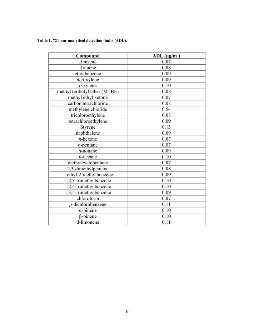
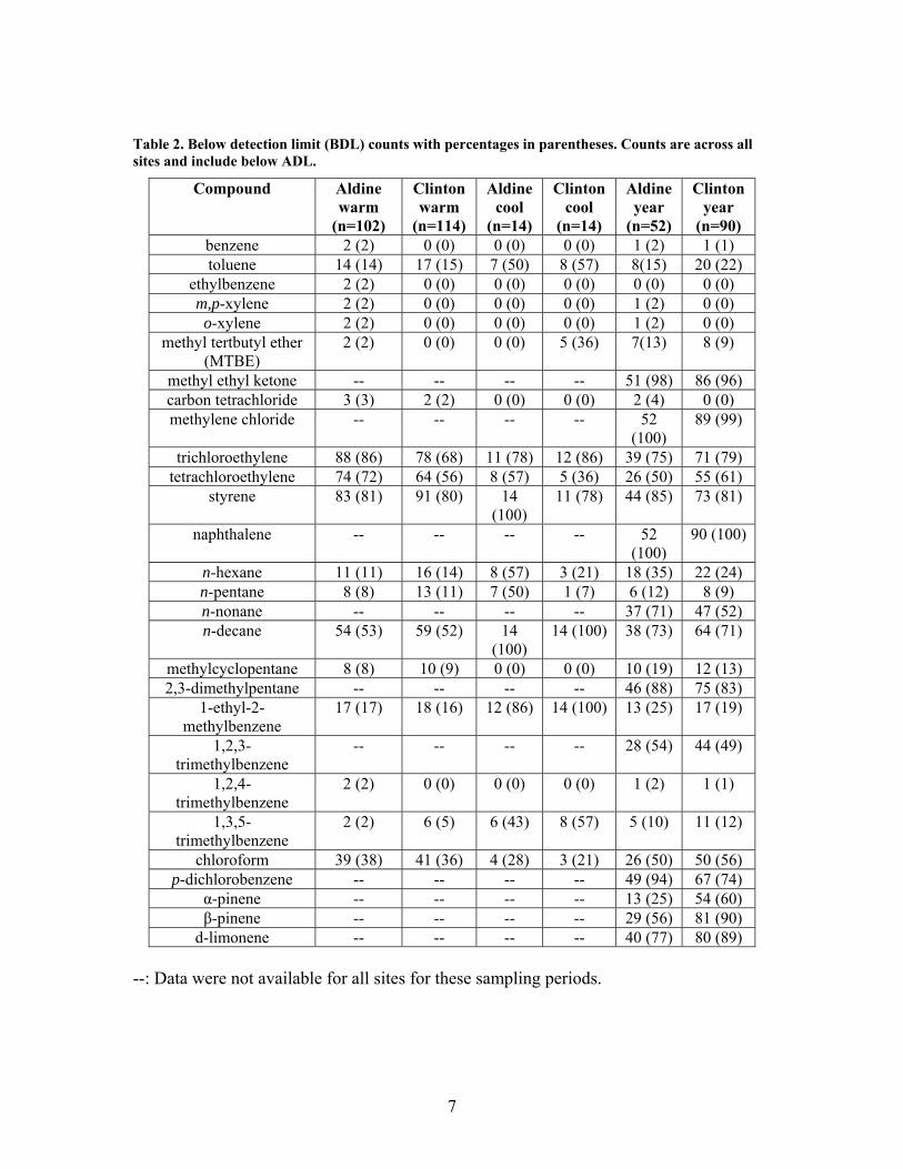
LIST OF TABLES Table 1. 72-hour analytical detection limits (ADL)............................................................ 6 Table 2. Below detection limit (BDL) counts with percentages in parentheses. Counts are
across all sites and include below ADL...................................................................... 7 Table 3. Statistically significant differences among all site groups.................................. 11 Table 4. Statistically significant differences for the pairwise comparisons. The group
with the larger concentration is indicated parenthetically. ....................................... 12 Table 5. Statistically significant time trend results for the year-long sampling at the
Aldine and Clinton centroids and TCEQ sites. Chemicals not listed did not have a statistically significant time trend at any site. ........................................................... 13
Table 6. Predominant wind directions during passive sampling periods.......................... 14 Table 7. Wind direction comparisons at the Aldine TCEQ site, A20.............................. 15 Table 8. Wind direction comparisons at the Aldine centroid site, A21............................ 16 Table 9. Wind direction comparisons at the Clinton TCEQ site, C20............................. 17 Table 10. Wind direction comparisons at the Clinton centroid site, C21. ........................ 18
iv
LIST OF FIGURES Figure 1. Greater Houston area showing the locations of monitoring sites........................ 2 Figure 2. Aldine monitoring area........................................................................................ 3 Figure 3. Clinton monitoring sites. ..................................................................................... 4 Figure 4. Aldine warm and cool weather concentrations. ................................................. 9 Figure 5. Clinton warm and cool weather concentrations. ............................................... 10
1
INTRODUCTION The spatial distribution of ambient air pollutants resulting from the influence of traffic and the potential health effects have been the subject of several studies (van Vliet et al., 1997; Roorda-Knape et al., 1998; Brauer et al., 2003). Other researchers have expanded the breadth of the factors involved by considering variables related to such things as population density and distances to point sources. This has frequently been done to attempt to predict levels of pollutants over a large geographic area; this approach has often been implemented in the form of land-use regression modeling (Jerrett et al., 2005; Smith et al., 2006).
Conventional, regulatory-based air monitoring is generally expensive and, therefore, typically conducted at only a few locations in a city. This provides limited information on intra-urban variability for air pollution. However, the development and improvements of passive sampling devices in recent years have offered the opportunity to expand sampling to a larger number of sites in a given area.
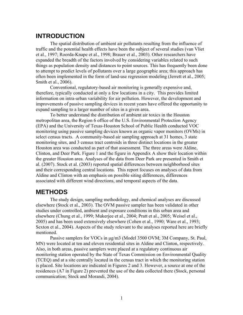
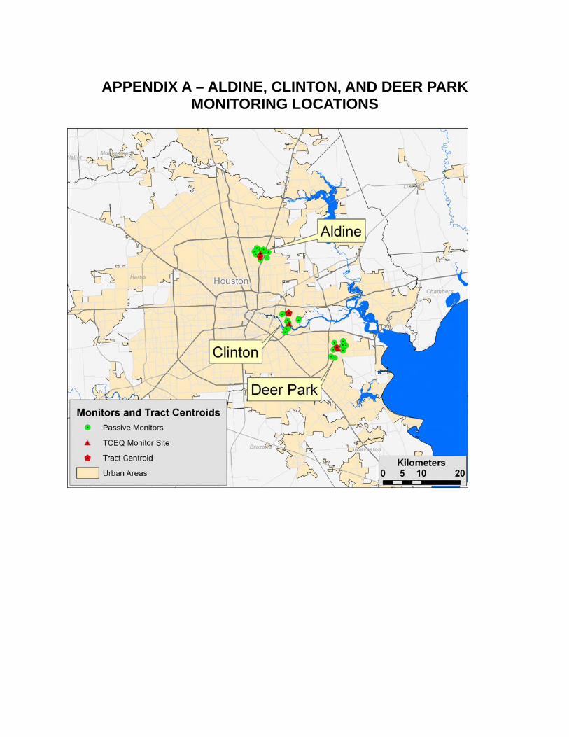
To better understand the distribution of ambient air toxics in the Houston metropolitan area, the Region 6 office of the U.S. Environmental Protection Agency (EPA) and the University of Texas-Houston School of Public Health conducted VOC monitoring using passive sampling devices known as organic vapor monitors (OVMs) in select census tracts. A community-based air sampling approach at 31 homes, 3 state monitoring sites, and 3 census tract centroids in three distinct locations in the greater Houston area was conducted as part of that assessment. The three areas were Aldine, Clinton, and Deer Park. Figure 1 and the figure in Appendix A show their location within the greater Houston area. Analyses of the data from Deer Park are presented in Smith et al. (2007). Stock et al. (2003) reported spatial differences between neighborhood sites and their corresponding central locations. This report focuses on analyses of data from Aldine and Clinton with an emphasis on possible siting differences, differences associated with different wind directions, and temporal aspects of the data.
METHODS The study design, sampling methodology, and chemical analyses are discussed
elsewhere (Stock et al., 2003). The OVM passive sampler has been validated in other studies under controlled, ambient and exposure conditions in this urban area and elsewhere (Chung et al., 1999; Mukerjee et al., 2004; Pratt et al., 2005; Weisel et al., 2005) and has been used extensively elsewhere (Cohen et al., 1990; Ware et al., 1993; Sexton et al., 2004). Aspects of the study relevant to the analyses reported here are briefly mentioned.
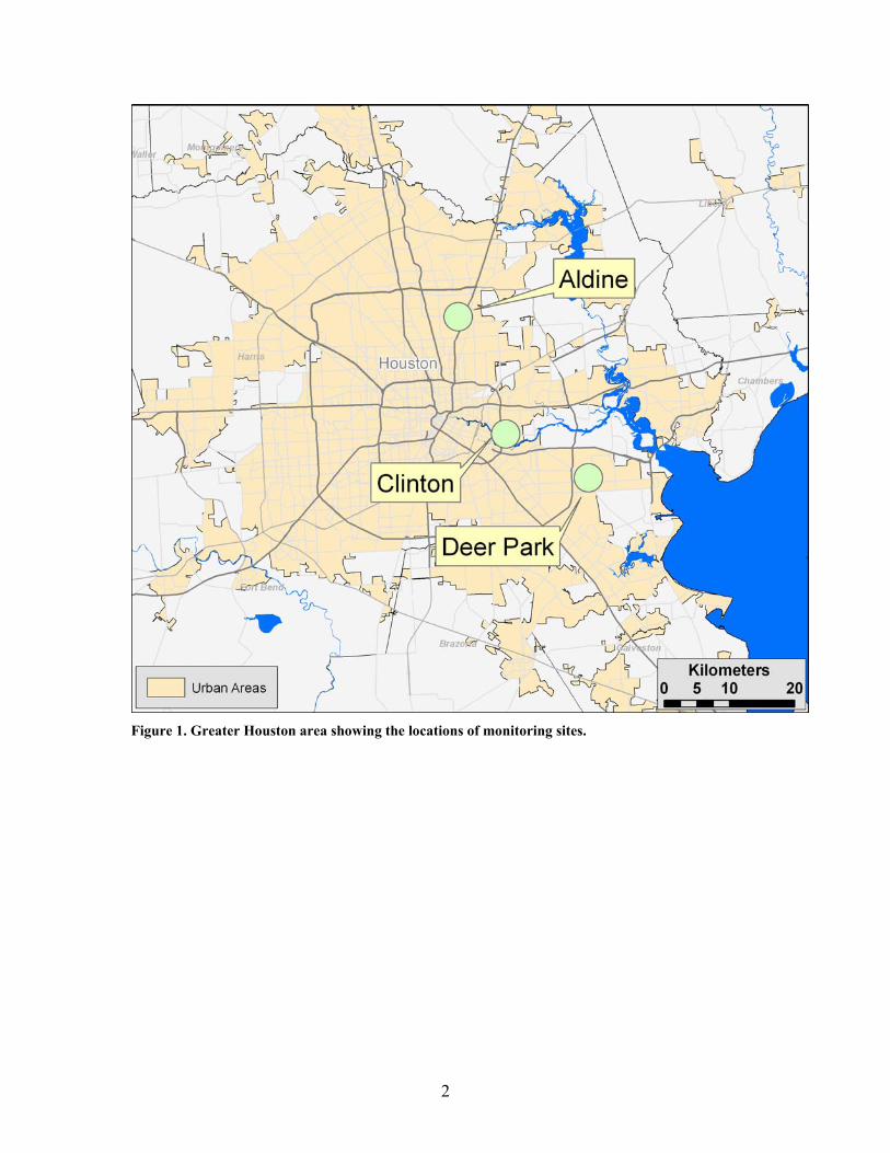
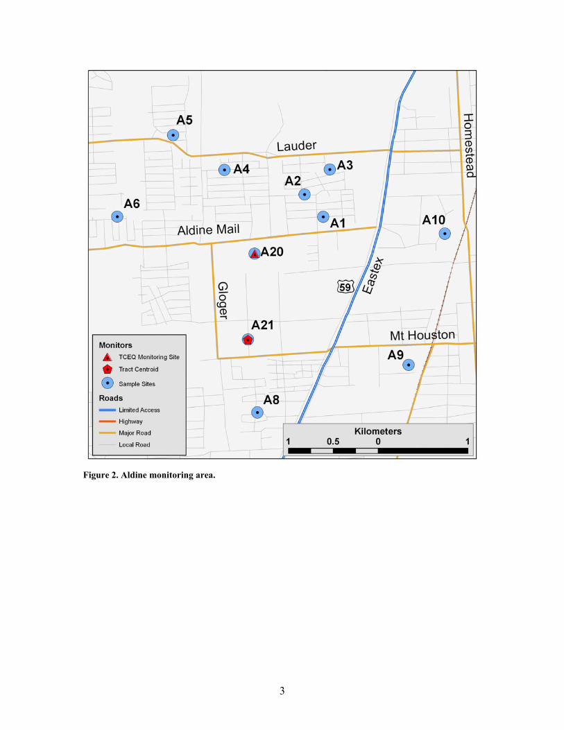
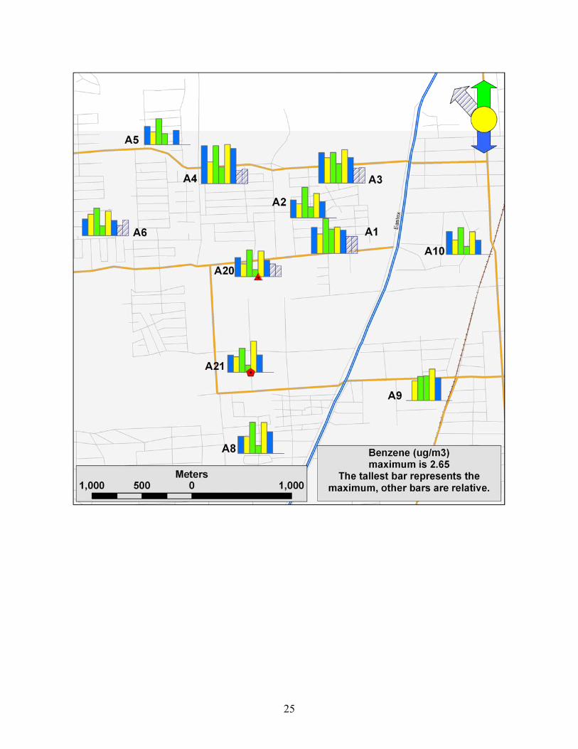
Passive samplers for VOCs in μg/m3 (Model 3500 OVM; 3M Company, St. Paul, MN) were located at ten and eleven residential sites in Aldine and Clinton, respectively. Also, in both areas, passive samplers were placed at a regulatory continuous air monitoring station operated by the State of Texas Commission on Environmental Quality (TCEQ) and at a site centrally located in the census tract in which the monitoring station is placed. Site locations are indicated in Figures 2 and 3. However, a source at one of the residences (A7 in Figure 2) prevented the use of the data collected there (Stock, personal communication; Stock and Morandi, 2004).
2
Figure 1. Greater Houston area showing the locations of monitoring sites.
3
Figure 2. Aldine monitoring area.
4
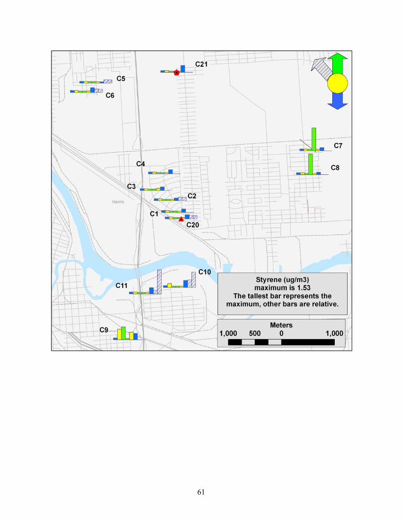
Figure 3. Clinton monitoring sites.
5
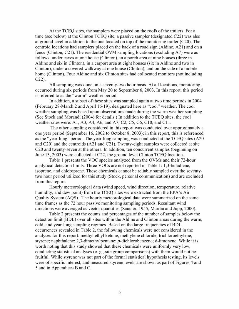
At the TCEQ sites, the samplers were placed on the roofs of the trailers. For a time (see below) at the Clinton TCEQ site, a passive sampler (designated C22) was also at ground level in addition to the one located on top of the monitoring trailer (C20). The centroid locations had samplers placed on the back of a road sign (Aldine, A21) and on a fence (Clinton, C21). The residential OVM sampling locations (excluding A7) were as follows: under eaves at one house (Clinton), in a porch area at nine houses (three in Aldine and six in Clinton), in a carport area at eight houses (six in Aldine and two in Clinton), under a covered walkway at one house (Clinton), and on the side of a mobile home (Clinton). Four Aldine and six Clinton sites had collocated monitors (not including C22).
All sampling was done on a seventy-two hour basis. At all locations, monitoring occurred during six periods from May 20 to September 6, 2003. In this report, this period is referred to as the “warm” weather period.
In addition, a subset of these sites was sampled again at two time periods in 2004 (February 28-March 2 and April 16-19), designated here as “cool” weather. The cool weather sampling was based upon observations made during the warm weather sampling. (See Stock and Morandi (2004) for details.) In addition to the TCEQ sites, the cool weather sites were: A1, A3, A4, A6, and A7; C2, C5, C6, C10, and C11.
The other sampling considered in this report was conducted over approximately a one year period (September 16, 2002 to October 8, 2003); in this report, this is referenced as the “year-long” period. The year-long sampling was conducted at the TCEQ sites (A20 and C20) and the centroids (A21 and C21). Twenty-eight samples were collected at site C20 and twenty-seven at the others. In addition, ten concurrent samples (beginning on June 13, 2003) were collected at C22, the ground level Clinton TCEQ location.
Table 1 presents the VOC species analyzed from the OVMs and their 72-hour analytical detection limits. Three VOCs are not reported in Table 1: 1,3-butadiene, isoprene, and chloroprene. These chemicals cannot be reliably sampled over the seventy-two hour period utilized for this study (Stock, personal communication) and are excluded from this report.
Hourly meteorological data (wind speed, wind direction, temperature, relative humidity, and dew point) from the TCEQ sites were extracted from the EPA’s Air Quality System (AQS). The hourly meteorological data were summarized on the same time frames as the 72 hour passive monitoring sampling periods. Resultant wind directions were averaged as vector quantities (Saucier, 1955; Mardia and Jupp, 2000).
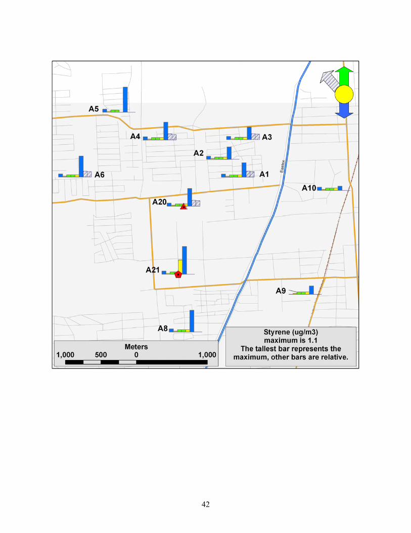
Table 2 presents the counts and percentages of the number of samples below the detection limit (BDL) over all sites within the Aldine and Clinton areas during the warm, cold, and year-long sampling regimes. Based on the large frequencies of BDL occurrences revealed in Table 2, the following chemicals were not considered in the analyses for this report: methyl ethyl ketone; methylene chloride; trichloroethylene; styrene; naphthalene; 2,3-dimethylpentane; p-dichlorobenzene; d-limonene. While it is worth noting that this study showed that these chemicals were uniformly very low, conducting statistical analyses (e. g., site group comparisons) with them would not be fruitful. While styrene was not part of the formal statistical hypothesis testing, its levels were of specific interest, and measured styrene levels are shown as part of Figures 4 and 5 and in Appendices B and C.
--: Data were not available for all sites for these sampling periods.
8
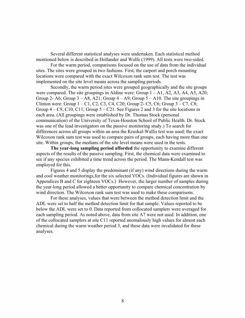
Several different statistical analyses were undertaken. Each statistical method
mentioned below is described in Hollander and Wolfe (1999). All tests were two-sided. For the warm period, comparisons focused on the use of data from the individual
sites. The sites were grouped in two fashions. First, the carport and porch mounting locations were compared with the exact Wilcoxon rank sum test. The test was implemented on the site level means across the sampling periods.
Secondly, the warm period sites were grouped geographically and the site groups were compared. The site groupings in Aldine were: Group 1 – A1, A2, A3, A4, A5, A20; Group 2- A6; Group 3 – A8, A21; Group 4 – A9; Group 5 – A10. The site groupings in Clinton were: Group 1 – C1, C2, C3, C4, C20; Group 2- C5, C6; Group 3 – C7, C8; Group 4 – C9, C10, C11; Group 5 – C21. See Figures 2 and 3 for the site locations in each area. (All groupings were established by Dr. Thomas Stock (personal communication) of the University of Texas-Houston School of Public Health. Dr. Stock was one of the lead investigators on the passive monitoring study.) To search for differences across all groups within an area the Kruskal-Wallis test was used; the exact Wilcoxon rank sum test was used to compare pairs of groups, each having more than one site. Within groups, the medians of the site level means were used in the tests.
The year-long sampling period afforded the opportunity to examine different aspects of the results of the passive sampling. First, the chemical data were examined to see if any species exhibited a time trend across the period. The Mann-Kendall test was employed for this.
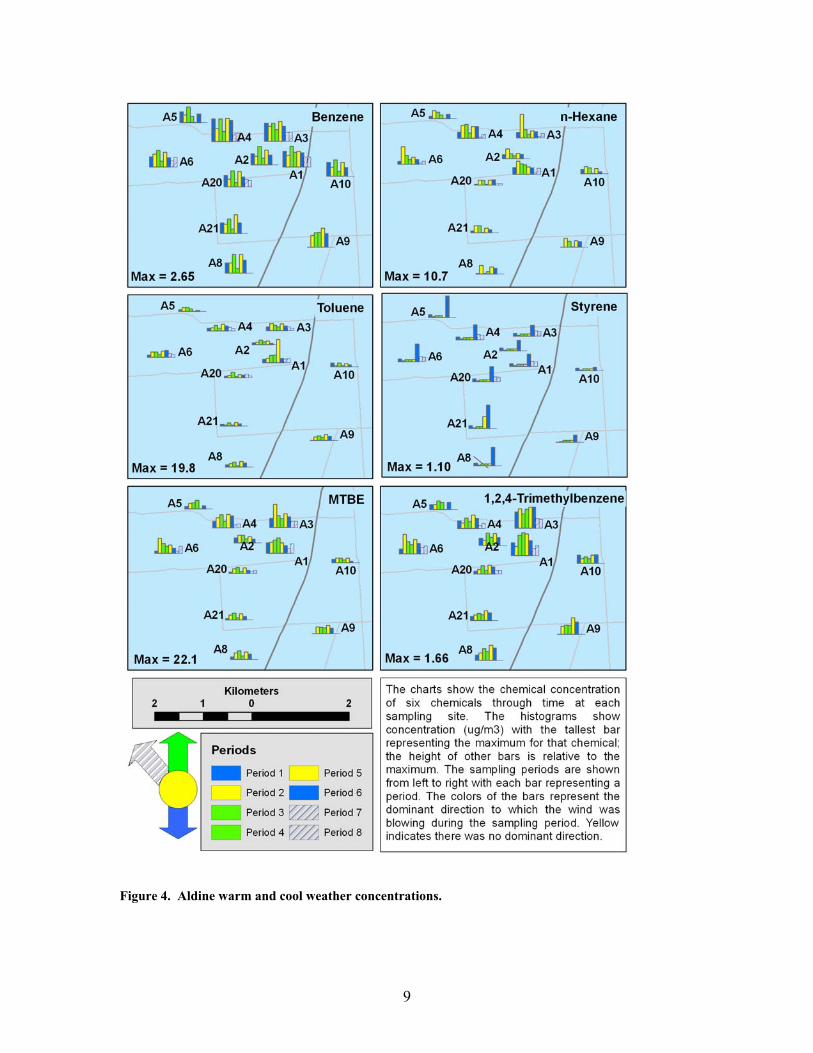
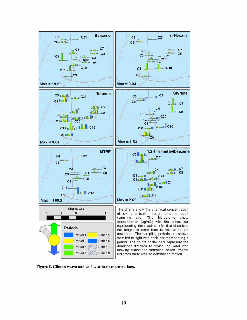
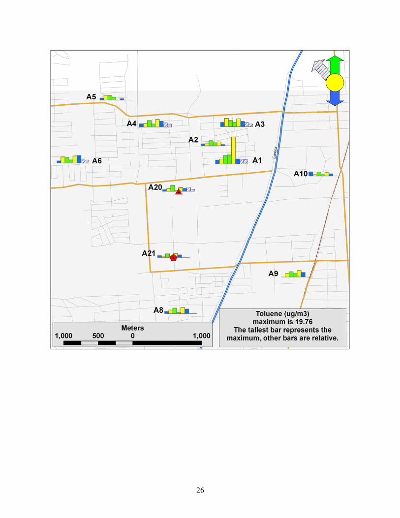
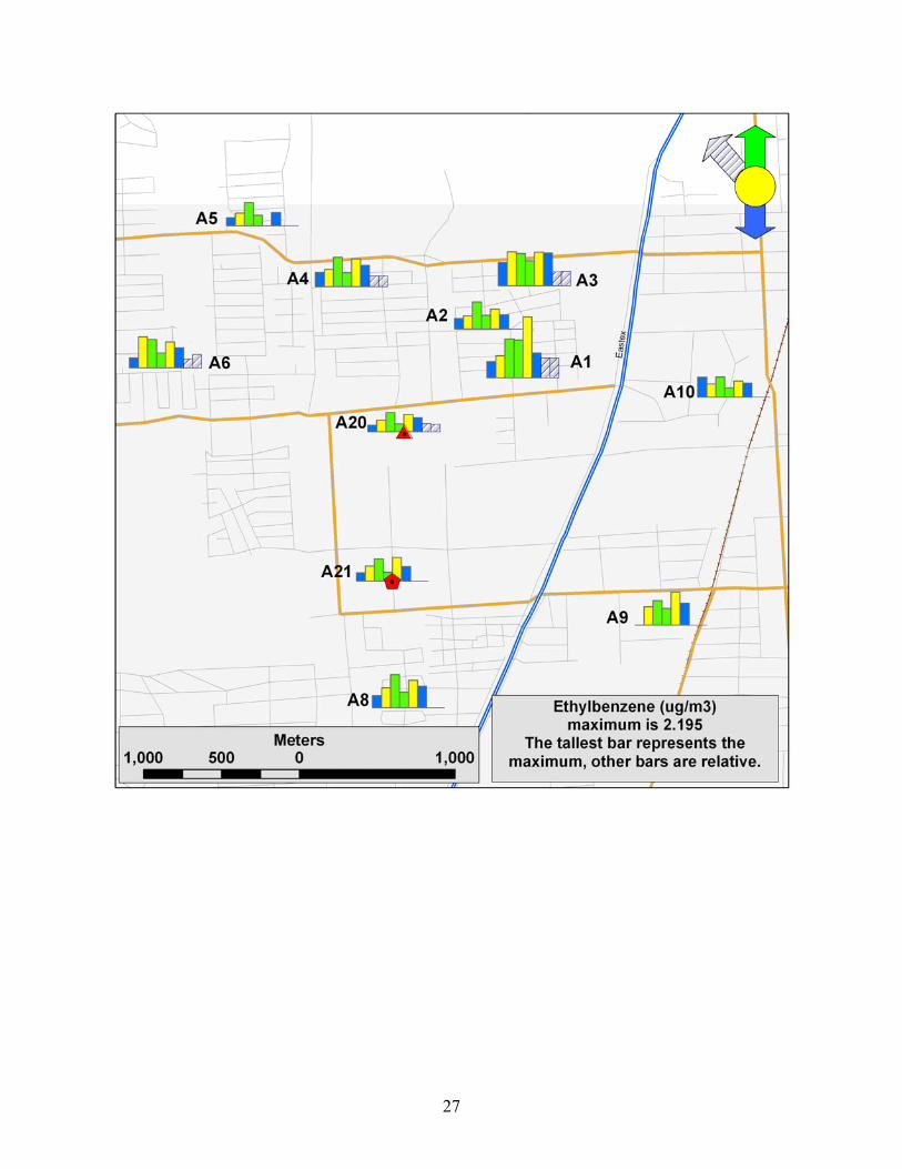
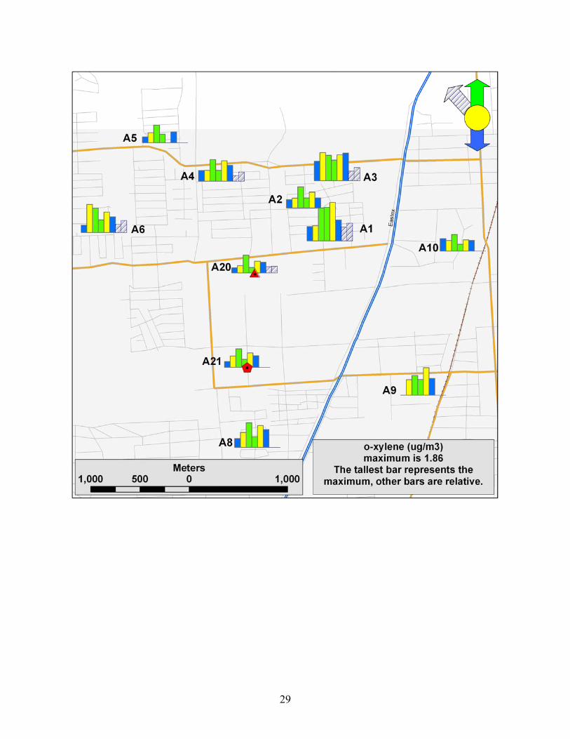
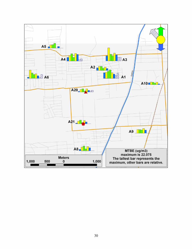
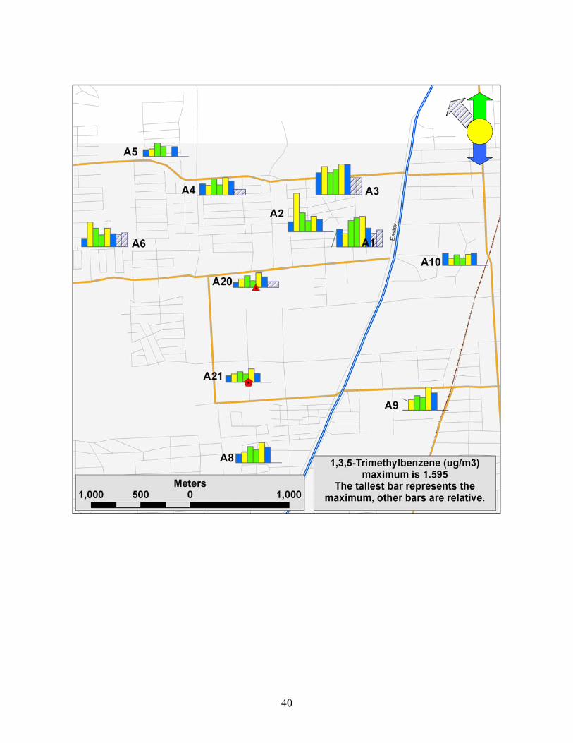
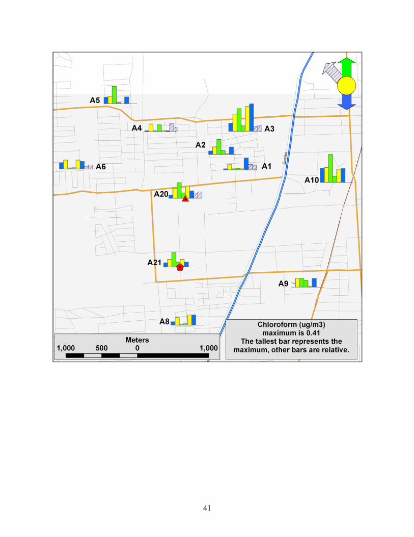
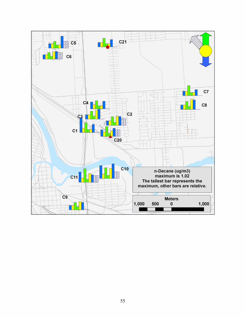
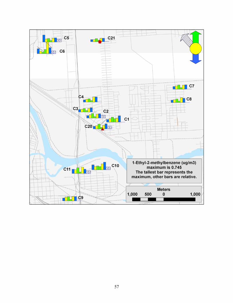
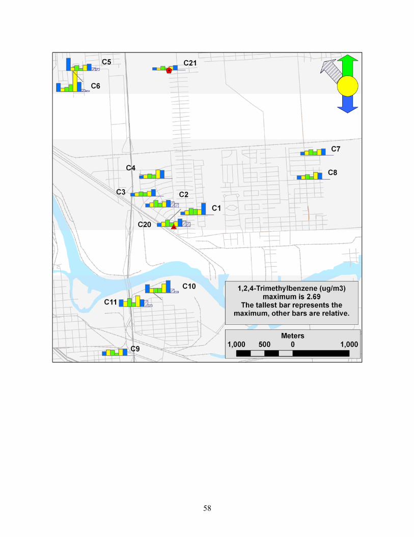
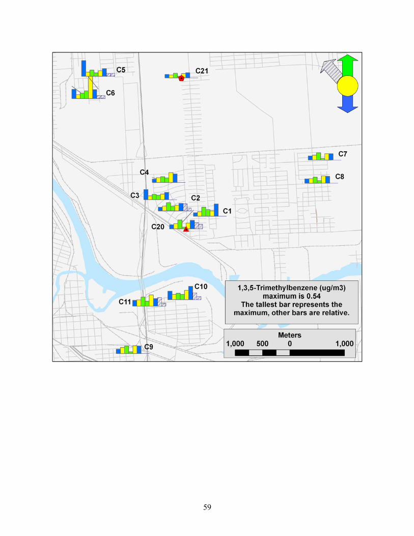
Figures 4 and 5 display the predominant (if any) wind directions during the warm and cool weather monitorings,for the six selected VOCs. (Individual figures are shown in Appendices B and C for eighteen VOCs.) However, the larger number of samples during the year-long period allowed a better opportunity to compare chemical concentration by wind direction. The Wilcoxon rank sum test was used to make these comparisons.
For these analyses, values that were between the method detection limit and the ADL were set to half the method detection limit for that sample. Values reported to be below the ADL were set to 0. Data reported from collocated samplers were averaged for each sampling period. As noted above, data from site A7 were not used. In addition, one of the collocated samplers at site C11 reported anomalously high values for almost each chemical during the warm weather period 3, and these data were invalidated for these analyses.
9
Figure 4. Aldine warm and cool weather concentrations.
10
Figure 5. Clinton warm and cool weather concentrations.
11
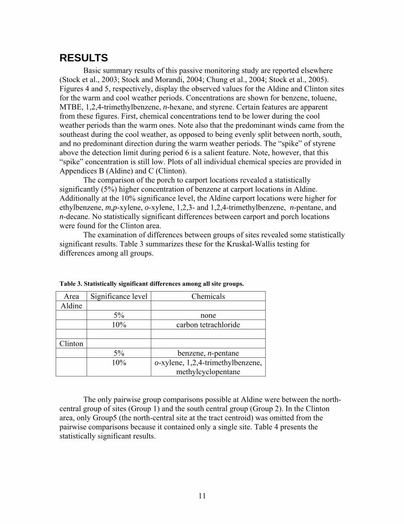
RESULTS Basic summary results of this passive monitoring study are reported elsewhere
(Stock et al., 2003; Stock and Morandi, 2004; Chung et al., 2004; Stock et al., 2005). Figures 4 and 5, respectively, display the observed values for the Aldine and Clinton sites for the warm and cool weather periods. Concentrations are shown for benzene, toluene, MTBE, 1,2,4-trimethylbenzene, n-hexane, and styrene. Certain features are apparent from these figures. First, chemical concentrations tend to be lower during the cool weather periods than the warm ones. Note also that the predominant winds came from the southeast during the cool weather, as opposed to being evenly split between north, south, and no predominant direction during the warm weather periods. The “spike” of styrene above the detection limit during period 6 is a salient feature. Note, however, that this “spike” concentration is still low. Plots of all individual chemical species are provided in Appendices B (Aldine) and C (Clinton).
The comparison of the porch to carport locations revealed a statistically significantly (5%) higher concentration of benzene at carport locations in Aldine. Additionally at the 10% significance level, the Aldine carport locations were higher for ethylbenzene, m,p-xylene, o-xylene, 1,2,3- and 1,2,4-trimethylbenzene, n-pentane, and n-decane. No statistically significant differences between carport and porch locations were found for the Clinton area.
The examination of differences between groups of sites revealed some statistically significant results. Table 3 summarizes these for the Kruskal-Wallis testing for differences among all groups.
Table 3. Statistically significant differences among all site groups.
Area Significance level Chemicals Aldine
5% none 10% carbon tetrachloride
Clinton 5% benzene, n-pentane 10% o-xylene, 1,2,4-trimethylbenzene,
methylcyclopentane
The only pairwise group comparisons possible at Aldine were between the north-
central group of sites (Group 1) and the south central group (Group 2). In the Clinton area, only Group5 (the north-central site at the tract centroid) was omitted from the pairwise comparisons because it contained only a single site. Table 4 presents the statistically significant results.
12
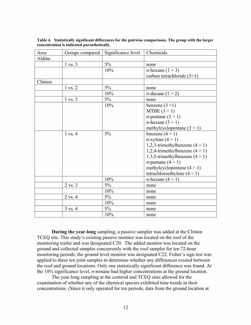
Table 4. Statistically significant differences for the pairwise comparisons. The group with the larger concentration is indicated parenthetically.
Area Groups compared Significance level Chemicals Aldine 1 vs. 3 5% none 10% n-hexane (1 > 3)
carbon tetrachloride (3>1) Clinton 1 vs. 2 5% none 10% n-decane (1 > 2) 1 vs. 3 5% none 10% benzene (3 >1)
10% n-hexane (4 > 1) 2 vs. 3 5% none 10% none 2 vs. 4 5% none 10% none 3 vs. 4 5% none 10% none
During the year-long sampling, a passive sampler was added at the Clinton
TCEQ site. This study’s existing passive monitor was located on the roof of the monitoring trailer and was designated C20. The added monitor was located on the ground and collected samples concurrently with the roof sampler for ten 72-hour monitoring periods; the ground level monitor was designated C22. Fisher’s sign test was applied to these ten joint samples to determine whether any differences existed between the roof and ground locations. Only one statistically significant difference was found. At the 10% significance level, n-nonane had higher concentrations at the ground location.
The year-long sampling at the centroid and TCEQ sites allowed for the examination of whether any of the chemical species exhibited time trends in their concentrations. (Since it only operated for ten periods, data from the ground location at
13
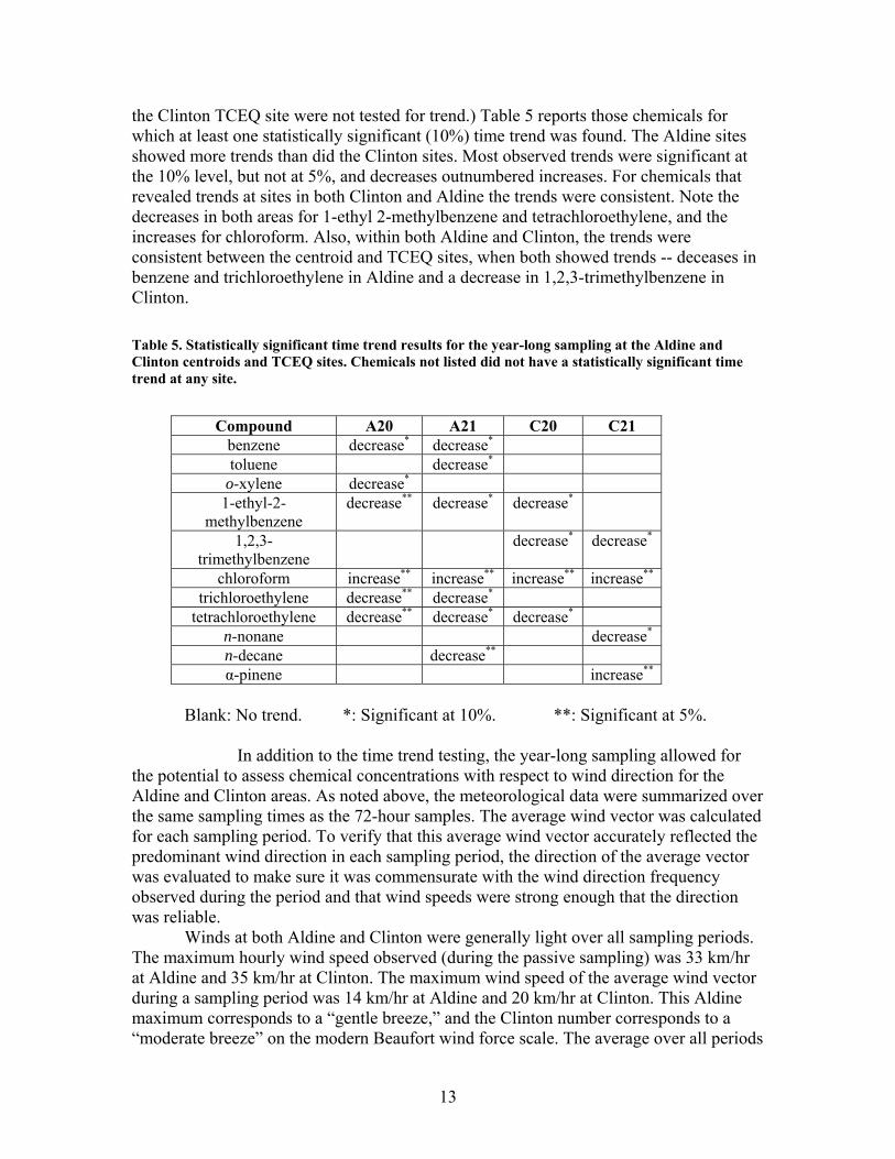
the Clinton TCEQ site were not tested for trend.) Table 5 reports those chemicals for which at least one statistically significant (10%) time trend was found. The Aldine sites showed more trends than did the Clinton sites. Most observed trends were significant at the 10% level, but not at 5%, and decreases outnumbered increases. For chemicals that revealed trends at sites in both Clinton and Aldine the trends were consistent. Note the decreases in both areas for 1-ethyl 2-methylbenzene and tetrachloroethylene, and the increases for chloroform. Also, within both Aldine and Clinton, the trends were consistent between the centroid and TCEQ sites, when both showed trends -- deceases in benzene and trichloroethylene in Aldine and a decrease in 1,2,3-trimethylbenzene in Clinton.
Table 5. Statistically significant time trend results for the year-long sampling at the Aldine and Clinton centroids and TCEQ sites. Chemicals not listed did not have a statistically significant time trend at any site.
Blank: No trend. *: Significant at 10%. **: Significant at 5%. In addition to the time trend testing, the year-long sampling allowed for
the potential to assess chemical concentrations with respect to wind direction for the Aldine and Clinton areas. As noted above, the meteorological data were summarized over the same sampling times as the 72-hour samples. The average wind vector was calculated for each sampling period. To verify that this average wind vector accurately reflected the predominant wind direction in each sampling period, the direction of the average vector was evaluated to make sure it was commensurate with the wind direction frequency observed during the period and that wind speeds were strong enough that the direction was reliable.
Winds at both Aldine and Clinton were generally light over all sampling periods. The maximum hourly wind speed observed (during the passive sampling) was 33 km/hr at Aldine and 35 km/hr at Clinton. The maximum wind speed of the average wind vector during a sampling period was 14 km/hr at Aldine and 20 km/hr at Clinton. This Aldine maximum corresponds to a “gentle breeze,” and the Clinton number corresponds to a “moderate breeze” on the modern Beaufort wind force scale. The average over all periods
14
was 7 km/hr at Aldine and 4 km/hr at Clinton; on the Beaufort scale, these values correspond to a “light breeze” and “light air,” respectively.
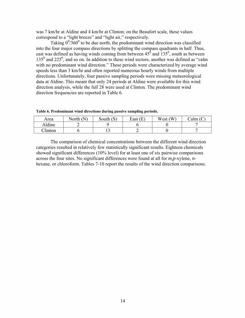
Taking 00/3600 to be due north, the predominant wind direction was classified into the four major compass directions by splitting the compass quadrants in half. Thus, east was defined as having winds coming from between 450 and 1350, south as between 1350 and 2250, and so on. In addition to these wind sectors, another was defined as “calm with no predominant wind direction.” These periods were characterized by average wind speeds less than 3 km/hr and often reported numerous hourly winds from multiple directions. Unfortunately, four passive sampling periods were missing meteorological data at Aldine. This meant that only 24 periods at Aldine were available for this wind direction analysis, while the full 28 were used at Clinton. The predominant wind direction frequencies are reported in Table 6.
Table 6. Predominant wind directions during passive sampling periods.
Area North (N) South (S) East (E) West (W) Calm (C) Aldine 2 9 6 0 7 Clinton 6 13 2 0 7
The comparison of chemical concentrations between the different wind direction
categories resulted in relatively few statistically significant results. Eighteen chemicals showed significant differences (10% level) for at least one of six pairwise comparisons across the four sites. No significant differences were found at all for m,p-xylene, n-hexane, or chloroform. Tables 7-10 report the results of the wind direction comparisons.
15
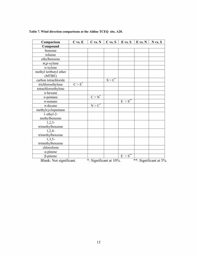
Table 7. Wind direction comparisons at the Aldine TCEQ site, A20.
Comparison C vs. E C vs. N C vs. S E vs. S E vs. N N vs. S Compound
benzene toluene
ethylbenzene m,p-xylene o-xylene
methyl tertbutyl ether (MTBE)
carbon tetrachloride S > C* trichloroethylene C > E*
tetrachloroethylene n-hexane n-pentane C > N* n-nonane E > S** n-decane N > C*
methylcyclopentane 1-ethyl-2-
methylbenzene
1,2,3-trimethylbenzene
1,2,4-trimethylbenzene
1,3,5-trimethylbenzene
chloroform α-pinene β-pinene E > S**
Blank: Not significant. *: Significant at 10%. **: Significant at 5%.
16
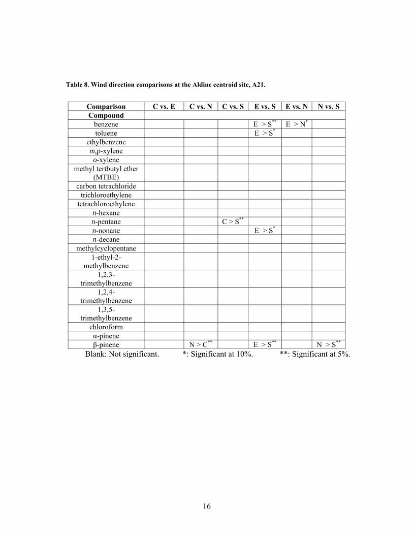
Table 8. Wind direction comparisons at the Aldine centroid site, A21.
Comparison C vs. E C vs. N C vs. S E vs. S E vs. N N vs. S Compound
benzene E > S** E > N* toluene E > S*
ethylbenzene m,p-xylene o-xylene
methyl tertbutyl ether (MTBE)
carbon tetrachloride trichloroethylene
tetrachloroethylene n-hexane n-pentane C > S** n-nonane E > S* n-decane
methylcyclopentane 1-ethyl-2-
methylbenzene
1,2,3-trimethylbenzene
1,2,4-trimethylbenzene
1,3,5-trimethylbenzene
chloroform α-pinene β-pinene N > C** E > S** N > S**
Blank: Not significant. *: Significant at 10%. **: Significant at 5%.
17
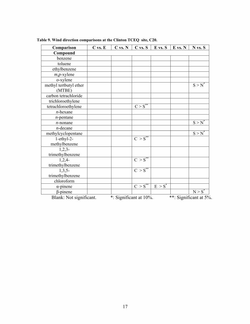
Table 9. Wind direction comparisons at the Clinton TCEQ site, C20.
Comparison C vs. E C vs. N C vs. S E vs. S E vs. N N vs. S Compound
benzene toluene
ethylbenzene m,p-xylene o-xylene
methyl tertbutyl ether (MTBE)
S > N*
carbon tetrachloride trichloroethylene
tetrachloroethylene C > S** n-hexane n-pentane n-nonane S > N* n-decane
methylcyclopentane S > N* 1-ethyl-2-
methylbenzene C > S**
1,2,3-trimethylbenzene
1,2,4-trimethylbenzene
C > S**
1,3,5-trimethylbenzene
C > S**
chloroform α-pinene C > S** E > S* β-pinene N > S*
Blank: Not significant. *: Significant at 10%. **: Significant at 5%.
18
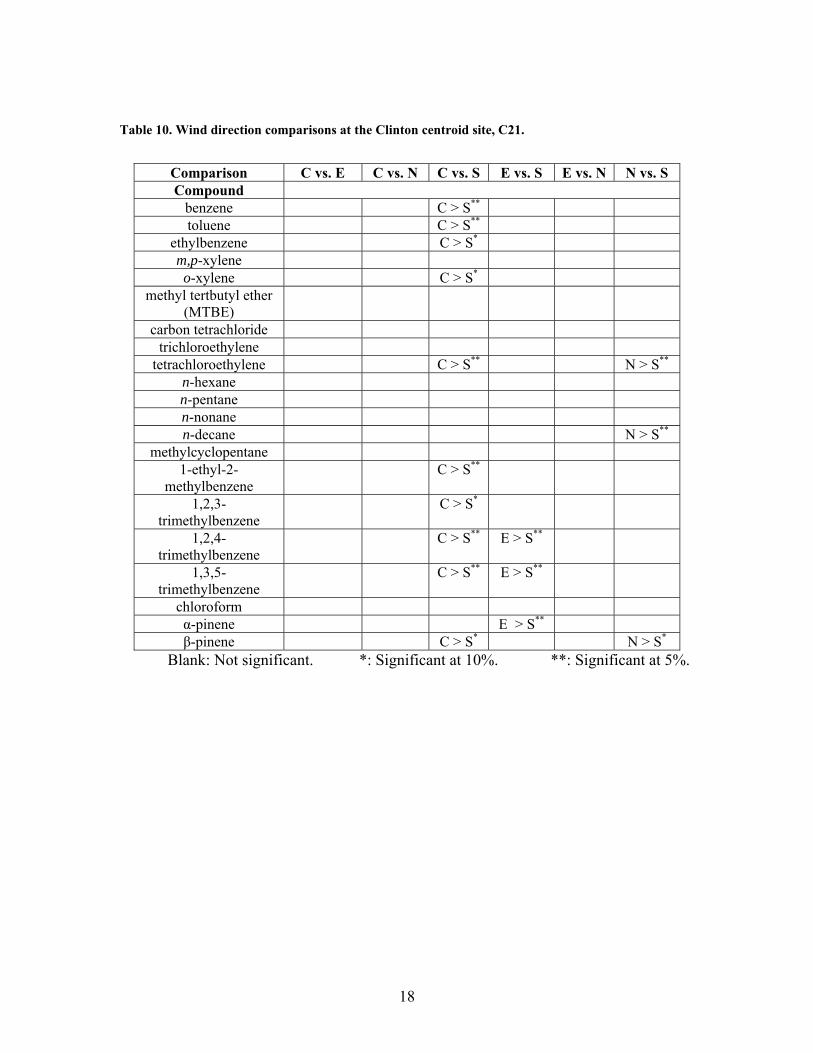
Table 10. Wind direction comparisons at the Clinton centroid site, C21.
Comparison C vs. E C vs. N C vs. S E vs. S E vs. N N vs. S Compound
benzene C > S** toluene C > S**
ethylbenzene C > S* m,p-xylene o-xylene C > S*
methyl tertbutyl ether (MTBE)
carbon tetrachloride trichloroethylene
tetrachloroethylene C > S** N > S** n-hexane n-pentane n-nonane n-decane N > S**
methylcyclopentane 1-ethyl-2-
methylbenzene C > S**
1,2,3-trimethylbenzene
C > S*
1,2,4-trimethylbenzene
C > S** E > S**
1,3,5-trimethylbenzene
C > S** E > S**
chloroform α-pinene E > S** β-pinene C > S* N > S*
Blank: Not significant. *: Significant at 10%. **: Significant at 5%.
19
SUMMARY This analysis of the data from these monitoring efforts in the Aldine and Clinton
areas has led to the following general results. Chemical concentrations appear to be lower during the relatively cool months of
the year than during the summertime. It would be interesting to see if this result were also obtained during other years than those examined here and with a longer period of monitoring during the cooler weather.
The comparison of the carport to the porch locations suggested that gasoline related species were higher in the carport locations. This result is not too surprising, given that vehicles generate some emissions in carports. Though no statistically significant difference was found in this respect for the Clinton sites, it should be recalled that there were only two carport locations in Clinton and consequently the statistical test’s power was limited in this case.
The overall comparison of the site groupings with the Kruskal-Wallis test gave virtually no indication of differences at Aldine. (Only carbon tetrachloride was statistically different, and this was at the 10% level.) The Clinton groupings did reveal some differences. Across all groupings, the differences were primarily in gasoline related compounds (benzene, n-pentane, o-xylene, and 1,2,4-trimethylbenzene), but also methylcyclopentane.
Following the comparisons using all groupings, the more focused pairwise comparisons with the Wilcoxon rank sum test mimicked these results. Very little difference was found at Aldine. However, the tests at Clinton detected several differences between Group 1 (central group) and Groups 3 (to the east) and 4 (south of the ship channel, in the Manchester area). Group 1 was found to have lower concentrations than either Group 3 or Group 4. Generally, these differences were for gasoline related compounds (benzene, o-xylene, the trimethylbenzenes, n-pentane, n-hexane, and MTBE) though not exclusively so, as methylcyclopentane and tetrachloroethylene were also lower in Group 1. By the way, it is interesting to note that Group 1 contains the Clinton TCEQ site.
The ground and roof locations at the Clinton TCEQ site showed no salient differences.
Though the testing for time trends over the year-long sampling did find a few statistically significant trends at the TCEQ and centroid sites, these were few and far between. Most compounds had no trend. Of the cases where trends were found, the Aldine sites showed more trends than did the Clinton sites. Most observed trends were significant at the 10% level, but not at 5%, and decreases outnumbered increases. For chemicals that revealed trends at sites in both Clinton and Aldine the trends were consistent -- decreases in both areas for 1-ethyl 2-methylbenzene and tetrachloroethylene and increases for chloroform. Also, within both Aldine and Clinton, the trends were consistent between the centroid and TCEQ sites, when both showed trends -- deceases in benzene and trichloroethylene in Aldine and a decrease in 1,2,3-trimethylbenzene in Clinton.
Finally, testing for chemical concentration differences based on wind direction uncovered some differences at the Clinton sites but very few at either of the Aldine
20
locations. When differences were found at the Clinton centroid site (C21), concentrations were lower with southerly winds, as opposed to easterly, northerly, or periods with no predominant wind direction. Again differences were found primarily for gasoline related compounds, though not only these. At the Clinton TCEQ site (C20), concentration differences were usually manifested as lower levels for southerly winds versus conditions with no predominant direction. In contrast, however, this site also showed higher concentrations with southerly winds versus northerly winds for MTBE, n-nonane, and methylcyclopentane.
REFERENCES Brauer M., Hoek G., van Vliet P., Meliefste K., Fischer P., Gehring U., Heinrich J., Cyrys J., Bellander T., Lewne M, and Brunekreef B. 2003. Estimating long-term average particulate air pollution concentrations: application of traffic indicators and geographic information systems. Epidemiol. 14: 228-239. Chung, C.W., Morandi, M.T., Stock, T.H., and Afshar, M. 1999. Evaluation of a passive sampler for volatile organic compounds at ppb concentrations, varying temperatures, and humidities with 24-hr Exposures. 2. Sampler Performance. Environ. Sci. Technol. 33: 3666-3671. Chung, K.C., Stock, T.H., Morandi, M.T., and Afshar, M. 2004. Evaluation and use of diffusive air samplers for determining temporal and spatial variation of volatile organic compounds in the ambient air of urban communities. in Proceedings of the 97th Annual Conference of the Air & Waste Management Association, Indianapolis, IN. Cohen, M.A., Ryan, P.B., Yanagisawa, Y., Spengler, J.D., Özkaynak, H., and Epstein, P.S. 1990. The validation of a passive sampler for indoor and outdoor concentrations of volatile organic compounds. J. Air &Waste Manage. Assoc. 40: 993-997. Graedel T.E., 1978. Chemical Compounds in the Atmosphere, Academic Press, New York, 440 pp. Hollander, M. and Wolfe, D.A. 1999. Nonparametric Statistical Methods, Wiley, New York, 787 pp. Jerrett, M., Arain, A., Kanaroglou, P., Beckerman, B., Potoglou, D., Sahsuvaroglu, T., Morrison J., and Giovis, C., 2005. A review and evaluation of intraurban air pollution exposure models. J. Exp. Anal. Environ. Epidemiol. 15: 185-204. Mardia, K.V. and Jupp, P.E. 2000. Directional Statistics, John Wiley and Sons, Chichester, England, 429 pp.
21
Mukerjee, S., Smith, L.A., Norris, G.A., Morandi, M.T., Gonzales, M., Noble, C.A., Neas, L.M., and Özkaynak, A.H. 2004. Field method comparison between passive air samplers and continuous monitors for volatile organic compounds and NO2 in El Paso, Texas, USA. J. Air &Waste Manage. Assoc. 54: 307-319. Pratt G.C., Bock D., Stock T.H., Morandi, M., Adgate J.L., Ramachandran G., Mongin S.J., and Sexton K. 2005. A field comparison of volatile organic compound measurements using passive organic vapor monitors and stainless steel canisters. Environ. Sci. Technol. 39: 3261-3268. Roorda-Knape M.C., Janssen N.A.H., de Hartog J.J., van Vliet P.H.N., Harssema H., and Brunekreef B. 1998. Air pollution from traffic in city districts near major motorways. Atmos. Environ. 32: 1921-1930. Saucier, W.J., 1955, Principles of Meteorological Analysis, University of Chicago Press, Chicago, 438 pp. Sexton K, Adgate JL, Mongin SJ , Pratt GC, Ramachandran G, Stock TH , and Morandi M. 2004. Evaluating differences between measured personal exposures to volatile organic compounds and concentrations in outdoor and indoor air. Environ. Sci. Technol. 38: 2593-2602. Smith, L., Mukerjee, S., Gonzales, M., Stallings, C., Neas, L., Norris, G. and Özkaynak, H. 2006. Use of GIS and ancillary variables to predict volatile organic compound and nitrogen dioxide levels at unmonitored locations. Atmos. Environ. 40:3773-3787. Smith, L. A., Stock, T. H., Chung, K. C., Mukerjee, S., Liao, X. L., Stallings, C., and Ashfar, M. 2007. Spatial analysis of volatile organic compounds from a community-based air toxics monitoring network in Deer Park, Texas, USA. Environ. Monit. Assess. 128:369-379. Stock, T. H., M. T. Morandi, and M. Afshar. 2003. Ambient Air Toxics in the Houston-Galveston Area with High and Low TRI Emissions – A Pilot Study of Temporal and Spatial Concentrations Using Passive Sampling Devices (PSDs). Final Report for Tasks 2 and 3. Report to US EPA Region 6, December 2003. Stock, T. H., and M. T. Morandi. 2004. Ambient Air Toxics in the Houston-Galveston Area with High and Low TRI Emissions – A Pilot Study of Temporal and Spatial Concentrations Using Passive Sampling Devices (PSDs). Final Report for Task 3 Supplementary Monitoring Project. Report to US EPA Region 6, October 2004. Stock, T. H., M. T. Morandi, M. Afshar, and Chung, K. C. 2005. Temporal and spatial variation of air toxics in census tracts with high or low density of TRI emissions using passive sampling. in Proceedings of the 98th Annual Conference of the Air & Waste Management Association, Minneapolis, MN.
22
van Vliet P., Knape M., de Hartog J., Janssen N., Harssema H., and Brunekreef B. 1997. Motor vehicle exhaust and chronic respiratory symptoms in children living near freeways. Environ. Res. 74: 122-132. Ware, J.H., Spengler, J.D., Neas, L.M., Samet, J.M., Wagner, G.R., Coultas, D., Özkaynak, H., and Schwab, M. 1993. Respiratory and irritant health effects of ambient volatile organic compounds: the Kanawha County Health Study. Amer. J. Epidemiol. 137: 1287-1301. Weisel, C.P., Zhang J., Turpin B.J., Morandi M.T., Colome S., Stock T.H., Spektor D.M., Korn L., Winer A., Alimokhtari S.Kwon J., Mohan K., Harrington R., Giovanetti R., Cui W., Afshar M., Maberti S., and Shendell D. 2005. Relationship of Indoor, Outdoor and Personal Air (RIOPA) study: study design, methods and quality assurance/control results. J. Expos. Anal. Environ. Epidemiol. 15, 123-137.
APPENDIX A – ALDINE, CLINTON, AND DEER PARK MONITORING LOCATIONS
24
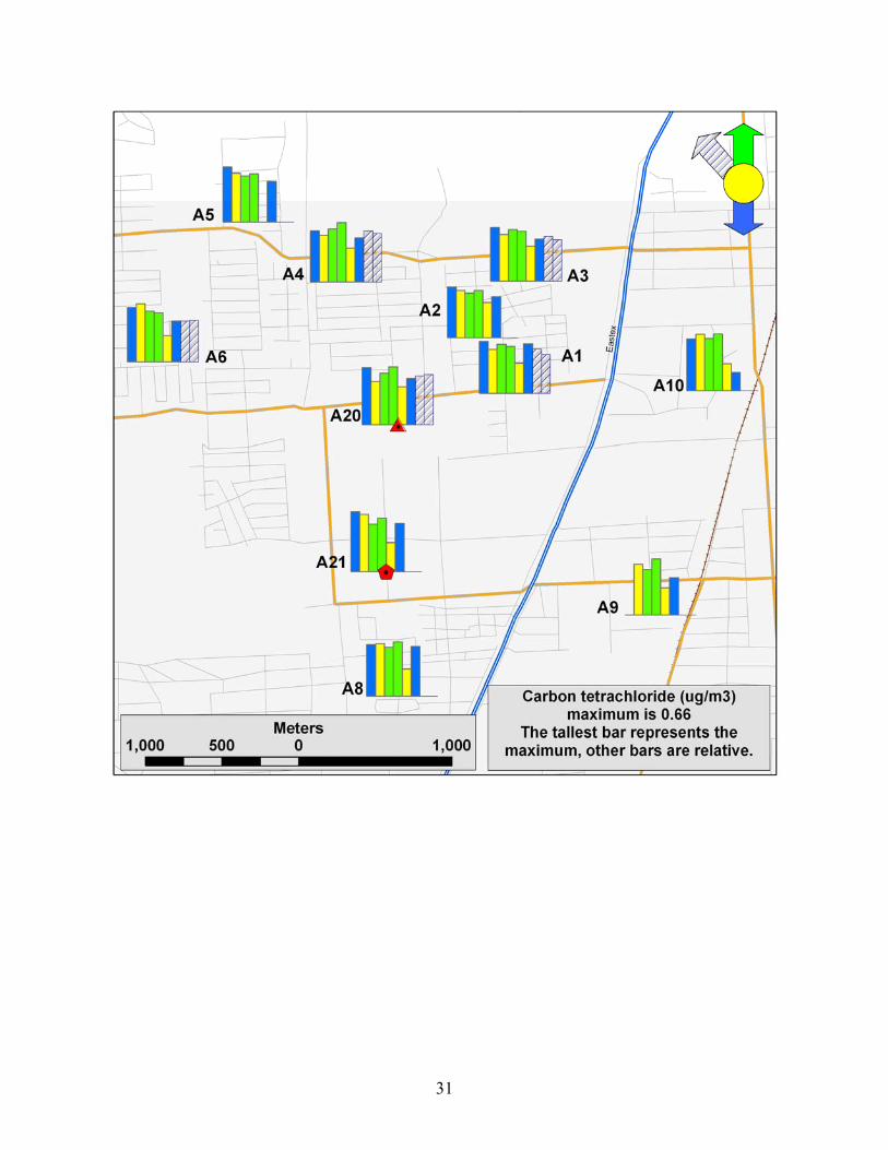
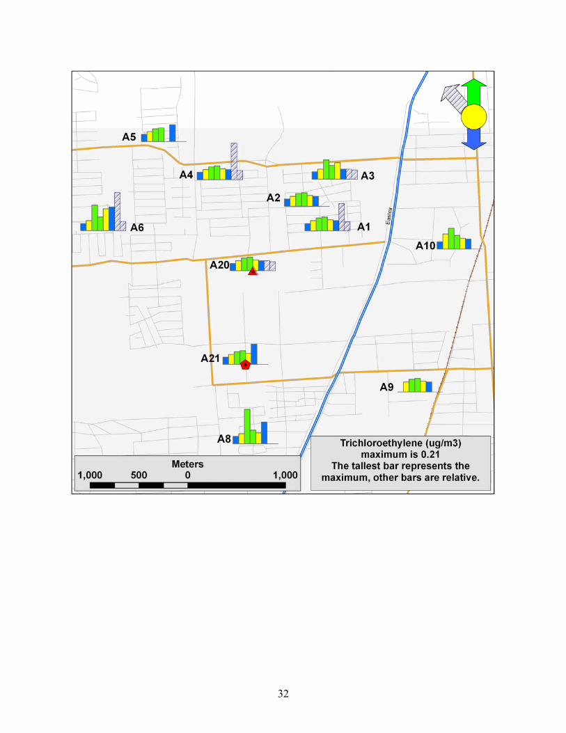
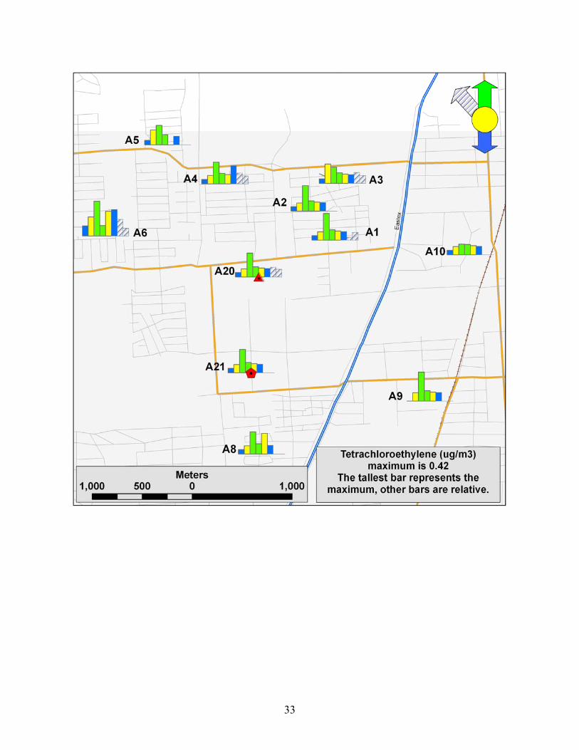
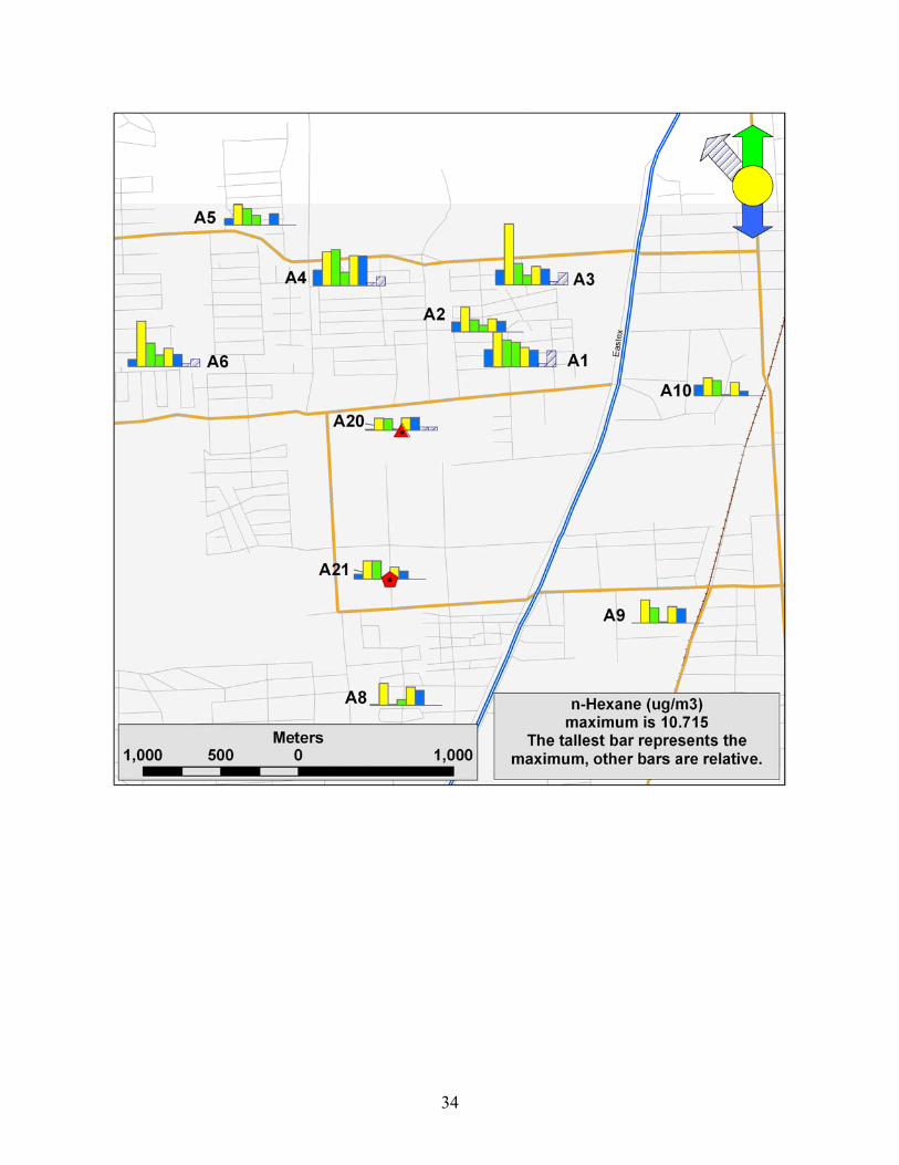
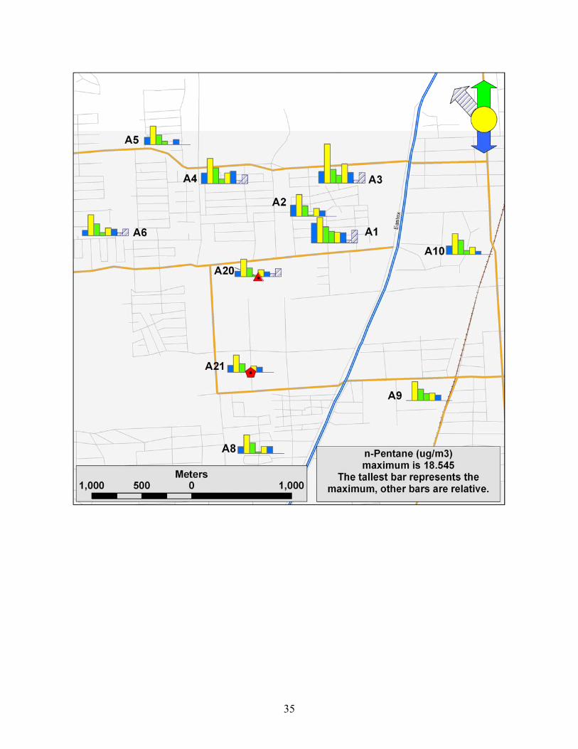
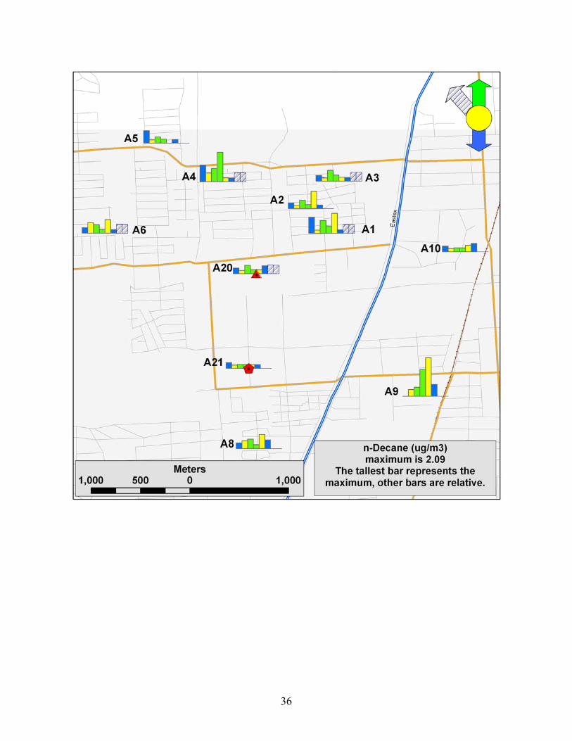
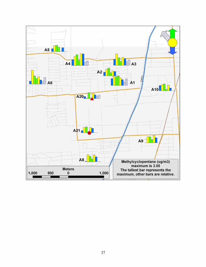
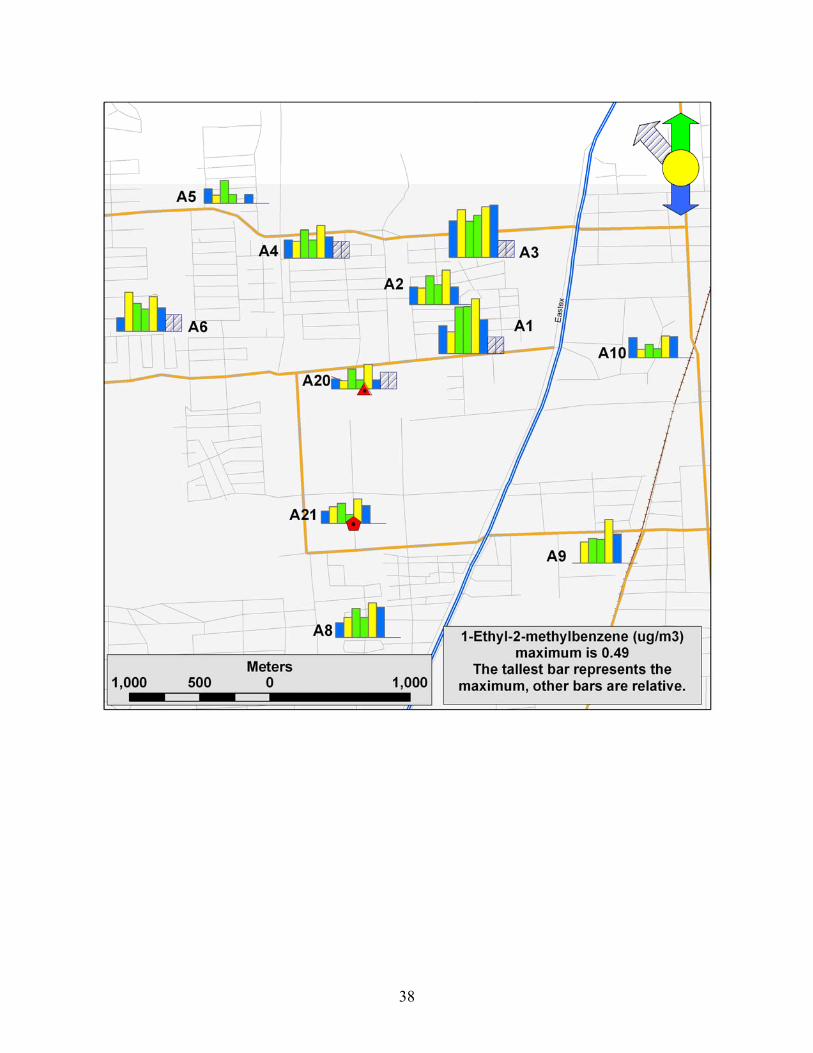
APPENDIX B – WARM AND COOL WEATHER CONCENTRATIONS FOR INDIVIDUAL CHEMICALS AT THE
ALDINE SITES
25
26
27
28
29
30
31
32
33
34
35
36
37
38
39
40
41
42
43
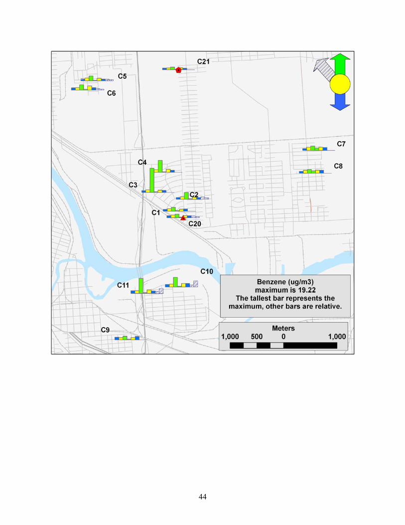
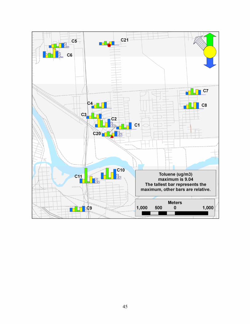
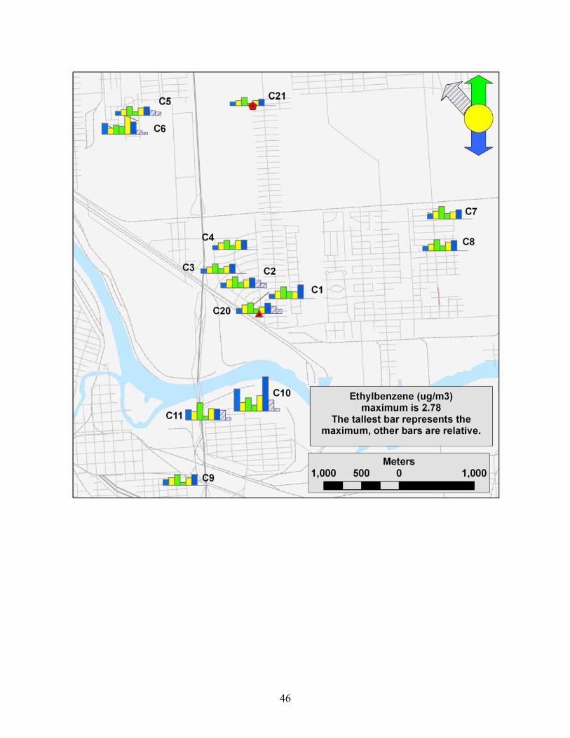
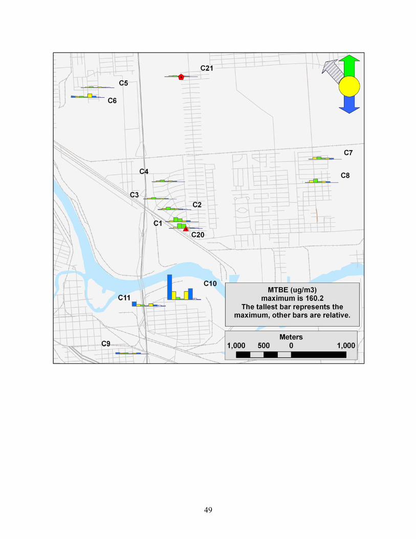
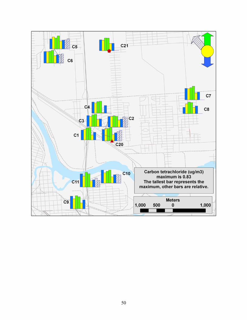
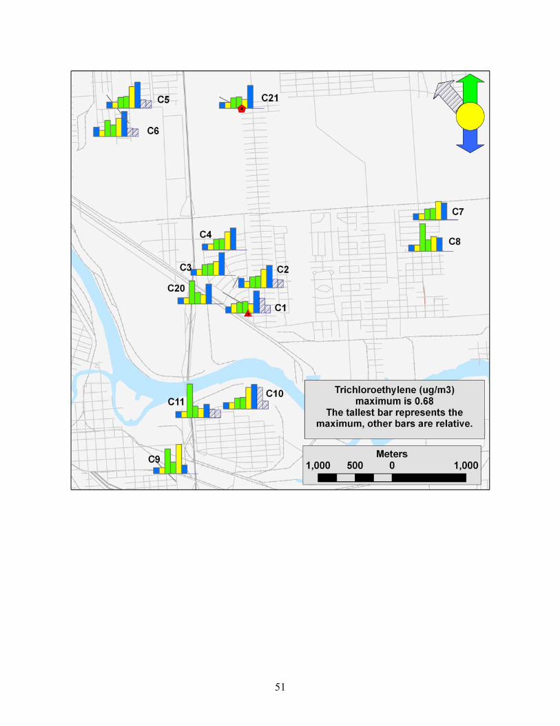
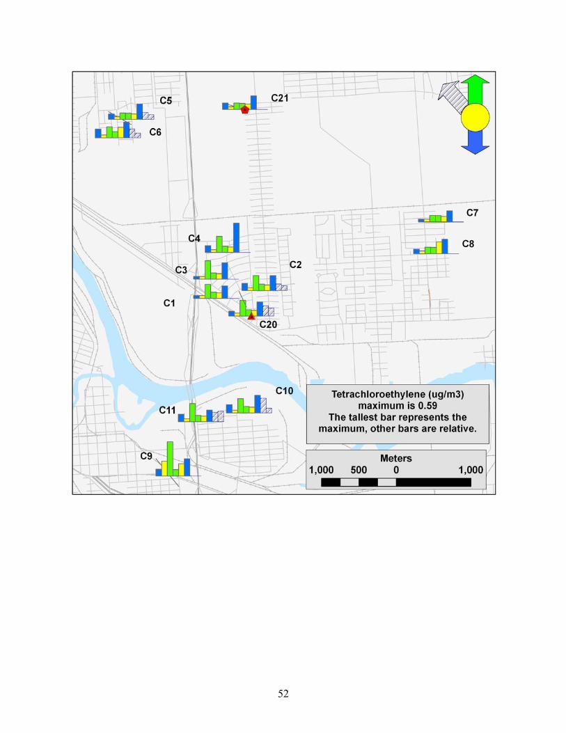
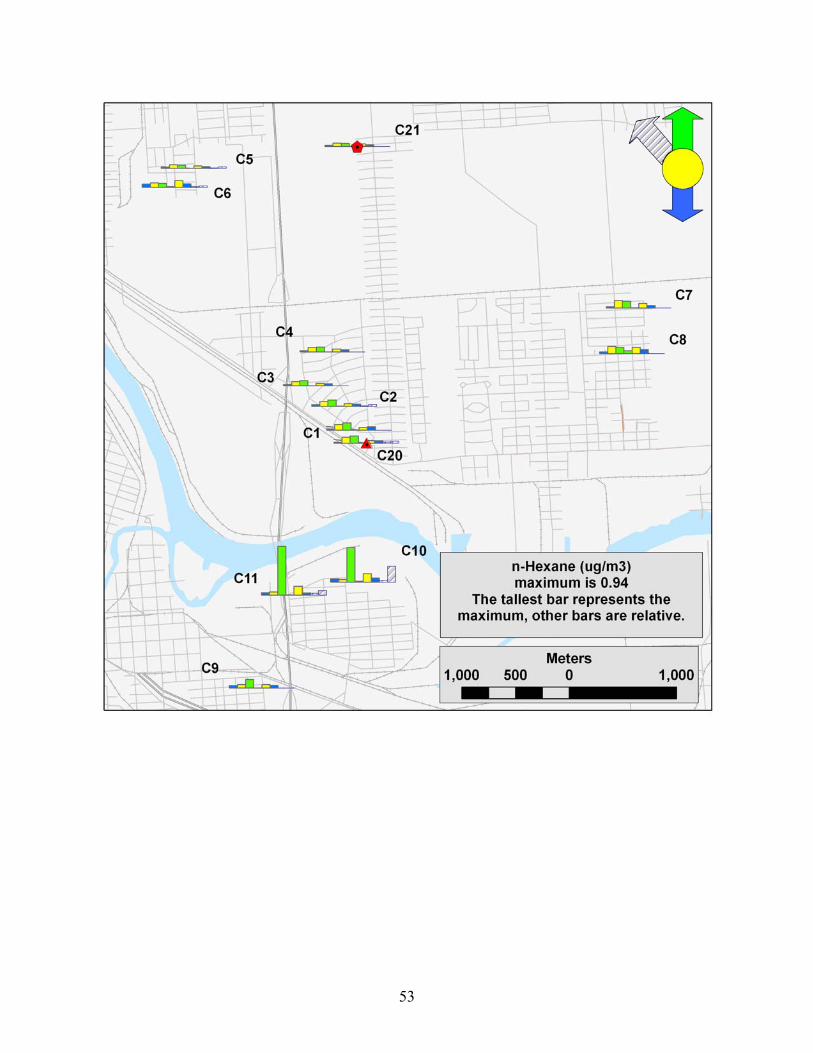
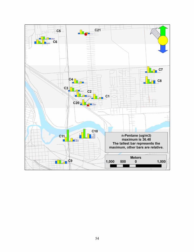
APPENDIX C – WARM AND COOL WEATHER CONCENTRATIONS FOR INDIVIDUAL CHEMICALS AT THE