Passive and active bodies in vortex-street wakes

J. Fluid Mech. (2010), vol. 642, pp. 95–125. c© Cambridge University Press 2009

doi:10.1017/S0022112009991741

95

Passive and active bodies in vortex-street wakes

SILAS ALBEN†School of Mathematics, Georgia Institute of Technology, Atlanta, GA 30332-0160, USA

(Received 6 February 2009; revised 14 August 2009; accepted 14 August 2009;

first published online 2 December 2009)

We model the swimming of a finite body in a vortex street using vortex sheetsdistributed along the body and in a wake emanating from its trailing edge. Wedetermine the magnitudes and distributions of vorticity and pressure loading on thebody as functions of the strengths and spacings of the vortices. We then consider themotion of a flexible body clamped at its leading edge in the vortex street as a modelfor a flag in a vortex street and find alternating bands of thrust and drag for varyingwavenumber. We consider a flexible body driven at its leading edge as a model fortail-fin swimming and determine optimal motions with respect to the phase betweenthe body’s trailing edge and the vortex street. For short bodies maximizing thrustor efficiency, we find maximum deflections shifted in phase by 90◦ from oncomingvortices. For long bodies, leading-edge driving should reach maximum amplitudewhen the vortices are phase-shifted from the trailing edge by 45◦ (to maximize thrust)and by 135◦ (to maximize efficiency). Optimal phases for intermediate lengths showsmooth transitions between these values. The optimal motion of a body driven alongits entire length is similar to that of the model tail fin driven only at its leadingedge, but with an additional outward curvature near the leading edge. The similaritybetween optimal motions forced at the leading edge and all along the body supportsthe high performance attributed to fin-based motions.

Key words: propulsion, swimming/flying, vortex streets

1. IntroductionClassical works on the mechanics of fish locomotion have studied how periodic

undulating motions along the fish body can generate propulsion in a quiescentinviscid fluid (Lighthill 1969; Wu 1971). In many real situations the flow is disturbedby upstream objects (including other swimming fish) before it encounters an individualswimming fish. Recently Liao et al. (2003) studied a trout swimming in the alternating(von Karman) street behind an upstream D-cylinder while maintaining its streamwisedistance from the D-cylinder. They observed that the trout slaloms around eachoncoming vortex in the street, using a body–tail-fin swimming motion. Earlier,Streitlien, Triantafyllou & Triantafyllou (1996) had studied a computational modelof a rigid aerofoil moving in an idealized von Karman street. The foil sheds vorticesin discrete clusters according to the Kutta condition of finite velocity at the trailingedge. They found that for certain parameters, the foil may gain larger thrust bymoving towards the oncoming vortices instead of slaloming around them. Otherexperiments (Abrahams & Colgan 1987; Weimerskirch et al. 2001) and theoreticalmodels (Lissaman & Shollenberger 1970; Weihs 1973; Wu & Chwang 1975) have

† Email address for correspondence: [email protected]

96 S. Alben

studied the locomotion of arrays of birds and fish and have examined the energysavings as a function of the spacings between individuals.

In Streitlien et al. (1996) and Liao et al. (2003), the swimming motion is frequency-locked to the vortex street. The motion can then be characterized by the spatial phasebetween the transverse displacement of the body (where it takes its maximum, orat a particular location such as the trailing edge) and the vortex street. In anotherwork Alben (2009), we have studied the swimming of a periodic body in a vortexstreet. Periodic boundary conditions simplify the equations considerably and allowfor exact solutions to certain optimal swimming problems and the determination ofthe scalings of physical quantities of interest (such as thrust force and efficiency) withrespect to parameters. Forces on the body arise from the no-penetration condition,which requires the normal motion of the fluid to match the normal motion of thebody. The consequent acceleration of fluid in the downstream direction provides athrust force on the body. This periodic model neglects the important phenomenon ofthe shedding of vorticity by the sharp trailing edge of a finite body. Such vorticityis an important contribution to the drag forces on a finite body (Saffman 1992). Forthe periodic model, we have found that thrust is maximum when the phase differencebetween the vortices and the body motion ranges from 0◦ to 90◦. It is 0◦ for a narrowvortex street and transitions smoothly to 90◦ when the vortex street is moderatelywide (compared to the streamwise spacing between adjacent vortices).

In the present work, we consider a finite body which sheds a trailing vortex wakein accordance with the Kutta condition (Batchelor 1967; Jones 2003). We find thatthe optimal phase of the body motion is determined in part by the position of thetrailing edge with respect to the vortices. For bodies which are short or long relativeto the vortex spacing, well-defined optimal phases arise. For bodies of intermediatelengths, the optimal phase smoothly interpolates these limiting phases.

The outline of the paper is as follows. In § 2 we present the model for a finitebody moving in the potential flow of the vortex street. We derive the distribution ofvorticity along the body and in the wake and the distribution of pressure forces alongthe body. In § 3 we consider how passive and active flexible bodies (clamped or drivenat the leading edge) move and obtain thrust under such pressure forcing. For smallbody displacements, the problem can be decomposed into three linear problems –a driven body in a uniform flow (considered previously in Alben 2008a), a passiveelastic body (akin to a passive flag) driven by the point vortices and a beam drivenat the leading edge superposed with the flow and pressure distribution of the vortexstreet. We determine the magnitudes of the main flow quantities; for the case ofshort-wavelength vortex streets, this requires re-centring the co-ordinate system at thebody’s trailing edge. In § 4 we consider the optimal swimming motion of a body withfully prescribed shape, in terms of the maximum thrust force and efficiency. Section 5discusses the results in the context of previous studies.

2. Flexible body and trailing wake in a vortex streetWe consider a flexible body of length 2L in a periodic von Karman vortex street.

The street consists of two alternating rows of vortices (see figure 1). The top row hasidentical point vortices, each with circulation Γ , at the points {ml + id/2, m ∈ �}.The bottom row has vortices with circulation −Γ located at the points {(m + 1/2)l −id/2, m ∈ �}. The spacing between neighbouring vortices in a row is then l, andthe width of the vortex street is d . For the von Karman street, Γ < 0, while forthe inverse von Karman street, Γ > 0 (positive Γ corresponds to counterclockwise

Passive and active bodies in vortex-street wakes 97

–31/2 –1/2 1/2 1–L L–1 0

0

d/2

–d/2–Γ

Γ

h(x, t)

Figure 1. The parameters for a body of length 2L (solid line) swimming with amplitudeh(x, t) in a vortex street (bold stars) with width d and horizontal spacing between vortices l.The horizontal position of the body is assumed to be fixed (similar to that in Barrett et al.1999), but the vertical deflection varies in time either passively (due to fluid forces) or actively(a prescribed vertical motion at the leading edge or all along the body, which yields a force onthe body in the −ex-direction). At subsequent times the vortex street moves rightward (lightstars) due to the superposition of the velocity induced by the street on itself together with abackground flow velocity U ex .

rotation). We assume that the point vortices are superposed on a background flowwith uniform speed U . Such is the case when vortices are shed from a stationaryobstacle in a uniform stream or from an upstream body swimming at constant speedthrough quiescent fluid. In the latter case the background flow velocity is the negativeof the upstream body velocity, when we view the vortex street in a reference frametranslating with the upstream swimming body. In the unbounded plane, the vortexstreet translates with uniform velocity Ucex (Saffman 1992):

Uc = U + (Γ/2l) tanh(πd/l). (2.1)

We now introduce a body in the form of a flexible sheet along the midline betweenthe two alternating rows of vortices. The sheet executes small-amplitude displacementsh(x, t) transverse to the midline and thus has complex position x+ih(x, t). We assume|h| � d, l, L for the sake of analytical tractability, as explained below. We considerfirst the undeflected base state in which the solid sheet lies exactly along the x-axis.The condition that fluid does not penetrate the body can be satisfied by posing avortex sheet, or equivalently a jump in tangential velocity, across the body. We alsointroduce a vortex-sheet wake emanating from the trailing edge of the body. Thestrength of the vortex-sheet wake at the trailing edge is chosen at each instant tosatisfy the condition of finite flow velocity at the trailing edge – the ‘Kutta’ condition(Thwaites 1987; Bisplinghoff & Ashley 2002; Jones 2003). As a consequence, thevortex-sheet strength is continuous where the vortex wake meets the body at itstrailing edge.

We now determine the unsteady strength distribution of the vortex sheet on the bodyand in the wake. We may use the results to compute the pressure forces on the bodyfrom the Euler equations and the deflection of a passive flexible body using theEuler–Bernoulli equation of beam bending.

98 S. Alben

When one vortex in the translating upper row of vortices crosses the y-axis (shownby the bold stars in figure 1), the flow has the following complex velocity potential(Saffman 1992):

w = Uz − iΓ

2πlog

(sin

(π

l

(z − id

2

)))+

iΓ

2πlog

(sin

(π

l

(z +

l

2+

id

2

))). (2.2)

The complex-conjugate velocity is

u − iv =dw

dz= U − iΓ

2lcot

(π

l

(z − id

2

))+

iΓ

2lcot

(π

l

(z +

l

2+

id

2

)). (2.3)

Evaluating (2.3) at z = x and simplifying, we find that the point vortices induce thefollowing velocity on the x-axis:

u − iv∣∣∣y=0

= U − iΓ

l

cosh(πd/l)

sin(2πx/l) − i sinh(πd/l). (2.4)

So far we have assumed the particular instant in time at which one of the upperrow of vortices crosses the y-axis. If we assume this occurs at time t = 0, then atsubsequent times the complex velocity is given by (2.4) but with x changed to x −Uct .This distribution of velocity is then a travelling wave moving with speed Uc. Separatedinto real and imaginary parts, the time-dependent form of (2.4) is

u

∣∣∣y=0

= U +Γ

l

sinh(πd/l) cosh(πd/l)

sin2(2π(x − Uct)/l) + sinh2(πd/l), (2.5)

v

∣∣∣y=0

=Γ

l

sin(2π(x − Uct)/l) cosh(πd/l)

sin2(2π(x − Uct)/l) + sinh2(πd/l). (2.6)

We now consider the case in which d/l � 1/π, which includes physically reasonablevortex streets of moderate-to-large aspect ratio. Then (2.5) and (2.6) simplify to

u

∣∣∣y=0

= um(1 + O(e−2πd/l)), um = U +Γ

l; (2.7)

v

∣∣∣y=0

= vm(1 + O(e−2πd/l)), vm(x, t) =2Γ

le−πd/l sin(2π(x − Uct)/l). (2.8)

We express vm as the real part of a complex exponential:

vm(x, t) = Re(Vm(x)eiωt ); Vm(x) =2iΓ

le−πd/le−2πix/l; ω = 2πUc/l. (2.9)

The no-penetration condition on the body takes the form

vm(x, t) +1

2π

∫ L

−L

γ (x ′, t)dx ′

x − x ′ +1

2π

∫ ∞

L

γ (x ′, t)dx ′

x − ζ (x ′, t)= 0, −L < x < L. (2.10)

Here ζ (x ′, t) is the complex position of the free vortex sheet, and we have neglectedterms which are O(h, ∂xh). This equation states that on the body, the vertical flowvelocity due to the point-vortex street and the body and wake vortex sheets equalsthe vertical velocity of the body, which is zero in the base state where the body is aflat plate.

The vortex-sheet wake ζ (x, t) is a contour in the complex plane which emanatescontinually from the trailing edge and is advected passively by the local fluid flow atζ . We define the circulation in the vortex-sheet wake as an integral of the vortex-sheet


strength:

Γ (x, t) =

∫ x

∞γ (x ′, t)dx ′, L < x < ∞. (2.11)

At each material point of the vortex-sheet wake, the circulation Γ is conserved intime (Saffman 1992) and is equal to the value of circulation it had at the initiation ofthe material point at the trailing edge of the body at a time t∗ (Krasny 1991; Jones2003). Thus

Γ (x, t) = Γ (L, t∗(x)), L < x < ∞. (2.12)

The initiation time t∗ has a unique value for each position x on the vortex-sheet wake.We now argue that the assumption d/l � 1/π also simplifies the vortex wake

dynamics and thus simplifies the last integral in (2.10). First, we note that vm isO(e−πd/l). By its continuity at the trailing edge, γ is of the same order in d/l onthe body and in the vortex-sheet wake. By (2.10), on both contours γ is of thesame order as vm, O(e−πd/l). The local fluid flow at points on the vortex-sheet wakeis a superposition of four flows: the horizontal background flow U and the flowsinduced by the vortex sheet along the body, the vortex sheet along the wake andthe point-vortex street. We assume that body is inserted into the vortex street at aninitial time (t0, say), and then the vortex-sheet wake emanates steadily under the flowat the trailing edge. The horizontal flow is um, and the vertical velocity there fromthe vortex street (vm) and from the body’s vortex sheet is O(e−πd/l). Thus to leadingorder the vortex sheet emanates horizontally from the body. At all subsequent timesthe horizontal velocity on the sheet is um +O(e−πd/l), and the vertical velocity remainsO(e−πd/l). Thus for long times, at leading order in powers of e−πd/l with πd/l � 1, wemay approximate the vortex-sheet wake as a semi-infinite horizontal line extendingfrom x = L to x = ∞. It may be shown that the velocity induced at the point vorticesin the vortex street is also O(e−πd/l); so we may reasonably assume (as observed inthe experiment of Liao et al. 2003) that insertion of the body into the vortex streetdoes not modify it at leading order.

The distribution of vorticity γ in the vortex-sheet wake is also simplified becausethe problem is time-periodic at leading order. The velocity of the point-vortex streetequals Uc + O(e−πd/l) and is thus steady and horizontal at leading order. By (2.9)and (2.10) (with ζ (x ′, t) = x ′ now), the problem is periodic with a single frequencyω = 2πUc/l. Thus the total circulation in the wake is a periodic function:

Γ (L, t) = Γ0eiωt . (2.13)

Because the wake moves horizontally at constant speed, the distribution of circulation(and vorticity) in the vortex-sheet wake is spatially periodic:

Γ (x, t) = Γ (L, t∗(x)) = Γ

(L, t − x − L

um

)= Γ0e

iωte−iω(x−L)/um, L < x < ∞. (2.14)

It is most convenient mathematically to non-dimensionalize all lengths by L (thebody half-width) and time by l/Uc (the temporal period of the vortex-street motion).

100 S. Alben

Then (2.14) yields

Γ (x, t) = Γ0ei2πte−iΩ(x−1), 1 < x < ∞, (2.15)

γ (x, t) = ∂xΓ (x, t) = G(x)ei2πt , 1 < x < ∞, (2.16)

G(x) = −iΩΓ0e−iΩ(x−1), 1 < x < ∞, (2.17)

Ω =ωL

um

=2πUc

um

L

l=

2πL

l

1 +1

2(Γ/lU )

1 + (Γ/lU ), (2.18)

where the dependent and independent variables (including Γ0) in (2.15)–(2.17) arenow dimensionless. Equation (2.10) then becomes

1

2π

∫ 1

−1

G(x ′)dx ′

x − x ′ = F (x), −1 < x < 1, (2.19)

F (x) = −Vm(x) − Γ0E(x), (2.20)

E(x) = − iΩ

2π

∫ ∞

1

e−iΩ(x′−1)dx ′

x − x ′ , (2.21)

Vm(x) = 2iΓ/lU

1 + 12Γ/lU

l

Le−2πixL/le−πd/l (2.22)

where all variables are again dimensionless. There are two unknowns to be found: Γ0

and G(x). Similar to Jones (2003), we explicitly remove the logarithmic singularity inF (x) at x = 1:

F (x) = f (x) +iΩΓ0

2πlog(1 − x), (2.23)

where f is a bounded continuous function. We can solve (2.19) for G in terms of aChebyshev expansion of f :

f (x) =

∞∑k=0

fk cos kθ ; θ = arccos x. (2.24)

The solution to (2.19) is then

V (θ) =2

∞∑k=1

fk sin kθ sin θ − f1 − 2f0 cos θ (2.25)

+iΩΓ0

π(1 − (π − θ) sin θ + log(2) cos θ) + C; G(θ) = V (θ)/ sin θ. (2.26)

Here we have evaluated the Hilbert transform of log(1 − x) in closed form usingMathematica 6. The constant C is set by the conservation of circulation (Kelvin’sTheorem), ∫ 1

−1

γ (x, t)dx − Γ (1, t) = 0, (2.27)

which implies that C = Γ0/π, using (2.26). Solution (2.26) for the bound vorticity G

is continuous with the vorticity in the vortex-sheet wake at x = 1; both equal the realpart of −iΩΓ0e

i2πt . We can solve for the total circulation in the wake Γ0 explicitlyusing the Kutta condition that velocity (and therefore γ and G) are finite at thebody’s trailing edge. By (2.26) for G, V must be zero at θ = 0. Then by (2.25) for V ,

Γ0

π(1 + iΩ(1 + log(2))) = f1 + 2f0. (2.28)


00

0

0

1

–1

–1

–1

–2

–2

–2–3

–3

–3

–4

4

–5

–5

–6

1

1

2

2

23

3

4

log10 l/L

log

10Γ

/lU

0 1 2 3

0

1

–1

–2

–3

–4–2 –1

2

3

Figure 2. Contours of constant log10 |Γ0|eπd/l in the space of the point vortices’ strength|Γ |/lU and their horizontal spacing l/L. The normalizing factor eπd/l is included to removedependence on d/l.

Using (2.23) and (2.20),

Γ0 =−2

∫ 1

−1Vm(x)

√1 + x

1 − xdx

1 + iΩ(1 + log(2)) + 2∫ 1

−1

[E(x) + iΩ

2πlog(1 − x)

] √1 + x

1 − xdx

. (2.29)

The integrands in (2.29) are bounded when the variable of integration is changedfrom x to θ . In figure 2 we plot contours of the strength of the shed sheet, |Γ0|, withrespect to the strength of the vortices, |Γ |/lU , and their horizontal spacing relativeto the plate length l/L. There are four asymptotic regimes which can be deducedfrom (2.29). The integrals in the numerator and denominator both involve weightedintegrals of e−2πiLx/l . When l/L � 1, both integrals are O(1) in l/L. Then |Γ0| ∼l/L, from the l/L prefactor in Vm. When l/L � 1, both integrals are O((l/L)−1/2)(shown in § 3.4, (3.35)). Then |Γ0| ∼ (l/L)2, from the l/L prefactor in Vm and theterms proportional to Ω ∼ L/l in the denominator. Then |Γ0| has the followingscalings:

|Γ0| ∼ e−πd/l |Γ |/lU

1 + 12Γ/lU

(l

L

)2

,l

L� 1; |Γ0| ∼ e−πd/l |Γ |/lU

1 +1

2Γ/lU

l

L,

l

L� 1. (2.30)

These asymptotic scalings are verified in figure 2, a contour plot of |Γ0| computednumerically. We have assumed that Γ/lU , if negative, is less than 2, so that advectionof the vortex street is not dominated by the self-induction of the vortices relative tothe background flow – which is physically reasonable for most wake flows (Batchelor1967).

Physically, |Γ0| grows with |Γ |/lU because the strength of vorticity on the bodyand in the wake must be strong enough to offset the flow due to the point vortices,from the no-penetration condition. When |Γ |/lU is large, |Γ0| saturates because it isnon-dimensionalized using the speed Uc of the point vortex street, which grows with

102 S. Alben

|Γ |/lU when |Γ |/lU is large; |Γ0| has the same linear dependence on l/L as does thenormal flow Vm when l/L is large. When l/L is small, rapid oscillations in the normalflow cancel to some extent in the vorticity induced by the normal flow, and thus |Γ0|tends to zero as (l/L)2, more rapidly than Vm.

Having solved for Γ0 (2.29), we now have the vortex-sheet strength in the wake.Using (2.26) we also have the solution for G(x), the vortex-sheet strength on the body.From (2.26), the magnitude of G is the sum of the terms with the same magnitude asVm and the terms proportional to Γ0. Thus the magnitude of G is the same as Vm forl/L large and small (in which case the Γ0 terms become subdominant):

|G| ∼ e−πd/l |Γ |/lU

1 +1

2Γ/lU

l

L. (2.31)

We may derive the difference in pressure across the body in terms of γ , which isthe same as the difference in fluid pressure across a generic vortex sheet, derived bySaffman (1992) using the Euler equations expressed on either side of the body. Theresult is

1

ρf

∂s[p] = ∂tγ + ∂s((μ − τ )γ ), (2.32)

where ρf is the fluid density per unit area; s is arclength along the body; μ is thetangential component of the average of the fluid velocities on either side of the body;and τ is the component of the body velocity along its tangent. For a static, horizontalbody lying in −1 < x < 1,

1

ρf

∂x[p] = ∂tγ +

(U +

Γ

l

)∂xγ, (2.33)

where we have set μ equal to the constant um in (2.7). We non-dimensionalize [p] byρf U 2

c (L/l)2, and then in dimensionless form (2.33) is

∂x[p] = ∂tγ +1 + Γ/lU

1 +1

2Γ/lU

l

L∂xγ. (2.34)

Separating out the harmonic time dependence of [p],

[p](x, t) = P (x)ei2πt , (2.35)

(2.33) becomes

∂xP = i2πG +1 + Γ/lU

1 +1

2Γ/lU

l

L∂xG. (2.36)

We integrate (2.36) with the boundary condition that the pressure jump vanishes atthe trailing edge,

P

∣∣∣x=1

= 0, (2.37)

to obtain

P (x) = i2π

∫ x

1

G(x ′) dx ′ +1 + Γ/lU

1 + 12Γ/lU

l

L(G(x) + iΩΓ0), (2.38)

where we have used G(1) = −iΩΓ0. For l/L � 1, both terms on the right-hand sideof (2.38) are O((l/L)2). For l/L � 1, the second term dominates the first by O((l/L)2)


0

0

0.5

–0.5

–0.2

–0.4

–1.0 –0.5 0 0.5 1.0

G/(

le–π d

/l/L

)P

/(l2

e–π d

/l/L

2)

(a)

(b)

x

Figure 3. (a) The bound vorticity G and (b) the pressure P for two different values of l/L:0.1 and 1. The wavelength of the shapes is proportional to l/L. The solid lines give thecos(2πt + φT E) component, and the dashed lines give the − sin(2πt + φT E) component, wherethe phase shift φT E (3.33) is applied to give convergence at both small and large l/L; P ismultiplied by eπd/l/(l/L)2 and G is multiplied by eπd/l/(l/L), so the amplitudes do not changeas d/l and l/L are varied. The value of Γ/lU is 0.1. Different values of Γ/lU mainly modifythe amplitudes but not the shapes of G and P .

versus O((l/L)). Thus for l/L small and large,

|P | ∼ e−πd/l |Γ |/lU

1 + 12Γ/lU

(l

L

)2

. (2.39)

Having determined the magnitudes of Γ0, G and P with respect to the dimensionlessparameters, we now discuss the functional forms of G and P .

In figure 3 we plot G and P for small-to-moderate values of l/L. As statedpreviously, we are considering the regime in which πd/l is greater than one. Herewe set Γ/lU = 0.1, corresponding to a somewhat weak reverse von Karman vortexstreet, and address changes due to varying Γ/lU subsequently. Furthermore, we adda phase shift φT E to the functions so that the solid line in figure 3 corresponds toalignment of a vortex from the upper street with the trailing edge of the body (insteadof its midpoint as for the bold stars in figure 1), and the dashed line is shifted by 90◦

from that phase. We have thus plotted the real and imaginary parts of P eiφT E

, whichconverges in the limits of small l/L and large l/L, as explained further in § 3.4, (3.33)and (3.37).

For small l/L (figure 3a), G is essentially sinusoidal, apart from regions nearthe end points which shrink as l/L decreases. The reason that G is sinusoidal forsmall l/L may be seen in (2.19) and (2.20) with Vm given in (2.22). We have alreadynoted in (2.30) that Γ0 tends to zero like (l/L)2 when l/L is small. Thus it becomessubdominant to Vm on the right-hand side of (2.19); so the flow induced by thevortex-sheet wake is subdominant to the flow induced by the point vortices, awayfrom the ends by more than O(l/L). We now recall that Vm is proportional to e−2πiLx/l .

104 S. Alben

Using the definition of the exponential integral with an imaginary argument Ei(ix)and its asymptotic behaviour for large x,

∫ 1

−1

eikx′dx ′

x − x ′ = eikx [iπ sign(k) + Ei(−ik(1 + x)) − Ei(ik(1 − x))] , −1 < x < 1, (2.40)

∫ 1

−1

eikx′dx ′

x − x ′ ∼ eikx [−iπ sign(k)] + O

(1

k

), k � 1, 1 ± x � 1

k. (2.41)

Equation (2.41) shows that the integral on [−1, 1] behaves the same way as does theHilbert transform on [−∞, ∞] for large k, away from small end regions. Since Vm isa complex exponential with k = −2πL/l, (2.41) shows that G has the same form forlarge k (small l/L):

G = 4Γ/lU

1 +1

2Γ/lU

l

Le−2πiLx/le−πd/l + O

(l

L

)2

, 1 ± x � L

l. (2.42)

This form agrees well with figure 3(a). The asymptotic relation (2.41) may also beused to explain the good agreement between the stability diagram of a finite and aninfinite flapping flag for small bending rigidity, when large-wavenumber shapes occur(Shelley, Vandenberghe & Zhang 2005; Alben 2008b). Furthermore, (2.41) may beused to relate vortex-sheet problems with a finite boundary to those with periodic orinfinite boundary conditions (Hou, Lowengrub & Shelley 2001; Ambrose & Wilkening2008; Alben 2009), where the Hilbert transform is simpler in Fourier space. Physically,when the wavelength of the flow on the body is much shorter than the body length,the end conditions (finite or infinite) become less important. A similar asymptoticbehaviour was found in studies of a flexible body driven periodically in a fluid stream(Alben 2008a) and the second-order bending of a flexible fibre in a steady flow(Alben, Shelley & Zhang 2004).

We now consider the pressure at small l/L (figure 3b). The pressure is a linearcombination of G and an integral of G (2.38). It is a sinusoidal shape superposedon a longer-wavelength background shape which diverges at the leading edge. Thebackground shape tends to zero as l/L tends to zero, leaving a sinusoidal pressureover the whole body, except in small regions near the leading and trailing edges.

In figure 4 we show G and P at large l/L. They converge to shapes which dependon the function E(x) in equation (2.21), and which are independent of l/L in thislimit. The solid line in figure 4(a) is nearly zero away from the leading edge. Thisis the bound vorticity induced when the body trailing edge is aligned with a pointvortex from the upper street. The near symmetry of the vortex configuration in thissituation means that the normal flow is very small on the body. At the leading edgeG diverges like an inverse square root, though with a small prefactor at this phase.The dashed line is nearly linear over the middle region of the body. This is thebound vorticity induced when the body trailing edge lies midway between the nearestvortices from the upper and the lower street. Then the contribution to the normalflow from the nearest vortices in each street adds constructively, yielding a maximumof bound vorticity. Because l/L is large, the normal flow is nearly uniform over the(small) body and is cancelled by a linear distribution of bound vorticity. Hence thedashed line in figure 4(a) is approximately linear on the central portion of the body.There is a deviation to a square-root behaviour at the trailing edge and an inversesquare-root divergence at the leading edge. Because the flow from the point vortices


0

–1

–2

1

0

–1

–2–1.0 –0.5

1

0 0.5 1.0x

(b)

(a)G

/(le

–π d

/l/L

)P

/(l2

e–π d

/l/L

2)

Figure 4. (a) The bound vorticity G and (b) the pressure P for five different values of l/L:10 to 105 in integral powers of 10. Lines for the three largest values of l/L = 103, 104, and 105

show convergence to a single line which is slightly thicker than the others. The other plottingdetails are the same as for figure 3.

is larger in the imaginary phase than in the real phase, the prefactor of the divergenceis also much larger in this case.

In figure 4(b), the pressure is nearly identical to the bound vorticity (figure 4a)times a factor of l/L. This is because the second term in (2.38) dominates the first(the integral term) for large l/L.

3. Body driven (or clamped) at the leading edgeWe now consider an elastic body placed in the flow. The body is assumed to be

clamped (held with zero vertical displacement and tangent angle) or driven at theleading edge and free at the trailing edge. Such a body yields a model for the tailfin of a fish swimming in a vortex street, which occurs when the fin lies in the wakeof an obstacle (Liao et al. 2003), of another fin on the same fish (i.e. the dorsal fin;Drucker & Lauder 2001, 2005) or of another fish while swimming in a school (Weihs1973). Because the flow induced by the vortex street is sinusoidal for wide vortexstreets, this model may also be used to study the effect of generic fluid disturbanceson the fin through Fourier decomposition.

The fin shape is ζ (x, t) = x + ih(x, t). We assume small deflections, so |h|, |∂xh| � 1.We also assume spatially uniform rigidity, for simplicity (but see Alben, Madden &Lauder 2007). The fin moves according to the linear beam equation and is forced bythe pressure of the undisturbed vortex street:

R1∂tth(x, t) = −R2∂xxxxh(x, t) − [p]. (3.1)

Here R1 and R2 are the dimensionless mass per unit length and bending rigidity ofthe fin:

R1 =ρs

ρf L; R2 =

B

ρf U 2c L3

l2

L2. (3.2)

106 S. Alben

Assuming a solution with the same temporal period as the vortex street,

h(x, t) = H (x)ei2πt , (3.3)

and (3.1) becomes a linear inhomogeneous ordinary differential equation (ODE):

−(2π)2R1H + R2∂xxxxH = −P. (3.4)

We now assume the fin is driven at its leading edge with a combination of heavingand pitching (Lighthill 1969):

H (−1) = H0eiφH ; H ′(−1) = Θ0e

iφθ H ′′(1) = H ′′′(1) = 0. (3.5)

The heave and pitch amplitudes H0 and Θ0 are non-negative numbers. The heave andpitch phases φH and φθ give the time, in units of 2π times the period, by which theheaving or pitching maximum precedes the passage of a point vortex from the upperstreet over the midpoint of the body.

3.1. Feedback from body motion on to pressure

In § 2 we derived the pressure jump P on a body which undergoes zero deflection.Now we consider how the solution to the flow–body problem, including P in (3.4),changes when the body is in motion. We assume the body deflection is no longerzero but is small (|H |, |∂xH | � 1). Feedback from the body motion to the flow isobtained by allowing the body motion to alter the vorticity induced on the body andin the wake and therefore also the pressure on the body. In this case, still linearizedfor small amplitudes, (2.10) and (2.19) are modified to read

(∂t + U∂x)h(x, t) = vm(x, t) +1

2π

∫ L

−L

γ (x ′, t)dx ′

x − x ′

+1

2π

∫ ∞

L

γ (x ′, t)dx ′

x − ζ (x ′, t), −L < x < L, (3.6)

1

2π

∫ 1

−1

G(x ′)dx ′

x − x ′ = 2πiH (x) +U

Uc

l

LH ′(x) − Vm(x) − Γ0E(x), −1 < x < 1. (3.7)

The terms in (3.6) and (3.7) involving h and H are new, but we have neglectedterms which are O(γ h, γ ∂xh). We may decompose solutions (Gm, Γ0m, Pm, Hm) to themodified kinematic equation (3.7) plus the beam equation (3.4) and pressure equation(2.36) into a sum of two solutions:

(Gm, Γ0m, Pm, Hm) = (G, Γ0, P , H ) + (Gh, Γ0h, Ph, Hh). (3.8)

The terms (G, Γ0, P , H ) are the solutions to (2.19) (unmodified by body motion) plus(3.4) and (2.38); (Gh, Γ0h, Ph, Hh) solve the part of (3.7) with body coupling to theflow (the H terms) but without the vortex street (Vm),

1

2π

∫ 1

−1

Gh(x′)dx ′

x − x ′ = 2πiHh(x) +U

Uc

l

LH ′

h(x) − Γ0hE(x), −1 < x < 1. (3.9)

The terms (Gh, Γ0h, Ph, Hh) are then the solution for a body driven or clamped atthe leading edge in a fluid stream. This problem was addressed in a previous work(Alben 2008a). The solutions were found to be akin to those of a damped drivenoscillator, where the fluid is a source of both damping and excitation, leading todamped resonances at certain values of R2. The only difference in Hh here is thatthe constant advection speed in (2.33) is now U + Γ/l instead of U in the previouswork. The structure of the solutions is essentially the same and becomes exactly the


same for weak vortex streets, Γ/lU � 1. Thus for small deflections, the solution isa superposition of the damped-driven beam of Alben (2008a) with the ‘decoupled’solution (G, Γ0, P , H ) in which the body is moved by the flow of a vortex street overa flat plate, but the flow is unmodified by body motion. Only the decoupled solutiondepends on the vortex street, and is not yet known, so we focus on it in this work.The problem of maximizing thrust or efficiency then becomes the problem of thesetting the body shape to optimally ‘catch the breeze’ from the passing vortex street.More precisely, this means setting the body slope relative to the pressure induced bythe vortex street to yield a force in the upstream direction.

The decoupled solution is also the leading-order solution in a particular asymptoticlimit. In the limit that R1 and R2 are large relative to the magnitude of P , the bodyis too stiff or heavy to deflect much under the vortex pressure loading. The bodyshape may then be expanded as a formal asymptotic series in inverse powers of R1

and R2 times a function of the flow parameters d/l, l/L and Γ/lU . Although we donot pursue it further in this work, the form of this expansion can be found from thesolution to the decoupled problem, which we give next.

3.2. Body driven at the leading edge

The solution to (3.4) with boundary conditions (3.5) is the classical variation-of-parameters solution for a linear ODE:

H (x) = C1e−kx + C2e

kx + C3 sin(kx) + C4 cos(kx)

+k−3

2R2

[e−kx

2

∫ x

−1

ekx′P (x ′)dx ′ − ekx

2

∫ x

−1

e−kx′P (x ′)dx ′

− cos(kx)

∫ x

−1

sin(kx ′)P (x ′)dx ′ + sin(kx)

∫ x

−1

cos(kx ′)P (x ′)dx ′]

, (3.10)

k = (2π)1/2(R1/R2)1/4. (3.11)

Here k is the characteristic wavenumber for the neutral oscillations of an elasticrod with mass in a vacuum. The constants C1, C2, C3, C4 are chosen to satisfy theboundary conditions in (3.5) and are given in the Appendix . The solution is

H (x) = H1(x) + H2(x), (3.12)

a superposition of two solutions. The function H1(x) is the solution to the equationwith homogeneous boundary conditions. This is the part of solution (3.10) involvingP , with all the terms proportional to H0 and Θ0 set to zero, and is the motion ofa passive body clamped at the leading edge and driven by the vortex street. Thefunction H2(x) is the solution to the homogeneous equation

−(2π)2R1H2 + R2∂xxxxH2 = 0, (3.13)

with the driving boundary conditions (3.5); H2 is the part of (3.10) involving H0 andΘ0, with the terms involving P set to zero.

We can quantify when the criteria (|H | � 1, |∂xH | � 1) are met in terms of solution(3.10). For the part of the solution which depends on H0 and Θ0, we require that

H0,Θ0

k� 1 (3.14)

for small deflections and

kH0, Θ0 � 1 (3.15)

108 S. Alben

for small slopes. For the part of the solution which depends on P , solution (3.10)shows that body deflection magnitudes are proportional to R−1

1 times an integral ofthe pressure (with magnitude given in (2.39)). Hence the magnitude of H is

|H | ∼ 1

R1

e−πd/l |Γ |/lU

1 + 12Γ/lU

(l

L

)2

. (3.16)

Differentiating solution (3.10) introduces a factor of k; so body slope magnitudes aregiven by the right-hand side of (3.16) but with R−1

1 changed to R−3/41 R

−1/42 . Thus for

the linear theory we require

R1, R3/41 R

1/42 � e−πd/l |Γ |/lU

1 + 12Γ/lU

(l

L

)2

. (3.17)

Criteria (3.17) require the flow induced by the vortex street to be sufficiently weakrelative to the body mass and rigidity. The second term on the left side of (3.17) isproportional to R1/k. Thus, shapes of large wavenumbers are permitted provided R1

is sufficiently large.There is another criterion, in addition to (3.14), (3.15) and (3.17), which is necessary

for the body to undergo small deflections. The resonant frequency of the body mustnot coincide with the frequency of the vortex street. This occurs when

k = 0.9376, 2.3470, 3.9273, 5.4978, . . . , (3.18)

where subsequent terms in the k sequence are very nearly π/2 apart (see Alben 2008b).These are a sequence of lines with slope 1 in the R1–R2 plane.

We shall now consider the motion of the clamped body as a model for a flappingflag in a vortex street. When a flag becomes unstable to flapping, small-amplitudemotions grow until saturation, when nonlinear effects become important. Evenfor large-amplitude flapping, the small-amplitude, small-slope equations can be areasonable approximation to the large-amplitude flag dynamics, particularly for thelow-wavenumber flapping modes (Alben 2008b; Eloy et al. 2008). The model mayalso be applied to vortex-driven motions of stable passive bodies. The flapping-flaginstability does not occur in a large region of the R1–R2 space, which is givenapproximately by the criteria that R2 must be larger than 1 when R1 is larger than10 and R2 must be larger than 0.1R1 when R1 is less than 10 (Alben 2008b). Here R1

is the same as in (3.2), and R2 is the expression in (3.2) but with Uc changed to U

and the factor l2/L2 removed.Having described when we may expect the small-deflection theory to be valid, we

now consider the motion and forces experienced by a body clamped or driven at theleading edge. In § 3.3 we consider the clamped body, given by H1 in (3.12). Such abody yields a model for a flapping flag placed in a vortex street, which occurs whenthe flag lies in the wake of another object – such as a rigid obstacle (i.e. the flag pole),or another flapping flag (Ristroph & Zhang 2008), in which case Γ < 0, or a bodyswimming upstream, in which case Γ > 0. In § 3.4 we consider the body driven at theleading edge as a model for a flexible tail fin in a vortex street. The fin is modelled byH , a sum of H1 and H2 in (3.12). We shall show that the problem of optimal drivingat the leading edge is one of matching the driving phases to the phases of weightedintegrals of the pressure jump P .

3.3. Small perturbations of a passive body clamped at the leading edge

We now consider a passive elastic body, clamped at the leading edge and placed in avortex street, given by H1 in (3.12); H1 may be used alone or together with Hh (in (3.8),


0

0.2

–0.2

–0.4

0.4(a)

(b)

0 0.5 1.0

0

1

–1

2

–2–1.0 –0.5

x

H/(

l2e–

π d

/l/(

4π

2 R

1 L

2))

H/(

l2e–

π d

/l/(

4π

2 R

1 L

2))

Figure 5. The shape of a passive flexible body for (a) l/L = 1 and (b) l/L = 100 andfor k4/(2π)2 = R1/R2 = 10−2, 100, 102. Larger values correspond to higher-wavenumberdeformations. The solid lines give the cos 2πt component, and the dashed lines give the− sin 2πt component. Here Γ/lU is 0.1; for negative values small in magnitude, the shapes areessentially reversed in sign.

with clamped-free boundary conditions) to model a flapping flag in a vortex street.The superposition Hh + H1 gives the fully coupled flapping-flag dynamics (linearizedfor small deflections).

Equation (3.4) is solved by H1 solves with boundary conditions:

H1(−1) = H ′1(−1) = 0 ; H ′′

1 (1) = H ′′′1 (1) = 0. (3.19)

In figure 5, body shapes are plotted for different values of R1/R2 and l/L. Whilethe body amplitudes are proportional to 1/R1 (3.16), the body shapes depend onlyon the ratio R1/R2 or k, as can be seen in (3.10). The number of wavelengths onthe body increases by one half as k increases through each of the intervals betweenresonant values (3.18); the body shape reflects across the x-axis as k moves througha resonance. Solution (3.10) shows that for both large and small l/L, the bodyshapes are essentially a superposition of sinusoidal waves with wavenumber k withthe pressure jump. For small l/L, the sine and cosine components of the motion arenearly equal. As l/L becomes large, the sinusoidal component dominates due to thelarger pressure forcing at this phase (figure 4b).

The instantaneous horizontal force on the body due to the flow is given by

Fx = −π

8v(−1, t)2 +

∫ 1

−1

[p](x, t)∂xh(x, t)dx. (3.20)

The first term on the right of (3.20) represents the suction force on the leading edge ofthe body (Saffman 1992) and is the limit of the pressure force on a rounded edge as theedge becomes sharp (i.e. the curvature of the edge becomes infinite). The second termon the right side of (3.20) is the horizontal component of the pressure force on the

110 S. Alben

body. The period-averaged horizontal force is

〈Fx〉 = − π

16|V (−1)|2 +

1

2

∫ 1

−1

Re(P (x)∂xH (x))dx, (3.21)

〈Fx〉 = − π

16|V (−1)|2 +

1

2

∫ 1

−1

Re(((2π)2R1H − R2∂4xH )∂xH )dx, (3.22)

〈Fx〉 = − π

16|V (−1)|2 +

1

4(2π)2R1|H |2

∣∣∣1

− 1

4R2|H ′′|2

∣∣∣−1

(3.23)

where the bar in (3.21) denotes the complex conjugate. We have used integration byparts and the clamp boundary conditions (3.19) to simplify the equations, so onlyquantities at the boundaries are needed. The terms involving leading-edge suction andleading-edge curvature are negative and therefore provide thrust on the body, whilethe second term, involving trailing-edge deflection, is positive and thus contributes adrag force.

For a model of the flapping flag, the term H in (3.23) is a superposition of Hh andH1. For the more quantitative discussion of forces in the remainder of this section,we now neglect the term Hh and focus instead on forces from the term H1 due tothe vortex street. Neglecting Hh is valid when the feedback from the body motionto the flow can be neglected. The feedback can be neglected when the flag is stableto flapping and when the body motion is small in amplitude and slope (inequalities(3.17) are satisfied). In this case we need only consider the contribution of H1 to(3.23). The physical situation being considered is a passive elastic body clamped atthe leading edge and is undergoing small motions due to the pressure forcing ofthe vortex street. Despite the limitation of small motions, the physical situation isotherwise similar to that of the unstable flag in a vortex street, and the forces mayagree qualitatively in the two cases.

We begin by considering the leading-edge suction in (3.23) and relate it to the flowinduced by the vortex street. Because the body motion H is induced by the fluid flow,which is ∼G ∼ V , the suction force is of the same order as the force from bodymotion. Explicitly evaluating V (−1) using (2.25) and the definitions of f (2.23) andF (2.20), we obtain

V (−1) = 4−Vm,0 + π(E0Vm,1 − E1Vm,0)

1 + π(E1 + 2E0). (3.24)

The terms with subscripts on the right-hand side of (3.24) are the first two Chebyshevcoefficients (weighted integrals) of Vm and E, defined as for f in (2.24). The leading-edge suction is essentially a weighted average of Vm, the flow induced by the vortexstreet.

We now set aside the leading-edge suction term, the first term on the right-handside of (3.23), and consider the part which depends on H . Multiplying 〈Fx〉 minus theleading-edge suction by R2,

R2(〈Fx〉 − l.e.s.) =1

4k4|R2H |2

∣∣∣1

− 1

4|R2H

′′|2∣∣∣−1

=

[∫ 1

−1

wR(k, x ′)Re(P (x ′))dx ′]2

+

[∫ 1

−1

wI (k, x ′)Im(P (x ′))dx ′]2

. (3.25)

Equation (3.25) is obtained by multiplying the exact solution (3.10) by R2. Theequation consists of integrals of P against weight functions wR and wI which dependon R1 and R2 only in the ratio k and not on the flow parameters l/L and Γ/lU .


log10 k

log

10l/

L

0 0.2 0.4 0.6

0

0.5

–0.5

–1.0

–1.5

–2.0–0.4 –0.2

1.0

1.5

2.0

0–4 –2

log10 e2π d/lL4 l.e.s./l4

–1

–2

–3–3–3

–3–3

–2

–2

–3

–5 –

2 –1

–3

–5 –

2

–3

–5

–5

–3

–2

–5

–3

–5–2–5–

5–3

–5

–3

–5

–3

–3

–3

–2

–3

–5

–2

–3

–5

–5

–5

–5

–5

–5

–5

–5

–5

–5

–5

–5

–5

–5

–5–

5–5–5

–5

–3

–5–5

–3

–5

–5

–5

–5

–2

–1

–3–

3–5

–5

–3

–2

–3

–3

–2

–5

–5

–5

Figure 6. Plot of log10 R2e2πd/l |〈Fx − l.e.s.〉|/(R2(l/L)4). Contours of horizontal force on a

passive elastic body in a vortex street versus the wavenumber of the body, k, and the horizontalspacing of vortices, l/L. The values on each contour mark the magnitude of the force. Thedotted lines mark negative force (i.e. thrust), and the solid lines mark positive force (i.e. drag).The panel to the right gives the magnitude of leading-edge suction (l.e.s.) versus l/L, referredto values on the vertical axis of the contour plot. Here Γ/lU = 0.1.

The average horizontal force depends on the flow parameters as the square of P . Infigure 6 we plot R2(〈Fx〉 − l.e.s.) scaled by the magnitude of P (2.39) when l/L islarge (l.e.s. is leading-edge suction). Here we assume Γ/lU = 0.1, corresponding toa vortex wake from another flapping body upstream. If instead Γ/lU < 0 (and alsosmall in magnitude), both the pressure loading and the body slope in figure 5 arereversed in sign; so their product Fx is unchanged in sign.

We find that for the lowest mode shapes (k < 0.93, the first resonance), only thrustcan occur. Between the first two resonances, mainly drag occurs, although there isa small region of thrust near the second resonance. Subsequent bands between theresonances show a similar pattern of drag and thrust. The reason for thrust and dragto alternate at a resonance is that the body shape, and thus its average slope, changessign at a resonance. The horizontal force is an integral of body slope weighted bypressure.

For comparison with the pressure force on the interior of the body, on the rightside of figure 6 we plot the leading-edge suction as a function of l/L. To comparethese values with those in the contour plot, we must multiply the leading-edge suctionby R2. We find that for R2 = 1, and k < 2, the leading-edge suction is dominant overthe remainder of the drag at small l/L but can become subdominant at larger l/L.Increasing/decreasing R2 makes the suction term more/less dominant. In summary,

112 S. Alben

both thrust and drag can occur, depending on the wavenumber of the flag and theimportance of leading-edge suction.

3.4. Body driven at the leading edge

We now return to the problem in which the body is driven at its leading edgewith a combination of heaving and pitching. In a uniform stream, the problem wasaddressed in Alben (2008a). The body motion is given by H2, which satisfies (3.13)with boundary conditions (3.5):

H2(x) = H0eiφH H2H0(x) + Θ0e

iφθ H2T h0(x), (3.26)

H2H0(x) =ek(x−1)(e2k − sin(2k) + cos(2k))

4(1 + cosh(2k) cos(2k))+

ek(1−x)(e−2k + sin(2k) + cos(2k))

4(1 + cosh(2k) cos(2k))

+sin(kx)

2 coth(k) cos(k) − 2 sin(k)+

cos(kx)

2 tanh(k) sin(k) + 2 cos(k), (3.27)

H2T h0(x) =ek(x−1)(e2k + sin(2k) + cos(2k))

4k(1 + cosh(2k) cos(2k))+

ek(1−x)(−e−2k + sin(2k) − cos(2k))

4k(1 + cosh(2k) cos(2k))

+sin(kx)

−2k tanh(k) sin(k) + 2k cos(k)+

cos(kx)

2k coth(k) cos(k) + 2k sin(k).

(3.28)

The basis functions H2H0 and H2T h0 are plotted in figure 7 for values of k midwaybetween the first five resonances in (3.18). After the first resonance, the number ofwavelengths on the functions gradually increases by one half as k increases from oneresonance to the next.

The time-averaged horizontal force (3.21) in the upstream (−x) direction is

−〈Fx〉 =π

16|V (−1)|2 + Re

(−1

2

∫ 1

−1

P (x)∂xH1(x)dx

)(3.29)

+ Re

(H0e

iφH−1

2

∫ 1

−1

P (x)∂xH2H0(x)dx

)(3.30)

+ Re

(Θ0e

iφθ−1

2

∫ 1

−1

P (x)∂xH2T h0(x)dx

). (3.31)

The first two terms – leading-edge suction and the force on a passive body – havealready been considered. The two terms in the integrals on lines (3.30) and (3.31) arethe forces from leading-edge motion and are proportional to the amplitudes. Theyare integrals of P weighted by the slopes of the basis functions H2H0 and H2T h0. Eachsuch integral yields a complex number. The phases φH and φθ which maximize forcesare opposite to the phases of these weighted integrals of P .

In figure 8 we plot the optimal phases for heaving and pitching versus the twocontrol parameters for the model: k (body flexibility) and l/L (vortex spacing). Figure8(a) is a contour plot of the optimal phase for φH , with contour lines spaced 60◦

apart. For k below the first resonance (at 0.93), the optimal phase converges at largel/L and oscillates rapidly at smaller l/L, shown by the many contour lines for smalll/L. Figure 8(d ) gives a contour plot of the optimal values of φθ , which also convergeat large l/L and oscillate rapidly at smaller l/L.


0–0.5–1.0 0.5 1.0

0–0.5–1.0 0.5 1.0

0

1H

2H

0(a)

(b)

0

1

2

H2T

h0

x

Figure 7. The body basis functions in (3.27) and (3.28), for values of k which are π/4 beloweach of the resonant values in (3.18).

The oscillation at small l/L is much reduced when we re-centre the phase. Thus farwe have used the basic co-ordinate system in figure 1, where zero phase correspondsto the moment at which an upper point vortex traverses the midpoint of the body(shown by the bold stars in figure 1). We now determine the phase φT E when anupper point vortex traverses the ‘trailing edge’ in the basic co-ordinate system. Wethen consider the phases φT E

H and φT Eθ which are the phases of the leading-edge

driving shifted by this phase φT E . The phases are given by

φT EH = φH + φT E, φT E

θ = φθ + φT E, (3.32)

φT E = 2π

(L

l−

⌊L

l

⌋)(3.33)

where L/l� denotes the largest integer less than L/l. The contour plot of the optimalφT E

H for thrust is plotted in figure 8(b) and that for φT Eθ is plotted in figure 8(e). These

phases converge to the same values as figures 8(a) and 8(d ) at large l/L because inthis limit the body is small relative to the spacing between the vortices; so the flowand pressure on the body changes little when it is re-centred on the trailing edgeof the body instead of its midpoint in the basic co-ordinate system (figure 1). Atsmall l/L, however, the optimal φT E

H and φT Eθ show convergence instead of the rapid

oscillations of φH and φθ in figures 8(a) and 8(d ). We now consider the reason for

114 S. Alben

4

2

0

–2–0.5 0

log10 k

0.5 –0.5 0 –180 –90 0 90 180

log10 k φH

0.5

–0.5 0

log10 k

0.5 –0.5 0 –180 –90 0 90 180

log10 k φθ

0.5

log

10 l/

L

(a)

4

2

0

–2

log

10 l/

L

(d)

(b)

(e)

(c)

(f)

Figure 8. Contour plots of the optimal thrust-generating phases for (a–c) the drivingamplitude H0 and (d–f ) the pitching angle Θ0. The phase with respect to vortices in thebasic co-ordinate system (figure 1) is shown in (a) and (d ), and the phase with zero temporalphase reset to the instant when an upper point vortex passes the body’s trailing edge is shownin (b) and (e). Each contour line corresponds to a multiple of π/3 radians. The variation ofphase along vertical lines equally spaced in log10 k in (b) and (e) is shown in (e) and (f ). Thedotted lines in (c) and (f ) correspond to the dotted regions in (b) and (e), and the solid linesin (c) and (f ) correspond to the remaining regions in (b) and (e).

this convergence, which may be extended to explain the asymptotic scaling of Γ0 forsmall l/L mentioned above (2.30).

For small l/L, there are many vortices relative to the length of the body. We canunderstand why the phase of the flow relative to the trailing edge converges in thislimit by considering the flow in a new co-ordinate system centred on the trailing edgeand with lengths scaled by l/L:

x = (1 − x)L/l. (3.34)

Decreasing l/L in the x-frame corresponds in the x-frame to increasing the bodylength from the trailing edge towards the upstream direction. Because of the Kuttacondition at the trailing edge of the body, the mathematical structure of the problemis determined by the flow at the trailing edge. We now show that the flow about thebody converges in the x-frame in the limit that l/L goes to zero. We first considerthe value of the circulation shed by the body, Γ0 given by (2.29). We consider onlythe numerator, though a similar argument applies to the integral in the denominator.


The numerator is

−2

∫ 1

−1

Vm(x)

√1 + x

1 − xdx = −4i

l2

L2

e−πd/lΓ / lU

1 + 12Γ/lU

∫ 2/l

0

e2πi(x−L/l)

√2L

lx− 1 dx (3.35)

= −4il2

L2

e−πd/lΓ / lU

1 + 12Γ/lU

e−iφT E

∫ 2/l

0

e2πix

√2L

lxdx + O

(l2

L2

). (3.36)

= −2√

2i

(l

L

)3/2e−πd/lΓ / lU

1 + 12Γ/lU

e−iφT E

(1 + i) + O

(l2

L2

). (3.37)

When multiplied by eiφT E

, the last term converges to a complex constant as l/L → 0.The asymptotic error term in (3.37) comes from the asymptotic behaviour of theFresnel integrals for large arguments. This argument and a similar argument appliedto the denominator of Γ0 (2.29) shows that for small l/L, the magnitude of Γ0 growsas (l/L)2 and the phase of Γ0e

iφT E

converges.Inserting x for x in (2.42), the bound vorticity G also converges to leading order

in l/L, when the phase is relative to φT E (i.e. when G is multiplied by eiφT E

). SinceG and Γ0 converge to the leading order in l/L, the pressure jump P in (2.38) alsoconverges because the pressure jump boundary condition is applied at the trailingedge. Physically, the flow solution converges in the x-frame because as the bodygrows away from the trailing edge, the changes are confined to a region far from thetrailing edge. Hence we obtain a convergence of the optimal driving phases φH andφθ relative to the phase of trailing edge.

We now consider the values of the optimal phases in figures 8(b) and 8(e). We shallnext plot the corresponding swimming motions and use the pressure distributionsinduced on the body (figures 3 and 4) to understand why these motions are optimal.There are essentially two different behaviours for the optimal phases, shown by thetwo sets of lines in figures 8(c) and 8(f ). In both panels, the solid lines converge to−90◦ at large l/L and to −135◦ at small l/L (with some oscillation about this value).The dotted lines converge to 90◦ at large l/L and oscillate around an average of 45◦

at smaller l/L. These lines give the values of the phases shown in the contour plots offigures 8(b) and 8(e). Each line gives the values of the phases versus l/L for discretevalues of log10 k distributed equally over the range shown in figures 8(b) and 8(e).The dotted lines in figures 8(c) and 8(f ) give the phase values in the dotted regions offigures 8(b) and 8(e), and the solid lines in figures 8(c) and 8(f ) give the phase valuesin the remainder of figures 8(b) and 8(e). The phases shown by the dotted lines areessentially opposite to the phases shown by the solid lines. It may seen in figures 8(b)and 8(e) that for 10−0.5 < k < 1, the optimal phase for both heaving and pitching isthe same and follows the dotted-line phase. As k increases beyond the first resonancenear 1, the optimal phases for heaving and pitching change by 180◦, to those givenby the solid lines. Shortly thereafter, the optimal phase for pitching switches back tothat given by the dotted lines (figure 8e), while that for heaving continues to show thesolid-line behaviour (figure 8b). We note that the size of the oscillations in the linesof figures 8(c) and 8(f ) at small l/L grows as the lines approach the resonances infigures 8(b) and 8(e), which are marked by solid vertical lines. We can gain a physicalunderstanding of the optimal phases shown in figure 8 by plotting the correspondingbody trajectories. We focus on the asymptotic limits of large l/L and small l/L andsmall wavenumber k. Small k represents well the shapes of actual fish fins (i.e. theobservations by Bainbridge 1963 of tail fins of swimming dace).

116 S. Alben

(a) (b) (c)

(d) (e) (f)

(g) (h) (i)

(j) (k) (l)

Figure 9. Motions of the body when the leading edge is driven with heaving and pitchingat the optimal phases for thrust, as given in figures 8(c) and 8(f ). Three wavenumbers andtwo vortex street spacings are used. The motions when l/L=1, small enough for the phases infigure 8 to have nearly converged in the long-body limit, are shown in (a–f ). The motions forphases when l/L = 103, near the short-body limit, are shown in (g–l ); in the figure l/L = 4 tomake the bodies visible. The first column gives the motions when the optimal heaving phaseis applied (without pitching). The second column gives the motions when the optimal pitchingphase is applied (without heaving). The third column shows a superposition of the heavingand pitching with the same amplitudes relative to one another as in the first two columns.

In figure 9 we plot the swimming motions corresponding to the phases of heavingand pitching for maximum thrust force. The widths of the vortex streets d/l arearbitrary (but significantly larger than 1/π). Figures 9(a)–9(f ) are for l/L = 1, whichis sufficiently small to approximate the behaviour of the phases in the limit of smalll/L given in figures 8(c) and 8(f ). We first take a body shape with k = 0.8, which liesin the dotted regions for both heaving and pitching in figures 8(b) and 8(e). For smalll/L, the phases are 45◦ on average (from figures 8c and 8f ). Applying heaving aloneto the body with 45◦ phase results in the trajectories of figure 9(a), which are eightsnapshots over a period. Instead of moving the vortices downstream with the body’sstreamwise position fixed as in figure 1, we move the body upstream with the vortexstreet fixed for visual clarity. Applying pitching alone to the body with 45◦ phaseresults in the trajectories of figure 9(b), which are similar to those of figure 9(a), butwith non-zero slope at the leading edge. Superposing the trajectories of figures 9(a)and 9(b) gives those of figure 9(c). From the trace of the trailing edge, we see that thebody’s trailing edge is sloped towards the nearest vortex. At phases zero (solid line)and 90◦ (dashed line), figure 3 shows that there is a suction force on the side of thebody facing the vortex. Since this side is also facing upstream, there is a net thrustforce on the body.


The other type of optimal swimming behaviour is exemplified by that which occursat k = 1.7, for which figure 8(b) is no longer dotted; so the heaving phase is nowgiven by the solid lines in figure 8(c), opposite to that of the previous case. Theoptimal pitching phase remains unchanged at this value. In figures 9(d )–9(f ), we givethe body trajectories under heaving alone, pitching alone and heaving and pitchingcombined. Now the superposition of the bodies yields a shape sloped mainly at theleading edge instead of the trailing edge. The reason for this significant change inshape is that the pressure jump in figure 3(b) is largest at the leading edge. For eachsnapshot in figure 9(e), the slope near the leading edge is similar to that along thewhole body in figure 9(b) – both are responsible for thrust. The now-opposite slopeat the trailing edges in figure 9(e) subtracts relatively little from the thrust becausethe pressure is small near the trailing edge (figure 3b).

For larger l/L, the optimal phases in figures 8(c) and 8(f ) increase by 45◦. Sincethe body is relatively short, it experiences a nearly uniform flow which is maximumwhen the body is displaced by 90◦ with respect to the vortices. The correspondingpressure loading (figure 4b) is maximum at this phase. Because the pressure loadingat 90◦ phase is a downward force, away from the upper vortex, the body now slopesdownward for maximum thrust in figures 9(g)–9(i ) when it lies 90◦ advanced from avortex in the upper street. Here k = 0.8, and the phases are for l/L = 103, near theasymptotic limit in figure 8. In the figure l/L is only 4, however, to make the bodiesvisible. Figures 9(k )–9(l ) show the optimal trajectories for k = 1.7, where the bodyshows a similar slope, but again confined to the leading edge, where the pressureforce is largest.

Here we use Γ/lU = 0.1, a reverse von Karman street. For a regular von Karmanstreet, shed by a static bluff body in a stream, Γ/lU is reversed in sign, and so isthe pressure loading P and the optimal trajectories in figure 9. Thus the motions infigure 9 should be reversed for a regular von Karman street.

The power input is the work per unit time done by the body against the fluid. Itsperiod average is

〈Pin〉 =

∫ 1

0

∫ 1

−1

[p](x, t)∂th(x, t)dxdt, (3.38)

〈Pin〉 =

∫ 1

0

{−R2∂xxh ∂xth

∣∣∣x=−1

+ R2∂xxxh ∂th

∣∣∣x=−1

}dt (3.39)

The second equation follows from the first by inserting for [p] from (3.1), integratingby parts using boundary conditions (3.5) and using the time periodicity of the bodymotion. The second equation shows that the average power done against the fluid isalso the time average of the power supplied by torque −R2∂xxh times angular velocity∂xth and normal force R2∂xxxh times normal velocity ∂th at the leading edge.

In terms of the H and P , (3.38) reads

〈Pin〉 =1

2

∫ 1

−1

Re(P (x)2πiH (x))dx, (3.40)

〈Pin〉 =1

2

∫ 1

−1

{H0Re(P (x)eiφH 2πiH2H0(x)) + Θ0Re(P (x)eiφθ 2πiH2T h0(x))

}dx.

(3.41)

To obtain (3.41) from (3.40), we have decomposed H into H1 + H2 as in (3.12). Thecontribution to (3.39) from H1 is zero because H1 is clamped at the leading edge. The

118 S. Alben

form of (3.41) is similar to that of the average horizontal force (3.29), except that thespatial derivative of H2 is now a time derivative.

We wish to consider swimming motions which are optimal for mechanical efficiency.One measure of efficiency is the Froude efficiency, the ratio of the output power tothe input power. The output power for swimming is defined as the product of thehorizontal force Fx with the horizontal swimming velocity of the body or the negativeof the free-stream speed −U , which is non-dimensionalized by multiplying by thetime scale l/Uc and dividing by the length scale L. The non-dimensional negativefree-stream speed is

− U

Uc

l

L= − 1

1 + Γ/2lU

l

L. (3.42)

A complication which arises when considering swimming in a vortex street (noted byStreitlien et al. 1996) is that the input power can be negative even when the thrustis positive. In other words, the pressure forces from the vortex street may put thebody in a configuration yielding thrust while doing positive work on the body. Thenthe Froude efficiency becomes negative even though the body gains useful thrust andextracts energy from the vortices. It is more useful (as found by Streitlien et al. 1996)to consider the efficiency as simply the difference 〈Pout〉 − 〈Pin〉 and determine thephases for heaving and pitching which maximize this efficiency. We thus maximize

η = − 1

1 + Γ/2lU

l

L〈Fx〉 − 〈Pin〉, (3.43)

where 〈Fx〉 is given in (3.21) and 〈Pin〉 is given in (3.41). Here the body attemptsto extract energy from the street while performing a thrust-yielding motion; thisenergy may be used to overcome viscous forces or internal viscoelastic dissipation.We maximize the part ηH2 of η which depends on the leading-edge driving H2:

ηH2 =1

2

∫ 1

−1

H0Re

(P (x)eiφH

(−1

1 + Γ/2lU

l

L∂xH2H0(x) − 2πiH2H0(x)

))

+ Θ0Re

(P (x)eiφθ

(−1

1 + Γ/2lU

l

L∂xH2T h0(x) − 2πiH2H0(x)

))dx. (3.44)

We again consider only the optimal phases φH and φθ and assume small amplitudesH0 and Θ0.

In figure 10 we plot the phases of (a, b) heaving and (c, d ) pitching with respectto the position of the body’s trailing edge, which maximize the efficiency ηH2. Thesemay be compared with figures 8(b), 8(c), 8(e) and 8(f ), where thrust alone has beenoptimized. The patterns of contours are similar in the two cases. For large l/L, thethrust terms in (3.44) dominate, and the phases which maximize efficiency and thrustconverge. For small l/L, the input power terms dominate, which leads to phase shiftsof approximately ±90◦ between the plots in figures 8(c) and 8(f ) and figures 10(b)and 10(d ). The imaginary unit i in equation (3.41) is mainly responsible for this phaseshift. For heaving at small l/L (figure 10b), the phase may be shifted up or down by90◦ depending on the value of k (i.e. the shape of the body).

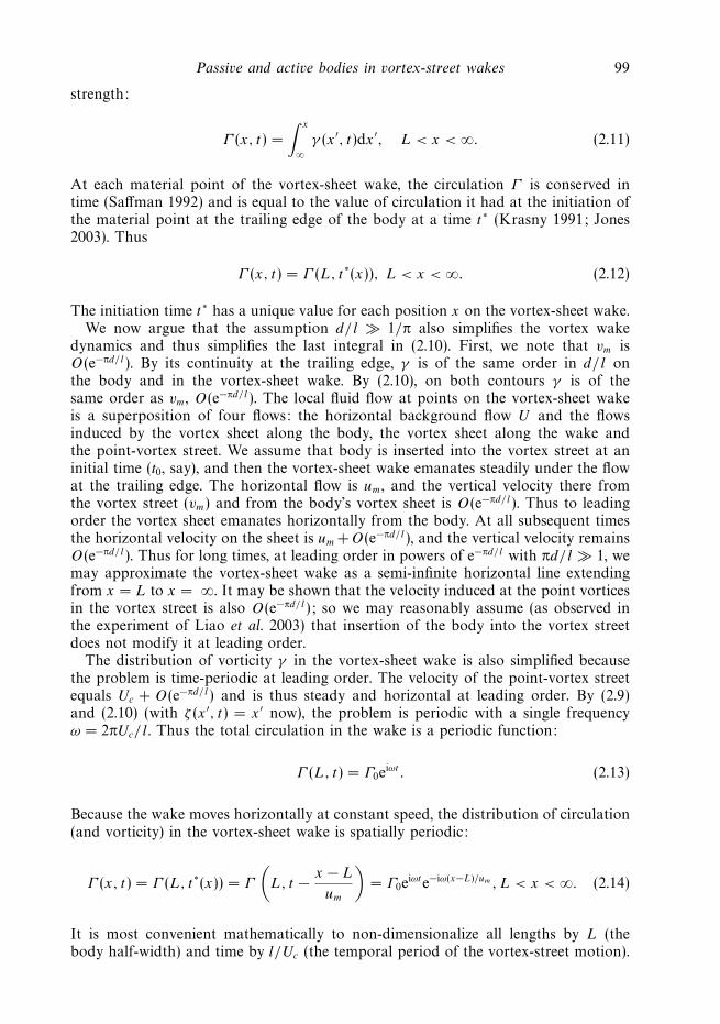
We have seen that the characteristic of the swimming shape which increases itsoutput power is the correlation between the negative of its slope and the pressurejump; the characteristic which decreases input power is the correlation between thenegative of the transverse velocity and the pressure jump. In figure 11 we plot thebody motions corresponding to the optimal phases for efficiency, again at the values


log10 k φH

log

10 l/

L

(a)

0 0.5–0.5

0

–2

2

4lo

g10 l/

L

(c)

(b)

(d)

0

–2

2

4

0–90–180 90 180

log10 k φθ

0 0.5–0.5 0–90–180 90 180

Figure 10. Contour plots of the optimal-efficiency phases for (a, b) the driving amplitude H0

and (c, d ) the pitching angle Θ0. The phase with zero phase centred on the body’s trailing edgeis shown in (a) and (c). The variation of phase along vertical lines in (a) and (c) is shown in(b) and (d ). The dotted lines give the phases for the dotted regions in (a) and (c); the solidlines give the phases in the remaining regions.

l/L = 1 and l/L = 103 and at the two wavenumbers k = 0.8 and k = 1.7. For smalll/L, the traces of the trailing edges show that the shapes are approximately ±90◦

apart from those in figure 9 in phase.For k = 0.8 and l/L = 1 (first row of figure 11), heaving and pitching motions add

constructively and yield a body motion which is delayed in phase by 90◦ from thatin the first row of figure 9. The body is still sloped upward in the first frame, whenthere is a suction force on its upper face yielding thrust. Because of the phase shiftfrom figure 9, its velocity is also upward in the first frame; so it extracts energy fromthe upward suction force. When the pressure force has changed sign 90◦ later in theperiod, the body is now moving downward with large velocity. Hence it obtains thrustand extracts energy from the vortex street. For k = 1.7 (second row of figure 11) thebody deflection and slope are nearly the opposite of those in the first row near thetrailing edge but nearly the same near the leading edge. Because the pressure forcesare largest near the leading edge, the leading edge determines the motion. At largel/L, the output power dominates the input power in the efficiency (3.44); so the thirdand fourth rows of figure 11 are essentially the same as in figure 9. As before, thesemotions correspond to a reverse von Karman street, with Γ/lU = 0.1. For a regularvon Karman street, the motions should be inverted about the centreline.

120 S. Alben

(a) (b) (c)

(d) (e) (f)

(g) (h) (i)

(j) (k) (l)

Figure 11. Motions of the body when the leading edge is driven with heaving and pitching atthe optimal phases for efficiency, as given in figures 10(b) and 10(d ). Two different wavenumbersand two difference vortex street spacings are shown. The motions when l/L = 1, small enoughfor the phases in figure 10 to have nearly converged in the long-body limit, are shown in(a)–(f ). The motions in the limit of large l/L are shown in (g)–(l ). The first column gives themotions when the optimal heaving phase is applied (without pitching). The second columngives the motions when the optimal pitching phase is applied (without heaving). The thirdcolumn superposes motions from the first two columns, with the same relative amplitudes asin the first two columns. Here we assume a reverse von Karman street, Γ/lU = 0.1.

4. Body driven along its lengthWe now apply (3.21) to a body with motion prescribed everywhere along its length.

In general the optimization problem will not have a solution unless constraints areapplied to enforce a given amplitude or smoothness of the motion (Sparenberg 1995).

We first consider the body motion which maximizes average thrust for a given(small) mean amplitude. Fixing the time-averaged amplitude of deflection to be A,the Lagrangian and its variation are

L = −〈Fx〉 − λ

(1

4

∫ 1

−1

|H |2dx − A2

), (4.1)

δL =1

2

∫ 1

−1

(−PRδH ′R − PIδH

′I − λ(HRδHR + HIδHI ))dx, (4.2)

δL = −1

2(PRδHR + PIδHI )

∣∣∣1−1

+1

2

∫ 1

−1

((P ′R − λHR)δHR + (P ′

I − λHI )δHI ) dx.

(4.3)


The solution to the variational equation is

H = AP ′/ (

1

2

∫ 1

−1

|P ′|2dx

)1/2

. (4.4)

Because P behaves like an inverse square root of distance from the leading edge anda square root of distance from the trailing edge, the integral in the denominator of(4.4) is divergent at both endpoints.

A simple alternative constraint is to fix the mean square of the slope, which meansreplacing H in (4.1) by H ′. Fixing the mean-square slope also bounds the maximumdisplacement |H | (since displacement is the integral of the slope). The Lagrangianbecomes

L1 = −〈Fx〉 − λ

(1

4

∫ 1

−1

|H ′|2dx − A21

), (4.5)

δL1 =1

2

∫ 1

−1

(−PRδH ′R − PIδH

′I − λ(H ′

RδH ′R + H ′

I δH′I )) dx, (4.6)

δL1 = −1

2((PR + λH ′

R)δHR + (PI + λH ′I )δHI )

∣∣∣1−1

+1

2

∫ 1

−1

((P ′R + λH ′′

R)δHR + (P ′I + λH ′′

I )δHI ) dx. (4.7)

Before stating the solution we note that it is also possible to constrain the mean-square curvature, which is related to the internal viscous damping in the body (suchas that due to internal connective tissue (Cheng, Pedley & Altringham 1998; Alben2009).

The minimizer of L1 is

HA1 = −1

λ

∫ x

−1

P (x) + c1x + c0, (4.8)

where c1 and c0 are constants set by the free boundary conditions on H , given bysetting the coefficients of boundary terms in (4.7) to zero. These conditions implyc1 = 0. The constant c0 does not affect L1, so it is arbitrary. We set it by setting theaverage of H1 equal to zero, consistent with small displacements. The solution H1

then becomes

HA1 = −A1

(∫ x

−1

P − 1

2

∫ 1

−1

dx

∫ x

−1

Pdx ′)/ (

1

4

∫ 1

−1

|P |2dx

)1/2

. (4.9)

The average thrust force corresponding to HA1 is

−〈Fx〉 = −1

2

∫ 1

−1

Re(P (x)H ′A1(x))dx = 2A1. (4.10)

If HA1(x) + f (x) is another body motion which has mean-square slope equal to A1,i.e.

1

4

∫ 1

−1

|H ′A1 + f ′|2dx = A2

1, (4.11)

122 S. Alben

(a) (b)

(c) (d)

Figure 12. (a, c) Swimming shapes which optimize thrust (4.9) or (b, d ) efficiency (4.15), forfixed mean slope. Here (a, b) l/L=0.4 or (c, d ) l/L = 103.

then the average thrust force is

−〈Fx〉 = −1

2

∫ 1

−1

Re(P (x)(H ′A1 +f ′))dx = 2A1 −

(14

∫ 1

−1|P |2dx

)1/2

4A1

∫ 1

−1

|f ′|2dx, (4.12)

which is clearly less than 2A1 for non-zero f . The final expression in (4.12) followsby substituting a term proportional to H ′

A1 for P in the middle expression, using (4.9)and the slope constraint (4.11).

The Lagrangian corresponding to (4.6) for maximum efficiency is given by

L1e =1

2

∫ 1

−1

Re

(P

(−1

1 + Γ/2lU

l

L∂xH − 2πiH

))dx − λ

(1

4

∫ 1

−1

|H ′|2dx − A21

),

(4.13)

δL1e =1

2

((−1

1 + Γ/2lU

l

LPR − λ

2H ′

R

)δHR +

(−1

1 + Γ/2lU

l

LPI − λ

2H ′

I

)δHI

) ∣∣∣1−1

− 1

2

∫ 1

−1

((−1

1 + Γ/2lU

l

LP ′

R − λ

2H ′′

R + 2πPI

)δHR

+

(−1

1 + Γ/2lU

l

LP ′

I − λ

2H ′′

I − 2πPR

)δHI

)dx. (4.14)

The solution is

λ

2H = −

∫ x

−1

1

1 + Γ/2lU

l

LPdx ′ − 2πi

∫ x

−1

∫ x′

−1

Pdx ′′dx ′ + c0, (4.15)

where constant λ is set so that H has mean-square slope equal to A1. The free constantc0 can be chosen to decrease the input power without affecting the constraint. Anadditional constraint is thus required to fix c0. Perhaps the simplest constraint is thesame as was used for HA1 (4.9), which is to make the mean displacement of the bodyzero. We thus focus attention on the particular shape the body assumes but not itsmean heaving motion.

In figure 12 we plot optimal swimming shapes for l/L = 0.4 and 103, values inthe asymptotic regimes of § 3.4. For small l/L, the optimal thrust shape (figure 12a)


agrees well with those in the first row of figure 9. There is an additional curvaturenear the leading edge here, due to the large pressure there. The optimal-efficiencyshape (figure 12b) resembles those in the first row of figure 11, in terms of the phaseof the trailing-edge motion relative to the vortices; it is closest in wavenumber tothese slightly flexed plates. Again, a larger slope is seen at the leading edge to takeadvantage of the larger pressure there. For larger l/L, the optimal thrust motion(figure 12c) has a slope similar to those in figures 9 and 11, but here there is no netheaving motion. The shapes now have large curvatures to take advantage of largethrust near the leading edge.

5. ConclusionWe have studied optimal swimming of a finite body in a vortex street in the limit

of small body motions, where the linearized theory is valid. In § 2 we have computedthe distribution of vorticity and pressure in the flow with respect to the strength ofthe vortex street relative to the background flow (Γ/lU ) and the streamwise spacingof the vortices relative to the body half-length (l/L). The vorticity on the body issinusoidal away from the body ends for a long body (l/L � 1) and is roughly linearaway from the ends for a short body, when the body is between vortices, and nearlyzero when the body coincides with a vortex in streamwise position. The pressureloading on the body is also oscillatory away from the ends for l/L � 1 and is nearlyproportional to the bound vorticity for l/L � 1.

We have studied two models for the body. In the first (§ 3), the body is clampedor oscillated at the leading edge. The input and output forces are computed withrespect to body mass R1 and flexibility R2. The clamped body models a passive elasticbody (such as a flapping flag) in a vortex wake. The vortices cause thrust at thelowest wavenumber mode and alternating thrust and drag in higher modes. Thesebody motions may be linearly superposed with the flag in a uniform stream to obtainthe effect of the vortex street for the fully coupled problem. The body driven at theleading edge is a model for the tail fin of a swimming fish. We identify optimal phasesfor heaving and pitching motions of the body which have clear limiting values atsmall l/L and large l/L, when phase is measured with respect to the alignment of thetrailing edge with an upper vortex. For short bodies maximizing thrust or efficiency,we find deflections away from oncoming vortices in a reverse von Karman street andtowards oncoming vortices in a regular von Karman street. For long bodies, optimalmotions at the trailing edge are phase-shifted from those for a short body by 45◦

when thrust is maximized and by 135◦ when efficiency is maximized. Optimal phasesfor intermediate lengths interpolate these values smoothly.

In the second model for the body (§ 4), its motion is prescribed along its length. Weidentify optimal swimming motions for maximum thrust and efficiency, subject to aconstraint of fixed mean body slope. We find shapes which are similar to the lowestwavenumber shapes driven at the leading edge, but with an additional upward slopenear the leading edge. This indicates that a body driven only at one end may obtaina performance nearly as good as a body driven all along its length. In applicationsto fish swimming, this supports the more frequent utilization of tail-fin swimming(carangiform and sub-carangiform) over whole-body (anguilliform) swimming, forwhich internal viscous energy losses are larger (Lighthill 1969).

Liao et al. (2003) observed trout slaloming around the vortices of an oncomingvon Karman street in their experiment. The leading edge of the trout body ledthe passage of vortices by approximately 100◦ in phase (on average), while for the

124 S. Alben

trailing edge the phase was 240◦ and for the midpoint 180◦. Also, muscle activity wasconcentrated near the leading edge of the body, similar to the model of a body drivenpassively at the leading edge in § 3. In the present work, the model most similar tothis situation is the body driven all along its length (§ 4). In the model, the pressureforces near the leading edge is dominant, and the motion of the leading edge is closein phase (ranging from 80◦ to 100◦) to that observed by Liao and Lauder, for boththe optimum thrust and optimum efficiency shapes and l/L of order 1. The phase atthe trailing edge varies over a wider range in the model. By contrast, the heaving andpitching rigid aerofoil studied by Streitlien and Triantafyllou (Streitlien et al. 1996)generally showed larger lift and thrust when the leading edge of the aerofoil movedat nearly zero phase relative to the oncoming vortex street. The reason may be thatat large heaving amplitudes, the aerofoil can be sensitive to the singular velocity nearthe point vortex.

This work was supported by the National Science Foundation Division ofMathematics Sciences, grant NSF-DMS-0810602.

Appendix. Constants in driven (or clamped) fin solutionThe constants C1, C2, C3, C4 in (3.10) are

C1 = − e−k

4k3

I2D1 − I1D2 + k2e2kD3Θ0 − k3e2kD4H0

F1

, (A 1)

C2 =ek

4k3

k2D1Θ0 + k3H0D2 + e2kD3I2 + e2kD4I1

F1

, (A 2)

C3 =1

2k3

(−I2 + k2Θ0) cosh k + (I1 + k3H0) sinh k

F2

, (A 3)

C4 =1

2k3

(I2 + k2Θ0) sinh k + (−I1 + k3H0) cosh k

F3

, (A 4)

D1 = e2k + sin(2k) + cos(2k), (A 5)

D2 = e2k − sin(2k) + cos(2k), (A 6)

D3 = e−2k − sin(2k) + cos(2k), (A 7)

D4 = e−2k + sin(2k) + cos(2k), (A 8)

F1 = 1 + cosh(2k) cos(2k), (A 9)

F2 = cosh(k) cos(k) − sinh(k) sin(k), (A 10)

F3 = cosh(k) cos(k) + sinh(k) sin(k), (A 11)

I1 = − 1

2R2

[e−k

2

∫ 1

−1

ekx′P (x ′)dx ′ − ek

2

∫ 1

−1

e−kx′P (x ′)dx ′ (A 12)

+ cos(k)

∫ 1

−1

sin(kx ′)P (x ′)dx ′ − sin(k)

∫ 1

−1


, (A 13)

I2 = − 1

2R2

[−e−k

2

∫ 1

−1

ekx′P (x ′)dx ′ − ek

2

∫ 1

−1

e−kx′P (x ′)dx ′ (A 14)

− sin(k)

∫ 1

−1

sin(kx ′)P (x ′)dx ′ − cos(k)

∫ 1

−1


. (A 15)


REFERENCES

Abrahams, M. V. & Colgan, P. W. 1987 Fish schools and their hydrodynamic function: a reanalysis.Environ. Biol. Fishes 20 (1), 79–80.

Alben, S. 2008a Optimal flexibility of a flapping appendage at high Reynolds number. J. FluidMech. 614, 355–380.

Alben, S. 2008b The flapping-flag instability as a nonlinear eigenvalue problem. Phys. Fluids 20,104–106.

Alben, S. 2009 On the swimming of a flexible body in a vortex street. J. Fluid Mech. 635, 27–45.

Alben, S., Madden, P. G. & Lauder, G. V. 2007 The mechanics of active fin-shape control inray-finned fishes. J. R. Soc. Interface 4 (13), 243–256.

Alben, S., Shelley, M. & Zhang, J. 2004 How flexibility induces streamlining in a two-dimensionalflow. Phys. Fluids 16, 1694.

Ambrose, D. M. & Wilkening, J. 2008 Global paths of time-periodic solutions of the Benjamin–Onoequation connecting arbitrary travelling waves. Preprint. ArXiv:0811.4205.

Bainbridge, R. 1963 Caudal fin and body movement in the propulsion of some fish. J. Exp. Biol.40 (1), 23–56.

Barrett, D. S., Triantafyllou, M. S., Yue, D. K. P., Grosenbaugh, M. A. & Wolfgang, M. J.

1999 Drag reduction in fish-like locomotion. J. Fluid Mech. 392, 183–212.

Batchelor, G. K. 1967 An Introduction to Fluid Dynamics . Cambridge University Press.

Bisplinghoff, R. L. & Ashley, H. 2002 Principles of Aeroelasticity . Dover.

Cheng, J.-Y., Pedley, T. J. & Altringham, J. D. 1998 A continuous dynamic beam model forswimming fish. Phil. Trans. R. Soc. Lond B 353, 981–997.

Drucker, E. G. & Lauder, G. V. 2001 Locomotor function of the dorsal fin in teleost fishes:experimental analysis of wake forces in sunfish. J. Exp. Biol. 204 (17), 2943–2958.

Drucker, E. G. & Lauder, G. V. 2005 Locomotor function of the dorsal fin in rainbow trout:kinematic patterns and hydrodynamic forces. J. Exp. Biol. 208 (23), 4479–4494.

Eloy, C., Lagrange, R., Souilliez, C. & Schouveiler, L. 2008 Aeroelastic instability of cantileveredflexible plates in uniform flow. J. Fluid Mech. 611, 97–106.

Hou, T. Y., Lowengrub, J. S. & Shelley, M. J. 2001 Boundary integrals methods formulticomponent fluids and multiphase materials. J. Comput. Phys. 169, 302–362.

Jones, M. 2003 The separated flow of an inviscid fluid around a moving flat plate. J. Fluid Mech.496, 405–441.

Krasny, R. 1991 Vortex sheet computations: roll-up, wakes, separation. Lect. Appl. Math. 28,385–402.

Liao, J. C., Beal, D. N., Lauder, G. V. & Triantafyllou, M. S. 2003 Fish exploiting vorticesdecrease muscle activity. Science 302 (5650), 1566–1569.

Lighthill, J. M. 1969 Hydromechanics of aquatic animal propulsion. Annu. Rev. Fluid Mech. 1,413–446.

Lissaman, PBS & Shollenberger, C. A. 1970 Formation flight of birds. Science 168 (3934),1003–1005.

Ristroph, L. & Zhang, J. 2008 Anomalous hydrodynamic drafting of interacting flapping flags.Phys. Rev. Lett. 101 (19), 194502.

Saffman, P. 1992 Vortex Dynamics . Cambridge University Press.

Shelley, M., Vandenberghe, N. & Zhang, J. 2005 Heavy flags undergo spontaneous oscillationsin flowing water. Phys. Rev. Lett 94, 094302.

Sparenberg, J. A. 1995 Hydrodynamic Propulsion and Its Optimization: Analytic Theory . Springer.

Streitlien, K., Triantafyllou, G. S. & Triantafyllou, M. S. 1996 Efficient foil propulsion throughvortex control. AIAA J. 34 (11), 2315–2319.

Thwaites, B. 1987 Incompressible Aerodynamics: An Account of the Theory and Observation of theSteady Flow of Incompressible Fluid Past Aerofoils, Wings and Other Bodies . Dover.

Weihs, D. 1973 Hydromechanics of fish schooling. Nature 241 (5387), 290–291.

Weimerskirch, H., Martin, J., Clerquin, Y., Alexandre, P. & Jiraskova, S. 2001 Energy savingin flight formation. Nature 413 (6857), 697–698.

Wu, T. Y. 1971 Hydromechanics of swimming propulsion. Part 1. Swimming of a two-dimensionalflexible plate at variable forward speeds in an inviscid fluid. J. Fluid Mech. 46 (2), 337–355.

Wu, T. Y. & Chwang, A. T. 1975 Extraction of flow energy by fish and birds in a wavy stream.In Swimming and Flying in Nature (ed. T. Y.-T. Wu, C. J. Brokaw & C. Brennen), vol. 2,pp. 687–702. Plenum.

Date post:	03-Dec-2016
Category:	Documents
Upload:	silas
View:	212 times
Download:	0 times

Passive and active bodies in vortex-street wakes

Documents