Patrick Breheny December 2 - University of...

Local regressionMultidimensional splines

Additive models

Multiple regression and additive models

Patrick Breheny

December 2

Patrick Breheny STA 621: Nonparametric Statistics


Additive models

Introduction

Thus far, we have discussed nonparametric regressioninvolving a single covariate

In practice, we often have a p-dimensional vector of covariatesfor each observation

The nonparametric multiple regression problem is therefore toestimate

E(y|x) = f(x)

where f : Rp 7→ R



Additive models

Local regression

We have already seen how to extend local regression to themultivariate case, back when we discussed estimatingmultivariate densities

All that is required is to define a multivariate kernel:

f(x0) =1

n

∑i

p∏j=1

1

hjK

(xij − x0j

hj

)With the kernel defined, we can now fit a weighted multipleregression model, with elements xij − x0j



Additive models

Tensor product splines

Splines can be defined in higher dimensions as well

One approach to constructing multidimensional splines isusing the tensor product basis

Suppose we specify a set of basis functions {h1k} for x1 and{h2k} for x2, with M1 and M2 elements, respectively

The tensor product basis for the two-dimensional smoothfunction of x1 and x2 is given by

gjk(x1, x2) = h1j(x1)h2k(x2)

and has M1×M2 elements



Additive models

Thin plate splines

The multidimensional analog of smoothing splines are calledthin plate regression splines

For two dimensions, we find f(x1, x2) that minimizes

−n∑

i=1

`{yi, f(x1i, x2i)}+λ∫ ∫ [

∂2f

∂u2

]2+2

[∂2f

∂u∂v

]2+

[∂2f

∂v2

]2dudv

Thin plate regression splines have fairly complicated basisfunctions



Additive models

2D smoothing

20 30 40 50 60

24

68

1012

14

m1

m2

Local regression (deg=2)

20 30 40 50 60

24

68

1012

14

Thin−plate spline

age

ldl

0.1

0.2

0.3

0.4

0.5

0.6

0.7

0.8



Additive models

2D smoothing – local linear model

20 30 40 50 60

24

68

1012

14

m1

m2

Local regression (deg=1)

20 30 40 50 60

24

68

1012

14

Thin−plate spline

age

ldl

0.1

0.2

0.3

0.4

0.5

0.6

0.7

0.8



Additive models

The curse of dimensionality

Thin plate regression splines can be extended further intohigher dimensions, but they become rather computationallyintensive as the dimension exceeds 2

Also, as we saw with kernel density estimation, the curse ofdimensionality implies that we need an exponentiallyincreasing amount of data to maintain accuracy as p increases(this applies to both local regression and splines/penalizedregression)

Furthermore, multidimensional smooth functions are harder tovisualize and interpret

Because of this, it is often necessary/desirable to introducesome sort of structure into the model



Additive models

Structured regression

Introducing structure will certainly introduce bias if thestructure does not accurate describe reality; however, it canresult in a dramatic reduction in variance

Nonparametric multiple regression usually comes down tobalancing these goals: introducing enough structure to makethe model fit stable, but not so much structure as to bias thefit

A number of methods have been proposed in the hopes ofaccomplishing this balance, including structured kernels,varying coefficient models, and projection pursuit regression

By far the simplest and most common approach, however, isto introduce an additive structure; the resulting model iscalled an additive model



Additive models

Generalized additive models

An additive model is of the form

E(y|x) = α+ f1(x1) + f2(x2) + · · ·+ fp(xp)

By introducing a link function into linear regression, we havegeneralized linear models (GLMs)

By introducing a link function into additive models, we havegeneralized additive models (GAMs):

g{E(y|x)} = α+∑j

fj(xj)



Additive models

GAMs and the curse of dimensionality

This additive structure greatly alleviates the curse ofdimensionality:

From a spline perspective, we need only∑

pmj basis functionsinstead of

∏pmj basis functions

From a local regression perspective, it is much easier to findpoints in a one-dimensional neighborhood

As we will see, additive models are also easy to fitcomputationally



Additive models

Restrictions imposed by various models

20 30 40 50 60

24

68

1012

14

GLM

age

ldl

0.1

0.2

0.3

0.4 0.5

0.6

0.7

0.8

0.9

20 30 40 50 60

24

68

1012

14

GLM w/ interaction

age

ldl

0.1

0.2

0.3

0.4

0.5

0.6 0.7 0.8

20 30 40 50 60

24

68

1012

14

GAM

age

ldl

0.1 0.2

0.3

0.4

0.5

0.6

0.7

0.8

20 30 40 50 60

24

68

1012

14

Thin−plate

age

ldl

0.1

0.2

0.3

0.4

0.5

0.6

0.7

0.8



Additive models

The gam package

As we mentioned in a previous lecture, there are two R

packages for the implementation of GAMs: mgcv and gam

The two packages both supply a gam function with a formulainterface and are superficially very similar

However, the implementation which underlies their modelfitting is very different, and as a result, they offer differentfeatures



Additive models

Backfitting

The gam package is based on a simple algorithmic approach calledbackfitting for turning any one-dimensional regression smootherinto a method for fitting additive models

(1) Initialize: α = 1n

∑i yi, fj = 0 for all j

(2) Cycle over j until convergence:

(a) Compute yi = yi − α−∑

k 6=j fk(xik) for all i

(b) Apply the one-dimensional smoother to {xij , yi} to obtain fj(c) Set fj equal to fj − n−1

∑i fj(xij)

Note that we require∑

i fj(xij) = 0 for all j; otherwise the modelis not identifiable



Additive models

Backfitting (cont’d)

The modular nature of the backfitting algorithm makes it easyto fit very general models, such as:

Models in which some terms are fit via local polynomials andothers fit via splinesModels that mix parametric and nonparametric termsModels that include 2D smooth functions to modelnonparametric interactions of terms

Computing degrees of freedom is also a simple extension ofearlier results: letting Lj denote the smoother matrix for thejth term, the degrees of freedom of the jth term is tr(Lj)− 1



Additive models

Syntax: gam

So in the gam package, one could submit

fit <- gam(y~x1+s(x2)+lo(x3))

to fit a model in which x1 is modeled parametrically, x2 ismodeled using splines, and x3 is modeled using loess

The package also provides an anova method for testingnested models:

> fit <- gam(chd~s(age)+lo(ldl)+obesity,fam="binomial")

> fit0 <- gam(chd~s(age)+ldl+obesity,fam="binomial")

> anova(fit0,fit)

Model 1: chd ~ s(age) + ldl + obesity

Model 2: chd ~ s(age) + lo(ldl) + obesity

Resid. Df Resid. Dev Df Deviance P(>|Chi|)

1 455.00 505.34

2 451.69 504.20 3.3101 1.1364 0.8134



Additive models

The mgcv package

The syntax of gam in the mgcv package is very similar,although the mgcv package has many more features

The implementation is based not on backfitting, but rather onthe Lanczos algorithm, a way of efficiently calculatingtruncated matrix decompositions

The implementation is restricted to splines (i.e. no mixing oflocal polynomials and splines)



Additive models

Selection of λ

One key advantage of this approach is that it allows for theevaluation of the derivative of GCV with respect to λj

Thus, we can employ a Newton approach to simultaneously fitthe model and optimize over the smoothing parameters withrespect to GCV

In practice, this is a big advantage over the gam package, forwhich you must specify either λj or dfj



Additive models

Syntax: mgcv

The basic syntax of gam in the mgcv package is:

fit <- gam(chd~s(age,ldl)+s(obesity),fam="binomial")

where here, we are allowing a two-way nonparametricinteraction between age and LDL, and an additivenonparametric effect of obesity on the log odds of coronaryheart disease

One can add arguments to the s() function, but the defaultbehavior is to use a natural cubic spline/thin-plate spline basisand to automatically choose the smoothing parameter viaoptimization of the GCV or AIC objective (which thepackage calls UBRE)



Additive models

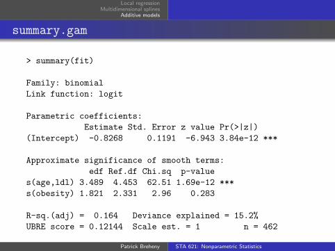
summary.gam

> summary(fit)

Family: binomial

Link function: logit

Parametric coefficients:

Estimate Std. Error z value Pr(>|z|)

(Intercept) -0.8268 0.1191 -6.943 3.84e-12 ***

Approximate significance of smooth terms:

edf Ref.df Chi.sq p-value

s(age,ldl) 3.489 4.453 62.51 1.69e-12 ***

s(obesity) 1.821 2.331 2.96 0.283

R-sq.(adj) = 0.164 Deviance explained = 15.2%

UBRE score = 0.12144 Scale est. = 1 n = 462



Additive models

anova.gam

More specific hypotheses can be tested via the anova method:

> fit0 <- gam(chd~s(age,ldl)+obesity,data=heart,family="binomial")

> anova(fit0,fit,test="Chisq")

Model 1: chd ~ s(age, ldl) + obesity

Model 2: chd ~ s(age, ldl) + s(obesity)


1 457.21 509.76

2 455.69 505.48 1.5202 4.272 0.07496 .



Additive models

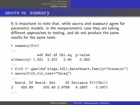
anova vs. summary

It is important to note that, while anova and summary agree forparametric models, in the nonparametric case they are takingdifferent approaches to testing, and do not produce the sameresults for the same tests:

> summary(fit)

...

edf Ref.df Chi.sq p-value

s(obesity) 1.821 2.331 2.96 0.283

...

> fit0 <- gam(chd~s(age,ldl),data=heart,family="binomial")

> anova(fit0,fit,test="Chisq")

...


2 455.69 505.48 2.9798 6.2867 0.0971

...



Additive models

anova vs. summary

This is due to two factors:

When models are refit, the optimal values of λj do not staythe same

The hypothesis test in summary attempts to adjust for thefact that λ is chosen based on the data rather than fixed; todo so, it computes a modified χ2 statistic with an inflatednumber of degrees of freedom



Additive models

Comments on hypothesis testing

It should be pointed out once again that these tests areapproximate, and should be taken as only a rough guideconcerning statistical significance

This issue is in no way unique to GAMs; any time modelselection is performed, the resulting p-value are no longer validand should be taken as only rough indicators of significance

Which type of test (anova vs. summary) is appropriatedepends on the situation and the goals of the analysis

Finally, keep in mind that hypothesis testing is often not anappropriate goal in regression modeling in the first place, andthat building a model that predicts the outcome well (asmeasured by CV /GCV /AIC) is often a more meaningfulgoal



Additive models

1D plots

plot(fit,shade=TRUE)

15 20 25 30 35 40 45

−1

01

2

obesity

s(ob

esity

,1.8

2)



Additive models

2D plots

vis.gam(fit,plot.type="contour")

20 30 40 50 60

24

68

1012

14

response

age

ldl

0.1

0.2

0.3

0.4

0.5

0.6

0.7

0.8

0.9



Additive models

Comments

Note that, although one may specify a nonparametric form,gam will often return linear or nearly linear fits for someparameters because this is the fit that optimized the GCVcriterion

For example, in the heart study, the age-LDL interaction had3.5 degrees of freedom, only slightly more flexible than the 3degrees of freedom arising from a parametric interaction

This is entirely driven by the data: as an example, I was onceworking on a project in which I found a meaningful three-wayinteraction between age, driving distance, and urban/rurallocation on the probability that an individual would attend anintervention designed to educate women aged 40-64 on livinghealthier lifestyles



Additive models

A nonparametric three-way interaction:

0 10 20 30 40

4045

5055

60

Rural

Distance

Age 0.05

0.1

0.15 0.2 0.2

0.25

0.3

0.35

0.4

0.45 0.5 0.

55

0 10 20 30 4040

4550

5560

Urban

Distance

Age

0.3

0.35

0.4

0.45

0.5

0.55


Date post:	10-Jul-2018
Category:	Documents
Upload:	lekhanh
View:	214 times
Download:	0 times

Patrick Breheny December 2 - University of...

Documents