59
Descriptive statistics Correlation Regression Descriptive statistics; Correlation and regression Patrick Breheny September 16 Patrick Breheny STA 580: Biostatistics I 1/59
Descriptive statisticsCorrelationRegression
Descriptive statistics; Correlation and regression
Patrick Breheny
September 16
Patrick Breheny STA 580: Biostatistics I 1/59
Descriptive statisticsCorrelationRegression
IntroductionHistogramsNumerical summariesPercentiles
Tables and figures
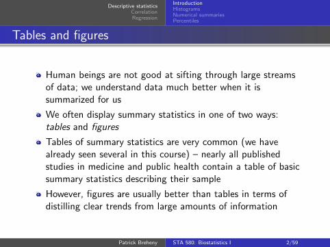
Human beings are not good at sifting through large streamsof data; we understand data much better when it issummarized for us
We often display summary statistics in one of two ways:tables and figures
Tables of summary statistics are very common (we havealready seen several in this course) – nearly all publishedstudies in medicine and public health contain a table of basicsummary statistics describing their sample
However, figures are usually better than tables in terms ofdistilling clear trends from large amounts of information
Patrick Breheny STA 580: Biostatistics I 2/59
Descriptive statisticsCorrelationRegression
IntroductionHistogramsNumerical summariesPercentiles
Types of data
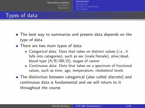
The best way to summarize and present data depends on thetype of data
There are two main types of data:
Categorical data: Data that takes on distinct values (i.e., itfalls into categories), such as sex (male/female), alive/dead,blood type (A/B/AB/O), stages of cancerContinuous data: Data that takes on a spectrum of fractionalvalues, such as time, age, temperature, cholesterol levels
The distinction between categorical (also called discrete) andcontinuous data is fundamental and we will return to itthroughout the course
Patrick Breheny STA 580: Biostatistics I 3/59

Descriptive statisticsCorrelationRegression
IntroductionHistogramsNumerical summariesPercentiles
Categorical data
Summarizing categorical data is pretty straightforward – youjust count how many times each category occurs
Instead of counts, we are often interested in percents
A percent is a special type of rate, a rate per hundred
Counts (also called frequencies), percents, and rates are thethree basic summary statistics for categorical data, and areoften displayed in tables or bar charts, as we saw in lab
Patrick Breheny STA 580: Biostatistics I 4/59

Descriptive statisticsCorrelationRegression
IntroductionHistogramsNumerical summariesPercentiles
Continuous data
For continuous data, instead of a finite number of categories,observations can take on a potentially infinite number ofvalues
Summarizing continuous data is therefore much lessstraightforward
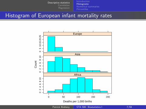
To introduce concepts for describing and summarizingcontinuous data, we will look at data on infant mortality ratesfor 111 nations on three continents: Africa, Asia, and Europe
Patrick Breheny STA 580: Biostatistics I 5/59

Descriptive statisticsCorrelationRegression
IntroductionHistogramsNumerical summariesPercentiles
Histograms
One very useful way of looking at continuous data is withhistograms
To make a histogram, we divide a continuous axis into equallyspaced intervals, then count and plot the number ofobservations that fall into each interval
This allows us to see how our data points are distributed
Patrick Breheny STA 580: Biostatistics I 6/59
Descriptive statisticsCorrelationRegression
IntroductionHistogramsNumerical summariesPercentiles
Histogram of European infant mortality rates
Deaths per 1,000 births
Cou
nt
02
46
810
0 50 100 150 200
Africa
02
46
810
Asia
05
1015
2025
Europe
Patrick Breheny STA 580: Biostatistics I 7/59

Descriptive statisticsCorrelationRegression
IntroductionHistogramsNumerical summariesPercentiles
Summarizing continuous data
As we can see, continuous data comes in a variety of shapes
Nothing can replace seeing the picture, but if we had tosummarize our data using just one or two numbers, howshould we go about doing it?
The aspect of the histogram we are usually most interested inis, “Where is its center?”
This is typically represented by the average
Patrick Breheny STA 580: Biostatistics I 8/59

Descriptive statisticsCorrelationRegression
IntroductionHistogramsNumerical summariesPercentiles
The average and the histogram
The average represents the center of mass of the histogram:
Deaths per 1,000 births
Cou
nt
02
46
810
0 50 100 150 200
Africa
02
46
810
Asia
05
1015
2025
Europe
Patrick Breheny STA 580: Biostatistics I 9/59

Descriptive statisticsCorrelationRegression
IntroductionHistogramsNumerical summariesPercentiles
Spread
The second most important bit of information from thehistogram to summarize is, “How spread out are theobservations around the center”?
This is most typically represented by the standard deviation
To understand how standard deviation works, let’s return toour small example with the numbers {4, 5, 1, 9}Each of these numbers deviates from the mean by someamount:
4− 4.75 = −0.75 5− 4.75 = 0.25
1− 4.75 = −3.75 9− 4.75 = 4.25
How should we measure the overall size of these deviations?
Patrick Breheny STA 580: Biostatistics I 10/59

Descriptive statisticsCorrelationRegression
IntroductionHistogramsNumerical summariesPercentiles
Root-mean-square
Taking their mean isn’t going to tell us anything (why not?)
We could take the average of their absolute values:
|−0.75|+ |0.25|+ |−3.75|+ |4.25|4
= 2.25
But it turns out that for a variety of reasons, theroot-mean-square works better as a measure of overall size:√
(−0.75)2 + (0.25)2 + (−3.75)2 + (4.25)2
4≈ 2.86
Patrick Breheny STA 580: Biostatistics I 11/59

Descriptive statisticsCorrelationRegression
IntroductionHistogramsNumerical summariesPercentiles
The standard deviation
The formula for the standard deviation is
s =
√∑ni=1(xi − x̄)2
n− 1
Wait a minute; why n− 1?
The reason (which we will discuss further in a few weeks) isthat dividing by n turns out to underestimate the truestandard deviation
Dividing by n− 1 instead of n corrects some of that bias
The standard deviation of {4, 5, 1, 9} is 3.30 (recall that wegot 2.86 if we divide by n)
Patrick Breheny STA 580: Biostatistics I 12/59

Descriptive statisticsCorrelationRegression
IntroductionHistogramsNumerical summariesPercentiles
Meaning of the standard deviation
The standard deviation (SD) describes how far away numbersin a list are from their average
The SD is often used as a “plus or minus” number, as in“adult women tend to be about 5’4, plus or minus 3 inches”
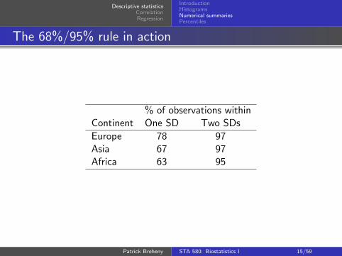
Most numbers (roughly 68%) will be within 1 SD away fromthe average
Very few entries (roughly 5%) will be more than 2 SD awayfrom the average
This rule of thumb works very well for a wide variety of data;we’ll discuss where these numbers come from in a few weeks
Patrick Breheny STA 580: Biostatistics I 13/59

Descriptive statisticsCorrelationRegression
IntroductionHistogramsNumerical summariesPercentiles
Standard deviation and the histogram
Background areas within 1 SD of the mean are shaded:
Deaths per 1,000 births
Cou
nt
02
46
810
50 100 150 200
Africa
02
46
0 50 100 150
Asia
05
1015
10 20 30 40
Europe
Patrick Breheny STA 580: Biostatistics I 14/59
Descriptive statisticsCorrelationRegression
IntroductionHistogramsNumerical summariesPercentiles
The 68%/95% rule in action
% of observations withinContinent One SD Two SDs
Europe 78 97Asia 67 97Africa 63 95
Patrick Breheny STA 580: Biostatistics I 15/59

Descriptive statisticsCorrelationRegression
IntroductionHistogramsNumerical summariesPercentiles
Summaries can be misleading!
All of the following have the same mean and standard deviation:
−4 −2 0 2 4F
requ
ency
−4 −2 0 2 4
−4 −2 0 2 4
Fre
quen
cy
−4 −2 0 2 4
Patrick Breheny STA 580: Biostatistics I 16/59

Descriptive statisticsCorrelationRegression
IntroductionHistogramsNumerical summariesPercentiles
Percentiles
The average and standard deviation are not the only ways tosummarize continuous data
Another type of summary is the percentile
A number is the 25th percentile of a list of numbers if it isbigger than 25% of the numbers in the list
The 50th percentile is given a special name: the median
The median, like the mean, can be used to answer thequestion, “Where is the center of the histogram?”
Patrick Breheny STA 580: Biostatistics I 17/59

Descriptive statisticsCorrelationRegression
IntroductionHistogramsNumerical summariesPercentiles
Median vs. mean
The dotted line is the median, the solid line is the mean:
Deaths per 1,000 births
Cou
nt
02
46
810
50 100 150 200
Africa
02
46
0 50 100 150
Asia
05
1015
10 20 30 40
Europe
Patrick Breheny STA 580: Biostatistics I 18/59
Descriptive statisticsCorrelationRegression
IntroductionHistogramsNumerical summariesPercentiles
Skew
Note that the histogram for Europe is not symmetric: the tailof the distribution extends further to the right than it does tothe left
Such distributions are called skewed
The distribution of infant mortality rates in Europe is said tobe right skewed or skewed to the right
For asymmetric/skewed data, the mean and the median willbe different
Patrick Breheny STA 580: Biostatistics I 19/59

Descriptive statisticsCorrelationRegression
IntroductionHistogramsNumerical summariesPercentiles
Hypothetical example
Azerbaijan had the highest infant mortality rate in Europe at37
What if, instead of 37, it was 200?
Mean Median
Real 14.1 11Hypothetical 19.2 11
The mean is now higher than 72% of the countries
Note that the average is sensitive to extreme values, while themedian is not; statisticians say that the median is robust tothe presence of outlying observations
Patrick Breheny STA 580: Biostatistics I 20/59
Descriptive statisticsCorrelationRegression
IntroductionHistogramsNumerical summariesPercentiles
Box plots
Quantiles are used in a type of graphical summary called abox plot
Box plots are constructed as follows:
Calculate the three quartiles (the 25th, 50th, and 75th)Draw a box bounded by the first and third quartiles and with aline in the middle for the medianCall any observation that is extremely far from the box an“outlier” and plot the observations using a special symbol (thisis somewhat arbitrary and different rules exist for definingoutliers)Draw a line from the top of the box to the highest observationthat is not an outlier; likewide for the lowest non-outlier
Patrick Breheny STA 580: Biostatistics I 21/59

Descriptive statisticsCorrelationRegression
IntroductionHistogramsNumerical summariesPercentiles
Box plots of the infant mortality rate data
●
●
●
Africa Asia Europe
050
100
150
Patrick Breheny STA 580: Biostatistics I 22/59

Descriptive statisticsCorrelationRegression
IntroductionCorrelation
Introduction
Box plots are a way to examine the relationship between acontinuous variable and a categorical variable
In lab, we saw bar charts as a way of comparing two (or more)categorical variables
Now, we will discuss how to summarize and illustrate therelationship between two continuous variables
Patrick Breheny STA 580: Biostatistics I 23/59

Descriptive statisticsCorrelationRegression
IntroductionCorrelation
Pearson’s height data
Statisticians in Victorian England were fascinated by the ideaof quantifying hereditary influences
Two of the pioneers of modern statistics, the VictorianEnglishmen Francis Galton and Karl Pearson were quitepassionate about this topic
In pursuit of this goal, they measured the heights of 1,078fathers and their (fully grown) sons
Patrick Breheny STA 580: Biostatistics I 24/59

Descriptive statisticsCorrelationRegression
IntroductionCorrelation
The scatter plot
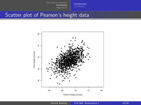
As we’ve mentioned, it is important to plot continuous data –this is especially true when you have two continuous variablesand you’re interested in the relationship between them
The most common way to plot the relationship between twocontinuous variables is the two-way scatter plot
Scatter plots are created by setting up two continuous axes,then creating a dot for every pair of observations
Patrick Breheny STA 580: Biostatistics I 25/59
Descriptive statisticsCorrelationRegression
IntroductionCorrelation
Scatter plot of Pearson’s height data
●
● ●
●
● ●●●
●
●
● ●●
● ●
●●
●
●
●●
●
●●
●●●
●
●● ●●
●
●
●●
● ● ●
●●
●●
●●
●●
●
●
●
●● ●
●● ●
●
●●
●
●● ●
●●
●●●
● ●●
●
●
●
●●● ●●
●
●●
●
●
●●●
●●
●●
●
●
●●
●
●●
●
●●
●
●
● ●
●
● ●●
●
●● ●
●●
●
● ●●●
●●
●●●
●
●
●
●●
●
● ● ●
●●●
●● ●
●
●
●●
●
●●●●
●●●
●● ●
●
● ●
●
●
●●
●●
●
●●
●●
●●
●●●
●
●●
●
●
●
●●
●
●● ●
●●●
●●
●●
●
●●
● ●
● ●●
●●
●
●
●
●
●
●
●
●
●
●
●
●
●
●
● ●
●
● ●
●
●
●●
● ●
●
●●●
● ●
●
●
●
● ●
● ●● ● ●●●
●●
●
●
●●
●
●
● ●
●●
● ●●
●
●
●
●●
● ●●
●
●
●●
●
●
●●
●●
●●
●●● ●
●
●
●●
● ● ●● ● ●
●●
●●
● ●
● ●●
●● ●
●
●●
●●
●●●
●●
●●●
●●
●
●
● ●●
●●
●
●● ● ●
●
●
● ●●●●
●
●
●●
● ●●●
● ● ●●● ●
●
●●●
●● ●
●
●●
● ●●
●
●
●● ●
●
●●
●●
●
● ●●●● ●●
●
●●
● ●
●
●
● ● ●●
●● ●
●
●●●
●●
●●●
● ●
●
●
●
●
●●
●
●
●
●
●
●
●
●
●
●
●
●
●
●
●
●●
●
●
● ●●
●
●
●
●
●
●●●
●●
● ●●
●
● ●●
●●
●●
●
●
●
●
●●● ●●
●
●●
●
●
●●
●
●
●
●
●●
●●●
●●
● ●●
●●●●●● ● ●
●●
●●
●
●
●●
●●●
●●
●● ●
●●●
●● ●
●●●
●
●●●●
●
●●
●
● ●●
●●
●
●
●●●
●●● ●●
●●●
●●●
●●●
●
●●
●
●
●
●
●
●●
●●
●
●●●
●
●
●
●
●●
●
●●
● ●
●●
●
●
●
● ● ● ●●
●●
●●
●
●
● ●●
●
●● ●
●
●
●●
●● ●
●
●●
● ●
●
●
● ●● ●
●
● ●
●
●
●●●
●
●
●
●
●
●
●●
●
●
●
●
●
●
●
●
●
● ●●
●
●
●●
●●
●
●●
●
● ●●
●●
●
●●
●
● ●● ● ●●
●●●
●●
●
● ●
● ● ●
●● ● ●
●
●
●
●
●
●● ● ●●●
● ●
● ●
●
●
●●● ●●
●●
●
●●
●●
●
●●
●● ●●● ●
●●●
●● ●
●
● ●
●
●
●●●
● ●●
●
●●● ●
● ●●
●●
●●
●●
●●
●● ●
●
● ●
● ●
●
●●● ●
●●
●
●
● ●●
●
●●
●
●●
●●●●●
● ●●
●
● ●●●● ●
●●
●
●
● ●●
●●●●
●
●
●
●
● ●●●
●
●
●● ● ●
●●
● ●
●
●●
●
●●
●
● ●
●
●
●
●●
●
●
●
●
●
●
●
●
●
●
●
●
●
●
●
●
●●
●● ● ● ●
●●
●
●
●●●
●●
●
● ●
● ●
●
●
● ●● ●●
● ●●●
●●
●●
●
●
● ●
●● ●
●●
●
●
●
●
●
●●●
●
●
●
●●●
●
●
●
●● ● ●●
● ●●
●●
●
●●
●
●
●●●● ●
●●
●●
●●●
●
●
● ●● ●●
●●●
●●
● ●●
●
●● ●
● ●●●
●
●●
●●
●●●
●●●
●●
●●
●
●●
●● ●
●
●
●●
● ●
●
●●
●
● ● ●● ●
●●●●
●
● ●● ●
●
●●●
●
●●● ●●
●●●
●●
●
●
●
●●
●
●
●●
●●
●●
●●●
● ●
●●
●
●
●●
●
● ● ● ●
●
●
●
●
●
●
●
●
●
●
●
●●
●
60 65 70 75 80
6065
7075
80
Father's height (Inches)
Son
's h
eigh
t (In
ches
)
Patrick Breheny STA 580: Biostatistics I 26/59
Descriptive statisticsCorrelationRegression
IntroductionCorrelation
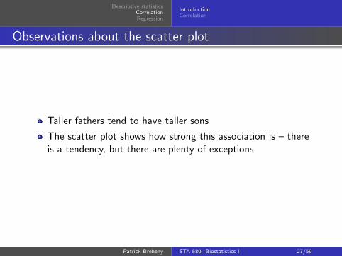
Observations about the scatter plot
Taller fathers tend to have taller sons
The scatter plot shows how strong this association is – thereis a tendency, but there are plenty of exceptions
Patrick Breheny STA 580: Biostatistics I 27/59
Descriptive statisticsCorrelationRegression
IntroductionCorrelation
Standardizing a variable
Before we summarize this relationship numerically, we mustdiscuss the idea of standardizing a variable
In Pearson’s height data, one of the sons measured 63.2inches tall
Because the average height of the sons in the sample was 68.7inches, another way of describing his height is to say that hewas 5.5 inches below average
Furthermore, because the standard deviation of the sons was2.8 inches, yet another way of describing his height is to saythat he was 1.9 standard deviations below the average
Patrick Breheny STA 580: Biostatistics I 28/59

Descriptive statisticsCorrelationRegression
IntroductionCorrelation
The standardization formula
Putting this into a formula, we standardize an observation xiby subtracting the average and dividing by the standarddeviation:
zi =xi − x̄SDx
where x̄ and SDx are the mean and standard deviation of thevariable x
One virtue of standardizing a variable is interpretability:
If someone tells you that the concentration of urea in yourblood is 50 mg/dL, that likely means nothing to youOn the other hand, if you are told that the concentration ofurea in your blood is 4 standard deviations above average, youcan immediately recognize this as a very high value
Patrick Breheny STA 580: Biostatistics I 29/59

Descriptive statisticsCorrelationRegression
IntroductionCorrelation
More benefits of standardization
If you standardize all of the observations in your sample, theresulting variable will be “standardized” in the sense of havingmean 0 and standard deviation 1
Standardization therefore brings all variables onto a commonscale – regardless of whether the heights were originallymeasured in inches, centimeters, or miles, the standardizedheights will be identical
As we will see momentarily, this allows us to study therelationship between two continuous variables withoutworrying about the scale of measurement
The concept behind standardization – taking an observation,then subtracting the expected value and dividing by thevariability – is fundamental to statistics and we will variationson this idea many times in this course
Patrick Breheny STA 580: Biostatistics I 30/59

Descriptive statisticsCorrelationRegression
IntroductionCorrelation
The correlation coefficient
The summary statistic for describing the strength ofassociation between two variables is the correlation coefficient,denoted by r (and sometimes called Pearson’s correlationcoefficient)
The correlation coefficient is always between 1 (perfectpositive correlation) and -1 (perfect negative correlation), andcan take on any value in between
A positive correlation means that as one variable increases,the other one tends to increase as well
A negative correlation means that as one variable increases,the other one tends to decrease
Patrick Breheny STA 580: Biostatistics I 31/59
Descriptive statisticsCorrelationRegression
IntroductionCorrelation
Calculating the correlation coefficient
The correlation coefficient is simply the average of theproducts of the standardized variables
In mathematical notation,
r =
∑ni=1 z
xi z
yi
n− 1,
where zxi and zyi are the standardized values of x and y
Note: The “n versus n− 1” issue has nothing to do withcorrelation; however, if n− 1 is used when standardizing, itmust be used again here
Patrick Breheny STA 580: Biostatistics I 32/59

Descriptive statisticsCorrelationRegression
IntroductionCorrelation
Meaning behind the correlation coefficient formula
●
● ●
●
● ●●●
●
●
● ●●
● ●
●●
●
●
●●
●
●●
●●●
●
●● ●●
●
●
●●
● ● ●
●●
●●
●●
●●
●
●
●
●● ●
●● ●
●
●●
●
●● ●
●●
●●●
● ●●
●
●
●
●●● ●●
●
●●
●
●
●●●
●●
●●
●
●
●●
●
●●
●
●●
●
●
● ●
●
● ●●
●
●● ●
●●
●
● ●●●
●●
●●●
●
●
●
●●
●
● ● ●
●●●
●● ●
●
●
●●
●
●●●●
●●●
●● ●
●
● ●
●
●
●●
●●
●
●●
●●
●●
●●●
●
●●
●
●
●
●●
●
●● ●
●●●
●●
●●
●
●●
● ●
● ●●
●●
●
●
●
●
●
●
●
●
●
●
●
●
●
●
● ●
●
● ●
●
●
●●
● ●
●
●●●
● ●
●
●
●
● ●
● ●● ● ●●●
●●
●
●
●●
●
●
● ●
●●
● ●●
●
●
●
●●
● ●●
●
●
●●
●
●
●●
●●
●●
●●● ●
●
●
●●
● ● ●● ● ●
●●
●●
● ●
● ●●
●● ●
●
●●
●●
●●●
●●
●●●
●●
●
●
● ●●
●●
●
●● ● ●
●
●
● ●●●●
●
●
●●
● ●●●
● ● ●●● ●
●
●●●
●● ●
●
●●
● ●●
●
●
●● ●
●
●●
●●
●
● ●●●● ●●
●
●●
● ●
●
●
● ● ●●
●● ●
●
●●●
●●
●●●
● ●
●
●
●
●
●●
●
●
●
●
●
●
●
●
●
●
●
●
●
●
●
●●
●
●
● ●●
●
●
●
●
●
●●●
●●
● ●●
●
● ●●
●●
●●
●
●
●
●
●●● ●●
●
●●
●
●
●●
●
●
●
●
●●
●●●
●●
● ●●
●●●●●● ● ●
●●
●●
●
●
●●
●●●
●●
●● ●
●●●
●● ●
●●●
●
●●●●
●
●●
●
● ●●
●●
●
●
●●●
●●● ●●
●●●
●●●
●●●
●
●●
●
●
●
●
●
●●
●●
●
●●●
●
●
●
●
●●
●
●●
● ●
●●
●
●
●
● ● ● ●●
●●
●●
●
●
● ●●
●
●● ●
●
●
●●
●● ●
●
●●
● ●
●
●
● ●● ●
●
● ●
●
●
●●●
●
●
●
●
●
●
●●
●
●
●
●
●
●
●
●
●
● ●●
●
●
●●
●●
●
●●
●
● ●●
●●
●
●●
●
● ●● ● ●●
●●●
●●
●
● ●
● ● ●
●● ● ●
●
●
●
●
●
●● ● ●●●
● ●
● ●
●
●
●●● ●●
●●
●
●●
●●
●
●●
●● ●●● ●
●●●
●● ●
●
● ●
●
●
●●●
● ●●
●
●●● ●
● ●●
●●
●●
●●
●●
●● ●
●
● ●
● ●
●
●●● ●
●●
●
●
● ●●
●
●●
●
●●
●●●●●
● ●●
●
● ●●●● ●
●●
●
●
● ●●
●●●●
●
●
●
●
● ●●●
●
●
●● ● ●
●●
● ●
●
●●
●
●●
●
● ●
●
●
●
●●
●
●
●
●
●
●
●
●
●
●
●
●
●
●
●
●
●●
●● ● ● ●
●●
●
●
●●●
●●
●
● ●
● ●
●
●
● ●● ●●
● ●●●
●●
●●
●
●
● ●
●● ●
●●
●
●
●
●
●
●●●
●
●
●
●●●
●
●
●
●● ● ●●
● ●●
●●
●
●●
●
●
●●●● ●
●●
●●
●●●
●
●
● ●● ●●
●●●
●●
● ●●
●
●● ●
● ●●●
●
●●
●●
●●●
●●●
●●
●●
●
●●
●● ●
●
●
●●
● ●
●
●●
●
● ● ●● ●
●●●●
●
● ●● ●
●
●●●
●
●●● ●●
●●●
●●
●
●
●
●●
●
●
●●
●●
●●
●●●
● ●
●●
●
●
●●
●
● ● ● ●
●
●
●
●
●
●
●
●
●
●
●
●●
●
60 65 70 75 80
6065
7075
80
Father's height (Inches)
Son
's h
eigh
t (In
ches
)
For this data, r = .50 Patrick Breheny STA 580: Biostatistics I 33/59
Descriptive statisticsCorrelationRegression
IntroductionCorrelation
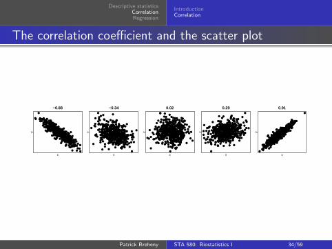
The correlation coefficient and the scatter plot
●
●
●
●
●
●
●
●
●
●●
●
●
●
●
●
●●●
●
●
●
●
●
●●
●
●
●
●
●
●
●
●
●
●
●
●
●
●●
●
●
●
●
●
● ●
●
●
●
●
● ●
●●
●
●
●●
●●
●●
●
●
●
●
● ●
●
●
●
● ●
●
●
●
●
●
●
●
●
● ●
●
● ●
●
●
●
●
●
●
●
●
●
●
●
●
●
●
●
●
●
●
●
●
●
●●
●●
●
●
● ●
●
●
●
●
●
●
●
●
●
●
●
●
●●
●
●
●
●
●
●
●
●
●
●
●
●
●●●
●
●
●
●
●
●
●
●
●
●
●
●
●●
●
●
●
●
●
●
●
●
●
●
● ●
●●
●
●●
●
●
●
●●
●
●
●
●
●
●
●
●
●●
●
● ●
●
●
●
●
●
●
● ●●
●
●
● ● ●
●
●
●
●●
●
●
●
●
● ●●
●
●
●
●
●
●
●
●●
●
●●
●
●●
●
●
●
●
●●
●
●●
●
●
● ●
●
●
●●
●
●
●●
●●
●
●●●
●
●
●
● ●
●●●
●
●
●
●
●
●
●●
●
●
●
●
●●
●
● ●
●
●
●
●
●
● ●
●
●
●
●●
●●
●●
●
●●
●●
●
●
●
●●
●
●
●
●
●
●
●
●
●
●
●●
●
●●
●
●●
●
●
●
●●
●
●
●
●
●
●
●
●
●
●
●
●
●● ●
●●●●
●
●
●
●
●●
●
●
●●●
●
●
●●
●
●
●
●●
●
●
●
●
●
● ●
●●●
●
●
●
●●
●
●
●
●
●
● ●
●●
●
●
●●●
● ●
●
●●
●●
●
●
●
●
●
●
●
●
●
●
●
●
●
●
●
●
●
●
●
●
●
●●
●
●
●●
●
●
●
● ●●
●●
●
●
●
●
●
●●
●
●
●
●
●
●
●
●
●
●
●
●
●
●
●
●
●
●●
●
●
●●
●
●
●
●
●
●
●●
●
●
●
●
●
●●●
●
●
●
●
●
●
●
−0.88
y
x
●
●
●
●
●
●
●
●
●●
●
●
●
● ●
●
●●
●●
●●
●
●
●
●
●
●
●
●
●●
●●
●
●●
●
●●
●
●
●●
●
●
●
●●
●
●
●
●
●●
●
●
●●●
●
●
●
●● ●
●
●
●
●
●
●
●
●
●
●
● ●
●
●
●
●
●●
●●
●
●
●
●
●
●● ●●
●
●
●
●
●
●
●
●
●
●
●
●
●
●
●
●
●
●
● ●
●●
●
●
●
●
●
●
●
●
●
●
●
●
●
●
●
●
●
●
●
●●
●●
●
●●
●
●
●●
●
●
●●
●●
●
●
●
●●
●
●
●
●
●●
●
●●
●
●
●
●
●
●
●
●
●●
● ●●
●
●
●
●
●
●
●
●
●
●
●
●
●●
●
●
●
●
●●
●
●●●
●
●
● ●
●●
●●
●
●
●
●●
● ●
●
●
●
●
●●
●
●
●
●
●
●●
●
●
●
●
●
●
●
●
●
● ●●
●●
●
●
●
● ●
●
●
●
●
●
●
●●
●
●
●
●●●
●
●
●
●
●
●
●●
●
●
●
●
●
●
●
●
●●●
●
●
●
●
●
●
●
●
●
●●
●
●●
●●● ●
●
●
●
●
●
●
●
●
●●
●
●
●
●
●
●
●
●
●
●
●●
●
●
●
●●
●
●
●
●
●
●
●
●
●
●
●
●
●
●
●●●
●
●
●
●
●
●
●
●
●
●
●
●
●
● ●
●
●
●
●
●
●
●
●
●●
●
●
●● ●●
●
●
●
●
●
●
●
●
● ●
●
●
●
●
●
●
●
●
●●
●
●
●
●
●● ●
●
●
●
●
●●
●
●
●
●
●
●
●
●
●
●
●●
●●
●
●
●
●
● ●
●
●●●
●●
●●
●
●
●●
●●
●●
●
●
●
●
●●
●
●●
●
● ●
●
●
●●
●
●
●
●
●
●●
●
●
●●
●
●●
●
●
●●
●
●
●
●
●
●
●
●
●●
●
●
●●
●
●
●
● ●
●
−0.34
y
x
●
●
●
●
●
●
●
●
●
●
●●●
●●
●●
●
●
●
●
●
●
●
●●
●
●
●●
●
●
●
●
●
●
●
●
●
●
●
●
●●
●
●
●● ●
●●
●
●
●
●
●
●●
●●
●
● ●●● ●
●●
●
●●
●
●
●
●
●
●
●
●
●
●
●
●●
●
●
●
●
●
●
● ●
●
●
●
●
●
●
● ●
●
●
●
●
●
●
●
●
●
●
●
●
●
●
●●
●
●
●
●
● ●
●●
●
●
●
●
●
●
●●
●
●●
●
●
●
●
●
●
●
●
●
●●
●
●
●
●
●● ●
●
●
●
●
●
●
●
●
●●
●
●
●●
●●
●
●
●
●●
●
●
●
●
●
●
●
●● ●●●
●
●●
●
●
●
●
●●
●
●
●●
●●
●
●
●
●
●
●
●
●
●
●
●
●
●
●
●●
●
●●
●●
●
●
●
●
●
●
●
●
●●
●
●
●●
●
●
● ●
●
●
●
●
●
●●
●●
●●
●
●
●
●
●
●
●
●
●
●
●
●
●●
●
●
●
●
● ●●
●
●
●
●
●
●
●●
●
●
●
●
●
●
●
●
●
●
●
●
●●
●
●
●
● ●
●
●
●●
●
●
● ●
●
●
●
●
●
● ●
●
●
●
●
●●
●
●●
●
●
●
●
●
●
●
●
●
●
●
●
●
●
●
●
●
●
●
●
●
●
●
●
●
●
●●
●●● ●
●
●
●●●
●
●
●●
●
●●
●
●
●
●
●
●
●
●●
●
●
●
●●
●
●
●
●
●
●
●
●
●
●
●●
●
●
●
●
●
●
●
●
●
●
●
●
●
●
● ●
●●
●●
●
●
●
●
●
●
●
●
●
●
●●
●
●
●
●
●
●
●
●
●
●
●
●
●
●
●
●
●
●
●
●
●
●
●
●
●
●
●
●
●
●●
●
●●
●
●
●
●
●●
●
●●
●
●●
●
●●
●
●●
●
●
●
●
●
●
●
●
●
●●
●● ●
●
●
●
● ●
●
●● ●
0.02
y
x
●
●
●
●
●
●
●
●
●
●●
●
●
●
●
●
●
●●
●
●
●
●
●
●
●
●
●
●●
●
●
●
● ●
●
●
●
●
●
●
●
●
●
●
●
●
●
●
●
●
●
●
●
●
●
● ●
●
●●
●
●
●●
●
●
●
●
●
●
●
●
●
●
●
●
●
● ●
●
●
●
●
●
●●
● ●
●
●●
●
●
●
●
●
●
●
●
●
●
● ●
●
●
●
●
●
●
●
●
●
●●
●
●
●
●
●●
●●
●
●
●
●
● ●
●●
●●
●●
●●
●
●
●
●●
●
●
●●
●
●
●
●
●
●●
●●
●
●
●
●
●
●
●
●
●
●●
●
●●
●
●
●●●
●
●●
●
●
●
●
●
●
●
●
●
●
●●
●
●
●
●
● ●
●
●
●
●●
●
●
●
●●
●
●
●
●
●
●●
●
●
●
●
●
●
●●
●
●●
●
●
●●
●
●●
●
●●
●
●
●
●●
●●●
● ●●●
●
●
●
●
●
●
●
●
●
●●
●
●
●
●
●
●
●
●●
●
●
●
●
●●
●
● ●
●
●
●
●
●●
●●●
●
●
●
●
●
●
●
●
●
● ●
●
●
●
●
●
●
●
●●●
●
●
●
●
●
●
● ●
●●
●●
●
●●
●
●
●
●●
●
●●
●
●
●
●
●
●●
●
●
●
●
●
●
●
●
●●
●
●
●
●
●
● ●
●
●
●
●
●●
●
●●
●
●
●
●
●●
●
● ●
●
●
●
●
●
●
●●
●
●●●
●
●●
● ●
●
●●
●
●
●
●●
●
●
●
●
●
●
●
●
●
●
●●
●
●
●
●
●
●
●
●
●
●
●
●
●
●
●
●
●
●
●●
●
●
●
●
●
●
●
●●
●
●
●
●
●
●●
●●
●
●
●
●
●
●
●
●
●
●
●
●
●
●
●
●
●●●
● ●●
●
●
●●●●
●
●●
●●
●
●
●
●●
●
●●
●
●●
●
●
●
●●
●
●
●●
●
●●
0.29
y
x
●
●
●●
●
●
●
●
●●
●
●●
●
●
●
●●●
●●
●●
●
●
●
●
●
●
●
●
●●
●
●
●
●●
●
●
●
●
●
●
●
●
●
●
●●
●
●
●
●
●
●
●
●
●
●
●
●
●
●
●
●●●
●
●
●●
●
●
●
●
●
● ●
●
● ●
●
●
●
●
●
●
●
●
●
●
●
●
●
●
●
●
●●
●
●
●
●
●●
●
●
●●
●
●
●
●
●●
●
●
●
●
●
●●
●
●●
●
●
●
●● ●
●●
●
●
●
●
●
●
●
●
●
●
●●
●
●●
●●
●
●
●
●
●●
●
●●●●●
● ●
●
●
●
●
●
●
●●
●
●●
●●●
●
●
●
●
●
●
●●●
●
●●
●
●
●
●●
●
●
●
●
●
●
●
●
●
●
●
●
●
●●
●
●
●
●
●
●
●
●
●
●●
●
●
●
●●
●
●
●
●●
●
●
●
●
●
●●●
●
●
●
●
●
●
●
●
●
●
●
●
●
●
●
●●
●
●
●
●●
●
●
●
●
●
●
●
●
●
●
●
●
● ●
●
●
●
●●
●
● ●
● ●
●●
●
●
●
●
●
●●
●●
●
●
●
●
●
●●
●
●
●
●
●
●
●
●
●
●
●
●●●
●
●
●● ●
● ●
●
●
●
●●
●
●
●
●
●●
●
● ●●
●
●
●●
●●
●●
●
●
●
●
●
●
●●
●
●●
●
●●
●
●
●
●
●
●
●
●
●
●●
●
●
●
●
●
●●
●
●
●●
●
●●
●
●
●
●●
●
●
●
●
●●
●●
●●
●
●●
●
●●
●
●
●●
●
●
●
●
●
●●
●
●●
●
●
●
●
●●
●
●
●
●
●
●
●
●●
●
●●●
●
●
●
●
●
●
●
●
●●
●
●
●●
●
●
●
●
●
●
●
●
●
●
●●
●
●●
●
●
●
●●
●●●●●
●
● ●
●●●●
●
●●●
●●
●●
●
●●
●
●
0.91
y
x
Patrick Breheny STA 580: Biostatistics I 34/59

Descriptive statisticsCorrelationRegression
IntroductionCorrelation
More about the correlation coefficient
Because the correlation coefficient is based on standardizedvariables, it does not depend on the units of measurement
Thus, the correlation between father’s and son’s heights wouldbe 0.5 even if the father’s height was measured in inches andthe son’s in centimeters
Furthermore, the correlation between x and y is the same asthe correlation between y and x
Patrick Breheny STA 580: Biostatistics I 35/59

Descriptive statisticsCorrelationRegression
IntroductionCorrelation
Interpreting the correlation coefficient
The correlation between heights of identical twins is around0.95
The correlation between income and education in the UnitedStates is about 0.44
The correlation between a woman’s education and the numberof children she has is about -0.2
When concrete physical laws determine the relationshipbetween two variables, their correlation can exceed 0.9
In the social sciences, this is rare – correlations of 0.3 to 0.7are considered quite strong in these fields
Patrick Breheny STA 580: Biostatistics I 36/59
Descriptive statisticsCorrelationRegression
IntroductionCorrelation
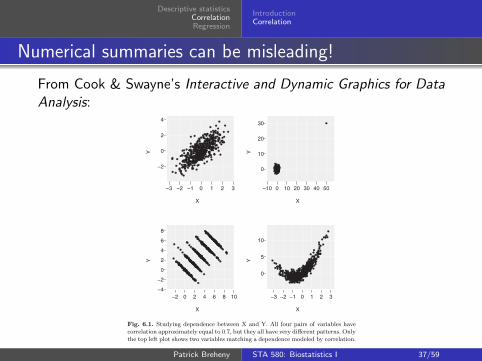
Numerical summaries can be misleading!
From Cook & Swayne’s Interactive and Dynamic Graphics for DataAnalysis:
130 6 Miscellaneous Topics
is negative rather than positive. The plot at bottom right shows two variableswith some positive linear dependence, but the obvious non-linear dependenceis more interesting.
−2
0
2
4
−3 −2 −1 0 1 2 3
●
●
●
●
●
●
●
●
●
● ●
●
● ●
●
●
●
●
●●
●
●
●
●
●●
●●
●
●●
●
●
●
●
●
●
●
●
●
●
●
●
●
●●
●
●●
●
●●
●
●
● ●
●
●
●
●●
●
●
●
●
●●
●
●
●
●
●●
● ●
●
●
●
●
●
●
●
●
●
●●
●
●
●●
●●
●●
●
●
●
●
●
●
●
●●
●●
●
●
●
●
● ●
●
●
●
●
●
●
●
●
●●
●
●
●●
●
●
●
●
●
●
●
●
●●
●
●
●
●
●
●
●
●
●
●
●
●
●
●
●
●
●●
●●
●●●
●●
●
●
●
●
●
●
●
●
●
●
●
●
●
●●
●
●
●
●
●
●●
●
●
●
●
●
●
●
●●
●
●
●
●●
●
●
●●
●
●
●●
●
●
●●
●
●
●
●
●
●
●
●
●
●●
●
●
●
●
●
●
●●
●
●
●
●
●
●
●●
●
●
●
●
●●
●
●
●
●
●
●●
●
●
●
● ●
●
●
●
●
●
●●
●
●
●
●
●
●
●
●
●
●
●
●
●
●
●●
●
● ● ●
●
●
● ●●
●
●
●
●●
●
●
●
●
●●
●
●
●
●
●
●
● ●
●●
●
●
●
●●
●
●●
●
●
●
●
●
●
●
●
●
●
●
●
●
●
●
●
●
●
●
●
●
●
●
●
●
● ●●
●●●
●
●
●
●
●
●●
●● ●
●
● ●
●
●
●
●
●
●
●
●
●
●
●
●
●
●●
●
●●
●
●
●●
●
●
●
●●
●
●
●
●
●
●
●
●
●
●
●
●
●●
●
●
●
●
●
●
●
●
●
●●
●
●
●
●
●
●
●
●
●
●●●●
●
● ●
●
●●
●●
●●
●
●
●
●
● ●
●●●
●
●
● ●
●
●
●●
●
●
●
●
●
●
●
●
●
●
●
●
●
●
●
●●
●●
● ●
● ●
●
●●●
●
●
●
●
●
●
●
●
●
●
●
●
●
●
●●
●
●
●
●
●
●
●
Y
X
0
10
20
30
−10 0 10 20 30 40 50
●
●●
●●●●●●●●●
●
●
●
●
●●●●
●
●●
●●●●●
●
●●●
●
●●
●●●●●●●●
●●
●
●●●●●●●●●●
●
●
●●●●●●●
●●●●●
●●●●●●●
●●●● ●
●●●●●●
●●●
●●
● ●●●●●●●●●●●●●●●●●●
●●●●●
●
●
●●●●●●
●●
●●
●●●●
●●●●●●●●
●●
●● ●
●●●●●●
●
●●
●●
●●
●●
●●●●●●
●●●●●●●●●●●●●●●●
●
●●●●●●●
●●●
●●●●
●
●● ●●●●●●●●●●
●
●●●●
●●●● ●
●●●●
●●
●●●●●●●
● ●●
●● ●●●
●●●
●●●●
●●
●
●●●●
●●●●●
●●●●●●●●●●●●●●
●●●●●
●●●●●●
●
●●●●●●●
●●●
●●●●●●●●●●
●●●●●
●●
●
●●●●
●●
●
●●●●
●●●●●
●●●●
●●
●●●●●●●
●●●●●
●●●●●●●●●●● ●●●●
●
●
●●
●●●
●●
●●●
●●●
●●●●
●●
●●●●●●●●
●●
●
●●●●●●
●● ●●●●●
●●
●●●●●●
●
●
●
●●●●●●●
●●
●●●●●●
●●●●●●●●●●
●●
●●●●●●●●
●●●●●
●●●● ●●●●●●●●
●●●●
●●●
●
●
●●●●●
●
●●●●●●●
●●●●●●
Y
X
−4
−2
0
2
4
6
8
−2 0 2 4 6 8 10
●
●●
●
●
●●
●
●
●
●●
●
●
●●●
●
●
●
●●
●
●●●
●●
●●
●●
●
●
●●
●
●●
●
●
●●
●
●●
●
●●
●
●●
●
●●●
●●
●
●●
●
●●
●●
●
●
●
●●
●●
●
●
●
●
●
●
●
●●
●
●●
●●
●
●
●
●●●●
●
●●
●●
●
●●
●
●●
●
●●
●●
●●
●●
●
●
●
●
●
●
●
●
●●●●
●
●
●●
●●
●
●●
●
●
●
●
●
●
●
●
●
●
●●●
●
●●
●
●●
●
●
●
●
●
●
●
●●●
●●●
●
●
●
●
●●
●
●●●
●●
●
●
●●
●
●●
●●
●
●
●●
●
●
●
●
●
●●
● ●
●●●
●●●
●●
●●
●●
●
●
●
●
●
●
●
●●
●
●
●●●
●
●
●●
●●
●●
●●●●●●
●●●●●
●
●
●
●
●●
●
●
●
●●
●
●
●
●
●
●●
●
●●
●
●
●●
●
●
●●
●
●●
●●●
●
●
●
●●
●●
●●
●
●●
●
●
●
●
●
●●
●
●●
●●
●
●
●
●
●●
●●
●
●
●●
●●
●
●
●●
●●
●●●
●
●
●
●●●
●
●
●●●
●
●
●
●
●●
●●●●●
●
●●
●
●●●
●
●●●●
●
●
●
●
●●
●●●
●
●●
●●●
●●●●
●●
●
●
●
●●
●
●
●●
●●
●●●
●●
●
●
●
●
●
●
●
●●
●●
●
●●
●●
●●●
●●
●
●
●●●
●●
●●●
●●●
●
●
●
●
●
●
●
●●
●●
●
●
●
●●●
●
●●
●
●
●
●
●●
●
●
●
●
●
●●
●
●●
●●●
●
●●
●●
●
●
●
●
●
●
●
●●
●
●
●
●●
●
●
●●
●●●●
●
Y
X
0
5
10
−3 −2 −1 0 1 2 3
●
●
●
●
●
●
●
●
●
●
●
●
●
●
●
●
●
●
●
●
●
●
●
●
●●
●●
●
●
●
●●
●
●
●
●
●
●
●
●
●
●●●
●●●
●●
● ●●●
●
●●
●
●
●
●
●
●
●
●
●
●
●
●
●
●
●
●
●
●
●●
●
●
●●●
●
●●●
●
●●
●
●
●
●
●
●
●
●
●●
●
●
●
●●
●
●●
●
●●
●
●
●
●
●
●●●
●●
●
●
●
●●
●
●
●● ●
●
●
●
● ●●
●
●
●
●
●
●●
●
●
●
●●
●
●●
●
●●
●
●●
●
●
●
●
●●
●
●●
●
●
●
●
●
●●
●
●
●
●
●
●
●
●
●
●●●
●
●
●
●
●●●
●
●
●
●
●● ●
●●
●●
●
●
●●
●
●
●
● ●
●
●
●
●
●●
●
●
●
●
●
●
●
●
●
●
●
●
●
● ●●
●●
●●
●
●
●
●
●
●
●
●
●●
●
●●
●
● ●●●
●
●
●
●
●
●
●
●
●
●●
●
●
●
●●
● ●●●
●● ●
●
●
●●●
●
●
●
●● ●
●
●
●
●
●
●
●
●
●
●
●●
●●
●●
●
●
●
●
●●
●
●●
●
●
●
●
●
●●
●
●
●
●
●
●
●
●
●●
●
●
●
●
●
●
●
●●
●
●●●
●●●
● ●
●
●
●●
●
●
●
●
● ●
●
●
●
●
●
●
●
●
●
●●●
●
●
●
●
●
●
●●
●
●
●
●
●
●
●
●
●●
●
●
●
● ●
●
●
●
●
●
●
● ●
●●
●●●
●●
●●
●
●
●
●
●●●
● ●
●
●
●●
●
●
●●
●
●
●
●
● ●●
●
●
●
●
●
●
●
●●
●
●
●
● ●
●
● ●
●●
●
●
●
●
●
●
●
●
●
●
●
●●
●
●
●
●
●
●
●
●
●
●
●
●
●●
●
●
●●
●
●
●
●
●
●
●●
● ●●
●
●
●
Y
X
Fig. 6.1. Studying dependence between X and Y. All four pairs of variables havecorrelation approximately equal to 0.7, but they all have very different patterns. Onlythe top left plot shows two variables matching a dependence modeled by correlation.
With graphics we cannot only detect a linear trend, but virtually any othertrend (nonlinear, decreasing, discontinuous, outliers) as well. That is, we caneasily detect many different types of dependence with visual methods.
The first step in using visual methods to determine whether a pattern is“really there” is to identify an appropriate pair of hypotheses, the null andan alternative. The second step is to determine a process that simulates thenull hypothesis to generate comparison plots. Some common null hypothesisscenarios are as follows:
Patrick Breheny STA 580: Biostatistics I 37/59

Descriptive statisticsCorrelationRegression
IntroductionCorrelation
Ecological correlations
Epidemiologists often look at the correlation between twovariables at the ecological level – say, the correlation betweencigarette consumption and lung cancer deaths per capita
However, people smoke and get cancer, not countries
These correlations have the potential to be misleading
The reason is that by replacing individual measurements bythe averages, you eliminate a lot of the variability that ispresent at the individual level and obtain a higher correlationthan there really is
Patrick Breheny STA 580: Biostatistics I 38/59

Descriptive statisticsCorrelationRegression
IntroductionCorrelation
Fat in the diet and cancer
From an article by Carroll in Cancer Research (1975):
Patrick Breheny STA 580: Biostatistics I 39/59
Descriptive statisticsCorrelationRegression
Regression and correlationThe regression fallacy
NHANES
Every few years, the CDC conducts a huge survey of randomlychosen Americans called the National Health and NutritionExamination Survey (NHANES)
Hundreds of variables are measured on these individuals:
Demographic variables like age, education, and incomePhysiological variables like height, weight, blood pressure, andcholesterol levelsDietary habitsDisease statusLots more: everything from cavities to sexual behavior
Patrick Breheny STA 580: Biostatistics I 40/59

Descriptive statisticsCorrelationRegression
Regression and correlationThe regression fallacy
Predicting weight from height
For the 2,649 adult women in the NHANES data set:
average height = 5 feet, 3.5 inchesaverage weight = 166 poundsSD(height) = 2.75 inchesSD(weight) = 44.5 poundscorrelation between height and weight = 0.3
Suppose you were asked to predict a person’s weight fromtheir height
First, an easy case: suppose the woman was 5 feet, 3.5 inches
Since the woman is average height, we have no reason toguess anything other than the average weight, 166 pounds
Patrick Breheny STA 580: Biostatistics I 41/59

Descriptive statisticsCorrelationRegression
Regression and correlationThe regression fallacy
Predicting weight from height (cont’d)
How about a woman who is 5’6?
She’s a bit taller than average, so she probably weighs a bitmore than average
But how much more?
To put the question a different way, she is almost onestandard deviation above the average height; how manystandard deviations above the average weight should weexpect her to be?
Patrick Breheny STA 580: Biostatistics I 42/59
Descriptive statisticsCorrelationRegression
Regression and correlationThe regression fallacy
Using the correlation coefficient
The answer turns out to depend on the correlation coefficient
Since the correlation coefficient for this data is 0.3, we wouldexpect the woman to be 0.3 standard deviations above themean weight, or 166 + 0.3(44.5) = 179 pounds
Patrick Breheny STA 580: Biostatistics I 43/59

Descriptive statisticsCorrelationRegression
Regression and correlationThe regression fallacy
Graphical interpretation
●●
●
●
●
●
●
●
●
●
●●
●
●
●
●
●
●
●
●
●
●
●
●
●
●
●
●
●
●
● ●
●
● ●
●
●
●
●
●
●
●
●
●
●
●
●
●
●
●
●●
● ●
●
●
●
●
●
●
●
●
●
●
●
●
●
●
●
●
●
●
● ●
●●
●
●
●
● ●
●
●
●●
●
●
●
●
●
●
●
●
●
●
●
●
●
●
●
●
●
●
●
●
●
●
●
●
●●
●
●
●
●
●
●●
●
●
●
●
●
●
●
●
●
●
●
●
●
●●
●●
●
●
●
●
●
●
●
●
●
● ●
●
●
●
●
●●
●
●
●
●
●
●
●
●
●
●
●
●●●
●
●
●
●
●●
●
●
●
●
●
●
●
●
●
●
●
●
●
●
●
●
●
●
●
●
● ●
●
●
●
●
●
●
●
●
●
●
●
●
●
●
●
●
●
●
●
●
●
●
●
●
●●
●
●
●
●
●
●
●
●
●
●●
●
●
●
●
●
●●
●
●
● ●
●
●
●
●
●
●
●
●
●
●
●
●
●
●
●
●
●
●
●
●
●
●
●
●●
●
●
●
● ●
●
●
●●
●
●
●
●
●
●
●
●
●
●
●
●
●
●
●●
●
●
●
●
●
●
●
●
●
●
●
●
●
●
●
●
●
●
●
●
●
●
●
●
●
●
●
●
●
●●
●
●
●
●
●
●●
●
●
●
●
●
●
●● ●
●
●
●
●●
●
●●
●
●
●●
●
●
●
●
●
●
●
●
●
●
●
●
●
●
●
●
●
●●
●
●● ●
●
●
●
●
●
●
●
●●
●
●
●●
●●
●
●
●
●
●
●
●
●
●
●
●
●
●
●
●
●
●
●
●
●
●
●
●● ●
●
●
●●
●
●
●
●
●
●
●
●
●
●
●
●
●
● ●
●
●
●
●
●●
●
●
●
●●
●
●
●
●
●●
●
●
●
●
●
●
●
●
●●
●
●
●
●
●
●
●
●
●
●
●
●
●
●
●
●
●
●
●
●
●
●
● ●
●●
●
●
●
●
●● ●
●
●
●
●●
●
●
●
●
●
●
●
●
●
●●
●
●
●
● ●
●
●
●●
●
●
●●
●
●
●
●
●
●
●
●
●
●
●
●
●
●
●
●
●
●
●
●
●
●
●
●
●
●
●
●
●
●
● ●
●
●●
●
●
●
●
●
●
●●
●
●●
● ●
●
●
●●
●
●
●
●
● ●●
●
●
●
●
●●●
●
●
●
●
●
●
●
●
●
●
●
●
●●
●
●●
●
●
●
●
●
●
●
●
●
●●
●
●
● ●
●
●
●
●
●
●
●
●
●
●
●
●
●
●
●
●
●
●
●●
●
●
●
●
●
●
●●
●
●
●●
●●
●
●
●
●
●
●
●
●
●
●
●
●
●
●
●
●
●
●
●
●
●
●
●
●
●
●
●
●
●
●
●
●
●
●
●
●
●
●
●
●
●
●
●
●
●
●
●● ●
●●
●
●
●
●
●●
●
●
●
●
●
●
●
●
●
●
●
●
●
●
●
●
●
●
●
●
●
●
●
●
●
●
●
●
●
●
●
●
●
●
●
●
●
● ●
●
●
●
●
●
●
●
●
●
●
●
●
●
●
●●
●
●●
●
●
●
●
●
●
●
●
●
●
●
●
●
●
●
●
●●
●
●
●
●
●
●
●
●
●
●
●
●
●
●
●
●
●
●●
●
●
●
●
●
●●
●
●●
●
●
●
●
●
●
●
●
●
●
● ●
●
●
●
●
●
●
●
●
●
●
●
●
●
●●
●
●
● ●
●
●
●
●
●
●
●●
●●
●
●
●
●
● ●
●
●
●
●
●
●
●
●
●
●
●
●
●
●
●
●
●
●
●
●
●
●
●
●
●
●
●●
●
●●
●
●
●
●
●
●●
●●
●
●
●●
●
●
●
●
●
●
●
●
●
●●
●●
●●
●
●
●
●
●
●
●
●
●
●
●
●
●
●
●
●
●
●
●
●
●●
●
●
●
●
●
● ●
●
●
●●
●
●
●
●
●
●
●
●
●
●
●
●
●
●
●
●
●●
●
●
●
●
●
●
●
●
●●
●
●
●
●
●
●
●
●
●
●
●
●●●
●
●
●
●
●
●
●
●
●
●
● ●●
●
●
●
●
●
●
●
●
●
●
●
●
●
●
●
●
●
●
●
●
●
●
●
●
●
●
●●
●
●
●
●
●
●
●
●
●
●
●
●
●
● ●
●
●
●
●
●
●
●
●
●
●
●
●
●
●
●
●
●
●
●
●
●
●
●
●●
●
●
●
●●
●
●
●
●
●
●
●
●
●
●
●
●
●
●
●
●
●
●
●
●
●
●●
●
●
●
●
●
●
●
●
●
●
●
●
●
● ●
●
●
●
●
●
●
●●
●
●
●
●
●
●
●
●
●
●
●
●
●
●
●
●
●
●●
●
●
●
●
●
●
●
●
●
●
●
●
●●
●
●
●
●
● ●
●
●
●
●
●
●
●
●
●
●
●
●
●
●●
●
●
●
●
●
●
●
●
●
●
●
●
●
●
●
●●
●
●
●
●
●
●
●
●
●
●
●
●
●
●
●
●
● ●
●
●
●
● ●
●
● ●
●
●
●
●
●
●
●
●
●
●
●
●
●
●
●
●
●
●
●
●
●
●
●
●
●
●
●
●
●
●
●
●
●
●
●
●
●
●●
●
●
●
●
●
●
●
●
●
●
●
●
●
●
●
●
●
●
●
●
●
●
●
●
●
●●
●
● ●
●
●
●
●
●
●
● ●
●
●
●
●
●
●
●
●
●
●
●
●
●
●
●
●
●
●
●
●
●
●
●
●
●
●
●
●
●
●
●
●
●
●
●
●
●
●
●
●
●
●
●
●
●●
●
●
●
●
●
●
●
●●
●
●
●
●
●
●
●
●
●
●●
●
●
●
●●
●
●
●
●●
●
●
●
●
●
●
●
●
●
●
●
●
●●
●
●
●
●
●●
●
●
●
●
●
●
●
●
●
● ●
●
●
●
●
●
●●
●
●
●
●
●
●
●
●
●
●
●
●
●
●
●
●
●
●
●
●
●
●
●
●
●
●
●
●
●
●
●
●
●
●
●
●
●
●
●
●
●
●
●
●
●
●
●
●
●
●●●
●
●●
●
●
●
●
●
●
●
●
●●
●
●
●
●
● ●
●
●
●
●
●
●
●
●
●
●
●
●
●
●
●
●
●
●
●
●
●
●●
●
●
●
●
●
●
●
●
●
●
●
●
●
●
●
●
●
●●
●
●
●●
●
●●
●
●
●●
●
●
●
●
●
●
●
●
●
●
●
●
●
●
●
●
●
●
●
●
●
●
●
●
●
●
●
●
●
●
●
●
●
●
●
●
●
●
●
●
●
●
●
● ●
●
●
●
●
●
●
●
●
●
●
●
●
●
●
●
●
●
●
●
●
●
●
●
●
●
●
●
●
●
●
●
●
●
●
●●
●
●
●
●●
●
●
●
●
●
●●
●
●
●
●
●
●
●
●
●
●
●
●
●
●
●
●
●
●
●
●
●
●
●
●●
●
●
●
●
●
●
●●
●
●
●
●
●
●
●●
●
●
●
●
●
●
●
●
●
●
●
●
●
●
●
●
●
●
●
●
●
●
●
●
●
●
●
●
●
●
●
●
●
●
●
●
●
●
●
●
●●
●
●● ●
●
●
●
●
●
●
●
●●
●
●
●
●
●
●
●
●
●
●
●
●
●
●
●
●
●
●
●
●
●
●
●
●
●
●
●
●●
●
●
●
● ●
●
●
● ●
●
●
●
●
●
●
●
●
●
●
●
●
●
●
●
●
●
●
●
●
●
●
●
●
●
●
●
●
●
●
●
●
●●
●
●●
●
●
●●
●
●
●
●
●
●
●
●
●
●
●
●
●
●
●
●
●
●
●
●
●
●
●
●
●
●
●
●
●
●
●
●●
●
●
●
●
●
●
●
●
●
●
●
●●
●
●
● ●
●
●
●
●
●
●
●
●
●
●●
●
●
●
●
●
●
●
●
●
●
●
●
●
●
●
●
●
●
●
●
●
●
●
●
●
●
●
●
●●
●
●
●
●
●●
●
●
●
●
●
●●
●
●
●
●
●
●
●
●
●
●●
●
●
●
●
●
●
●
●
●
●
●●
●● ●●
●
●
●
●
●
●
●
●
●
●
●
●
●
●
●
●
●
●
●
●
●
●
●
●
●
●
●
●●
●
●
●
●
●
●
●
●
●
●
●
●
●
●
●
●
●
●
●
●
●●
●
●
●
●
●
●
●
●
●
●
●
●
●
●
●
●
●
●●
●
●
●●
●
●
●
●
●
●
●
●
●
●
●
●
●
●
●
●
●
●
●
●
●●
●
●●
●
●
●
●
●
●
●
●
●
●
●
●
●
●●
●
●
●
●●
●
●
●
●
●
●
●
●
●
●
● ●
●●
●
●
●
● ●
●
●
●
●
●
●
●
●
●
●●
●●
●
●
●
●
●
●
●
●
●
●
●●
●
●
● ●
●
●
●
●
●●
●
●
●
●
●
●●
●
●
●
●
●
●
●
●
●
●
●
●●
●
●
●
●
●
●
●
●
●
●
●
●
●
●
●
●
●
●
●
●
●
●
●
●
●
●
●
●
●
●
●
●
●
●
●
●
●
●
●
●
●
●
●
●
●
●
●
●
●
●
●
●
●
●
●●
●
●
●
●
●
●
●●
●
●●
●
●
●
●
●
●●
●
●
●
●
●
●
●
●
●
●
●
●
●
●
●●
●
●
●
●
●
●
●●
●●
●
●
●
●
●
●
●
●
●
●
●
●
●
●
●
●
●
●●
●
●●
●
●
●
●
●
●
●●
●
●
●
●
●
●
●
●
●
●
●
●
●
●●
● ●
●
●
●●
●
●
●
●
●
●
●
●
●●
●
●
●
●
●
●
●
●
●
●
●
●
●
●●
●
● ●
●
●
●
●
●
●
●
●
●
●
●
●
●
●
●
●
●
●
●
●
●
●
●
●
●
●
●
●
●
●
●
●
●
●
●
●
●
●
●
●●
●
●
●
●
●
●
●
●
●
●
●
●
●
●
●
●
●
●
●
●
●
●
●
●
●
●
● ●
●
●
●●
●
●
●
●
●
●●
●
●
●
●
●
●
●
●
●
● ●
●
●
●
●
●
●
●●
●
●
●
●
●
●
●
●
●
●
●
●●
●
●
●
●
●
●
●
●
●
●
●
●
● ●
●
●
●
●
●
●
●
●
●
●
●
●
●
●
●
●
●
●
●
●
●
●
●
●
●
●
●●
●
●
●
●●
●
●
●
●
●
●
●●
●
●
●
●
●
●
●
●
●
●
●
●
●
●
●●
●
● ●
●
●
●
●
●
●
●
●
●
●
●
●
●
●
●
●●
●
●
●
●
●
●
●
●
●
●
●
●
●
●
●
●
●
●
●
●●
●
●
●
●
●
●
●
●
●
●
●
●
●
●
●
●
●
●
●
●
●
●
●
●
●
●
●
●
●
●●
●
●
●
●
●
●
●
●
●
●
●
●
●
●
●
●
●
●
●
●
●
●
●
●
●
●
●
●
●●
●
●●
●
●
●
●
●
●●
● ●
●
●
●
●
●●
●
●
●
●
●
●
●
●●
●
●
●
●
●
●
●
●
● ●
●●
●
●
●
●
●
●
●
●
●
●
●
●
●
55 60 65 70
100
200
300
400
Height (inches)
Wei
ght (
lbs)
Patrick Breheny STA 580: Biostatistics I 44/59

Descriptive statisticsCorrelationRegression
Regression and correlationThe regression fallacy
The regression line
This line is called the regression line
It tells you, for any height, the average weight for women ofthat height
Here, we were trying to predict one variable based on oneother variable; if we were trying to predict weight based onheight, dietary habits, and cholesterol levels, or trying to studythe relationship between cholesterol and weight whilecontrolling for height, then this is called multiple regression
Multiple regression is beyond the scope of this course, but is amajor topic in Biostatistics II
Patrick Breheny STA 580: Biostatistics I 45/59

Descriptive statisticsCorrelationRegression
Regression and correlationThe regression fallacy
The equation of the regression line
Like all lines, the regression line may be represented by theequation
y = α+ βx,
where α is the intercept and β is the slope
For the height/weight NHANES data, the intercept is -137pounds and the slope is 4.8 pounds/inch
Patrick Breheny STA 580: Biostatistics I 46/59

Descriptive statisticsCorrelationRegression
Regression and correlationThe regression fallacy
β vs. r
Note the similarity and the difference between the slope of theregression line (β) and the correlation coefficient (r):
The correlation coefficient says that if you go up in height byone standard deviation, you can expect to go up in weight byr = 0.3 standard deviationsThe slope of the regression line tells you that if you go up inheight by one inch, you can expect to go up in weight byβ = 4.8 pounds
Essentially, they tell you the same thing, one in terms ofstandard units, the other in terms of actual units
Therefore, if you know one, you can always figure out theother simply by changing units (which here involvesmultiplying by the ratio of the standard deviations)
Patrick Breheny STA 580: Biostatistics I 47/59
Descriptive statisticsCorrelationRegression
Regression and correlationThe regression fallacy
β vs. r (cont’d)
Suppose a woman’s height is increased one inch; what do weexpect to happen to her weight?
1 inch = 1/2.75 SDs
An increase of 1/2.75 SDs in height means an increase in0.3/2.75 SDs in weight
0.3/2.75 SDs = 0.3(44.5/2.75) = 4.8 pounds
Patrick Breheny STA 580: Biostatistics I 48/59
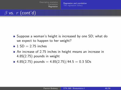
Descriptive statisticsCorrelationRegression
Regression and correlationThe regression fallacy
β vs. r (cont’d)
Suppose a woman’s height is increased by one SD; what dowe expect to happen to her weight?
1 SD = 2.75 inches
An increase of 2.75 inches in height means an increase in4.85(2.75) pounds in weight
4.85(2.75) pounds = 4.85(2.75)/44.5 = 0.3 SDs
Patrick Breheny STA 580: Biostatistics I 49/59

Descriptive statisticsCorrelationRegression
Regression and correlationThe regression fallacy
There are two regression lines
We said that the correlation between weight and height is thesame as the correlation between height and weight
This is not true for regression
The regression of weight on height will give a different answerthan the regression of height on weight
Patrick Breheny STA 580: Biostatistics I 50/59

Descriptive statisticsCorrelationRegression
Regression and correlationThe regression fallacy
The two regression lines
●●
●
●
●
●
●
●
●
●
●●
●
●
●
●
●
●
●
●
●
●
●
●
●
●
●
●
●
●
● ●
●
● ●
●
●
●
●
●
●
●
●
●
●
●
●
●
●
●
●●
● ●
●
●
●
●
●
●
●
●
●
●
●
●
●
●
●
●
●
●
● ●
●●
●
●
●
● ●
●
●
●●
●
●
●
●
●
●
●
●
●
●
●
●
●
●
●
●
●
●
●
●
●
●
●
●
●●
●
●
●
●
●
●●
●
●
●
●
●
●
●
●
●
●
●
●
●
●●
●●
●
●
●
●
●
●
●
●
●
● ●
●
●
●
●
●●
●
●
●
●
●
●
●
●
●
●
●
●●●
●
●
●
●
●●
●
●
●
●
●
●
●
●
●
●
●
●
●
●
●
●
●
●
●
●
● ●
●
●
●
●
●
●
●
●
●
●
●
●
●
●
●
●
●
●
●
●
●
●
●
●
●●
●
●
●
●
●
●
●
●
●
●●
●
●
●
●
●
●●
●
●
● ●
●
●
●
●
●
●
●
●
●
●
●
●
●
●
●
●
●
●
●
●
●
●
●
●●
●
●
●
● ●
●
●
●●
●
●
●
●
●
●
●
●
●
●
●
●
●
●
●●
●
●
●
●
●
●
●
●
●
●
●
●
●
●
●
●
●
●
●
●
●
●
●
●
●
●
●
●
●
●●
●
●
●
●
●
●●
●
●
●
●
●
●
●● ●
●
●
●
●●
●
●●
●
●
●●
●
●
●
●
●
●
●
●
●
●
●
●
●
●
●
●
●
●●
●
●● ●
●
●
●
●
●
●
●
●●
●
●
●●
●●
●
●
●
●
●
●
●
●
●
●
●
●
●
●
●
●
●
●
●
●
●
●
●● ●
●
●
●●
●
●
●
●
●
●
●
●
●
●
●
●
●
● ●
●
●
●
●
●●
●
●
●
●●
●
●
●
●
●●
●
●
●
●
●
●
●
●
●●
●
●
●
●
●
●
●
●
●
●
●
●
●
●
●
●
●
●
●
●
●
●
● ●
●●
●
●
●
●
●● ●
●
●
●
●●
●
●
●
●
●
●
●
●
●
●●
●
●
●
● ●
●
●
●●
●
●
●●
●
●
●
●
●
●
●
●
●
●
●
●
●
●
●
●
●
●
●
●
●
●
●
●
●
●
●
●
●
●
● ●
●
●●
●
●
●
●
●
●
●●
●
●●
● ●
●
●
●●
●
●
●
●
● ●●
●
●
●
●
●●●
●
●
●
●
●
●
●
●
●
●
●
●
●●
●
●●
●
●
●
●
●
●
●
●
●
●●
●
●
● ●
●
●
●
●
●
●
●
●
●
●
●
●
●
●
●
●
●
●
●●
●
●
●
●
●
●
●●
●
●
●●
●●
●
●
●
●
●
●
●
●
●
●
●
●
●
●
●
●
●
●
●
●
●
●
●
●
●
●
●
●
●
●
●
●
●
●
●
●
●
●
●
●
●
●
●
●
●
●
●● ●
●●
●
●
●
●
●●
●
●
●
●
●
●
●
●
●
●
●
●
●
●
●
●
●
●
●
●
●
●
●
●
●
●
●
●
●
●
●
●
●
●
●
●
●
● ●
●
●
●
●
●
●
●
●
●
●
●
●
●
●
●●
●
●●
●
●
●
●
●
●
●
●
●
●
●
●
●
●
●
●
●●
●
●
●
●
●
●
●
●
●
●
●
●
●
●
●
●
●
●●
●
●
●
●
●
●●
●
●●
●
●
●
●
●
●
●
●
●
●
● ●
●
●
●
●
●
●
●
●
●
●
●
●
●
●●
●
●
● ●
●
●
●
●
●
●
●●
●●
●
●
●
●
● ●
●
●
●
●
●
●
●
●
●
●
●
●
●
●
●
●
●
●
●
●
●
●
●
●
●
●
●●
●
●●
●
●
●
●
●
●●
●●
●
●
●●
●
●
●
●
●
●
●
●
●
●●
●●
●●
●
●
●
●
●
●
●
●
●
●
●
●
●
●
●
●
●
●
●
●
●●
●
●
●
●
●
● ●
●
●
●●
●
●
●
●
●
●
●
●
●
●
●
●
●
●
●
●
●●
●
●
●
●
●
●
●
●
●●
●
●
●
●
●
●
●
●
●
●
●
●●●
●
●
●
●
●
●
●
●
●
●
● ●●
●
●
●
●
●
●
●
●
●
●
●
●
●
●
●
●
●
●
●
●
●
●
●
●
●
●
●●
●
●
●
●
●
●
●
●
●
●
●
●
●
● ●
●
●
●
●
●
●
●
●
●
●
●
●
●
●
●
●
●
●
●
●
●
●
●
●●
●
●
●
●●
●
●
●
●
●
●
●
●
●
●
●
●
●
●
●
●
●
●
●
●
●
●●
●
●
●
●
●
●
●
●
●
●
●
●
●
● ●
●
●
●
●
●
●
●●
●
●
●
●
●
●
●
●
●
●
●
●
●
●
●
●
●
●●
●
●
●
●
●
●
●
●
●
●
●
●
●●
●
●
●
●
● ●
●
●
●
●
●
●
●
●
●
●
●
●
●
●●
●
●
●
●
●
●
●
●
●
●
●
●
●
●
●
●●
●
●
●
●
●
●
●
●
●
●
●
●
●
●
●
●
● ●
●
●
●
● ●
●
● ●
●
●
●
●
●
●
●
●
●
●
●
●
●
●
●
●
●
●
●
●
●
●
●
●
●
●
●
●
●
●
●
●
●
●
●
●
●
●●
●
●
●
●
●
●
●
●
●
●
●
●
●
●
●
●
●
●
●
●
●
●
●
●
●
●●
●
● ●
●
●
●
●
●
●
● ●
●
●
●
●
●
●
●
●
●
●
●
●
●
●
●
●
●
●
●
●
●
●
●
●
●
●
●
●
●
●
●
●
●
●
●
●
●
●
●
●
●
●
●
●
●●
●
●
●
●
●
●
●
●●
●
●
●
●
●
●
●
●
●
●●
●
●
●
●●
●
●
●
●●
●
●
●
●
●
●
●
●
●
●
●
●
●●
●
●
●
●
●●
●
●
●
●
●
●
●
●
●
● ●
●
●
●
●
●
●●
●
●
●
●
●
●
●
●
●
●
●
●
●
●
●
●
●
●
●
●
●
●
●
●
●
●
●
●
●
●
●
●
●
●
●
●
●
●
●
●
●
●
●
●
●
●
●
●
●
●●●
●
●●
●
●
●
●
●
●
●
●
●●
●
●
●
●
● ●
●
●
●
●
●
●
●
●
●
●
●
●
●
●
●
●
●
●
●
●
●
●●
●
●
●
●
●
●
●
●
●
●
●
●
●
●
●
●
●
●●
●
●
●●
●
●●
●
●
●●
●
●
●
●
●
●
●
●
●
●
●
●
●
●
●
●
●
●
●
●
●
●
●
●
●
●
●
●
●
●
●
●
●
●
●
●
●
●
●
●
●
●
●
● ●
●
●
●
●
●
●
●
●
●
●
●
●
●
●
●
●
●
●
●
●
●
●
●
●
●
●
●
●
●
●
●
●
●
●
●●
●
●
●
●●
●
●
●
●
●
●●
●
●
●
●
●
●
●
●
●
●
●
●
●
●
●
●
●
●
●
●
●
●
●
●●
●
●
●
●
●
●
●●
●
●
●
●
●
●
●●
●
●
●
●
●
●
●
●
●
●
●
●
●
●
●
●
●
●
●
●
●
●
●
●
●
●
●
●
●
●
●
●
●
●
●
●
●
●
●
●
●●
●
●● ●
●
●
●
●
●
●
●
●●
●
●
●
●
●
●
●
●
●
●
●
●
●
●
●
●
●
●
●
●
●
●
●
●
●
●
●
●●
●
●
●
● ●
●
●
● ●
●
●
●
●
●
●
●
●
●
●
●
●
●
●
●
●
●
●
●
●
●
●
●
●
●
●
●
●
●
●
●
●
●●
●
●●
●
●
●●
●
●
●
●
●
●
●
●
●
●
●
●
●
●
●
●
●
●
●
●
●
●
●
●
●
●
●
●
●
●
●
●●
●
●
●
●
●
●
●
●
●
●
●
●●
●
●
● ●
●
●
●
●
●
●
●
●
●
●●
●
●
●
●
●
●
●
●
●
●
●
●
●
●
●
●
●
●
●
●
●
●
●
●
●
●
●
●
●●
●
●
●
●
●●
●
●
●
●
●
●●
●
●
●
●
●
●
●
●
●
●●
●
●
●
●
●
●
●
●
●
●
●●
●● ●●
●
●
●
●
●
●
●
●
●
●
●
●
●
●
●
●
●
●
●
●
●
●
●
●
●
●
●
●●
●
●
●
●
●
●
●
●
●
●
●
●
●
●
●
●
●
●
●
●
●●
●
●
●
●
●
●
●
●
●
●
●
●
●
●
●
●
●
●●
●
●
●●
●
●
●
●
●
●
●
●
●
●
●
●
●
●
●
●
●
●
●
●
●●
●
●●
●
●
●
●
●
●
●
●
●
●
●
●
●
●●
●
●
●
●●
●
●
●
●
●
●
●
●
●
●
● ●
●●
●
●
●
● ●
●
●
●
●
●
●
●
●
●
●●
●●
●
●
●
●
●
●
●
●
●
●
●●
●
●
● ●
●
●
●
●
●●
●
●
●
●
●
●●
●
●
●
●
●
●
●
●
●
●
●
●●
●
●
●
●
●
●
●
●
●
●
●
●
●
●
●
●
●
●
●
●
●
●
●
●
●
●
●
●
●
●
●
●
●
●
●
●
●
●
●
●
●
●
●
●
●
●
●
●
●
●
●
●
●
●
●●
●
●
●
●
●
●
●●
●
●●
●
●
●
●
●
●●
●
●
●
●
●
●
●
●
●
●
●
●
●
●
●●
●
●
●
●
●
●
●●
●●
●
●
●
●
●
●
●
●
●
●
●
●
●
●
●
●
●
●●
●
●●
●
●
●
●
●
●
●●
●
●
●
●
●
●
●
●
●
●
●
●
●
●●
● ●
●
●
●●
●
●
●
●
●
●
●
●
●●
●
●
●
●
●
●
●
●
●
●
●
●
●
●●
●
● ●
●
●
●
●
●
●
●
●
●
●
●
●
●
●
●
●
●
●
●
●
●
●
●
●
●
●
●
●
●
●
●
●
●
●
●
●
●
●
●
●●
●
●
●
●
●
●
●
●
●
●
●
●
●
●
●
●
●
●
●
●
●
●
●
●
●
●
● ●
●
●
●●
●
●
●
●
●
●●
●
●
●
●
●
●
●
●
●
● ●
●
●
●
●
●
●
●●
●
●
●
●
●
●
●
●
●
●
●
●●
●
●
●
●
●
●
●
●
●
●
●
●
● ●
●
●
●
●
●
●
●
●
●
●
●
●
●
●
●
●
●
●
●
●
●
●
●
●
●
●
●●
●
●
●
●●
●
●
●
●
●
●
●●
●
●
●
●
●
●
●
●
●
●
●
●
●
●
●●
●
● ●
●
●
●
●
●
●
●
●
●
●
●
●
●
●
●
●●
●
●
●
●
●
●
●
●
●
●
●
●
●
●
●
●
●
●
●
●●
●
●
●
●
●
●
●
●
●
●
●
●
●
●
●
●
●
●
●
●
●
●
●
●
●
●
●
●
●
●●
●
●
●
●
●
●
●
●
●
●
●
●
●
●
●
●
●
●
●
●
●
●
●
●
●
●
●
●
●●
●
●●
●
●
●
●
●
●●
● ●
●
●
●
●
●●
●
●
●
●
●
●
●
●●
●
●
●
●
●
●
●
●
● ●
●●
●
●
●
●
●
●
●
●
●
●
●
●
●
55 60 65 70
100
200
300
400
Height (inches)
Wei
ght (
lbs)
Patrick Breheny STA 580: Biostatistics I 51/59
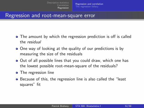
Descriptive statisticsCorrelationRegression
Regression and correlationThe regression fallacy
Regression and root-mean-square error
The amount by which the regression prediction is off is calledthe residual
One way of looking at the quality of our predictions is bymeasuring the size of the residuals
Out of all possible lines that you could draw, which one hasthe lowest possible root-mean-square of the residuals?
The regression line
Because of this, the regression line is also called the “leastsquares” fit
Patrick Breheny STA 580: Biostatistics I 52/59

Descriptive statisticsCorrelationRegression
Regression and correlationThe regression fallacy
Why only r standard deviations?
Only moving r standard deviations away from the averagemay be counterintuitive; if height goes up by one SD,shouldn’t weight too?Here’s an example that I hope will help clarify this concept:
A student is taking her first course in statistics, and we wantto predict whether she will do well in the course or notSuppose we know that last semester, she got an A in mathNow suppose that we know that last semester, she got an A inpottery
These two pieces of information are not equally informativefor predicting how well she will do in her statistics class
We need to balance our baseline guess (that she will receivean average grade) with this new piece of information, and thecorrelation coefficient tells us how much weight the newinformation should carry
Patrick Breheny STA 580: Biostatistics I 53/59
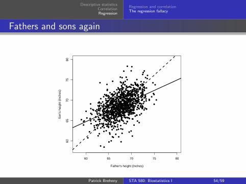
Descriptive statisticsCorrelationRegression
Regression and correlationThe regression fallacy
Fathers and sons again
●
● ●
●
● ●●●
●
●
● ●●
● ●
●●
●
●
●●
●
●●
●●●
●
●● ●●
●
●
●●
● ● ●
●●
●●
●●
●●
●
●
●
●● ●
●● ●
●
●●
●
●● ●
●●
●●●
● ●●
●
●
●
●●● ●●
●
●●
●
●
●●●
●●
●●
●
●
●●
●
●●
●
●●
●
●
● ●
●
● ●●
●
●● ●
●●
●
● ●●●
●●
●●●
●
●
●
●●
●
● ● ●
●●●
●● ●
●
●
●●
●
●●●●
●●●
●● ●
●
● ●
●
●
●●
●●
●
●●
●●
●●
●●●
●
●●
●
●
●
●●
●
●● ●
●●●
●●
●●
●
●●
● ●
● ●●
●●
●
●
●
●
●
●
●
●
●
●
●
●
●
●
● ●
●
● ●
●
●
●●
● ●
●
●●●
● ●
●
●
●
● ●
● ●● ● ●●●
●●
●
●
●●
●
●
● ●
●●
● ●●
●
●
●
●●
● ●●
●
●
●●
●
●
●●
●●
●●
●●● ●
●
●
●●
● ● ●● ● ●
●●
●●
● ●
● ●●
●● ●
●
●●
●●
●●●
●●
●●●
●●
●
●
● ●●
●●
●
●● ● ●
●
●
● ●●●●
●
●
●●
● ●●●
● ● ●●● ●
●
●●●
●● ●
●
●●
● ●●
●
●
●● ●
●
●●
●●
●
● ●●●● ●●
●
●●
● ●
●
●
● ● ●●
●● ●
●
●●●
●●
●●●
● ●
●
●
●
●
●●
●
●
●
●
●
●
●
●
●
●
●
●
●
●
●
●●
●
●
● ●●
●
●
●
●
●
●●●
●●
● ●●
●
● ●●
●●
●●
●
●
●
●
●●● ●●
●
●●
●
●
●●
●
●
●
●
●●
●●●
●●
● ●●
●●●●●● ● ●
●●
●●
●
●
●●
●●●
●●
●● ●
●●●
●● ●
●●●
●
●●●●
●
●●
●
● ●●
●●
●
●
●●●
●●● ●●
●●●
●●●
●●●
●
●●
●
●
●
●
●
●●
●●
●
●●●
●
●
●
●
●●
●
●●
● ●
●●
●
●
●
● ● ● ●●
●●
●●
●
●
● ●●
●
●● ●
●
●
●●
●● ●
●
●●
● ●
●
●
● ●● ●
●
● ●
●
●
●●●
●
●
●
●
●
●
●●
●
●
●
●
●
●
●
●
●
● ●●
●
●
●●
●●
●
●●
●
● ●●
●●
●
●●
●
● ●● ● ●●
●●●
●●
●
● ●
● ● ●
●● ● ●
●
●
●
●
●
●● ● ●●●
● ●
● ●
●
●
●●● ●●
●●
●
●●
●●
●
●●
●● ●●● ●
●●●
●● ●
●
● ●
●
●
●●●
● ●●
●
●●● ●
● ●●
●●
●●
●●
●●
●● ●
●
● ●
● ●
●
●●● ●
●●
●
●
● ●●
●
●●
●
●●
●●●●●
● ●●
●
● ●●●● ●
●●
●
●
● ●●
●●●●
●
●
●
●
● ●●●
●
●
●● ● ●
●●
● ●
●
●●
●
●●
●
● ●
●
●
●
●●
●
●
●
●
●
●
●
●
●
●
●
●
●
●
●
●
●●
●● ● ● ●
●●
●
●
●●●
●●
●
● ●
● ●
●
●
● ●● ●●
● ●●●
●●
●●
●
●
● ●
●● ●
●●
●
●
●
●
●
●●●
●
●
●
●●●
●
●
●
●● ● ●●
● ●●
●●
●
●●
●
●
●●●● ●
●●
●●
●●●
●
●
● ●● ●●
●●●
●●
● ●●
●
●● ●
● ●●●
●
●●
●●
●●●
●●●
●●
●●
●
●●
●● ●
●
●
●●
● ●
●
●●
●
● ● ●● ●
●●●●
●
● ●● ●
●
●●●
●
●●● ●●
●●●
●●
●
●
●
●●
●
●
●●
●●
●●
●●●
● ●
●●
●
●
●●
●
● ● ● ●
●
●
●
●
●
●
●
●
●
●
●
●●
●
60 65 70 75 80
6065
7075
80
Father's height (Inches)
Son
's h
eigh
t (In
ches
)
Patrick Breheny STA 580: Biostatistics I 54/59

Descriptive statisticsCorrelationRegression
Regression and correlationThe regression fallacy
How regression got its name
Because the correlation coefficient is always less than 1, theregression line will always lie beneath the “x goes up by 1 SD,y goes up by 1 SD” rule
Galton called this phenomenon “regression to mediocrity,”and this is where regression gets its name
People frequently read too much into the regression effect –this is called the regression fallacy
Patrick Breheny STA 580: Biostatistics I 55/59

Descriptive statisticsCorrelationRegression
Regression and correlationThe regression fallacy
The regression fallacy, example #1
A group of subjects are recruited into a study
Their initial blood pressure is taken, then they take an herbalsupplement for a month, and their blood pressure is takenagain
The mean blood pressure was the same, both before and after
However, subjects with high blood pressure tended to havelower blood pressure one month later, and subjects with lowblood pressure tended to have higher blood pressure later
Does this supplement act to stabilize blood pressure?
Patrick Breheny STA 580: Biostatistics I 56/59

Descriptive statisticsCorrelationRegression
Regression and correlationThe regression fallacy
Why the does regression to the mean happen?
Not really; the same effect would occur if they took placebo
Why?
Consider a person with a blood pressure 2 SDs above average
It’s possible that the person has a true blood pressure 1 SDabove average, but happened to have a high firstmeasurement; it’s also possible that the person has a trueblood pressure 3 SDs above average, but happened to have alow first measurement
However, the first explanation is much more likely
Patrick Breheny STA 580: Biostatistics I 57/59

Descriptive statisticsCorrelationRegression
Regression and correlationThe regression fallacy
The regression fallacy, example #2
In professional sports, some first-year players have outstandingyears and win “Rookie of the Year” awards
They often fail to live up to expectations in their second years
Writers call this the “sophomore slump”, and come up withelaborate explanations for it
Patrick Breheny STA 580: Biostatistics I 58/59

Descriptive statisticsCorrelationRegression
Regression and correlationThe regression fallacy
The regression fallacy, example #3
An instructor standardizes her midterm and final so that theclass average is 50 and the SD is 10 on both tests
She has taught this class many times and the correlationbetween the tests is always around 0.5
This year, she decides to do something different – she takesthe 10 students with the lowest scores on the midterm andgives them special tutoring
On the final, all ten students score above 50; can this beexplained by the regression effect?
No!
The regression effect can only take these students closer tothe average; the fact that they all score above averageindicates that the tutoring really did work
Patrick Breheny STA 580: Biostatistics I 59/59


