Paul Piveteau - Columbia University

Essays on Global Firms

Paul Piveteau

Submitted in partial fulfillment of the

requirements for the degree

of Doctor of Philosophy

in the Graduate School of Arts and Sciences

Columbia University

2016

c©2016

Paul Piveteau

All Rights Reserved

Abstract

Essays on Global Firms

Paul Piveteau

The field of International Trade aims to study the consequences of the spatial disconnection between

the activities of production and consumption, which has been allowed by the increasing opening of

the economies. However, while most of the history of the field has focused on the role played by

production in shaping trade patterns, only recently researchers have emphasized the importance of

demand characteristics. This dissertation follows these recent works by containing three essays that

specifically study the importance of demand characteristics on export patterns at the microeconomic

level.

In the first chapter of this dissertation, I explore the importance of the dynamic aspects of de-

mand on the export decisions made by firms. Standard dynamic models of trade identify sunk entry

costs as the main export barrier faced by firms. However, these large entry costs are inconsistent

with the existence of many small new exporters with low survival rates in foreign markets. In this

chapter, I study the role of destination-specific demand dynamics by introducing, in a dynamic

model of trade, the idea that firms gradually accumulate consumers in foreign markets. Estimat-

ing the model using export data from individual French firms, I show that this consumer margin

is consistent with the dynamics of sales, prices and survival of exporters, but also leads to much

lower estimates of the entry costs of exporting - about one third of those estimated in the standard

model. Moreover, this change in the nature of trade barriers has important implications at the

aggregate level. In contrast to the standard model, this model correctly replicates the slow response

of trade to shocks and the increasing contribution of the extensive margin in this response. Finally,

I demonstrate using out-of-sample predictions that the model better predicts actual trade responses

to an observed shock than the standard model.

The second chapter presents a novel instrumental variable strategy to estimate product qual-

ity at the micro level using trade data. Written with Gabriel Smagghue from University Carlos

III of Madrid, this work develops a new firm-specific instrument, based on variations in exchange

rates combined with firm-specific import shares, that delivers, under weak assumptions, consistent

estimates of demand elasticity and firm product quality. Implementing our method using French

customs data, we document the reliability of these measures through correlations with firm charac-

teristics and alternative measures of quality. Finally, we use our estimates to document the quality

response of French firms when facing low-wage competition on foreign markets.

Finally, in the third chapter of this dissertation, I document the positive correlation between

the size of a firm and its advertising intensity - measured by the amount spent in advertising as

percentages of sales. Taking advantage of firm-level information about advertising expenditures

from the Chilean manufacturing census, I show that this correlation holds between firms operating

within a similar industry, and is stronger in industries with a larger scope for vertical differentiation.

Building on these findings, I develop a model of advertising with heterogeneous firms, based on

Arkolakis (2010). In addition to using advertising to inform consumers about the existence of their

good, firms can use advertising to affect consumers’ valuation of their products. Consistent with the

empirical findings, this latter feature of advertising leads to a positive link between the advertising

intensity of a firm and its size. Moreover, this link is amplified by a parameter describing the degree

of vertical differentiation of the product.

Table of Contents

List of Figures ii

List of Tables v

Acknowledgments vii

1 An empirical dynamic model of trade with consumer accumulation 1

1.1 Introduction . . . . . . . . . . . . . . . . . . . . . . . . . . . . . . . . . . . . . . . . . 2

1.2 Stylized facts about exporters dynamics . . . . . . . . . . . . . . . . . . . . . . . . . 7

1.3 Structural model of export entry . . . . . . . . . . . . . . . . . . . . . . . . . . . . . 16

1.4 Estimation . . . . . . . . . . . . . . . . . . . . . . . . . . . . . . . . . . . . . . . . . 28

1.5 Results . . . . . . . . . . . . . . . . . . . . . . . . . . . . . . . . . . . . . . . . . . . . 35

1.6 Aggregate implications . . . . . . . . . . . . . . . . . . . . . . . . . . . . . . . . . . . 42

1.7 Conclusion . . . . . . . . . . . . . . . . . . . . . . . . . . . . . . . . . . . . . . . . . . 50

2 Estimating firm-level product quality using trade data 53

2.1 Introduction . . . . . . . . . . . . . . . . . . . . . . . . . . . . . . . . . . . . . . . . . 54

2.2 Quality Estimation Strategy . . . . . . . . . . . . . . . . . . . . . . . . . . . . . . . . 58

2.3 Data and Demand Estimation Results . . . . . . . . . . . . . . . . . . . . . . . . . . 69

2.4 Analysis of Estimated Quality . . . . . . . . . . . . . . . . . . . . . . . . . . . . . . . 78

2.5 Quality Response to Low-Cost Competition . . . . . . . . . . . . . . . . . . . . . . . 82

2.6 Conclusion . . . . . . . . . . . . . . . . . . . . . . . . . . . . . . . . . . . . . . . . . . 86

3 Advertising expenditures across heterogeneous firms 89

i

3.1 Introduction . . . . . . . . . . . . . . . . . . . . . . . . . . . . . . . . . . . . . . . . . 90

3.2 Empirical motivations . . . . . . . . . . . . . . . . . . . . . . . . . . . . . . . . . . . 92

3.3 The model . . . . . . . . . . . . . . . . . . . . . . . . . . . . . . . . . . . . . . . . . . 98

3.4 Testing the theory . . . . . . . . . . . . . . . . . . . . . . . . . . . . . . . . . . . . . 110

3.5 Concluding remarks . . . . . . . . . . . . . . . . . . . . . . . . . . . . . . . . . . . . 121

Bibliography 123

A Appendix for Chapter 1 133

A.1 Constructions of the samples . . . . . . . . . . . . . . . . . . . . . . . . . . . . . . . 133

A.2 Additional age regressions . . . . . . . . . . . . . . . . . . . . . . . . . . . . . . . . . 142

A.3 Details of the algorithm . . . . . . . . . . . . . . . . . . . . . . . . . . . . . . . . . . 149

A.4 Additional figures . . . . . . . . . . . . . . . . . . . . . . . . . . . . . . . . . . . . . . 156

B Appendix for Chapter 2 159

B.1 A Simple Model of Endogenous Quality with Imported Inputs . . . . . . . . . . . . . 159

B.2 Low-Quality Competition and Quality Upgrading . . . . . . . . . . . . . . . . . . . . 165

B.3 Data Trimming . . . . . . . . . . . . . . . . . . . . . . . . . . . . . . . . . . . . . . . 168

B.4 Descriptive Statistics . . . . . . . . . . . . . . . . . . . . . . . . . . . . . . . . . . . . 168

B.5 Correlation of import shares . . . . . . . . . . . . . . . . . . . . . . . . . . . . . . . . 169

B.6 Robustness checks . . . . . . . . . . . . . . . . . . . . . . . . . . . . . . . . . . . . . 170

B.7 Additionnal consistency tests . . . . . . . . . . . . . . . . . . . . . . . . . . . . . . . 171

B.8 List of Low-Wage Countries and Import Penetration . . . . . . . . . . . . . . . . . . 172

C Appendix for Chapter 3 173

C.1 Optimizing problems . . . . . . . . . . . . . . . . . . . . . . . . . . . . . . . . . . . . 173

C.2 Advertising intensity derivations . . . . . . . . . . . . . . . . . . . . . . . . . . . . . 174

C.3 Derivation with a general demand system . . . . . . . . . . . . . . . . . . . . . . . . 174

C.4 Prediction of Arkolakis (2010) . . . . . . . . . . . . . . . . . . . . . . . . . . . . . . . 176

ii

List of Figures

1.1 Survival rates across export ages . . . . . . . . . . . . . . . . . . . . . . . . . . . . . 12

1.2 Sales across export ages . . . . . . . . . . . . . . . . . . . . . . . . . . . . . . . . . . 13

1.3 Prices across export ages . . . . . . . . . . . . . . . . . . . . . . . . . . . . . . . . . . 14

1.4 Timeline of one period . . . . . . . . . . . . . . . . . . . . . . . . . . . . . . . . . . . 23

1.5 Predictions of survival rates, sales and prices across ages. . . . . . . . . . . . . . . . . 36

1.6 Distribution of consumer shares by age . . . . . . . . . . . . . . . . . . . . . . . . . . 41

1.7 Distribution of mark-ups by age . . . . . . . . . . . . . . . . . . . . . . . . . . . . . . 42

1.8 Effect of permanent 10 points tariffs decrease. . . . . . . . . . . . . . . . . . . . . . . 44

1.9 Effect of permanent 10 points tariffs decrease. . . . . . . . . . . . . . . . . . . . . . . 46

1.10 Total exports of wine to Brazil from selected firms . . . . . . . . . . . . . . . . . . . 49

1.11 Number of wine exporters to Brazil from selected firms . . . . . . . . . . . . . . . . . 50

2.1 RER 1995-2010-Top Source Countries . . . . . . . . . . . . . . . . . . . . . . . . . . 72

2.2 Price Elasticity Versus Vertical Differentiation . . . . . . . . . . . . . . . . . . . . . . 78

3.1 Nonparametric regressions between advertising intensity and employment. . . . . . . 96

3.2 Nonparametric regressions for high and low degree of differentiation. . . . . . . . . . 98

3.3 Nonparametric regressions for exporters and non exporters. . . . . . . . . . . . . . . 111

3.4 Scatterplots between estimated advertising/size relationship and vertical differentiation.115

A.1 Sales, prices and survival rates across ages (Wine producers) . . . . . . . . . . . . . . 139

A.2 Sales across export ages, within variation . . . . . . . . . . . . . . . . . . . . . . . . . 143

A.3 Prices across export ages, within variation . . . . . . . . . . . . . . . . . . . . . . . . 144

A.4 Sales across export ages, across destinations . . . . . . . . . . . . . . . . . . . . . . . 145

iii

A.5 Prices across export ages, across destinations . . . . . . . . . . . . . . . . . . . . . . 146

A.6 Markov Chains for fixed costs on simulated data. . . . . . . . . . . . . . . . . . . . . 154

A.7 Posterior distributions for fixed costs on simulated data. . . . . . . . . . . . . . . . . 155

A.8 Effect of permanent 10 points tariffs decrease (All margins). . . . . . . . . . . . . . . 156

A.9 Contribution of different margins to trade expansion. . . . . . . . . . . . . . . . . . . 157

A.10 Effect of permanent 10 points tariffs decrease (Restricted model). . . . . . . . . . . . 157

A.11 Computed variations in aggregate demand for French wine from Brazil. . . . . . . . . 158

B.1 Low-wage Countries’ Penetration 1995-2010-Top Source Countries . . . . . . . . . . . 172

iv

List of Tables

1.1 Description of the data . . . . . . . . . . . . . . . . . . . . . . . . . . . . . . . . . . . 9

1.2 Estimated parameters . . . . . . . . . . . . . . . . . . . . . . . . . . . . . . . . . . . 37

1.3 Estimated parameters (comparison between models) . . . . . . . . . . . . . . . . . . 39

1.4 Top market shares . . . . . . . . . . . . . . . . . . . . . . . . . . . . . . . . . . . . . 48

2.1 Size of the Dataset : Importers Make most Exports . . . . . . . . . . . . . . . . . . . 70

2.2 Number of Observations along Multiple Dimensions . . . . . . . . . . . . . . . . . . . 71

2.3 Pass-through from Exchange-rates to Import Prices . . . . . . . . . . . . . . . . . . . 73

2.4 First stage results . . . . . . . . . . . . . . . . . . . . . . . . . . . . . . . . . . . . . . 74

2.5 Second stage results . . . . . . . . . . . . . . . . . . . . . . . . . . . . . . . . . . . . 75

2.6 Price-elasticity estimates (−σ) for different product categories . . . . . . . . . . . . . 77

2.7 Variance Decomposition of the quality measure . . . . . . . . . . . . . . . . . . . . . 79

2.8 Correlation with Ratings of Champagne Exports . . . . . . . . . . . . . . . . . . . . 80

2.9 Prices and Quality across Sectors . . . . . . . . . . . . . . . . . . . . . . . . . . . . . 82

2.10 Low-wage Competition and Quality Upgrading. . . . . . . . . . . . . . . . . . . . . . 85

2.11 Is Quality Upgrading more Significant in more Vertically Differentiated Sectors? . . . 86

3.1 Summary statistics for Advertising Intensity (year 1996) . . . . . . . . . . . . . . . . 94

3.2 Advertising rankings of industries . . . . . . . . . . . . . . . . . . . . . . . . . . . . . 95

3.3 Regressions between advertising intensity and size . . . . . . . . . . . . . . . . . . . . 112

3.4 Advertising intensity/Employment relationship with interacted variables . . . . . . . 116

3.5 Advertising/size relationship: Vertical vs Horizontal differentiation . . . . . . . . . . 118

3.6 The role of heterogeneous survival rates. . . . . . . . . . . . . . . . . . . . . . . . . . 120

v

A.1 List of destination countries included in the structural sample . . . . . . . . . . . . . 136

A.2 Description of the sample used in the structural estimation . . . . . . . . . . . . . . 138

A.3 Age regressions using the structural sample . . . . . . . . . . . . . . . . . . . . . . . 141

A.4 Age regressions (main specification) . . . . . . . . . . . . . . . . . . . . . . . . . . . . 147

A.5 Age regressions with alternative specifications . . . . . . . . . . . . . . . . . . . . . . 148

B.1 Descriptive Statistics for all exporters . . . . . . . . . . . . . . . . . . . . . . . . . . 168

B.2 Persistence of Import Shares over Time . . . . . . . . . . . . . . . . . . . . . . . . . 169

B.3 Robustness checks . . . . . . . . . . . . . . . . . . . . . . . . . . . . . . . . . . . . . 170

B.4 Correlation with firms’ characteristics . . . . . . . . . . . . . . . . . . . . . . . . . . 171

B.5 Revealed Quality Ladders . . . . . . . . . . . . . . . . . . . . . . . . . . . . . . . . . 171

B.6 Low-Wage Countries . . . . . . . . . . . . . . . . . . . . . . . . . . . . . . . . . . . . 172

vi

Acknowledgments

I would like to thank many people who, directly or indirectly, have contributed to this dissertation.

First and foremost, I would like to express my gratitude to my advisor David Weinstein for

his help, guidance and support during the making of this thesis. I am also indebted to my other

committee members: Eric Verhoogen, who was the first professor I talked to when arriving at

Columbia, Jonathan Vogel and Amit Khandelwal for their numerous precious advices, and Donald

Davis for his always challenging discussions about my research. It is certain that this dissertation

would not exist without their help.

I am also grateful for the amazing environment of the Economics department at Columbia, from

which I received the help of many professors and classmates. In particular, I would like to thank

Serena Ng, Kate Ho, Chris Conlon, Bernard Salanie, Jonathan Dingel, Jean Jacques Forneron,

Ildiko Magyari and Colin Hottman for their help, but also Shane Bordeau and Amy Devine for their

precious support.

I had the opportunity to visit several other departments during my graduate studies. I would

like to thank the Economics departments at Sciences Po Paris and ENS Cachan for hosting me a

few months, and in particular Nicolas Drouhin, Thierry Mayer, Jean Marc Robin, Farid Toubal,

and PhD students at these institutions for making me welcome. I am also thankful to the Alliance

Francaise and the CIBER institute for financial support.

Moving to a new country for graduate school would not have been so pleasant without the

presence of my classmates and now friends. In particular, I would like to thank Matthieu and

Sebastien who have made France feel closer, but also Xing, Evan, Antonio, Savi, Mariana, Zach,

Ilton, Corinne, Chris, Matthieu and all the other ones who made the IAB and the dungeon more

enjoyable places.

vii

The Ecole Normale Superieure in Cachan deserves its own paragraph. I want to thank Nicolas

Drouhin and the EcoGest department for accepting me in this prestigious and unique institution.

They opened up more opportunities for me I could have imagined. More importantly, they allowed

me to meet a great group of friends that will last much beyond our time in Cachan. In particular,

I want to thank Thomas, Jeremie, Sebastien, Bastien, Maxime and Marie but I could cite many

others. I am not forgetting Gabriel Smagghue who, in addition of being an amazing friend, must

also endure me as a co-author. The second chapter has been writing with him and I am glad our

friendship always survives our econometrics fights.

I have been lucky to be surrounded by many friends to keep me sane. In particular, I am thinking

about Lucas, who reminds me what real economics is, Romain, Loic, who had seen it all since the

beginning, Hichem, Arthur, Benjamin, Walid and all the other ones who got me out of my bubble

when I was home.

Finally, I am forever grateful to my family for their constant support. I thank my parents and

sister for offering me their unconditional love, a supporting environment that allowed me to follow

my ambitions and a great source of inspiration everyday. I have a special thought for my grand

mother who is the reason for most of the family’s achievements.

The last words need to go to Sacha. She has seen this dissertation growing since the beginning

and has been a daily source of support and love during my periods of doubt and stress. Finishing

this dissertation is a great achievement, but she is the single reason why my time in New York was

a success.

viii

Chapter 1

An empirical dynamic model of trade

with consumer accumulation

Paul Piveteau1

1I am grateful to Amit Khandelwal, Eric Verhoogen, Jonathan Vogel and David Weinstein for their advice andguidance. I also would like to thank Costas Arkolakis, Matthieu Bellon, Chris Conlon, Donald Davis, Jean JacquesForneron, Juan Carlos Hallak, Ildiko Magyari, Thierry Mayer, Antonio Miscio, Ferdinando Monte, Jean-Marc Robin,Bernard Salanie, Gabriel Smagghue, Ilton Soares, Daniel Xu and seminar audiences at Columbia University andSciences Po Paris for comments and suggestions. Part of this research was conducted while I was visiting theeconomics departments of the ENS Cachan and Sciences Po Paris, I thank them for their hospitality. I also wouldlike to thank the Alliance program and Columbia University CIBER for financial support and the CNIS and Frenchcustoms for data access. All remaining errors are mine.

1

1.1 Introduction

The decision by individual firms to enter into an export market is responsible for most of the

variations in aggregate trade flow across destinations and time. For instance, Bernard et al. (2007)

estimate that around 80 percent of the decline of international trade with geographical distance

is due to a reduction in the number of exporting firms (extensive margin) rather than changes in

exports within the firm (intensive margin). Therefore, understanding the determinants of export

decisions and the barriers that firms face in foreign markets is critical.

Standard dynamic models of trade that quantify the nature of these trade costs, such as Das,

Roberts, and Tybout (2007), highlight the prevalence of large sunk entry costs as barriers to trade.

These large entry costs are necessary to explain the persistence in export decisions, the so-called

hysteresis of exporters. However, the prevalence of these entry costs is incompatible with important

characteristics of new exporters’ dynamics that have been recently documented in the literature:

most new exporters start small and only a small fraction survives and expands in these foreign

markets.

This paper introduces inertia in consumers’ choices into a dynamic empirical model of trade to

reconcile the observed hysteresis in exporting decisions and the dynamic features of new exporters. I

introduce this inertia through the existence of a stock of consumers that firms accumulate throughout

their experience in foreign markets. To assess the importance of this accumulation of consumers

on exporters’ dynamics, I develop a Markov Chain Monte Carlo (MCMC) estimator that allows

me to include other sources of persistent heterogeneity at the firm level such as productivity and

product appeal, and estimate the model using export data from individual French firms. The

estimated model correctly predicts lower survival rates for new exporters, but also estimates low

sunk entry costs of exporting - on average, entry costs are about one third of those estimated in

a model without consumer accumulation. These results have important implications regarding the

aggregate predictions of the model: aggregate trade responds slowly to shocks and the contribution

of the extensive margin is larger in the long run than the short run. Both of these patterns have

been recently documented in the literature; however, they are inconsistent with the standard model.

I start by presenting three stylized facts about exporters that highlight the importance of growth

in demand in these exporters’ dynamics. Consistent with recent studies, sales and survival rates

2

of young exporters are low upon entry, but grow at a fast rate during the first years of exporting.

Moreover, this growth is not due to variations in prices during the life of an exporter, but instead,

prices tend to also increase on average with export experience. This result suggests that the growth

in sales observed in the years following entry into a foreign market is mainly driven by an increase

in the demand shifts received by exporters.2

Based on these findings, I develop an empirical dynamic model of trade in which consumers only

buy from a limited set of firms, which generates inertia in their consumption choice.3 Therefore,

each firm will have a different stock of consumers, depending on its history in the foreign market;

this will shape its profit, expectations, and decisions in each market. This addition to the model

has two important consequences on the dynamics of exporters: first, it implies that new exporters

will start with low levels of sales and profits when entering a new destination. As they survive and

accumulate consumers, their sales and profits will increase, inducing increasing survival rates with

their experience in a destination. Second, because current sales are a source of customer acquisition,

firms have incentives to reduce their price to foster the accumulation of new consumers.4

In order to study the importance of this mechanism on exporters dynamics, I structurally esti-

mate this model using customs data from France. I perform this estimation on the wine industry,

which has the double advantage of being an important exporting industry in France, while also

being composed of single-good producers. The dataset provides sales and quantities exported by

individual firms on each destination market, which allows me to account for several sources of per-

sistent heterogeneity across firms and destinations. In addition to heterogeneity in demand across

destinations, the model identifies three types of heterogeneity at the firm-level: product appeal,

defined as a demand shifter that is common across destinations;5 productivity, acting as a cost

shifter; and the firm’s consumer base, which is identified from within-firm demand variations across

destinations. Because this large number of persistent unobservables complicates the estimation of2This finding is consistent with recent papers that show the importance of demand characteristics as source firm

heterogeneity (Hottman, Redding, and Weinstein, 2016; Roberts, Xu, Fan, and Zhang, 2012).3This extends to a dynamic setting the consumer margin first introduced in international trade by Arkolakis

(2010). This inertia could be alternatively modeled with habits formation or other sources of state-dependence indemand.

4Recent empirical evidence for this type of mechanism on domestic market was found by Foster et al. (2016) whostudied the behavior of new firms producing homogeneous goods.

5Khandelwal (2010) at the product level or Hottman, Redding, and Weinstein (2016) at the micro level, also defineappeal or quality as the demand shifter after controlling for prices in a demand equation. However, I assume thatappeal does not vary across destinations.

3

the model, I employ a Markov Chain Monte Carlo (MCMC) estimator that will account for this

unobserved heterogeneity, and facilitates the solution of the dynamic problem of the firm. There-

fore, this estimator will allow me to obtain value estimates of the entry and per-period fixed costs of

exporting, which will be identified by rationalizing the actual entry and exit patterns of exporters

on the different export markets.

The results of the estimation demonstrate the importance of the accumulation of consumers to

replicate exporters’ dynamics. The introduction of state dependence in demand improves the ability

of the model to fit the dynamics of young exporters: the model can rationalize lower survival rates for

young exporters, as well as the growth of sales and survival as exporters become more experienced.

Moreover, estimated entry costs of exporting are small relative to existing estimates. The average

cost to start exporting to a foreign European destination for a wine exporters is around 33 000

euros, around 78 percent of the average revenue in these destinations.6 Because the accumulation

of consumers accounts for an important part of the dependence in export decisions, large entry

costs become unnecessary to rationalize the hysteresis in export markets. To confirm this finding,

I estimate a version of the model without consumer accumulation and obtain an estimate of the

average entry cost to European destinations of 98 000 euros, roughly three times the estimates of

the full model.

These results have important implications at the aggregate level. In particular, the model

will generate aggregate adjustments in response to trade shocks that are consistent with patterns

documented in the literature. First, the model predicts a slow increase in trade as a response

to a permanent positive trade shock: because of the slow accumulation of consumers, it takes

time for existing and new exporters to expand and reach their new optimal stock of consumers.

As a consequence of these adjustment frictions, the trade response will be larger in the long-run

than the short-run. In my simulations, the ratio between the long and the short-run elasticities

is around three, a value that is consistent with the ratio of elasticities used in the international

trade and international macroeconomics literature. Second, the model can predict the increasing

contribution of the extensive margin during a trade expansion. Recent papers, Kehoe and Ruhl

(2013) and Alessandria et al. (2013) in particular, document how the extensive margin tends to have

a small contribution in the short-run but plays a significant role in the long run in explaining trade6Or equivalently 2.7 times the median yearly revenue on these destinations.

4

growth. The model with consumer accumulation generates a relative contribution of the extensive

margin two to three times larger in the long-run than in the short-run. Because the technology for

accumulating consumers displays decreasing returns, new exporters will record larger growth than

established exporters in the years following the shock, hence increasing their contribution to trade

relative to older exporters throughout these years.

Finally, I employ out-of-sample predictions to further confirm the importance of this consumer

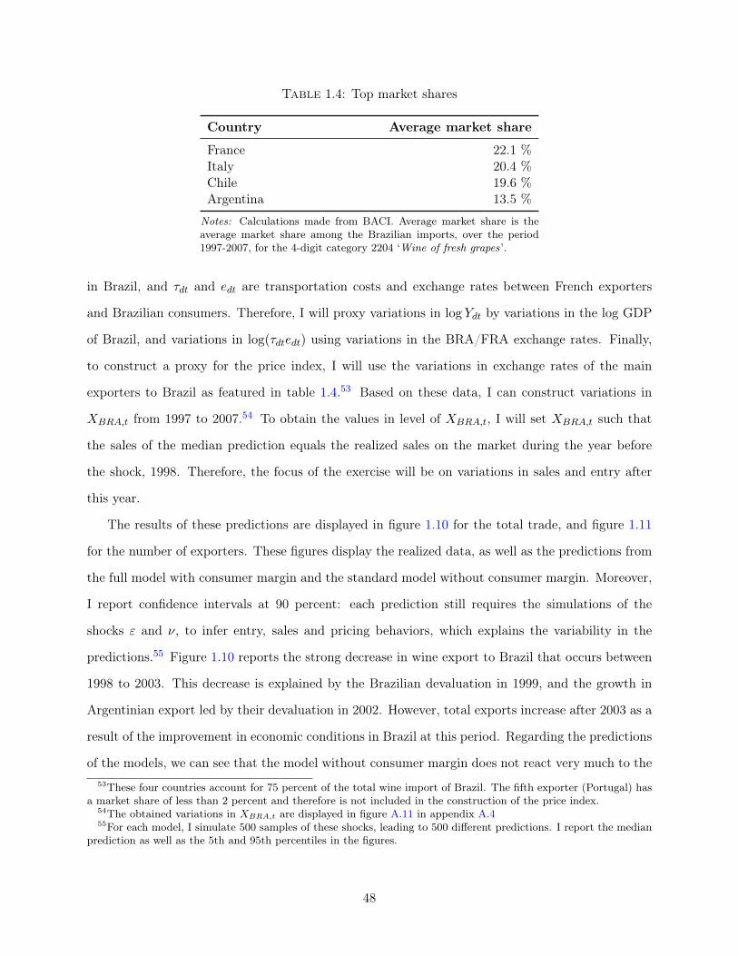
accumulation in explaining firms’ response to shocks. During the sample period, large variations in

exchange rates led to a decrease of the exported values and market shares of French wine on the

Brazilian market.7 Based on these variations in exchange rates that affected the relative price of

French wine, I construct variations in aggregate demand for French wine from Brazilian consumers.

This aggregate demand, in conjunction with outcomes from the model estimated on other desti-

nations, allows me to generate predictions on entry, sales and prices in the Brazilian market, and

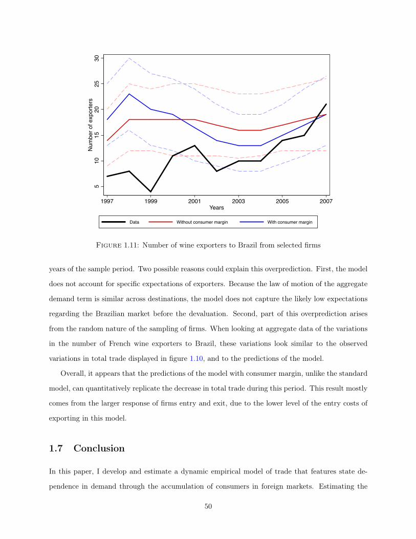
compare them to the actual realizations of these variables. The model with consumer accumulation

is able to replicate, unlike the standard model, the decrease in total trade and in the number of

exporters. The decrease in estimated entry costs between the two models, reduces the option value

of exporting. Therefore, as economic conditions fluctuate, the model with consumer accumulation

(and low entry costs) will predict larger inflows and outflows of exporting firms, and therefore larger

variations in total trade.

This paper is closely related to the literature investigating exporters and firms dynamics. Das,

Roberts, and Tybout (2007) is the first study to quantify entry and per-period fixed costs of export-

ing by estimating an entry model of trade. Their estimation emphasizes the importance of entry

sunk costs to explain the hysteresis of export decisions.8 My paper builds on their contribution by

capturing this hysteresis through state dependence in demand rather than sunk entry costs, and

demonstrating the importance of this extension for a number of micro and macro-level facts. Many

recent studies have documented and studied the specific dynamics of new exporters. Nguyen (2012),

Albornoz et al. (2012), Berman et al. (2015) and Timoshenko (2015) emphasize the role of demand

uncertainty and experimentations to explain exporters dynamics, while Rauch and Watson (2003)7The Brazilian devaluation in 1999 and the depreciation of the Argentinian peso in 2002, that fostered Argentina

exports to Brazil, have increased the relative price of French wines.8Lincoln and McCallum (2015) similarly shows the prevalence of entry costs when estimating fixed costs of ex-

porting for US firms.

5

and Aeberhardt et al. (2014) develop models where exporters need to match with foreign customers

in order to trade. Foster et al. (2016) and Fitzgerald et al. (2016) introduce consumer accumulation

to explain the post-entry growth of firms in domestic and foreign markets respectively.9 However,

they do not study the participation decision in these markets. Similar to my paper, Eaton et al.

(2014) also develop an entry model with accumulation of customers: they use an importer-exporter

matched dataset to estimate an empirical model in which exporters grow through the search of for-

eign distributors and the learning of their own ability.10 However, while they do not allow for other

margins of firms’ growth on foreign markets, my model will feature other sources of time-varying

heterogeneity at the firm level, such as productivity and product appeal. Therefore, I am able to

investigate the importance of this new margin on exporters’ dynamics, and its consequences on the

estimation of trade costs and the predictions of aggregate trade movements.

This article is also related to macroeconomic papers that similarly introduce a consumer margin,

or study aggregate trade dynamics. Arkolakis (2010, 2016) develops a static framework in which a

consumer margin at the firm level generates convex costs of participation to foreign markets and

heterogeneous elasticities of trade in the cross section of firms. I extend this consumer margin to

a dynamic setting to empirically investigate its consequences on exporters’ dynamics. Drozd and

Nosal (2012) and Gourio and Rudanko (2014) show how convex adjustment costs of market shares

can explain several puzzles in international macroeconomics and adjustments of important variables

along the business cycle. Moreover, several recent papers have investigated the reasons for the slow

response to trade, and the discrepancy between short and long-run elasticities of trade.11 This series

of papers develops macroeconomics models to explain this discrepancy between elasticities through

the role of entry and exit of firms, the importance of establishment heterogeneity or the existence of

export-specific investment (Alessandria and Choi, 2007, 2014; Alessandria, Choi, and Ruhl, 2014).

My paper also explains this discrepancy by combining the role of consumer accumulation at the

firm-level, and the entry of new exporters. However, whereas I do not develop a calibrated gen-

eral equilibrium model, I estimate an entry model using micro-data to discipline the role of this

mechanism and investigate its consequences on aggregate trade dynamics.9See also Rodrigue and Tan (2015) that describes demand-side explanations to understand exporters dynamics.

10See also Akhmetova and Mitaritonna (2012) and Li (2014) that show the importance of demand uncertainty, andAw et al. (2011) looking at the impact of R&D activities on exporter decisions.

11See Ruhl (2008) for a review on the discrepancy between trade elasticities in the international macro and inter-national trade literature.

6

Finally, this study heavily builds on the literature related to the estimation of dynamic discrete

choice models (DDCM). These models display a high level of nonlinearity and therefore require the

development of specific techniques to facilitate their estimation. Rust (1987) and Hotz and Miller

(1993) can be cited as seminal papers in the development of these techniques. More specifically, I

employ a MCMC estimator recently developed by Imai et al. (2009) and Norets (2009), that allows

me to account for the existence of persistent unobservables, as well as solve the full solution of the

DDCM.12

The outline of the paper is the following: in the next section, I will present stylized facts about

the trajectories of exporters, that will emphasize the importance of demand in exporters’ dynamics.

In section 1.3, I build an empirical model of export entry that is consistent with these facts. I present

the estimation method in section 1.4, and show the results of the estimation on a set of French wine

makers in 1.5. Finally, section 1.6 will inspect the aggregate implications of the estimated results

through simulations and out-of-sample predictions, and section 1.7 will conclude.

1.2 Stylized facts about exporters dynamics

In this section, I present three important facts about exporters’ dynamics using French customs

data. First, new exporters have low survival rates upon entry, but survival increases quickly with

experience. Second, exported values grow with age in foreign markets, even after controlling for

survival. Third, prices also increase with exporters’ age.

These facts are consistent with the empirical model I will present in the next section: first,

the high level of attrition across age will require the model to account for endogenous selection.

Moreover, the rise in sales, while prices increase on average, indicates that this growth is driven by

a positive shift in the demand schedule of the firm: the consumer margin introduced in the model

will be able to replicate this increase as exporters will start small, and will accumulate consumers

with experience. Finally, the low mark-up charged by young firms to foster this accumulation will

explain the observed increase in prices with age.12An application of this estimation method in Industrial Organization can be found in Osborne (2011).

7

1.2.1 Data

The dataset I used in this paper is provided by the French customs services. These data record

yearly values and quantities exported by French firms from 1995 to 2010.13 Yearly trade flows are

disaggregated at the firm, country and eight-digit product category of the combined nomenclature

(CN). This dataset will be used to present stylized facts about new exporters in this section, and a

restricted sample from the wine industry will be used to conduct the structural estimation described

in the next sections.

I perform a number of procedures to improve the reliability of the data. In particular, I correct

for the existence of a partial-year bias, and improve the reliability of the unit values. The partial-

year bias comes from the mismatch between calendar years and exporting years: because trade data

are based on calendar years, the first year of activity of a new exporter will report lower sales on

average, since this exporter potentially entered anytime during that year.14 These partial years will

imply an overestimation of the growth rate between the first and second year of export. To correct

for this bias, I readjust the dataset using information available at the monthly level. For each new

entry by a firm on a new destination, I readjust the month of entry, and adjust accordingly the

dates of the subsequent exporting flows for that firm. Aggregating this adjusted dataset at the

yearly level, I obtained a transformed dataset that does not display this bias. Second, in order to

improve the reliability of the unit values, I drop all the product categories that use weight as unit

of measure. Even though the weight of a product is sometimes the relevant unit for that product,

it appears that it is used as unit when the type of product in a category is not homogeneous, and

therefore casts some doubt on the use of these quantities to create unit values.15 In addition to

these two important adjustments, Appendix A.1 describes additional procedures implemented on

the dataset to improve its reliability.

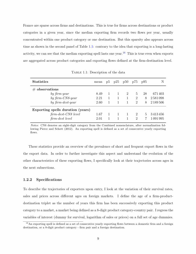
Table 1.1 provides some information on the distributions of the number of observations along

different dimensions. Similarly to what have been documented in the literature, trade flows from13This dataset records most of the exporting and importing flows of Metropolitan French firms: there exists

thresholds under which a firm does not need to report its exporting activity (In 2001 these thresholds were 1,000euros for exports to countries outside of the European union, and 100,000 for the total trade within the EU.)

14See Berthou and Vicard (2015) and Bernard, Massari, Reyes, and Taglioni (2014) for papers investigating theextent and consequences of this bias.

15The main patterns displayed in the next subsection, in particular the one related to prices, appears to hold whenusing the products that use weights as units.

8

France are sparse across firms and destinations. This is true for firms across destinations or product

categories in a given year, since the median exporting firm records two flows per year, usually

concentrated within one product category or one destination. But this sparsity also appears across

time as shown in the second panel of Table 1.1: contrary to the idea that exporting is a long-lasting

activity, we can see that the median exporting spell lasts one year.16 This is true even when exports

are aggregated across product categories and exporting flows defined at the firm-destination level.

Table 1.1: Description of the data

Statistics mean p5 p25 p50 p75 p95 N

# observationsby firm-year 8.49 1 1 2 5 28 671 403by firm-CN8-year 2.21 1 1 1 2 8 2 581 098by firm-dest-year 2.60 1 1 1 2 8 2 189 506

Exporting spells duration (years)firm-dest-CN8 level 1.67 1 1 1 2 5 3 413 456firm-dest level 2.01 1 1 1 2 7 1 091 995

Notes: CN8 denotes an eight-digit category from the Combined nomenclature, after normalization fol-lowing Pierce and Schott (2012). An exporting spell is defined as a set of consecutive yearly exportingflows.

These statistics provide an overview of the prevalence of short and frequent export flows in the

the export data. In order to further investigate this aspect and understand the evolution of the

other characteristics of these exporting flows, I specifically look at their trajectories across ages in

the next subsections.

1.2.2 Specifications

To describe the trajectories of exporters upon entry, I look at the variation of their survival rates,

sales and prices across different ages on foreign markets. I define the age of a firm-product-

destination triplet as the number of years this firm has been successively exporting this product

category to a market, a market being defined as a 8-digit product category-country pair. I regress the

variables of interest (dummy for survival, logarithm of sales or prices) on a full set of age dummies.16An exporting spell is defined as a set of consecutive yearly exporting flows between a domestic firm and a foreign

destination, or a 8-digit product category - firm pair and a foreign destination.

9

The specification will be augmented with fixed effects that will control for the large heterogeneity

that exists across industries, destinations and years. Formally, indexing a firm by f, a destination

by d, a product category by p, and a year by t, the econometric specifications are the following:

Yfpdt =10∑τ=1

δτ1(agefpdt = τ) + µpdt + εfdt, (1.1)

where agefpdt is defined as the number of consecutive years a firm f has been selling the good p to

destination d. Yfpdt will be the logarithm of export sales, the logarithm of prices (unit values),17 or

a dummy equal to one if the firm is still exporting to the market the following year. µpdt will be

a market×year-specific fixed effect such that the variations that identify the coefficients δτ comes

from variations across firms of different ages, within a given destination×product category×year

pair.

Trade data at the firm-product level are known to have a very large level of attrition. These

low levels of survival, especially in the early years of exporting, imply that firms surviving 10 years

differ substantially from firms who recently started to export. Consequently, the variations that

the regressions will capture when comparing old and new firms will mostly come from a selection

effect comparing different set of firms, rather than changes across ages for a given set of firms. In

order to partially account for this dynamic selection, I also present the results when only looking at

firm-product-destination triplets that survive 10 years in their specific markets. Even though this

only partially accounts for selection, since surviving firms are also firms with specific trajectories,

it will show that the observed relationships are not only due to dynamic selection, but also appear

within a constant set of firms.

Another possibility to partially account for this dynamic selection would be to use firm-product

fixed effects, or first difference transformations. These transformations would control for the het-

erogeneity across firms, and only capture variation within a firm-product-destination triplet across

ages. However, the identification of a trend with age is not possible using variations within a given

triplet because the increase of age is a treatment that applies to all firms, and therefore cannot be

separately identified from a cohort effect. I discuss related specifications at the end of the section.17I use the terms unit values and prices interchangeably throughout the paper. As usual with this type of dataset,

prices are obtained by dividing export values by export quantities.

10

1.2.3 Results

Here I present three important facts about exporters, namely the growths of the survival rates,

exported values, and prices with export experience on foreign markets. Regarding the growth

of sales and survival rates, these facts have been extensively documented and discussed in the

literature in international trade and macroeconomics.18 However, I show that these facts still hold

after controlling for the partial-year bias highlighted by Berthou and Vicard (2015) and Bernard,

Massari, Reyes, and Taglioni (2014). Moreover, the increase of prices has not been documented, to

my knowledge, using a comprehensive trade dataset, even though Foster, Haltiwanger, and Syverson

(2016) documents similar patterns for the domestic prices of homogeneous goods, and Macchiavello

(2010) show evidence of similar trajectories for prices of Chilean wine in the UK market.19

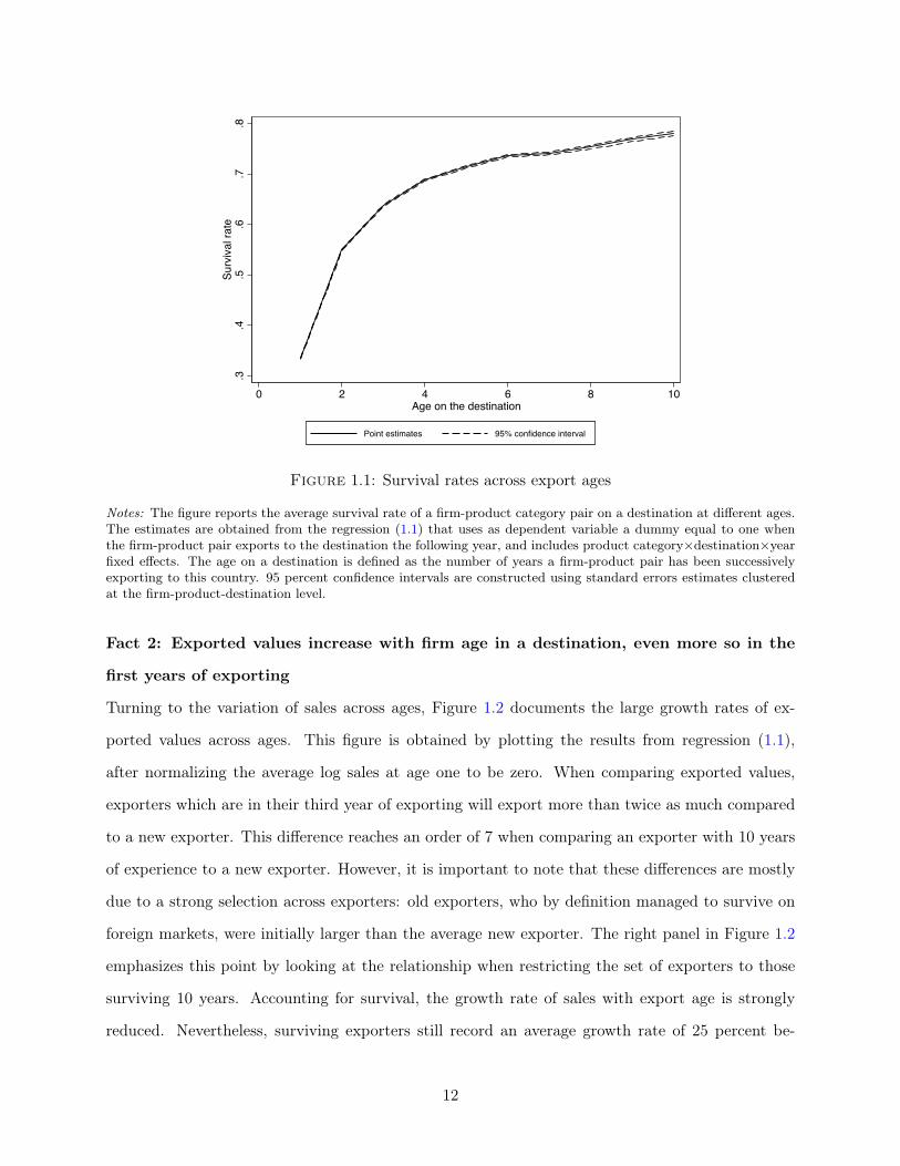
Fact 1: Survival rates are low for new exporters, and strongly increase with their age

First of all, the probability to survive on a market, i.e. to export on this market the following year,

is very low for the average exporter. Figure 1.1 displays the average survival rate for a firm-product

pair on a foreign market, for different age or experience levels. For an exporter in its first year, the

probability to export the following year is roughly 35 percent. However, this survival probability

rapidly increases once exporters have survived several years: this rate is larger than 50 percent at

age 2, and close to 75 percent at age 6. This result reflects the same idea highlighted in the previous

section that most export spells are short lived.

These low, yet increasing, survival rates will have theoretical and methodological consequences.

On the theoretical side, it will be important to have a model of export entry that can replicate and

explain these low survival rates: a model in which entry costs are prevalent will have difficulties

explaining why so many firms exit the export market so rapidly. On the methodological side, these

very low survival rates imply it will be necessary to account for this large attrition when interpreting

differences across firms in a reduced form exercise, and to model this entry decision in the design

of the structural model.18See for instance Ruhl and Willis (2008) for a presentation of these facts and the associated puzzles.19See also Eizenberg and Salvo (2015) which shows evidence of prices cut in the Soda Brazilian market that are

motivated by consumers’ inertia in consumption.

11

.3.4

.5.6

.7.8

Surv

ival

rate

0 2 4 6 8 10Age on the destination

Point estimates 95% confidence interval

Figure 1.1: Survival rates across export ages

Notes: The figure reports the average survival rate of a firm-product category pair on a destination at different ages.The estimates are obtained from the regression (1.1) that uses as dependent variable a dummy equal to one whenthe firm-product pair exports to the destination the following year, and includes product category×destination×yearfixed effects. The age on a destination is defined as the number of years a firm-product pair has been successivelyexporting to this country. 95 percent confidence intervals are constructed using standard errors estimates clusteredat the firm-product-destination level.

Fact 2: Exported values increase with firm age in a destination, even more so in the

first years of exporting

Turning to the variation of sales across ages, Figure 1.2 documents the large growth rates of ex-

ported values across ages. This figure is obtained by plotting the results from regression (1.1),

after normalizing the average log sales at age one to be zero. When comparing exported values,

exporters which are in their third year of exporting will export more than twice as much compared

to a new exporter. This difference reaches an order of 7 when comparing an exporter with 10 years

of experience to a new exporter. However, it is important to note that these differences are mostly

due to a strong selection across exporters: old exporters, who by definition managed to survive on

foreign markets, were initially larger than the average new exporter. The right panel in Figure 1.2

emphasizes this point by looking at the relationship when restricting the set of exporters to those

surviving 10 years. Accounting for survival, the growth rate of sales with export age is strongly

reduced. Nevertheless, surviving exporters still record an average growth rate of 25 percent be-

12

tween ages one and two. Moreover, this growth appears to continue the first six years: at this age,

exporters tend to be on average two times larger compared to their first year of exporting.0

.51

1.5

2Lo

g sa

les


All products

0.5

11.

52

Log

sale

s


Products surviving 10 years


Figure 1.2: Sales across export ages

Notes: The figure reports the cumulative growth of sales, relative to age one, of a firm-product category pair in adestination at different ages. The estimates are obtained from the regression (1.1) that uses logarithm of sales asdependent variable, and includes product category×destination×year fixed effects. The left panel reports the resultsof this regression on the entire sample, while the right panel reports the result from an estimation using only thesample of firms that reach age 10. The age on a destination is defined as the number of years a firm-product pairhas been successively exporting to this country. 95 percent confidence intervals are constructed using standard errorsestimates clustered at the firm-product-destination level.

In conclusion, we observe substantial growth rates of sales during the first years of exports. These

growth rates are large but appear to be lower than previously described in the literature because

of the correction for the partial-year effect highlighted in Berthou and Vicard (2015) and Bernard,

Massari, Reyes, and Taglioni (2014). Moreover, this positive relationship appears to be robust

across product categories and destinations. However, it is important to emphasize that this growth

could be generated by the stochastic nature of the exporting process: by focusing on surviving

firms, we are looking at the “winners” of the exporting game, which could explain unusually large

growth rates. Accounting for this potential mechanism will be one of the roles of the structural

13

model introduced in the next section.

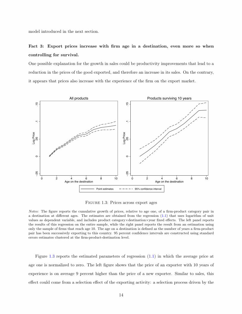
Fact 3: Export prices increase with firm age in a destination, even more so when

controlling for survival.

One possible explanation for the growth in sales could be productivity improvements that lead to a

reduction in the prices of the good exported, and therefore an increase in its sales. On the contrary,

it appears that prices also increase with the experience of the firm on the export market.

-.05

0.0

5.1

.15

Log

Pric

e


All products

-.05

0.0

5.1

.15

Log

Pric

e




Figure 1.3: Prices across export ages

Notes: The figure reports the cumulative growth of prices, relative to age one, of a firm-product category pair ina destination at different ages. The estimates are obtained from the regression (1.1) that uses logarithm of unitvalues as dependent variable, and includes product category×destination×year fixed effects. The left panel reportsthe results of this regression on the entire sample, while the right panel reports the result from an estimation usingonly the sample of firms that reach age 10. The age on a destination is defined as the number of years a firm-productpair has been successively exporting to this country. 95 percent confidence intervals are constructed using standarderrors estimates clustered at the firm-product-destination level.

Figure 1.3 reports the estimated parameters of regression (1.1) in which the average price at

age one is normalized to zero. The left figure shows that the price of an exporter with 10 years of

experience is on average 9 percent higher than the price of a new exporter. Similar to sales, this

effect could come from a selection effect of the exporting activity: a selection process driven by the

14

quality of the product for instance, would imply that older firms which managed to survive, have

higher prices than young exporters. However, when controlling for selection by looking at surviving

firms (Right panel of Figure 1.3), it appears that the growth of prices is even larger compared to

the regression using the full sample: the price after 10 years appears to be in average 12 percent

larger than the price charged by the same firm at age one.

Observing a larger growth of prices when looking at a constant sample of firms has two important

implications. First of all, it means that costs are the main driver of the selection process: high price

firms tend to disappear more in the first years such that the positive correlation between prices and

age is weakened when using the full sample. Second, it implies that this positive correlation cannot

be only driven by dynamic selection. Therefore, an additional mechanism is necessary to explain

why firms tend to increase their price during their exporting life. The structural model presented

in the following section will introduce such a mechanism, through the dynamic pricing of the firms.

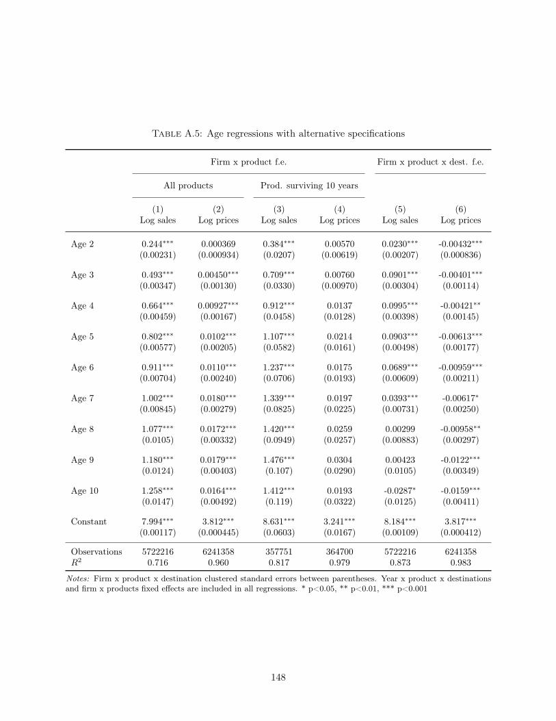
There exists other methods that can partially account for the endogenous selection across ages.

However, within variations cannot be used in this context as it is not possible to separately identify

the role of experience, cohort and trend effects. In appendix A.2, I describe results from two

specifications that use related sources of identification. The first one includes a set of firm-product-

destination fixed effects, such that the identification only comes triplets that exit the market and

reenter a few years later.20 This specification documents a decreasing trend for prices and a hump

shape of sales, which confirms that high price products tend to survive less on average. The second

specification introduces a set of firm-product fixed effects such that the variation is obtained from the

same firm-product pair which is selling to different destinations, with different ages. A potential issue

with this specification comes from the endogenous sorting across destinations: older destinations are

also the ones to which the firm has decided to export first. The results appear consistent with this

mechanism: sales appear to grow faster with this specification, while growth in prices are smaller

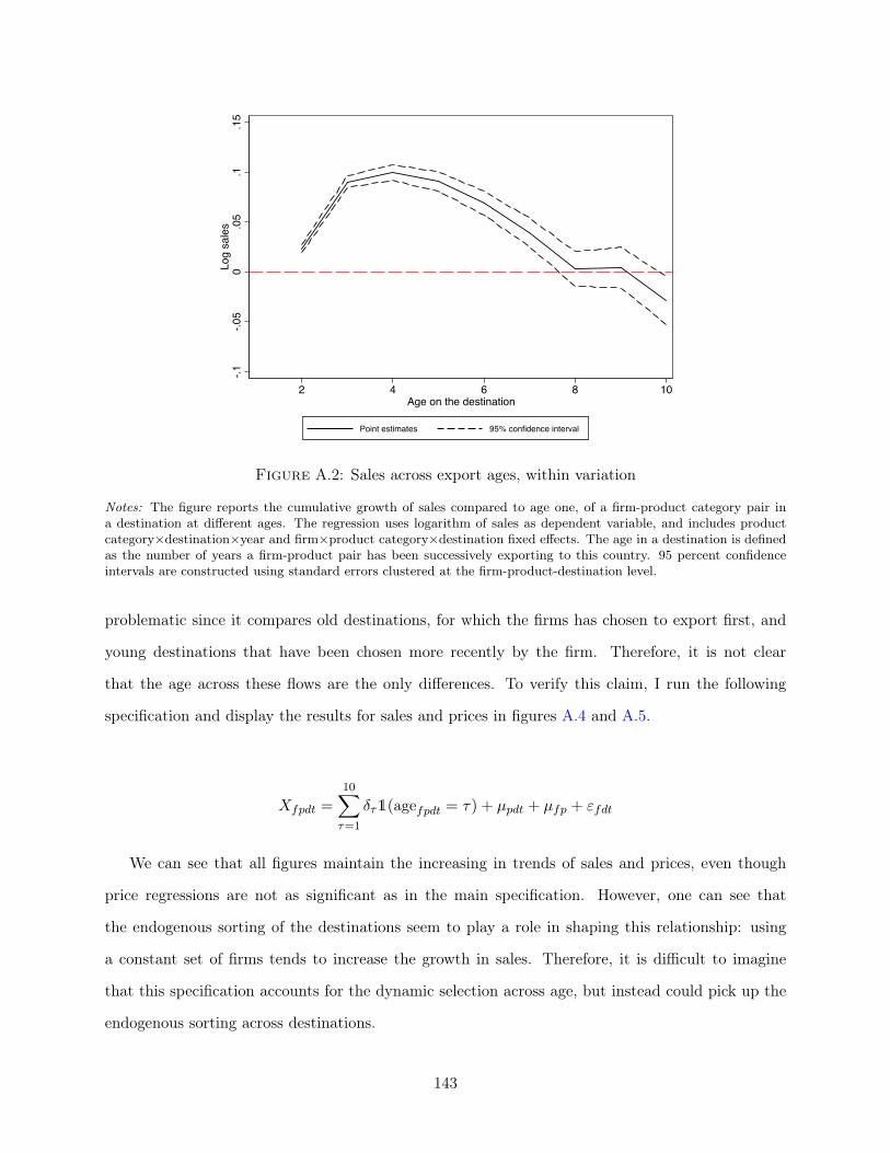
but still positive. Detailed results are provided in appendix A.2.

This section introduced simple facts about exporters’ dynamics that will guide the empirical

model developed below. We can draw three conclusions from these figures. First, survival rates are

very low in export markets and grow with the age of the firm. This result has two consequences: it

implies that the entry decision needs to be accounted for when studying the dynamic problem of the20They are the only triplets that go ‘backward’ in age, and therefore are the only sources of variation.

15

firm. Moreover, this fact is contradictory with a world where the main barrier to export is made of

sunk entry costs: in such a world, exporters would tend to keep exporting once they have overcome

this important barrier. Second, sales of exporters grow rapidly in the first years of exporting. These

large growth rates are also present when accounting for dynamic selection across firms. Third, this

increase in sales is driven by a growth in the demand of the firm: price variations cannot explain this

large increase, implying the importance of demand characteristics as main drivers of this increase in

sales. On the contrary, it appears that prices tend to rise with age, even more so when controlling

for dynamic selection. This pattern could be explained by a dynamic behavior of the firms that

foster their growth in the early years by reducing their prices.

Despite these conclusions, it is difficult to make strong causal statements by comparing firms of

different ages. This brings to light a second benefit of developing and estimating a structural model

to study the entry and growth of exporters: in addition to understanding the dynamic decisions

of firms, it will allow the model to control for the endogenous sorting and attrition of firms, and

recover the different processes that drive the observables variables of the model. The next section

introduces this model.

1.3 Structural model of export entry

This section describes an empirical model of entry into foreign markets in which the accumulation

of consumers creates a new source of dependence in the dynamic problem of the firm. This model

aims to identify the different sources of firms’ profit in foreign markets in order to explain their

export decisions. Therefore, it is crucial to allow for heterogeneity across firms and destinations,

but also to allow this heterogeneity to be persistent over time. Indeed, persistent heterogeneity will

be the main competing hypothesis to sunk entry costs to explain the persistence in export decisions.

As a consequence, this model will feature two additional sources of persistence at the firm level -

productivity and product appeal - and one persistent characteristic specific to destinations - their

aggregate demand. Therefore, a potential profit for a firm-destination pair will depend on four

characteristics: productivity, product appeal, aggregate demand and consumer share.21

21Therefore, I will assume that entry decisions are independent across destinations, once controlling for firms’characteristics, which will keep the state space of the dynamic problem relatively small. McCallum (2015) providessupport for this assumption by finding that entry costs of exporting are mostly country specific. See also Moraleset al. (2014) for a paper that use moments inequalities to maintain such a large state space.

16

The introduction of consumer accumulation will imply two deviations from the standard dynamic

model, which will be consistent with the stylized facts presented earlier: first, firms will start small

in a new market. Their sales and profit will rise in the following years as they accumulate more

consumers. Second, because part of this accumulation of consumers comes from sales, firms will

have dynamic incentives to lower their prices in the first years of exporting to foster their future

demand.

I start by describing the demand schedule of the firm and how the accumulation of consumers

affects the demand from foreign destinations. After introducing the costs associated with the pro-

duction process, I solve the dynamic problem of the firm to study the consequences of this consumer

margin on the entry and pricing decisions.22 In particular, the optimal price charged by the firm

will depart from a constant mark-up over marginal costs to take into account the dynamic impact

of prices on consumer accumulation.

1.3.1 Demand

There exists a wide range of mechanisms that can give rise to inertia in consumption and state

dependence in demand. A large literature in industrial organization has found empirical evidence

of this behavior and have studied their consequences on the market equilibria and the pricing be-

haviors of firms. This literature also points out the large number of mechanisms that can generate

this dependence in demand, as well as the difficulty to empirically disentangle these different chan-

nels. One can cite the existence of habits in consumption, the fact that searching new products is

costly, or the failure of perfect information for the consumers about goods as examples of economic

explanations that leads to state dependence in the demand formed by an agent (see for instance

Dubé, Hitsch, and Rossi (2010) for a paper distinguishing and measuring the contribution of these

different mechanisms).

In order to keep the model tractable, I will introduce state dependence in demand through the

existence of a firm-specific customer base on each destination. This customer base, denoted nfdt,

describes the share of consumers, on a destination d at time t, that includes the product f in its

consideration set. This representation follows the marketing literature that defines a consideration22Note that I do not study the choices made by the firms for each product it could potentially export. Firms are

seen as single-good producers in this model, and will be considered as such in the empirical application using wineproducers.

17

set as the set of products that consumers consider when making purchase decisions.23 It is also

consistent with the idea of customer margin introduced in the macroeconomic and international

trade literature.24 This consumer base is equivalent to introducing some frictions that can explain

that new exporters will start small in foreign markets and will only expand in the subsequent years.

Even though I can specifically identify that these frictions are destination-specific demand frictions,

one could imagine other theoretical foundations for why new exporters face little demand when they

start and slowly grow in export markets.25

Therefore, I will assume that a new exporter has an initial share of consumer n0 when it enters

a new foreign destination. In the subsequent years, the consumer awareness of the products will be

propagated through two mechanisms. First, the sales of a product will increase its awareness in the

next period. Specifically, an euro increase in the sales of a product will increase by η1 the potential

share of consumers in the next period. This acquisition of consumers can arise in a situation in which

consumers have imperfect information about product characteristics, and therefore use sales as a

signal for the expected utility gain obtained from consuming a good.26 Second, another source of

consumer accumulation will come from word-of-mouth: I will assume that each aware consumer will

share its awareness with η2 consumers. Both of these mechanisms will generate a potential growth

in the share of consumers for the firm. However, because some of these reached consumers are

already aware of the existence of the product, this acquisition of new consumers will be discounted

by a factor (1− n′)ψ with ψ > 0, such that the marginal effect of sales s and consumer share n on

the future share n′ is∂n′

∂s= η1(1− n′)ψ,

∂n′

∂n= η2(1− n′)ψ

(1.2)

This specification is largely inspired from the marketing literature as described in Arkolakis (2010):

the accumulation of consumers has decreasing returns such that it is more difficult for an established

firm to accumulate more consumers relatively to a firm with a small initial share. Indeed, for23See for instance Shocker et al. (1991) for an article studying the importance of consideration sets in consumers’

decisions.24See for instance Drozd and Nosal (2012) and Gourio and Rudanko (2014) for macroeconomic papers, and Arkolakis

(2010) in international trade.25For instance, one could think of a Hotelling model in which firms are uncertain about the ideal variety asked by

consumers in a given market, and only comes closer to this variety as they sell and survive on this market.26With CES preferences, the amount spent for a specific good is proportional to the utility gain obtained from the

consumption of this good.

18

established firms, a significant share of these newly reached consumers will already be part of their

consumer share, hence not contributing to its growth. Therefore, the parameter ψ will describe

the importance of these decreasing returns, and the two parameters η1 and η2 will characterize the

importance of the two different sources of growth in the accumulation process.

These two different margins of growth will capture different mechanisms of consumer accumu-

lation, but more importantly will generate different optimal responses by the firm. In a world with

word-of-mouth, where consumers learn from their neighbors, the growth of this consumer share

could be seen as exogenous, only based on the past share of consumers. In this world, firms can-

not affect this accumulation with their pricing decisions.27 However, in a world where consumers

face uncertainty regarding product characteristics and sales are seen as a signal, firms will have

incentives to reduce its price in order to foster the accumulation of consumers. This distinction

between these two sources of growth brings back to the distinction between structural and spurious

structural dependences (Heckman, 1981), that generate different optimal responses by the firm.

Adding an initial condition to these differential equations, n(0, 0) = n, we obtain the following

law of motion for the consumer share of a firm f, at date t and destination d:

nfdt = 1−[(1− n)1−ψ − η1(1− ψ)sfdt−1 − η2(1− ψ)nfdt−1

] 11−ψ (1.3)

Therefore, the share of consumers today nfdt will depend on the sales sfdt−1 and the share of

consumers nfdt−1 in the previous period in this market.

This share of consumer will act as a demand shifter for the firm since it will scale the amount

of demand the firm will receive from each destination. To obtain the total demand of the firm, it

is necessary to solve the consumption problem of the consumers. Because not all consumers know

about all products, consumers will display CES preferences over a limited set of goods. Denoting

Ωi the set of goods in the consideration set of a given consumer i, the utility function is

Ui =

[∫ω∈Ωi

exp

(1

σλ(ω)

)q(ω)

σ−1σ dω

] σσ−1

σ > 1,

27This model does not take into account advertising as a source of growth, even though this could be a naturalcandidate to foster consumer accumulation. The inability to observe this type of expenditures in trade datasets makesit difficult for an empirical model to account for this channel.

19

where q(ω) is the quantity consumed and λ(ω) the appeal of the product. This consumer i will

maximize this utility function given a budget yi devoted to this set of goods, and prices p(ω). As a

solution of this optimization, the quantities qi(ω) demanded by consumer i for a good ω are

qi(ω) =

exp(λ(ω))p(ω)−σP σ−1yi if ω ∈ Ωi

0 if ω 6∈ Ωi

where P is the standard CES price index faced by the representative consumer.28 Aggregating the

demand from individual consumers, we obtain the demand received by the firm f from destination

d at time t:

qfdt = q(λft, Xdt, nfdt, pfdt, εDfdt) = nfdt exp(λft +Xdt + εDfdt)p

−σfdt (1.4)

where Xdt will capture all the aggregate variables of the demand shifter,29 pfdt is the factory price

of the good, and εDfdt is a random demand shock.

It is important to note that the appeal of the product λft does not vary across destinations.

Given the existence of an aggregate demand shifter, this implies that firms cannot vary the relative

quality or appeal of their good across destinations. Therefore, this specification can still explain that

firms will provide different product appeal in different destinations, as long as these differences are

common across firms. This assumption will be fundamental to explain the identification assumption

of the model: while λft and Xdt are respectively firm and destination specific, the customer share

nfdt will be identified through the sales of a firm in a specific destination.

After describing the demand faced by firms, I now turn to the costs associated with production

and international trade.28Note that by having different sets of goods, each consumer would have a different price index. However, I follow

Arkolakis (2010) by assuming that each consumer has probabilistically an equivalent set of goods, such that all

consumers have the same price index defined as P =[∫ω∈Ω

n(ω) exp(λ(ω))p(ω)1−σdω] 1

1−σ

29Xdt ≡ log Ydt − (1 − σ) logPdt + (1 − σ) log(τdtedt) where Ydt ≡ yNdt are total expenditures from a number ofconsumers Ndt, and τdt and edt are respectively iceberg transportation costs and exchange rates that converts thefactory price to the consumer price.

20

1.3.2 Technology and costs

The costs that are associated with production and international trade are similar to those tradi-

tionally assumed in the literature. I first describe the constant marginal costs of production, then

the fixed costs associated with the exporting activity.

First, I assume constant marginal costs of production. These marginal costs are a decreasing

function of the productivity of the firm φft, and will depend on the appeal of the good produced

through a parameter α that characterizes the cost elasticity of appeal. Moreover, I assume the

existence of non-persistent productivity shocks εSfdt, and I allow costs to vary with the destination

market by including a set of coefficients γd. Formally, the marginal cost function of the firm is

cfdt = c(φft, λft, εSfdt) = exp(−φft + αλft + εSfdt + γd) (1.5)

In addition to these production costs, I will assume that firms need to pay entry and per-period

fixed cost for each destination they respectively enter or export to. These fixed costs are defined as

follows

FCd + νfdt =

fd + νfdt if Ifdt−1 = 1

fd + fed + νfdt if Ifdt−1 = 0

where Ifdt is a dummy that equals one if the firm f is active (records positive sales) in destination

d at time t, and νfdt is a random shock on fixed costs. I will assume that this shock νfdt will follow

a logistic distribution with variance parameter σν . The addition of this shock will allow the model

to rationalize all observed decisions made by the firms. Moreover, it is important to note that the

amplitude of these fixed costs will vary across destinations. However, I will restrict this variation

in the estimation, by allocating each foreign destination to specific groups sharing the same value

of fixed costs.30

This achieves the definition of the demand and supply characteristics of the firm. I now turn to

the definition of the profit and value functions associated to the exporting activity of firm.30For instance I will assume that entry and per-period fixed costs will be similar for all European countries. Morales,

Sheu, and Zahler (2014) develop a specific empirical procedure that allows them to flexibly estimate entry and fixedcosts across destinations.

21

1.3.3 Profit and value function

From the demand received by the firm, and the costs associated with production, I derive the

potential profit of the firm for each destination market. After defining the timing of a typical

period, I can define the entry problem of the firm, and the associated value functions. This dynamic

problem will depend on five variables that will define the state space of the problem: the exogenous

variables, that gathers product appeal λ, productivity φ and aggregate demand X, the share of

consumer n, and the presence on the market in the previous year I−1.

In this model, the decisions of the firms are limited. They can decide whether to be active on

the market, and the price they will charge if they decide to export. Consequently, the appeal of the

product, the productivity and the aggregate demand from each destination will be exogenous but

persistent variables that will potentially capture the hysteresis of the exporting decisions. For ease

of exposition, I will denote these variables ξ ≡ (λ, φ,X) such that, ignoring the subscripts and the

parameters of the model, the profit function of a firm is

Π(ξ, n, p, ε, I−1, ν) = q(ξ, n, p, εD)[p− c(ξ, εS)

]− FC(I−1)− ν

= π(ξ, n, p, ε)− FC(I−1)− ν

where I−1 is a dummy equal to one if the firm was selling on the market in the previous year. This

profit function is made of a variable profit and fixed costs. Despite having CES preferences, this

variable profit could be negative because of the dynamic nature of the pricing decision of the firm:

some firms could set a price lower than their marginal costs to foster future demand. The second

part of the profit function comes from the fixed costs of exporting FC(I−1) that will depend on

the past presence of the firm on the market. Finally, the profit shock ν will allow the empirical

model to explain the entry and exit decisions of firms that cannot be rationalized by the values of

the variable profit and fixed costs.

However, this profit will only be obtained by the firm if it decides to be active on the market

at this period. In order to study the problem of the firm, it is necessary to define the timeline of

a typical period, which provides the timing at which decisions are made and the information sets

available to the firms when they make these decisions. Figure 1.4 displays the timeline of a period

22

that defines the dynamic problem of the firm.

Information

DecisionsStart

λ φX n

ν

Entry Mark-up

εS

εD

End

Figure 1.4: Timeline of one period

As described in figure 1.4, the firm observes at the beginning of the period its exogenous variables,

λ, φ, n and X. After realization of the profit shock ν, it decides whether to export in the market. If

the firm decides to export, it optimally chooses the mark-up to charge over their marginal costs.31

Finally, sales and prices will be obtained after observing the realization of the non-persistent shocks

ε.32

Therefore, denoting µ the multiplicative mark-up of the firm such that p = µc, the value function

of the firm can be defined as the following:

V (ξ, n, I−1) = EνmaxVI(ξ, n)− FC(I−1)− ν ; VO(ξ)

with VI(ξ, n) = max

µ

Eε

π(ξ, n, µ, ε) + βEV ′(ξ, n′(ξ, n, ε, µ), 1)

,

VO(ξ) = βEV ′(ξ, n0, 0),

EV ′(ξ, n′, I) =

∫ξ′V (ξ′, n′, I) dF (ξ′|ξ).

The first line describes the entry problem, in which the firm chooses between exporting VI(ξ, n)−

FC(I−1) and inactive VO(ξ). By being inactive, the firm makes no profit today but retains the

possibility to update its decision in the next period. In contrast, when exporting, it obtains a

present profit that will depend on the shocks ε and the mark-up chosen by the firm. Moreover, the

firm will have a continuation value, EV ′(ξ, n′(ξ, n, ε, µ), 1), characterized by a stock of consumer n’31Choosing the mark-up rather the price facilitates the computation of the solution, while allowing for structural

shocks ε in demand and costs.32The assumptions made regarding the timing of the shocks and decisions are mostly driven by the construction

of the empirical model. The realization of the shock ν before the entry decisions allow the model to rationalize entrydecisions that couldn’t be explained otherwise. Similarly, the realizations of the shocks ε after the markup decisionsgenerate structural errors in the sales and prices equations that can explain sales and prices variations.

23

and lower fixed costs to pay in the next period. This continuation value will be constructed from

the transition of the exogenous variables F (ξ′|ξ), and the expected value of V (ξ, n′, I).

In order to solve this problem, it is necessary to proceed through backward induction by de-

scribing the pricing decision made by the firm once it enters. This optimal pricing decision leads to

the expected profit of the firm, and therefore solves for the entry decisions. I describe these optimal

decisions and the value functions of the problem in the next subsection.

1.3.4 Firms’ decisions: entry and pricing.

After defining the problem of the firm, I can now derive the optimal entry and pricing decisions of

the firm. Because the accumulation of consumers is based on the sales of the firm, the optimal price

charged by the firm will deviate from a standard constant mark-up. Instead, firms will optimally

reduce their mark-up to account for the accumulation of consumers. Because this pricing decision is

taken once the firm has decided to enter, I start by describing the optimal mark-up charged by the

firm. By backward induction, I will infer the expected profit of the firm conditional on this optimal

pricing decision, and therefore infer the value and probability of exporting.

Optimal price The choice of the mark-up of the firm involves solving a dynamic problem: by

affecting the sales of the firm today, the price charged by the firm affects the share of consumers to-

morrow. Therefore, the firm will have incentives to reduce its price today to foster the accumulation

of future consumers.

The choice of mark-up of the firm is made after entry, in order to maximize the sum of the present

profit and the continuation value of exporting. Formally, the problem and first-order conditions are

the following:

VI(ξ, n) = maxµ

Eε

π(ξ, n, µ, ε) + βEV ′(ξ, n′(ξ, n, ε, µ), 1)

=⇒ Eε

∂π(ξ, n, µ, ε)

∂µ+ β

∂n′

∂µ

∂EV ′(ξ, n′, 1)

∂n′

= 0

24

Therefore, the optimal price of the firm is:

p(ξ, n) = µ(ξ, n)c(ξ, n) (1.6)

with µ(ξ, n) =σ

σ − 1

1

1 + βEw(ε)η1(1− n′)ψ ∂EV′(ξ,n′,1)∂n′

The optimal mark-up charged by the firm has two components. First, the firm will apply the

standard CES mark-up σσ−1 based on the price-elasticity of the demand. Second, the firm will

apply a discount factor based on the dynamic incentives it has to lower its price to attract more

consumers in the future. This factor will depend on two elements: first, how much this increase in

sales will increase its consumer share tomorrow, η1(1−n′)ψ; this element will induce lower mark-ups

for small or young firms that benefit from higher returns of accumulation. Second, the extent of

this discount will also depend on the impact of this increase in the future consumer share on the

continuation value ∂EV ′(ξ,n′,1)∂n′ . This effect will not be linear but hump shaped with the profitability

of the firm:33 young firms that are unlikely to survive will not have incentives to invest in future

consumers. Firms that can use extra consumers to increase their probability of survival will get

the largest benefits from increasing their consumer share. However, because of the concavity of

the value function conditional on surviving, this effect will be smaller for high profit firms that are

likely to survive in the next period. Finally, note that this equation defines the unique optimal price

charged by the firm but only through an implicit function, since the future share n’ will depend on

the price charged.34

Consequently, the accumulation of consumers will imply heterogeneous mark-ups by the firms,

depending on their current share of consumers, and their expectations on future profits. Having33This comes directly from the probability of exit that makes the value function of the firms increasing and convex

for low profitability firms, and increasing and concave for higher profit firms.34Note that

Ew(ε)

η1(1− n′)ψ ∂EV

′(ξ, n′, 1)

∂n′

≡∫ε

c(ξ, ε)q(ξ, n, µ, ε)∫εc(ξ, ε)q(ξ, n, µ, ε)

η1(1− n′)ψ ∂EV′(ξ, n′, 1)

∂n′dF (ε)

To overcome the absence of closed form solution for the optimal price, I will use a grid to solve the optimal price ofthe firm in the estimation procedure. Moreover, solving the dynamic problem of the firm will also be facilitated byassuming that EεEV ′(ξ, n′(ξ, n, ε, µ), 1) = EV ′(ξ, n′(ξ, n, Eεε, µ), 1). This assumption will allow me to redefine theproblem such that

VI(ξ, n) = maxµ

Eεπ(ξ, n, µ, ε) + βEV ′(ξ, n′(ξ, n, ε, µ), 1)

= max

µ

Eεπ(ξ, n, µ, ε) + βEV ′(ξ, n′(ξ, n, µ), 1)

for which Eεπ(ξ, n, µ, ε) admits a closed-form solution that will facilitate the evaluation of the model.

25

described the optimal mark-up of the firm, it is possible to infer the expected profit of the firm in

case of entry. Therefore, I can evaluate the two options of the firm, and study its entry decision.

Entry condition Knowing the expected option values of being active or inactive, I can now study

the entry decision of the firm. The firm will pick the most profitable option, after observing the

shock ν that affects the fixed costs of being active on a market. The logistic assumption for this

shock will generate a closed-form solution for the probability of entry, but also for the expected value

function before observing this shock. Formally, the expected value of the firm before observing the

shock ν is

V (ξ, n, I−1) = EνmaxVI(ξ, n)− FC(I−1)− ν ; VO(ξ)

= σν log

[exp

(1

σν

(VI(ξ, n)− FC(I−1)

))+ exp

(1

σνVO(ξ)

)].

This equation closes the dynamic problem of the firm, by providing the fixed point that defines the

value function V (ξ, n, I−1). Moreover, the probability for a firm to be active, before the realization

of the fixed cost shock ν, is,

P (I = 1|ξ, n, I−1) =1

1 + exp(− 1σν

(DV (ξ, n)− FC(I−1))) (1.7)

with DV (ξ, n) = VI(ξ, n) − VO(ξ). This last equation predicts the probability of entry of a firm,

conditional on its current characteristics, described by ξ, n and I−1. While n and I−1 are en-

dogenous, ξ are exogenous and unobservables variables. Therefore, to finish the derivation of the

model, it is necessary to describe the evolutions of these exogenous variables across time. These

evolutions will be important to compute the expectation of the value functions, EV ′(ξ, n, I−1), as

well as disciplining the variations of sales and prices across times in the empirical application.

1.3.5 Evolution of exogenous variables

In order to close the definition of the dynamic problem of the firm, I need to specify the evolution

of the exogenous variables of the model. These exogenous variables will be important as they can

account for a large amount of the persistence in export decisions observed in the data. Most of

26

the hysteresis in exporting decisions is likely to come from the persistence over time of fundamental

characteristics of the firm such as productivity or product appeal. Therefore, it is necessary to allow

these processes to be persistent. Moreover, to account for the important attrition rate across ages,

it is also necessary to let these processes vary across time, through random shocks. Consequently,

one wants to assume general processes that are time variant, and allow for important persistence

in their evolution. For these reasons, I will assume that these three variables will follow AR(1)

processes, with flexible parameters. Formally, I assume

λft = ρλλft−1 + σλελft

φft = µφ + ρφφft−1 + σφεφft

Xdt = µXd + ρXXdt−1 + σXεXdt

(1.8)

where the ε shocks follow a normal distribution with zero mean and unit variance. Note that, by

normalization, λ is centered around zero: since both X and λ enters linearly in the demand function,

it is not possible to separately identify their respective means. Moreover, because Xdt describes the

aggregate demand from a destination d, I allow the mean µXd of this process to change across

destination. This will allow the model to capture different trends in aggregate demand across

different destinations.

Finally, I need to impose distributional assumptions on the initial conditions of these unobserv-

ables. I assume that the distributions of product appeal and productivity are stable over time such

that the initial distributions are constrained by a stationary assumption. Consequently, we have

λf0 ∼ N

0,σλ√

(1− ρ2λ)

φf0 ∼ N

µφ1− ρφ

,σφ√

(1− ρ2φ)

(1.9)

However, I will assume that the variation in aggregate demand across destinations does not arise

from a stationary distribution. Therefore, I will assume a flexible distribution of initial conditions

for Xd0 such as

Xd0 ∼ N(µX0 , σX0). (1.10)

27

Moreover, I will assume that the initial share of consumers, which will apply to firms that records

positive sales the year before the beginning of the model, follow a Beta distribution with parameters

1 and 5.35

This concludes the derivation of the model. Each firm observes exogenous variations in its

export profitability through variation in its productivity, product appeal and the demand in each

destination. Based on these variations, the firm decides to enter or exit various destinations where

it decides at which prices to sell its good. The more the firm sells on a market, the more consumers

will be ready to buy from it in the next period, fostering its demand and profit in the next period.

After describing the model, I now describe the restrictions I impose to obtain a model without

consumer accumulation, that will behave similarly to standard models used in the literature.

1.3.6 Restricted model

In order to assess the importance of consumer accumulation on estimated trade costs and aggregate

response to trade, I will estimate a restricted version of the model that does not feature this

mechanism. This restricted model is equivalent to assuming that exporters will have a consumer

share nfdt equal to one when they are active on the market. As a consequence, firms will not have

incentives to deviate from the CES pricing, and the mark-ups will be similar across all firms.

This restricted version of the model can be seen as the canonical model used in the literature. In

this model, firm-level heterogeneity and entry costs of exporting explain the hysteresis in exporting.

This model can be seen as a dynamic version of Melitz (2003), as estimated by Das, Roberts, and

Tybout (2007). Estimating this restricted model will be essential to assess the importance of the

accumulation of consumers on the outcomes of the estimation and the aggregate implications of the

model.

1.4 Estimation

In this section, I describe the procedure used to estimate the parameters of the model. The likelihood

is directly obtained from the three structural equations of the model. However, the evaluation of35Given the number of firms in this case, and the length of the panel I will use (14 periods), this assumption has

no consequence on the estimation.

28

this likelihood is made cumbersome by the number of persistent and unobservables variables and

the dynamic problem of the firm.

I start by describing the likelihood of the problem, based on the three structural equations

linked with the observable variables (sales, prices and participation to export). I then turn to the

algorithm to show the advantages of a MCMC estimator to facilitate the estimation of the model.

Finally, I provide the intuition behind the identification of the parameters and unobservables of the

model.

1.4.1 Likelihood

I start by presenting the likelihood that is obtained from the three main equations of the model:

the demand equation in which the stock of consumers of the firm appears, the pricing equation that

features the dynamic mark-up charged by the firm, and the entry probability that describes the

exporting decision on each destination.

First of all, the demand and price equations (1.4), (1.5) and (1.6) are taken in logarithm to

obtain

log sfdt = log nfdt + λft +Xdt + (1− σ) log pfdt + εDfdt

log pfdt = −φft + αλft + logµ(ξ, nfdt) + γd + εSfdt

This block will constitute the first part of the likelihood. Assuming that ε follows a bivariate normal

distribution with variance Σ, I define this likelihood block as Lε(sfdt, pfdt|ξfdt, nfdt; Θ),36 with Θ

being the full set of parameters, such that

Lε(sfdt, pfdt|ξfdt, nfdt; Θ) = GΣ

(log sfdt − log nfdt − λft −Xdt − (1− σ) log pfdt ;

log pfdt + φft − αλft − logµ(ξ, n)− γd) (1.11)

where GΣ is the density function of a bivariate normal distribution with means zero and variance

matrix Σ.

The second block of the likelihood will be based on the entry decision of the firm. Equation36As previously defined, ξfdt gathers all the exogenous variables of the model - product appeal, productivity and

aggregate demand - such that ξfdt ≡ λft, φft, Xdt

29

(1.7) defines the probability to enter for a firm, based on its set of unobservables ξ, its stock of

consumer n and its past exporting activity. I denote this function Lν(Ifdt|ξfdt, nfdt, Ifdt−1; Θ) that

is obtained from the binary choice made by the firm

Lν(Ifdt|ξfdt, nfdt, Ifdt−1; Θ) =

[1 + exp

(−DV (ξfdt, nfdt) + FC(Ifdt−1)

σν

)]−Ifdt×[1 + exp

(DV (ξfdt, nfdt)− FC(Ifdt−1)

σν

)]Ifdt−1(1.12)

where function DV (ξfdt, nfdt) and FC(Ifdt−1) are defined as previously. Therefore the total likeli-

hood for a given observation Dfdt ≡ sfdt, pfdt, Ifdt is

L(Dfdt|Dfdt−1, ξfdt, nfdt−1; Θ) = Lν(Ifdt|ξfdt, nfdt, Ifdt−1; Θ)× Lε(sfdt, pfdt|ξfdt, nfdt; Θ).

To obtain the unconditional likelihood, that does not depend on the unobservables of the model, it

is necessary to integrate out this set of unobservables. However, because these unobservables are

persistent over time, the likelihood of the entire dataset D is obtained by repeatedly integrating the

unobservables from period T to 0. Formally, the full likelihood is

L(D|D−1; Θ) =

∫n−1

∫ξ0

...

∫ξT

∏f,d

L(DfdT |DfdT−1, ξfdT ; Θ)× ...× L(Dfd0|Dfd−1, ξfd0, nfd−1; Θ)

dF (ξfdT |ξfdT−1)× ...× dF (ξfd0) dF (nfd−1)

where F (ξfd0) is defined by the density of the initial unobservables defined in equations (1.9) and

(1.10), and F (nfd−1) the beta distribution assumed for firms that were exporting the year before the

beginning of the estimation sample, and Dfd−1 the observables previous to the estimation sample.

After describing the likelihood of the problem, I now turn to the estimation procedure by describing

the algorithm aiming to find the posterior distribution of parameters Θ.

1.4.2 Algorithm

To estimate the model, I develop a Markov Chain Monte Carlo (MCMC) estimator to account

for two important difficulties in evaluating the likelihood of this problem: the different sources of

persistent and unobservable heterogeneity and the dynamic problem of the firm. First, the persistent

30

unobservable characteristics make it necessary to perform a large number of integration in order to

evaluate the likelihood. This is particularly cumbersome given the persistent nature of these sources

of heterogeneity. The second difficulty comes from the need to solve for the value functions in order

to obtain the objects DV () and µ() and evaluate the likelihood. The literature on dynamic discrete

choices model, starting from Rust (1987) is mostly devoted to this specific problem, which requires

obtaining the solution of the Bellman equation through value function iterations until reaching a

fixed point.37 Therefore, even in the absence of unobservables, the likelihood function is a highly

non-linear function of the parameter set Θ, increasing the difficulty, and the computing time, of

evaluating the likelihood.

In order to circumvent these difficulties, I employ a MCMC estimator, taking advantage of recent

Bayesian techniques to sample the posterior distribution of the parameter Θ, conditional on the data.

The choice of a Bayesian estimator relies on two recent findings from the Bayesian econometrics

literature. First, Arellano and Bonhomme (2009) show how Bayesian hierarchical models nest fixed

and random effects models: using a prior distribution of the unobservable of the model, the posterior

distribution of the unobservable term will be very precise when many observations are available (for

instance when one firm sells to many destinations), such that this posterior distribution will be

close to the fixed effects value. When the number of observations is limited (for instance when a

firm only sells to one country), the prior distribution of the unobservable variable, as specified by

the model, will constrain the value of this variable similar to the random-effect case. Moreover,

using MCMC in this context will allow one to perform the integration by updating unobservables as

latent variables of the model. Therefore, a Bayesian estimator offers a attractive way of integrating

these unobservables, while correcting for the first-order bias that exists in fixed and random-effects

models.38

Second, to overcome the computational burden of solving the value functions in the likelihood,

Imai, Jain, and Ching (2009) and Norets (2009) show how to take advantage of the iterative feature

of the MCMC estimator, by only updating the value functions in the Bellman equation once at each37This problem can be largely simplified using the mapping between conditional choice probabilities and value

functions, as highlighted in Hotz and Miller (1993). However, in my application where state variables are mostlyunobserved, obtaining conditional choice probabilities in a first step is not trivial, and likely to be an impreciseexercise.

38Roberts, Xu, Fan, and Zhang (2012) also use this type of estimator in a similar context. The main differencebeing that the unobservables terms are time-invariant in their model while they vary in mine, making the integrationissue even more stringent in my setup.

31

iteration. The intuition is that there is no need to fully solve for the fixed point of the value function

at each point of the parameter set. Instead, it is possible to only iterate the Bellman equations a

limited number of times at each iteration of the Markov chain, reusing these value functions as initial

values for the next iteration. As the Markov chain converges and explores the posterior distribution

of Θ, the value function will also converge toward the fixed point that solves the Bellman equation.

Overall, the MCMC estimator will explore the posterior distribution of the parameters Θ. This

distribution is proportional to the product of the likelihood and the prior distribution such that

P (Θ |D) ∝∫ξL(D | ξ,Θ) dF (ξ |Θ)P (Θ) (1.13)

where L(D |Θ) =∫ξ L(D | ξ,Θ) dF (ξ |Θ) is the likelihood of the problem and P (Θ) is the prior

distribution of the parameter set. Because I do not want these priors to influence the posterior

distribution of the parameters, I will assume that all the priors are flat, except for values of pa-

rameters that do not satisfy theoretical or stationarity constraints.39 Therefore, the goal of the

Markov Chain is to repeatedly sample from the posterior distribution according to (1.13). This will

be achieved by alternatively sampling parameters conditional on unobservables, and parameters

conditional on unobservables. In this specific application, an iteration in the Markov chain consists

of three different steps, summarized in the following iteration.

At an iteration s, the inputs of the Markov chain are Θ(s), ξ(s) and the history of value functionsV (Θ(h))

sh=s−m and their associated parameters sets

Θ(h)

sh=s−m for a given m ≥ 0. The steps

of a typical iteration are:

• Sample ξ(s+1) proportionally to L(D|ξ,Θ(s))f(ξ|Θ(s))

• Sample Θ(s+1) proportionally to L(D|ξ(s+1),Θ)f(ξ(s+1)|Θ)P (Θ)

• UpdateV (Θ(h)),Θ(h)

s+1

h=s+1−m using Θ(s+1) and V (Θ(s+1)).

Two important points are worth noticing regarding this algorithm. First, the large size of the

parameter space requires updating the parameters sequentially rather than simultaneously. In total,39I exclude from the support of Θ (or equivalently assigned a prior probability of zero for these values), negative

values for the variance parameters, as well as values beyond -1 and 1 for the autocorrelation parameters. Finally, Ialso impose the average fixed cost and entry cost parameters (f , fe) to be positive. and the parameter ψ to be largerthan zero.

32

30 parameters will be estimated in the model. Consequently, a Gibbs sampling is used in which

different parameters blocks are created and sequentially updated based on the different blocks of

the likelihood.40 Second, the value functions that allow the computation of the objects DV (.) and

µ(.) will be obtained on a grid that will be updated throughout the algorithm. The specific values

of DV (.) and µ(.) will then be obtained by interpolation to be evaluated at any point in the state

space. I provide extensive details in appendix A.3 about the implementation of the algorithm.

Due to the complexity of the estimation procedure, two parameters will not be estimated and

set to specific values from the literature. First of all, I do not estimate the value of β, the discount

rate of future periods. This parameter is difficult to identify in dynamic discrete choice models

and I therefore set its value to 0.9, following Das, Roberts, and Tybout (2007).41 Second, I do not

estimate the elasticity of substitution of the CES utility function. Estimating the price-elasticity of

demand using trade data is not trivial given the absence of product characteristics, which implies

unobserved vertical differentiation across goods.42 Therefore, I will use the value obtained by Broda

and Weinstein (2006) for the corresponding industry; they estimate an elasticity of 2.2 for the wine

industry, which I will utilize and keep constant throughout the algorithm.

After describing the details of the estimation procedure, I provide, in the next section, intuition

about the sources of identification of the parameters and the unobservables.

1.4.3 Identification intuition

Despite the complexity of the algorithm, estimating this model using micro data and a full in-

formation estimator provides simple intuitions of the identification of the parameters. Moreover,

the alternative sampling of unobservables and parameters shed light on the separate sources of

identifications of each component of the likelihood.

To describe the sources of identification, it is important to distinguish the identification of un-

observables and parameters. Let’s assume first that the parameters of the model are known. In

this situation, the identification of the unobservables mostly come from a variance decomposition40Despite the separation of the parameters in different sets, the existence of value functions in the likelihood creates

a dependence between most parameters of the parameter set and the different part of the posterior distribution.Therefore, Metropolis-Hastings algorithms are used to sequentially update these different blocks.

41Magnac and Thesmar (2002) provides an extensive discussion of identification issues in DDCM.42See Piveteau and Smagghue (2015) for a discussion on the estimation of this elasticity. In theory, prices in other

destinations could be used as instrument for the prices. However, this requires controlling for the impact of qualityon marginal costs, which is part of the model (through the parameter α).

33

of the demand shifters and prices. Indeed, knowing sales and prices, the demand shifter is decom-

posed between a firm-year component (the product appeal λft), a destination-year component (the

aggregate demand Xft), and a firm-destination-year component (the consumer base nfdt). Once

the product appeal is known, the productivity φft is identified by price variations across firms.

Therefore, the identification of the unobservables mostly comes from a decomposition of observ-

ables variables, which is straightforward once the parameters of the model are known. Moreover,

the hierarchical structure and the entry decisions will bring additional information to identify the

posterior distribution of these unobservables. For instance, if a firm is not exporting one year, the

information from previous and future years will help identify the potential value of the unobserv-

ables. Similarly, the entry decisions in foreign destinations will bring additional information about

the posterior distribution of these unobservables: if a firm only exports to one destination at a given

year, the fact that it does not export somewhere else will provide information regarding the latent

value of its product appeal or productivity.

Let’s now turn to the identification of the parameters of the model, assuming that the unob-

servables are known. The 30 estimated parameters can be divided in three groups: 17 of them are

related to the laws of motion of the unobservables, 6 to the demand and supply equations, and 7

related to the dynamic problem of the firm. Knowing the unobservables of the problem, the iden-

tification of the parameters that describes their distribution and law of motions is straightforward.

Regarding the parameters that are linked to the demand and pricing functions, their identification

is similar to a regression of prices on destination dummies and the appeal of the product, while the

parameters of the variance matrix are obtained from the variance of the unexplained variation in

prices and sales. Finally, the parameters related to the entry problem of the firm are obtained by

comparing potential profits and firms’ observed decisions. Based on the characteristics of the firms

and destinations, the laws of motion of unobservables, and the parameters of the cost and demand

functions, it is possible to construct the potential profit of each firm on each market. Based on these

potential profits, the number of exporters will identify the per-period fixed costs, the persistence

in exporting the entry costs, and the remaining variance in exporting decisions will identify the

required variance of these fixed costs’ shocks.

Consequently, the identification of the unobservables conditional to the parameters, and of the

unobservables conditional to the unobservables are quite straightforward. The goal of the MCMC

34

estimator is to repeatedly sample each component conditional to the other, in order to obtain their

joint distribution. After a necessary period of convergence, the Markov Chain will describe the

posterior distributions of the parameters.

1.5 Results

I implement my estimation on a set of wine exporters from France; the choice of the industry is

based on two criteria. First, wine producers only export wine. Therefore, it is reasonable to assume

that the entry decisions on foreign destinations are made at the firm level, and it is possible to

aggregate sales and prices at the level of the firm for each destination. Second, the wine industry

is a large industry in France and, therefore, I can obtain a large enough sample of exporters with a

relatively extended set of destinations. In appendix A.1.2, I describe the specific selection procedure

to obtain the estimation sample of 200 firms, and provide statistics to describe this sample.

In order to describe the results of the estimation, I start by describing the fit of the model

relative to the exporters’ dynamics presented earlier. Then I will present the estimated values of

the parameters, and in particular the decrease in entry costs induced by the introduction of the

consumer margin. Finally, I will describe the evolution of the consumer margin and the mark-ups

charged by firms at different export ages.

1.5.1 Fit of the model

I report in this section the fit of the model regarding the survival rates, sales and prices of the

firm-destination pair at different ages. Figure 1.5 reports the predictions of the model relative to

the data. I also report the results of the restricted version of the model, which does not contain a

consumer margin.

As reported in figure 1.5, the full model with consumer accumulation can reproduce most of

the growth in sales across ages (top left figure). The ability of the model to capture this growth

explains how the model can perform better in terms of survival rates (top right figure): as a firm

accumulates more consumers in a foreign destination, raising its sales, it also increases its future

profit, and therefore its survival rate. However, this growth in sales is not sufficient to fully explain

the low survival rates of young exporters, and, therefore, does not entirely solve the puzzle linked

35

8.5

99.

510

Log

sale

s


.6.7

.8.9

Surv

ival

rate

s


1.8

1.9

22.

12.

2Lo

g pr

ice


1.5

1.6

1.7

1.8

1.9

Log

pric

e (fi

rms

surv

ivin

g 10

y.)


Data Full model Restricted model

Figure 1.5: Predictions of survival rates, sales and prices across ages.

with young exporters dynamics. In comparison, the restricted model cannot explain this rise in

sales and even less in survival rates: in the restricted model, the predicted survival rate is constant

across ages, between 75 and 80 percent, which is similar to the average survival rate in the sample.

However, the predictions on prices appear quite similar across models (bottom figures). Both of

them can reproduce the decrease in prices with age. When looking at firms surviving 10 years, we

can see that the full model can do slightly better in explaining the rise in price with the age of the

firm. Therefore, the heterogeneous mark-ups obtained from the dynamic problem of the firm seems

to help the model in predicting low prices at young ages.

After describing the fit of the model, I turn to the description of the estimated values of the

36

parameters.

1.5.2 Estimated parameters

The results of the estimation of the model are reported in table 1.2. I report for each parameter

the mean of its posterior distribution, as well as its 90 percent confidence interval.

Table 1.2: Estimated parameters

Parameter Estimate 90% Confidence Interval

Lower bound Upper bound

Per-period fixed costs Europe 7 994 6 761 9 194(in 2000 euros) Americas 7 495 6 693 8 304

Asia/Oceania 8 019 7 080 8 930

Entry fixed costs Europe 33 730 30 303 37 078(in 2000 euros) Americas 23 656 21 092 26 208

Asia/Oceania 28 619 25 387 31 928

Variance of entry shocks σν 9 656 8 589 10 620

Law of motion of n n0 0.033 0.031 0.034n 0.015 0.014 0.016η1(10−5) 0.12 0.11 0.14η2 0.27 0.23 0.29ψ 0.44 0.00 0.93

Law of motion of appeal ρλ 0.98 0.98 0.98σλ 0.19 0.18 0.20

Law of motion of productivity ρψ 0.93 0.91 0.94σψ 0.09 0.08 0.09µψ -0.12 -0.14 -0.10

Law of motion of agg. demand ρX 0.93 0.93 0.94σX 0.09 0.09 0.09µX1 0.98 0.91 1.03µX2 0.88 0.74 0.97µX3 0.89 0.77 0.97µX0 14.58 14.31 14.83σX0 0.46 0.32 0.65

Elasticity cost of appeal α 0.73 0.73 0.74

Cost dummies γ2 0.38 0.36 0.39γ3 0.30 0.29 0.30

Variance matrix Σ11 1.25 1.25 1.26Σ12 0.17 0.17 0.17Σ22 0.56 0.54 0.57

First, looking at the law of motion of the consumer margin, we note that the initial share of

37

consumers at entry (n0) is relatively small, equal to 3 percent, which leaves a large potential for

firms to grow through the accumulation of consumers. This growth is driven both by the past

sales of the firm (η1), as well as the past shares of consumers (η2), since the two coefficients are

significantly larger than zero. Moreover, we can see that the degree of concavity of this law of

motion is significant, with a mean of the posterior distribution of the coefficient ψ equal to 0.44.

Second, the other unobservables of the model - appeal, productivity and aggregate demand -

depict strong degrees of persistence. The coefficients of autocorrelation of the AR(1) processes are

estimated to be in average 0.98, 0.93 and 0.93, respectively for the product appeal, the productivity

of the firm, and the aggregate demand of the destination. Moreover, the appeal appears to have

a larger variance across firms ( 0.19√1−0.982

= 0.95) than productivity ( 0.09√1−0.932

= 0.24). If this is not

surprising, given that sales have a larger variance than prices, it is interesting to look at the implied

contribution of these two unobservables variables to sales. With a parameter of the cost of appeal

α equal to 0.73, it means that an extra unit of appeal has an impact of 11 percent (1− 0.74× 1.2)

on sales, which is compared to an increase of 100 percent from productivity. Consequently, moving

from the average appeal to the 5th best percentile increases the sales by 17 percent, while the same

movement for productivity increases sales by 39 percent.

Finally, because I estimate a structural model of entry, the model is able to deliver euro estimates

of the sunk fixed costs of entry as well as the per-period fixed costs paid by an exporter.43 We see

that the obtained fixed costs are relatively low, with the entry cost to an European destination

being equal to 33 730 euros.44 In addition, a firm would have to pay 8 000 euros every year to keep

exporting to this destination. As an element of comparison, the average export value of a firm in

my sample to an European destination is 42 000 euros, while the median value is 13 000. One of the

reasons for these relatively low numbers is the small variance parameter of these fixed costs’ shocks,

whose the average of the posterior distribution is 9 656. This low number reflects the ability of the

model to correctly predict the entry and exit of firms, such that a large variance of these fixed costs’

shocks is not necessary to rationalize entry decisions.

In order to confirm the small magnitudes of these entry fixed costs relative to the literature,43I separated my destinations into three groups such that each European destination will have similar fixed costs.

This does not imply that the firm do not need to pay these costs for each destination it enters. If a firm exports to5 European destinations, it will have to pay 5 times these fixed costs.

44Prices are normalized across years using a national consumer price index, such that the values are expressed aseuros from the year 2000.

38

I compare theses parameters with the ones I obtain when estimating the restricted version of the

model, which does not have a consumer margin. Results are displayed in table 1.3.

Table 1.3: Estimated parameters (comparison between models)

Full model Restricted model

Parameter Estimate 90% C.I. Estimate 90% C.I.

Lower Upper Lower Upper

Per-period fixed costs Europe 7 994 6 761 9 194 8 521 7 989 9 080Americas 7 495 6 693 8 304 14 605 13 429 15 810Asia/Oceania 8 019 7 080 8 930 16 133 14 531 17 997

Entry fixed costs Europe 33 730 30 303 37 078 98 286 87 044 110 368Americas 23 656 21 092 26 208 72 073 63 372 81 393Asia/Oceania 28 619 25 387 31 928 80 951 71 094 91 913

Elasticity cost of appeal α 0.73 0.73 0.74 0.39 0.37 0.41

Variance of entry shocks σν 9 656 8 589 10 620 25 789 23 121 28 703

The comparison between two models highlights that the entry costs, and more generally the

fixed costs of exporting, are much larger in the version without consumer margin. For instance, the

average entry costs to export to Europe jump from 33 730 to 98 286 euros. Part of this increase comes

from the change in the parameter of variance of the fixed costs from 9 656 to 25 789. This increase

is a reflection of the consumer margin improving the ability of the model to explain entry and exit

decisions. But this reduction in average entry costs, when introducing this consumer margin, is

not only due to this smaller variance, but also characterizes an important change in the relative

role played by entry and per-period costs: while the ratio between entry costs and per-period costs

is between 5 to 10 in the restricted model, it is only 3 to 5 in the full model. This reflects the

introduction of the consumer margin capturing an important amount of state dependence, reducing

the role played by entry costs in explaining the hysteresis in the export decision. This result will be

very important when looking at models’ predictions in response to shocks. Estimating large entry

costs to export implies that the option value of exporting is very large: the large average entry

costs make entering so difficult that firms will hesitate to exit this export market. I will study these

consequences in the next section when comparing the predictions of these models under simulated

and observed trade shocks.

39

Another important difference between these two models emerges from the estimates of the cost

of appeal. In the full model with consumer margin, appeal is very costly, making high-appeal

products barely more profitable than low-appeal ones.45 However, the model without consumer

margin identifies product appeal with a low impact on prices, with an average estimate of 0.27.

This difference is interesting because it describes how the introduction of consumer margin, affects

the definition of appeal itself. When appeal is the unique demand shifter, it will capture the role of

distribution network for instance and other characteristics that raise the sales of the firm conditional

on prices. However, with the introduction of a consumer margin, part of this sales variation will be

captured by this new margin, such that what the full model will infer as appeal will be more related

to the type of good produced, and its characteristics. As a consequence, the appeal inferred in the

full model is closer to what one could describe as product quality, which would explain its larger

impact on the marginal costs of production.

1.5.3 Outcomes of the model

Finally, to conclude the description of the results, I discuss the evolution with export experience of

two important objects introduced in this model: the consumer shares and the mark-up charged by

firms. Figure 1.6 provides the distribution of consumer shares for each age of the firm. Remember

that when firms enter, they all have an initial share n0 ≈ 3%, which explains why the graphs

provides distributions from ages 2 to 10. Figure 1.6 illustrates that the distribution tends to shift

toward the right as age increases. One can see that most of the firms have a small consumer share at

age 2: only a small fraction of them are larger than 25 percent. However, as age increases, more and

more firms reach a larger size. Therefore, at age 10, a significant number of them has a consumer

share that is larger than 50 percent. However, there is still a large amount of heterogeneity across

ages. Some firms are large at ages 2 or 3, but a large fraction of them are still small in terms of

consumer shares when reaching years 9 or 10. As a result, the overall distributions appear to flatten

as age increases, rather than translate toward the left. This implies that the process of consumer

accumulation is not identical across firms, and relies very much on the individual sales of the firm

rather than an exogenous increase of consumers with age. Some firms will never reach a large45In this model, appeal is exogenous and therefore could have a negative impact on sales and profit. This would

be the case if α > 1σ−1≈ 0.83.

40

fraction of consumers, because it is not profitable for them to do so.

0.2

.4.6

0.2

.4.6

0.2

.4.6

0 .5 1 0 .5 1 0 .5 1

2 3 4

5 6 7

8 9 10

Fraction

Figure 1.6: Distribution of consumer shares by age

After describing the evolution of the distribution of consumer shares, I turn to the distributions

of the mark-ups charged by the firms. These mark-ups were the only tool for the firm to foster

accumulation. Figure 1.7 reports the distributions of mark-ups, separately for each age from 1 to 9.

Moreover, I report in red on these histograms, the CES mark-up in the absence of dynamic pricing

( σσ−1): because of the dynamic benefits of charging low-markups, firms optimally charge a mark-up

that is lower than the CES mark-up (as this is implied by the model). One can see that, similar to

the consumer shares, there is a large heterogeneity in mark-ups across ages, but also within ages:

the model does not imply a mechanical correlation between mark-ups and age. However, we can see

that firms tend to price more aggressively at a young age, in comparison to more established firms.

The reason is twofold: first, these firms are small and therefore benefit from large returns of higher

sales on consumer accumulation. Second, because these firms are small and young, they are likely

to not survive in the following years. Therefore, it is optimal to charge low prices because these new

consumers increase their probability of survival: indeed, survival rates tend to increase, especially

41

in the early years of exports. Finally, we can see that these dynamic incentives are so large, that

some firms are willing to make negative profit during the current period, in order to invest in future

consumers: a significant number of firms charge a mark-up that is lower than one, implying a price

below marginal costs.0

.05

.10

.05

.10

.05

.1

.5 1 1.5 2 .5 1 1.5 2 .5 1 1.5 2

1 2 3

4 5 6

7 8 9

Fraction

Figure 1.7: Distribution of mark-ups by age

1.6 Aggregate implications

In this section, I use simulations and out-of-sample predictions to demonstrate the importance of

the model regarding the aggregate trade responses to shocks. The introduction of the consumer

margin generates a sluggish response of trade flows, as it will take time for firms to reach new

consumers. Moreover, low entry costs imply a stronger response of firms’ entry and exit to shocks.

As a consequence, the model can replicate two important facts regarding aggregate adjustments to

trade shocks: first, in response to a positive trade shock, it will take time for aggregate trade to

fully respond, generating a discrepancy between the short and long run trade elasticities. Second,

42

the relative contribution of the extensive margin in this response will be increasing across time, as

it has been recently documented in the literature. Finally, I directly test the performance of the

model with an out-of-sample predictions exercise. I show that the model can better predict the

actual trade response to exchange rate movements that took place during the sample period in the

Brazilian market.

1.6.1 Sluggish trade response

The accumulation of consumers by the firms will generate frictions in growing on foreign markets.

As a consequence, the trade response to shocks will be slow at the microeconomic and aggregate

level. This pattern, which has been documented in the literature,46 can explain the discrepancy

that exists between the values of the trade elasticity at different horizons. International macro

economists use elasticities around 1 or 2 in order to match trade responses to price variations at a

high frequency. However, international trade economists use elasticities ranging from 6 to 8, in order

to explain variations in trade flows across countries, or trade responses after a trade liberalization

episode.47

In order to quantitatively evaluate the ability of the model to generate this discrepancy between

horizons, I simulate a decrease of 10 points on the tariff applied to export from French firms to

the US. I simulate the trajectories of the 200 firms from my sample following this tariff reduction,

and compare them to a counterfactual scenario without tariff decrease. I apply this experiment to

the full model, as well as the standard model that does not feature consumer accumulation. Figure

1.8 reports for each model, the log-deviation relative to the counterfactual scenario without tariff

change, of the total trade to the US.

As we can see from figure 1.8, the predictions of the two models are significantly different. In the

model without consumer margin, trade increases instantaneously as the shock occurs: with lower

tariffs, exporters prices decrease and trade increase. Moreover, new exporters enter the market such

that the trade response is larger than the only sales response to the price decrease. After these

first years, no further adjustment occurs. In comparison, the model with consumer margin depicts

a slower adjustment to trade as it takes up to 10 years to observe the full effect of the reduction46See Alessandria et al. (2013) for instance47See Ruhl (2008) that explains this international elasticity puzzle from the different impacts of permanent and

temporary trade shocks.

43

0.1

.2.3

.4.5

Log

devi

atio

n in

tota

l tra

de

0 5 10 15years

With consumer margin No consumer margin

Figure 1.8: Effect of permanent 10 points tariffs decrease.

in tariff. The reason for this slow adjustment is that it takes time for existing and new exporters

to reach their optimal number of consumers. As a consequence, we see a similar adjustment than

the restricted model in the first year, because firms also benefit from lower prices, but this effect

is magnified by the increase of the consumer shares of existing firms, as well as the entry of new

firms that will grow in the subsequent years. Consequently, the full effect of the tariff reduction

will be roughly 3 times the effect recorded after one year. Interestingly, this ratio between long-run

and short-run elasticities is roughly consistent with the ratio of elasticities used in the two distinct

literatures. As a conclusion, it appears that the model with consumer margin can generate this

discrepancy, unlike the standard model that does not feature this margin.

1.6.2 Contribution of the extensive margin

A second implication of the model with consumer margin relates to the contribution of the extensive

margin to the growth in trade throughout a trade liberalization episode. A number of recent papers

documents the increasing contribution of new exporters or new goods at different time horizons: the

contribution of the extensive margin is small right after a shock, but tend to increase in the following

44

years to reach a significant contribution in the overall effect. For instance, Kehoe and Ruhl (2013)

document this pattern for the contribution of new goods to the trade expansion following the North

American Free Trade Agreement (NAFTA). Closer to my empirical application, Alessandria et al.

(2013) provide similar evidence when looking at the extensive margin defined at the firm-destination

level. In particular, they show that following a devaluation, the contribution of the extensive margin

is almost zero in the first quarters after the shock, but can reach 50 percent of the total trade growth

after 5 years.

I explore the predictions of my model, by decomposing the growth of trade following a decrease

in tariff. I implement a tariff reduction similar to the previous section, and decompose the total

growth in trade following the methodology by Hummels and Klenow (2005): this method allows

the measurement of the contribution of each variable entering the demand function of the firm

(intensive margin), and the contribution of new entrants (extensive margin). In this context, I am

able to obtain 5 sources of growth: product appeal, consumer margin, prices, aggregate demand that

constitute the intensive margin, and the extensive margin. In figure 1.9 I report the contribution

of the aggregate demand (that captures the decrease in tariff), the consumer and the extensive

margins along different time horizons.48

Figure 1.9 depicts the increasing contribution of the extensive margin. The first year after the

shock, this contribution is very small, around 10 percent of a small increase in trade. However, as

the horizon increases, this contribution is significantly larger, to reach up to 32 percent of the total

growth in trade.49 There are two important reasons to explain this increasing contribution. First,

because of small entry costs, the response of the extensive margin is large: a small decrease in tariff

leads to significant entry of new firms on the export market. However, even though the number of

these entrants is large, these exporters enter very small, and therefore do no contribute very much

to aggregate trade. But as they survive on the market, and increase their stock of consumers, they

become large exporters and significantly contribute to the growth in trade triggered by the tariff

reduction. Moreover, due to the concavity of the consumer accumulation technology, these new

entrants will grow faster than experienced firms, hence increasing their relative contribution across

years. We can see that the contribution at the end of the period is around 30 percent, which is48The other margins being insignificant, I choose to not report them for clarity. The decomposition between all

the margins are displayed in figure A.8 in appendix A.4.49See figure A.9 in appendix A.4 for the relative contribution of each of these margins across time.

45

0.1

.2.3

.4.5

Log

devi

atio

n in

tota

l tra

de

0 5 10 15years

consumer margin aggregate margin extensive margin

Figure 1.9: Effect of permanent 10 points tariffs decrease.

roughly consistent with the numbers provided in Alessandria et al. (2013).50 In comparison, the

model without consumer margin does not feature this growth in the contribution of the extensive

margin.51

1.6.3 Out-of-sample predictions: export response to exchange rate variations

in Brazil.

In order to further demonstrate the relevance of the model with consumer margin, I compare its

predictions relative to the standard model in an out-of-sample predictions exercise. Because I study

the export decisions on a limited set of destinations, I can take advantage of additional destinations,

that have not been previously used in the estimation, to test the ability of the model to correctly

predict the exporting behavior of the French exporters contained in my sample. In particular, I

want to perform this exercise in a market that has recorded important and measurable trade shocks.

This will allow me to feed this shock into the model, and compare the predicted response of both50They report a contribution of the extensive margin of 30 and 60 percent after 5 years, respectively in Uruguay

and Mexico.51See figure A.10 in appendix A.4 for the prediction using the restricted version of the model.

46

models to the actual behaviors of exporters.

I apply this methodology to the Brazilian wine market during my sample period.52 The choice

of the Brazilian market is based on two reasons: first, it is a large market such that a large enough

number of French wine producers export to Brazil. Second, the Brazilian wine market has recorded

during the sample period two important shocks that affected the Brazilian demand for French wine.

The first one is the devaluation of the Brazilian currency, the real, in 1999, that has been followed by

a strong depreciation of the currency in the following years, and an appreciation starting 2003. This

depreciation generated a strong increase in the price of French wines in local currency. The second

large shock arises from the Argentinian devaluation that took place in 2002. After the abandon of

the peso-dollar parity, the Argentinian currency recorded a strong depreciation that led to a strong

growth in wine export to Brazil. As a close neighbor and a massive wine producer, this decrease in

Argentinian prices caused an important drop of the price index on the Brazilian wine market.

Therefore, I take advantage of these variations in exchange rates, which can be arguably seen as

exogenous to French exporters behavior, as sources of variation in the aggregate demand received

by French firms. The model relies on five state variables that characterize the entry and sales of

exporters: the appeal λft and productivity φft of the firms, their consumer shares nfdt, the aggregate

demand from a destination Xdt and their previous export activity Ifdt−1. Because the quality and

productivity of the firms are common across destinations, I can use the estimated individual qualities

and productivities from the estimation procedure. Moreover, the variables nfdt and Ifdt−1 will be

obtained from the predictions of the model, such that only initial conditions are required for these

variables. Therefore, with the variable Xdt that describes the aggregate demand from Brazil, the

model is able to deliver predictions of entry, sales and prices on the Brazilian market for each of the

200 firms I used in the estimation.

I will construct this variable Xdt for Brazil by using variations in real exchange rates and the

Brazilian GDP. From the demand equation used in the model, Xdt is defined as:

Xdt = log Ydt − (1− σ) logPdt + (1− σ) log(τdtedt)

in which Ydt is the amount spent by Brazilian consumers in wine, Pdt is the price index for wine52My sample period goes from 1997 to 2010. However, I will stop my predictions in 2007, since the great trade

collapse generated a strong decrease in trade that is difficult to account for in the model.

47

Table 1.4: Top market shares

Country Average market share

France 22.1 %Italy 20.4 %Chile 19.6 %Argentina 13.5 %

Notes: Calculations made from BACI. Average market share is theaverage market share among the Brazilian imports, over the period1997-2007, for the 4-digit category 2204 ‘Wine of fresh grapes’.

in Brazil, and τdt and edt are transportation costs and exchange rates between French exporters

and Brazilian consumers. Therefore, I will proxy variations in log Ydt by variations in the log GDP

of Brazil, and variations in log(τdtedt) using variations in the BRA/FRA exchange rates. Finally,

to construct a proxy for the price index, I will use the variations in exchange rates of the main

exporters to Brazil as featured in table 1.4.53 Based on these data, I can construct variations in

XBRA,t from 1997 to 2007.54 To obtain the values in level of XBRA,t, I will set XBRA,t such that

the sales of the median prediction equals the realized sales on the market during the year before

the shock, 1998. Therefore, the focus of the exercise will be on variations in sales and entry after

this year.

The results of these predictions are displayed in figure 1.10 for the total trade, and figure 1.11

for the number of exporters. These figures display the realized data, as well as the predictions from

the full model with consumer margin and the standard model without consumer margin. Moreover,

I report confidence intervals at 90 percent: each prediction still requires the simulations of the

shocks ε and ν, to infer entry, sales and pricing behaviors, which explains the variability in the

predictions.55 Figure 1.10 reports the strong decrease in wine export to Brazil that occurs between

1998 to 2003. This decrease is explained by the Brazilian devaluation in 1999, and the growth in

Argentinian export led by their devaluation in 2002. However, total exports increase after 2003 as a

result of the improvement in economic conditions in Brazil at this period. Regarding the predictions

of the models, we can see that the model without consumer margin does not react very much to the53These four countries account for 75 percent of the total wine import of Brazil. The fifth exporter (Portugal) has

a market share of less than 2 percent and therefore is not included in the construction of the price index.54The obtained variations in XBRA,t are displayed in figure A.11 in appendix A.455For each model, I simulate 500 samples of these shocks, leading to 500 different predictions. I report the median

prediction as well as the 5th and 95th percentiles in the figures.

48

1011

1213

14Lo

garit

hm o

f tot

al tr

ade

1997 1999 2001 2003 2005 2007Years

Data Without consumer margin With consumer margin

Figure 1.10: Total exports of wine to Brazil from selected firms

changes in exchange rates. This variation in relative prices does reduce sales, but not in the same

magnitude as in the data. However, the model with consumer margin can predict the large drop in

trade, as well as the rebound starting in 2004. This difference in trade predictions arises because

the number of exporters reacts minimally to exchange rates in the model without consumer margin.

Figure 1.11 reports the prediction of the number of exporters in the two models. The model

with consumer margin, unlike the restricted model, can reproduce the decrease in the number of

exporters in 1999 and 2002. This decrease is the reason for the larger variation in total trade shown

in the previous figure. However, in the model without consumer accumulation, the large entry costs

of exporting cause the non exit of exporters: the option value of the exporting activity is so large

that no exporters will exit as it will be very hard to reenter in the future. They are willing to lose

money temporarily, in order to keep the option value of exporting in the next years. However, in

the model with consumer margin and low entry costs, firms are willing to leave the market as the

economic condition deteriorates. For similar reasons, as the perspectives on the market improve

after 2003, we observe a larger growth rate of the number of exporters in the model with consumer

margin. However, both models tend to strongly overpredict the number of exporters in the early

49

510

1520

2530

Num

ber o

f exp

orte

rs

1997 1999 2001 2003 2005 2007Years

Data Without consumer margin With consumer margin

Figure 1.11: Number of wine exporters to Brazil from selected firms

years of the sample period. Two possible reasons could explain this overprediction. First, the model

does not account for specific expectations of exporters. Because the law of motion of the aggregate

demand term is similar across destinations, the model does not capture the likely low expectations

regarding the Brazilian market before the devaluation. Second, part of this overprediction arises

from the random nature of the sampling of firms. When looking at aggregate data of the variations

in the number of French wine exporters to Brazil, these variations look similar to the observed

variations in total trade displayed in figure 1.10, and to the predictions of the model.

Overall, it appears that the predictions of the model with consumer margin, unlike the standard

model, can quantitatively replicate the decrease in total trade during this period. This result mostly

comes from the larger response of firms entry and exit, due to the lower level of the entry costs of

exporting in this model.

1.7 Conclusion

In this paper, I develop and estimate a dynamic empirical model of trade that features state de-

pendence in demand through the accumulation of consumers in foreign markets. Estimating the

50

model using a set of French wine exporters, I show that accounting for this dependence is critical

to understand the entry and exit decisions of firms in foreign markets, but also for the estimation

of the costs of exporting: on average, estimated entry costs are a third of those estimated in the

standard model without consumer accumulation. Moreover, I demonstrate using simulations and

out-of-sample predictions that this consumer margin, and the associated fall in entry costs, matters

for aggregate predictions. First, I show that this model can generate a slow response of aggregate

trade to shocks. The trade elasticity in the long run is three times larger than the short run, which

is consistent with patterns documented in the literature. Second, the model can correctly replicate

the contribution of the extensive margin throughout a trade liberalization episode.

These results shed new light on the nature of the barriers to trade at the firm level. While

existing models emphasize the role of large sunk entry costs as the main barrier to trade to explain

the persistence in export markets, this paper shows that dependence in demand is responsible for

a significant share of this persistence. In fact, the ability to reach a large and stable demand for a

product appears to be one of the primary sources of success for firms in foreign markets. Therefore,

this study improves our understanding of the determinants of trade dynamics at the microeconomic

and aggregate levels. This result has important policy implications for countries designing policies

to improve the export performance of their industries.

51

52

Chapter 2

Estimating firm-level product quality

using trade data

Paul Piveteau and Gabriel Smagghue1

1We thank Maria Bas, Tibor Besedes, Arnaud Costinot, Jonathan Dingel, Gilles Duranton, Juan Carlos Hallak,James Harrigan, Amit Khandelwal, Brian Kovak, Thierry Mayer, Julien Martin, Marc Melitz, Eric Verhoogen andDavid Weinstein for useful remarks and discussions. We acknowledge the financial support of the Spanish Ministryof Science and Innovation under grants ECO2011-27014. We thank CNIS and French customs for confidential dataaccess. We are also grateful to audiences of the International Trade colloquium at Columbia University, the SciencesPo lunch seminar, the MIT International Tea Seminar, the LSE trade seminar, the EEA and the ETSG and FREIT-EIIT.

53

2.1 Introduction

Trade economists have long investigated the role played by product quality in shaping the pattern

of trade at the macroeconomic level.2 A more recent literature has emphasized the importance of

product quality at the microeconomic level: in addition to being one of the main sources of firm

heterogeneity,3 the quality supplied by firms impacts the relative demand for inputs, which makes it

decisive to understand the link between globalization and inequalities.4 These findings came with a

growing demand from trade economists for disaggregated data on product quality. In spite of that,

estimating firm-level quality on trade data remains an empirical challenge as traditional techniques

developed in Industrial Organization cannot be applied to datasets in which product characteristics

are not observed,5 which is typically the case with international trade data.6

In this paper, we propose and implement a new empirical methodology to estimate product

quality at the firm level. We create a new instrument for prices, based on exchange rate variations

interacted with firm-specific importing shares, that allows us to consistently estimate demand equa-

tions in the absence of observable product characteristics. Implementing this methodology using

customs data from France, we first document the reliability of our estimation, by comparing the

obtained measure of quality with alternative measures of quality and with other firm characteris-

tics. Then, we take advantage of these new measures to document the quality response of French

exporters to competition from low-cost countries.

The first contribution of this paper is to provide a new method to estimate quality using trade

data. We estimate quality from the demand side. The main challenge one faces when estimating

demand functions is to deal with the endogeneity of prices: prices are likely to be correlated to

demand shocks, because quality is costly to produce.7 Consequently, researchers have used unit

values or prices as proxies for quality, or have estimated demand equations in contexts where2The oldest theory of product quality in international trade goes back to Linder (1961).3See Roberts, Xu, Fan, and Zhang (2012) and Hottman, Redding, and Weinstein (2016) for empirical quantifica-

tions of the relative importance of different sources of heterogeneity at the firm level.4Verhoogen (2008) and Brambilla et al. (2012) document the consequences of trade openness on wage inequality.5Industrial Organization has developed strategies to back out quality by estimating a demand equation. In this

approach, the presence of omitted product characteristics challenges the identification as these characteristics arelikely to be correlated with the price of the product which induces an endogeneity bias.

6Exceptions include Crozet et al. (2012) and Garcia-Marin (2014) who use expert ratings of quality of Champagneand wine, as quality measures.

7See, e.g., Hallak and Sivadasan (2013), Johnson (2012) and Kugler and Verhoogen (2012) for trade models wherequality is costly and endogenous at the firm-level.

54

unobserved vertical differentiation is limited.8 To address this endogeneity issue, we construct a

novel instrument for prices, exploiting fluctuations in exchange rates. These fluctuations, interacted

with firm-specific import shares, shift a firm’s costs of importing goods. As the firm passes importing

cost variations on to its consumers, the instrument generates firm-specific export price and sales

variations. These variations are arguably exogenous to unobserved demand shocks (e.g., quality

shocks) and allow us to identify the price-elasticity of exports.9 Quality is then identified at the

firm, destination, product, year level, from the residual variations of demand once price variations

have been controlled for; a strategy that is present throughout the literature.

The implementation of this method using customs data from France, supports the validity of

the procedure. First, we find that the import-weighted exchange rate, our instrument, is strongly

and positively correlated to export prices charged by firms. This is consistent with the assumption

we make to motivate the instrumentation, namely that exchange rates shift a firm’s production

costs. Second, in order to evaluate the ability of our instrument to correct for the endogeneity

of prices, we estimate the demand equation both via ordinary least squares and two stages least

squares. Our instrumental variable procedure affects the estimates of price-elasticities consistently

with a correction of an omitted variable bias: while ordinary least squares estimates deliver a low

(in absolute value) price-elasticity (0.8), the instrumental variable approach produces estimates

consistent with the existing studies in the industrial organization literature, ranging from 1.8 to 2.4,

depending on the specification. In order to further assess the reasonableness of our price elasticity

estimates, we rely on cross-industry comparisons. In line with evidence at the country-product

level, we find that demand is significantly more elastic in more homogeneous sectors.10 Finally, we

investigate the properties of our quality estimates by running correlations with existing measures

of quality at the firm-level. A natural benchmark is provided by Crozet et al. (2012) who use

one of the very few “direct” measure of firm-specific quality present in the literature, by relying

on ratings attributed by an expert to a sample of French Champagne producers. We compare8Broda and Weinstein (2010) and Handbury (2012) use barcode-level data, that features no quality variation

within barcode across time, whereas Foster, Haltiwanger, and Syverson (2008) restrict their analysis to homogeneousproducts.

9The use of exchange rates as an instrument for prices connects our estimation to Berman et al. (2012) and Amitiet al. (2014). These studies empirically analyze the firm-level pass-through from exchange rates to export prices.However while both works are interested in the heterogeneity of the pass-through across firms, we only use the effectof exchange rates on export prices as a first stage to a demand function estimation.

10See Broda and Weinstein (2006).

55

these ratings with our estimated quality of exported Champagne and find a positive and strongly

significant correlation. Moreover, prices, the most popular proxy for quality in the literature, are

also positively and significantly correlated to quality, both in the cross-section of firms, as well as

over time within a firm. However, this correlation is significantly smaller for more homogeneous

sectors: using Sutton (2001)’s sectoral measure of vertical differentiation, we find that in the least

vertically differentiated product category, prices are approximately 3 times less elastic to quality

than in the most differentiated product category. In other words, prices are informative on quality,

but less so in more homogeneous sectors.

A second contribution of this paper is to exploit these new quality estimates to document the

quality response of French firms to low-cost competition. The recent increase in the participation

of low-wage countries in international trade has had a large impact on manufacturing industries in

developed economies. In this context, firms from developed countries may choose to innovate and

to upgrade the quality of their products as a way to escape competition.11 Our quality estimation is

especially relevant in this context as it allows us to look at the change in quality across time within

firms, in response to low-wage competition. Our identification strategy consists in correlating the

dynamics of low-cost competition in foreign markets with the dynamics of the product quality

supplied by French firms to these markets. In order to obtain variations in low-cost competition

across firms within a similar market, we first compute the penetration of low-wage countries at the

country-product-year level using the trade dataset BACI. Then, for each destination market and

each firm, we construct a measure of the low-cost competition faced by the firm in the rest of the

world. This measure varies across firms within a market since firms serve different destinations. We

identify the quality response to competition from the firm-specific dynamics in this rest-of-the-world

measure of competition. This identification strategy assumes that there is a positive correlation in

the quality of a good supplied by a firm across destinations. Intuitively, we assume that within the

firm, the quality adjustment due to competition in one destination spills over the quality served to

other destinations.

Using this identification strategy, our results suggest that low-cost competition induces qual-

ity upgrading within the firm. Interestingly, the response of quality takes time to occur. More

specifically, the quality of a firm raises by 2% four years after a 10 percentage point increase of the11See Bloom et al. (2013) for a model of innovation in which higher competition fosters innovation within the firm.

56

low-wage countries’ penetration rate. We find no significant response before three years. It suggests

that upgrading quality requires slow adjustments within the firm. In addition, we find that quality

upgrading is more pronounced in more vertically differentiated industries. These results contribute

to the literature on the relationship between firm-level quality and trade exposure. While exist-

ing studies mostly focus on firms from developing countries (see, e.g., Verhoogen 2008; Brambilla

et al. 2012; Khandelwal et al. 2013), our results suggest a new channel through which firms from

developed countries can mitigate the impact from low-wage competition.

This paper is directly related to the literature aiming to measure quality using trade data.

Most of the literature back up quality measures from the estimation of a demand system, follow-

ing the tradition in Industrial Organization.12 In particular, we can cite Hallak and Schott (2011)

and Khandelwal (2010) who rely on an instrumental variable approach to identify quality at the

country-product level using trade data. To be applied at the firm-product level, their methods

require an instrument for prices which varies across firms. We provide such an instrument. Gervais

(2015) and Roberts et al. (2012) also estimate quality at the firm level by instrumenting prices.

However, these studies use instruments, respectively physical productivity and wages, which are

questionable if quality varies over time, within the firm. By contrast, our instrument is robust to

time-varying quality. Because of the difficulty of estimating demand equations at the firm level,

in the absence of product characteristics, researchers have relied on alternative strategies: Khan-

delwal et al. (2013) construct quality by calibrating price-elasticity with estimates from Broda and

Weinstein (2006). The relevancy of these price-elasticities estimates is open to question as they are

obtained from country-level data. Alternatively, demand equations have been estimated in contexts

where unobserved vertical differentiation is limited: for instance, Broda and Weinstein (2010) and

Handbury (2012) use barcode-level data, whereas Foster, Haltiwanger, and Syverson (2008) restrict

their analysis to homogeneous products. Finally, as mentioned earlier, a number of papers have

used prices as proxy for quality: we can cite for instance Kugler and Verhoogen (2012) and Manova

and Zhang (2012) that document quality variations across firms, and within firm across destinations12Most notable contributions in IO include Berry, Levinsohn, and Pakes (1995) and Berry (1994). These papers

have contributed to the estimation of structural demand parameters by introducing demand systems exhibiting moresophisticated substitution patterns. However, the structure included in these papers does not solve the issue thatprices are endogenous to quality in the demand equation. Therefore, these structural empirical models do not dispensefrom finding an instrument for prices, but can usually rely on product characteristics that control for mosts of thevariation in quality across goods.

57

using firm-level or customs data that features prices of good produced by firms.

Finally, our work is related to papers measuring the impact of competition from low-cost coun-

tries on developed economies. Autor et al. (2013) show how manufacturing workers in the United

States have been hurt by the increasing penetration of Chinese goods on the American market.

Relatedly, Khandelwal (2010) provides evidence that the impact of low-wage competition has been

significantly larger in industries with shorter quality ladders. Closer to our question, Martin and

Mejean (2014) show that low-cost competition induces a reallocation of market shares towards higher

quality firms which ultimately results in a rise of aggregate quality. Moreover, Bloom et al. (2016)

document that firms facing higher levels of competition from low-cost countries increase their effort

in innovation. We position our paper at the intersection of two previous papers by documenting a

within-firm response to low-wage competition, using a direct measure of quality.

This paper is structured as follows. In the next section, we derive a simple model of demand

with vertically-differentiated goods. In section 2.3, we present our novel instrumental strategy,

implement it using French customs data and demonstrate its effectiveness. In section 2.4, we

describe the quality estimates we obtain through correlations to alternative measures. In section

2.5, we investigate the impact of low-cost competition on within-firm quality adjustments. Finally,

section 2.6 concludes.

2.2 Quality Estimation Strategy

In this section, we present a novel strategy to estimate the quality of exports at the firm-product-

destination-year level, using customs data. Since we identify quality from the demand side, we

start this presentation by describing the demand system that we consider. In this demand system,

quality acts as a demand shifter. This implies that variations in the quality of exported goods over

time and across firms will be revealed from variations in sales controlling for prices.

In order to identify the demand system and pick up quality, we then present a novel instrument

for the price of firms’ exports. This instrument is obtained by interacting firm-specific importing

shares with real exchange rates. We make explicit the conditions of validity of this instrument and

explain why alternative instruments in the literature would not be valid in the context of this paper.

58

2.2.1 An Empirical Model of Demand for Quality

Let us consider a global economy composed of a collection of destination markets d. In each market,

the representative consumer allocates its revenue over the different varieties of each product g. Our

definition of product categories follows the structure of French customs data. Namely, a product

corresponds to a 8 digit position of the Combined Nomenclature (CN). A variety is defined as a

unique combination of a destination market d, a producing firm f and a product g. Producing firms

are located in different countries. Hereafter we call “home” the country for which firm-level export

data are available to the econometrician (Home is France in the application) and we note Hgdt the

set of firms exporting good g from home to country d at year t.

Representative consumers have two tier preferences. The lower level of the utility function

aggregates consumptions of varieties by product. The upper level aggregates consumptions across

products. We assume that the lower part of the utility function is CES while we do not impose

any functional form on the upper level. It follows that an expression of the utility of representative

consumer in market d at year t is

Udt = U (C1dt, .., CGdt) ,

Cgdt =

∑f∈Ωgdt

(qfgdt xfgdt)σ−1σ

σσ−1

∀ g = 1..G,

(2.1)

with U(.) a well-behaved utility function, Cgdt the CES aggregate consumption of good g in des-

tination d at year t, Ωgdt the set of varieties of good g available to consumers, σ the elasticity of

substitution across varieties within a good and xfgdt and qfgdt respectively the aggregate physical

consumption and the quality of variety fgd at year t.13

Utility function (2.1) imposes no restriction on the patterns of substitutability across goods.14

Within goods, varieties are equally substitutable.15 In equation (2.1), quality is modeled as a utility13We assume an unique elasticity of subtitution to present the model, but will be able partially relax this assumption

across industries in the empirical application.14However, the nested structure of the utility function imposes that all varieties of a good are equally substitutable

to the varieties of another good. This means for instance that Peugeot cars may be a substitute or a complementto Nike T-shirts. But provided that they are, say, substitutes, then any combination of a car variety and a T-shirtvariety are also substitutes.

15 This feature is shared by most estimations of demand systems with vertically differentiated goods based onaggregate data. In the nested logit specification of Khandelwal (2010), for instance, the elasticity of substitution isthe same for any two varieties within a nest, irrespective of their quality. This feature also appears in the randomeffect logit model of Berry et al. (1995) where the utility shifter ξ (the analogue of our quality q) is not multiplied by

59

shifter, i.e. a number of units of utility per physical unit of good. This implicitly defines quality as

an index containing any characteristic of a variety which raises consumers’ valuation of it. These

characteristics may be tangible (e.g. size, color) as well as intangible (e.g. reputation, quality of

the customer service, brand name). This broad definition is consistent with most of the literature

in international trade and quality.16

The representative consumer allocates its total expenditure, Edt, across goods and varieties, in

order to maximize its utility (2.1). This behavior results in the following aggregate residual demand

function for variety fgd:

rfgdt = p∗fgdt1−σqσ−1

fgdtPσ−1gdt Egdt, (2.2)

with rfgdt the sales of variety fgd in value and Egdt the expenditure optimally allocated to good g.

p∗fgdt is the price of variety fgd faced by consumers of market m. Namely, p∗fgdt is the CIF (Cost

Insurance Freight) price labeled in market d’s currency. Pgdt is the price index of good g in market

d at year t.17

In order to properly grasp the properties of demand function (2.2), it is worth noting that −σ is

not the own price elasticity of variety fgd’s demand. It is the own price elasticity keeping constant

the price index Pgdt and the aggregate expenditure Egdt. In a monopolistic competition setting, firms

are atomistic and their individual decisions do not influence these aggregate variables. However,

with non-atomistic firms, the own price elasticity may differ from −σ and be heterogeneous across

firms.18

We assume that exporting involves iceberg trade costs. In particular, domestic firms need to

a random coefficient.16Because of the wide range of product attributes potentially captured by our concept of “quality”, some papers

have adopted a more conservative terminology. For instance, Roberts et al. (2012) refer to the variety-specific utilityshifter as a “demand index”, Foster et al. (2008) to “demand fundamental” and Hottman et al. (2016) to “productappeal”.

17The price index verifies:

Pgdt =

∑f∈Ωgdt

(p∗fgdtqfgdt

)1−σ 1

1−σ

.

18This point is made simple by observing that our framework nests a quality-version of Atkeson and Burstein(2008). This corresponds to the special case where the upper tier utility function U(.) is CES with an elasticity ofsubstitution η < σ, and firms compete a la Cournot. Atkeson and Burstein (2008) show that in that configuration,firm own price elasticity tends to σ when their market share tends to zero while it tends to η when their nest-specificmarket share tends to one.

60

ship τgdt ≥ 1 units of good g for one unit to reach the consumer in market d at year t. So for

varieties exported from home to market d, the CIF price in d currency (p∗fgdt) is linked to the FOB

(Free on Board) price in home currency (pfgdt) by following relationship:

p∗fgdt =τdtedtpfgdt, (2.3)

with edt the direct nominal exchange rate from home currency (Euro in the application) to market

d’s, i.e. that one unit of d currency buys edt units of home currency. Plugging (2.3) and log-

linearizing, we can re-express demand function (2.2) for domestic firms as follows:

log rfgdt = (1− σ) log pfgdt + λfgdt + µgdt (2.4)

with

λfgdt ≡ (σ − 1)

(log qfgdt − log qgdt

)µgdt ≡ log

(τgdtegdt

)1−σ+ logPgdt + logEgdt + (σ − 1)log qgdt

and log qgdt ≡ 1Hgdt

∑f∈Hgdt log qfgdt the average log-quality of good g supplied by domestic firms

to market d at year t.

Equation (2.4) is the one that we bring to the data. In (2.4), log rfgdt and log pfgdt are observable

to the econometrician while (1 − σ), λfgdt and µgdt have to be estimated. One can see from

(2.4) that the demand shifter of a firm contains a variety-specific as well as a nest-specific term

(respectively λfgdt and µgdt). The latter term will be estimated by including a destination-product-

year fixed effect in the regression. This term is not informative on quality as it conflates the average

quality of domestic exports with other aggregate variables. Thus, the estimation developed in this

paper identifies quality from λfgdt, the variety-specific part of the demand shifter. Incidentally,

the presence of quality in the demand shifter also causes the potential endogeneity of prices as we

discuss further below.

From the structural expression of λfgdt in (2.4), one can see that our strategy does not deliver

an absolute measure of quality. Instead we obtain a measure of quality which is relative to the

average quality supplied by domestic firms to a market. A corollary is that λfgdt will not be suited

to analyze variations in the aggregate quality of home exports, but rather how firms move relative

to each other along the quality ladder across markets and over time. Moreover, because we assume

61

that all firms will have the same elasticity, and therefore mark-ups, within a category, any deviation

from this markup will be attributed to our quality measure. Therefore, this quality measure will

also capture the additional market power that some firms have, allowing them to receive a demand

less elastic to their price.

As a final remark on the demand system, it is interesting to note that a discrete choice model with

nested-logit preferences a la Khandelwal (2010) would also deliver an aggregate demand function

(2.4). The exact structural interpretation of parameters 1 − σ, µgdt, λfgdt slightly changes in the

nested-logit set-up. However, our parameter of interest, λfgdt, is still a measure of relative quality

across domestic firms serving a same good to a same destination. This is an important point as it

implies that our quality estimation is robust to relaxing the representative consumer assumption.19

The next subsection describes the estimation of demand function (2.4) with a focus on our

treatment of the endogeneity of prices.

2.2.2 Dealing with Price Endogeneity

In our setup, the endogeneity of prices comes from two mechanisms. First, we face a well-known

simultaneity problem as prices are likely to be correlated to quality which is in the residual of the

demand function. Assuming that high quality varieties are more costly to produce, this correlation

would result from firms passing on the cost of quality to consumers. This endogeneity channel

leads ordinary least squares to underestimate the price-elasticity of demand, σ. Indeed, when a firm

increases the quality of its products, the effect of prices on demand is compensated with the greater

appeal of the good to consumers.

A second source of endogeneity, more specific to international trade data, comes from the con-

struction of prices. Because prices are not directly observed, we follow the standard practice and

use unit values as a proxy for prices. Unit values are obtained by dividing the value of a shipment

by the physical quantity shipped. The use of this proxy may generate an attenuation bias due to

the measurement error contained in the price variable.20

19This similarity between our demand system and the nested-logit system echoes Anderson et al. (1987) who showthat a discrete choice model with heterogeneous consumers may deliver a CES demand system at the aggregate level.

20This attenuation bias will certainly be magnified by the flow fixed effects we use in our estimation. In fact, in thetime series of a trade flow, the measurement error may represent a larger share of the variation of unit values thanin the cross-section.

62

Existing Methods Existing literature has used different empirical strategies to deal with price

endogeneity. In particular, the literature in Industrial Organization has developed estimation pro-

cedures with instruments for prices. For instance, Berry et al. (1995) use competitors’ product

characteristics, Hausman (1996) and Nevo (2000) use product’s price on other markets, while Fos-

ter et al. (2008) rely on estimated physical productivities. However, these instruments are not valid

in the presence of unobserved vertical differentiation.21 As a consequence, these instruments are not

usable in our context. Indeed, trade data contain no product characteristic, except for the category

in the product classification. Despite a narrow definition of these categories (8-digit CN classifica-

tion present in our data has around 8,000 positions), there is still a wide scope for (unobserved)

vertical differentiation within each category.

Some strategies for demand estimation with trade data exist at the country level. Khandelwal

(2010) and Hallak and Schott (2011) use IV approaches. Their strategy are not suited to firm-level

demand estimation as their instruments vary at the market level, not across firms within a market.

Feenstra (1994) and Broda and Weinstein (2010) respectively develop and refine a very influential

demand estimation using country-level trade data. Their identification exploits the heteroskedas-

ticity of supply and demand shocks. Although there strategy could be applied to firm-level trade

data, it involves an orthogonality assumption between demand and supply shocks which is likely to

be violated in the presence of vertical differentiation (e.g., if quality is costly).

Literature on demand estimation with trade data is scarcer at the firm-level. Roberts et al.

(2012) and Gervais (2015) use firms’ wages and physical productivities as instruments for prices.

These instruments are only valid if product quality is constant over time within the firm. For

instance, if a firm upgrades its quality, it might need more workers per physical unit of output. In

that case physical productivity is (negatively) correlated to quality and OLS estimate of σ is biased

downward. The assumption that product quality is time-invariant is not sustainable in the present

paper as our goal is precisely to identify within-firm quality variations induced by low-wage countries

competition. Khandelwal et al. (2013) construct a firm-level quality measure by calibrating a CES

demand system with price-elasticity estimates from Broda and Weinstein (2006). Conceptually,21Berry et al. (1995), Hausman (1996) and Nevo (2000) all study specific markets, for which they clearly observe

different varieties of a good, as well as their characteristics, reducing the possibility for unobserved quality differences.In a different setup, Foster et al. (2008) and Handbury (2012) estimate demand functions for a wide range of products,but either restrict their analysis to homogeneous products or use barcode-level data, which rule out the possibility ofunobserved quality differences.

63

this approach raises two concerns. First, it implicitly inherits the identifying assumptions from

Broda and Weinstein (2006). We explained above that these assumptions are problematic in the

presence of vertical differentiation. Second, Broda and Weinstein (2006) estimates are obtained

from country-level data. Elasticity may differ at the micro and the macro level,22 which would

generate biases in estimated firm-level quality.

Because existing methods do not lend themselves to our exercise, we develop a new instrumental

strategy, robust to unobserved and time-varying quality differences within product categories.

A Novel Instrument for Prices at the Firm-level The approach developed in this paper

takes advantage of the information coming from the importing activity of exporters. We use real

exchange rates fluctuations faced by importing firms to instrument prices of exported goods. The

basic idea is that real exchange rate shocks on a firm’s imports are cost shocks. As the firm passes

these cost shocks through to its export prices, sales adjust and the demand function is identified.

Appendix B.1 formalizes this mechanism. In order to generate firm-specific exchange rate shocks,

we take advantage of the fact that the spatial structure of imports varies across firms

To gain insight into the identification, let us study the example of two firms selling in a same

market. One firm imports from the United States, while the other imports from Europe. An appre-

ciation of the dollar would induce an increase of the export price of the former, leaving unchanged

the price of the latter. The response of these firms’ relative sales to the change in their relative

prices identifies the price-elasticity of demand. This example also conveys the intuition of our main

identifying assumption: relative real exchange rate shocks across firms should be exogenous to rel-

ative demand shocks. Next subsection discusses this assumption. It acknowledges situations where

it is likely to be violated and adjusts the econometric specification accordingly.

Formally, our instrument is the import-weighted real exchange rate of a firm f at time t:

RERft =∑s

ω0sf × log(rerst), (2.5)

with ω0sf the share of goods imported from source country s, in the total imports of firm f at

the initial year of the sample,23 and with rerst the real exchange rate from home (France in our22See Imbs and Méjean (2015) or Chetty (2012) for instances where the price elasticity depends on the level of

aggregation considered.23In next section, we come back on the importance of using initial weights to compute the import-weighted exchange

64

application) to country s at time t. The exchange rate rerst is defined using direct quotation, such

that an increase of this variable implies larger costs for a firm. Moreover, the real term is computed

using CPI indices. The formula of rerst is:

rerst = erstCPIst

CPIFrance,t.

The pass-through from our instrument to export prices may vary across firms as a function

of the extend to which a firm hedges against currency risk. To illustrate this point, consider two

French firms exporting to the US: firm A imports from China while firm B simultaneously imports

and exports to China. We expect that firm B will not pass through an appreciation of the Yuan as

much as firm A, since she is naturally hedged against Yuan fluctuations because of her exporting

activity in China. Consequently, we create a second instrument taking into account the degree of

hedging of a firm. The idea is to interact importing and exporting weights for a same country by

creating the following additional instrument:

RERhft =

∑s

ω0sf × ωexp0sf × log(rerst), (2.6)

with ωexp0sf the exporting weight of a firm toward destination s. We expect the pass-through from

the RER on imports to export prices to be decreasing with RERhft. The inclusion of this second

instrument will improve the strength of our first stage and therefore generate more accurately

estimated exogenous price variations.

We conclude the presentation of the instruments with three remarks. First, the instrument is

orthogonal to measurement errors on unit values as its construction does not involve information on

exports. Therefore, our instrumental strategy deals with the measurement errors problem existing

when estimating demand functions using unit values.

Second, similar instruments have been used in a series of recent international trade contributions

(see Brambilla et al. (2012) or Bastos et al. (2014)). In these papers, the export-weighted exchange

rate generates exogenous change in firms’ destination portfolio. In our case, the import-weighted

average exchange rate creates exogenous firm-specific cost shifters due to the mechanical increase

of the price of imported inputs.

rate.

65

Lastly, we are not the first paper looking at the pass-through from the cost of imported input

to export prices. Amiti et al. (2014) and Berman et al. (2012) run the same type of regression

using respectively Belgian and French customs data. However, the motivation for their analysis

differs greatly from ours. While, they are interested in the heterogeneity of the pass-through across

firms, we only use the effect of exchange rates on export prices as a first stage to a demand function

estimation. Moreover, their analysis of the pass-through from exchange rates to export prices

conflates two effects: a cost shifting effect (exchange rate fluctuations impact importing costs) and

a competitiveness effect. By contrast, our first stage includes a destination-year fixed effect which

controls for the competitiveness effect so that the pass-through that we estimate only captures the

cost shifting effect.

2.2.3 Discussion of the Identification

There are a few mechanisms that could affect the exogeneity of the instrument. First of all, the

instrument is constructed from import shares, which are potentially endogenous to quality. Put

simply, higher quality firms most likely import from countries with a stronger currency, from where

they can source higher quality inputs (In appendix B.1, we derive a model in which the spatial

structure of a firm’s imports depends on the quality it produces). So we expect the instrument to

be positively correlated to quality in the cross-section of firms. If not controlled for, this correlation

would induce the price elasticity of demand (which is negative) to be biased upward.24 To fix

this problem, we add variety-specific fixed effects (as defined above, a variety is a firm × product

category × destination combination) to our demand estimation. As a result, identification is in the

time series of a variety. Since the instrument is constructed using initial import shares, its time

series variations are fully driven by (firm-specific) exchange rates dynamics and not contaminated

by (endogenous) import share dynamics.

Another potential problem comes from the dual impact of exchange rates variations on firm

performances. While a change in exchange rates can increase input prices, it can also affect the

competitiveness of firms on foreign markets. This is a concern to us as it suggests that our instrument

could be correlated to a firm’s demand shifter. In reality, this is not an issue with the structural24In the cross-section of firms, the instrument is likely to be positively correlated to quality. So, provided that

higher quality goods are more expensive, an increase in the value of the instrument is associated to an increase inboth prices and the demand shifter. Hence the upward bias.

66

demand equation we consider. As one can see from the demand function (2.4), the competitiveness

effect will be fully captured by destination-product-year fixed effect µgdt.

In order to make sure that the innocuous of this problem does not fully rely on our functional

assumptions, we proceed to a robustness check whereby we exclude export flows of firms that contem-

poraneously import from and export to a same market (see appendix B.6, table B.3). The chances

that this instrument is correlated to the demand residual through the competitiveness channel is

higher for these firms. Price elasticity estimates exhibit little sensitivity to sample variations along

this dimension. This is suggestive that the “competitiveness” mechanism does not drive our results.

A last threat to the identification could arise from the fact that exchange rate variations directly

cause quality adjustments. Bastos et al. (2014) show that an exchange rate shock may induce a firm

to upgrade its quality if it improves its competitiveness in rich destination markets. In appendix

B.1, we propose a model which predicts a symmetric effect on the import side. This import side

effect is based on the premise that source countries produce inputs of different qualities. When an

exchange rate shock makes imports from high (low) input quality countries more affordable, a firm

upgrades (downgrades) the quality of its imported inputs, and output quality adjusts accordingly.

Remark that even if firm-level quality adjustments actually arise as the real exchange rate

fluctuates and firms re-balance their export and imports; it is not clear what the resulting correlation

between quality and our instrument would be. An increase in RERft can equally result from the

appreciation of the currency of a rich source country as of the currency of a poor source country. So

the sign of the bias on price-elasticity, if any, is unclear. However, we take a conservative approach

and neutralize the effect of exchange rates on quality by adding controls to the estimation. Namely,

we incorporate the import weighted average GDP per capita of the firm as well as the export

weighted average GDP per capita to the demand equation. The formula of these controls is:

gdpc

expft =

∑s ω

expsft × log(gdpcst)

gdpcimpft =

∑s ω

impsft × log(gdpcst)

. (2.7)

These terms aim to capture quality adjustments following changes in the set of countries the

firm imports from and exports to. The implicit assumption here is that GDP per Capita proxies

67

the quality of inputs supplied by a country.25 In the mechanism described above, exchange rates

are suspected to affect quality only through an impact on a firm’s spatial structure of imports.

Controlling for that structure of exports thus makes the instrument orthogonal to the demand

residual. The model presented in appendix B.1 provides a theoretical foundation to these controls.

Consistently with the above discussion, our econometric specification will proceed in two steps.

In a first step, we regress the exported price of the firm on the sets of instruments, including variety

and market-year fixed effects, and the controls defined in equation (2.7). Formally, the first stage is

log pfgdt = η1RERft + η2RERhft + βgdpcft + δfgd + δgdt + ufgdt (2.8)

with gdpcft a vector containing the two controls defined in equation (2.7), δfgd and δgdt are respec-

tively variety and market-year fixed effects, and u is the residual term. Using the predicted values

of exporting prices from this first stage, we can then estimate the structural equation (2.4) in a

second stage:

log rfgdt = (1− σ)log pfgdt + αgdpcft + γfgd + γgdt + εfgdt (2.9)

in which γfgd and γgdt are variety and market-year fixed effects. The estimation of this equation

will be consistent if the structural error ε is orthogonal to our set of instruments. As we argue in

the previous paragraphs, we believe this condition is reasonable with our specification. In equation

(2.9), demand equation is identical to structural demand equation (2.4) except that we now impose

our measure of quality, λfgdt, to take following form:

λfgdt = αgdpcft + γfgd + εfgdt. (2.10)

In the next section, we implement this methodology using French customs data. Then, we assess

its effectiveness by comparing our estimates of the elasticity of demand, and the product quality to

existing measures.25In line with this assumption, Schott (2004) shows evidence that richer countries specialize in the export of higher

quality goods.

68

2.3 Data and Demand Estimation Results

In this section, we apply the procedure to French exporting firms using French customs data. We

start by describing the data we use, and provide descriptive statistics showing that they suit our

exercise. Then, we report results on price elasticity. The estimates obtained from our empirical

procedure are systematically larger, in absolute values, than corresponding OLS estimates. This

is strongly suggestive that the use of our IV estimation corrects endogeneity biases described in

section 2.2.2. Finally, we estimate product quality by separately estimating demand function (2.4)

for different categories of goods. We document the relevancy of our quality estimates through

correlations with firm-level characteristics and existing measures of quality.

2.3.1 Data

We exploit firm-level trade data collected by French customs administration. These data provide

a comprehensive record of the yearly values and quantities exported and imported by French firms

from 1995 to 2010. Trade flows are disaggregated at the firm, country and eight-digit product

category of the combined nomenclature.26 Imports and exports are reported separately.

Information on quantities in trade data is known to be noisy. In order to mitigate this issue,

we clean the data along various dimensions. First, we drop quantities equal to one or two, since

we suspect them to be subject to rounding errors or to be poorly reported by firms. Secondly, we

drop prices which variations are “suspiciously” large between years, destinations, and relatively to

competing products.27 Finally, because of changes in the HS classification across years, we apply the

algorithm described in Pierce and Schott (2012) in order to obtain well-defined and time invariant

product categories.

Size of the Dataset As reported in the first column of table 2.1, the size of the dataset remains

large after this cleaning procedure, with more than 2 million flows recorded every year. Yet, the

number of observations actually used to estimate the demand system is smaller as our instrument

can only be constructed for firms which have reported imports at the customs office in 1995. Third26Only annual values which exceeds a legal threshold are included in the dataset. For instance, in 2002, this

threshold was 100,000 euros. This cutoff is unlikely to affect our study since, this same year, the total values of flowscontained in the dataset represented roughly 98 percents of the aggregated estimates of French international trade.

27Appendix B.3 provides the details of the cleaning procedure.

69

column in table 2.1 shows the size of the final sample. It appears that restricting the sample to

1995 importers induces a large loss of observations as we are left with approximately 45 percents

of the total number of observations. On the positive side, the exports present in the final sample

stand for two-third of total exports reported in customs data. Second column reports the size of the

sample when limited to importing firms. Any firm-product-destination-year export flow for which

at least one corresponding import flow can be found in the customs data for the same year and the

same firm is included in this sample. Successively comparing column 1 to column 2 and column

2 to column 3 makes it possible to decompose the loss of observations. It appears that a reason

why the final sample still covers a large share of total exports is that (i) exporter-importer are

larger than the average exporter and (ii) exporters importing in 1995 are larger that the average

exporter-importer.28

Table 2.1: Size of the Dataset : Importers Make most Exports

Exports ofExporters

Exports ofImporters

Exports of1995 Importers

# Obs. 29,102,408 25,583,171 13,257,803# Varieties 5,144,897 4,074,342 1,799,738# Firms 419,624 167,692 68,255% Exports 100% 98% 67.5%

Notes: An observation is an export flow at the firm, nc8 product, destination, yearlevel. First column contains the number of observations in all the customs data.Second column reports the number of exporting flows for which importing flows arealso reported for the same firm and the same year. Third column reports the numberof exporting flows for which importing flows are also reported for the same firm in1995. A variety is a firm-product combination.

The estimation of demand functions requires variations along multiple dimensions in the data.

Firstly, due to the presence of market fixed effects, we need the instrument to vary across firms

exporting to a given product-destination market. This implies that the set of source countries must

differ between different firms supplying a same market. Secondly, because both flow-specific and

market-specific fixed effects are included in the estimated equations, we respectively need (i) firms to28The reader interested in applying our estimation strategy to customs data from other countries might be concerned

with the fact that restricting the sample to the set of importers at the beginning of the sample period may result in alarger loss of information than in the French case. On the contrary, because exports are consistently skewed towardsimporting firms throughout countries, we suspect that this sample restriction will lead to a loss of information of acomparable order of magnitude in other countries. See for instance Amiti et al. (2014) for facts on the substantialskewness of exports towards importing firms in Belgium.

70

serve a given product-destination for many years and (ii) product-destination markets to be served

by many firms simultaneously. Table 2.2 provides information about the distribution of the number

of observations along these different dimensions of the data. In this table, we provide statistics

for the exports of the set of firms used to identify demand equations: firms being simultaneously

importers in 1995 and exporters. The median importing-exporting firm sells in four different product

category, to three different destinations, and imports from four different countries. The median flow

(a firm-product-destination combination) is present for three years in the sample which means that

flow fixed effects are identified for more than half the observations. Symmetrically, the median

market is served by two firms so the market fixed effect is identified for at least half the sample.

Table 2.2: Number of Observations along Multiple Dimensions

p5 p25 p50 p75 p95 Mean

# Products by firm-year 1 1 3 9 29 7.4# Destinations by firm-year 1 1 4 9 36 9.7# Sources by firm-year 1 2 4 7 15 5.3

# Products by firm-dest-year 1 1 1 3 10 3.3# Destinations by firm-prod-year 1 1 1 2 9 2.5

# Years by flow 1 1 3 7 14 4.8# Flows by market 1 1 2 4 15 4.2

Notes: These statistics are from firms being exporters and importers in 1995. A ‘flow’ isa combination of a firm, a product and a destination. A ‘market’ is a combination of aproduct, a destination and a year.

Descriptive Statistics on the Instrument The instrument crosses two informational sources:

import shares and real exchange rates. Figure 2.1 reports the 1995-2010 evolution of real exchange

rates for the top 5 countries regarding their total imports of French goods. After 1999, real exchange

rate movements of Euro zone countries are solely due to inflation.

The instrument is constructed from 1995 import shares and intend to proxy a firm’s exchange

rate shocks over the period. One concern is that if import shares vary a lot over time, then the

instrument is a bad proxy for real exchange rate shocks faced by firms towards the end of the period.

This might generate a weak instrument issue. Table B.2 in appendix B.5 shows that autocorrelation

of import shares remain large and strongly significant, such that the instrument should not lose too

71

.81

1.2

1.4

1.6

RE

R

1995 2000 2005 2010year

DEU ITA

BEL GBR

USA

Figure 2.1: RER 1995-2010-Top Source Countries

Notes: Real exchange rates are calculated as eEuro,st× CPIstCPIFrance,t

where eEuro,st is the direct nominal exchange ratefrom Euro to j’s currency at date t. CPI is the consumer price index. After 1999, Real-exchange-rate movements ofEuro zone countries are solely due to inflation. 1995 real exchange rates are normalized to one.

much statistical power over time.

2.3.2 Estimation Algorithm

Estimation of linear equations with two sets of high-dimensional fixed effects and unbalanced panel,

as is the case in our estimation, is cumbersome. Because the panel is unbalanced along these two

dimensions, the two sets of fixed effects are not orthogonal. Consequently, variables included in

the regression need to be simultaneously projected on these two sets of fixed effects, as one cannot

rely on successive projections. In order to do so, we rely on the algorithm developed in Guimaraes

and Portugal (2010). This algorithm first demeans the variables along the two sets of fixed effects.

Parameters of interest are then estimated using demeaned variables.

2.3.3 Pooled Industries Results

In order to describe the effectiveness of the instrumental strategy, we will first present results when

estimating a single price-elasticity. The first stage of the estimation procedure shows that the in-

struments employed are strong enough, and impact export prices in a way consistent with economic

72

theory. Then, we report the results of the second stage. Instrumentation corrects estimated coeffi-

cients as expected which provides support for the relevancy of our instrumental variable strategy.

First stage To build the instrument, we theorized that (i) exchange rate variations impact the

price of imported inputs and (ii) that input prices impact output prices. As a preliminary test to

our instrumental strategy, we test the first part of this causal chain. To do this, we regress the unit

value of imports over the real exchange rates. A price is defined at the most disaggregate level:

it corresponds to a firm, source country, CN 8 product category, year import flow. Firm-source-

product fixed effects are added to the regression. Results are reported in table 2.3. As expected,

real exchange rates significantly and positively impact input prices.

Table 2.3: Pass-through fromExchange-rates to Import Prices

log Import Pricefpstlog RERst 0.341***

(0.0714)

N 22 595 549partial R2 0.001

Notes: Prod×Source country×Year fixedeffects are included in the regression. Stan-dard errors clustered at the source countrylevel in parentheses. *** p<0.01

We now turn to the first stage per se. Table 2.4 shows that our instruments are strongly

correlated with export prices, the endogenous variable. It presents the results of the first stage for

four different specifications. Columns (1) and (2) only use the contemporaneous average exchange

rate, RERft, as a predictor of export prices. The difference between these two columns lies in

the inclusion of the variables controlling the potential quality adjustments following changes in the

GDP per capita of the average source and destination of the firm: gdpcexpft and gdpcimpft . In columns

(3) and (4) the specification is augmented with the second instrument that takes into account the

degree of hedging, RERhft.

Three main results emerge from table 2.4. First of all, the sign of the instruments’ coefficients

is consistent with the theoretical predictions. An increase in the average exchange rate faced by

73

Table 2.4: First stage results

log price export(1) (2) (3) (4)

RERft 0.087*** 0.092*** 0.11*** 0.12***(0.005) (0.005) (0.005) (0.005)

RERh

ft -0.31*** -0.32***(0.023) (0.024)

gdpcexpft 0.007*** 0.007***

(0.001) (0.001)

gdpcimpft 0.012*** 0.012***

(0.001) (0.001)

N 9 336 602 9 124 226 9 336 602 9 124 226Kleibergen-Paap F-stat 326.5 341.4 267.53 273.6

Notes: Dependent variable is the logarithm of the price of the exported good, atthe firm×nc8×destination×year level. RERft is the import-weighted exchange ratefor a firm, based on its importing shares in the first year of the sample. RER

hft is

the import×export weighted exchange rate for a firm, based on its importing andexporting shares in the first year of the sample. gdpc

expft is the average GDP per

capita of the destinations of the firm. gdpcimpft is the average GDP per capita of the

sources countries of the firm. Partial F-statistics are computed excluding the averageGDPs per capita. Firm×Prod×Dest and Prod×Dest×Year fixed effects included inall regressions. Market-level clustered standard errors in parentheses. * p<0.1, **p<0.05, *** p<0.01

the firm is positively correlated with the price of its exported output. As an average effect, we

find an elasticity of 0.1 between imported exchange rates and output prices. Moreover, we see

that our second instrument is also consistent with the theory. Firms whose exporting shares are

correlated with importing shares are less affected by exchange rate changes. Secondly, the coefficients

on the GDP per capita are also consistent with theory. As predicted in Bastos et al. (2014),

following an increase in the average GDP per capita of its destinations, a firm should upgrade its

product, generating a positive impact on prices. Similarly, the average gdp per capita of source

countries is positively correlated with output prices, suggesting that gdpcimpft actually proxy for the

quality of imported inputs. One can notice that the introduction of these two terms does not affect

the relationship between the instrument and output prices. This suggests that the bias from not

controlling for the quality response to exchange rate fluctuations is small. As mentioned earlier,

there is no reason to think that the cost shifter generated by exchange rates variations should induce

systematic changes in the quality choices made by firms. Therefore, it is not surprising to see that

74

these two controls do not affect the strength of our instruments. Finally, we also observe that our set

of instruments display a strong correlation with exported prices. With partial F-statistics ranging

from 267 to 341, weak instruments are not an issue here.

Second stage After checking the validity of the first step, we use prices predicted by our set of

instruments as an exogenous variable in the demand equation. We estimate the demand equation

using the four different specifications displayed in table 2.4. Moreover, in order to assess the effec-

tiveness of our instrumental strategy, we compare our result to a specification using OLS, that does

not address the endogeneity problem. Results are displayed in table 2.5. We number columns so

that second stage specifications have the same number as corresponding first stage specification in

table 2.4. In addition, column (0) presents the results of the OLS specification.

Table 2.5: Second stage results

Log Export Sales(0) (1) (2) (3) (4)OLS IV IV IV IV

Log price (1− σ) 0.17*** -1.38*** -1.35*** -0.86*** -0.82***(0.002) (0.20) (0.18) (0.14) (0.13)

gpdcexpft 0.15*** 0.15***

(0.003) (0.003)

gpdcimpft 0.027*** 0.021***

(0.003) (0.002)

Instrument . Single Single Hedg. Hedg.N 9 336 602 9 336 602 9 124 226 9 336 602 9 124 226

Notes: The dependent variable is the logarithm of export sales, at thefirm×nc8×destination×year level. Log price is the prediction from the firststage. gdpc

expft is the average GDP per capita of the destinations of the firm.

gdpcimpft is the average GDP per capita of the sources countries of the firm.

Firm×Prod×Dest and Prod×Dest×Year fixed effects included in all regressions.Market-level clustered standard errors in parentheses, adjusted for the two stagesestimation procedure. *** p<0.01

Table 2.5 contains several indicators of the good performance of our instrumental strategy. The

coefficient for the OLS regression in column (0) is biased due to simultaneity and measurement

errors problems. Whereas measurement errors drive the estimate toward zero, the simultaneity

problem generates a positive bias on the estimation of the elasticity. These predictions are confirmed

75

with a positive coefficient of 0.17 for the OLS specification. By contrast, when using our sets of

instrumental variables, the estimates for the price coefficient is lower, ranging from -0.82 to -1.38.

This implies estimates of the price-elasticity of demand (−σ) ranging from -1.82 to -2.38, which are

consistent with recent findings in the literature.29 Moreover, coefficients on variables gdpcexpft and

gdpcimpft are also consistent with the theory, since they reveal that products sourced and supplied

to richer countries are of better quality (i.e. they are more sold, conditional on price). Finally, it

is noteworthy that the estimates are consistent across specifications, even tough the specifications

with two instruments seem to generate a slightly smaller magnitude of the coefficients.30

Estimating a single coefficient for all industries shows that instrumenting affects price elasticity

estimates in a direction consistent with a correction of the simultaneity bias. However, in order to

infer quality measures from these demand equations, we separately apply this method to different

product categories.

2.3.4 Demand Estimation by Industry

In this section, we describe the results obtained by replicating the instrumentation strategy sepa-

rately for fifteen product categories.31 We use the set of instruments displayed in column (4) of table

2.4. As a way to make our first stage as strong as possible, this specification includes the instrument

taking into account the degree of hedging, as well as the GDP per capita control variables.

Product-specific price-elasticity estimates The results of this procedure are displayed in

table 2.6. For each product category, we report the IV and OLS estimates of the price-elasticities

of demand, as well as the F-statistics of the first stage of the instrumental variable procedure.

As reported in table 2.6 the IV estimated coefficient is more negative than its OLS analogue in

most industries. This is consistent with our instrument correcting the simultaneity bias that links

quality and prices in demand equation. While some OLS estimates are positive (which is possible29Recent papers estimating firm-level demand functions include Nevo (2000), who finds estimates between -2.2 and

-4.2 in the cereal industry, Dubé (2004) who gets estimates between -2.11 and -3.61 in the soft drinks industry. Somerecent studies estimate firm-level price-elasticities for several industries. Foster et al. (2008) obtains a mean estimateof -2.41 with eleven homogeneous industries, Handbury (2012) finds a mean of -1.97 with 149 industries, and Gervais(2015) a median of -2.11 with 504 products.

30Appendix B.6 provides robustness checks about the procedure, excluding sensible years, as well as using first andlonger differences. These variations do not affect the effectiveness of the instrumentation.

31Unfortunately, when estimating at a more disaggregated level of the product classification, the number of ob-servations per product category decreases and our instruments becomes weak in an important subset of productcategories.

76

Table 2.6: Price-elasticity estimates (−σ) for different product cate-gories

Product categories OLS IVCoef (−σ) SE Coef (−σ) SE F-stat

Animal Products -0.83 (0.015) 13.3 (20.3) 1.17Textiles -0.69 (0.004) -0.80*** (0.14) 331.9Metals -0.81 (0.006) -0.87* (0.46) 22.3Vegetable Products -0.81 (0.011) -0.93 (2.27) 1.91Foodstuffs -0.95 (0.007) -0.97 (0.81) 11.8Machinery, Electrical -0.85 (0.004) -1.23*** (0.29) 40.8Wood, Wood products -0.79 (0.007) -1.27 (1.08) 2.93Chemicals and Allied -0.90 (0.006) -1.51*** (0.63) 12.9Plastics, Rubbers -0.86 (0.008) -2.27*** (0.68) 12.6Miscellaneous -0.76 (0.005) -2.72*** (0.57) 9.75Transportation -0.71 (0.012) -3.20*** (0.56) 23.85Stone, Glass -0.82 (0.009) -4.55*** (1.03) 4.93Mineral Products -0.81 (0.022) -4.75*** (1.80) 2.30Footwear, Headgear -0.72 (0.013) -4.84*** (1.36) 3.6Raw Hides, Skins, Leather -0.77 (0.010) -5.98*** (0.86) 8.08

Notes: Each row corresponds to a product category for which the demand equa-tion is estimated. The IV specifications use the average exchange rates as in-struments RERft, in addition to the hedging term, RERhft, and the two gdp percapita controls,gpdc

expft and gpdc

impft . Last column provides the value of the par-

tial F-statistic of the first stage of the 2SLS procedure. Firm×Prod×Dest andProd×Dest×Year fixed effects are included in all regressions. Standard errors areclustered at the market level. * p<0.1, ** p<0.05, *** p<0.01

if both sales and prices go up as quality increases) our IV estimates are almost all negative, and in

a range consistent with the existing literature in Industrial Organization. As an outlier, the first

product category, related to Animal Products, records a very large, positive and imprecise price

elasticity estimate.32 Because of this, we will not use this category to construct quality estimates

for the rest of the paper. Excluding this industry, our estimates range from -0.80 to -5.98.

As a way to assess the reasonableness of our price elasticity estimates, we correlate them to

Sutton (2001)’s measure of vertical differentiation. Our expectation is that in vertically differen-

tiated sectors, consumers are more sensitive to quality and less to prices. The reason being that

there is a positive correlation between the degree of vertical correlation and the degree of horizontal

differentiation across industries. As shown by figure 2.2, the demand faced by exporters of vertically32It is intuitive to understand why this empirical strategy fails in the case of “Animal products”, since this industry

is likely to have a very small share of imported goods among its input. Similarly, we can notice that the category“Vegetable products” also displays low first stage F-stat, presumably for identical reasons.

77

−6−5

−4−3

−2−1

Estim

ated

Pric

e El

astic

ity

0 .02 .04 .06Sutton’s Measure of Vertical Differentiation

t−stat=2.44, weight=t−stat of price elast. estimates

Figure 2.2: Price Elasticity Versus Vertical Differentiation

Notes: Each circle corresponds to a product category, i.e. a 1-digit position of the HS classification. The size ofa circle is proportional to the absolute value of the t-statistics on 1 − σ. The x-axis is Sutton (2001)’s measure ofvertical differentiation, i.e. the share of R&D and advertising expenditures in a sector’s total sales. The y-axis isequal to estimated price-elasticity. The line is the predicted value of a weighted OLS regression of price-elasticityover Sutton’s measure. Weights are the absolute value of the t-statistics on 1− σ. “Animal Products” excluded fromthe regression.

differentiated products is significantly more elastic, which is consistent with our prediction.

2.4 Analysis of Estimated Quality

Once demand functions have been estimated, we can obtain measures of quality by applying equa-

tion (2.10). As a first way to describe our quality estimates of quality, we provide a variance

decomposition in table 2.7. Here, it is important to remember that the quality measure is obtained

at the firm × product category × destination × year level. Moreover, quality is defined relatively

to the average quality in the market. Therefore, it defines a position over the quality ladder in a

market, rather than an absolute quality which can be compared across markets. One can see from

table 2.7 that the dispersion of quality is well predicted by variety-specific effects. Indeed, half of

78

this quality dispersion is captured by time-invariant variety-specific effects, and two thirds by time-

variant variety fixed effect. From this table, it seems that the quality level of a product is strongly

correlated across destinations for a specific good. We will rely on this evidence that quality choices

are made at the variety level, when identifying quality upgrading in a destination from competition

shocks in other destinations served by a variety.

Table 2.7: Variance Decomposition of the quality measure

Quality λfpdt

Firm FE X

Firm×Product category FE X

Firm×Year FE X

Firm×Product category×Year FE X

R2 0.17 0.51 0.23 0.69

Notes: Each column corresponds to the regression of our quality measurefrom table 2.6 on a different set of fixed effects. Measures from “Animalproducts” are excluded. Product category are defined at the 8-digit level.

Interestingly, there is substantial quality variation within varieties across destinations. Control-

ling for Firm×Product category×Year FE, we can predict 69 percents of the variation of our quality

measure. This is suggestive of the presence of market-specific tastes, or of the fact that firms adjust

the quality to their product depending on the country they serve.

2.4.1 Consistency tests

In order to assess the relevancy of our measure, we compare it to several existing measures.

Comparison with expert assessed quality First, we relate it to one of the only objective

product quality measure existing in the literature. Crozet et al. (2012) take advantage of expert

ratings for Champagne to analyze the importance of quality in explaining international trade flows

at the firm level. These expert assessed ratings (initially from Juhlin (2008)) are expressed in

number of stars ranging from 1 to 5, one being the lowest quality. We non-parametrically regress

79

our revealed measure of quality for Champagne exports over the number of stars.33

Table 2.8: Correlation with Rat-ings of Champagne Exports

Estimated quality λfpdt

2 Stars 0.060***(0.006)

3 Stars 0.112***(0.006)

4 Stars 1.245***(0.005)

5 Stars 1.421***(0.007)

Notes: Champagne ratings from Juhlin(2008). A larger number of star meansa higher expert assessed quality. Wedrop non-Champagne exports of Cham-pagne producers. Robust standard errorsin parentheses. *** p < 0.01

From table 2.8 it appears that our measure of quality is monotonically increasing with the

number of stars assigned by Juhlin (2008). Even though Champagne is a specific good in many

dimensions, and cannot assess the overall quality of our measure, this is convincing of the relevancy

of our measure of quality.

Correlation with firms’ characteristics In order to further improve our understanding of the

characteristics of our quality measure, we relate its estimated value to firms’ characteristics. We

merge our estimated qualities with firm-level data from France.34 Therefore, we are able to inspect

how our quality measure is able to explain firm characteristics such as the average wage. Table

B.4 displayed in appendix B.7.1 inspects these correlations using the number of employees of the

firm, its average wage, and our estimates of quality. It documents a strong and positive correlation

between our quality measures and the average wage paid by the firm. Moreover, this significant33We thank the authors for sharing their data34We use the dataset BRN, that covers all French firms with revenue larger than 763 Keuros, and is constructed

from reports of French firms to the tax administration.This dataset has been widely used in the literature (see Eatonet al. 2011 or Berman et al. 2012 for instance).

80

correlation is robust to the inclusion of the number of employees as regressor explaining the wage of

the firm. These results provide more evidence that our measure captures heterogeneity across firms

that is related to product quality differences.

Length of quality ladders and vertical differentiation As a final test of our quality esti-

mation, we construct a market specific measure of the “length” of the quality ladder. Following

Khandelwal (2010), for any product, destination, year combination, this length is obtained by tak-

ing the difference between the 95th and the 5th percentile of the quality distribution. This measure

may be interpreted as a revealed measure of the degree of vertical differentiation of a market. As

such, it should be positively correlated to Sutton (2001)’s alternative measure of vertical differen-

tiation. Table B.5, displayed in the appendix B.7.2, confirms this conjecture as it shows that both

measures are positively and significantly correlated.

2.4.2 How well do Prices proxy for Quality?

As a last way to analyze the properties of our measure of quality, we look at the relationship

between estimated quality and export prices. This is an important point since prices have been

extensively used in the literature as a proxy for quality. The problem is that prices are supposedly

also a function of a firm’s production cost. Therefore in sector with little vertical differentiation,

prices should poorly capture differences in demand fundamentals, whether across firms or over time.

To test this intuition, we regress (log) prices over estimated quality and we allow the slope of the

relationship to depend on Sutton’s measure of vertical differentiation.

Results for this exercise are reported in table 2.9. A first finding is that there is a positive rela-

tionship between estimated quality and prices in all sectors. However, the slope of that relationship

is significantly steeper in more vertically differentiated industries, consistently with the intuition

presented above. This is true whether we look in the cross-section of a market (column (1)) or in

the dynamics of a flow (column (2)). To get a sense of the magnitude of the differences in slope

across sectors, let us compare the quality-elasticity of prices between “mineral products” and “chem-

ical and allied”, respectively the least and the most vertically differentiated product categories. In

“mineral products”, the quality-elasticity of prices is approximately 0.035 when it is about 0.11 in

“chemical and allied”. This means that prices are three time less informative on quality for “mineral

81

Table 2.9: Prices and Quality across Sectors

logExport Pricefpdt(1) (2)

Quality λfpdt 0.033*** 0.025***(0.000) (0.001)

Qualityfpdt × Suttonp 1.260*** 1.048***(0.005) (0.018)

Market Effects YES YESFlow Effects NO YES

N 13 542 905 13 542 905R-squared 0.845 0.983

Notes: Dependent variable is the logarithm of exports unitvalue at the firm×nc8×destination×year level. ‘Sutton’ isthe share of advertising and R&D expenditures in a USsector’s sales. It is computed at the 4 digit level of ISIC-rev 4 classification by Kugler and Verhoogen (2012). Aflow is a firm×nc8×destination combination. A market isa nc8×destination×year combination. Market-level clus-tered standard errors in parentheses. *** p < 0.01

products” than for “chemical and allied”.

2.5 Quality Response to Low-Cost Competition

In this section, we exploit our measure of quality to document the quality response of French firms

to low-cost competition. We start by describing this identification strategy. We then report the

results of the estimation.

2.5.1 Identification strategy

Following Bernard et al. (2006), we define low-wage countries’ competition (LWC) as the share of

imports from countries with a GDP per capita inferior to 5% of French GDP per capita. More

specifically, LWC is constructed from bilateral trade dataset BACI, according to the following

formula:

LWCpdt =I lowidtIidt

, (2.11)

where I lowidt is country d’s imports of 6-digit HS product i from low-wage countries at date t. Re-

spectively, Iidt is country d’s total imports of product i at date t. In equation (2.11), p is an 8-digit

82

CN product position which belongs to 6-digit HS category i.35

A natural way to identify the within-firm quality response to LWC would be to regress the

dynamics of the quality measure, λfpdt, over the dynamics of LWCpdt. Since LWC does not vary

across firms within a market, this approach would amount to looking at the impact of LWC over

the mean quality of exports in a market. The problem is that our measure of quality is defined

relatively to the average quality in a market. So its market-level mean is normalized to zero and

is constant over time. As a consequence, identification requires variation in low-cost competition

across firms, within a market.

In order to generate such variation, we make use of the information on multi-destinations ex-

porters. Within a market, firms differ in the other markets they serve simultaneously. Therefore,

for any given market, we can construct a measure of the competition faced by a firm-product variety

in the rest of the world. Let LWCROWfpdt be that measure and let t0fp be the first year when variety

fp is observed in the sample. LWCROWfpdt verifies:

LWCROWfpdt =

∑d′ 6=d r0fpd′ × LWCpd′t∑

d′ 6=d r0fpd′,

with r0fpd the sales of variety fp in destination d, at initial date t0fp.

In the cross-section of a market, a variety with a higher LWCROW faces a fiercer low-wage

competition in the rest of the world. Our identification strategy consists in correlating the dynamics

of LWCROWfpdt with the dynamics of λfpdt. Since the competition shocks that we exploit occur in

a market different from the quality adjustments we intend to identify, our identifying assumption

is that quality variations are correlated across destinations within a variety. In the extreme case

where a variety is served with a same quality in all destinations, our strategy would capture the

exact impact of a local competition shock on local quality. In general, the effect we estimate will be

discounted for the fact that qualities do not perfectly co-move across destinations. Therefore, our

econometric specification is:

λfpdt =

5∑τ=0

βτLWCROWfpd,t−τ + FEfpd + FEpdt + ufpdt (2.12)

35Documentation about BACI can be found in Gaulier and Zignago (2010)

83

with FEfpd a set of flow fixed effects and FEpdt a set of market fixed effects. Model (2.12) identifies

the effect of competition on quality, up to a five years lag. FEpdt controls for the fact that competi-

tion in the rest of the world could be correlated to local competition shocks. Flow fixed effect FEfpd

controls for the average quality of a flow over the period. Flow fixed effects are included because in

the cross-section of a market, quality might be correlated to LWCROWfidt through the self-selection

of firms into export markets over quality. For instance, high quality firms might self-select into

markets with stronger low-wage competition. The inclusion of flow-fixed places the estimation in

the dynamics of a trade flow. As we use initial export shares to construct LWCROW , its dynamics

is not driven by some (endogenous) reallocation of exports.36

Given our fixed effect specification, our identifying assumption is that the relative dynamics

of LWCROW across firm-product-destination trade flows, within a product-destination market are

exogenous to relative dynamics in quality shock ufpdt. Next subsection presents our results.

2.5.2 Results

In this subsection, we show the results obtained by estimating variants of equation (2.12). In par-

ticular, specifications differ in the number of lags we estimate. Results from our main specification

are reported in table 2.10: we run specification (2.12) first by including each lag of rest-of-the-world

competition separately and then by including all lags together. In order to make regressions com-

parable, we use a same sample of firms for which we observe at least five lags of rest-of-the-world

competition.37 Overall, table 2.10 suggests quality upgrading triggered by low-cost competition,

but only after a few years. In facts, low-cost competition appears to only have an effect on quality

upgrading after three years. A coefficient 0.196 associated to LWCROWt−4 means that a 10 percentage

point increase in the competition faced by a firm in the rest of the world causes four years later a 2%

point increase in the quality supplied by the firm to the market under consideration. The fact that

the effect of competition takes time to occur is a reasonable result. Indeed, our measure of quality

is revealed from the demand faced by a firm. No matter the way the firm upgrades the quality of

its products, it seems sensible to think that it does not instantaneously result into larger sales as36In Appendix B.8, figure B.1 describes the penetration of low-wage countries by year in the top five largest

destination countries for French exporters.37A potential concern is the endogenous attrition of exporters due to low-cost competition. Keeping a constant set

of exporters avoid this mechanism to drive the results.

84

consumers need time to become aware of the upgrade and to adjust their demand accordingly.

Table 2.10: Low-wage Competition and Quality Upgrading.

Dep. variable: Quality λf,p,d,t(1) (2) (3) (4) (5) (6) (7)

LWCROWt 0.003 0.008(0.060) (0.060)

LWCROWt−1 -0.038 -0.051(0.061) (0.061)

LWCROWt−2 0.066 0.053(0.062) (0.062)

LWCROWt−3 0.122** 0.086(0.066) (0.065)

LWCROWt−4 0.196*** 0.165**(0.066) (0.066)

LWCROWt−5 0.137** 0.106(0.067) (0.067)

Observations 850 051 850 051 850 051 850 051 850 051 850 051 850 051R2 0.94 0.94 0.94 0.94 0.94 0.94 0.94

Notes: Quality measures are obtained from table 2.6, excluding “Animal products”. Flow and Marketfixed effects included in all regressions. Market-level clustered standard errors in parentheses. *p<0.1, ** p<0.05,*** p<0.01.

In order to gain confidence into the fact that the effect we capture in table 2.10 is indeed a

quality upgrading response to competition, we now interact our measure of competition with a

sectoral measure of the vertical differentiation. Our prediction is that the effect of competition

should be larger for more vertically differentiated sectors as firms from homogeneous sectors can

not adjust their quality. This prediction is confirmed in table 2.11. More specifically, we see that

the interaction term is significant for the third and fourth lag, in addition to the contemporaneous

level of competition. This confirms the fact that the effect we identified in 2.10 is driven by firms

from vertically differentiated sectors.

Overall, these results are very suggestive that firms upgrade their quality when the penetration

of low-wage countries go up. However, this response appears to take a few years to be effectively

transmitted to sales, and therefore profits.

85

Table 2.11: Is Quality Upgrading more Significant in more Vertically Differentiated Sectors?

Dep. variable: Quality λf,p,d,t(1) (2) (3) (4) (5) (6) (7)

LWCROWt -0.115 -0.112(0.096) (0.097)

LWCROWt × Sutton 6.462** 6.638**(2.628) (2.653)

LWCROWt−1 -0.043 -0.004(0.098) (0.098)

LWCROWt−1 × Sutton -0,899 -2.939(2.678) (2.723)

LWCROWt−2 -0.090 -0.069(0.101) (0.102)

LWCROWt−2 × Sutton -2.437 0.961(2.820) (2.911)

LWCROWt−3 -0.050 -0.019(0.101) (0.102)

LWCROWt−3 × Sutton 6.358** 4.134(2.667) (2.779)

LWCROWt−4 -0.034 -0.051(0.104) (0.105)

LWCROWt−4 × Sutton 9.561*** 9.251***(2.755) (2.882)

LWCROWt−5 0.123 0.163(0.103) (0.104)

LWCROWt−5 × Sutton 0.971 -2.179(2.756) (2.835)

Observations 679,342 679,342 679,342 679,342 679,342 679,342 679,342R2 0.94 0.94 0.94 0.94 0.94 0.94 0.94

Notes: Quality measures are obtained from table 2.6, excluding “Animal products”. Flow and Market fixedeffects included in all regressions. Market-level clustered standard errors in parentheses. * p<0.1, ** p<0.05,*** p<0.01.

2.6 Conclusion

A recent literature has evidenced that product quality has implications for key economic outcomes

such as firms’ profitability or welfare inequalities. These findings make it crucial to understand the

determinants of quality at the firm-level. In this paper, we have provided a necessary tool to pursue

this research agenda. Namely, we have proposed a novel strategy to estimate time-varying quality

at the firm-level. Our strategy is robust to unobserved vertical differentiation. It only requires

86

firm-product level information on prices, sales and imports by country.

We identify quality by estimating a demand function at the firm-product level. Quality is

obtained as a residual of demand, once prices have been controlled for. In order to deal with the

endogeneity of prices in the demand function, we construct a new firm-specific instrument. This

instrument interacts variations in exchange rates with firm-specific importing shares. We implement

our estimation on French customs data and get a number of elements supporting the reliability of

our approach.

As a first application to our method, we compare (export) prices, a widely used proxy for quality,

with our export quality estimates. We find a positive and significant relationship between quality

and prices, however, this relationship is weaker in more homogeneous sectors. These results hold in

the cross-section as well as in the dynamics of a firm. Our findings calls for a cautious use of prices

to measure quality.

Finally, we use estimated quality, along with information on low-wage countries penetration rates

to identify the quality response of firms’ exports to low-wage countries’ competition. Our results

suggest that firms upgrade their quality when competition intensifies. This result is important for

policy analysis as it reveals a new channel through which exporting firms can mitigate the effect of

low-wage competition.

87

88

Chapter 3

Advertising expenditures across

heterogeneous firms

Paul Piveteau1

1I would like to thank Eric Verhoogen and Jonathan Vogel for comments and guidance.

89

3.1 Introduction

In 2007, expenditures in advertising accounted for 2% of the GDP in the United States. Yet,

advertising has only recently been integrated in macroeconomics and international trade models.

Recent and important examples are Arkolakis (2010, 2016) and Drozd and Nosal (2012). In these

models, advertising is introduced in order to create friction when firms wish to extend their market

shares, and, therefore, can explain heterogeneous or slow responses of firms following a change in

the market conditions.

In this paper, I conduct an empirical study about the use of advertising at the plant level, taking

advantage of information about advertising expenditures in the manufacturing census from Chile.

In particular, I show that, within a defined industry, the advertising intensity of a firm - measured

by the advertising expenditures as a share of sales - is positively correlated with its size. Moreover,

this pattern appears to be even stronger in industries with a large scope for vertical differentiation.

This pattern is consistent with an extension of a model of advertising with heterogeneous firms from

Arkolakis (2010) in which firms can use advertising to affect the perceived quality of their product.

In the next section, I present the justification of this paper by describing the positive correlation

between advertising intensity, measured by the advertising expenditures as percentages of the total

sales, and the size of the firm, measured by the log of the number of employees. This correlation

appears between firms producing simultaneously within the same industry, such that this correlation

cannot be explained by industry or time characteristics. Moreover, I show that this correlation is

stronger in vertically differentiated industries. Indeed, when regressing separately highly vertically

differentiated industries, the slope between advertising intensity and size appears to be steeper than

when looking at industries with a small scope for vertical differentiation.

In section 3.3, I develop a model of advertising at the firm-level, following Arkolakis (2010).

In addition to selecting their number of potential consumers, firms can also affect the aggregate

perceived quality of their products by using a costly marketing technology. This model is derived

in a framework where firms are heterogeneous. However, this heterogeneity is defined in terms of

quality rather than productivity.2 This additional feature of advertising, which is not featured in

Arkolakis (2010), allows me to predict an increasing advertising intensity when the size of the firm2I therefore follow a quality-version of the heterogeneous firms model presented by Melitz (2003), as described in

Baldwin and Harrigan (2011)

90

increases. The intuition is the following: when only considering an extensive margin of consumers,

the marginal benefit of advertising is constant (equal to a new customer) while the advertising costs

are increasing (because each new customer is more costly to reach than the previous one). However,

affecting perceived quality generates increasing returns of advertising with the size of the firm. This

explains why larger firms will spend relatively more in advertising when they are able to affect the

quality of their product, as perceived by the consumer. Moreover, the slope of this relationship

between size and advertising intensity will be increasing with the ability of the firm to vertically

differentiate its product.

Finally, in section 3.4, I return to the data. I test the theory by showing that the positive

correlation between size and advertising intensity presented in section 3.2 cannot be explained by

alternative mechanisms that could predict this same correlation. Moreover, using two measures

of vertical differentiation from Sutton (2001) and Khandelwal (2010), I confirm that this positive

correlation is stronger in industries where the scope for vertical differentiation is large. This brings

support to the idea that the positive correlation observed in the data is explained by this ability for

a firm to affect the valuation of their product through advertising.

This paper draws from the extensive literature about advertising in Industrial Organization.

For many years, researchers have identified two features of advertising. Chamberlin (1933) already

distinguished an advertising that aims to inform consumers, from one that affects consumers’ val-

uation of the good. The former has been subsequently named “informative” advertising, while the

latter is characterized as “persuasive”. Butters (1977) was the first to develop a formal model of

informative advertising, featuring increasing marginal costs of advertising, while Stigler and Becker

(1977) is often described as the first model of persuasive advertising. More recently, Rauch (2013)

inserts these two features in a single model of advertising, in order to show how these two types

have opposite predictions of welfare. In addition to this theoretical literature, empirical studies

have investigated the importance of economies of scale in advertising. For instance, Brown (1978)

finds evidence of such economies in the cigarette industry, while Seldon, Jewell, and O’Brien (2000)

suggest the presence of diseconomies of scale in advertising for the beer industry. Overall, Bagwell

(2005) summarizes that advertising seems to display increasing returns up to a threshold, after

which returns appear to decrease.

This paper is also closely related to recent literature in international trade. Numerous papers

91

have recently focused on the role played by product quality as a result or a determinant of the

exporting activity (see Verhoogen (2008) or Hallak and Sivadasan (2013) for example). In these

papers, a product needs to satisfy quality requirements to fit the needs of foreign consumers, and

therefore be able to reach foreign markets. This can be done by upgrading the quality of your

product, or simply by creating a good reputation for the good you produce. With this view, per-

suasive advertising could spur the export of high-quality products, but also be a determinant of the

exporting activity by itself. Kugler and Verhoogen (2012) develops such a framework where quality

and a fixed investment (that can be interpreted as advertising) are complementary in generating the

reputation of a product. In my paper, the model does not emphasize this link with the exporting

activity; it precisely describes how advertising expenditures are determined by the quality of the

product. Therefore, it draws a similar complementarity between the use of advertising of a firm and

the product quality.

Finally, this model of persuasive advertising has a second advantage in terms of empirical predic-

tions over a standard model of informative advertising. By allowing the firm to affect the perceived

quality of its product, it gives the advertising activity the ability to affect the market power of

producers. Numerous papers have documented the existence of prices heterogeneity across des-

tinations (see Bastos and Silva (2010) or Manova and Zhang (2012) for instance). This type of

heterogeneity cannot be explained by the firm productivity alone since it features differences for a

similar good produced by a single firm. However, the existence of a destination-specific reputation

for this good could explain this price heterogeneity. The persuasive advertising model developed in

this paper can be seen as a first step toward a model explaining prices and quantity heterogeneity

across destinations.

The next section illustrates the motivation of this paper, by displaying the main empirical

finding, namely the positive correlation between advertising intensity and size.

3.2 Empirical motivations

To my knowledge, no empirical study has specifically looked at the link between advertising inten-

sity and size at the firm-level. This is likely due to the scarcity of large firm level datasets providing

information about advertising expenditures. In this section, I aim to rectify this gap by taking

92

advantage of the census of manufacturing firms from Chile. This plant-level dataset provides infor-

mation about the amount spent in advertising by all Chilean manufacturing firms that are larger

than 10 employees. I will therefore be able to estimate the relationship between the advertising

intensity (measured by advertising expenditures as a share of total sales) and the size of a plant.

I start this section by describing the dataset, and then I will turn to the empirical analysis.

3.2.1 Dataset

The Encuesta Nacional Industrial Anual (ENIA) provides firm and product-level data from Chilean

plants extracted from the industrial survey conducted by the Statistical National Institute of Chile.

The sample covers approximatively 5000 plants after cleaning,3 from 1995 to 2007. This dataset

contains common information at the firm level such as sales, productive factors and exporting

activity. However, as a notable feature, this dataset provides information about the amount spent

by the firm in “advertising and promotional activities”. It is important to note that we only observe

a single number at the plant level. Consequently, it is impossible to allocate this amount across

the products of the plant or the markets it is serving. Therefore, I will neither be able to pursue

this analysis at the product level, neither to relate these expenditures to product or market-level

variables.

In order to provide a first look at the data, I provide, in the table 3.1 summary statistics for

the year 1996, describing the distribution of advertising intensities among different subcategories of

plants. While the average advertising intensity is 0.54% this year, we can notice that more than half

of the plants (54 %) report no spending in advertising. More interestingly, the average advertising

intensity, conditional on using advertising, reaches 1.17%. These numbers may seem small at first

glance. However, the dataset only consists of manufacturing plants. This could explain why these

numbers are lower than statistics usually mentioned to describe the importance of advertising.4

The existence of this heterogeneity is likely to be explained by the industry and firm hetero-

geneity. As an example, I provide in this table the average spending in advertising, as percentages

of sales, separately for exporters and non exporters, and according to the degree of differentiation3In order to avoid the role of outliers in predicting empirical patterns, the cleaning procedure consists of excluding

plants whose employment levels and advertising intensities are doubtful. Therefore, I drop establishments whoseemployment is lower than 10 as well as those whose advertising intensity is above the 99th percentile of the industry-year distribution.

4In the US for instance, advertising expenditures account for 2% of the GDP

93

of the industry.5 We can therefore see that exporters and plants in differentiated industries appear

to have higher shares of sales spent in advertising.

Table 3.1: Summary statistics for Advertising Intensity (year 1996)

Sample Mean Mean SD. Max N

Total All 0.54 0.029 70.68 5417Only advertising firms 1.17 0.060 70.68 2488

Exporters No 0.41 0.029 70.68 4269Yes 1.01 0.078 27.16 1148

Diff. industries No 0.37 0.019 13.86 2753Yes 0.96 0.088 70.68 1627

Mult. Products No 0.32 0.026 21.79 2023Yes 0.66 0.043 70.68 3394

Notes: Summary statistics for advertising intensity defined by the amount spent in advertising aspercentages of total sales. Numbers are only from the year 1996.

Therefore, it appears necessary, when trying to explain the heterogeneity existing between firms,

to consider industry, but also firms characteristics. Before looking at heterogeneity between plants in

a similar industry, it is useful to first look at heterogeneity in terms of advertising between industries.

This will help to have a sense of which industries are spending large amounts in advertising. The

following table 3.2 aims to do so by providing the ranking of industries according to the average

advertising intensity of their firms.

We observe a large heterogeneity across industries. This is not surprising since the products

described above are different in many dimensions. This table also enables us to distinguish which

kind of industries will intensively use advertising. It thus appears that products at the top of the

ranking are mainly final goods, directly purchased by the consumer. Inversely, industries recording

low advertising intensities are intermediate producers, whose products are destined for other firms.

However, the goal of this paper is to look at the heterogeneity existing between plants within

a same industry. Literature in Industrial Organization has widely studied the effects of industry5I use a differentiation measure from Sutton (2001) in order to classify these industries. The median of this

measure is the threshold between non-differentiated and differentiated industries

94

Table 3.2: Advertising rankings of industries

All firms Advertising firms

Isic code Isic label Rank Mean Rank Mean

2423 Pharmaceuticals, medicinal 1 8.56 1 9.84chemicals and botanical products

2424 Soap and detergents, cleaning 2 6.77 3 8.12and polishing preparations

1532 Starches and starch products 3 3.72 2 8.211554 Soft drinks; Mineral waters 4 3.21 5 4.611552 Wines 5 3.05 7 4.25

2813 Steam generators 89 0 .060 84 0.261911 Tanning and dressing of leather 90 0.051 91 0.102023 Wooden containers 91 0.041 89 0.163130 Insulated wire and cable 92 0.027 92 0.0842412 Fertilizers and nitrogen compounds 93 0.013 93 0.036

Notes: Average are computed among all firms first, and only among firms with positive advertisingexpenditures secondly. Only industries with at least five operating firms in 1996 are reported.

characteristics on advertising (see Bagwell (2005) for a survey). However, the main advantage of

this dataset is to provide information on advertising at the plant level, which allows me to relate

these expenditures to plant characteristics. Therefore, I will move to an analysis that focuses on

within-industry heterogeneity, by comparing advertising intensities of firms operating in the same

industry. I will return to industry-level characteristics in section 4, when trying to characterize the

nature of this heterogeneity.

3.2.2 Stylized facts

Recent literature in international trade has emphasized the importance of within-industry het-

erogeneity to predict trade flows across nations. This is also true for recent models introducing

advertising. Arkolakis (2010) predicts a larger growth rate for small exporters because they spend

intensively more in advertising than large firms. However, Arkolakis (2010) does not have micro-

level data on advertising in order to test his theory. The goal of this section is to look at this

heterogeneity between small and large firms.

95

Heterogeneity across firm size Therefore, as a first test, we want to look at the link between

the advertising intensity of a firm and its size in terms of number of employees. To avoid to make

parametric restrictions on the econometric specification, we start by running nonparametric regres-

sions6 between these two variables: the advertising intensity, measured by the ratio in percentage of

advertising expenditures over total sales, and the logarithm of the number of employees in the plant.

Because we want to look at within-industry heterogeneity, we start by demeaning these two variables

by the annual mean of the industry (ISIC Rev.3 at the 4 digit level). This will take into account

industry and year effects. In figure 3.1(a), we present the results for a nonparametric regression

between these two demeaned variables. We add, on the same figure, the confidence interval of the

nonparametric regression in order to emphasize significant differences across firm size. Moreover,

given the large number of plants that do not report any spending in advertising, we repeat this

procedure for the sample of firms that report positive spendings in advertising.7 The results for this

restricted sample is presented in the figure 3.1(b).

-.5

-.5

-.50

0

0.5

.5

.51

1

1Advertising intensity

Adve

rtisi

ng in

tens

ity

Advertising intensity-1

-1

-1-.5

-.5

-.50

0

0.5

.5

.51

1

11.5

1.5

1.52

2

2Log employment

Log employment

Log employmentPrediction

Prediction

PredictionConf. Int

Conf. Int

Conf. Int

(a) All firms.

-.5

-.5

-.50

0

0.5

.5

.51

1


Adve

rtisi

ng in

tens

ity


-1

-1-.5

-.5

-.50

0

0.5

.5

.51

1

11.5

1.5

1.52

2

2Log employment

Log employment

Log employmentPrediction

Prediction

PredictionConf. Int

Conf. Int

Conf. Int

(b) Only advertising firms.

Figure 3.1: Nonparametric regressions between advertising intensity and employment.

Notes: Advertising intensity is defined as the ratio of advertising expenditures over sales, expressed in percentages.Employment is measured by the number of employees. Both variables are demeaned using industry × year fixedeffects. The Kernel function used is of type Epanechnikov and the bandwidth is set at 0.25.

6The Kernel function is Epanechnikov and the bandwidth equals 0.257Because we are using two different samples of firms, we demean our observations using each time the relevant

sample. Therefore, deviations from zero with the sample of firms using advertising has to be seen as deviations fromthe average of this specific set of firms.

96

Figure 3.1 shows a strong positive correlation between the size of the firm and its advertising

intensity. This is true when including all firms but also when only looking at firms using advertising.

Therefore, when a firms gets larger, it will be more likely to use advertising, but will also spend a

larger share of its sales in advertising. I will return later to the extent of this relationship, when

using parametric regressions to quantify the elasticity between these two variables.

The role of vertical differentiation After showing a positive correlation between size and

advertising intensity, I document the role played by the degree of vertical differentiation of the

industry. To characterize this latter, we use a measure from Sutton (2001). This measure describes

the degree of differentiation within an industry based on the levels of spendings, at the level of the

industry, in advertising and R&D. I proceed as previously: I nonparametrically regress advertising

intensity on the logarithm of the employment, but I do this separately for industries depending on

their degree of vertical differentiation.8 Results are presented in figure 3.2 for two samples: one using

all firms (figure 3.2(a)) and one using only firms with strictly positive expenditures in advertising

(figure 3.2(b)).

Figure 3.2 brings to light an interesting pattern: industries with a larger scope for differentiation

also exhibits a stronger slope between advertising intensity and size. This does not strongly appear

when considering all firms, but more explicitly when only considering plants with positive amount

spent in advertising.

Therefore, the positive correlation between these two variables seems to be driven, at least

partially, by the degree of vertical differentiation of the product. These two empirical facts cannot

be predict by existing models of advertising with heterogeneous firms. Therefore, we want a model

of advertising that generates a positive correlation between advertising intensity and size. We also

want this correlation to be driven by the degree of differentiation of the product. In the section, I

extend the model of Arkolakis (2010) in the following way: in addition to use advertising to inform

new customers, I allow firms to use advertising to affect the perceived quality of their products. This

view of advertising will generate the two empirical patterns presented above. In the next section,

we describe this model and its empirical predictions.8Industries with “low vertical differentiation” are those whose the Sutton index is below the 30th percentile.

Industries described with “high vertical differentiation” are above the 70th percentile.

97

-1

-1

-1-.5

-.5

-.50

0

0.5

.5

.51

1

1Advertising intensityAd

vert

ising

inte

nsity


-1

-1-.5

-.5

-.50

0

0.5

.5

.51

1

11.5

1.5

1.52

2

2Log employment

Log employment

Log employmentLow Differentiation

Low Differentiation

Low DifferentiationHigh Differentiation

High Differentiation


(a) All firms.

-.5

-.5

-.50

0

0.5

.5

.51

1

11.5

1.5

1.52

2


Adve

rtisi

ng in

tens

ity


-1

-1-.5

-.5

-.50

0

0.5

.5

.51

1

11.5

1.5

1.52

2

2Log employment

Log employment

Log employmentLow Differentiation

Low Differentiation

Low DifferentiationHigh Differentiation




Figure 3.2: Nonparametric regressions for high and low degree of differentiation.

Notes: Advertising intensity is defined as the ratio of advertising expenditures over sales, expressed in percentages.Employment is measured by the number of employees. Both variables are demeaned using industry × year fixedeffects. Differentiation is defined by the Sutton index (low differentiation for industries below the 30th percentile,high differentiation for those above the 70th. The Kernel function used is of type Epanechnikov and the bandwidthis set at 0.25.

3.3 The model

Firms use advertising in order to increase their market shares. It is a good way to inform consumers

about the existence or the characteristics of their products, but also to affect their preferences by

creating a reputation or an image for their goods. Researchers in Industrial Organization have

studied for a long time these specific features of advertising. As early as Chamberlin (1933) is

made a distinction between advertising as a way to convey information to consumers, and the use of

advertising to alter consumers’ taste. This led the literature to name “informative” advertising this

first feature, which aims to bring information to consumers, versus “persuasive” advertising where

marketing is used to affect potential consumers’ will.

In this section, I describe a model where firms can invest in a type of advertising called “per-

suasive”. I extend the model of Arkolakis (2010) which only focuses on informative advertising. In

the latter, firms can adjust their extensive margin of consumers, the numbers of consumers aware

of the existence of the product. In this model, they can, in addition, adjust their intensive margin

by affecting the perceived quality of their own good. Consequently, the consumers preferences are

a crucial part of this model and are defined in the following section.

98

3.3.1 Preferences

The demand system follows Verhoogen (2008) which describes, in a framework with international

trade, the choice of the consumer as a discrete choice model: the problem of a given consumer i is to

pick a specific variety for a good, among a set of different varieties. Among a set Ji, each variety is

defined by its price pj and its quality perceived by the consumer j qij . I assume each consumer has

an indirect utility function where price and quality enter linearly. Formally, a consumer i picking

the variety j will generate the following indirect utility function.

Uij = qij − σpj + εij (3.1)

where σ is a demand parameter describing the price elasticity of the demand. Following the discrete

choice literature, I add a variety specific error term εij in order to generate some heterogeneity in

the consumer’s choices.

Assuming that the idiosyncratic shock εij is distributed according to an extreme value distribution,

we can express the probability that a consumer i chooses good j, given a set Ji of available varieties,

as the following:

P (j|Ji) =exp(qij − σpj)∑Jis=1 exp(qis − σps)

(3.2)

From this equation that describes the individual demand from a consumer i for each variety,

we are interested in obtaining the aggregate demand each firm faces. First of all, I denote Lj the

number of consumers that are aware of the existence of the product j, such that it is part of their

set of available products Ji.

Moreover, in order to keep the problem simple, we need two assumptions. First, instead of

keeping track of all the individual perceived quality, I assume that each consumer has the same

perceived quality qj for a given good j. Therefore, the quality qj of a product can be seen as the

average valuation of the product among consumers. Secondly, I need to assume that the number of

available varieties is constant among consumers. I will return later to the mechanisms generating

this set of available varieties for each consumer. But this condition will be satisfied when assuming

that consumers are equally reachable by firms.9

9Moreover, I will show later that monopolistic competition will make this variable irrelevant in the choices of firms,and the individual decisions

99

Assuming these aggregate values of qj and J , the aggregate demand function for a variety j can

be written as follows:

D(qj , pj , Lj) = Ljexp(qj − σpj)∑Js=1 exp(qs − σps)

(3.3)

Given this demand function, I can now look at the decisions of the producers, introducing in

particular the use of advertising by firms.

3.3.2 Supply side

Given the demand function previously described, the operating profit from a product j will be :

π(qj , pj , Lj , cj) = D(qj , pj , Lj)(pj − cj) = Ljexp(qj − σpj)∑Js=1 exp(qs − σps)

(pj − cj) (3.4)

The profit of a firm will therefore depend on these four variables : the average perceived quality

of its product qj , its price pj , the number of consumers who can potentially buy the product Lj

and its marginal cost cj . In order to define the problem of a firm, I need to specify which of these

variables are endogenous and result from the choice of the firm. I will assume for simplicity that each

variety is produced by a single firm and that marginal costs are identical across firms regardless of

the quality of their product. Consequently, heterogeneity across firms is only characterized by their

quality. This is a version of the Melitz (2003) framework where quality is the source of heterogeneity

across firms, as described in Baldwin and Harrigan (2011). However, a producer will be able to

decide the price pj of its product, as well as its number of potential customers Lj and its average

perceived quality qj .

As it is often assumed in frameworks with monopolistic competition, firms will not take into

account their impact on the aggregate objects in their profit function (the denominator of the

demand function in my case). As a consequence, the optimal price charged by a firm will only

depend on the marginal cost of the firm, and the parameters of the demand functions. Indeed,

the optimal price charged by a producer will be pj = c + 1σ : firms will charge a mark-up over

their marginal cost, this mark-up being decreasing with the elasticity of demand. I can therefore

100

substitute this equation in the profit function, such that we have:

π(qj , Lj) = Ljexp(qj)∑Js=1 exp(qs)

1

σ(3.5)

The choice of qj and Lj by the producer will occur through the existence of a marketing tech-

nology, allowing the firm to affect the number of consumers aware of the existence of their products

Lj , but also the average perceived quality of their good qj . We describe this technology in the next

section.

3.3.3 Informative and Persuasive Advertising

In this section, we extend the idea of Arkolakis (2010) which introduces informative advertising as

a new margin for the firm. He inserts, in a framework with heterogeneous firms, the possibility for

firms to adjust their set of potential consumers by spending in an advertising technology described

as informative. In my model, I allow the firms to also affect the perceived quality of their product.

Therefore, in addition to spending money in informative advertising, they can also use a persua-

sive advertising technology to affect the valuation of their products by consumer. Formally, while

Arkolakis (2010) allows firms to endogenously choose Lj , I assume they can also affect qj through

advertising.

The use of advertising by the firms will occur through the existence of two types of advertisements

the firm can randomly send on the market. A first type of ad will make the consumer aware of the

existence of the product. A second type will increase its valuation of the product, in the case that

the consumer is already aware of its existence. We denote γ the valuation increase, such that aware

consumers receiving this ad will end up with a valuation q′j = qj +γ of the product j. Consequently,

this parameter γ will reflect the degree of differentiation of this product by advertising.

Therefore, I need to introduce some notations to describe how the firms can affect Lj and qj .

First of all, following Arkolakis (2010) again, I define as n1j the share of consumers aware of the

existence of the product j. Obviously, n1j will be between 0 and 1 such that I directly obtain

Lj = n1jL, L as being the size of the population in the economy. Secondly, I define as n2j as the

share of aware consumers for which their valuation of the products j will increase. Consequently,

the population of the economy can be divided into three categories. A share 1− n1j will not know

101

the product j, a share n1j(1 − n2j) will know the product but will evaluate it as the valuation

qj . Finally, a share n1jn2j will be aware of its existence and will consider its quality as qj + γ.

These two variables n1j and n2j will summarize the choice of advertising by firms, n1 describing the

informative component and n2 the persuasive one.

Once setting the endogenous variables of the model, we need to rewrite the profit functions

according to these variables. As previously emphasized, I assume that the firm makes decisions

according to a single aggregated quality of its product. Because only a share n1j of the population

is aware of the product, the average valuation qj of the product j on the market, conditional on

being aware of it, is:

qj =1

n1j(n1j(1− n2j)qj + n1jn2j(qj + γ)) = qj + γn2j (3.6)

Consequently, I can rewrite the profit function defined in equation (3.5) to introduce these endoge-

nous variables:

π(n1j , n2j) = n1jLexp(qj + γn2j)∑J

s=1 exp(qs)

1

σ(3.7)

Naturally, the profit function will be increasing in both variables n1 and n2. It is also important to

notice that whereas n1 enters linearly in the profit function, it will not be the case of n2 whose impact

will depend on the quality-elasticity of the profit function. This difference will allow us to obtain

different predictions for the correlation between size and advertising intensity: while the informative

function of advertising can only enter linearly in the profit function, the perceived quality of the

product will enter in a convex way in the profit of the firm. This will become significant when we

will look at the empirical predictions of this model.

Advertising costs The use of this advertising technology is not free. I therefore need to introduce

cost functions related to the numbers of advertisements produced in order to reach the corresponding

shares n1 and n2 of consumers. Because we have two types of advertising, and consequently two

types of ads, I will define separate cost functions for each purpose : F1(n1, L) will be the cost of

reaching a fraction n1 of consumers, while F2(n1, n2, L) will be the cost associated with upgrading

the valuation of a fraction n2 when the share of informed consumers is n1. These cost functions

can be seen as the costs generated by sending a large enough number of ads to inform a fraction n1

102

of consumers of the existence of the product, and increase the valuation of a fraction n2 of these

informed consumers. Based on this advertising technology, I can make several restrictions on the

functional form of these costs functions.

First of all, I will assume that the cost functions are homogeneous relative to the size of the

economy L. Therefore, it will be twice as expensive to reach shares n1 and n2 of customers in an

economy that is twice the size. An easy way to see this is to consider an advertisement as a flyer,

that can only reach one person or a given number of persons.

Secondly, the cost function for persuasive advertising will be independent from n1, even though

n2 is a fraction of n1. To understand this, we must imagine the firm is willing to reach a given share

n2 by randomly sending ads in the population. The impact of n1 will be double: first, a large n1 will

increase the probability to reach a consumer who is already aware of the existence of the product.

Secondly, because n2 is a fraction of n1, a large n1 will increase the number of ads that have to

be sent to persuade a fraction n2. Formally, for a given n1 and n2, the probability to increase the

valuation of a consumer is n1× (1−n2). Because the generated increase in n2 will be equal to 1/n1,

the marginal increase in n2 by an additional ad will be n1× (1−n2)× 1n1

= (1−n2). Consequently,

the cost function for persuasive advertising F2(n1, n2, L) will be independent from n1.

Finally, I will assume that these costs are increasing and convex in n1 and n2. This assumption

is both supported by the data and economic intuition. Bagwell (2005), in an article surveying the

literature, cites several papers finding empirical evidences of diminishing returns of advertising. But

this assumption is also motivated by economic intuition; therefore, it is not surprising that first mod-

els of advertising entail diminishing returns. Butters (1977) for example, describes a model where

ads are randomly sent to mailboxes. In this setup, the probability to inform a previously unaware

consumers is decreasing with the share of consumers already aware of the existence of the product.

Similarly, in a model where the firms could target specific consumers, marginal cost associated with

advertising should be increasing since firms will start by targeting the closest customers.10

10A simple illustration would be a geographical model where consumers are located throughout space. If advertisingcosts depend on the distance to the consumers, firms will start by informing close consumers and will later go further,such that marginal advertising costs are increasing.

103

Consequently, the characteristics of these costs functions can be summarized as follows :

F1(n1, L) ≡ L× F1(n1) with F ′1() > 0 and F ′′1 () > 0

F2(n1, n2, L) ≡ L× F2(n2) with F ′2() > 0 and F ′′2 () > 0

(3.8)

In order to obtain closed form solutions for the model, I will set F1(n1) = ca1αn

α1 and F2(n2) =

ca1βn

β2 , with α and β larger than 2, and ca as the cost parameter for advertising. I will come

back to the importance of these functional forms when describing the empirical predictions of this

model. Moreover, I will assume that β is larger than γ + 1, γ being the parameter of vertical

differentiation. This will allow me to reject corner solutions when the firms endogenously set their

effort in advertising.

Optimal advertising The overall profit of the firms, including advertising costs, will therefore

be:

Π(n1j , n2j) =π(n1j , n2j)− LF1(n1)− LF2(n2)

=Ln1jexp(qj + γn2j)∑J

s=1 exp(qs)

1

σ− Lca

αnα1j − L

caβnβ2j

(3.9)

Taking the first order conditions relative to n1 and n2, I obtain the following choice of n1 and n2:

n∗1j =

[exp(qj + γn2j)∑J

s=1 exp(qs)

1

caσ

] 1α−1

n∗2j = γ1

β−1


s=1 exp(qs)

1

caσ

] α(α−1)(β−1)

(3.10)

For analytical simplicity, n2 also appears in the right hand side of these equations. This is convenient

because the entire object exp(qj+γn2j−c)∑Js=1 exp(qs−c)

describes the market shares of the firms on its set of aware

consumer. Moreover, I can show that the solutions n1 and n2 for this system are unique.11 Also,11Looking at the equation defining the optimal choice of n2j , both sides are strictly increasing in n2j . Because

n2 is defined between 0 and 1, we can show that the right-hand side is larger than 0 at n2 = 0. Moreover, for alarge enough value of ca, the right hand side is lower than one at n2 = 1. A sufficient condition is therefore that thederivative of the left-hand side is larger than the one of the right-hand side. A sufficient condition for this is that,if these derivatives are equal et some point n2, they can be so only at an unique point. This can be easily shown

since the derivative of the right-hand side (γββ−1 α

(α−1)(β−1)

[exp(qj+γn2j)∑Js=1 exp(qs)

1caσ

] α(α−1)(β−1)

−1

) is monotonic in n2 andthe derivative of the left-hand side is 1. This proves the uniqueness of the solution.

104

I carefully describe in the appendix C.1 the optimization problem of the firms leading to these

solutions. In particular, I emphasize the role of the constraint imposed on the parameters when

setting γ < β − 1.

Following these optimal choices of n1 and n2, two main characteristics emerge. First, both are

increasing with the quality of the product, and decreasing with the cost of the firms. More generally,

they are increasing with the average profit of the firm. Therefore, in a framework with heterogeneous

firms, most productive firms - defined in a general way - will spend more on advertising. The intuition

is straightforward: since these firms have higher marginal revenue, they are, consequently, willing

to reach a higher marginal cost of advertising. However, we will show later than the advertising

intensity - the share of sales spent on advertising - is more difficult to link with the size and the

productivity of the firm.

Secondly, we can note that the elasticity of advertising expenditures relatively to the average profit

of the firm is higher for n2 than n1. Indeed, when looking at the amount spent in advertising, nα1

will grow at a rate αα−1 while nβ2 will grow at a rate αβ

(α−1)(β−1) . This is a crucial point that explains

why the use of persuasive advertising will generate the positive correlation between advertising

intensity and size. This effect comes from the fact that informative advertising only allows a firm

to increase the set of potential consumers. Therefore, when a firm gets bigger, the marginal benefit

of advertising is constant - equal to a new potential consumer, while advertising marginal costs

increase, because this new consumer is more difficult to reach. However, this will not be the case for

persuasive advertising. Indeed, the marginal return of persuasive advertising will be also increasing

with the size of the firm - because a change in the perceived quality is exponential. That is why the

introduction of an advertising of type persuasive will generate an increasing advertising intensity

with the size of the firm.12

3.3.4 Empirical predictions

I extended the model from Arkolakis (2010) in order to match the empirical patterns presented in

the previous section. The advertising intensity of a firm is increasing with its size, and this positive12In his theoretical appendix, Arkolakis (2010) introduces persuasive advertising. However, he shows that this

feature of advertising is homothetic to his initial version with informative advertising. The reason is that he normalizesthe quality of the product such that it enters linearly in the profit function of the firm. In my situation, persuasiveadvertising affects the outcome of my model because the quality of the product enters in a convex way in the profitfunction.

105

correlation is stronger in industries with a large scope for vertical differentiation. Because I added

a persuasive component of advertising, I can now look at the empirical predictions of this type of

advertising, but also the predictions from the informative component of advertising.

The two components of advertising, informative and persuasive, will indeed generate opposite

predictions about the link between advertising intensity and size at the firm-level. To describe

this link, we need to derive the advertising intensity of a firm Aj , defined as Aj = A1j + A2j ≡F1(n∗1j)

Rj+

F2(n∗2j)

Rj, Rj as the total revenue of the firm. From the problem of the firm, we also have

Rj = n∗1jexp(qj+γn2j)∑Js=1 exp(qs)

(1σ + c

)L. We therefore obtain the following expressions for the advertising

intensity optimally chosen by a firm:13

Aj =caα n∗α1j L

n∗1jexp(qj+γn2j)∑Js=1 exp(qs)

(1σ + c

)L

+

caβ n∗β2j L


(1σ + c

)L

=1

α(1 + σc)+

1

β

(1

ca

) 1β−1

[γ

1 + σc

] ββ−1

[RjL

] 1β−1

(3.11)

This result shows different patterns for each type of advertising. Advertising intensity from the

expenditures in informative advertising appears to be only dependent from structural parameters of

the model. Moreover, these parameters are industry-specific and consequently, do not vary across

firms. Therefore, this would predict a constant intensity of advertising between firms within a same

industry. However, we can see that the advertising intensity coming from the persuasive type of

advertising is directly related with the sales of the firms. More precisely, a firm would increase its

advertising intensity with its size at a rate 1β−1 . As emphasized in the previous section, this effect

comes from the argument that while a saturation effect shows up when we only consider advertising

as informative, this is not true with persuasive advertising. The marginal returns of persuasive

advertising increase with the size of the firms, such that they compensate for the increasing marginal

costs of advertising.

Moreover, the coefficient of vertical differentiation γ has a positive impact on the advertising

intensity heterogeneity within an industry. Therefore, goods with a high degree of vertical differ-

entiation will imply a steeper link between the size of a firm and its advertising intensity. Indeed,13Details for these computations are in the appendix C.2

106

when taking the derivative of the advertising intensity relative to the logarithm of sales, we obtain:

∂Aj∂logRj

=1

β(β − 1)

(1

ca

) 1β−1

(γ

1 + σc

) ββ−1

(RjL

) 1(β−1)

(3.12)

In the appendix C.3, I show how this result is dependent from the demand system used. I show that

the existence of a correlation between revenue and advertising intensity requires persuasive adver-

tising. When we only consider informative advertising, we obtain a constant advertising intensity

regardless of the demand system specified.14 Moreover, only a few assumptions are required in or-

der to obtain a positive relationship between advertising intensity and size when adding persuasive

advertising.

In addition to the type of demand system used, another important assumption has been made

when specifying the cost functions of advertising. In my model, I chose a specific type of cost

functions in order to obtain closed-form solutions for the link between advertising intensity and

size. However, this choice has important implications on the predictions of my model. Moreover,

they are different from cost functions previously used in Arkolakis (2010) for instance. In the next

section, I show how the conclusions of my model are not affected by alternative choices of cost

functions.

The importance of the cost function In order to describe the role played by the functional

form used for the cost function of advertising, we describe a similar problem without putting any

restriction on the cost function. Therefore, we will be able to derive sufficient and necessary condi-

tions on the cost functions, to predict the positive correlation between the advertising intensity of

a firm and its size. Taking the first order conditions, we have:

Lexp(qj + γn2j)∑J

s=1 exp(qs)

1

σ− LF ′1(n1j) = 0

γLn1jexp(qj + γn2j)∑J

s=1 exp(qs)

1

σ− LF ′2(n2j) = 0

(3.13)

14As long as this demand system generates constant mark-up between firms

107

Using these two first order conditions, we can rewrite the advertising intensities as:

A1j =LF1(n1j)


(1σ + c

)L

=F1(n1j)

n1jF ′1(n1j)(1 + σc)

A2j =LF2(n2j)


(1σ + c

)L

=γF2(n2j)

F ′2(n2j)(1 + σc)

(3.14)

Since we can show that the optimal choices for n1j and n2j are strictly increasing with the size

of the firm, we can easily derive conditions for which the advertising intensity of a firm will be

increasing with its size, by taking the derivatives of the previous formulas relatively to n1j and n2j .

We thus obtain:

∂A1

∂R> 0 ⇐⇒ F ′1(n1)

F1(n1)>F ′′1 (n1)

F ′1(n1)+

1

n1(3.15)

∂A2

∂R> 0 ⇐⇒ F ′2(n2)

F2(n2)>F ′′2 (n2)

F ′2(n2)(3.16)

Looking at these two conditions, what is important is that the relative slope of the cost function is

large enough in comparison with its degree of convexity. Intuitively, if marginal costs of advertising

increase too fast, then large firms will not invest as much in advertising, and therefore we will

observe a decreasing level of advertising intensity with its size. Importantly, the previous condition

will be more likely to hold when looking at expenditures in persuasive advertising. Since 1n1

> 1,

equation (3.16) is more likely to hold in comparison with equation (3.15). Therefore, a positive

correlation between size and advertising intensity is more likely to be predicted in a model of

persuasive advertising rather than one of informative advertising.

Previously in this paper, we chose a specific functional form for the cost function in order to

obtain a closed form solution for the advertising intensity. However, because we have derived equiv-

alent conditions, we are now able to predict a theoretical relationship between size and advertising

intensity for any type of function - as long as it is increasing and convex. In particular, we are

interested in the specific function derived in Arkolakis (2010). As previously mentioned, this paper

describes a model of informative advertising with heterogeneous firms. More interestingly, Arko-

lakis (2010), using a formulation from Butters (1977), derives a cost function of advertising based

on micro-foundations. Even if this functional form doesn’t allow us to obtain a closed form solution

108

for the advertising problem, we can look at its prediction in terms of the advertising intensity / size

correlation. This function,15 defined for a parameter δ > 0, is of the following form:

f(n) =

1−(1−n)1−δ

1−δ if δ 6= 1

−log(1− n) if δ = 1(3.17)

Using this functional form, we can show that equation (3.15) does not hold, while equation (3.16)

holds for certain values of parameters. Details of these proofs are in appendix C.4. This means that

using this functional form, we would predict a negative correlation between size and advertising

intensity in a model of informative advertising,16 and an undetermined relationship in a model of

persuasive advertising.17

More generally, this emphasizes the fact that a model of informative advertising with heteroge-

neous firms would predict a negative or null correlation between the size of the firm and its adver-

tising intensity. The functional form of Arkolakis (2010) is an example of this. At my knowledge, I

could not find a convex and increasing function that satisfies the constraint (3.15).18 Consequently,

the assumptions made in our model regarding the cost function appears to be an extreme case,

since it generates an absence of correlation between advertising intensity and size.19 In a different

framework, Kugler and Verhoogen (2012) derives the optimal amount spent in advertising by a

firm. The context is however different because it assumes a strict complementarity between the

price of the input used and the amount invested in advertising. Nevertheless, their model predicts

a constant advertising intensity across heterogeneous firms.

Therefore, introducing persuasive advertising in a model with heterogeneous firms is a method

to generate an increasing advertising intensity with the size of the firm, a prediction that could not

be obtained when limiting the model to informative advertising. Moreover, I have shown that, when

driven by persuasive advertising, this positive correlation is emphasized by a parameter describing15We refer to Arkolakis (2010) to obtain details on the construction of the function16This explains why the model developed in Arkolakis (2010) predict a larger elasticity of sales for small firms

following a reduction in marginal costs: the growth rate is larger in small firms in this model because they spend alarger share of their sales in advertising.

17Using an alternative function from Arkolakis (2010), F (n) = 11−n − 1, we can show that equation (3.15) will

never old, while equation (3.16) is equivalent to n < 12

18However, I did not manage to establish a proof for a contradiction between an increasing and convex functiondefined on [0, 1] and equation (3.15)

19Using the cost functions from the previous section, we can check that equation (3.16) holds while (3.15) holdswith an equality.

109

the scope for vertical differentiation of the product. In the next section, I return to the data in

order to precisely test my theory.

3.4 Testing the theory

The model presented in section 3 of this paper, shows that a model of informative advertising

cannot, under few assumptions, predict a positive correlation between a firm’s advertising intensity

and its size. It then showed that introducing persuasive advertising could generate this positive

relationship. However, this argument is not exclusive. In this section, we will show that the data

first provides specific support to a model of persuasive advertising, and secondly rejects alternative

mechanisms. In order to do so, we rely on the facts that our dataset provides information about

firms that operate within different industries. Using cross-sectional variations between industries, we

can identify the industries for which the theory predicts a stronger correlation between advertising

intensity and size.

3.4.1 Correlation between Advertising Intensity and Size

We start this section by examining more precisely the empirical pattern exposed in section 2.

We have shown that, within a defined industry, larger firms report larger advertising intensity

than smaller firms. Overall, it appears that this positive correlation brings support to a model of

persuasive advertising that would predict a positive link. It is important to note that I developed

my theoretical model in a framework where firms can only serve one market, and therefore optimally

choose to invest in advertising according to this unique market. In order to be certain that this

correlation holds when looking at firms operating within a single market, I reproduce the similar

procedure, but distinguish between exporting and non exporting firms. We know from recent trade

literature that exporters are on average larger than other firms (see Bernard, Jensen, and Lawrence

(1995) for instance). If, for reasons that we explore below, exporters spend larger shares of their sales

in advertising, they could generate the observed positive correlation between size and advertising

intensity.

Figure 3.3 aims to explore this possibility. We regress non parametrically the advertising inten-

110

sity of the firm on its size.20 Figure 3.3(a) provides this for all plants whereas figure 3.3(b) only

provides it for plants with positive advertising expenditures.

-.5

-.5

-.50

0

0.5

.5

.51

1


Adve

rtisi

ng in

tens

ity


-1

-1-.5

-.5

-.50

0

0.5

.5

.51

1

11.5

1.5

1.52

2

2Log employment

Log employment

Log employmentNon exporters

Non exporters

Non exportersExporters

Exporters

Exporters

(a) All firms.

-.5

-.5

-.50

0

0.5

.5

.51

1

11.5

1.5

1.5Advertising intensity

Adve

rtisi

ng in

tens

ity


-1

-1-.5

-.5

-.50

0

0.5

.5

.51

1

11.5

1.5

1.52

2

2Log employment

Log employment

Log employmentNon exporters

Non exporters

Non exportersExporters

Exporters

Exporters


Figure 3.3: Nonparametric regressions for exporters and non exporters.

Notes: Advertising intensity is defined as the ratio of advertising expenditures over sales, expressed in percentages.Employment is measured by the number of employees. Both variables are demeaned using industry × year fixedeffects. Exporters are defined as plant selling to at least one foreign country. The Kernel function used is of typeEpanechnikov and the bandwidth is set at 0.25.

We can see from figure 3.3 that the overall pattern is unchanged. Exporters and non exporters

both record a larger advertising intensity when their size increases. It appears that exporters are

more intensive in advertising - as it was observed in the summary statistics. But this higher intensity

does not appear to be consistently larger for all exporters, since very small and very large exporters

have similar level of advertising as non exporters.

In order to measure more precisely this link between advertising intensity and size, we reproduce

these regressions using parametric assumptions. Table 3.3 presents several parametric specifications

summarizing the findings from the previous nonparametric regressions. Regression (1) uses the

entire sample of plants while regression (2) only uses plants with positive advertising expenditures.

Finally, specifications (3)-(4) are similar to the first two, but add a alternate set of coefficients for

exporting firms.20The demeaning of the variables is not done separately for exporters versus non exporters. Only the two different

samples (all firms and only advertising firms) are demeaned separately.

111

Table 3.3: Regressions between advertising intensity and size

Advertising intensity

(1) (2) (3) (4) (5) (6)

Log(Employment) 0.35∗∗∗ 0.37∗∗∗ 0.26∗∗∗ 0.22∗∗∗ 0.26∗∗∗ 0.21∗∗∗

(0.027) (0.041) (0.018) (0.030) (0.037) (0.046)

Exporting firm -0.46∗∗ -0.75∗∗∗

(0.15) (0.20)

Log(Emp)×Export 0.16∗∗∗ 0.24∗∗∗

(0.043) (0.054)

Multi Product -0.23 -0.51∗

(0.15) (0.22)

Log(Emp)×Multi 0.098∗ 0.17∗∗

(0.043) (0.057)

N 59398 29095 59398 29095 59398 29095R2 0.298 0.333 0.299 0.335 0.298 0.333

Restrict. Sample No Yes No Yes No Yes

Notes: Standard errors in parentheses, are clustered at the industry× year level. All regressionsinclude industry×year fixed effects. ∗ p < 0.05, ∗∗ p < 0.01, ∗∗∗ p < 0.001

These results are consistent with the figures previously shown. The advertising intensity of a

firm increases with its size. Because specifications (1) and (2) provide similar results, this positive

correlation holds if we only consider an intensive increase of the advertising effort. Indeed, specifica-

tion (2) only considers firms with a positive effort in advertising. Quantitatively, using specification

(1), we can say that when doubling its size, a firm will observe an increase of its advertising intensity

of 0.35 percentage points.

Moreover, if exporters have a higher correlation between size and advertising intensity, this does

not explain the entire correlation between these two variables. Specifications (3) and (4) show this

because the result is robust when we allow a specific set of coefficients for exporting firms. However,

It might seem surprising that the dummy for exporters is negative. This implies that small exporters

spend less in advertising than small non exporters. However, This result is consistent with the theory.

If you assume that an exporter is equivalent to two smaller firms, with similar cost and product

but selling to two different markets, then it should behave similarly to smaller firms in terms of

advertising. Therefore, the exporter should select a smaller advertising intensity, consistent with its

112

average revenue on a market. What the theory does not explain however, is why exporters increase

their advertising intensity at an higher rate than non exporters. The purpose of this paper is not

to explain this pattern, but we can still provide some intuitions. Recent literature in trade has

emphasized the role of quality to reach foreign markets. In particular, Verhoogen (2008) shows how

Mexican producers upgrade their product following a trade liberalization. The situation of Chilean

producers is probably similar to that of Mexican firms. Exporters may have a higher product

quality, explaining their activity abroad, and explaining a larger advertising intensity. Because we

see that only middle-size exporters have larger advertising intensities, this could describe plants,

whose production is mainly destined for abroad. This would explain a high quality and therefore a

high advertising intensity, in a medium-sized firm. Another potential explanation would come from

specific demand characteristics of exporters. If foreign consumers have a lower price-elasticity of

their demand, or are more receptive to persuasive advertising, my model predicts a steeper slope

between advertising intensity and size.

3.4.2 The role of vertical differentiation

In the previous section, I have shown that the correlation between size and advertising intensity

increases with the degree of vertical differentiation of the product. Recall the equation (3.12) from

above:∂Aj

∂logRj=

1

β(β − 1)

(1

ca

) 1β−1

(γ

1 + σc

) ββ−1

(RjL

) 1(β−1)

We can see that this derivative is increasing in γ, a parameter describing the ability for a firm to

vertically differentiate its product through advertising. Therefore, the theory predicts that industries

with goods with a high ability of vertical differentiation should generate an higher heterogeneity

in terms of advertising intensity and therefore a larger correlation between size and advertising

intensity in this industry. I will test this theory by exploiting variations across industries.

Therefore, a first step consists of estimating, separately for each industry, the correlation between

advertising intensity and size. I do this by estimating, for each industry separately, the specifications

(1) and (2) in Table 3.3. I use both the entire sample of plants and the restricted sample, only

containing firms who report positive expenditures of advertising. I therefore obtain coefficients δ1i

and δ2i for each industry - related to specifications (1) and (2) in Table 3.3 - that estimates the

113

derivative ∂Aj∂logRj

.

A second step will aim to relate these estimates with the degree of vertical differentiation of

the industry. In order to do so, we rely on the recent literature in International Trade and Indus-

trial Organization to measure the potential for vertical differentiation at the industry-level. Sutton

(2001) provides such a measure that has been recently exploited in order to characterize the degree

of vertical differentiation of industries (see Kugler and Verhoogen (2012) in particular). This index

describes the scope for vertical differentiation, based on measures of R&D and advertising expendi-

tures at the industry level in the US. Because this measure is using information about advertising,

we need to be careful about the possibility for this variable to be mechanically related with our

advertising/size relationship measured at the industry-level. However, our estimates of ∂Aj∂logRj

de-

scribe the slope of the relationship between advertising intensity and size. By definition, they will

be orthogonal to the intercepts in our regressions, this intercept being the parameter describing the

importance of advertising expenditures in the industry.

A more recent measure of vertical differentiation is from Khandelwal (2010). By setting a

structural model of demand at the product level, Khandelwal (2010) is able to estimate a quality

measure of the imports to the US, depending on their country of origins. Once this quality is

inferred, he can measure the quality ladder for a specific product, by comparing the highest quality

with the lowest quality. Therefore, this gap between these qualities arguably is a good proxy for

the vertical differentiation at the product-level.

Figure 3.4 presents the results of this procedure. The left axis displays the estimated δs while

the bottom axis describes our measure of vertical differentiation. The top panels used the Sutton

index as a measure of vertical differentiation, while the bottom ones describe the same figure using

the quality ladder measure. I show results that use estimates from the entire sample (panels on the

left-hand side) and the restricted sample (on the right side). Moreover, I add a line on each figure

representing the least squares regression between the two variables. Because this regression is based

on aggregated measures, I weight each observation at the industry-level by the total employment in

this industry.

In figure 3.4 we see a strong correlation between the estimated advertising/size relationship

and the measure of vertical differentiation by Sutton. This relationship is statistically significant

at standard thresholds. However, the measure of quality ladder from Khandelwal (2010) does not

114

-2

-2

-20

0

02

2

24

4

46

6

6Estimated delta

Estim

ated

del

ta

Estimated delta-6

-6

-6-5

-5

-5-4

-4

-4-3

-3

-3-2

-2

-2Log (Sutton Measure)

Log (Sutton Measure)


(a) All firms and Sutton measure.

-1

-1

-10

0

01

1

12

2

23

3

3Estimated delta2

Estim

ated

del

ta2

Estimated delta2-6

-6

-6-5

-5

-5-4

-4

-4-3

-3

-3-2

-2

-2Log (Sutton Measure)



(b) Only advertising firms and Sutton measure.-2

-2

-20

0

02

2

24

4

46

6

6Estimated delta

Estim

ated

del

ta

Estimated delta1

1

11.5

1.5

1.52

2

22.5

2.5

2.53

3

33.5

3.5

3.5Quality Ladder

Quality Ladder

Quality Ladder

(c) All firms and quality ladder measure.

-1

-1

-10

0

01

1

12

2

23

3

3Estimated delta2

Estim

ated

del

ta2

Estimated delta21

1

11.5

1.5

1.52

2

22.5

2.5

2.53

3

33.5

3.5

3.5Quality Ladder

Quality Ladder

Quality Ladder

(d) Only advertising firms and quality ladder measure.

Figure 3.4: Scatterplots between estimated advertising/size relationship and vertical differentia-tion.

115

appear to be significantly related with our coefficients estimated at the industry-level. In order to

inspect this relationship further, I rerun the regression estimated in the previous sections, allowing

a heterogeneous slope between advertising intensity and size, depending on the degree of vertical

differentiation of the industry. In order to do so, I interact the logarithm of employment with

the measures of vertical differentiations (previously demeaned). This procedure has the advantage

of avoiding problems in the estimation of standard errors in a two-stage procedure. Results are

presented in Table 3.4 for the entire sample, and for the restricted sample, which only includes firms

with positive advertising expenditures.

Table 3.4: Advertising intensity/Employment relationship with interacted variables


All firms Only advertising firms

(1) (2) (3) (4) (5) (6)

Log(Employment) 0.35∗∗∗ 0.40∗∗∗ 0.34∗∗∗ 0.37∗∗∗ 0.40∗∗∗ 0.35∗∗∗

(0.027) (0.025) (0.032) (0.041) (0.038) (0.049)

Sutton× log(Emp) 9.55∗∗∗ 11.0∗∗∗

(0.90) (1.03)

Ladder× log(Emp) 0.21∗∗∗ 0.27∗∗∗

(0.051) (0.080)

N 59398 46881 44214 29095 22845 23310R2 0.298 0.333 0.308 0.333 0.366 0.343

Notes: Standard errors in parentheses, are clustered at the industry×year level. All regressionsinclude industry×year fixed effects. Both interacted variables are centered around their meanbefore interaction. ∗ p < 0.05, ∗∗ p < 0.01, ∗∗∗ p < 0.001

The results support the theory in all specifications: a high scope for vertical differentiation boosts

the relationship between advertising intensity and the logarithm of employment. This is true when

considering both the comprehensive and the restricted samples, but also for each measure of vertical

differentiation. The ability of a product to be vertically differentiated increases the profitability for

firms to use persuasive advertising, generating a stronger correlation between size and advertising

intensity.

Even though these last results have shown that a larger vertical differentiation generates a steeper

116

slope between advertising intensity and size, it appears necessary to show that this correlation cannot

be generated by other mechanisms than the one described in my theoretical model. In particular, I

consider three alternative explanations that could generate a similar patterns: the role of horizontal

differentiation first, a dynamic extension of the model secondly, and finally a heterogeneity in terms

of cost instead of quality. In the next section, I describe these three mechanisms and show how they

are not consistent with the observed data.

3.4.3 Alternative explanations

Horizontal versus Vertical Differentiation The Sutton index is based on recorded spendings

in R&D and Advertising at the industry-level. Therefore, besides capturing the scope for vertical

differentiation, it also measures the degree of horizontal differentiation within an industry. Following

Kugler and Verhoogen (2012) that is confronted with the same issue, I will use two measures of

horizontal differentiation to test if they are similarly related with the advertising/size link at the

industry-level. First of all, I will use the Rauch (1999) index, measuring the degree of differentiation

of a product. In addition, I will use a modified version of the Gollop and Monahan (1991) index,

modified by Bernard and Jensen (2007). This index describes the similarity between input shares

of plants operating in the same industry.

With these different measures of differentiation at the industry-level in hand, we can proceed

as previously described, by adding interacted terms. This will show how these characteristics affect

the slope between advertising intensity and the logarithm of employment. Results are displayed in

Table 3.5.

We can see from table 3.5 that neither of these two measures of horizontal differentiation has a

positive impact on the slope between advertising intensity and size. The Gollop and Mohanan index

has a significant but negative impact on this slope. This result is robust when we restrict the sample

to firms that spend positive amounts in advertising. Therefore, horizontal differentiation cannot

explain why the Sutton measure is positively correlated with the advertising/size relationship. This

confirms the point made earlier regarding the role of vertical differentiation in generating more

heterogeneity across firms in their advertising intensity.

117

Table 3.5: Advertising/size relationship: Vertical vs Horizontal differentiation


(1) (2) (3) (4) (5) (6)

Log(Employment) 0.40∗∗∗ 0.34∗∗∗ 0.41∗∗∗ 0.42∗∗∗ 0.39∗∗∗ 0.42∗∗∗

(0.025) (0.032) (0.033) (0.035) (0.027) (0.041)

Sutton× log(Emp) 9.55∗∗∗ 9.65∗∗∗

(0.90) (0.90)

Ladder× log(Emp) 0.21∗∗∗ 0.32∗∗∗

(0.051) (0.075)

G-M× log(Emp) -0.55∗∗∗ -0.024 -0.61∗∗∗

(0.16) (0.081) (0.17)

Rauch× log(Emp) -0.0067 -0.11∗∗ 0.10∗

(0.051) (0.038) (0.052)

N 46881 44214 46881 46881 46881 34478R2 0.333 0.308 0.305 0.304 0.333 0.315

Notes: Standard errors in parentheses, are clustered at the industry×year level. All regressionsinclude industry×year fixed effects. All interacted variables are centered around their mean beforeinteraction. ∗ p < 0.05, ∗∗ p < 0.01, ∗∗∗ p < 0.001

Survival probability and advertising investment When thinking about advertising expen-

ditures, one could think of a dynamic model where firms invest each period in advertising in order

to receive benefits today or in the future. In this framework, another hypothesis could explain why

small firms report low advertising intensity relatively to large firms: an heterogeneity in term of

survival rates.

To illustrate this, we should consider only two periods, the firm selecting its stock of consumers n1j

in the first period and receiving a quality shock on qj in the second period. Due to the existence of

fixed costs of production, the firm will stop producing in the second period if its quality is below a

threshold q. Formally, the value of the firm is

V (n1j , qj1) =Ln1jexp(qj1)∑Js=1 exp(qs1)

1

σ− Lca

αnαj − f

+βE

[max

Ln1j

exp(qj2)∑Js=1 exp(qs2)

1

σ− f ; 0

|qj1

] (3.18)

Imposing a stochastic structure for the process of quality, we can obtain a closed form solution

118

for the expected profit in period 2. Assuming qj2 = qj1 + uj where uj → N(0, v), we obtain

the optimal choice of n1j , given the initial quality of the product, and the associated advertising

intensity of the firm :

n∗(qi1) =

π(qi1)(

1 + βexp(v2

2

)Φ( qi1−q

v + v))

ca

1

α−1

A(qi1) =1

α(1 + σc)+βexp

(v2

2

)Φ( qi1−q

v + v)

α(1 + σc)

(3.19)

We can see that we obtain the similar result as previously in the absence of endogenous exit.

If the probability of exit is zero for each firm, we obtain a constant advertising intensity across

firm. However, when there is a possibility of endogenous exit, firms close to the quality threshold

will reduce their investment in advertising because of a non-zero probability to lose their capital

accumulated in the second period. Consequently, if we see the stock of consumers as an asset

that persists over time, the existence of endogenous exit can generate higher advertising intensity

for larger firms relative to smaller firms. And this pattern has been generated with a model of

informative advertising without any use of persuasive advertising.

Therefore, if vertically differentiated industries appear to have heterogeneous exit rates across

their firms, this mechanism could explain the statistical relationships observed earlier. In order to

show that this is not found in the data, I employ the following strategy: I start by measuring in each

industry how the probability of exit is related to the size of the firm. To do so, I estimate a logistic

model explaining the survival probability in the next period by the size of the firm (measured by

the logarithm of employment). Therefore, the coefficient obtained for this variable measures the

heterogeneity of survival rate across firms in this industry : the bigger this coefficient, the larger

is the survival rate for large firms relative to small firms. Having this measure of selection at the

industry-level in hand, I can use it as an interacted variable to measure how it affects the slope

between advertising intensity and size. I can then check that the introduction of this interacted

variable does not affect the patterns previously presented. Results are displayed in table 3.6 using,

once again, the full and restricted sample of firms.

The introduction of this new control variable does not affect the results previously presented.

First, the introduction of this selection variable seems to contradict the mechanism of dynamic

119

Table 3.6: The role of heterogeneous survival rates.


All firms Only advertising firms

(1) (2) (3) (4) (5) (6)

Log(Employment) 0.35∗∗∗ 0.40∗∗∗ 0.34∗∗∗ 0.37∗∗∗ 0.40∗∗∗ 0.35∗∗∗

(0.027) (0.025) (0.032) (0.041) (0.039) (0.048)

Selection×log(Emp) -0.055∗ -0.072 -0.032 -0.17∗∗ -0.33∗ -0.12∗

(0.024) (0.084) (0.022) (0.056) (0.14) (0.049)

Sutton× log(Emp) 9.50∗∗∗ 10.8∗∗∗

(0.91) (1.06)

Ladder× log(Emp) 0.21∗∗∗ 0.27∗∗∗

(0.051) (0.080)

N 59398 46881 44214 29095 22845 23310R2 0.298 0.333 0.308 0.333 0.367 0.343

Notes: Standard errors in parentheses, are clustered at the industry×year level. All regressionsinclude industry×year fixed effects. All interacted variables are centered around their mean beforeinteraction. ∗ p < 0.05, ∗∗ p < 0.01, ∗∗∗ p < 0.001

advertising. The interacted variable Selection×log(Emp.) appears to have a slightly negative effect

on the advertising/size relationship. Secondly, it does not affect the positive signs obtained for the

variable of vertical differentiation.

Overall, we can reject a mechanism of dynamic advertising as explaining the observed positive

correlation between the size of a firms and its advertising intensity.

Cost heterogeneity versus Quality heterogeneity When developing my theoretical model, I

have assumed that the only heterogeneity across firms comes from heterogeneous quality of their

product. Therefore, I have opted for a quality version of the framework described in Melitz (2003),

instead of a cost or productivity version of this model. Looking back to our model of advertising

previously exposed, a heterogeneity in cost generates a heterogeneity in advertising intensity. Recall

from equation (3.11) that in a simple model of informative advertising, we can write the advertising

intensity of a firm, whose cost is cj , as Aj = 1α(1+σcj)

. Therefore, if firms are larger due to lower costs,

they would be more intensive in advertising since Aj is decreasing in cj . Because we have shown that

this relationship is stronger in vertically differentiated industries, this would indicate that the cost

120

advantage of large firms should be larger in those industries. However, Kugler and Verhoogen (2012)

have recently shown that, within an industry, output and input prices are increasing with the size of

the firm on average. Moreover, this correlation is stronger in industries with a large scope for vertical

differentiation. Therefore, this would predict a negative correlation between size and advertising

intensity, even more so in vertically differentiated industries. These predictions are strongly rejected

by the empirical evidences presented above. We can therefore reject cost heterogeneity as being the

mechanism explaining this heterogeneity in terms of advertising intensity.

3.5 Concluding remarks

The data brings to light a clear pattern : firms spend a larger share of their sales when they

are bigger. This is even more the case in industries where there is a larger scope for vertical

differentiation. In this paper, I built on Arkolakis (2010) a model of advertising with heterogeneous

firms, that is consistent with these observed patterns. A necessary condition to predict a positive

correlation between advertising intensity and size is to allow firms to affect the valuation of their

products through advertising, what the literature in Industrial Organization describes as persuasive

advertising.

The use of an advertising of type persuasive by the firms opens the door of numerous theoretical

predictions, that could explain empirical patterns unexplained so far, such as the dispersion in

prices across destinations. As highlighted in the introduction, by affecting consumer preferences,

persuasive advertising could explain the existence of heterogeneity in term of prices, that cannot

be accounted by models using productivity as a source of heterogeneity. Literature about firms’

behaviors has often put productivity as the main determinant of firms activity. Similarly, R&D was

a way for a firm to affect this productivity. Recent literature has shown the importance of quality,

and developed models of endogenous quality through the choice of inputs (see Kugler and Verhoogen

(2012) for instance). However, a model in which consumers’ preferences are endogenously affected

by the choice of the firm has not been developed yet in a context with heterogeneous firms.

121

122

Bibliography

Aeberhardt, R., I. Buono, and H. Fadinger (2014): “Learning, Incomplete Contracts and

Export Dynamics: Theory and Evidence from French Firms,” European Economic Review, 68,

219–249.

Akhmetova, Z. and C. Mitaritonna (2012): “A Model of Firm Experimentation under Demand

Uncertainty with an Application to Multi-Destination Exporters,” University of New South Wales

Working Paper.

Albornoz, F., H. F. C. Pardo, G. Corcos, and E. Ornelas (2012): “Sequential Exporting,”

Journal of International Economics, 88, 17–31.

Alessandria, G. and H. Choi (2007): “Do Sunk Costs of Exporting Matter for Net Export

Dynamics?” Quarterly Journal of Economics, 122, 289–336.

——— (2014): “Establishment Heterogeneity, Exporter Dynamics, and the Effects of Trade Liber-

alization,” Journal of International Economics, 94, 207–223.

Alessandria, G., H. Choi, and K. Ruhl (2014): “Trade Adjustment Dynamics and the Welfare

Gains from Trade,” Working Paper 20663, National Bureau of Economic Research.

Alessandria, G., S. Pratap, and V. Z. Yue (2013): “Export Dynamics in Large Devaluations,”

Manuscript.

Amiti, M., O. Itskhoki, and J. Konings (2014): “Importers, Exporters, and Exchange Rate

Disconnect,” American Economic Review, 104, 1942–1978.

Anderson, S. P., A. De Palma, and J.-F. Thisse (1987): “The CES is a Discrete Choice

Model?” Economics Letters, 24, 139–140.

123

Arellano, M. and S. Bonhomme (2009): “Robust Priors in Nonlinear Panel Data Models,”

Econometrica, 77, 489–536.

Arkolakis, C. (2010): “Market Penetration Costs and the New Consumers Margin in International

Trade,” Journal of Political Economy, 118, 1151–1199.

——— (2016): “A Unified Theory of Firm Selection and Growth,” Quarterly Journal of Economics,

131, 89–155.

Atkeson, A. and A. Burstein (2008): “Pricing-to-market, Trade Costs, and International Rel-

ative Prices,” American Economic Review, 98, 1998–2031.

Autor, D. H., D. Dorn, and G. H. Hanson (2013): “The China Syndrome: Local Labor

Market Effects of Import Competition in the United States.yndrome: Local labor market effects

of import competition in the United States,” American Economic Review, 103, 2121–2168.

Aw, B. Y., M. J. Roberts, and D. Yi Xu (2011): “R&D Investment, Exporting, and Productivity

Dynamics,” American Economic Review, 101, 1312–1344.

Bagwell, K. (2005): “The Economic Analysis of Advertising,” Handbook of industrial organization.

Baldwin, R. and J. Harrigan (2011): “Zeros, Quality, and Space: Trade Theory and Trade

Evidence,” American Economic Journal: Microeconomics, 3, 60–88.

Bastos, P. and J. Silva (2010): “The Quality of a Firm’s Exports: Where you Export to Matters,”

Journal of International Economics, 82, 99–111.

Bastos, P., J. Silva, and E. Verhoogen (2014): “Export Destinations and Input Prices,”

Working Paper 20143, National Bureau of Economic Research.

Berman, N., P. Martin, and T. Mayer (2012): “How Do Different Exporters React to Exchange

Rate Changes?” Quarterly Journal of Economics, 127, 437–492.

Berman, N., V. Rebeyrol, and V. Vicard (2015): “Demand Learning and Firm Dynamics:

Evidence from Exporters,” Manuscript.

Bernard, A. and J. Jensen (2007): “Firm Structure, Multinationals, and Manufacturing Plant

Deaths,” Review of Economics and Statistics, 89, 193–204.

124

Bernard, A., J. Jensen, and R. Lawrence (1995): “Exporters, Jobs, and Wages in US Man-

ufacturing: 1976-1987,” Brookings Papers on Economic Activity. Microeconomics, 1995, 67–119.

Bernard, A. B., J. B. Jensen, S. J. Redding, and P. K. Schott (2007): “Firms in Interna-

tional Trade,” The Journal of Economic Perspectives, 105–130.

Bernard, A. B., J. B. Jensen, and P. K. Schott (2006): “Survival of the Best Fit: Expo-

sure to Low-wage Countries and the (uneven) Growth of US Manufacturing Plants,” Journal of

International Economics, 68, 219–237.

Bernard, A. B., R. Massari, J.-D. Reyes, and D. Taglioni (2014): “Exporter Dynamics,

Firm Size and Growth, and Partial Year Effects,” Working Paper 19865, National Bureau of

Economic Research.

Berry, S., J. Levinsohn, and A. Pakes (1995): “Automobile Prices in Market Equilibrium,”

Econometrica, 63, 841–90.

Berry, S. T. (1994): “Estimating Discrete-Choice Models of Product Differentiation,” RAND

Journal of Economics, 25, 242–262.

Berthou, A. and V. Vicard (2015): “Firms’ Export Dynamics: Experience versus Size,” The

World Economy, 38, 1130–1158.

Bloom, N., M. Draca, and J. Van Reenen (2016): “Trade Induced Technical Change? The

Impact of Chinese Imports on Innovation, IT and Productivity,” Review of Economic Studies, 83,

87–117.

Bloom, N., P. M. Romer, S. J. Terry, and J. V. Reenen (2013): “A trapped-factors Model

of Innovation,” American Economic Review, 103, 208–213.

Brambilla, I., D. Lederman, and G. Porto (2012): “Exports, Export Destinations, and Skills,”

American Economic Review, 102, 3406–38.

Broda, C. and D. E. Weinstein (2006): “Globalization and the Gains from Variety,” Quarterly


125

——— (2010): “Product Creation and Destruction: Evidence and Price Implications,” American

Economic Review, 100, 691–723.

Brown, R. S. (1978): “Estimating Advantages to Large-Scale Advertising,” Review of Economics

and Statistics, 60, 428–437.

Butters, G. (1977): “Equilibrium Distributions of Sales and Advertising Prices,” Review of Eco-

nomic Studies, 44, 465–491.

Chamberlin, E. (1933): The Theory of Monopolistic Competition: A Re-orientation of the Theory

of Value, vol. 38, Harvard University Press Cambridge, Mass.

Chetty, R. (2012): “Bounds on Elasticities with Optimization Frictions: A Synthesis of Micro

and Macro Evidence on Labor Supply,” Econometrica, 80, 969–1018.

Crozet, M., K. Head, and T. Mayer (2012): “Quality Sorting and Trade: Firm-level Evidence

for French Wine,” Review of Economic Studies, 79, 609–644.

Das, S., M. J. Roberts, and J. R. Tybout (2007): “Market Entry Costs, Producer Heterogene-

ity, and Export Dynamics,” Econometrica, 75, 837–873.

Drozd, L. A. and J. B. Nosal (2012): “Understanding International Prices: Customers as

Capital,” American Economic Review, 102, 364–395.

Dubé, J.-P. (2004): “Multiple Discreteness and Product Differentiation: Demand for Carbonated

Soft Drinks,” Marketing Science, 23, 66–81.

Dubé, J.-P., G. J. Hitsch, and P. E. Rossi (2010): “State Dependence and Alternative Expla-

nations for Consumer Inertia,” The RAND Journal of Economics, 41, 417–445.

Eaton, J., M. Eslava, D. Jinkins, C. Krizan, M. Kugler, and J. Tybout (2014): “A Search

and Learning Model of Export Dynamics,” Manuscript.

Eaton, J., S. Kortum, and F. Kramarz (2011): “An Anatomy of International Trade: Evidence

from French Firms,” Econometrica, 79, 1453–1498.

126

Eizenberg, A. and A. Salvo (2015): “The Rise of Fringe Competitors in the Wake of an Emerging

Middle Class: An Empirical Analysis,” American Economic Journal: Applied Economics, 7, 85–

122.

Feenstra, R. C. (1994): “New Product Varieties and the Measurement of International Prices,”


Fitzgerald, D., S. Haller, and Y. Yedid-Levi (2016): “How Exporters Grow,” Working

Paper 21935, National Bureau of Economic Research.

Foster, L., J. Haltiwanger, and C. Syverson (2008): “Reallocation, Firm Turnover, and

Efficiency: Selection on Productivity or Profitability?” American Economic Review, 98, 394–425.

——— (2016): “The Slow Growth of New Plants: Learning about Demand?” Economica, 83,

91–129.

Garcia-Marin, A. (2014): “Income Distribution, Quality Sorting and Trade,” Manuscript.

Gaulier, G. and S. Zignago (2010): “BACI: International Trade Database at the Product-Level

(the 1994-2007 Version),” Manuscript.

Gervais, A. (2015): “Product Quality and Firm Heterogeneity in International Trade,” Canadian


Gollop, F. and J. Monahan (1991): “A Generalized Index of Diversification: Trends in US

Manufacturing,” Review of Economics and Statistics, 73, 318–330.

Gourio, F. and L. Rudanko (2014): “Customer Capital,” Review of Economic Studies, 81,

1102–1136.

Guimaraes, P. and P. Portugal (2010): “A Simple Feasible Procedure to Fit Models with

High-dimensional Fixed Effects,” Stata Journal, 10, 628.

Hallak, J. and P. Schott (2011): “Estimating Cross-Country Differences in Product Quality,”

Quarterly Journal of Economics, 126, 417–474.

127

Hallak, J. C. and J. Sivadasan (2013): “Product and Process Productivity: Implications for

Quality Choice and Conditional Exporter Premia,” Journal of International Economics, 91, 53–

67.

Handbury, J. (2012): “Are Poor Cities Cheap for Everyone? Non-Homotheticity and the Cost of

Living Across US Cities,” Manuscript.

Hausman, J. A. (1996): “Valuation of New Goods under Perfect and Imperfect Competition,” in

The Economics of New Goods, University of Chicago Press, 207–248.

Heckman, J. J. (1981): “Heterogeneity and State Dependence,” NBER Chapters, 91–140.

Hottman, C., S. J. Redding, and D. E. Weinstein (2016): “Quantifying the Sources of Firm

Heterogeneity,” Quarterly Journal of Economics.

Hotz, J. and R. Miller (1993): “Conditional Choice Probabilities and the Estimation of Dynamic

Models,” Review of Economic Studies, 60, 497–529.

Hummels, D. L. and P. Klenow (2005): “The Variety and Quality of a Nation’s Exports,”


Imai, S., N. Jain, and A. Ching (2009): “Bayesian Estimation of Dynamic Discrete Choice

Models,” Econometrica, 77, 1865–1899.

Imbs, J. and I. Méjean (2015): “Elasticity Optimism,” American Economic Journal: Macroeco-

nomics, 7, 43–83.

Johnson, R. C. (2012): “Trade and Prices with Heterogeneous Firms,” Journal of International

Economics, 86, 43–56.

Juhlin, R. (2008): Champagne Guide, Richard Juhlin Publishing AB.

Kehoe, T. J. and K. J. Ruhl (2013): “How Important is the New Goods Margin in International

Trade?” Journal of Political Economy, 121, 358–392.

Khandelwal, A. (2010): “The Long and Short (of) Quality Ladders,” Review of Economic Studies,

77, 1450–1476.

128

Khandelwal, A., P. Schott, and S. Wei (2013): “Trade Liberalization and Embedded Institu-

tional Reform: Evidence from Chinese Exporters,” American Economic Review, 103, 2169–2195.

Kugler, M. and E. Verhoogen (2012): “Prices, Plant Size, and Product Quality,” Review of

Economic Studies, 79, 307–339.

Li, S. (2014): “A Structural Model of Productivity, Uncertain Demand, and Export Dynamics,”

Manuscript.

Lincoln, W. F. and A. H. McCallum (2015): “The Rise of Exporting By US Firms,” Interna-

tional Finance Discussion Paper 2015-53, Board of Governors of the Federal Reserve System.

Linder, S. B. (1961): “An Essay on Trade and Transformation,” John Wiley & Sons, Ltd.

Macchiavello, R. (2010): “Development Uncorked: Reputation Acquisition in the New Market

for Chilean Wines in the UK,” Manuscript.

Magnac, T. and D. Thesmar (2002): “Identifying Dynamic Discrete Decision Processes,” Econo-

metrica, 70, 801–816.

Manova, K. and Z. Zhang (2012): “Export Prices across Firms and Destinations,” Quarterly


Martin, J. and I. Mejean (2014): “Low-wage Country Competition and the Quality Content of

High-wage Country Exports,” Journal of International Economics, 93, 140 – 152.

McCallum, A. H. (2015): “The Structure of Export Entry Costs,” Manuscript.

Melitz, M. J. (2003): “The Impact of Trade on Intra-industry Reallocations and Aggregate In-

dustry Productivity,” Econometrica, 71, 1695–1725.

Morales, E., G. Sheu, and A. Zahler (2014): “Extended Gravity,” Manuscript.

Nevo, A. (2000): “Mergers with Differentiated Products: The Case of the Ready-to-Eat Cereal

Industry,” RAND Journal of Economics, 31, 395–421.

Nguyen, D. X. (2012): “Demand Uncertainty: Exporting Delays and Exporting Failures,” Journal

of International Economics, 86, 336–344.

129

Norets, A. (2009): “Inference in Dynamic Discrete Choice Models with Serially Correlated Unob-

served State Variables,” Econometrica, 77, 1665–1682.

Osborne, M. (2011): “Consumer Learning, Switching Costs, and Heterogeneity: A Structural

Examination,” Quantitative Marketing and Economics, 9, 25–70.

Pierce, J. R. and P. K. Schott (2012): “Concording US Harmonized System Codes over Time,”

Journal of Official Statistics, 28, 53–68.

Piveteau, P. and G. Smagghue (2015): “Estimating Firm Product Quality using Trade Data,”

Manuscript.

Rauch, F. (2013): “Advertising Expenditure and Consumer Prices,” International Journal of In-

dustrial Organization, 31, 331–341.

Rauch, J. E. (1999): “Networks versus Markets in International Trade,” Journal of International

Economics, 48, 7–35.

Rauch, J. E. and J. Watson (2003): “Starting Small in an Unfamiliar Environment,” Interna-

tional Journal of Industrial Organization, 21, 1021–1042.

Roberts, M., D. Xu, X. Fan, and S. Zhang (2012): “A Structural Model of Demand, Cost,

and Export Market Selection for Chinese Footwear Producers,” Working Paper 17725, National

Bureau of Economic Research.

Rodrigue, J. and Y. Tan (2015): “Price and Quality Dynamics in Export Markets,” Manuscript.

Ruhl, K. and J. Willis (2008): “New Exporter Dynamics,” Manuscript.

Ruhl, K. J. (2008): “The International Elasticity Puzzle,” Manuscript.

Rust, J. (1987): “Optimal Replacement of GMC Bus Engines: An Empirical Model of Harold

Zurcher,” Econometrica, 55, 999–1033.

Schott, P. K. (2004): “Across-product versus Within-product Specialization in International

Trade,” Quarterly Journal of Economics, 119, 647–678.

130

Seldon, B. J., R. T. Jewell, and D. M. O’Brien (2000): “Media Substitution and Economies

of Scale in Advertising,” International Journal of Industrial Organization, 18, 1153–1180.

Shocker, A. D., M. Ben-Akiva, B. Boccara, and P. Nedungadi (1991): “Consideration Set

Influences on Consumer Decision-making and Choice: Issues, Models, and Suggestions,” Market-

ing letters, 2, 181–197.

Stigler, G. and G. Becker (1977): “De Gustibus Non Est Disputandum,” American Economic

Review, 67, 76–90.

Sutton, J. (2001): Technology and Market Structure: Theory and History, The MIT Press.

Timoshenko, O. A. (2015): “Learning versus Sunk Costs Explanations of Export Persistence,”

European Economic Review, 79, 113–128.

Van Beveren, I., A. B. Bernard, and H. Vandenbussche (2012): “Concording EU Trade

and Production Data over Time,” Working Paper 18604, National Bureau of Economic Research.

Verhoogen, E. (2008): “Trade, Quality Upgrading, and Wage Inequality in the Mexican Manu-

facturing Sector,” Quarterly Journal of Economics, 123, 489–530.

131

132

Appendix A

Appendix for Chapter 1

A.1 Constructions of the samples

The dataset used in the paper is initially disaggregated at the monthly level. From this raw dataset,

a number of steps are implemented to improve the reliability and consistency of the data. First, I

describe the operations implemented for the first empirical exercise, that uses a wide set of products.

Then, I describe the procedures implemented to obtain the final sample used in the structural

estimation.

A.1.1 Data appendix for the reduced-form exercise

I implement two important steps to prepare the data for the regressions displayed in the reduced-

form exercise. First, I clean outliers and product categories that do not provide a meaningful and

consistent unit of count across years. Second, I correct for the partial-year bias.

Cleaning and harmonization I make three different operations to clean the dataset from po-

tential outliers or measurement errors.

• First, I use the algorithm from Pierce and Schott (2012) and Van Beveren, Bernard, and

Vandenbussche (2012) to account for changes in product categories at the eight digit level.

This algorithm allows me to obtain categories that are consistent across the sample years

(1996-2010).

• Second, I drop product categories that meet one of the following criteria:

133

– the counting unit is changing across years.

– the counting unit is not identical within the category (because of the previous step, the

current product category can contain eight digit categories with different units).

– the counting unit is weight. The reason for this exclusion relies on the use of weight for

many categories as the default unit. While this can be a relevant unit for some goods, it

is often used for product categories that gather non homogeneous product.

• Finally, because unit values, constructed as export values divided by quantities, are a source

of measurement errors, I winsorize them at the eight-digit product category×country×year

level. Specifically, I set at the values of the 5th and 95th percentiles the prices that are beyond

these two thresholds.

Correction for partial-year bias As described in Berthou and Vicard (2015) and Bernard,

Massari, Reyes, and Taglioni (2014), a firm will sell less in average during its first calendar year as

exporter. This is because calendar years do not necessarily match the beginning of the exporting

activity. In order to correct for this potential bias, I reconstruct the dataset to align calendar

exporting years of each exporter. The idea is to define a new year for each spell of export, setting

the first month of this year as representative of a regular year, and constructing exporting spells

based on this new starting month.

Specifically, the following procedure is applied to each firm-destination-product triplet: for the

earliest observation in 1996, if no observation is seen in 1995, a new spell is defined: the month of

this first flow is probabilistically drawn based on the number of flows observed during the following

12 months. Then, the year is set to 1996 or 1997 depending on whether the initial month is earlier

or later than July. The following observations are adjusted accordingly to preserve the duration

between monthly export flows, as long as there is no discontinuity in the exporting activity according

to the newly defined calendar years. In case of discontinuity, the next observation becomes a new

reference point, and the same procedure is applied for this observation and the following ones.

Once this adjustment is implemented, I aggregate the data at the yearly-level. Specifically, I

sum values exported within each newly created calendar year at the firm-product-category level.

Moreover, I obtain yearly prices using an export-weighted average of monthly prices. In case of

134

missing prices, I assume a weight of zero for this observation. If this observation is the only

observation within a firm-destination-product- year combination, I drop all the observations within

the firm-destination-product triplet.

This procedure leaves me with sales and prices measured at the firm-product-destination-year

level, with no missing observation in prices, and adjusted for the existence of partial-year of export-

ing.

A.1.2 Data appendix for the structural estimation

The procedure to clean the data for the structural estimation is different than the reduced-form

exercise. I describe in this subsection the choice of the wine industry and the set of destinations I

use for implementing my estimation. Then, I describe the cleaning procedure implemented on the

wine producers and provide summary statistics on the final sample of firms used in the estimation.

Wine industry

The decision to implement this estimation on wine exporters relies on two constraints. First of all,

I study the entry decision made at the firm level. This level of analysis is explained by the fact

that brands and reputation are often defined by the firm that produces the good. Therefore, this

requires to study firms that display a small level of heterogeneity in terms of goods. A car producer

for instance, that also exports car pieces, or engines for other vehicles, is difficult to analyze as a

single-product firm. However, a wine producer mostly export wines, and specifically bottles of wine,

whose prices are easy to define, and aggregate at the firm level. For these reasons when defining my

sample, I will exclusively use wine producers that do not export any other goods outside of wine.

A large share of the trade in wine is made by wholesalers who export other types of items, and for

which the study at the level of the firm is irrelevant. In addition to this homogeneity constraint,

my estimation procedure requires enough firms which export to several destinations. As a major

exporting industry from France, the wine industry meets both of these conditions: a large number

of exporters, exporting a precisely defined good.

In addition to imposing restrictions on the set of firms included in the final sample, I only use

a restricted set of destinations.

135

Selection of destinations

I select 15 different destinations on which I analyze the behaviors of French exporters. These

destinations have been selected among the 20 most popular destinations for wine exports from

France, excluding countries with large import/export platforms such as Denmark and Singapore,

while reflecting some heterogeneity in terms of location. Moreover, I divide these destinations in

three groups, for which I will estimate different entry and fixed costs of exporting, as well as different

trend in aggregate demand. The list of these destinations can be found in table A.1.

Table A.1: List of destination countries included in the structural sample

Group 1 Group 2 Group 3Europe Americas Asia/Oceania

Great-Britain Germany Belgium (Brazil) AustraliaNetherlands Italy Spain Canada China

Ireland Sweden Switzerland United States Japan

Note that I do not include Brazil in the structural sample. The observations related to this

destination will be used in the out-of-sample exercise and are excluded so that it does not affect the

estimation procedure.

Aggregation

Because the estimation is conducted at the firm-destination-year level, it is necessary to aggregate

the sales and quantities exported across products exported by the firm. The choice of the wine

industry is crucial here since bottles of wines are quantities that can be easily aggregated. An

industry producing differentiated goods would have made this aggregation less straightforward.

The aggregation of prices and sales are the following:

pfdt =

Hfdt∑h=1

wfhdtsfhdtqfhdt

with wfhdt ≡sfhdt∑h sfhdt

sfdt =

Hfdt∑h=1

sfhdt

136

whereHfdt is the number of 8-digit observations for each firm-destination-year triplet. Moreover,

note that there is a certain number of missing quantities in the data. Therefore, I assign a weight

wfhdt equal to zero to the observations that have quantities or values exported equal to one or zero.

When this observation is the only one at the firm-destination-year level (no other product is sent

to this market by this firm this year), I dropped all the observations related to this firm from the

sample.

Partial-year bias

Similar to the sample used in the reduced form exercise, I will correct for the partial-year bias, by

redefining the entry months of all entering exporters. As a consequence, I shift all the subsequent

flows to maintain the same sequence in the exports of the firm. Therefore, exports during the first

year will look similar to the subsequent years of exporting.

Cleaning

I clean the data to avoid the potential existence of outliers in prices. In order to do so, I run

a regression of the logarithm of prices, on sets of time, destinations and firm-specific dummies.

Formally, I estimate

log pfdt = αf + βd + γt + εfdt

and I define log pfdt = αf + βd + γt. Therefore I can flag prices that deviate from these predicted

prices. In particular, I consider outliers prices that deviate from a factor 2 of its predicted value

(pfdt > 2pfdt or pfdt < 1/2pfdt). As a cleaning procedure, I dropped all the observations of a firm

which has at least one outlier among its observations.

Finally, a last criterion for a firm to be included in the final sample is based on the number

of observations. Many firms export one year to one market during the sample period, and this

does not provide enough information to analyze their exporting behavior. Therefore, I only keep

firms that recorded at least 15 exporting events. Note that with 14 destinations and 14 years of

data, the maximum number of observations by a given firm is 196. This selection process could

present a problem as it is likely to affect the estimates of entry and fixed costs of exporting, by only

looking at successful firms. However, this procedure will tend to select firms that survive several

137

years, rather than short-lived exporters: as a consequence, it will tend to go against the theory

of consumer accumulation that can accommodate small and short-lived exporters relative to the

standard model.

Final sample

Once these cleaning steps were implemented, I randomly sampled 200 firms among the set of firms

available. Moreover, in order to have enough exporters that have activity in Brazil, and conduct

the out-of-sample predictions exercise, I required that 100 of these 200 firms have some exporting

activity in Brazil during the sample period.

Table A.2: Description of the sample used in the structural estimation

Statistics: pc5 median pc95 mean N

# observations per firm 15 36.5 97.5 44.2 200

av. # destinations per firm-year 1.65 3.64 8.29 4.16 2118

av. # years per firm-destination 2.5 5 9.5 5.29 1626

Table A.2 provides information regarding the number of observations provided by the sampled

firms, as well as the number of destinations they export to in an average year. One can see that the

firms selected are relatively large, with a minimum number of export episodes equal to 15 by the

sampling procedure. However, the median firm only records 29 export episodes, while the maximum

number of episodes in the dataset is 196 (14×14). Moreover, they are relatively diversified in terms

of destinations since the median firm exports to 3.11 destinations in an average year.

In order to inspect how this sampling procedure affects the trajectories of the exporters, I

replicate the regressions on age dummies I perform in section 1.2. Figure A.1 reports the results

of these regressions for sales, prices and survival rates.1 The patterns of sales and prices are very

similar to the ones observed using the comprehensive sample: sales appear to increase in the early

years, with the an average growth rate of 30 percent the first year. Meanwhile, the variations in

prices are small and insignificant across ages. However, we can see that the survival rates in the

structural sample are larger than the ones displayed in the exhaustive data. While the survival rate1Table A.3 provides the tables related to these regressions.

138

8.5

99.

510

10.5

Log

sale

s


Log sales

11.

52

2.5

3Lo

g pr

ices


Log prices

.5.6

.7.8

.91

Surv

ival

rate

s


Survival rates

Note: destination-year fixed effects included in all regressions.

Point estimates95% confidence interval

Figure A.1: Sales, prices and survival rates across ages (Wine producers)

Notes: The figure reports the average log sales, log prices and survival rates of wine producers in a destination atdifferent ages. The estimates are obtained from the regression of these dependent variables on a set of age dummies anddestination×year fixed effects. The age in a destination is defined as the number of years a firm has been successivelyexporting to this country. 95 percent confidence intervals are constructed using standard errors estimates clusteredat the firm-destination level.

139

was close to 35 percent in the full sample, it is around 60 percent in this restricted sample. This

arises because of the requirement made during the selection of exporters: because the estimation

procedure requires firms with several observations, this tends to eliminate firms with very large

attrition rates that do not records many episodes of exporting activity. Note that this difference

in survival rates between exhaustive and restricted samples will play against the story I develop in

this paper. Large attrition rates will be consistent with a story that emphasizes strong dependence

in demand rather than an important role for sunk costs of entry.

140

Table A.3: Age regressions using the structural sample

No fixed effects Year x destination fixed effects

(1) (2) (3) (4) (5) (6)Log sales Log prices Survival rates Log sales Log prices Survival rates

Age 2 0.407∗∗∗ -0.0199 0.126∗∗∗ 0.366∗∗∗ -0.0343∗ 0.122∗∗∗(0.0344) (0.0165) (0.0163) (0.0358) (0.0161) (0.0165)

Age 3 0.662∗∗∗ -0.0254 0.174∗∗∗ 0.627∗∗∗ -0.0712∗∗∗ 0.171∗∗∗(0.0439) (0.0221) (0.0172) (0.0457) (0.0214) (0.0177)

Age 4 0.860∗∗∗ -0.0295 0.187∗∗∗ 0.849∗∗∗ -0.0886∗∗ 0.188∗∗∗(0.0526) (0.0270) (0.0188) (0.0548) (0.0270) (0.0196)

Age 5 0.902∗∗∗ -0.0200 0.243∗∗∗ 0.898∗∗∗ -0.0948∗∗ 0.231∗∗∗(0.0619) (0.0336) (0.0191) (0.0658) (0.0334) (0.0200)

Age 6 0.993∗∗∗ -0.0339 0.255∗∗∗ 1.006∗∗∗ -0.111∗∗ 0.242∗∗∗(0.0690) (0.0392) (0.0204) (0.0760) (0.0400) (0.0216)

Age 7 1.006∗∗∗ -0.0706 0.246∗∗∗ 1.010∗∗∗ -0.151∗∗ 0.234∗∗∗(0.0791) (0.0437) (0.0225) (0.0886) (0.0466) (0.0240)

Age 8 1.053∗∗∗ -0.0767 0.259∗∗∗ 1.056∗∗∗ -0.160∗∗ 0.249∗∗∗(0.0935) (0.0497) (0.0242) (0.102) (0.0562) (0.0266)

Age 9 1.333∗∗∗ -0.147∗∗ 0.318∗∗∗ 1.298∗∗∗ -0.248∗∗∗ 0.306∗∗∗(0.100) (0.0519) (0.0214) (0.117) (0.0645) (0.0234)

Age 10 1.403∗∗∗ -0.128∗ 0.309∗∗∗ 1.405∗∗∗ -0.240∗∗∗ 0.311∗∗∗(0.116) (0.0568) (0.0243) (0.138) (0.0704) (0.0280)

Age 11 1.281∗∗∗ -0.105 0.268∗∗∗ 1.309∗∗∗ -0.227∗∗ 0.274∗∗∗(0.126) (0.0632) (0.0352) (0.158) (0.0830) (0.0368)

Age 12 1.455∗∗∗ -0.105 0.380∗∗∗ 1.576∗∗∗ -0.252∗ 0.389∗∗∗(0.170) (0.0774) (0.0108) (0.201) (0.100) (0.0225)

Age 13 1.199∗∗∗ -0.0416 0.199 1.279∗∗∗ -0.196 0.191(0.232) (0.118) (0.117) (0.269) (0.146) (0.126)

Age 14 1.608∗∗ -0.429∗ . 1.708∗∗ -0.678∗∗ .(0.558) (0.208) . (0.589) (0.254) .

Constant 8.751∗∗∗ 2.034∗∗∗ 0.620∗∗∗ 8.762∗∗∗ 2.073∗∗∗ 0.623∗∗∗(0.0314) (0.0214) (0.0108) (0.0349) (0.0216) (0.0111)

Observations 7525 7525 6821 7525 7525 6821R2 0.092 0.002 0.060 0.175 0.172 0.121

Notes: Firm x destination clustered standard errors between parentheses. * p<0.05, ** p<0.01, ***p<0.001

141

A.2 Additional age regressions

In this section, I describe alternative specifications to look at the correlation between sales or prices

and age in an export market.

A.2.1 Additional specifications

Firm-destination-product fixed effects

A natural way to control for heterogeneity across firms, which could drive the correlation across

ages, is to include firm-destination-product fixed effects such that the regression becomes

Xfpdt =

10∑τ=1

δτ1(agefpdt = τ) + µpdt + µfpd + εfdt.

However, including this set of fixed effects will make it impossible to identify a trend in prices

across ages. To understand why, first consider a sample of firms on a given market pdt. Because of

the market-level fixed effect, their average price is normalized to zero. Now consider this same set

of firms a year later. If none of these firms exited, it means that their average price is normalized

to zero. More generally, the fact that age is a treatment that is homogenous across firms makes the

identification of any trend impossible. However, because in the data, some firms will exit the market,

it means that this treatment is not entirely symmetrical across firms, such that some identification

is possible. But this identification will entirely rely on firms that exit and re-enter, with an age that

will be one in the future. As a consequence, the inclusion of this set of fixed effects will not control

for selection, but instead will make the entry and exit of firms the only source of identification.

Figures A.2 and A.3 report the results of this specification for sales and prices. As we can see, even

sales are not increasing with age with this specification.

Identification across destinations

An alternative way to identify an increase in sales and prices across age is to compare similar prod-

ucts sold to different destinations, and, therefore, having different export experiences. In terms of

specifications, it means including a set of firm-product fixed effects such that the variation identify-

ing the changes with age occurs across destinations. However, this specification is also potentially

142

-.1-.0

50

.05

.1.1

5Lo

g sa

les

2 4 6 8 10Age on the destination


Figure A.2: Sales across export ages, within variation

Notes: The figure reports the cumulative growth of sales compared to age one, of a firm-product category pair ina destination at different ages. The regression uses logarithm of sales as dependent variable, and includes productcategory×destination×year and firm×product category×destination fixed effects. The age in a destination is definedas the number of years a firm-product pair has been successively exporting to this country. 95 percent confidenceintervals are constructed using standard errors clustered at the firm-product-destination level.

problematic since it compares old destinations, for which the firms has chosen to export first, and

young destinations that have been chosen more recently by the firm. Therefore, it is not clear

that the age across these flows are the only differences. To verify this claim, I run the following

specification and display the results for sales and prices in figures A.4 and A.5.

Xfpdt =10∑τ=1

δτ1(agefpdt = τ) + µpdt + µfp + εfdt

We can see that all figures maintain the increasing in trends of sales and prices, even though

price regressions are not as significant as in the main specification. However, one can see that

the endogenous sorting of the destinations seem to play a role in shaping this relationship: using

a constant set of firms tends to increase the growth in sales. Therefore, it is difficult to imagine

that this specification accounts for the dynamic selection across age, but instead could pick up the

endogenous sorting across destinations.

143

-.03

-.02

-.01

0Lo

g Pr

ice



Figure A.3: Prices across export ages, within variation

Notes: The figure reports the cumulative growth of prices compared to age one, of a firm-product category pair ina destination at different ages. The regression uses logarithm of sales as dependent variable, and includes productcategory×destination×year and firm×product category×destination fixed effects. The age in a destination is definedas the number of years a firm-product pair has been successively exporting to this country. 95 percent confidenceintervals are constructed using standard errors clustered at the firm-product-destination level.

144

0.5

11.

52

Log

sale

s


All products

0.5

11.

52

Log

sale

s




Figure A.4: Sales across export ages, across destinations

Notes: The figure reports the cumulative growth of sales compared to age one, of a firm-product category pair ina destination at different ages. The regression uses logarithm of sales as dependent variable, and includes productcategory×destination×year and firm×product category fixed effects. The age in a destination is defined as thenumber of years a firm-product pair has been successively exporting to this country. 95 percent confidence intervalsare constructed using standard errors clustered at the firm-product level.

145

-.05

0.0

5.1

Log

Pric

e


All products

-.05

0.0

5.1

Log

Pric

e




Figure A.5: Prices across export ages, across destinations

Notes: The figure reports the cumulative growth of sales compared to age one, of a firm-product category pair ina destination at different ages. The regression uses logarithm of prices as dependent variable, and includes productcategory×destination×year and firm×product category fixed effects. The age in a destination is defined as thenumber of years a firm-product pair has been successively exporting to this country. 95 percent confidence intervalsare constructed using standard errors clustered at the firm-product level.

146

A.2.2 Tables of results

Table A.4: Age regressions (main specification)

All products Products surviving 10 years

(1) (2) (3) (4) (5)Survival rates Log sales Log prices Log sales Log prices

Age 2 0.215∗∗∗ 0.550∗∗∗ 0.0207∗∗∗ 0.292∗∗∗ 0.0148(0.000675) (0.00214) (0.00112) (0.0162) (0.0105)

Age 3 0.304∗∗∗ 0.961∗∗∗ 0.0323∗∗∗ 0.528∗∗∗ 0.0304∗∗

(0.000854) (0.00317) (0.00151) (0.0242) (0.0112)

Age 4 0.354∗∗∗ 1.240∗∗∗ 0.0470∗∗∗ 0.644∗∗∗ 0.0497∗∗∗

(0.00101) (0.00418) (0.00189) (0.0325) (0.0122)

Age 5 0.380∗∗∗ 1.465∗∗∗ 0.0599∗∗∗ 0.751∗∗∗ 0.0704∗∗∗

(0.00118) (0.00525) (0.00229) (0.0410) (0.0134)

Age 6 0.402∗∗∗ 1.645∗∗∗ 0.0645∗∗∗ 0.795∗∗∗ 0.0795∗∗∗

(0.00137) (0.00652) (0.00274) (0.0496) (0.0143)

Age 7 0.407∗∗∗ 1.808∗∗∗ 0.0771∗∗∗ 0.809∗∗∗ 0.0948∗∗∗

(0.00160) (0.00800) (0.00330) (0.0581) (0.0153)

Age 8 0.419∗∗∗ 1.928∗∗∗ 0.0836∗∗∗ 0.798∗∗∗ 0.114∗∗∗

(0.00186) (0.00973) (0.00401) (0.0665) (0.0163)

Age 9 0.434∗∗∗ 2.051∗∗∗ 0.0855∗∗∗ 0.773∗∗∗ 0.132∗∗∗

(0.00215) (0.0118) (0.00483) (0.0752) (0.0174)

Age 10 0.446∗∗∗ 2.142∗∗∗ 0.0891∗∗∗ 0.637∗∗∗ 0.133∗∗∗

(0.00255) (0.0144) (0.00574) (0.0840) (0.0185)

Constant 0.334∗∗∗ 7.797∗∗∗ 3.799∗∗∗ 9.020∗∗∗ 3.185∗∗∗

(0.000290) (0.00120) (0.000641) (0.0431) (0.0107)

Observations 5311968 5722216 6241358 357751 364700R2 0.329 0.439 0.871 0.555 0.918

Notes: Firm x product x destination clustered standard errors between parentheses. Year x product x destinationsfixed effects are included in all regressions. * p<0.05, ** p<0.01, *** p<0.001

147

Table A.5: Age regressions with alternative specifications

Firm x product f.e. Firm x product x dest. f.e.

All products Prod. surviving 10 years

(1) (2) (3) (4) (5) (6)Log sales Log prices Log sales Log prices Log sales Log prices

Age 2 0.244∗∗∗ 0.000369 0.384∗∗∗ 0.00570 0.0230∗∗∗ -0.00432∗∗∗(0.00231) (0.000934) (0.0207) (0.00619) (0.00207) (0.000836)

Age 3 0.493∗∗∗ 0.00450∗∗∗ 0.709∗∗∗ 0.00760 0.0901∗∗∗ -0.00401∗∗∗(0.00347) (0.00130) (0.0330) (0.00970) (0.00304) (0.00114)

Age 4 0.664∗∗∗ 0.00927∗∗∗ 0.912∗∗∗ 0.0137 0.0995∗∗∗ -0.00421∗∗(0.00459) (0.00167) (0.0458) (0.0128) (0.00398) (0.00145)

Age 5 0.802∗∗∗ 0.0102∗∗∗ 1.107∗∗∗ 0.0214 0.0903∗∗∗ -0.00613∗∗∗(0.00577) (0.00205) (0.0582) (0.0161) (0.00498) (0.00177)

Age 6 0.911∗∗∗ 0.0110∗∗∗ 1.237∗∗∗ 0.0175 0.0689∗∗∗ -0.00959∗∗∗(0.00704) (0.00240) (0.0706) (0.0193) (0.00609) (0.00211)

Age 7 1.002∗∗∗ 0.0180∗∗∗ 1.339∗∗∗ 0.0197 0.0393∗∗∗ -0.00617∗(0.00845) (0.00279) (0.0825) (0.0225) (0.00731) (0.00250)

Age 8 1.077∗∗∗ 0.0172∗∗∗ 1.420∗∗∗ 0.0259 0.00299 -0.00958∗∗(0.0105) (0.00332) (0.0949) (0.0257) (0.00883) (0.00297)

Age 9 1.180∗∗∗ 0.0179∗∗∗ 1.476∗∗∗ 0.0304 0.00423 -0.0122∗∗∗(0.0124) (0.00403) (0.107) (0.0290) (0.0105) (0.00349)

Age 10 1.258∗∗∗ 0.0164∗∗∗ 1.412∗∗∗ 0.0193 -0.0287∗ -0.0159∗∗∗(0.0147) (0.00492) (0.119) (0.0322) (0.0125) (0.00411)

Constant 7.994∗∗∗ 3.812∗∗∗ 8.631∗∗∗ 3.241∗∗∗ 8.184∗∗∗ 3.817∗∗∗(0.00117) (0.000445) (0.0603) (0.0167) (0.00109) (0.000412)

Observations 5722216 6241358 357751 364700 5722216 6241358R2 0.716 0.960 0.817 0.979 0.873 0.983

Notes: Firm x product x destination clustered standard errors between parentheses. Year x product x destinationsand firm x products fixed effects are included in all regressions. * p<0.05, ** p<0.01, *** p<0.001

148

A.3 Details of the algorithm

I describe in this section of the appendix the MCMC algorithm I implement. I start by describing

how the Markov chain is initialized, before describing a given iteration of the chain, involving the

update of the unobservables and parameters.

A.3.1 Initial values

I start by describing how the unobservables are obtained, before describing the initial parameters.

I start by setting an initial value of 2.2 for σ,2 that allows me to obtain log sfdt +σpfdt = log nfdt +

Xdt+λft. I can then decompose this term using firm-year and destination-year fixed effect. In order

to obtain φ(0)dt , I run the regression log pfdt − σ

σ−1 on λ(0)ft . This allows me to obtain α(0), and the

residual is regressed on firm-year fixed effects to obtain φ(0)ft . Having in hand initial values for the

unobservables, I can use linear regressions to obtain the AR(1) coefficients for the unobservables,

and use nonlinear least square to estimate n(0), n(0)0 , η(0)

1 and η(0)2 after arbitrarily setting ψ(0) = 0.5.

Finally, I set values for the fixed costs parameters, and the variance parameter of the fixed cost

shocks. I arbitrary set f (0) = fe(0) = s(0)v = 1 000 for the three different groups of countries.

After setting these initial values, I implement 5000 iterations that does not account for the

dynamic problem of the firm. Therefore, I sample unobservables and parameters assuming a constant

mark-up and only taking advantage of the realized sales and prices. This step allows me to obtain

initial conditions for the parameters and unobservables that are closer to their true values, although

biased because they do not account for the dynamic problem.

Given this initial set of parameters and unobservables, I can start the iterative procedure de-

scribed below.

A.3.2 Creation of the grid

In order to solve for the value function as a function of Θ, I need to create a grid describing the

state space of the problem. Note that the state space is made of (λ, φ, n,X). Consequently, I

need a grid that is relatively more precise for values of the unobservables that are more prevalent.

Consequently, I create the four-dimensional grid as following2I set σ = 2.2, which is the elasticity obtained by Broda and Weinstein (2006) for the wine industry. Note that I

will keep this value constant through the estimation.

149

• λg ∼ N(0, 5 std(λ(0)ft ))

• φg ∼ N(0, 5 std(φ(0)ft ))

• Xg ∼ N(0, 5 std(X(0)ft ))

• ng ∼ U [n(0) ; 1]

Note that this grid will be updated every 500 iterations using current unobservables, such that

the grid will follow the potential change in the distribution of the unobservables. I will set the size

of the grid to be 30 on each dimension, such that the value function will be iterated at 304 different

grid points.

A.3.3 Iteration

Three different objects will be updated at each iteration of the Markov Chain:

• the history of value functionV(Θ(s−m+1)

), ..., V

(Θ(s)

),

• the set of unobservables ξ(s)fdt = (λ

(s)ft , φ

(s)ft , X

(s)dt ),

• the history of parameter vectors

Θ(s−m+1), ...,Θ(s).

In the next paragraphs, I describe each of these following steps. I start by describing the step

that aims to compute the value functions since they define objects that are used in the other steps.

I then turn to the sampling of unobservables, and the sampling of parameters.

Update of the value function The value functions are obtained from the Bellman equation,

iterated from the previous iteration of the value functions. However, since the value function

depends on the set of parameters Θ, I start by finding the nearest neighbor Θ(h) of Θ(s+1) in the

history

Θ(s−m+1), ...,Θ(s). Knowing this nearest neighbor Θ(h), and its associated value function

V (ξg, ng,Θ(h)), I can iterate the value function the following way:

150

V (ξg, ng, I,Θ(s+1)) = sv log

[exp

(1

svmaxn′∈ng

Eεπ(ξg, ng, n

′,Θ(s+1))− FC(I) + EV (ξg, n′, 1)

)+

exp

(1

svEV (ξg, n0, 0)

)](A.1)

with EV (ξg, n, I) =

∑ξ ∈ ξg V (ξ, n, I,Θ(h)) Pξ(ξ | ξg)∑

ξ ∈ ξg Pξ(ξ | ξg),

Pξ(.|.) being the transition probability of the unobservables at the current parameters. In prac-

tice, I can iterate several times the Bellman equation, in order to reduce the error coming from the

choice of a nearest neighbor instead of the exact parameter. In this case, I iterate not using the

m-th value function anymore, but the current value function and its grid.

In addition to updating the value function, I will define two objects based on the recently

updated value functions, that will be used in the sampling of parameters and unobservables. First,

I will save the optimal future share of consumer chosen by the firm. This object, evaluated on the

grid, will be defined as

n∗g ≡ n′∗(ξg, ng) = argmaxEεπ(ξg, ng, n

′) + EV (ξg, n′, 1)

.

Second, I will create the difference in expected value functions, DEV (), that will be defined as

DEV (ξg, ng) = EV (ξg, n∗g, 1)− EV (ξg, n0, 0).

This object will be convenient when computing the difference in value functions for each firm.

These new value functions are stored in the history of the value functions for later use in

the algorithm. The functions n∗() and DEV () will be used in the next iteration to sample the

unobservables.

Sampling of unobservables The marginal density of the unobservables (λ, φ or X) is made of

three parts:

• the unconditional distribution of the unobservables,

• the entry condition,

151

• the demand and supply equations.

As an illustration, when looking at a given λft, its density, conditional to all the other parameters

and unobservables, is

λft|... ∝ exp

(− 1

2σ2λ

(λft − ρλλft−1)2 − 1

2σ2λ

(λft+1 − ρλλft)2

)×

D∏d=1

exp(U ′fdtΣ

−1Ufdt)Ifdt

[1 + exp

(−DV (ξfdt, nfdt) + FC(Ifdt−1)

σν

)]−Ifdt(A.2)

[1 + exp

(DV (ξfdt, nfdt)− FC(Ifdt−1)

σν

)]Ifdt−1

with

Ufdt =

log sfdt − log nfdt − λft −Xdt + σ log pfdt

log pfdt + φft − αλft − logµ(ξfdt, nfdt)

.

I use a Metropolis-Hastings algorithm to sample from this distribution. For each period t, from

t=0 to t=T, I draw a set of unobservables λ∗ft from their hierarchical distributions (first line of the

formula (A.2)). Then these new draws are accepted, firm by firm, based on the evaluation of the

multivariate normal and exporting probabilities (second and third line from (A.2)).

The complexity comes from evaluating the functionsDV () and µ() at the proposed unobservables

ξ∗. In order to do so, I follow these steps:

• Obtain the targeted n∗ for each observation, from interpolation of n∗(): n∗fdt = n∗(ξfdt, nfdt).

• Compute the contemporaneous profit analytically: πfdt = π(ξfdt, nfdt, n∗fdt).

• Evaluate the difference in expected value functions from interpolationDEVfdt = DEV (ξfdt, nfdt)

to obtain DVfdt = πfdt + βDEVfdt − FC(Ifdt).

• From the first order condition, I obtain a analytic formula for µ: µfdt =∂π(ξfdt,nfdt,s(n

∗fdt))

∂s(n∗fdt).

With the values in hand, it is then straightforward to compare firm by firm the conditional densities

using λ∗ and λ(s)ft . Once this procedure has been applied for all periods from t=0 to t=T, the same

sampling is applied to φft and Xdt, allowing us to obtain a new set of unobservables ξ(s+1)fdt .

152

Sampling of parameters The sampling of parameters is somewhat similar to the unobservables.

However, the main difference is that the functions DEV () and µ() need to be reevaluated for a new

Θ, rather than for new unobservables. Consequently, for all the parameters, a Metropolis-Hastings

sampler needs to be used. As a second consequence, it is necessary to iterate the value functions

for this new parameter Θ in a similar manner than the update of the value functions.

Formally, the sampling of a given block of parameter Θ takes the following steps:

• A new parameter Θ∗ is drawn using proposal functions.

• The nearest neighbor of Θ∗ is found in the history

Θ(s−m+1), ...,Θ(s).

• The value function V (ξg, ng, I,Θ∗) is obtained from equation (A.1) and the functions

DEV (ξg, ng) and µ(ξg, ng) are obtained.

• I obtain by interpolation DVfdt and µfdt as in the step updating the unobservables, allowing

me to compute the likelihood function.

• Θ(s+1) is set to be Θ∗ with probability max

1,∏t

∏d

∏f Lfdt(D,ξ

(s+1)fdt ;Θ∗)∏

t

∏d

∏f Lfdt(D,ξ

(s+1)fdt ;Θ(s))

.

In order to make the update of the parameters more tractable, I divide my set of parameters in

blocks, as it is usually done when the set of parameters is large. The blocks of parameters and their

proposal functions are the following:

• α, and γd using a random walk proposal function that targets an acceptance rate of 0.25,

• η1, η2, n0, n and ψ using a random walk proposal function that targets an acceptance rate of

0.25,

• Σ using a Wishart distribution from the previous Σ parameters that targets an acceptance

rate of 0.3,

• ρφ, σφ, µφ using a random walk proposal function that targets an acceptance rate of 0.25. A

similar step is implemented for X and λ,

• f and fe, using a random walk proposal function that targets an acceptance rate of 0.2,

• sν using a random walk proposal function that targets an acceptance rate of 0.4.

153

A.3.4 Test on simulated data

To test my empirical procedure, I simulate a set of data following the data generating process

assumed in the model. Then, I implement my estimation procedure to test the validity of the

estimation. However, because of the complexity of the estimation, I cannot perform a full Monte

Carlo study of the estimation method. Therefore, I cannot test if my estimator consistently recovers

the true value of the parameters, but instead whether the true value of the parameters belongs to

the confidence interval obtained from the estimation. I simulate data for 200 firms, 15 years and

15 destinations and I run 80 000 iterations of my algorithm, discarding the first 40 000, as I do in

the estimation procedure. I report in figures A.6 and A.7 the Markov chains and the posterior

distributions for the fixed costs of exporting, as well as the true value of the parameters displayed

by the red lines. As displayed on these figures, the estimation provides confidence intervals that are

consistent with the true value of the parameters.

Figure A.6: Markov Chains for fixed costs on simulated data.

154

3 4 5 6 7f1

15 20 25 30fe1

6 8 10 12 14f2

15 20 25 30fe2

6 8 10 12 14f3

20 30 40 50fe3

Figure A.7: Posterior distributions for fixed costs on simulated data.

155

A.4 Additional figures

0.1

.2.3

.4.5

Log

devi

atio

n in

tota

l tra

de

0 5 10 15years

total price margin quality marginconsumer margin aggregate margin extensive margin

Figure A.8: Effect of permanent 10 points tariffs decrease (All margins).

156

020

4060

8010

0C

ontri

butio

n to

log

devi

atio

n in

tota

l tra

de (%

)

1 5 10 15years

consumer margin aggregate margin extensive margin

Figure A.9: Contribution of different margins to trade expansion.

0.1

.2.3

Log

devi

atio

n in

tota

l tra

de

0 5 10 15years

intensive margin extensive margin

Figure A.10: Effect of permanent 10 points tariffs decrease (Restricted model).

157

Brazilian devaluation

Argentinian devaluation

-1-.5

0.5

Varia

tion

in a

ggre

gate

dem

and

1997 1999 2001 2003 2005 2007Year

Figure A.11: Computed variations in aggregate demand for French wine from Brazil.

158

Appendix B


B.1 A Simple Model of Endogenous Quality with Imported Inputs

In this section, we develop a partial equilibrium model with heterogeneous firms, endogenous product

quality, and imported inputs. The model builds upon the first variant of Kugler and Verhoogen

(2012)’s model: quality impacts variable production costs, not fixed costs. We extend the original

model by assuming that production is obtained by combining a set of imported inputs rather than

just a single input. The main purpose of this simple model is to ground theoretically the validity

of our instrument for prices. The model formalizes the relationship between the RER’s faced by a

firm on its imports and its export price and hence motivates our first stage. As to the exogeneity

of the instrument, the model predicts that importing shares are endogenous to quality and thus

suggests that importing shares should be set constant in the instrument, which is what we do in the

estimation. Moreover, the model delivers a mechanism through which quality could be endogenous

to RER’s on imports. This potential endogeneity of the instrument can be neutralized by controlling

for a sufficient statistic also provided by the model.

In addition to its predictions on the validity of the instrument, the model delivers implications

on the quality response to low-cost competition, the model predicts that firms in the lower end of

the quality ladder should upgrade their quality to escape competition from new entrants.

159

B.1.1 Technology

As in the model of demand developed in section 2.2, the unit of analysis is a variety of a differentiated

final good 1. A variety is produced by combining inputs from different sources. For each input,

a firm must decide the quality and the number of physical units involved in the production of a

variety. These decisions impact the volume and the quality of the output. This production process

is thus described by two functions: one for physical production, another one for the production of

quality. The physical production function is:

xv,t = ϕav,t

(∑s∈Sv

γv,s.[zs,v,t]κ−1κ

) κκ−1

, (B.1)

with xv,t the physical output and zs,v,t the quantity of input from source s involved in the production

of variety v. Remark that in order to make the notation simpler, in this appendix we rely on a

single index v to identify a variety, instead of the triplet fpd. κ is the elasticity of substitution

across inputs. γv,s is the weight of input from s in the production of v (∑

s∈Sv γv,s = 1). ϕv,t is

what Kugler and Verhoogen (2012) refer to as “capability”. As it appears in (B.1), ϕv,t is of the

same nature as total factor productivity: it shifts up output conditional on inputs. However, unlike

physical productivity, and as will be formalized below, capability also plays a role in the production

of quality. Parameter a is simply the capability-elasticity of physical output. We assume a > 0.

Sv is the set of source countries of a firm. We take Sv as fixed and given. Our sense is that

making Sv endogenous and varying (by assuming fixed export costs for instance) would not change

the main qualitative insights of the model.

Inputs are vertically differentiated. Input quality determines output quality through following

function:

qv,t =

[1

2

(ϕbv,t

)θ+

1

2

(min qI,s,v,ts∈Sv

)θ] 1θ

, (B.2)

with qv,t output quality and qI,s,v,t input s quality. The production of quality is CES in capability

and in the quality of imported inputs. The innovation with respect to Kugler and Verhoogen (2012)

is that a firm must decide on the quality not of a single input but of many inputs. Here we assume1In this model, a firm is a collection of independent production lines, each line producing a variety.

160

that different input qualities combine through a Leontief production function. This specification

is convenient as it boils down the quality choice of a firm to picking a unique quality level which

is invariant throughout the different inputs it imports. A more flexible CES form would leave our

main qualitative results unaltered.2

We assume θ < 0 so that input quality and capability are complementary. This means that

the quality upgrading obtained from a marginal increase in the quality of inputs is larger for high

capability firms/varieties. This structure leads higher capability firms to produce higher quality

goods. Parameter b simply drives the elasticity of output quality to capability: a higher b gives a

larger incentive to higher ϕ firms to produce high quality goods. We assume b > 0.

The last technology assumption is related to the price of inputs. In each country, the input is

produced from labor under perfect competition and constant returns to scale. Unit labor require-

ments are a power function of input quality. As a result, the price of input from source s with

quality qI is:

p∗I,s,t(qI) = ws,tqβsI (B.3)

p∗I,s,t(qI) is the FOB (Free on board) price of input with quality qI labelled in s’s currency. ws,t

is the unit wage rate in s. βs is the elasticity of input price to quality in source s. One should

think of βs as the relative price of high to low quality in country s. As evidenced by Schott (2004),

rich countries have a comparative advantage in the production of high quality goods. In terms of

the model, it means that βs is larger for poor countries. The key implication of specification (B.3)

is that the optimal spatial allocation of a firm’s imports depends on a firm’s quality: high quality

firms import high quality inputs from low β (rich) countries.

Imports of inputs involves iceberg costs. The CIF cost of an input s with quality qI , labelled in

home currency (one should think of home as France, consistently with the empirical application) is:

pI,s,t(qI) = es,tτs,tp∗I,s,t(qI)

with es,t the direct nominal exchange rate between home and s and τs,t the iceberg trade cost2In the next subsection, we discuss the fact that allowing for more substitutability across qualities plays in favor

of the validity of our instrument. In that sense, the Leontief specification is conservative.

161

between home and s (τ ≥ 1).

The next subsection solves the optimal price, import shares and quality of the firm and draws

the implications for the validity of our instrument for export prices.

B.1.2 Optimal Prices, Quality and Import Shares and the Role of RER’s

In this subsection, we derive the expression of firms optimal pricing, quality and import decisions

and we discuss the implications for the validity of our instrument RERv,t.

The rank condition: export prices depend on import-side RER’s A variety v faces de-

mand (2.2). We assume that competition is monopolistic so that firms charge a constant mark-up

over their marginal cost:

pv,t =σ

σ − 1mcv,t

We obtain the expression of the marginal cost of a firm (conditional on output quality) as follows.

First, we use the fact that, due to the Leontief assumption, a firm imports a single input quality.

So one can invert (B.2) to get input quality as a function of output quality. By plugging this

relationship into (B.3), we get input prices as a function of output quality. Finally, minimizing the

production cost of a firm subject to (B.1) over input quantities zv,s,t gives

mcv,t(q) = ϕ−av,t

∑Sv

γκv,s

[τs,tes,tws,t

(2qθ −

(ϕbv

)θ)βsθ

]1−κ 11−κ

. (B.4)

The marginal cost of a firm is simply a CES index of CIF import prices. Equation (B.4) formalizes

the idea that marginal costs, and hence output prices, are endogenous to output quality. This

explains the need to instrument prices when estimating demand functions. Thankfully, equation

(B.4) also provides us with a candidate instrument for prices: RER’s on imports, which in terms

of the model is equal to es,tws,t. Equation (B.4) says that es,tws,t affects output prices and thus

verifies the rank condition. Yet, to be a valid instrument, the average RER on imports should also

be orthogonal to quality q. We verify this theoretically in the next paragraph by analyzing optimal

quality.

162

Exogeneity Condition: Do Import Shares depend on RER’s? Our instrument is an import

weighted average RER at the firm level. In the estimation, we set import weights constant as

there is a concern that they are endogenous to a firm’s quality. The present model formalizes this

intuition and hence justifies the use of constant weights. The expression of optimal import weights,

conditioning on quality is

ωs,v,t(q) =γκv,s

(es,tτs,twsq

βsI

)1−κ

∑s′∈Sv γ

κv,s′

(es′,tτs′,tws′,tq

β′sI

)1−κ ,

where ωs,v,t is the share of source s in total imports by variety v.

This weight is a function of quality. To better understand the way a firm sets its weights, let us

write the elasticity of a weight to input quality:

∂logωs,v,t(q)

∂log qI= −(κ− 1)

(βs −

∑Sv

βsωs,v,t(q)

). (B.5)

Expression (B.5) has an intuitive interpretation. When a firm upgrades its quality, it reallocates

its imports towards sources in which the relative cost of quality, βs, is low, relative to the average

cost in its source portfolio,∑Sv βsωs,v,t(q). It follows that high quality firms import from countries

with low β (i.e. developed countries, according to (Schott, 2004)). If the RER of a source s is

correlated to its βs (i.e if high wage countries have a comparative advantage in high quality inputs),

then the average RER of a firm is correlated to its quality, through its import shares: high quality

firms import from developed countries, which have strong currencies. It is therefore necessary to fix

import weights, as we do in the estimation, to guarantee the exogeneity of the instrument.

Exogeneity Condition (continued): Is output quality endogenous to RER’s? The opti-

mal quality of a firm maximizes profit function:

πv,t(q) =1

σp∗v,t(q)

1−σqσ−1P σ−1m,t Em,t (B.6)

with index m standing for “market” and substituting for product-destination index p, d used in the

main text, as a way to simplify notations.

163

We assume that exporting involves iceberg costs, so the CIF price labelled in m’s currency,

p∗v,t(q), verifies

p∗v,t(q) = e−1m,tτm,tpv,t(q)

It follows that the first order condition on quality is:

(σ − 1)︸︷︷︸Price elasticity

of sales

∑Sv βsωs,v,t(q)

1−(ϕbv,t2q

)θ

︸︷︷︸Quality elasticityof marg. costs.

= σ − 1︸︷︷︸Quality elasticity of

sales

(B.7)

To choose their optimal quality, firms operate a quality-cost trade-off. From equation (B.7)

it appears that the optimum is reached when a firm equalizes the quality-elasticity of its demand

shifter to the quality-elasticity of its production costs. Equation (B.7) implicitly defines optimal

quality. It appears that optimal quality is a function of importing shares ωs,v,t. The rationale for

that prediction hinges on the leontief assumption on the quality of the basket of inputs. When

a firm decides to upgrade its quality, it must increase the quality imported from its whole input

basket. By how much the cost of its input basket goes up as a consequence depends on the import

weighted average elasticity of input prices to quality: βv,t(q) =∑Sv βsωs,v,t(q).

Importing shares are also a function of RER’s. This is very intuitive: firms minimize their

production cost by importing from weak currency sources. Consequently, when a RER shock occurs,

firms adjust their importing share which as a result impacts their perceived relative cost of quality

βv,t(q) and eventually leads the firm to adjust its quality. To make this mechanism more practical,

consider the example of a firm importing from a developing country with a high β, say China, and

from a developed country with a low β, say the USA. If Yuan appreciates, then the firm reallocates

its imports towards the USA, this decreases the quality-elasticity of its production costs and so the

firm upgrades its quality.

The crucial implication of this discussion is that quality is potentially endogenous to RER

shocks.3 If this questions the validity of our instrument, note that the sign of the bias which would3 How does this result depend on the Leontief assumption in the production of quality? Intuitively, it the firm

could combine the quality of its inputs through a CES function with strictly positive elasticity of substitution, it

164

result from the relationship between RER and quality is unclear. To see this, let us consider previous

example again. Here, the firm faces a positive cost shock (Yuan appreciates) and simultaneously

upgrades its quality. This suggests that the price elasticity obtained through our IV estimation is

biased upward. Now take a symmetric situation where the dollar appreciates instead of the Yuan.

Then the firm reallocates its imports towards China and downgrades its quality. This case would

rather suggest a negatively biased price elasticity estimate.

Equation (B.7) also predicts that conditional on βv,t, quality is exogenous to RER’s. In terms of

our estimation, this means that our instrument is valid once βv,t is controlled for in the estimation.

As we think of βs as a measure of development of a country, a natural proxy for βv,t is the import

weighted average income per capita of a firm. In section 2.3, we show that our price elasticity

estimates are robust to whether we control on not for βv,t. This is consistent with the idea that the

sign of the bias, if any, is not clear theoretically.

B.2 Low-Quality Competition and Quality Upgrading

In section 2.5, we report evidence that firms upgrade the quality of their products as a reaction to

low-cost competition. The present section proposes a model rationalizing this behavior.

The supply side of the model is the same as the endogenous quality model developed in appendix

B.1. This involves in particular that marginal production costs are increasing with product quality.

On the demand side, we consider a slightly modified version of demand system (2.1). Instead of

assuming that the representative consumer has simple CES preferences over the different varieties

of a CN8 product, we suppose that her preferences are nested at the quality level:

Udt = U (C1gt, .., CGdt) ,Cgdt =

[∫(q.Xgdt(q))

ρ−1ρ dq

] ρρ−1

Xgdt(q) =

[∑f∈Ωgdt(q)

xσ−1σ

fgdt

] σσ−1

∀ g = 1..G, (B.8)

could concentrate its imports of quality from a country with a low β, and import large physical amounts of lowquality inputs from the rest of the world. Therefore, the cost of upgrading its quality would be driven by the β ofthe source from which it imports quality, and not from its all input portfolio. It follows that the reallocation of itsphysical imports induced by a RER shock would have little impact on its choice of quality. The leontief specificationtherefore is the most challenging for our instrument as it is the case where quality is the most endogenous to RER.In that sense it is a conservative assumption.

165

with Xgdt(q) the aggregate consumption of product g varieties with quality q, Ωgdt(q) the set of firms

serving product g with quality q and ρ the elasticity of substitution between different varieties with

same quality. We assume ρ > σ to capture the intuitive feature that varieties are closer substitutes

within quality nests than between. This demand system delivers following demand function at the

variety level:

rvt(q) = p∗vt1−σqρ−1Pmt(q)

σ−ρP ρ−1mt Emt, (B.9)

with index v (for “variety”) standing for a firm-product-destination combination fpd, m (for “mar-

ket”) standing for a product-destination combination, Pmt(q) the price index specific to quality level

q and Pmt the aggregate price index.4.

As a firm upgrades the quality of its products, its demand function gets shifted for two reasons.

First, the good produced by the firm is now more appealing so that consumers are willing to buy

more of it, all things equal. Second, as the firm climbs up the quality ladder, it changes quality

nests and so faces new direct competitors. If these new competitors charge higher prices or are less

numerous, i.e if the quality-specific price index Pmt(q) is increasing with q, the firm will enjoy a

larger residual demand.5

Naturally, firms take into account this competition effect when choosing the quality of their

products. This can be seen through the expression of the first order condition on quality:

(σ − 1)

∑Sv βsωs,v,t(q)

1−(ϕbv,t2q

)θ

︸︷︷︸Quality-Elasticityof marg. costs.

= (ρ− 1) +∂log Pm,t(q)

∂log q︸︷︷︸Quality-Elasticity ofthe demand Shifter

. (B.10)

4Quality-specific and aggregate price indices verify:

Pmt(q) =

∑f∈Ωmt(q)

p∗vt1−σ

11−σ

Pmt =

[∫ (Pmt(q)

q

)1−ρ

dq

] 11−ρ

5Notice that this second effect vanishes as ρ converges to σ since in that case the intensity of competition facedby a firm is independent of its position on the quality ladder.

166

Upgrading quality decreases profits because it increases marginal production costs (left hand

side of equation (B.10)). At the same time, increasing quality shifts the demand faced by a firm

for the reasons explained above which translates into higher profits (right hand side of equation

(B.10)). The optimal quality of a firm equalizes the marginal profit loss to the marginal profit gain.

Interestingly, first order condition (B.10) implicitly defines optimal quality as an increasing function

of ∂log Pm,t(q)∂log q , the partial derivative of the price index with respect to quality.

What implications does it have on firms’ reaction to the entry of low-cost firms? Because these

firms presumably produce low quality goods, their entry intensifies competition at the bottom of the

quality ladder. Formally, ∂log Pm,t(q)∂log q increases. From first order condition (B.10), we get the data-

consistent prediction that incumbent firms adjust by upgrading their quality. The model therefore

delivers an escape competition motive for firms’ quality response to low-cost competition.

167

B.3 Data Trimming

Data on quantities are known to be subject to measurement errors, which could lead to spurious

relationships between quantities and prices (computed by dividing values with quantities). Because

variations across prices are less subject to idiosyncratic variations than values, we clean the data,

based on their computed prices, following three dimensions.

• Observations are dropped for prices for which variations across times differ from a factor two

or more. Formally, observations are dropped if pfpdtpfpdt−1

> 2 or pfpdtpfpdt−1

< 12

• Observations are dropped for prices which differ from a factor two or more from the mean

across all destinations. Formally, observations are dropped if pfpdtpfp•t> 2 or pfpdt

pfp•t< 1

2

• Extreme quantiles of the price distributions are censored: for each market (product × des-

tination × year), observations below the 1st percentile, and beyond the 99th percentile are

dropped.

Finally, for several observations, quantities are displayed in different units than weight. We

convert these units in weight by regressing weights on units at the product×year level. Therefore,

we are able to back-up the weight equivalent of these units.

B.4 Descriptive Statistics

Table B.1: Descriptive Statistics for all exporters

p5 p25 p50 p75 p95 Mean

# Products by firm-year pair 1 1 2 5 21 5.7# Destinations by firm-year pair 1 1 2 4 18 4.5

# Products by firm-country-year comb. 1 1 1 2 9 2.9# Destinations by firm-product-year comb. 1 1 1 2 8 2.3

# Years by flow 1 1 3 6 13 4.3

# Flows by market 1 1 2 4 20 5.7

Notes: A ‘flow’ is a combination of a firm, a product and a destination. A ‘market’ is acombination of a product, a destination and a year.

168

B.5 Correlation of import shares

Table B.2: Persistence of Import Shares over Time

Year t Correlation Import Shares(ωfs1995, ωfst)

N

1995 1.000 185,2771996 0.850 120,2821997 0.795 105,6711998 0.761 97,0601999 0.717 89,9302000 0.691 83,1642001 0.676 75,5182002 0.658 69,7342003 0.643 64,9372004 0.630 61,4492005 0.611 57,4962006 0.604 54,4182007 0.589 51,6512008 0.585 49,0792009 0.577 45,5682010 0.563 44,044

Notes: This table reports the auto-correlation of firm-country importshares over time All correlations are significant at 1%

169

B.6 Robustness checks

Table B.3: Robustness checks

Base No hedging Long diff. No crisis(1) (2) (3) (4) (5) (6)

First stage:

¯RERft 0.092*** 0.083*** 0.089*** 0.071*** 0.099*** 0.083***(0.005) (0.012) (0.008) (0.007) (0.008) (0.006)

¯gdpcexpft 0.007*** 0.009*** 0.010*** 0.004*** 0.008*** 0.006***

(0.001) (0.002) (0.001) (0.001) (0.002) (0.001)¯gpdc

impft 0.012*** 0.006*** 0.008*** 0.008*** 0.012*** 0.011

(0.001) (0.001) (0.001) (0.001) (0.001) (0.001)

Second Stage:

Log(Price) -1.35 -1.30 -1.67 -2.38 -1.93 -0.89(0.18) (0.51) (0.33) (0.31) (0.26) (0.22)

Notes: Specification (1) is the baseline from column (3), table 2.4. Columns (2) and (3)dropped importers who export to the same country: specification (2) does it for a givenyear, specification (3) for any year in the sample. Specifications (4) and (5) respectivelyuse 3 and 5 years differences instead of flow fixed effects. Finally, specification (6) dropsyears posteriors to 2007 to avoid the role played by the trade collapse phenomenon. Allspecifications use the gdp per capita controls in the second stage, even though theresults are not displayed.

170

B.7 Additionnal consistency tests

B.7.1 Correlation with firms’ characteristics

Table B.4: Correlation with firms’ characteristics

Log wages

Estimated quality λfdt 0.0106*** 0.0110***(0.0018) (0.0020)

Log employment -0.00257 -0.00513(0.0049) (0.0051)

N 3 605 570 3 738 853 3 605 570

Notes: Firm-level clustered standard errors in parentheses. *** p < 0.01.

B.7.2 Quality ladder lengths

Table B.5: Revealed Quality Ladders

Quality Ladder: q95pdt(λ)− q5

pdt(λ)

Sutton 1.314***(0.097)

N 2,059,636R-squared 0.001

Notes: Quality ladder is the difference between the 95th percentile and 5thpercentile of quality for each destination-product-year triplet. Robust s.e. inparentheses. *** p < 0.01.

171

B.8 List of Low-Wage Countries and Import Penetration

Table B.6: Low-Wage Countries

Angola Djibouti Lao People’s Rep. RwandaArmenia East Timor Lesotho SenegalAzerbaijan Eritrea Liberia Sierra LeoneBangladesh Ethiopia Madagascar Solomon IslandsBenin Gambia Malawi Sri LankaBhutan Georgia Mali SudanBolivia Ghana Mauritania TajikistanBurkina Faso Guinea Moldova, Rep. of Tanzania, United Rep ofBurundi GuineaBissau Mongolia TogoCambodia Guyana Mozambique TurkmenistanCameroon Haiti Nepal UgandaCentral African Republic India Nicaragua UkraineChad Indonesia Niger UzbekistanChina Iraq Nigeria Viet NamComoros Kenya Pakistan YemenCongo Kiribati Papua New Guinea ZambiaIvory Coast Kyrgyzstan Philippines Zimbabwe

Notes: A low-wage country is defined as a country which GDP per Capita in 2002 is inferior to 5% of theFrench one in 2002.

Figure B.1: Low-wage Countries’ Penetration 1995-2010-Top Source Countries

.04

.06

.08

.1.1

2.1

4L

ow

−w

ag

e C

ou

ntr

ies P

en

etr

atio

n

1995 2000 2005 2010year

DEU ITA

BEL GBR

ESP

172

Appendix C


C.1 Optimizing problems

We check in this section that the Second order conditions for the optimal choice of advertising hold.

The firm maximizes Ln1jexp(qj+γn2j)∑Js=1 exp(qs)

1σ − L

caα n

α1j − L caβ n

β2j relatively to n1j and n2j . We obtain the

two second derivatives:

SOC 1: − ca(α− 1)nα−21 < 0

SOC 2: γ2n1exp(qj + γn2j)∑J

s=1 exp(qs)

1

σ− ca(β − 1)nβ−2

2 < 0

⇐⇒ γ2


s=1 exp(qs)

1

caσ

] αα−1

− (β − 1)nβ−22 < 0

⇐⇒ γnβ−12 < (β − 1)nβ−2

2

⇐⇒ n2 <β − 1

γ

⇐= γ < β − 1

Therefore, the condition γ < β − 1 is sufficient to ensure the concavity at the value of n∗2.

Because this solution is unique and the problem is continuous, this ensures that the solution is a

maximum.

173

C.2 Advertising intensity derivations

Informative case:

A1j =caα n∗α1j L


(1σ + c

)L

=caα n∗α−11j

exp(qj+γn2j)∑Js=1 exp(qs)

(1σ + c

)=

1

α(1 + σc)using the FOC: n∗α−1

1j =exp(qj + γn2j)∑J

s=1 exp(qs)

1

caσ

Persuasive case:

A2j =

caβ n∗β2j L


(1σ + c

)L

=caγ

ββ−1

[exp(qj+γn2j)∑Js=1 exp(qs)

1caσ

] βα(α−1)(β−1)

β[exp(qj+γn2j)∑Js=1 exp(qs)

1caσ

] 1α−1 exp(qj+γn2j)∑J

s=1 exp(qs)

(1σ + c

) using the definitions of n∗1 and n∗2

=caβγ

ββ−1


s=1 exp(qs)

] α(α−1)(β−1) ( 1

caσ

) βα−β+1(α−1)(β−1) 1

( 1σ + c)

=caβγ

ββ−1

[exp(qj + γn2j)∑Js=1 exp(qs)

1

caσ

] 1α−1 exp(qj + γn2j)∑J

s=1 exp(qs)

(1

σ+ c

)L

1

β−1 (1

L

) 1β−1

(1

ca(1 + σc)

) ββ−1

=1

β

(1

ca

) 1β−1

[γ

1 + σc

] ββ−1

[RjL

] 1β−1

using the formula for Rj and n∗1

C.3 Derivation with a general demand system

In order to not make assumptions on the demand system - and therefore the profit function, we

assume that the profit of the firm is Π(n1, n2) = n1Lπ(q + γn2) − L caα nα1 − L caβ n

β1 . The only

assumption we will make is that π() is an increasing and convex function. Moreover, we assume

that the revenue of a firms is a proportional function of its profit. Such that R = mn1Lπ(q + γn2)

174

Optimization Given this profit function, the two first order conditions are

Lπ(q + γn2) = caLnα−11 = 0

n1Lγπ′(q + γn2) = caLn

β−12

(C.1)

As previously with a specified demand system, we need to prove the unicity of the solution. The first-

order condition relative to n2 can be rewritten nβ−12 c

αα−1a = γπ(q + γn2)

1α−1π′(q + γn2). Assuming

that π() is convex, both of these functions are strictly monotonic in n2. Moreover, we know that the

right-hand side goes from 0 to cαα−1a when n2 goes from 0 to 1. As previously used, a large enough

value for cs ensures us the existence of a solution for n2: this will indeed ensure that the right-hand

side is larger than the left-hand side at n2 = 1. To prove the unicity of the solution, we look at the

second derivative at the value of n∗2. The condition is the following, evaluated at n∗2

∂2Π(n1, n2)

(∂n2)2=n1Lγ

2π′′(q + γn2)− ca(β − 1)Lnβ−22

=n2γπ′(q + γn2)

π′′(q + γn2)− (β − 1)

(C.2)

Because we have shown there is at least one solution, we also know that if there is more than one

solution, those solutions have to be located on concave and convex sections of the profit function.

Moreover, there should be one more solution on a concave area in comparison with a convex area.

This implies that we cannot have an unique solution in a convex area, such that this unique solution

is a maximum. A sufficient condition is therefore : n2π′(q+γn2)π′′(q+γn2) is monotonic in n2. This ensures

unicity and concavity at this unique point.

Advertising intensity Given this solution, we can derive the advertising intensity optimally

chosen by the firm:

175

A1 =L caα n

α1

n1Lπ(q + γn2)m=

1

αm

A2 =L caβ n

β2

n1Lπ(q + γn2)m=n2γπ

′(q + γn2)

π(q + γn2)mβ

=γ

ββ−1

mβ(

1

ca)

α(α−1)(β−1)π′(q + γn2)

ββ−1π(q + γn2)

α(α−1)(β−1)

− ββ−1

=1

β

(1

ca

) 1β−1

(γπ′(q + γn2)

mπ(q + γn2)

) ββ−1

(R

L

) 1β

(C.3)

We can see that, by setting m = 1+σc and π(q+γn2) = π′(q+γn2), we obtain the results from

the initial model. An interesting case is a CES framework for the demand system. In this case, we

have m = σ and π(q + γn2) ∝ (q + γn2)σ−1. With this special case, we obtain

A1 =1

ασ

A2 =γ

ββ−1

mβ(

1

ca)

α(α−1)(β−1)

(γ(σ − 1)

σ(q + γn2)

) ββ−1

(R

L

) 1β

∝ (q + γn2)σ−1−ββ−1

(C.4)

The relationship between the advertising intensity and the size of the firm depends on the sign

of σ− 1−β. The intuition is a race between the quality elasticity of the profit function (σ− 1) and

the elasticity of the cost function (β). More importantly, two general results can be emphasized.

First a model of informative advertising predicts a constant advertising intensity between firms.

This is true for the CES system but also any demand system with constant markup. Secondly, the

ability of the firm to vertically differentiate its product (parameter γ) boosts the slope between size

and advertising intensity.

C.4 Prediction of Arkolakis (2010)

We start by showing that condition (3.15) never holds for δ < 1. Then we will extend the proof

for δ ≤ 1. Given the initial function f(n) = 1−(1−n)1−δ

1−δ , we obtain f ′(n) = (1 − n)−δ and f ′′(n) =

δ(1− n)−δ−1. Therefore, the condition (3.15) becomes

176

n(1− n)−δ

1−(1−n)1−δ

1−δ

>nδ(1− n)−δ−1

(1− n)−δ+ 1⇐⇒ (1− δ)(1− n)−δ

1− (1− n)1−δ >δ

(1− n)+

1

n

⇐⇒ (1− n)−δ >δ

1− n+

1

n− (1− n)1−δ

nif δ < 1

⇐⇒ (1− n)−δ(1 +1− nn

) >δ

1− n+

1

n

⇐⇒ (1− n)1−δ > 1− (1− δ)n

In order to prove that this last condition never holds, we start by noticing that for n = 0 both

sides of the formula equal one. In order to prove that (1−n)1−δ ≯ 1−(1−δ)n, we will show that the

derivative of the left hand side is strictly smaller at each point n. Because the function is derivable

for all n > 0, and both sides of the equation are equal at n = 0, a lower derivative of the left hand

side would imply that it never gets larger than the right hand side. The derivative of the LHS is

−(1− δ)(1− n)−δ and is lower than −(1− δ) since (1− n) is always smaller than one. Therefore,

the left-hand side decreases faster than the right-hand side such that the condition never holds.

In order to prove this for δ > 1, the method is similar except that we obtain the condition

1(1−n)δ−1 < 1 + (δ− 1)n. Since the derivative of the left hand side is larger than the right hand side,

this condition will never hold.

Finally, in the case where δ = 0, the function f(n) is defined as f(n) = −log(1 − n) such that

f ′(n) = 11−n and f ′′(n) = 1

(1−n)2 . Therefore, condition (3.15) becomes

−1

(1− n)log(1− n)>

1

1− n+

1

n⇐⇒ (1− n)exp(n) > 1 (C.5)

Once again, we follow the same method. We can see that the two sides of the constraint are

equal for n = 0. Moreover, since the derivative of the right-hand side is −nexp(n) and is strictly

negative for n > 0, we conclude that the right hand side will be strictly lower than the left hand

side on the definition set of n.

Alternatively, the condition derived in the case of persuasive advertising is not as restrictive as

the previous one. Indeed, using the functional form from Arkolakis (2010) and following the same

method as above, the condition (3.16) becomes:

177

(1− n)1−δ > δ if δ < 1

1

(1− n)δ−1< δ if δ > 1

n < 1− exp(−1) if δ = 1

We therefore can see that there exists a subset of values, for the parameter δ and the variable

n, for which this condition holds.

178

Date post:	22-Nov-2021
Category:	Documents
Upload:	others
View:	2 times
Download:	0 times

Paul Piveteau - Columbia University

Documents