PDE and Boundary-Value Problems Winter Term …€¦ · · 2014-01-10PDE and Boundary-Value...

PDE and Boundary-Value ProblemsWinter Term 2013/2014

Lecture 17

10. Januar 2014

c© Daria Apushkinskaya 2014 () PDE and BVP lecture 17 10. Januar 2014 1 / 24

Purpose of LessonTo introduce two new integral transforms (finite sine and cosinetransforms) and to show how to solve BVPs (particularlynonhomogeneous ones) by means of these transforms.

To show how the wave equation can describe the vibrations of adrumhead.


The Finite Fourier Transforms (Sine and Cosine Transforms)


RemarksEarlier, we learned about the Fourier and Laplace transforms andtheir applications for problems in free space (no boundaries).

Now, we show how to solve BVPs (with boundaries) bytransforming the bounded variables.



The finite sine and cosine transforms are defined by

S[f ] = Sn =2L

L∫0

f (x) sin (nπx/L)dx , (finite sine transform)

n = 1,2, . . .

f (x) =∞∑

n=1

Sn sin (nπx/L) (inverse sine transform)

C[f ] = Cn =2L

L∫0

f (x) cos (nπx/L)dx , (finite cosine transform)

n = 0,1,2, . . .

f (x) =C0

2+

∞∑n=1

Cn cos (nπx/L) (inverse cosine transform)


The Finite Fourier Transforms (Sine and Cosine Transforms) Properties of the Finite Transforms

Properties of the Transforms

If u(x , t) is a function of two variables, then (note we’retransforming the x-variable)

S[u] = Sn(t) =2L

L∫0

u(x , t) sin (nπx/L)dx

C[u] = Cn(t) =2L

L∫0

u(x , t) cos (nπx/L)dx



Properties of the Transforms (cont.)

1 S[ut ] =dS[u]

dt

2 S[utt ] =d2S[u]

dt2

3 S[uxx ] = −[nπ/L]2S[u] +2nπL2

[u(0, t) + (−1)n+1u(L, t)

]4 C[uxx ] = −[nπ/L]2C[u]− 2

L[ux (0, t) + (−1)n+1ux (L, t)

]



Finite Sine Transform

f (x) =∞∑

n=1Sn sin (nx) Sn = 2

π

π∫0

f (x) sin (nx)dx

0 6 x 6 π n = 1,2, . . .

1. sin (mx)

{1, n = m0, n 6= m

2.∞∑

n=1an sin (nx) an

3. π − x2n

4. x2n

(−1)n+1



Finite Sine Transform (cont.)

f (x) =∞∑


π

π∫0

f (x) sin (nx)dx

0 6 x 6 π n = 1,2, . . .

5. 12

nπ[1− (−1)n]

6.

{−x , x 6 aπ − x , x > a

2n

cos (na), 0 < a < π

7.

{(π − a)x , x 6 a(π − x)a, x > a

2n2 sin (na), 0 < a < π



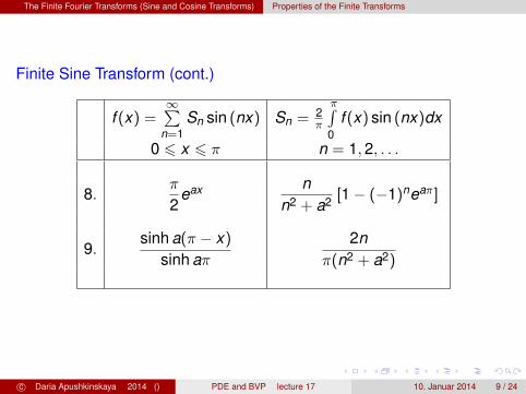
Finite Sine Transform (cont.)

f (x) =∞∑


π

π∫0

f (x) sin (nx)dx

0 6 x 6 π n = 1,2, . . .

8.π

2eax n

n2 + a2 [1− (−1)neaπ]

9.sinh a(π − x)

sinh aπ2n

π(n2 + a2)



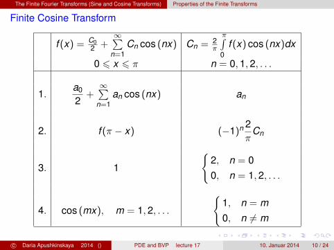
Finite Cosine Transform

f (x) = C02 +

∞∑n=1

Cn cos (nx) Cn = 2π

π∫0

f (x) cos (nx)dx

0 6 x 6 π n = 0,1,2, . . .

1.a0

2+

∞∑n=1

an cos (nx) an

2. f (π − x) (−1)n 2π

Cn

3. 1

{2, n = 00, n = 1,2, . . .

4. cos (mx), m = 1,2, . . .

{1, n = m0, n 6= m



Finite Cosine Transform (cont.)

f (x) = C02 +

∞∑n=1


π∫0

f (x) cos (nx)dx

0 6 x 6 π n = 0,1,2, . . .

5. x

π, n = 02πn2 [(−1)n − 1] , n = 1,2, . . .

6. x2

2π2/3, n = 04n2 (−1)n, n = 1,2, . . .

7. − log(2 sin (x/2))

0, n = 01n, n = 1,2, . . .



Finite Cosine Transform

f (x) = C02 +

∞∑n=1


π∫0

f (x) cos (nx)dx

0 6 x 6 π n = 0,1,2, . . .

8.1a

eax 2π

[(−1)neaπ − 1

n2 + a2

]

9.

{1, 0 < x < a−1, a < x < π

2π

(2a− π), n = 0

4nπ

sin (na), n = 1,2, . . .


The Finite Fourier Transforms (Sine and Cosine Transforms) Solving Problems via Finite Transforms

Solving a Nonhomogeneous BVP via the Finite Sine Transform

Consider the nonhomogeneous wave equation

Problem 17-1To find the function u(x , t) that satisfies

PDE: utt = uxx + sin (πx), 0 < x < 1, 0 < t <∞

BCs:

{u(0, t) = 0u(1, t) = 0

0 < t <∞

ICs:

{u(x ,0) = 1ut (x ,0) = 0

0 6 x 6 1



Step 1. (Determine the transform)Since the x-variable ranges from 0 to 1, we use a finite transform.

We could solve this problem with the Laplace transform bytransforming t (it would involve about the same level of difficulty asthe finite sine transform).



Step 2. (Carry out the transformation)Transforming the PDE and ICs we get the new IVP forSn(t) = S[u]

Problem 17-1a

ODE:d2Sn

dt2 + (nπ)2Sn =

{1, n = 10, n = 2,3, . . .

,

ICs:

Sn(0) =

{4/(nπ), n = 1,3, . . .

0, n = 2,4, . . .dSn(0)

dt= 0, n = 1,2, . . .



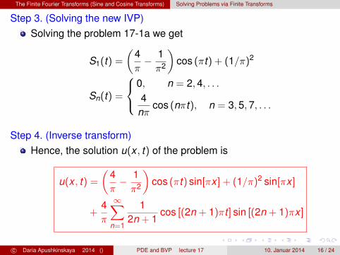
Step 3. (Solving the new IVP)Solving the problem 17-1a we get

S1(t) =

(4π− 1π2

)cos (πt) + (1/π)2

Sn(t) =

0, n = 2,4, . . .4

nπcos (nπt), n = 3,5,7, . . .

Step 4. (Inverse transform)Hence, the solution u(x , t) of the problem is

u(x , t) =

(4π− 1π2

)cos (πt) sin[πx ] + (1/π)2 sin[πx ]

+4π

∞∑n=1

12n + 1

cos [(2n + 1)πt ] sin [(2n + 1)πx ]



RemarksIn order to apply the finite sine or cosine transform, the BCs atx = 0 and x = L must both be of the form

u(0, t) = f (t)u(L, t) = g(t)

}(use sine transform)

ux (0, t) = f (t)ux (L, t) = g(t)

}(use cosine transform)

In other words, the BCs

u(0, t) = f (t) and ux (L, t) = g(t)

wouldn’t work. Also BCs like ux (0, t) + hu(0, t) = 0 don’t apply.



Remarks (cont.)In order to apply the finite sine and cosine transforms, theequation shouldn’t contain first-order derivatives in x (since thesine transform of the first derivative involves the cosine transformand vice versa).

The finite sine- and cosine-transform method essentially resolvesall functions in the original problem (like utt , uxx , the ICs, BCs) intoa Fourier sine and cosine series, solves a sequence of problems(ODE) for the Fourier coefficients, and then adds up the result.


The Vibrating Drumhead (Wave Equation in Polar Coordinates)



€

un (x, t) = sin(nπx /L) an sin(nπct /L) + bn cos(nπct /L)[ ]n =1,2,3,...




We want to find the vibrations of a circular drumhead with givenboundary and initial conditions.

Problem 17-2To find the function u(r , θ, t) that satisfies

PDE: utt = c2 (urr + 1r ur + 1

r2 uθθ

), 0 < r < 1

BC: u(1, θ, t) = 0, 0 < θ,2π, 0 < t <∞

ICs:

{u(r , θ, 0) = f (r , θ)

ut (r , θ, 0) = g(r , θ)



Recall that for violin-string problem the solution is a superpositionof an infinite number of simple vibrations.

If we approach the drumhead in a similar manner, we will look forsolutions of the form

u(r , θ, t) = U(r , θ)T (t). (17.1)

This gives the shape U(r , θ) of the vibrations times the oscillatoryfactor T (t).



Step 1. (Separation of Variables)

Substituting (17.1) into PDE and BC, we arrive at the equationsUrr +

1r

Ur +1r2 Uθθ + λ2U = 0 (Helmholtz equation)

U(1, θ) = 0

T ′′ + λ2c2T = 0 (Simple harmonic motion)

We now have to find the shapes U(r , θ) of the fundamentalvibrations Urr +

1r

Ur +1r2 Uθθ + λ2U = 0

U(1, θ) = 0(17.2)



Step 1. (Separation of Variables)

(17.2) is the Helmholtz eigenvalue problem (very famous), and ourpurpose is to seek all λ’s (if any) that yield nonzero solutions.

Step 2. (Solving of the Helmholtz Eigenvalue Problem)

To solve (17.2) we let U(r , θ) = R(r)Θ(θ) and plug it into (17.2).Doing this, we arrive at

r2R′′ + rR′ + (λ2r2 − n2)R = 0R(1) = 0R(0) <∞ (Physical condition)

Θ′′ + n2Θ = 0

Note that we have chosen the new separation constant n2,n = 0,1,2, . . . .


Date post:	28-Apr-2018
Category:	Documents
Upload:	lamnguyet
View:	219 times
Download:	1 times

PDE and Boundary-Value Problems Winter Term …€¦ · · 2014-01-10PDE and Boundary-Value...

Documents