PDE Control Methods: Stabilization Methods for KdV equation Eduardo Cerpa Universidad T´ ecnica Federico Santa Mar´ ıa, Chile GIPSA-lab, Grenoble January 2017 E. Cerpa (UTFSM) PDE Control Methods 1 / 103
Transcript
PDE Control Methods:Stabilization Methods for KdV equation
3 Boundary Control from the rightFinite Dimensional CaseInfinite Dimensional CaseApplication to our ProblemNumerical Simulations
4 Boundary Control from the leftControl DesignLinear SystemNonlinear SystemOutput feedback
E. Cerpa (UTFSM) PDE Control Methods 2 / 103
Control System
E. Cerpa (UTFSM) PDE Control Methods 3 / 103
Korteweg-de Vries equation 1895
Function u = u(t, x) models for a time t the amplitude of the water wave atposition x. The nonlinear dispersive partial differential equation, namedKorteweg-de Vries equation and abbreviated as KdV, describes approximatelylong waves in water of relatively shallow depth
ut + uxxx + uux = 0, x ∈ R, t ∈ R
E. Cerpa (UTFSM) PDE Control Methods 4 / 103
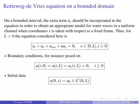
Korteweg-de Vries equation on a bounded domain
On a bounded interval, the extra term ux should be incorporated in theequation in order to obtain an appropriate model for water waves in a uniformchannel when coordinates x is taken with respect to a fixed frame. Thus, forL > 0 the equation considered here is
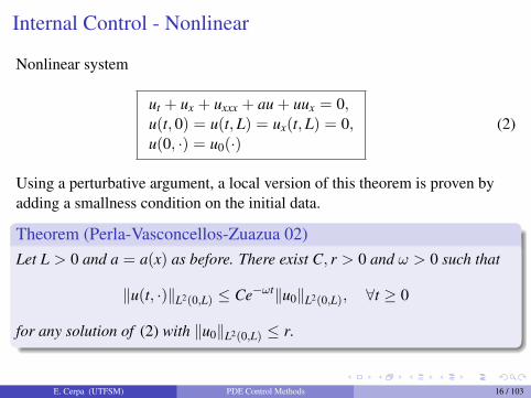
ut + ux + uxxx + uux = 0, x ∈ [0,L], t ≥ 0
+ Boundary conditions, for instance posed on
u(t, 0) = u(t,L) = ux(t,L) = 0, t ≥ 0
+ Initial datau(0, x) = u0 ∈ L2(0,L)
E. Cerpa (UTFSM) PDE Control Methods 5 / 103
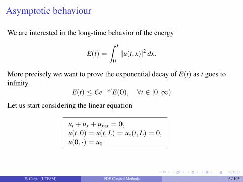
Asymptotic behaviour
We are interested in the long-time behavior of the energy
E(t) =
∫ L
0|u(t, x)|2 dx.
More precisely we want to prove the exponential decay of E(t) as t goes toinfinity.
Theorem (Pazoto 05)Let L > 0, a = a(x) as before and R > 0. There exist C = C(R) > 0 andω = ω(R) > 0 such that
‖u(t, ·)‖L2(0,L) ≤ Ce−ωt‖u0‖L2(0,L), ∀t ≥ 0
for any solution of (3) with ‖u0‖L2(0,L) ≤ R.
This result was proved in [P-V-Z 02] by assuming
∃δ > 0, (0, δ) ∪ (L− δ, L) ⊂ O
which has been removed by Pazoto.E. Cerpa (UTFSM) PDE Control Methods 17 / 103
Linear System on a noncritical caseNo damping (a(x) = 0) and L /∈ N .We have the observability inequality for T = 1
∀u0 ∈ L2(0,L), C‖ux(·, 0)‖L2(0,T) ≥ ‖u0‖L2(0,L)
Integrating with respect to time
ddt
∫ L
0|u(t, x)|2 dx = −|ux(t, 0)|2
from t = 0 to t = 1 we get∫ L
0|u(1, x)|2 dx−
∫ L
0|u0(x)|2 dx
= −∫ 1
0|ux(s, 0)|2 ds ≤ − 1
C2
∫ L
0|u0(x)|2 dx,
that implies ∫ L
0|u(1, x)|2 dx ≤ C2 − 1
C2
∫ L
0|u0(x)|2 dx.
E. Cerpa (UTFSM) PDE Control Methods 18 / 103
Linear System on a noncritical case
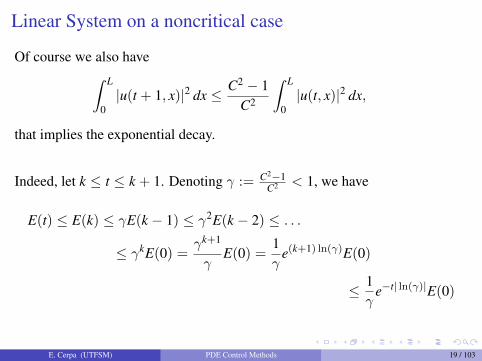
Of course we also have∫ L
0|u(t + 1, x)|2 dx ≤ C2 − 1
C2
∫ L
0|u(t, x)|2 dx,
that implies the exponential decay.
Indeed, let k ≤ t ≤ k + 1. Denoting γ := C2−1C2 < 1, we have
E(t) ≤ E(k) ≤ γE(k − 1) ≤ γ2E(k − 2) ≤ . . .
≤ γkE(0) =γk+1
γE(0) =
1γ
e(k+1) ln(γ)E(0)
≤ 1γ
e−t| ln(γ)|E(0)
E. Cerpa (UTFSM) PDE Control Methods 19 / 103
Linear System on a critical caseWith damping a(x)u active in O and L ∈ N . From∫ L
0(ut + ux + uxxx + au)u dx = 0
we get
dds
∫ L
0|u(s, x)|2 dx = −|ux(s, 0)|2 −
∫ L
0a(x)|u(s, x)|2 dx ≤ 0
and then by integrating on (0, 1) we obtain∫ L
0|u(1, x)|2 dx−
∫ L
0|u0(x)|2 dx
= −∫ 1
0|ux(s, 0)|2 ds−
∫ 1
0
∫ L
0a(x)|u(s, x)|2 dxds.
E. Cerpa (UTFSM) PDE Control Methods 20 / 103
Linear System on a critical case
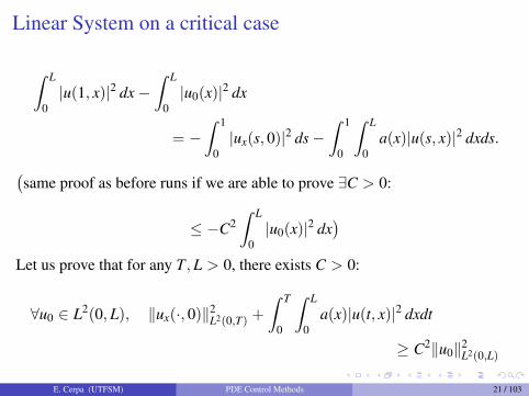
∫ L
0|u(1, x)|2 dx−
∫ L
0|u0(x)|2 dx
= −∫ 1
0|ux(s, 0)|2 ds−
∫ 1
0
∫ L
0a(x)|u(s, x)|2 dxds.
(same proof as before runs if we are able to prove ∃C > 0:
≤ −C2∫ L
0|u0(x)|2 dx
)Let us prove that for any T,L > 0, there exists C > 0:
∀u0 ∈ L2(0,L), ‖ux(·, 0)‖2L2(0,T) +
∫ T
0
∫ L
0a(x)|u(t, x)|2 dxdt
≥ C2‖u0‖2L2(0,L)
E. Cerpa (UTFSM) PDE Control Methods 21 / 103
Linear System on a critical caseBy integrating by parts∫ L
0(ut + ux + uxxx + au)(T − t)u dx = 0
we obtain
‖u0‖2L2(0,L) ≤
1T‖u‖2
L2(0,T;L2(0,L))
+ ‖ux(·, 0)‖2L2(0,T) + 2
∫ T
0
∫ L
0a(x)|u(t, x)|2 dxdt
and therefore we will be done if we prove that there exists a constant K > 0such that
K‖u‖2L2(0,T;L2(0,L)) ≤ ‖ux(·, 0)‖2
L2(0,T)
+
∫ T
0
∫ L
0a(x)|u(t, x)|2 dxdt
E. Cerpa (UTFSM) PDE Control Methods 22 / 103
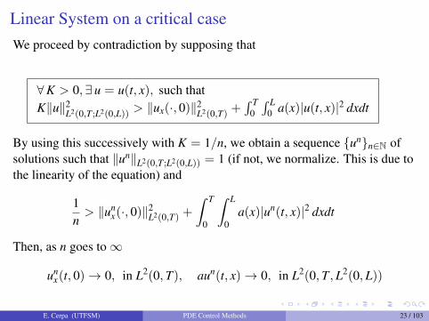
Linear System on a critical caseWe proceed by contradiction by supposing that
∀K > 0, ∃ u = u(t, x), such thatK‖u‖2
L2(0,T;L2(0,L)) > ‖ux(·, 0)‖2L2(0,T) +
∫ T0
∫ L0 a(x)|u(t, x)|2 dxdt
By using this successively with K = 1/n, we obtain a sequence {un}n∈N ofsolutions such that ‖un‖L2(0,T;L2(0,L)) = 1 (if not, we normalize. This is due tothe linearity of the equation) and
1n> ‖un
x(·, 0)‖2L2(0,T) +
∫ T
0
∫ L
0a(x)|un(t, x)|2 dxdt
Then, as n goes to∞
unx(t, 0)→ 0, in L2(0,T), aun(t, x)→ 0, in L2(0,T,L2(0,L))
E. Cerpa (UTFSM) PDE Control Methods 23 / 103
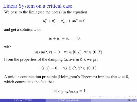
Linear System on a critical caseWe pass to the limit (see the notes) in the equation
unt + un
x + unxxx + aun = 0.
and get a solution u of
ut + ux + uxxx = 0.
witha(x)u(t, x) = 0 ∀x ∈ [0,L], ∀t ∈ (0,T)
From the properties of the damping (active in O), we get
u(t, x) = 0, ∀x ∈ O, ∀t ∈ (0,T).
A unique continuation principle (Holmgrem’s Theorem) implies that u = 0,which contradicts the fact that
‖u‖L2(0,T;L2(0,L)) = 1
E. Cerpa (UTFSM) PDE Control Methods 24 / 103
Stabilization of the Linear System
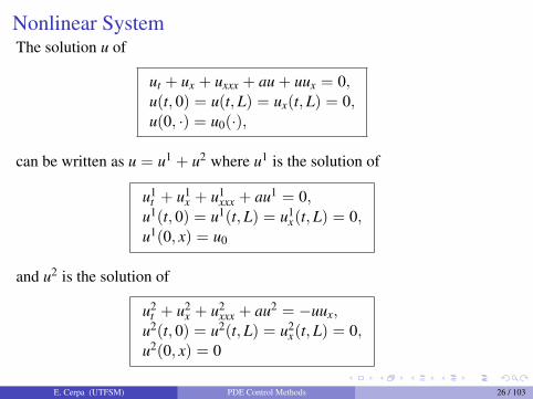
ut + ux + uxxx + au = 0,u(t, 0) = u(t,L) = ux(t,L) = 0,u(0, ·) = u0(·),
Theorem (Perla-Vasconcellos-Zuazua 02)Let L > 0 and a = a(x) as before. There exist C, ω > 0:
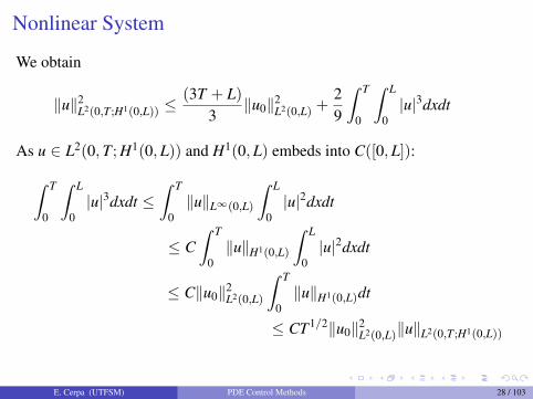
As u ∈ L2(0,T; H1(0,L)) and H1(0,L) embeds into C([0,L]):∫ T
0
∫ L
0|u|3dxdt ≤
∫ T
0‖u‖L∞(0,L)
∫ L
0|u|2dxdt
≤ C∫ T
0‖u‖H1(0,L)
∫ L
0|u|2dxdt
≤ C‖u0‖2L2(0,L)
∫ T
0‖u‖H1(0,L)dt
≤ CT1/2‖u0‖2L2(0,L)‖u‖L2(0,T;H1(0,L))
E. Cerpa (UTFSM) PDE Control Methods 28 / 103
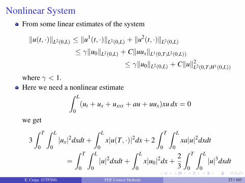
Nonlinear System
We obtain
‖u‖2L2(0,T;H1(0,L)) ≤
(8T + 2L)
3‖u0‖2
L2(0,L) +TC27‖u0‖4
L2(0,L)
which gives the existence of C > 0 such that
‖u(t, ·)‖L2(0,L) ≤ ‖u0‖L2(0,L)
{γ + C‖u0‖L2(0,L) + C‖u0‖3
L2(0,L)
}Given ε > 0 small enough such that (γ + ε) < 1, we can take r small enoughso that r + r3 < ε
C , in order to have
‖u(t, ·)‖L2(0,L) ≤ (γ + ε)‖u0‖L2(0,L)
The rest of the proof runs as before thanks to the fact that (γ + ε) < 1.
E. Cerpa (UTFSM) PDE Control Methods 29 / 103
Stabilization of the Nonlinear System
We have introduced an internal damping mechanism in order to be sure theenergy of the system decreases to zero in an exponential way. We have proveda local result for the KdV equation.
Theorem (Perla-Vasconcellos-Zuazua 02)Let L > 0 and a = a(x) as before. There exist C, r, ω > 0:
‖u(t, ·)‖L2(0,L) ≤ Ce−ωt‖u0‖L2(0,L), ∀t ≥ 0
for any solution of KdV with ‖u0‖L2(0,L) ≤ r.
E. Cerpa (UTFSM) PDE Control Methods 30 / 103
Remark
Similar results have been proven recently for coupled systems of KdVequations. See [Capistrano-Fihlo, Komornik, and Pazoto. 2014],[Pazoto, Souza, 2014 and 2013], Massarolo, Perla-Mezala, and Pazoto,2011], [Nina, Pazoto, and Rosier, 2011], [Pazoto, Rosier, 2010].
That could seem strange, but as mentioned before, a similar phenomenaappears when studying the controllability of the system from the rightNeumann boundary condition. The linear system is controllable if andonly if L is not critical but in despite of that the nonlinear system isalways controllable.
E. Cerpa (UTFSM) PDE Control Methods 31 / 103
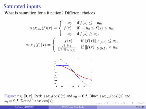
Saturated inputsWhat is saturation for a function? Different choices
satloc(f )(x) =
−u0 if f (x) ≤ −u0,f (x) if − u0 ≤ f (x) ≤ u0,
u0 if f (x) ≥ u0,
sat2(f )(x) =
{f (x) if ‖f (x)‖L2(0,L) ≤ u0,
f (x)u0‖f (x)‖L2(0,L)
if ‖f (x)‖L2(0,L) ≥ u0.
Figure: x ∈ [0, π]. Red: sat2(cos)(x) and u0 = 0.5, Blue: satloc(cos)(x) andu0 = 0.5, Dotted lines: cos(x).
E. Cerpa (UTFSM) PDE Control Methods 32 / 103
Saturated inputs
Let us consider the KdV equation controlled by a saturated distributed controlas follows
where sat is any of previous saturations, and a is a localized function as inprevious sections.
Theorem (Marx, EC, Prieur, Andrieu, under review)There exist a positive value µ? and a class K function α0 : R≥0 → R≥0 suchthat for any y0 ∈ L2(0,L), the mild solution y of saturated-KdV satisfies
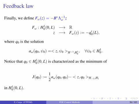
is globally well posed in H10(0,L). Moreover, the solutions decay to zero with
an exponential rate of 2ω, i.e.,
∃C > 0, ∀u0 ∈ H10(0,L), ‖u(t, ·)‖H1
0≤ Ce−2ωt‖u0‖H1
0.
E. Cerpa (UTFSM) PDE Control Methods 38 / 103
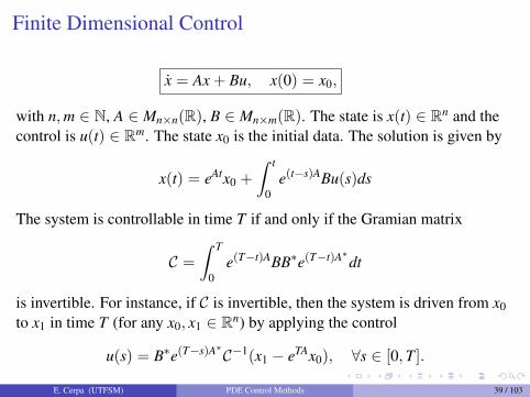
Finite Dimensional Control
x = Ax + Bu, x(0) = x0,
with n,m ∈ N, A ∈ Mn×n(R), B ∈ Mn×m(R). The state is x(t) ∈ Rn and thecontrol is u(t) ∈ Rm. The state x0 is the initial data. The solution is given by
x(t) = eAtx0 +
∫ t
0e(t−s)ABu(s)ds
The system is controllable in time T if and only if the Gramian matrix
C =
∫ T
0e(T−t)ABB∗e(T−t)A∗dt
is invertible. For instance, if C is invertible, then the system is driven from x0to x1 in time T (for any x0, x1 ∈ Rn) by applying the control
u(s) = B∗e(T−s)A∗C−1(x1 − eTAx0), ∀s ∈ [0,T].
E. Cerpa (UTFSM) PDE Control Methods 39 / 103
Gramian-based stabilizationLet us see how the Gramian matrix can also be used to stabilize the system.Let us suppose the system is controlable. Thus,
CT = e−TACe−TA∗ =
∫ T
0e−tABB∗e−tA∗dt
is invertible and we can define the feedback control
u(t) = −B∗C−1T x(t).
By applying a Lyapunov method, it can be easily proven the following (seethe notes).
Theorem∃M, µ > 0 such that solutions of x(t) = (A− BB∗C−1
T )x(t), satisfies
|x(t)| ≤ Me−µt|x(0)|, ∀t ≥ 0.
E. Cerpa (UTFSM) PDE Control Methods 40 / 103
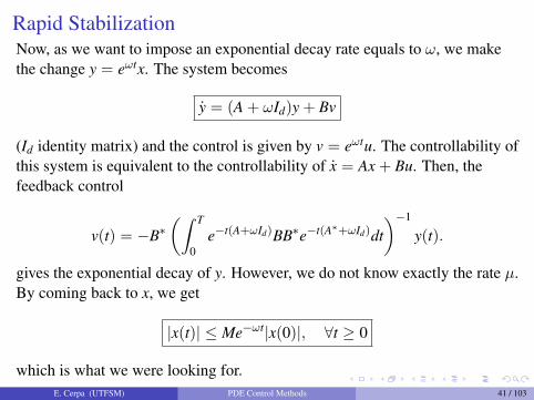
Rapid StabilizationNow, as we want to impose an exponential decay rate equals to ω, we makethe change y = eωtx. The system becomes
y = (A + ωId)y + Bv
(Id identity matrix) and the control is given by v = eωtu. The controllability ofthis system is equivalent to the controllability of x = Ax + Bu. Then, thefeedback control
v(t) = −B∗(∫ T
0e−t(A+ωId)BB∗e−t(A∗+ωId)dt
)−1
y(t).
gives the exponential decay of y. However, we do not know exactly the rate µ.By coming back to x, we get
|x(t)| ≤ Me−ωt|x(0)|, ∀t ≥ 0
which is what we were looking for.E. Cerpa (UTFSM) PDE Control Methods 41 / 103
Rapid stabilizationAn improvement of this method: let us consider the matrix
Cω,∞ =
∫ ∞0
e−t(A+ωId)BB∗e−t(A∗+ωId)dt
We obtain(A + ωId)Cω,∞ + Cω,∞(A + ωId)∗ = BB∗
and then if we use the control
u(t) = −B∗C−1ω,∞x(t)
in x = Ax + Bu, then we obtain
(A− BB∗C−1ω,∞) = Cω,∞(−A∗ − 2ωId)C−1
ω,∞
In particular, if A∗ = −A, then the eigenvalues of systemx = (A− BB∗C−1
ω,∞)x are exactly the eigenvalues of A shifted 2ω units to theleft in the complex plane:
|x(t)| ≤ Me−2ωt|x(0)|, ∀t ≥ 0.
E. Cerpa (UTFSM) PDE Control Methods 42 / 103
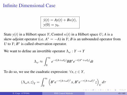
Infinite Dimensional Case
y(t) = Ay(t) + Bκ(t),y(0) = y0.
State y(t) in a Hilbert space Y; Control κ(t) in a Hilbert space U; A is askew-adjoint operator (i.e. A∗ = −A) in Y; B is an unbounded operator fromU to Y; B∗ is called observation operator.
We want to define an invertible operator Λω : Y → Y
Λω ≈∫ ∞
0e−t(A+ωId)BB∗e−t(A∗+ωId)dt
To do so, we use the cuadratic expression: ∀x, z ∈ Y,
(Λωx, z)Y =
∫ ∞0
(B∗e−τ(A+ωI)∗x,B∗e−τ(A+ωI)∗z
)U
dτ
E. Cerpa (UTFSM) PDE Control Methods 43 / 103
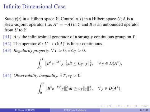
Infinite Dimensional Case
State y(t) in a Hilbert space Y; Control κ(t) in a Hilbert space U; A is askew-adjoint operator (i.e. A∗ = −A) in Y and B is an unbounded operatorfrom U to Y .
(H1) A is the infinitesimal generator of a strongly continuous group on Y .
(H2) The operator B : U → D(A)′ is linear continuous.
(H3) Regularity property. ∀T > 0, ∃CT > 0:∫ T
0‖B∗e−tA∗y‖2
Udt ≤ CT‖y‖2Y , ∀ y ∈ D(A∗).
(H4) Observability inequality. ∃T, cT > 0:∫ T
0‖B∗e−tA∗y‖2
Udt ≥ cT‖y‖2Y , ∀ y ∈ D(A∗).
E. Cerpa (UTFSM) PDE Control Methods 44 / 103
Infinite Dimensional Case
Theorem (Urquiza 05)Consider A and B such that (H1)-(H4) hold. For any ω > 0:
(i) The symmetric positive operator Λω defined above is coercive and anisomorphism on Y.
(ii) Let Fω := −B∗Λ−1ω . The operator A + BFω is the infinitesimal generator
of a strongly continuous semigroup on Y.
(iii) The closed-loop system with feedback law Fω(y(t)) is exponentiallystable with a decay rate 2ω:
∃C > 0, ∀y0 ∈ Y, ‖et(A+BFω)y0‖Y ≤ Ce−2ωt‖y0‖Y .
E. Cerpa (UTFSM) PDE Control Methods 45 / 103
Application to our Problem
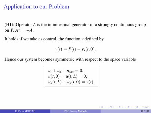
(H1): Operator A is the infinitesimal generator of a strongly continuous groupon Y , A∗ = −A.
It holds if we take as control, the function v defined by
v(t) = F(t)− yx(t, 0).
Hence our system becomes symmetric with respect to the space variable
We can rewrite latter system in the abstract form by defining U := L2(0,T),Y := L2(0,L) and
D(A) :={
w ∈ H3(0,L); w(0) = w(L) = 0,w′(0) = w′(L)},
Aw := −w′ − w′′′,
B : s ∈ R 7−→ Ls ∈ D(A∗)′,
Ls : z ∈ D(A∗) 7−→ szx(L) ∈ R.
It is not difficult to see that A∗ = −A and that
(Aw,w)L2(0,L) = 0, ∀w ∈ D(A).
Hence, from classical semigroup results, one sees that the operator A satisfies(H1). We also see that (H2) holds for the operator B.
E. Cerpa (UTFSM) PDE Control Methods 47 / 103
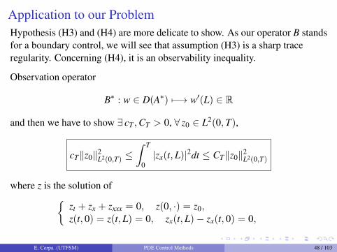
Application to our ProblemHypothesis (H3) and (H4) are more delicate to show. As our operator B standsfor a boundary control, we will see that assumption (H3) is a sharp traceregularity. Concerning (H4), it is an observability inequality.
Observation operator
B∗ : w ∈ D(A∗) 7−→ w′(L) ∈ R
and then we have to show ∃ cT ,CT > 0, ∀ z0 ∈ L2(0,T),
cT‖z0‖2L2(0,T) ≤
∫ T
0|zx(t,L)|2dt ≤ CT‖z0‖2
L2(0,T)
where z is the solution of{zt + zx + zxxx = 0, z(0, ·) = z0,z(t, 0) = z(t,L) = 0, zx(t,L)− zx(t, 0) = 0,
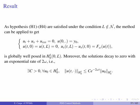
is globally well posed in H10(0,L). Moreover, the solutions decay to zero with
an exponential rate of 2ω, i.e.,
∃C > 0, ∀u0 ∈ H10 , ‖u(t, ·)‖H1
0≤ Ce−2ωt‖u0‖H1
0.
E. Cerpa (UTFSM) PDE Control Methods 57 / 103
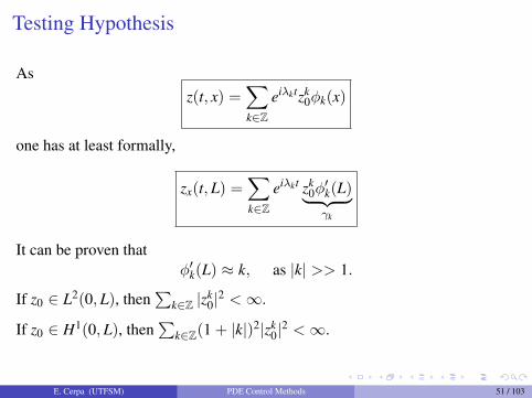
Numerical Simulations
Evolution of the solution when ω = 2 (left) and ω = 3 (right).
E. Cerpa (UTFSM) PDE Control Methods 58 / 103
Numerical Simulations
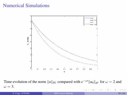
Time-evolution of the norm ‖u‖H1 compared with e−ωt‖u0‖H1 for ω = 2 andω = 3.
E. Cerpa (UTFSM) PDE Control Methods 59 / 103
Remarks
By using a finite-dimensional method based on the Gramian matrix wehave design some feedback controls which make the linear KdVequation stable with an exponential decay rate as large as desired.
This method can not be applied if the underlying spatial operator is notskew-adjoint.
For that reason, we consider a first order boundary condition on(ux(t,L)− ux(t, 0) instead of ux(t,L).
E. Cerpa (UTFSM) PDE Control Methods 60 / 103
Remarks
A major difficulty in order to consider the nonlinear KdV equation is to dealwith the technical point of well-posedness of the equation with the convenientboundary conditions. Is the system
With this boundary conditions there is no Kato smoothing effect allowing usto deal with the nonlinearity uux in the well-posedness framework.
E. Cerpa (UTFSM) PDE Control Methods 61 / 103
Remarks
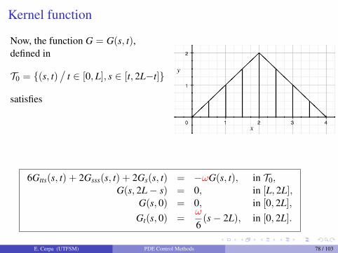
In [Coron and Lu, 2014] the authors apply a new design strategy (similar toBackstepping method) in order to define a control law acting on the right-handside of the interval. They do not need to work with a skew-adjoint operatorand therefore they obtain stabilization results for the nonlinear KdV equation
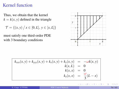
6Gtts(s, t) + 2Gsss(s, t) + 2Gs(s, t) = −ωG(s, t), in T0,G(s, 2L− s) = 0, in [L, 2L],
G(s, 0) = 0, in [0, 2L],
Gt(s, 0) =ω
6(s− 2L), in [0, 2L].
E. Cerpa (UTFSM) PDE Control Methods 78 / 103
Kernel function
Let us transform this system into an integral one.
We write the equation in variables (η, ξ), integrate ξ in (0, τ) and usethat 6Gts(η, 0) = ω.
We integrate τ in (0, t) and use that Gs(η, 0) = 0.
We integrate η in (s, 2L− t) and use that G(2L− t, t) = 0.
Thus, we can write the following integral form for G = G(s, t)
G(s, t) = −ωt6
(2L− t − s)
+16
∫ 2L−t
s
∫ t
0
∫ τ
0
(2Gsss(η, ξ) + 2Gs(η, ξ) + ωG(η, ξ)
)dξdτdη.
E. Cerpa (UTFSM) PDE Control Methods 79 / 103
Kernel functionTo prove that such a function G = G(s, t) exists, we use the method ofsuccessive approximations. We take as an initial guess
G1(s, t) = −ωt6
(2L− t − s)
and define the recursive formula as follows,
Gn+1(s, t) =16
∫ 2L−t
s
∫ t
0
∫ τ
0
(2Gn
sss(η, ξ)
+ 2Gns (η, ξ) + ωGn(η, ξ)
)dξdτdη.
Performing some computations, we get for instance
G2(s, t) =1
108
{t3(ω − ω2L +
ω2t4)(
2L− t − s)
+t3ω2
4[(2L− t)2 − s2]},
E. Cerpa (UTFSM) PDE Control Methods 80 / 103
Kernel function
... and more generally the following formula
Gk(s, t) =
k∑i=1
(ai
kt2k−1 + bikt2k)[(2L− t)i − si],
where the coefficients satisfy bkk = 0 and more importantly, there exist
positive constants M,B such that, for any k ≥ 1 and any (s, t) ∈ T0
∣∣Gk(s, t)∣∣ ≤ M
Bk
(2k)!(t2k−1 + t2k).
This implies that the series∑∞
n=1 Gn(s, t) is uniformly convergent in T0.
E. Cerpa (UTFSM) PDE Control Methods 81 / 103
Kernel functionWe get a solution of our integral equation. Indeed,
G = G1 +
∞∑n=1
Gn+1
= G1 +16
∞∑n=1
∫ 2L−t
s
∫ t
0
∫ τ
0
(2Gn
sss(η, ξ)
+ 2Gns (η, ξ) + ωGn(η, ξ)
)dξdτdη
= G1 +16
∫ 2L−t
s
∫ t
0
∫ τ
0
(2∞∑
n=1
Gnsss(η, ξ)
+ 2∞∑
n=1
Gns (η, ξ) + ω
∞∑n=1
Gn(η, ξ))
dξdτdη
= G1 +16
∫ 2L−t
s
∫ t
0
∫ τ
0
(2Gsss(η, ξ) + 2Gs(η, ξ) + ωG(η, ξ)
)dξdτdη.
E. Cerpa (UTFSM) PDE Control Methods 82 / 103
Kernel function
We plot the gain kernel k(0, y) as a function of y ∈ [0,L] for the length (a)L = 1 (non-critical). ω = 1.
0.0 0.2 0.4 0.6 0.8 1.0-0.08
-0.06
-0.04
-0.02
0.00
HaL
E. Cerpa (UTFSM) PDE Control Methods 83 / 103
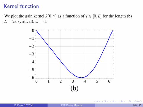
Kernel function
We plot the gain kernel k(0, y) as a function of y ∈ [0,L] for the length (b)L = 2π (critical). ω = 1.
0 1 2 3 4 5 6-6
-5
-4
-3
-2
-1
0
HbL
E. Cerpa (UTFSM) PDE Control Methods 84 / 103
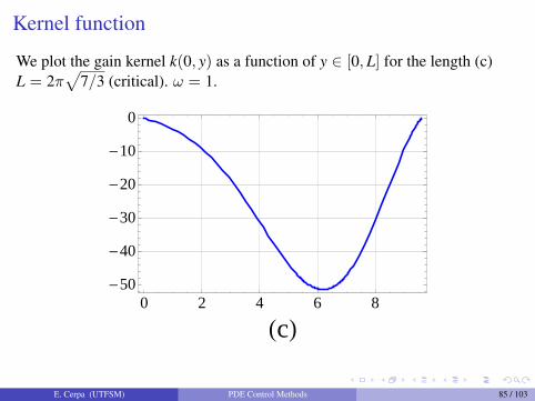
Kernel function
We plot the gain kernel k(0, y) as a function of y ∈ [0,L] for the length (c)L = 2π
√7/3 (critical). ω = 1.
0 2 4 6 8-50
-40
-30
-20
-10
0
HcL
E. Cerpa (UTFSM) PDE Control Methods 85 / 103
Stability Linear SystemWe know that the target system is exponentially stable. In order to get thesame conclusion for the original linear system the method we are applyinguses the inverse transformation Π−1. For that, we introduce a kernel function`(x, y) which satisfies
The existence and uniqueness of such a kernel ` = `(x, y) are proven in thesame way than for the kernel k = k(x, y) previously. Once we have defined` = `(x, y), it is easy to see that the transformation Π−1 is characterized by
u(x) = Π−1(v(x)) := v(x) +
∫ L
x`(x, y)v(y)dy.
E. Cerpa (UTFSM) PDE Control Methods 86 / 103
Stability Linear System
The operator Π : L2(0,L)→ L2(0,L), is continuous and consequently wehave the existence of a positive constant Dκ such that
‖Π(f )‖L2(0,L) ≤ Dκ‖f‖L2(0,L), ∀f ∈ L2(0,L).
The map Π−1 : L2(0,L)→ L2(0,L) is also continuous and therefore we getthe existence of a positive constant D` such that
‖Π−1(f )‖L2(0,L) ≤ D`‖f‖L2(0,L), ∀f ∈ L2(0,L).
E. Cerpa (UTFSM) PDE Control Methods 87 / 103
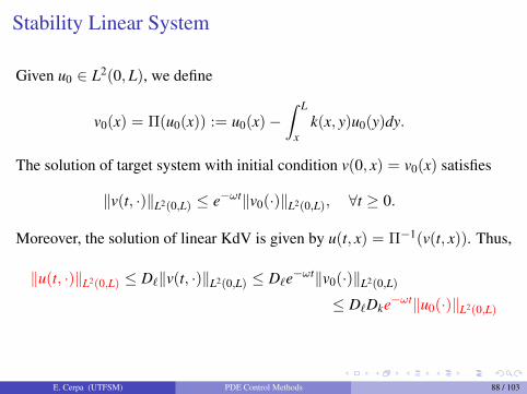
Stability Linear System
Given u0 ∈ L2(0,L), we define
v0(x) = Π(u0(x)) := u0(x)−∫ L
xk(x, y)u0(y)dy.
The solution of target system with initial condition v(0, x) = v0(x) satisfies
‖v(t, ·)‖L2(0,L) ≤ e−ωt‖v0(·)‖L2(0,L), ∀t ≥ 0.
Moreover, the solution of linear KdV is given by u(t, x) = Π−1(v(t, x)). Thus,
Let u = u(t, x) be a solution of the nonlinear KdV equation with the controlgiven by
K(t) =
∫ L
0k(0, y)u(t, y)dy,
Then, v = Π(u(t, x)) satisfies
vt(t, x) + vx(t, x) + vxxx(t, x) + ωv(t, x) =
−(
v(t, x) +
∫ L
x`(x, y)v(t, y)dy
)(vx(t, x) +
∫ L
x`x(x, y)v(t, y)dy
)with homogeneous boundary conditions
v(t, 0) = 0, v(t,L) = 0, vx(t,L) = 0.
E. Cerpa (UTFSM) PDE Control Methods 89 / 103
Nonlinear System
We multiply by v and integrate in (0,L) to obtain
ddt
∫ L
0|v(t, x)|2dx = −|vx(t, 0)|2
− 2ω∫ L
0|v(t, x)|2dx− 2
∫ L
0v(t, x)F(t, x)dx
where the term F = F(t, x) is given by
F(t, x) = v(t, x)
∫ L
x`x(x, y)v(t, y)dy + vx(t, x)
∫ L
x`(x, y)v(t, y)dy
+
(∫ L
x`(x, y)v(t, y)dy
)(∫ L
x`x(x, y)v(t, y)dy
)
E. Cerpa (UTFSM) PDE Control Methods 90 / 103
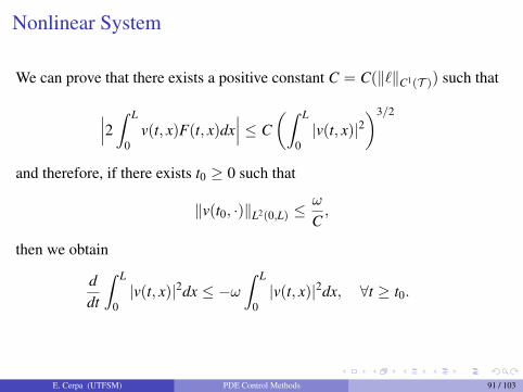
Nonlinear System
We can prove that there exists a positive constant C = C(‖`‖C1(T )) such that
∣∣∣2 ∫ L
0v(t, x)F(t, x)dx
∣∣∣ ≤ C(∫ L
0|v(t, x)|2
)3/2
and therefore, if there exists t0 ≥ 0 such that
‖v(t0, ·)‖L2(0,L) ≤ω
C,
then we obtain
ddt
∫ L
0|v(t, x)|2dx ≤ −ω
∫ L
0|v(t, x)|2dx, ∀t ≥ t0.
E. Cerpa (UTFSM) PDE Control Methods 91 / 103
Nonlinear System
Thus, we get
Theorem (EC-Coron 2013)For any ω > 0, there exist a feedback control law Kω = Kω(u(t, ·)), r > 0 andD > 0 such that
‖u(t, ·)‖L2(0,L) ≤ De−ωt‖u0‖L2(0,L), ∀t ≥ 0,
for any solution of nonlinear KdV satisfiying ‖u0‖L2(0,L) ≤ r.
E. Cerpa (UTFSM) PDE Control Methods 92 / 103
Remarks
The backstepping method has been applied to build some boundaryfeedback laws, which locally stabilize the Korteweg-de Vries equationposed on a finite interval.
Our control acts on the Dirichlet boundary condition at the left hand sideof the interval where the system evolves.
The closed-loop system is proven to be locally exponentially stable witha decay rate that can be chosen to be as large as we want.
E. Cerpa (UTFSM) PDE Control Methods 93 / 103
Remarks
Let us consider one or two control inputs at the right hand side
u(t, 0) = 0, u(t,L) = K1(t), ux(t,L) = K2(t)
To impose vt + vx + vxxx + ωv = 0, we have to vanish
As we do not have to our disposal uxx(t,L), the first term above arises thecondition k(x,L) = 0.
Moreover, to keep w(t, 0) = u(t, 0) = 0, we have to impose k(0, y) = 0 forany y ∈ (0,L). We get four boundary restrictions (the other two are onk(x, x)), the third order kernel equation satisfied by k = k(x, y) may becomeoverdetermined.
E. Cerpa (UTFSM) PDE Control Methods 94 / 103
RemarksA natural idea to deal with controls at x = L is to use
v(t, x) = u(t, x)−∫ x
0k(x, y)u(t, y)dy,
If we do so, we deal now with the extra condition ky(x, 0) = 0 for anyx ∈ (0,L). This is due to the fact that when imposing vt + vx + vxxx + ωv = 0on the target system, we get the extra term ux(t, 0)ky(x, 0) to be cancelled. Aspreviously, this fourth restriction may give an overdetermined kernel equationfor k = k(x, y).
Moreover, the existence of critical lengths when only one control isconsidered at the right end-point suggests that either the existence of thekernel or the invertibility of the corresponding map Π should fail for somespatial domains.
As mentioned before, [Coron, Liu, 2014] solve this problem changing thestructure of the transformation.
E. Cerpa (UTFSM) PDE Control Methods 95 / 103
Output feedback control
GOAL: To design a controller u = K(y(t)) depending on some partialmeasurements y(t) of the solution and not on the full state u = u(t, x).
What measurements?
The natural choice for the KdV equation should be y(t) = ux(t, 0).
Unfortunately, the system is not observable with this choice. (Critical values)
In this paper we consider the output given by
y(t) = uxx(t,L).
By using this measurement, we build an observer and apply the backsteppingmethod to design an output feedback control which exponentially stabilizesthe closed-loop system.
E. Cerpa (UTFSM) PDE Control Methods 96 / 103
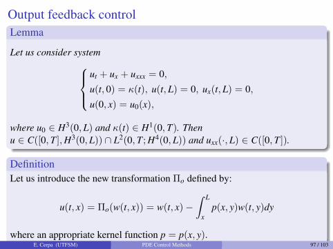
Output feedback controlLemma
Let us consider systemut + ux + uxxx = 0,
u(t, 0) = κ(t), u(t,L) = 0, ux(t,L) = 0,
u(0, x) = u0(x),
where u0 ∈ H3(0,L) and κ(t) ∈ H1(0,T). Thenu ∈ C([0,T],H3(0,L)) ∩ L2(0,T; H4(0,L)) and uxx(·,L) ∈ C([0,T]).
DefinitionLet us introduce the new transformation Πo defined by:
u(t, x) = Πo(w(t, x)) = w(t, x)−∫ L
xp(x, y)w(t, y)dy
where an appropriate kernel function p = p(x, y).E. Cerpa (UTFSM) PDE Control Methods 97 / 103
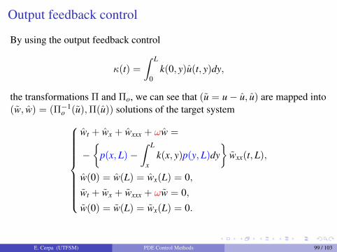
Output feedback control
By following a classical approach, we construct the following observer:ut + ux + uxxx + p(x,L)[y(t)− uxx(t,L)] = 0,
u(t, 0) = κ(t), u(t,L) = ux(t,L) = 0,
u(0, x) = 0,
(6)
y(t) = uxx(t,L).
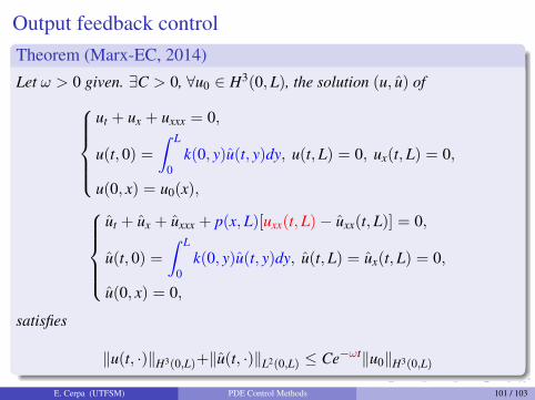
Theorem (Marx-EC, 2014)For any ω > 0, there exist a feedback law κ(t) := κ(u(t, x)), a functionp = p(x, y), and a constant C > 0 such that the coupled system (LKdV)-(6) isglobally exponentially stable with a decay rate equals to ω, i.e., for anyu0 ∈ H3(0,L) we have
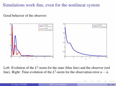
Simulations work fine, even for the nonlinear system
Good behavior of the observer:
0 2 4 6 8 100
5
10
15
t
‖u‖2L2(0,L)
‖u‖2L2(0,L)
0 2 4 6 8 100
0.5
1
1.5
2
2.5
3
3.5
t
‖u‖2L2(0,L)
Left: Evolution of the L2-norm for the state (blue line) and the observer (redline). Right: Time evolution of the L2-norm for the observation error u− u.
E. Cerpa (UTFSM) PDE Control Methods 102 / 103
Remarks
Not able to deal with the nonlinear system because regularity issues.
We are working with Swann Marx on other configurations inputs-outputsto overcome this mathematical difficulty.
Other related works by [Tang and Krstic, 2013 and 2015], [Hassan,2016].


![PDE-W-methods for parabolic problems with mixed derivativeshairer/preprints/pdew-2017.pdf · 2017-08-27 · PDE-W-methods for parabolic problems with mixed derivatives 3 [c;d], and](https://static.documents.pub/doc/80x56/5f08e3587e708231d4243542/pde-w-methods-for-parabolic-problems-with-mixed-hairerpreprintspdew-2017pdf.jpg)
