Affine invariant non-rigid shape analysis Dan Raviv Dept. of Computer Science Technion, Israel [email protected]Ron Kimmel Dept. of Computer Science Technion, Israel [email protected]Figure 1: Voronoi diagrams of ten points selected by farthest point sampling. Diffusion distances were used based on Euclidean metric (top) and an affine invariant one (bottom). Abstract Shape recognition deals with the study geometric structures. Modern surface processing methods can cope with non-rigidity - by measuring the lack of isometry, deal with similarity - by multiplying the Euclidean arc-length by the Gaussian curvature, and manage equi-affine transformations - by resorting to the special affine arc-length definition in classical affine geometry. Here, we propose a computational framework that is invariant to the affine group of transformations (similarity and equi-affine) and thus, by construction, can handle non-rigid shapes. Technically, we add the similarity invariant property to an equi-affine invariant one. Diffusion geometry encapsulates the resulting measure to robustly provide signatures and computational tools for affine invariant surface matching and comparison. 1. Introduction Differential invariants for planar shape matching and recognition were introduced to computer vision in the 80’s [49] and studied in the early 90’s [13, 12, 20, 14, 17, 11], where global invariants were com- puted in a local manner to overcome numerical sensitivity of the differential forms. Scale space entered 1 Technion - Computer Science Department - Technical Report CIS-2012-01 - 2012
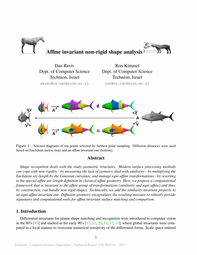
Figure 1: Voronoi diagrams of ten points selected by farthest point sampling. Diffusion distances were usedbased on Euclidean metric (top) and an affine invariant one (bottom).
Abstract
Shape recognition deals with the study geometric structures. Modern surface processing methodscan cope with non-rigidity - by measuring the lack of isometry, deal with similarity - by multiplying theEuclidean arc-length by the Gaussian curvature, and manage equi-affine transformations - by resortingto the special affine arc-length definition in classical affine geometry. Here, we propose a computationalframework that is invariant to the affine group of transformations (similarity and equi-affine) and thus,by construction, can handle non-rigid shapes. Technically, we add the similarity invariant property toan equi-affine invariant one. Diffusion geometry encapsulates the resulting measure to robustly providesignatures and computational tools for affine invariant surface matching and comparison.
1. IntroductionDifferential invariants for planar shape matching and recognition were introduced to computer vision
in the 80’s [49] and studied in the early 90’s [13, 12, 20, 14, 17, 11], where global invariants were com-puted in a local manner to overcome numerical sensitivity of the differential forms. Scale space entered
the game as a stabilizing mechanism, for example in [15], where locality was tuned by a scalar indicatinghow far one should depart from the point of interest. Along a different path, using a point matching oracleto reduce the number of derivatives, semi-differential signatures were proposed in [46, 47, 33, 39, 18].Non-local signatures, which are more sensitive to occlusions, were shown to perform favorably in holis-tic paradigms [36, 10, 35, 28]. At another end, image simplification through geometric invariant heatprocesses were introduced and experimented with during the late 90’s, [44, 2, 27]. In the beginning ofthis century, scale space theories gave birth to the celebrated scale invariant feature transform (SIFT)[30] and the affine-scale invariant feature transform ASIFT [34], that are used to successfully locaterepeatable informative (invariant) features in images.
Matching surfaces while accounting for deformations was performed with conformal mappings [29],embedding to finite dimensional Euclidean spaces [24] and infinite ones [4, 43], topological graphs [26,48], and exploiting the Gromov-Hausdorff distance [31, 7, 19]. Which are just a subset of the numerousmethods used in this exploding field. Another example, relevant to this paper is diffusion geometry,introduced in [21] for manifold learning and first applied for shape analysis in [8]. This geometry canbe constructed by the eigen-strucutre of the Laplace-Beltrami operator. The same decomposition wasrecently used in [45, 37, 38, 8] to construct surface descriptors for shape retrieval and matching.
In this paper, following the adoption of metric/differential geometry tools to image-analysis, we intro-duce a new geometry for affine invariant surface analysis. In [42, 3], an equi-affine invariant metric forsurfaces with effective Gaussian curvature were presented, while a scale invariant metric was the maintheme of [1, 9]. Here, we introduce a framework that handles both, that is, affine transformations in itsmost general form including similarity, that is scaling and isometry.
The paper is organized as follows. In Section 2 we introduce the affine invariant metric. Section 3briefly reviews the main concepts of diffusion geometry. Section 4 is dedicated to experimental results,and Section 5 concludes the paper.
2. Affine metric constructionWe model a surface (S, g) as a compact two dimensional Riemannian manifold S with a metric
tensor g. We further assume that S is embedded in R3 by a regular map S : U ⊂ R2 → R3. Theconstruction of a Euclidean metric tensor can be obtained from the re-parameterization invariant arc-length ds of a parametrized curve C(s) on S, as the simplest Euclidean invariant is length, we search forthe parameterization s that would satisfy |Cs| = 1, or explicitly,
1 = 〈Cs, Cs〉 = 〈Ss, Ss〉
=
⟨∂S
∂u
du
ds+∂S
∂v
dv
ds,∂S
∂u
du
ds+∂S
∂v
dv
ds
⟩= ds−2
(g11du
2 + 2g12dudv + g22dv2), (1)
where
gij = 〈Si, Sj〉, (2)
using the short hand notation S1 = ∂S/∂u, S2 = ∂S/∂v, and u and v are the coordinates of U . Aninfinitesimal displacement ds on the surface is thereby given by
The metric coefficients translate the surface parametrization into a Euclidean invariant distance measureon the surface.
The equi-affine transformation, defined by the linear operator AS + b, where det(A) = 1, is a bitmore tricky to deal with, see [5, 16]. Consider the curve C ∈ S parametrized by w. The equi-affinetransformation is volume preserving, and thus, its invariant metric could be constructed by restrictingthe volume defined by Su, Sv, and Cww to one. That is,
1 = det(Su, Sv, Cww) = det (Su, Sv, Sww)
= det
(Su, Sv, Suu
du2
dw2+ 2Suv
du
dw
dv
dw+ Svv
dv2
dw2+ Su
d2u
dw2+ Sv
d2v
dw2
)= dw−2 det
(Su, Sv, Suudu
2 + 2Suvdudv + Svvdv2)
= dw−2(r11du
2 + 2r12dudv + r22dv2), (4)
where now the metric elements are given by rij = det (S1, S2, Sij), and we extended the short handnotation to second order derivatives by which S11 = ∂2S
∂u2, S22 = ∂2S
∂v2, and S12 = ∂2S
∂u∂v. Note that
the second fundamental form in the Euclidean case is given by bij =√grij where g = det(gij) =
where r = det(rij) = r11r22 − r212.In [42] others and us modified the equi-affine metric to accommodate for surfaces with effective
Gaussian curvature. There, the idea was to project the metric tensor matrix qij onto the class of positivedefinite subspaces. Practically, we decompose the tensor into its eigen-structure, take the absolute valueof its eigenvalues, and compose the tensor back into a valid invariant metric.
Next, we resort to the similarity (scale and isometry) invariant metric proposed in [1], according towhich, scale invariance is obtained by multiplying the metric by the Gaussian curvature. The Gaussiancurvature is defined by the ratio between the determinants of the second and the first fundamental formsand is denoted by K. We propose to compute the Gaussian curvature of the equi-affine invariant metric,and construct a new metric by multiplying the metric elements by |K|. Specifically, consider the surface(S, q), where qij is the equi-affine invariant metric, and compute the Gaussian curvature Kq(S, q) ateach point. The affine invariant metric is defined by
hij = |Kq| qij. (6)
Let us justify the above construction of an affine invariant metric for surfaces.
2.1. Proof of invariance
In order to prove the affine invariance of our metric construction let us first justify the scale invariantmetric constructed by multiplication of a given Euclidean metric by the Gaussian curvature. Assumethat the surface S is scaled by a scalar α > 0, such that
S(u, v) = αS(u, v). (7)
In what follows, we omit the parameters u,v for brevity, and denote the quantities q computed for thescaled surface by q. The first and second fundamental forms are scaled by α2 and α respectfully,
Since the Gaussian curvature is the ratio between the determinants of the second and first fundamentalforms, we readily have that
K ≡ det(b)
det(g)=α2 det(b)
α4 det(g)=
1
α2K, (10)
from which we conclude that multiplying the Euclidean metric by the magnitude of its Gaussian curva-ture indeed provides a scale invariant metric. That is,∣∣∣K∣∣∣ gij =
∣∣∣∣ 1
α2K
∣∣∣∣α2gij = |K|gij. (11)
Next, we prove that multiplying the equi-affine metric by the Gaussian curvature computed for theequi-affine metric provides an affine invariant metric. Using Brioschi formula [25] we can evaluate theGaussian curvature directly from the metric and its first and second derivatives. Specifically, given themetric tensor qij , we have
K ≡ β − γdet2(q)
, (12)
where
β = det
−12q11,vv + q12,vu − 1
2q22,uu
12q11,u q12,u − 1
2q11,v
q12,v − 12q22,u q11 q12
12q22,v q12 q22
γ = det
0 12q11,v
12q22,u
12q11,v q11 q12
12q22,u q12 q22
, (13)
here qij,u denotes the derivation of qij with respect to u, and in a similar manner qij,uv is the secondderivative w.r.t. u and v. Same notations follow for qij,v, qij,vv, and qij,uu. Scaling the surface S by α,the corresponding equi-affine invariant components are
)2det(q) = α3 det(q). Denote the Gaussian curvature constructed from the
equi-affine invariant metric of the scaled surface S = αS by Kq. We have that
β =(α
32
)3β
γ =(α
32
)3γ
Kq =β − γ
det2(q)=
(α
32
)3(β − γ)
(α3)2 det2(q)= α−
32Kq. (16)
It immediately follows that∣∣∣Kq∣∣∣ qij =
∣∣∣Kq∣∣∣α 3
2 qij =∣∣∣α− 3
2Kq∣∣∣α 3
2 qij = |Kq| qij (17)
which concludes the proof.
2.2. Implementation considerations
Given a triangulated surface we use the Gaussian curvature approximation proposed in [32] whileoperating on the equi-affine metric tensor. The Gaussian curvature for smooth surfaces can be definedusing the Global Gauss-Bonnet Theorem, see [22]. Polthier and Schmies used that connection in orderto approximate the Gaussian curvature of triangulated surfaces in [40]. Given a vertex in a triangulatedmesh that is shared by p triangles, such that the angle of each triangle at that vertex is given by θi, wherei ∈ 1, ...p, the Gaussian curvature K at that vertex can be approximated by
K ∼=1
13
∑pi=1Ai
(2π −
p∑i=1
θi
), (18)
where Ai is the area of the i-th triangle, and θi is the corresponding angle.Consider the triangle ABC which is one face of a triangulated surface S, defines by its vertices A,B,
and C, as can be seen in Figure 2. Without loss of generality, we could define the surface tangentvectors at vertex A to be Su = B − A and Sv = C − A, where we have chosen the arbitrary localparametrization u, v to align with the corresponding edges AB and AC. Translating from the vertex Ato an arbitrary point in the triangle could be measured in terms of du along the Su direction and dv alongthe Sv direction. We can thereby write the displacement ds by
Figure 2: One face of a triangulated surface S, defines by its vertices A,B, and C.
In order to construct the eigenfunctions of the Laplace-Beltrami operator w.r.t. the affine metric usinga finite elements method (FEM), the Gaussian curvature needs to be interpolated within each triangle forwhich we use a linear interpolation. Finally, following [42], we use the finite elements method (FEM)presented in [23] to compute the spectral decomposition of the affine invariant Laplace-Beltrami operatorconstructed from the metric in Eq. (6). The whole framework provides us with an affine invariant metric,invariant eigenvectors and corresponding invariant eigenvalues.
3. Invariant diffusion geometryDiffusion Geometry, see e.g. [21], deals with geometric analysis of metric spaces where usual dis-
tances are replaced by the way heat propagates in a given space. The heat equation(∂
∂t+ ∆h
)f(x, t) = 0, (22)
describes the propagation of heat, where f(x, t) is the heat distribution at a point x in time t, withinitial conditions at f(x, 0), and ∆h is the Laplace Beltrami Operator for our metric h. The fundamentalsolution of (22) is called the heat kernel, and using spectral decomposition it can be represented as
kt(x, x′) =
∑i≥0
e−λitφi(x)φi(x′), (23)
where φi and λi are, respectively, the eigenfunctions and eigenvalues of the Laplace-Beltrami operatorsatisfying ∆hφi = λiφi. As the Laplace-Beltrami operator is an intrinsic geometric quantity, it can beexpressed in terms of the metric of S.
The value of the heat kernel kt(x, x′) can be interpreted as the transition probability density of arandom walk of length t from the point x to the point x′. This allows to construct a family of intrinsicmetrics known as diffusion metrics,
d2t (x, x′) =
∫(kt(x, ·)− kt(x′, ·))2 da
=∑i>0
e−2λit(φi(x)− φi(x′))2, (24)
that define the diffusion distance between two points x and x′ for a given time t. A special attention wasgiven to the diagonal of the kernel kt(x, x), that was proposed as robust local descriptor, referred to asheat kernel signatures (HKS), by Sun et al. [45].
4. Experimental resultsThe first experiment demonstrates resulting eigenfunctions of the Laplace Beltrami operator using
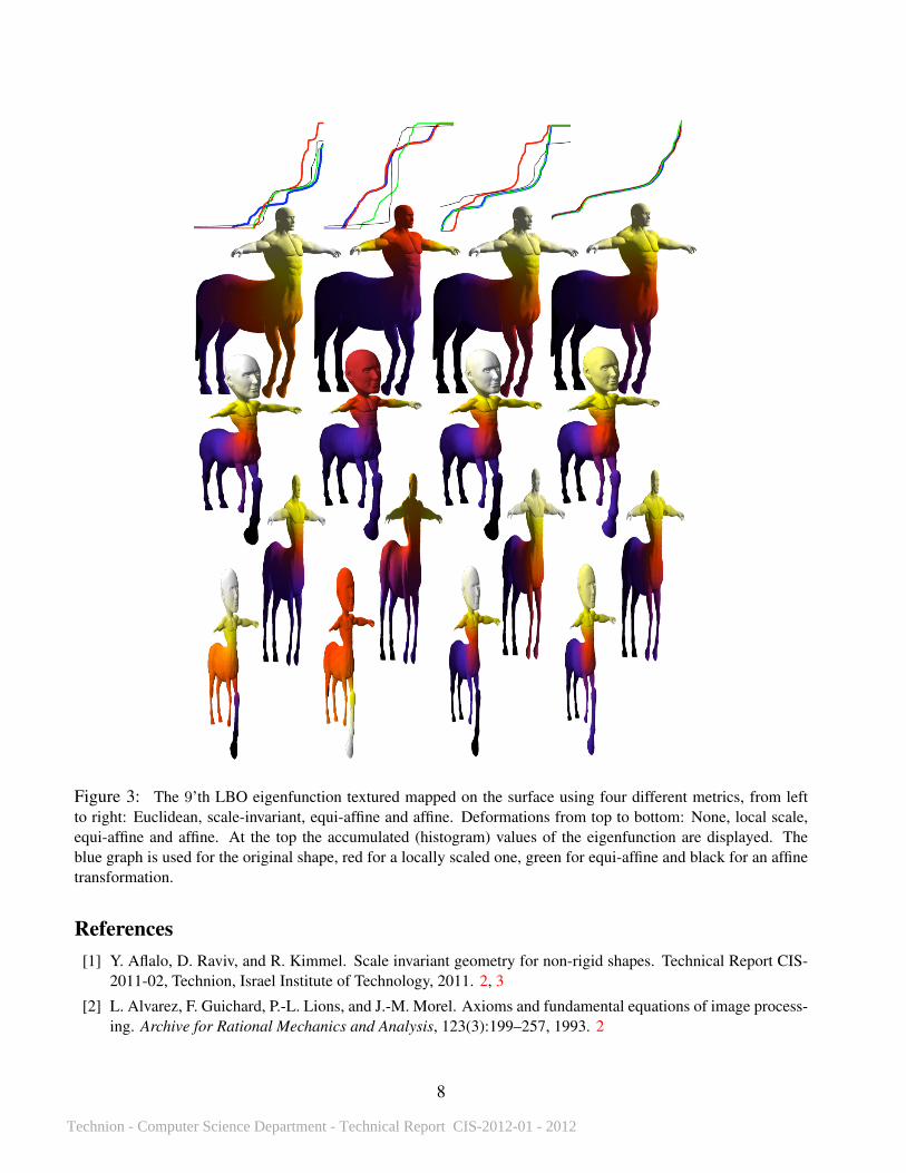
different metrics and different deformations. In Figure 3 we present the 9’th eigenfunction texturedmapped on the surface using an Euclidean metric, scale invariant metric, equi-affine metric and theproposed affine invariant metric. In each row a different deformation of the surface is presented. Onthe second row we applied local scaling, on the third row volume preserving stretching (equi-affine),and on the last row affine transformation (including local scale). At the top are plotted the accumulatedhistogram values of the eigenfunction. Blue color is used for the original shape, red for the locally scaledshape, green for the equi-affine transformed one, and black for the affine transformation.
In the second experiment, Figure 4, we evaluate the Heat Kernel Signatures of the surface subjectto local scaling, equi-affine and affine transformations, using the Euclidean and the affine metrics. Inaddition, we depict the accumulated values of the histograms, color coded as before.
In the third experiment, Figure 5 shows diffusion distances measured from the nose of a cat afteranisotropic scaling and stretching as well as an almost isomeric transformation.
Next, we compute Voronoi diagrams for ten points selected by the farthest point sampling strategy, asseen in Figures 6 and 1. Distances are measured with the global scale invariant commute time distances[41], and diffusion distances receptively, using a Euclidean metric and the proposed affine version.Again, the affine metric outperforms the Euclidean one.
In the next example we used the affine metric for finding the correspondence between two shapes. Weused the GMDS framework [7] with diffusion distances with the same initialization for both experiments.Figure 7 displays the Voronoi cells of matching surface segments.
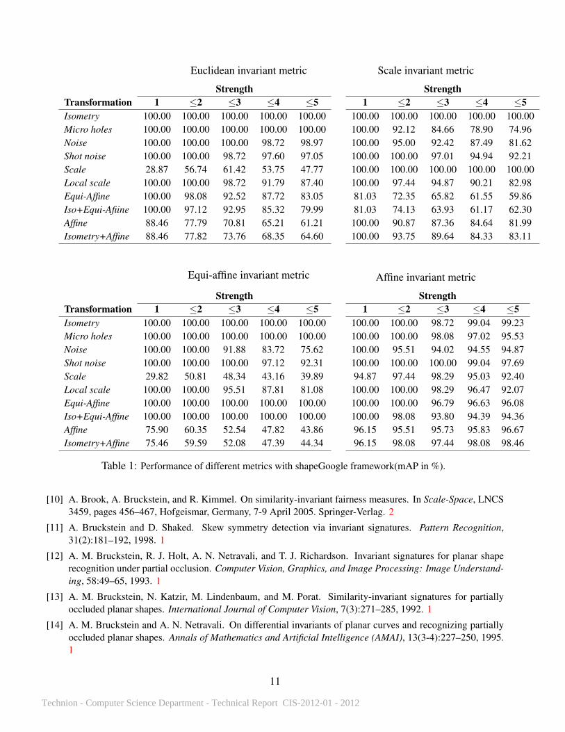
Finally, we evaluated the proposed metric on the SHREC 2010 dataset [6] using the shapeGoogleframework [37], after adding four new deformations; equi-affine, isometry and equi-affine, affine andisometry and affine. Table 1 shows that the new affine metric discriminative power is as good as theEuclidean one, performs well on scaling as the scale invariant metric, and similar to the the equi-affineone for volume preserving affine transformations. More over, the new metric is the only one capable tohandle full affine deformations added to SHREC dataset. Note that shapes which were considered locallyscaled in that database were in fact treated with an offset operation (morphological erosion) rather thanscaling. This explains some of the degradation in performances in the local scaled examples.
Performances were evaluated using precision/recall characteristic. Precision P(r) is defined as thepercentage of relevant shapes in the first r top-ranked retrieved shapes. Mean average precision (mAP),defined as mAP =
∑r P(r) · rel(r), where rel(r) is the relevance of a given rank, was used as a single
measure of performance. Intuitively, mAP is interpreted as the area below the precision-recall curve.Ideal retrieval performance (mAP=100%) is achieved when all queries return relevant first matches.Performance results were broken down according to transformation class and strength.
5. ConclusionsWe introduced a new metric that gracefully handles the affine group of transformations. Its differential
structure allows us to cope with local and global non-uniform stretching and scaling of the surfaces. Wedemonstrated that the proposed geometry and resulting computational methods could be useful for shapeanalysis like the SIFT and ASIFT operations were useful for image analysis.
Figure 3: The 9’th LBO eigenfunction textured mapped on the surface using four different metrics, from leftto right: Euclidean, scale-invariant, equi-affine and affine. Deformations from top to bottom: None, local scale,equi-affine and affine. At the top the accumulated (histogram) values of the eigenfunction are displayed. Theblue graph is used for the original shape, red for a locally scaled one, green for equi-affine and black for an affinetransformation.
References[1] Y. Aflalo, D. Raviv, and R. Kimmel. Scale invariant geometry for non-rigid shapes. Technical Report CIS-
2011-02, Technion, Israel Institute of Technology, 2011. 2, 3
[2] L. Alvarez, F. Guichard, P.-L. Lions, and J.-M. Morel. Axioms and fundamental equations of image process-ing. Archive for Rational Mechanics and Analysis, 123(3):199–257, 1993. 2
Figure 4: Affined heat kernel signatures for the regular metric (left), and the invariant version (right). The bluecircles represent the signatures for three points on the original surface, while the red plus signs are computed fromthe deformed version. Using a log-log axes we plot the scaled-HKS as a function of t.
Figure 5: Diffusion distances - Euclidean (left) and affine (right) - measured from the nose of the cat afternon-uniform scaling and stretching. The accumulated (histogram) distances (at the bottom) are color coded as inFigure 3.
[3] M. Andrade and T. Lewiner. Affine-invariant curvature estimators for implicit surfaces. Computer AidedGeometric Design, 29(2):162–173, 2012. 2
Figure 6: Voronoi diagrams using ten points selected by the farthest point sampling strategy. The commutetime distances were evaluated using the Euclidean metric (top) and the proposed affine one (bottom). We texturedmapped the result to the original mesh for comparison.
Figure 7: Correspondence search between two shapes using the GMDS [7] framework with diffusion distances.The affine (right) metric clearly outperforms the Euclidean one (left) in the presence of non-uniform stretching.Corollated surfaces segments have the same color.
[4] P. Berard, G. Besson, and S. Gallot. Embedding riemannian manifolds by their heat kernel. Geometric andFunctional Analysis, 4(4):373–398, 1994. 2
[5] W. Blaschke. Vorlesungen uber Differentialgeometrie und geometrische Grundlagen von Einsteins Relativi-tatstheorie, volume 2. Springer, 1923. 3
[6] A. M. Bronstein, M. M. Bronstein, U. Castellani, B. Falcidieno, A. Fusiello, A. Godil, L. J. Guibas, I. Kokki-nos, Z. Lian, M. Ovsjanikov, G. Patane, M. Spagnuolo, and R. Toldo. SHREC 2010: robust large-scale shaperetrieval benchmark. In Proc. 3DOR, 2010. 7
[7] A. M. Bronstein, M. M. Bronstein, and R. Kimmel. Efficient computation of isometry-invariant distancesbetween surfaces. SIAM J. Scientific Computing, 28(5):1812–1836, 2006. 2, 7, 10
[8] A. M. Bronstein, M. M. Bronstein, R. Kimmel, M. Mahmoudi, and G. Sapiro. A Gromov-Hausdorff frame-work with diffusion geometry for topologically-robust non-rigid shape matching. International Journal ofComputer Vision (IJCV), 89(2-3):266–286, 2010. 2
[9] M. M. Bronstein and I. Kokkinos. Scale-invariant heat kernel signatures for non-rigid shape recognition. InProc. Computer Vision and Pattern Recognition (CVPR), 2010. 2
Table 1: Performance of different metrics with shapeGoogle framework(mAP in %).
[10] A. Brook, A. Bruckstein, and R. Kimmel. On similarity-invariant fairness measures. In Scale-Space, LNCS3459, pages 456–467, Hofgeismar, Germany, 7-9 April 2005. Springer-Verlag. 2
[11] A. Bruckstein and D. Shaked. Skew symmetry detection via invariant signatures. Pattern Recognition,31(2):181–192, 1998. 1
[12] A. M. Bruckstein, R. J. Holt, A. N. Netravali, and T. J. Richardson. Invariant signatures for planar shaperecognition under partial occlusion. Computer Vision, Graphics, and Image Processing: Image Understand-ing, 58:49–65, 1993. 1
[13] A. M. Bruckstein, N. Katzir, M. Lindenbaum, and M. Porat. Similarity-invariant signatures for partiallyoccluded planar shapes. International Journal of Computer Vision, 7(3):271–285, 1992. 1
[14] A. M. Bruckstein and A. N. Netravali. On differential invariants of planar curves and recognizing partiallyoccluded planar shapes. Annals of Mathematics and Artificial Intelligence (AMAI), 13(3-4):227–250, 1995.1
[17] E. Calabi, P. Olver, C. Shakiban, A. Tannenbaum, and S. Haker. Differential and numerically invariantsignature curves applied to object recognition. International Journal of Computer Vision, 26:107–135, 1998.1
[18] S. Carlsson, R. Mohr, T. Moons, L. Morin, C. A. Rothwell, M. Van Diest, L. Van Gool, F. Veillon, andA. Zisserman. Semi-local projective invariants for the recognition of smooth plane curves. InternationalJournal of Computer Vision, 19(3):211–236, 1996. 2
[19] F. Chazal, D. Cohen-Steiner, L. Guibas, F. Memoli, and S. Oudot. Gromov-Hausdorff stable signatures forshapes using persistence. Computer Graphics Forum, 28(5):1393–1403, July 2009. 2
[20] T. Cohignac, C. Lopez, and J. Morel. Integral and local affine invariant parameter and application to shaperecognition. In Proceedings of the 12th IAPR International Conference on Pattern Recognition (ICPR),volume 1, pages 164–168, October 1994. 1
[21] R. R. Coifman, S. Lafon, A. B. Lee, M. Maggioni, B. Nadler, F. Warner, and S. W. Zucker. Geometric diffu-sions as a tool for harmonic analysis and structure definition of data: Diffusion maps. PNAS, 102(21):7426–7431, 2005. 2, 6
[22] M. P. do Carmo. Differential geometry of curves and surfaces. Prentice-Hall, 1976. 5
[23] G. Dziuk. Finite elements for the Beltrami operator on arbitrary surfaces. In S. Hildebrandt and R. Leis,editors, Partial differential equations and calculus of variations, pages 142–155. 1988. 6
[24] A. Elad and R. Kimmel. Bending invariant representations for surfaces. In Proc. Computer Vision andPattern Recognition (CVPR), pages 168–174, 2001. 2
[25] A. Gray, E. Abbena, and S. Salamon. Modern Differential Geometry of Curves and Surfaces with Mathe-matica. 3rd edition, 2006. 4
[26] A. Hamza and H. Krim. Geodesic matching of triangulated surfaces. IEEE Transactions on Image Process-ing, 15(8):2249–2258, 2006. 2
[27] R. Kimmel. Affine differential signatures for gray level images of planar shapes. In Proceedings of the 13thInternational Conference on Pattern Recognition, pages 45–49, vol. 1, Vienna, Austria, 25-30 August 1996.IEEE. 2
[28] H. Ling and D. Jacobs. Using the inner-distance for classification of articulated shapes. In Proc. ComputerVision and Pattern Recognition (CVPR), volume 2, pages 719–726, San Diego, USA, 20-26 June 2005. 2
[29] Y. Lipman and T. Funkhouser. Mobius voting for surface correspondence. In Proc. ACM Transactions onGraphics (SIGGRAPH), volume 28, 2009. 2
[30] D. Lowe. Distinctive image features from scale-invariant keypoint. International Journal of Computer Vision(IJCV), 60(2):91–110, 2004. 2
[31] F. Memoli and G. Sapiro. A theoretical and computational framework for isometry invariant recognition ofpoint cloud data. Foundations of Computational Mathematics, 5(3):313–347, 2005. 2
[32] M. Meyer, M. Desbrun, P. Schroder, and A. H. Barr. Discrete differential-geometry operators for triangulated2-manifolds. Visualization and Mathematics III, pages 35–57, 2003. 5
[33] T. Moons, E. Pauwels, L. Van Gool, and A. Oosterlinck. Foundations of semi-differential invariants. Inter-national Journal of Computer Vision (IJCV), 14(1):25–48, 1995. 2
[34] J. M. Morel and G.Yu. ASIFT: A new framework for fully affine invariant image comparison. Journal onImaging Sciences (SIAM), 2:438–469, 2009. 2
[35] P. Olver. A survey of moving frames. In H. Li, P. Olver, and G. Sommer, editors, Computer Algebra andGeometric Algebra with Applications, LNCS 3519, pages 105–138, New York, 2005. Springer-Verlag. 2
[36] P. J. Olver. Joint invariant signatures. Foundations of Computational Mathematics, 1:3–67, 1999. 2
[37] M. Ovsjanikov, A. M. Bronstein, M. M. Bronstein, and L. J. Guibas. Shape Google: a computer visionapproach to invariant shape retrieval. In Proc. Non-Rigid Shape Analysis and Deformable Image Alignment(NORDIA), 2009. 2, 7
[38] M. Ovsjanikov, Q. Merigot, F. Memoli, and L. J. Guibas. One point isometric matching with the heat kernel.Proc. Symposium on Geometry Processing (SGP), 29(5):1555–1564, Jul 2010. 2
[39] E. Pauwels, T. Moons, L. Van Gool, P. Kempenaers, and A. Oosterlinck. Recognition of planar shapes underaffine distortion. International Journal of Computer Vision (IJCV), 14(1):49–65, 1995. 2
[40] K. Polthier and M. Schmies. Straightest geodesics on polyhedral surfaces. Mathematical Visualization, 1998.5
[41] H. Qiu and E. Hancock. Clustering and embedding using commute times. IEEE Transactions on PatternAnalysis and Machine Intelligence, 29(11):1873–1890, November 2007. 7
[42] D. Raviv, A. M. Bronstein, M. M. Bronstein, R. Kimmel, and N. Sochen. Affine-invariant diffusion geometryof deformable 3D shapes. In Proc. Computer Vision and Pattern Recognition (CVPR), 2011. 2, 3, 6
[43] R. Rustamov. Laplace-Beltrami eigenfunctions for deformation invariant shape representation. In Proc.Symposium on Geometry Processing (SGP), pages 225–233, 2007. 2
[45] J. Sun, M. Ovsjanikov, and L. J. Guibas. A concise and provably informative multi-scale signature based onheat diffusion. In Proc. Symposium on Geometry Processing (SGP), 2009. 2, 6
[46] L. Van Gool, M. Brill, E. Barrett, T. Moons, and E. Pauwels. Semi-differential invariants for nonplanarcurves. In J. Mundy and A. Zisserman, editors, Geometric Invariance in Computer Vision, pages Chapter11: 293–309, Massachusetts / London, Englad, 1992. MIT Press: Cambridge. 2
[47] L. Van Gool, T. Moons, E. Pauwels, and A. Oosterlinck. Semi-differential invariants. In J. Mundy andA. Zisserman, editors, Geometric Invariance in Computer Vision, pages Chapter 8: 157–192, Massachusetts/ London, England, 1992. MIT Press: Cambridge. 2
[48] Y. Wang, M. Gupta, S. Zhang, S. Wang, X. Gu, D. Samaras, and P. Huang. High resolution tracking of non-rigid motion of densely sampled 3D data using harmonic maps. International Journal of Computer Vision(IJCV), 76(3):283–300, 2008. 2
[49] I. Weiss. Projective invariants of shapes. Technical Report CAR-TR-339, University of Maryland - Centerfor Automation, January 1988. 1