P/E and PRICE-to-BOOK RATIOS as PREDICTORS of STOCK RETURNS IN EMERGING EQUITY MARKETS Kürşat Aydoğan Faculty of Business Administration Bilkent University Bilkent, 06533 Ankara, TURKEY E-mail: [email protected]and Güner Gürsoy ∗ Faculty of Business Administration BilkentUniversity Bilkent 06533 Ankara, TURKEY E-mail: [email protected]August 2000 ∗ Corresponding Author
Transcript
P/E and PRICE-to-BOOK RATIOS as PREDICTORS of STOCK RETURNS IN EMERGING EQUITY MARKETS
P/E and PRICE-to-BOOK RATIOS as PREDICTORS of STOCK RETURNS IN EMERGING EQUITY MARKETS
Recent research in empirical finance has shown that variables like dividend yields, price-
to-earnings (P/E) ratios, book-to-market ratios as well as past returns have significant
explanatory power for the variation in cross section of expected returns even after controlling
for market risk (see, for example, Fama and French, 1992, for a through coverage of the topic).
Similar results are reported for several developed markets (Ferson and Harvey, 1997; Fama
and French, 1998), as well as emerging markets (Bekaeert, et. al., 1997; Claessens, Dasgupta
and Glen, 1998; Patel, 1998; Rouwenhorst, 1999). Whether these variables are risk proxies in
an efficient market or signs of mispricing is the subject an ongoing debate in financial
economics. Yet for the practitioner in the market, it is the longer term predictive ability, rather
than contemporaneous explanatory power, that is really important. In addition, apart from
forecasting individual stock returns, stock market investors are also interested in the
forecasting power of market wide averages of variables like dividend yield, P/E and book-to-
market ratios as tools in market timing in highly volatile stock markets. The objective of this
paper is to investigate the ability of average P/E and book-to-market ratios to predict future
stock market returns in emerging equity markets. Emerging markets are differentiated from
developed markets with respect to their heterogeneous nature and inherent dynamics. These
are the markets characterized by high volatility and high average returns. It has been shown
that they are not integrated to the developed markets of the World as evidenced by very low
correlation with the rest of the World and among themselves [Bekaert et. al., 1998]. Hence the
importance of market timing and country selection for an internationally diversified portfolio
investor is obvious. Achour et. al. [1998] stresses the importance of country selection
1
mechanisms as well as stock selection. Erb, Harvey and Viskanta [1995], on the other hand,
argue that selection based on country risk rather than traditional attributes such as P/E,
dividend yield and book-to-market yields superior results in emerging markets.
Following the earlier research in 1960's and 1970's, which in general support the view
that stock returns could not be predicted, more recent studies provide evidence that medium to
long term stock returns can be explained by variables like dividend yields, price earnings
ratios, term structure, default premiums and past returns (see, for example, Fama and French,
1988 and 1989, Campbell and Schiller, 1988). These findings seem to contradict efficient
markets hypothesis. Yet Fama [1991] argues that return predictability is the result of changing
expected returns over time, rather then a sign of inefficiency. Investigating the sources of
predictability in stock returns, Ferson and Harvey [1991] find that, rather than inefficiencies
like fads; it is the change in expected returns and risk sensitivities (betas) that explain
predictable component of stock returns. Harvey [1995] asserts that emerging market returns
are more predictable than developed market returns.
Return predictability does not necessarily give way to excess profits in the market. In
their general equilibrium model that yields predictable stock returns, Balvers, Cosimano and
McDonald [1990] suggest that advantages of predictive ability are offset by fluctuations in
consumption patterns. Empirically, Fuller and Kling [1994] cannot uncover any evidence for
superior profits using return prediction models. As pointed out by Fama [1991], their finding
is not surprising in the light of the "poor statistical power" of such models.
Blieberg [1994] employs aggregate data for future stock returns and average P/E ratio
to develop a market timing and asset allocation strategy. To this end, he groups historical
average P/E ratios into quintiles and relates them with future returns using S&P 500 index. In
2
this paper, we initially adopt a similar approach by grouping observed average P/E and book-
to-market ratios (PBV) into quintiles in 19 emerging equity markets and associating them with
3-month, 6-month and 12-month ahead future returns. We also perform econometric tests on
the panel data of emerging equity markets for the period between 1986 to 1999 Our results
indicate that both P/E and book-to-market ratios have predictive power of future return,
especially over longer time periods, hence can be used as tools in forming a market timing and
asset allocation strategy in emerging equity markets.
The organization of the paper is as follows. Section two describes the data. Results of
simple grouping with respect to P/E and book-to-market ratios are given in Section 3.
Econometric tests are presented in Section 4. Summary and concluding remarks are presented
in the final section.
DATA
Our study is confined to a group of countries widely known as "emerging equity
markets" defined and monitored by International Finance Corporation (IFC) arm of the World
Bank. IFC reports market wide data on these countries in its publication titled "Annual
Factbook”. We obtained end of month national average market P/E and price-to-book (PBV)
ratios, as well as values of the national market indices and exchange rates from IFC Annual
Factbook for years between 1986 and 1999. National market indices are value weighted and
they account for a significant portion of total market capitalization in each country. Financial
Times World Index, used to calculate country betas, is obtained from Datastream. Our data
set spans from January 1986 to December 1999. In order to deal with the numerical problems
inherent in the definition of P/E ratio, we chose to work with its reciprocal, the ratio of
3
earnings to price, or E/P ratio. In most of the analysis that follows, we discarded observations
with negative E/P values.
To compute the monthly rate of return, Rt, in a market, we first express the local
market index in US dollars and calculate the percentage change in the dollar denominated
index, I, from month t-1 to month t.
We present summary statistics for monthly dollar returns, Rt, E/P and PBV for all the
countries in the sample in Exhibit 1. Variation across countries and within country variation
for all variables are remarkable. For example, simple average monthly dollar rate of return in
emerging equity markets is 1.3% with a standard deviation of 12.2%. Same figures for
Financial Times World (FTW) index, which heavily reflects developed capital markets, is
0.83% and 4.24% respectively. When Pearson correlations between stock market returns in
individual countries are examined (not reported), very low correlation is found. This finding
indicates a low level of integration within the group, as well as with the developed markets, as
shown by low level of correlation with FTW index, in general.
INSERT EXHIBIT 1 HERE
E/P RATIO AND STOCK RETURNS
We first compute 3-month, 6-month and 12-month ahead returns in each stock market
in month t by taking that month as the starting period. Hence the 3, 6 and 12 month ahead
returns, Rt, t+j, are found as percentage changes in the local market index expressed in US
dollars, I, in the following manner:
4
)1(12,6,3, =−
= ++ jfor
III
Rt
tjtjtt
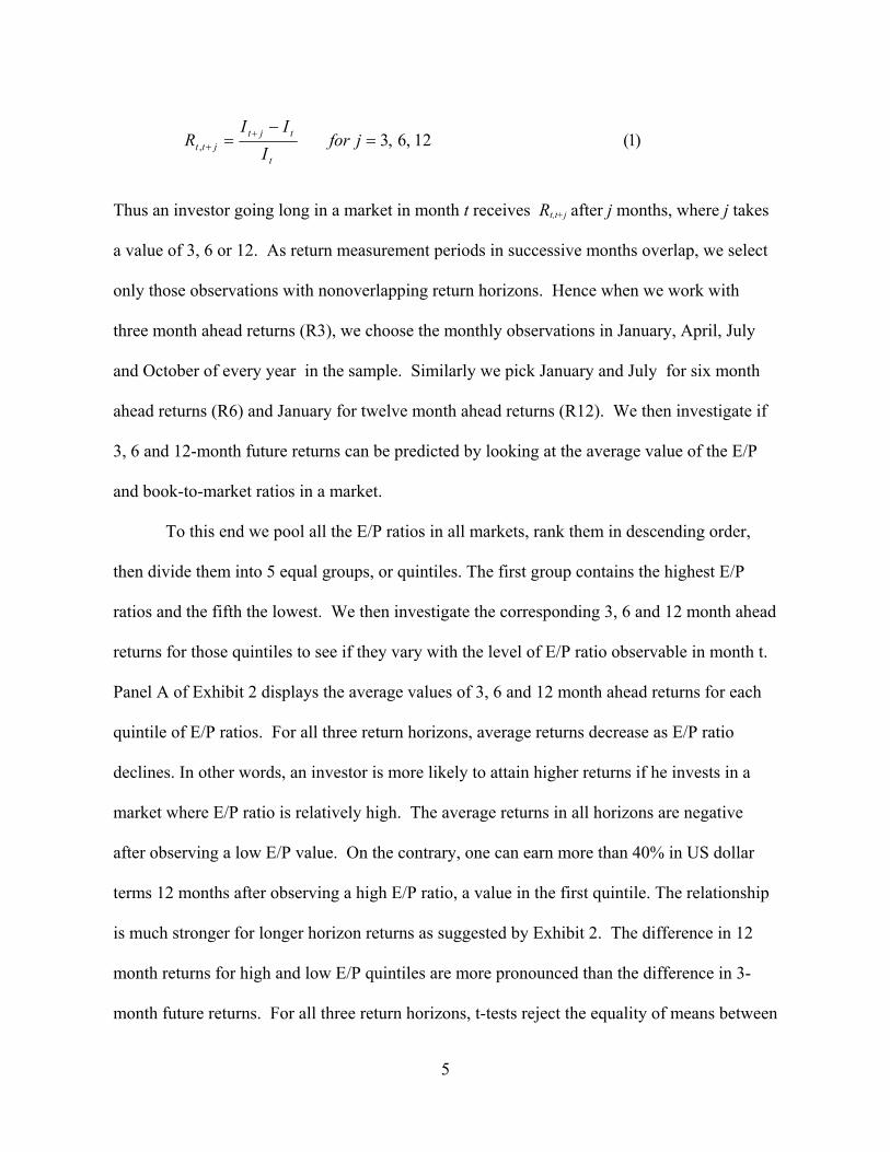
Thus an investor going long in a market in month t receives Rt,t+j after j months, where j takes
a value of 3, 6 or 12. As return measurement periods in successive months overlap, we select
only those observations with nonoverlapping return horizons. Hence when we work with
three month ahead returns (R3), we choose the monthly observations in January, April, July
and October of every year in the sample. Similarly we pick January and July for six month
ahead returns (R6) and January for twelve month ahead returns (R12). We then investigate if
3, 6 and 12-month future returns can be predicted by looking at the average value of the E/P
and book-to-market ratios in a market.
To this end we pool all the E/P ratios in all markets, rank them in descending order,
then divide them into 5 equal groups, or quintiles. The first group contains the highest E/P
ratios and the fifth the lowest. We then investigate the corresponding 3, 6 and 12 month ahead
returns for those quintiles to see if they vary with the level of E/P ratio observable in month t.
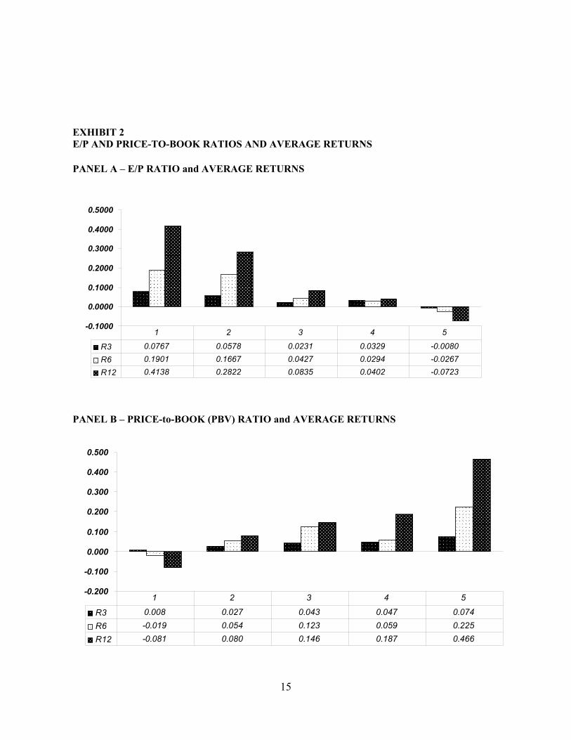
Panel A of Exhibit 2 displays the average values of 3, 6 and 12 month ahead returns for each
quintile of E/P ratios. For all three return horizons, average returns decrease as E/P ratio
declines. In other words, an investor is more likely to attain higher returns if he invests in a
market where E/P ratio is relatively high. The average returns in all horizons are negative
after observing a low E/P value. On the contrary, one can earn more than 40% in US dollar
terms 12 months after observing a high E/P ratio, a value in the first quintile. The relationship
is much stronger for longer horizon returns as suggested by Exhibit 2. The difference in 12
month returns for high and low E/P quintiles are more pronounced than the difference in 3-
month future returns. For all three return horizons, t-tests reject the equality of means between
5
E/P quintiles. However, in shorter horizons, the difference between average returns for two
adjacent quintiles are not always significantly different from zero, and it may even be negative
as in the case of the 3 month ahead returns for the third and fourth E/P quintiles. Similar
analysis using price-to-book ratios yield more striking results. As shown in Panel B of
Exhibit 2, average returns monotonically increase with the price-to-book quintile for each
return horizon. The difference in 12 month ahead returns between lowest and highest book-to-
market quintiles is more than 45%.
INSERT EXHIBIT 2 HERE
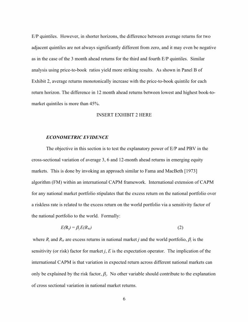
ECONOMETRIC EVIDENCE
The objective in this section is to test the explanatory power of E/P and PBV in the
cross-sectional variation of average 3, 6 and 12-month ahead returns in emerging equity
markets. This is done by invoking an approach similar to Fama and MacBeth [1973]
algorithm (FM) within an international CAPM framework. International extension of CAPM
for any national market portfolio stipulates that the excess return on the national portfolio over
a riskless rate is related to the excess return on the world portfolio via a sensitivity factor of
the national portfolio to the world. Formally:
E(Rj) = βj E(RW) (2)
where Rj and RW are excess returns in national market j and the world portfolio, βj is the
sensitivity (or risk) factor for market j, E is the expectation operator. The implication of the
international CAPM is that variation in expected return across different national markets can
only be explained by the risk factor, βj. No other variable should contribute to the explanation
of cross sectional variation in national market returns.
6
We employ the above framework to test the explanatory power of E/P and PBV in
future returns by taking risk sensitivity of the market into consideration. Bekaert et. al. [1998]
suggests that the predictability power can be best captured by regression models because of
the time varying characteristic of mean returns. First a time series regression is run for each
national market to estimate the risk factor using the first 24 monthly observations, between
April 86 and March 88:
Rjt = αj + βjRWt + εt (3)
where Rjt is the return in market j in month t, RWt is the return on the world portfolio in month
t, αj , βj are the coefficients, and εt is the error term. At the end of this stage we have a set of
19 β estimates, one for each country in the sample. Then, using the cross section of
observations for the 25th month, i.e. April 88, we estimate the following regression models via
OLS to test the explanatory power of E/P and PBV on future returns where βs are also
included to control risk differences1:
Ri = λ0 + λ1 EPi + λ2 βi + εi (4)
Ri = λ0 + λ3 PBVi + λ2 βi + εi (5)
Ri = λ0 + λ1 EPi + λ2 βi + λ3 PBVi + εi (6)
where Ri = 3, 6 or 12 month ahead returns in national market i, EPi is the average earnings to
price ratio in market i, PBVi is the book-to-market ratio in market i, λs are regression
coefficients, and ε's are error terms. Each model is estimated for all three return horizons, i.e.
3, 6 and 12-month future returns. We repeat the same process for each non overlapping time
period between April 88 and December 1999 by updating β estimates every time. For
7
example, for the estimation of July1988, a β value for each market is found by utilizing time
series of observations between May 86 and June 88 in the second model as specified in
equation 3, together with E/P and PBV from July 1988. Hence, depending on the return
horizon, each equation is estimated 12-47 times, yielding a set of estimates for the regression
coefficients in (4) – (6). We are interested to see if coefficients (λs ) of E/P and PBV are
different from zero. A t-test on the mean value of the time series of estimated coefficients
provide the necessary answer. Rejection of the null hypotheses of zero means for these
coefficients would lead to the conclusion that E/P and PBV have explanatory power of future
returns even after controlling for risk.
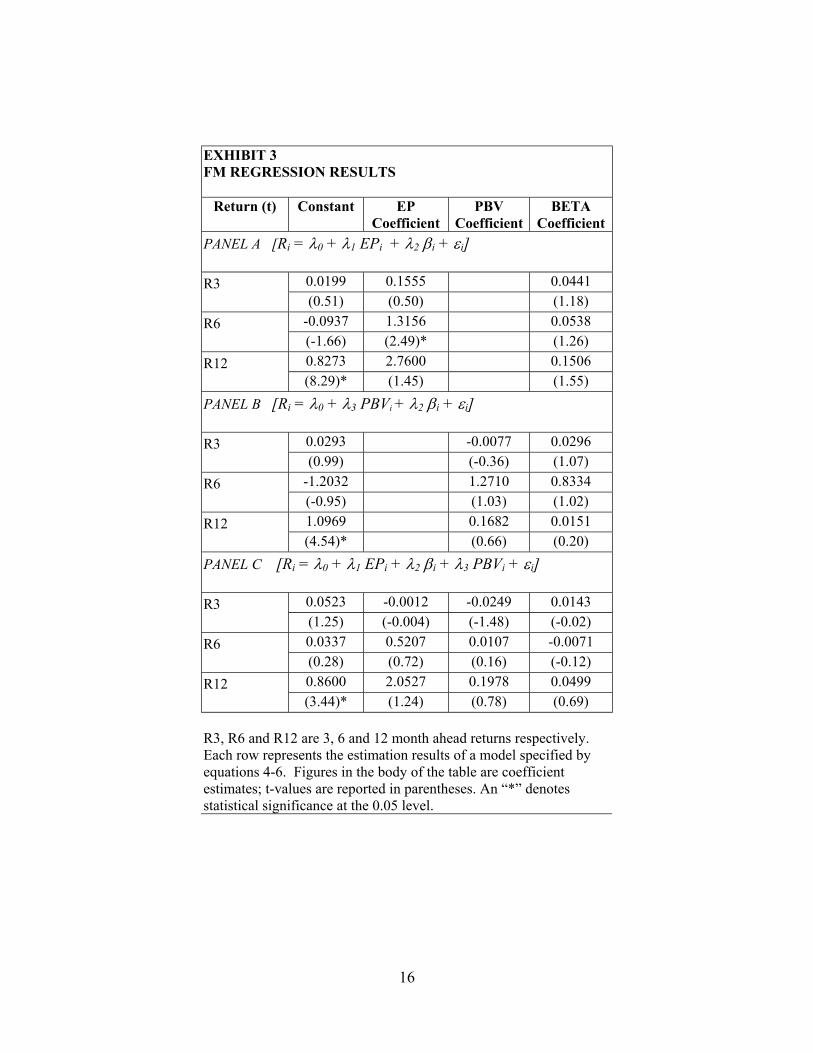
Results are presented in Exhibit 3. One interesting finding in all the models is the lack
of significance of the coefficient of the risk variable, β. Although surprising in terms of the
implications of international CAPM, lack of significance of the risk variable is hardly a new
empirical phenomenon. In fact in most recent tests of the CAPM, failure of a significant
coefficient for the beta risk is very common, albeit in US markets, e.g. Fama and French
[1992]. In the international setting, Harvey [1991] finds that world risk exposure can only
partially explain the cross-sectional return differences among developed countries. In
emerging markets, Rouwenhorst [1999] finds that high beta stocks do not outperform low beta
stocks.
Estimation results for equation (4) above are given in the first panel of Exhibit 3. This
model tests the impact of E/P ratio on future returns. For longer return horizons, coefficient
for the E/P variable is significant. Higher E/P ratios in the market lead to higher returns
1 We also employed weighted least squares in the estimation of (4)-(6), where residual standard deviations in time series estimation of country betas are used as weights in cross sectional regressions. Results (not reported) are essentially similar.
8
subsequently. The second model as specified in equation (5), which tests the impact of PBV,
is presented in the second panel. Here, the coefficients for the variable of interest carry the
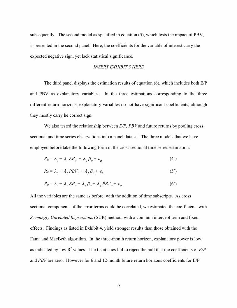
The third panel displays the estimation results of equation (6), which includes both E/P
and PBV as explanatory variables. In the three estimations corresponding to the three
different return horizons, explanatory variables do not have significant coefficients, although
they mostly carry he correct sign.
We also tested the relationship between E/P, PBV and future returns by pooling cross
sectional and time series observations into a panel data set. The three models that we have
employed before take the following form in the cross sectional time series estimation:
Rit = λ0 + λ1 EPit + λ2 βit + εit (4´)
Rit = λ0 + λ1 PBVit + λ2 βit + εit (5´)
Rit = λ0 + λ1 EPit + λ2 βit + λ3 PBVit + εit (6´)
All the variables are the same as before, with the addition of time subscripts. As cross
sectional components of the error terms could be correlated, we estimated the coefficients with
Seemingly Unrelated Regressions (SUR) method, with a common intercept term and fixed
effects. Findings as listed in Exhibit 4, yield stronger results than those obtained with the
Fama and MacBeth algorithm. In the three-month return horizon, explanatory power is low,
as indicated by low R2 values. The t-statistics fail to reject the null that the coefficients of E/P
and PBV are zero. However for 6 and 12-month future return horizons coefficients for E/P
9
and PBV are significant with expected signs in all three panels. The risk variable, β, still lacks
significance in 8 of the 9 models estimated.
INSERT EXHIBIT 4 HERE
SUMMARY AND CONCLUDING REMARKS
This paper is an attempt to uncover tools like E/P and PBV ratios to forecast longer
horizon average market returns in emerging equity markets. We pool market averages of E/P
and PBV for all emerging equity markets and try to see if they are related with 3, 6 and 12-
month future returns. First, we rank the pooled observations with respect to E/P (PBV) and
group them into quintiles. When we relate grouped E/P (PBV) values to future returns, we
find that returns are higher after observing a high E/P (low PBV) in a market. Two sets of
econometric tests are invoked to test the statistical relationship between E/P, PBV and future
returns. Initially, we employ Fama and MacBeth’s methodology to control for worldwide risk
in an international CAPM framework. Next, we undertake a time series - cross sectional
estimation of international CAPM models. Although FM method does not provide significant
coefficients, E/P and PBV appear to predict future returns in pooled estimation. However,
explanatory powers are very low in shorter return horizons.
The fact that fundamental variables are related with future returns in less developed,
diverse markets have strong implications for asset pricing in general. These variables have
been shown to explain cross section of expected returns in developed markets. Yet they do not
easily lend themselves to a model of capital market equilibrium; such findings are still
regarded as an empirical regularity yet to be explained. Similar phenomenon in emerging
equity markets is not therefore very puzzling. In terms of forecasting ability, the relationship
10
between E/P, PBV and future returns are encouraging, but not very promising for the potential
investor. One has only got to consider the low explanatory power of the models estimated in
this study.
11
REFERENCES
Achour D., Harvey C. R., Hopkins G., and Lang C. “Stock Selection in Emerging Markets: Portfolio Strategies for Malaysia, Mexico, and South Africa.” Emerging Markets Quarterly, Winter 1998, pp. 38-91.
Balvers, R. J., T. E. Cosamino, and MacDonald. “Predicting Stock Returns in an Efficient
Market.” Journal of Finance, 1990, 43, pp. 661-676. Bekaert, Geert, C. B. Erb, C. R. Harvey and T. E. Viskanta, “The Cross-Sectional
Determinants of Emerging Market Equity Returns.” in Carman, Peter, Ed., Quantitative Investing for the Global Markets, Glenlake, 1997.
Bekaert G., Harvey C. R., Erb C., and Viskanta T. The Behavior of Emerging Market Returns
in The Future of Emerging Market Capital Flows, Richard Levich (ed.), Boston: Kluwer Academic Publishers, 1998, pp. 107-173.
Bleiberg, Steven . “Price-earnings ratios as a valuation tool”, in Lofthouse, Stephen, Readings
in Investments, Wiley, 1994, pp. 341-351. Campbell, John Y., and R. J. Shiller. “Stock Prices, Earnings, and Expected Dividends.”
Journal of Finance, 1988, 48, pp. 661-676. Claessens, Stijn S. Dasgupta, and J. Glen, “The Cross Section of Stock Returns: Evidence
from Emerging Markets.” Emerging Markets Quarterly, 1998, 2, pp. 4-13. Erb, Claude B, C. R. Harvey, and T. E. Viskanta, “Country Risk and Global Equity Selection.”
Journal of Portfolio Management, 1995, 21, pp. 74-81. Fama, Eugene. “Efficient Capital Markets: II.” Journal of Finance, 1991, 46, pp. 1575-1617. Fama, Eugene, and K. R. French. “Dividend Yields and Expected Stock Returns.” Journal of
Financial Economics, 1988, 22, pp. 3-25. Fama, Eugene, and K. R. French. “Business Conditions and Expected Returns on Stocks and
Bonds.” Journal of Financial Economics, 1989, 25, pp. 23-49. Fama, Eugene and French, Keneth R. “The Cross-Section of Expected Returns.” Journal of
Finance, 1992, 47, pp. 427-466. Fama, Eugene and French, Keneth R. “Value versus Growth: The International Evidence.”
Journal of Finance, 1998, 53, pp. 1975-1999. Fama, Eugene and J. Macbeth. “Risk, Return and Equilibrium: Empirical Tests.” Journal of
Political Economy, 1991, 81, pp. 607-636.
12
Ferson, Wayne E., and C. R. Harvey. “Sources Of Predictability In Portfolio Returns.”
Financial Analysts Journal, 1991, 47, pp. 49-61. Ferson, Wayne E., and C. R. Harvey. “Fundamental Determinants of National Equity Market
Returns: A Perspective on Conditional Asset Pricing.” Journal of Banking and Finance, 1997, 21, pp. 1625-1665.
Fulller, Russell J. and John L. King. “Can Regression-Based Models Predict Stock and Bond
Returns?” Journal of Portfolio Management, Spring 1994, pp. 56-63. Harvey Campbell R., “Predictable Risk and Returns In Emerging Markets.” Review of
Financial Studies, 1995, pp. 773-816. Harvey Campbell R., “The World Price of Covariance Risk.” Journal of Finance, 1991, 46,
pp. 111-157. International Finance Corporation Annual Factbooks 1985-1997. Patel, Sandeep A., “Cross-sectional Variation in Emerging Markets Equity Returns; January
1988-March 1997.” Emerging Markets Quarterly, 1998, 2, pp. 57-70. Rouwenhorst, K. Geert, “Local Return Factors and Turnover in Emerging Stock Markets.”
Journal of Finance, 1999, 54, pp. 1439-1464.
13
EXHIBIT 1 SUMMARY STATISTICS FOR EMERGING MARKETS
Average Monthly Return
Earnings to Price (E/P)
Price to Book Value (PBV)
Pearson Correlation
Countries Mean Standard Deviation
Mean Standard Deviation
Mean Standard Deviation
Corr. Sig. (2-tailed)
Argentina 0.023 0.173 0.098 0.189 1.326 1.118 0.028 0.785 Chile 0.019 0.074 0.116 0.085 1.462 0.604 0.142 0.129 Colombia 0.009 0.116 0.098 0.052 1.099 0.526 0.009 0.924 Greece 0.025 0.119 0.077 0.034 2.695 1.667 0.159 0.090 India 0.004 0.109 0.058 0.022 3.029 1.286 -0.102 0.265 Indonesia 0.001 0.135 0.053 0.018 2.520 0.953 0.102 0.372 Jordan 0.000 0.047 0.075 0.020 1.579 0.218 0.056 0.544 Korea 0.016 0.117 0.048 0.015 1.414 0.558 0.303* 0.001 Malaysia 0.011 0.106 0.043 0.019 2.594 0.986 0.512* 0.000 Mexico 0.031 0.133 0.099 0.066 1.485 0.600 0.317* 0.001 Nigeria 0.007 0.141 0.138 0.044 2.077 0.737 0.085 0.355 Pakistan 0.000 0.101 0.149 0.216 2.055 0.898 0.102 0.262 Philippines -0.004 0.126 0.065 0.022 2.938 0.957 0.315* 0.001 Taiwan 0.011 0.113 0.063 0.021 2.457 1.432 0.408* 0.000 Thailand 0.024 0.136 0.041 0.018 3.948 2.792 0.296* 0.001 Turkey 0.013 0.131 0.074 0.026 2.253 0.981 -0.104 0.253 Venezuela 0.034 0.191 0.096 0.077 4.040 1.932 0.006 0.952 Zimbabwe 0.014 0.148 0.096 0.062 1.777 0.918 -0.045 0.632 Portugal 0.010 0.096 0.177 0.093 1.374 0.610 -0.016 0.868 Average 0.013 0.122 0.088 0.058 2.217 1.041 Mean and standard deviation values of (1) Average monthly returns; (2) Earnings to price ratio; (3) Price to book value ratio for 19 countries in the sample. Pearson correlations of individual emerging equity market returns with FTW Index return are reported in the last two columns (Significant correlations at the 0.05 level are marked with “*”)
14
EXHIBIT 2 E/P AND PRICE-TO-BOOK RATIOS AND AVERAGE RETURNS PANEL A – E/P RATIO and AVERAGE RETURNS
R3, R6 and R12 are 3, 6 and 12 month ahead returns respectively. Each row represents the estimation results of a model specified by equations 4-6. Figures in the body of the table are coefficient estimates; t-values are reported in parentheses. An “*” denotes statistical significance at the 0.05 level.
(54.05)* (5.77)* (-10.80)* (0.74) R3, R6 and R12 are 3, 6 and 12 month ahead returns respectively. Each row represents the estimation results of a model specified in equations 4´- 6´. Figures in the body of the table are coefficient estimates; t-values are reported in parentheses. An “*” denotes statistical significance at the 0.05 level.