Performance Comparison of Two Virtual Machine Scenarios Usingan HPC Application
A Case study Using Molecular Dynamics Simulations
Anand Tikotekar, Hong Ong, Sadaf Alam, Geoffroy Vallée,Thomas Naughton, Christian Engelmann & Stephen L. Scott ∗
Computer Science and Mathematics DivisionOak Ridge National Laboratory
Oak Ridge, TN, USA.
AbstractObtaining high flexibility to performance-loss ratio is a keychallenge of today’s HPC virtual environment landscape.And while extensive research has been targeted at extract-ing more performance from virtual machines, the idea thatwhether novel virtual machine usage scenarios could lead tohigh flexibility Vs performance trade-off has received lessattention.
We, in this paper, take a step forward by studying andcomparing the performance implications of running theLarge-scale Atomic/Molecular Massively Parallel Simula-tor (LAMMPS) application on two virtual machine configu-rations. First configuration consists of two virtual machinesper node with 1 application process per virtual machine. Thesecond configuration consists of 1 virtual machine per nodewith 2 processes per virtual machine. Xen has been used asan hypervisor and standard linux as a guest virtual machine.Our results show that the difference in overall performanceimpact on LAMMPS between the two virtual machine con-figurations described above is around 3%. We also study thedifference in performance impact in terms of each configu-ration’s individual metrics such as CPU, I/O, Memory, andinterrupt/context switches.
∗ORNL’s work was supported by the U.S. Department of Energy, underContract DE-AC05-00OR22725.
Permission to make digital or hard copies of all or part of this work for personal orclassroom use is granted without fee provided that copies are not made or distributedfor profit or commercial advantage and that copies bear this notice and the full citationon the first page. To copy otherwise, to republish, to post on servers or to redistributeto lists, requires prior specific permission and/or a fee.
1. IntroductionHigh-performance computing is increasingly leveraging vir-tualization due to its flexibility, such as the ability to per-form fault-tolerance using live migration, the ability to ef-ficiently allocate resources, the customizability according toapplication requirements, etc. Yet, such flexibility cannot of-ten offset the performance overhead of using virtualizationsolutions. To alleviate this trade-off between the flexibilityoffered and the generated performance hit, many in the HPCcommunity have looked at solutions that optimize hyper-visors, kernels, I/O, etc. And while this vertical optimiza-tion is certainly helpful, no such extensive research is beingextended to the efficacious use of virtual machines them-selves. After all, virtual machines are nothing if not mal-leable. Therefore, it seems reasonable to think that a novelconfiguration of virtual machines could end up providing afavorable trade-off between flexibility and the performanceimpact. For example, based on an application’s communica-tion pattern, communicating virtual machines could be kepton the same nodes to free more nodes as spare nodes forfault-tolerance. Another configuration design option is to de-cide whether to create a separate domain for a monitoringthread or add the thread to an existing domain. Many othervirtual machine configurations such as efficient resource al-location of memory may be costly from a performance pointof view due to additional memory pressure, but can providecertain flexibility by allowing to host another light-weightvirtual machine that uses idle time of the running applica-tion for check pointing. The idea thus is to employ a vir-tual machine configuration for which the “ratio of flexibil-ity” offered to the performance impact is high. Two logicalquestions arise: One, how to quantify the difference betweenthe flexibility offered by two virtual machine configurations?Second, what, if any, is the performance impact between twovirtual machine configurations? Please note that all the dis-cussion pertains to a fixed run of an application instance.
In this paper, we try to tackle the simpler of the twoquestions, which is about the performance impact. We haveselected the following two virtual machine configurations.Configuration 1 consists of two virtual machines per nodewith 1 application process per virtual machine. Configura-tion 2 consists of 1 virtual machine per node with 2 pro-cesses per virtual machine. Please note that we are not claim-ing that these configurations are suitable for this instance ofLAMMPS application. We only want to highlight the differ-ence, if any, in the performance impact between these con-figurations as they do the same amount of work.
Our contributions in this paper are the following: Weadvocate the idea that virtual machines could be used innovel ways so as to benefit the flexibility versus performanceimpact equation. Second, we study the performance impactof two virtual machine configurations on LAMMPS (12),and report the overall as well detailed performance impactof each configuration.
2. Related WorkResearchers in HPC domain have mainly focused on bring-ing down the performance overhead of virtualization. To-wards this end, the research is focused on efficient hyper-visors such as Xen (2). Efficient I/O solutions are advocatedin (6), (8), (17) that seek to minimize the I/O overheadof virtualization. Many other research efforts focus on usinglightweight domains (16), microkernels (3), and lightweightkernels (15) to reduce the cost of the hypervisor itself. Manystudies have evaluated the performance impact of virtualiza-tion on HPC applications. Such studies include (18), (9),(5). The common conclusion is that Xen is efficient in exe-cuting HPC applications.The flexibility aspect of virtualiza-tion is mainly exploited for fault tolerance (10), (11) in HPC.
Grid computing has leveraged various usage and execu-tion models of virtual machines. Vmplants (7) provides au-tomatic configuration of virtual machines to meet variousapplication requirements. Other studies for resource provi-sioning in grids include (14).
The idea of determining whether novel virtual machineusage scenarios, configurations could lead to better flexibil-ity vs performance-loss ratio in HPC has not been exploredin detail. Authors in (13) study whether intelligent managentof virtual machines could improve the utilization of physicalresources or not. Authors in (4) compare their distributedsystem MemX on three modes within Xen vm. These modesinclude driver domain, and individual guest domain. In thispaper we compare two virtual machine configurations thatare similar to each other. In the paper (1), authors study thenetwork processing overheads in Xen on two configurations.Their configurations include running I/O service vm and theguest vm on the same CPU, and on a different CPU. The au-thors are interested in comparing the network performancein these two modes with the native mode. Our study dealswith determining if there is any impact on an HPC applica-
tion when subjected to two similar virtual machine configu-rations.
3. Experimentation Description3.1 Hardware and SoftwareWe have used Xen 3.0.4 and linux kernel version 2.6.16.33with FC5 distribution and NFS filesystem. Our cluster con-sists of 16 nodes each with 2GHz processor with 768MBRAM. Both of our virtual machine configurations use Xenas their hypervisor and para-virtualized linux as their guestoperating system. Xen is responsible for domain schedul-ing, aggregating domain I/O requests and responses, mem-ory handling between domains, etc. Thus, it is easy to seethat Xen operates at domain level. Linux guest machines,on the other hand, are responsible for their processes, theirinternal memory, the aggregation of internal I/O requestsand responses. Therefore, guest machines are responsible fortheir own affairs, and yet are dependent on Xen for their do-main as a whole.
3.2 MethodologyOur methodology for the experiment consists of one VM-stat process that runs per second per virtual machine. VM-stat measures all the above metrics that we want to study.Further, since vmstat is based inside a virtual machine, itsview is limited. Specifically, it does not have information onother virtual machines or domains including the privilegeddomain. Because, vmstat inside a guest vm does not have in-formation on the privileged domain, metrics reported by vm-stat such as system utilization, I/O blocks only reflect howthe guest vm receives and sends information. But since weare comparing two virtual machine scenarios as describedabove, the comparison is valid. Furthermore, a virtual ma-chine containing the vmstat process does not have any infor-mation about the events such as real interrupts, including I/Ointerrupts, timer interrupts etc. The data collected by the vm-stat process is only based on the virtual events delivered to itby the underlying hypervisor, in this case, the xen hypervi-sor. However, a guest virtual machine does have knowledgeabout the real as well as virtual time in the case of xen. Thisknowledge about the real time allows each virtual machineto respect the periodic time, in our case 1 second, of the vm-stat process. Apart from the real time, both configurationstreat xen as a black box when gathering data through vmstat.
3.3 The Two ScenariosThe first scenario which consists of running two virtualor guest linux machines -with each machine executing oneapplication process- on one physical node which runs Xenas the hypervisor, gives more control to Xen in handling theexecution of given application processes. Xen, in this case,is responsible for domain scheduling, domain I/O requestresponse, memory management of the domains etc. This
setup is replicated across 8 physical nodes so as to have 16virtual machines and 16 LAMMPS application processes.
On the other hand, the second scenario consists of run-ning one virtual machine per node with two LAMMPS ap-plication processes. This scenario gives more control to thelinux guest machine in which the processes are executing.Specifically, the virtual machine is in charge of handlingthe I/O request aggregation, internal memory managementof the two processes, scheduling between the processes, etc.This setup is replicated across 8 virtual machines on 8 phys-ical nodes so as to have 16 processes.
The comparison of these scenarios is valid only whenboth scenarios are given the same amount of applicationwork to perform. Thus, in our experiment design, we havetasked both scenarios with performing the same amount ofLAMMPS computing, which means the same number ofatoms and the interactions between the atoms. Moreover,we have allocated the same total resources to each of ourscenarios. For instance, in both situations, each applicationprocess will require the same amount of memory (231MB).Please also note that from a particular physical node’s pointof view, it is executing two processes with the approximatelysame total resources per node to manage no matter whatvirtual configuration is on the node. And therefore, it is notobvious to state which of the two configurations is beneficialin terms of its performance impact.
Further, our experiment is not just intended to evaluatethe performance overhead of running applications on virtualmachines. Many papers including few of ours have estab-lished that linux guest machines hosted by Xen are quite ef-ficient in executing HPC applications (Please see section onrelated work). The purpose of this paper is to highlight dif-ferences, if any, in the performance impact between the twovirtual machine configurations on LAMMPS.
4. Results and AnalysisIn section 3, we discussed our virtual machine configu-rations. This section describes the overall as well as de-tailed performance impact of these two configurations onLAMMPS. To this end, we want to investigate key metricssuch as CPU utilization, memory and swap allocation, I/Omovement, and system metrics such as context switches,interrupts, etc.
4.1 Overall PerformanceThe question of overall performance is answered by Table 1.It shows that configuration 2 (scenario 2) is slightly moreefficient in terms of wall clock time taken to complete agiven run of LAMMPS. The wall clock time values areaveraged over 5 runs of each configuration. The standarddeviation in configuration 1 was 3%, while the standarddeviation for configuration 2 was 1.5%.
Virtual confs Wall clock time in seconds2 VMs/node 1 MPI task/VM 16861 VM/node 2 MPI tasks/VM 1646
Table 1. Overall performance impact of the two scenarios
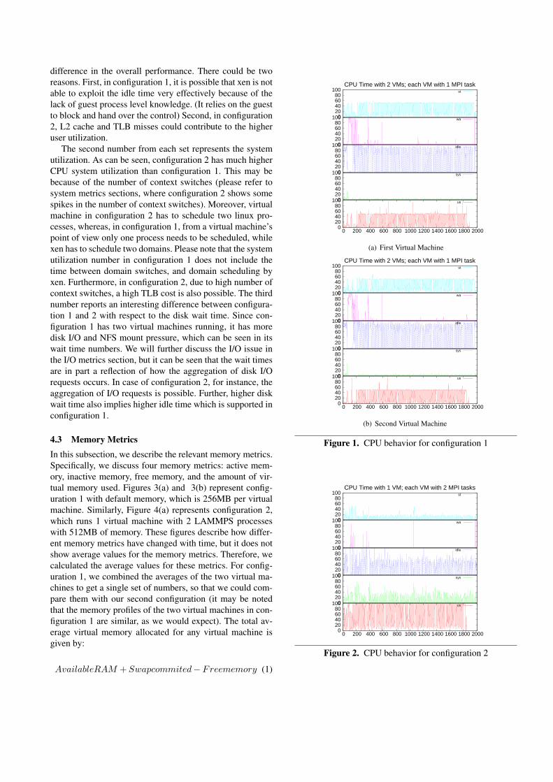
4.2 CPU MetricsIn this subsection, we present statistics on 5 CPU metricsnamely user, system, wait time, idle, and stolen time. Allnumbers for CPU metrics are in percentages. Figures 1(a)and 1(b) represent configuration 1, which runs two virtualmachines per node with 1 application process per VM. Fig-ure 2 represents configuration 2, which runs two applicationprocesses per VM with one VM per node.
The average CPU time distribution percentage numbersfor the virtual configuration 2 across user, system, wa, idle,and stolen time are 63.9%, 9%, 0.7%, 20.4%, 6% respec-tively. Please note that the virtual machine configuration 2runs 2 application processes per VM/per node. The num-bers in the case of configuration 1 are the following: 27.4%,1%, 4.1% , 39.2%, 28.3% for the first VM and 26.4%, 1.2%,4.5% ,39.5%, 28.4% for the second VM. The stolen time foreach vm in each configuration represents the time when thevm wanted to run but was not scheduled. The idle time, onthe other hand, represents the voluntary wait by the vm. Tocompare the cpu metrics of configuration 1 with configura-tion 2, we must combine the cpu metrics of the two virtualmachines in configuration 1. To combine the two set of met-rics for configuration 1, we can use the following argument.First, the user and system time of each vm in configuration1 can simply be added as the numbers represent the realtime (Since the stolen time is removed from the numbers).Thus, the combined user and system time become 53.8%,and 2.2% respectively. We can not add the idle time and I/Owait times as they contain some busy time of other domains.Second, since the busy time of configuration 1 is 56% (user+ system), the idle time is 44% as a whole for configuration1. Third, to get the I/O wait time out of the idle time, wecan use the proportion of the I/O wait time with respect tothe idle time of an individual vm of configuration 1. Thisway the I/O wait time is estimated to be 2.6% for configu-ration 1 and the remaining time, that is 41.4% as idle time.Therefore, the numbers for configuration 1 are 53.8%, 2.2%,2.6%, 41.4% and for configuration 2 are 63.9%, 9%, 0.7%,26.4% (idle + stolen time). Next, we study the cpu metricsindividually for both configurations.
The first number is the CPU user utilization. The cpuuser utilization for configuration 1, which runs two virtualmachines on a physical node with each virtual machinerunning one process, is 53.8%. Similarly, configuration 2reports the number at 63.9%. A quick comparison showsthat from a physical node’s perspective, which holds theCPU, there is significant difference. Yet there is not much
difference in the overall performance. There could be tworeasons. First, in configuration 1, it is possible that xen is notable to exploit the idle time very effectively because of thelack of guest process level knowledge. (It relies on the guestto block and hand over the control) Second, in configuration2, L2 cache and TLB misses could contribute to the higheruser utilization.
The second number from each set represents the systemutilization. As can be seen, configuration 2 has much higherCPU system utilization than configuration 1. This may bebecause of the number of context switches (please refer tosystem metrics sections, where configuration 2 shows somespikes in the number of context switches). Moreover, virtualmachine in configuration 2 has to schedule two linux pro-cesses, whereas, in configuration 1, from a virtual machine’spoint of view only one process needs to be scheduled, whilexen has to schedule two domains. Please note that the systemutilization number in configuration 1 does not include thetime between domain switches, and domain scheduling byxen. Furthermore, in configuration 2, due to high number ofcontext switches, a high TLB cost is also possible. The thirdnumber reports an interesting difference between configura-tion 1 and 2 with respect to the disk wait time. Since con-figuration 1 has two virtual machines running, it has moredisk I/O and NFS mount pressure, which can be seen in itswait time numbers. We will further discuss the I/O issue inthe I/O metrics section, but it can be seen that the wait timesare in part a reflection of how the aggregation of disk I/Orequests occurs. In case of configuration 2, for instance, theaggregation of I/O requests is possible. Further, higher diskwait time also implies higher idle time which is supported inconfiguration 1.
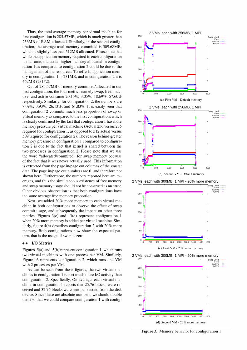
4.3 Memory MetricsIn this subsection, we describe the relevant memory metrics.Specifically, we discuss four memory metrics: active mem-ory, inactive memory, free memory, and the amount of vir-tual memory used. Figures 3(a) and 3(b) represent config-uration 1 with default memory, which is 256MB per virtualmachine. Similarly, Figure 4(a) represents configuration 2,which runs 1 virtual machine with 2 LAMMPS processeswith 512MB of memory. These figures describe how differ-ent memory metrics have changed with time, but it does notshow average values for the memory metrics. Therefore, wecalculated the average values for these metrics. For config-uration 1, we combined the averages of the two virtual ma-chines to get a single set of numbers, so that we could com-pare them with our second configuration (it may be notedthat the memory profiles of the two virtual machines in con-figuration 1 are similar, as we would expect). The total av-erage virtual memory allocated for any virtual machine isgiven by:
AvailableRAM + Swapcommited−Freememory (1)
0 20 40 60 80
100
0 200 400 600 800 1000 1200 1400 1600 1800 2000
us 0 20 40 60 80
100 sys 0 20 40 60 80
100 idle 0 20 40 60 80
100 wa 0 20 40 60 80
100CPU Time with 2 VMs; each VM with 1 MPI task
st
(a) First Virtual Machine
0 20 40 60 80
100
0 200 400 600 800 1000 1200 1400 1600 1800 2000
us 0 20 40 60 80
100 sys 0 20 40 60 80
100 idle 0 20 40 60 80
100 wa 0 20 40 60 80
100CPU Time with 2 VMs; each VM with 1 MPI task
st
(b) Second Virtual Machine
Figure 1. CPU behavior for configuration 1
0 20 40 60 80
100
0 200 400 600 800 1000 1200 1400 1600 1800 2000
us 0 20 40 60 80
100 sys 0 20 40 60 80
100 idle 0 20 40 60 80
100 wa 0 20 40 60 80
100CPU Time with 1 VM; each VM with 2 MPI tasks
st
Figure 2. CPU behavior for configuration 2
Thus, the total average memory per virtual machine forfirst configuration is 285.57MB, which is much greater than256MB of RAM allocated. Similarly, in the second config-uration, the average total memory commited is 509.68MB,which is slightly less than 512MB allocated. Please note thatwhile the application memory required in each configurationis the same, the actual higher memory allocated in configu-ration 1 as compared to configuration 2 could be due to themanagement of the resources. To refresh, application mem-ory in configuration 1 is 231MB, and in configuration 2 it is462MB (231*2).
Out of 285.57MB of memory commited/allocated in ourfirst configuration, the four metrics namely swap, free, inac-tive, and active consume 20.15%, 3.05%, 18.69%, 57.60%respectively. Similarly, for configuration 2, the numbers are8.09%, 3.93%, 26.13%, and 61.83%. It is easily seen thatconfiguration 2 commits much less proportion of swap orvirtual memory as compared to the first configuration, whichis clearly confirmed by the fact that configuration 1 has morememory pressure per virtual machine (Actual 256 versus 285required for configuration 1, as opposed to 512 actual versus509 required for configuration 2). The reason behind greatermemory pressure in configuration 1 compared to configura-tion 2 is due to the fact that kernel is shared between thetwo processes in configuration 2. Please note that we usethe word “allocated/commited” for swap memory becauseof the fact that it was never actually used. This informationis extracted from the page in/page out columns of the vmstatdata. The page in/page out numbers are 0, and therefore notshown here. Furthermore, the numbers reported here are av-erages, and thus the simultaneous existence of free memoryand swap memory usage should not be construed as an error.Other obvious observation is that both configurations havethe same average free memory proportion.
Next, we added 20% more memory to each virtual ma-chine in both configurations to observe the effect of swapcommit usage, and subsequently the impact on other threemetrics. Figures 3(c) and 3(d) represent configuration 1when 20% more memory is added per virtual machine. Sim-ilarly, figure 4(b) describes configuration 2 with 20% morememory. Both configurations now show the expected pat-tern, that is the usage of swap is zero.
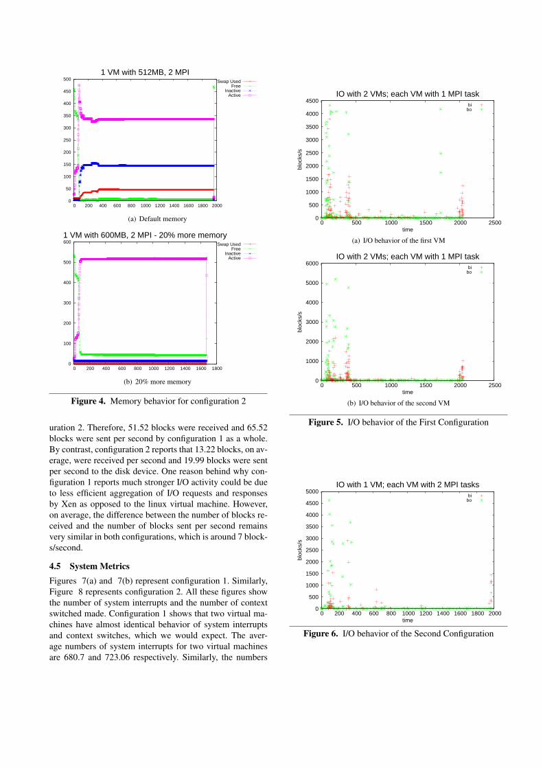
4.4 I/O MetricsFigures 5(a) and 5(b) represent configuration 1, which runstwo virtual machines with one process per VM. Similarly,Figure 6 represents configuration 2, which runs one VMwith 2 processes per VM.
As can be seen from these figures, the two virtual ma-chines in configuration 1 report much more I/O activity thanconfiguration 2. Specifically, On average, each virtual ma-chine in configuration 1 reports that 25.76 blocks were re-ceived and 32.76 blocks were sent per second from the diskdevice. Since these are absolute numbers, we should doublethem so that we could compare configuration 1 with config-
0
50
100
150
200
250
0 500 1000 1500 2000 2500
2 VMs, each with 256MB, 1 MPISwap Used
FreeInactive
Active
(a) First VM - Default memory
0
50
100
150
200
250
0 500 1000 1500 2000 2500
2 VMs, each with 256MB, 1 MPISwap Used
FreeInactive
Active
(b) Second VM - Default memory
0
50
100
150
200
250
300
0 200 400 600 800 1000 1200 1400 1600 1800
2 VMs, each with 300MB, 1 MPI - 20% more memorySwap Used
FreeInactive
Active
(c) First VM - 20% more memory
0
50
100
150
200
250
300
0 200 400 600 800 1000 1200 1400 1600 1800
2 VMs, each with 300MB, 1 MPI - 20% more memorySwap Used
FreeInactive
Active
(d) Second VM - 20% more memory
Figure 3. Memory behavior for configuration 1
0
50
100
150
200
250
300
350
400
450
500
0 200 400 600 800 1000 1200 1400 1600 1800 2000
1 VM with 512MB, 2 MPISwap Used
FreeInactive
Active
(a) Default memory
0
100
200
300
400
500
600
0 200 400 600 800 1000 1200 1400 1600 1800
1 VM with 600MB, 2 MPI - 20% more memorySwap Used
FreeInactive
Active
(b) 20% more memory
Figure 4. Memory behavior for configuration 2
uration 2. Therefore, 51.52 blocks were received and 65.52blocks were sent per second by configuration 1 as a whole.By contrast, configuration 2 reports that 13.22 blocks, on av-erage, were received per second and 19.99 blocks were sentper second to the disk device. One reason behind why con-figuration 1 reports much stronger I/O activity could be dueto less efficient aggregation of I/O requests and responsesby Xen as opposed to the linux virtual machine. However,on average, the difference between the number of blocks re-ceived and the number of blocks sent per second remainsvery similar in both configurations, which is around 7 block-s/second.
4.5 System MetricsFigures 7(a) and 7(b) represent configuration 1. Similarly,Figure 8 represents configuration 2. All these figures showthe number of system interrupts and the number of contextswitched made. Configuration 1 shows that two virtual ma-chines have almost identical behavior of system interruptsand context switches, which we would expect. The aver-age numbers of system interrupts for two virtual machinesare 680.7 and 723.06 respectively. Similarly, the numbers
0
500
1000
1500
2000
2500
3000
3500
4000
4500
0 500 1000 1500 2000 2500
bloc
ks/s
time
IO with 2 VMs; each VM with 1 MPI taskbi
bo
(a) I/O behavior of the first VM
0
1000
2000
3000
4000
5000
6000
0 500 1000 1500 2000 2500
bloc
ks/s
time
IO with 2 VMs; each VM with 1 MPI taskbi
bo
(b) I/O behavior of the second VM
Figure 5. I/O behavior of the First Configuration
0
500
1000
1500
2000
2500
3000
3500
4000
4500
5000
0 200 400 600 800 1000 1200 1400 1600 1800 2000
bloc
ks/s
time
IO with 1 VM; each VM with 2 MPI tasksbi
bo
Figure 6. I/O behavior of the Second Configuration
0
500
1000
1500
2000
2500
3000
3500
4000
4500
0 500 1000 1500 2000 2500
No.
of In
terr
upts
time
system metrics with 2 VMs; 1 MPI/vmintrcs
(a) First VM
0
500
1000
1500
2000
2500
3000
3500
4000
4500
0 500 1000 1500 2000 2500
No.
of In
terr
upts
time
system metrics with 2 VMs; 1 MPI/vmintrcs
(b) Second VM
Figure 7. System Behavior for configuration 1
0
10000
20000
30000
40000
50000
60000
70000
80000
90000
0 200 400 600 800 1000 1200 1400 1600 1800 2000
No.
of In
terr
upts
time
system metrics with 1 VM; 2 MPI/vmintrcs
Figure 8. System Behavior of the Second Configuration
for context switches are 651.14 for first virtual machine and681.7 for the second virtual machine. Therefore, for config-uration 1 as a whole, the average numbers for interrupts andcontext switches are 701.88 and 666.42 per second respec-tively. The average numbers for configuration 2 are 1357.53and 1698.1 per second for interrupts and context switches re-spectively. Interestingly, configuration 2 shows some spikesfor the number of context switches, but the average numberof context switches in configuration 2 remains low. It canbe easily seen that by doubling the average numbers in con-figuration 1, we get close to configuration 2. However, thedoubling exercise clearly shows that while the number of in-terrupts in configuration 1 is more than configuration 2, theopposite is true for context switches.
Further, while the figures show that the average numbersof interrupts and context switches are similar in both con-figurations, they do not follow a particular order. This maybe due to following scenarios: Not every interrupt causesa context switch (such as if the Interrupt Descriptor Table(IDT) entry does not point to a task-gate) and not every con-text switch is associated with an interrupt (such as if a taskyields). Further, it is possible that certain interrupts may havebeen masked and serviced later, or an interrupt may causemultiple context switches. Please also note that, the VMstatis configured to report every 1 second, and therefore, it ispossible that the boundary interrupts and context switchesmay not be aligned.
5. DiscussionIn this section, we try to fit the four metrics (CPU, mem-ory, IO, and system) together into a big picture. First, wecan see that the percentage of CPU user time in configura-tion 2 is much higher than in configuration 1, which sug-gests that configuration 2 is efficient in terms of executingapplication code. Yet, the wall clock times of configuration1 and 2 do not reflect the higher difference between the usercpu utilization. This could be due to the fact that the usercode weight may not be very high as compared to the systemcode weight. Second, although configuration 2 has a higherpercentage of CPU utilization in general, which is seen bythe idle numbers, it also has a higher CPU system utiliza-tion. The higher system utilization in configuration 2 maybe related to the higher cost of context switching, TLB andcache misses. Third, application I/O behavior in configura-tion 1 clearly reflects a far greater activity than configuration2. This is confirmed by the higher disk wait time (wa) per-centage in configuration 1, which is almost 4 times higherthan configuration 2. Higher I/O activity may also explainwhy configuration 1 requires higher memory allocation.
From a flexibility standpoint, configuration 1 offers moreflexibility such as the ability to move virtual machines tospare nodes in the case of faults without disrupting theapplication. This added flexibility of configuration 1 couldbe preferred to configuration 2, even though configuration 1
has more performance penalty than configuration 2. This isthe crux of our study
6. ConclusionIn this paper, we have shown that in terms of wall clocktime, the difference in overall performance is 3%, with con-figuration 2 being more efficient. Yet, the four metrics thatwe have studied reflect different results. CPU usage resultsare interesting in terms of the disk wait, CPU idle num-bers, and user code utilization. Memory allocation/usage isalso dissimilar in two configurations. Further, I/O behav-ior shows a markedly different behavior in one configura-tion with respect to another. Finally, system interrupts andcontext switches are similar on average with few spikes forcontext switches in configuration 2. To sum up, our studyprovides details about the impact of virtualization on HPCapplications such as LAMMPS. The study specifically shedslight on how different virtual configurations impact the over-all performance, and also how the configurations impact theindividual performance metrics. Further the study finds thatthere is some evidence to suggest that a linux virtual ma-chine handles the application and its resources better thanXen does. Moreover, a thematic implication of this study isthat application containers, such as linux virtual machines,could be given more control than hypervisors such as Xen,in handling applications and their resources for efficiencypurposes.
References[1] Padma Apparao, Srihari Makineni, and Don Newell. Charac-
terization of network processing overheads in xen. In VTDC’06: Proceedings of the 2nd International Workshop on Virtu-alization Technology in Distributed Computing, page 2, Wash-ington, DC, USA, 2006. IEEE Computer Society.
[2] Paul Barham, Boris Dragovic, Keir Fraser, Steven Hand, TimHarris, Alex Ho, Rolf Neugebauer, Ian Pratt, and AndrewWarfield. Xen and the art of virtualization. In Proceedingsof the nineteenth ACM symposium on Operating System sPrinciples (SOSP19), pages 164–177. ACM Press, 2003.
[3] D. R. Engler, M. F. Kaashoek, and J. O’Toole, Jr. Exokernel:an operating system architecture for application-level resourcemanagement. In SOSP ’95: Proceedings of the fifteenth ACMsymposium on Operating systems principles, pages 251–266,New York, NY, USA, 1995. ACM.
[4] Michael R. Hines and Kartik Gopalan. Memx: supportinglarge memory workloads in xen virtual machines. In VTDC’07: Proceedings of the 3rd international workshop on Vir-tualization technology in distributed computing, pages 1–8,New York, NY, USA, 2007. ACM.
[5] W. Huang, J. Liu, B. Abali, and D.K. Panda. A Case forHigh Performance Computing with Virtual Machines. In 20thACM International Conference on Supercomputing (ICS ’06)Cairns, Queensland, Australia, June 2006.
[6] Wei Huang, Matthew J. Koop, Qi Gao, and Dhabaleswar K.Panda. Virtual machine aware communication libraries for
high performance computing. In SC ’07: Proceedings of the2007 ACM/IEEE conference on Supercomputing, pages 1–12,New York, NY, USA, 2007. ACM.
[7] Ivan Krsul, Arijit Ganguly, Jian Zhang, Jose A. B. Fortes, andRenato J. Figueiredo. Vmplants: Providing and managingvirtual machine execution environments for grid computing.In SC ’04: Proceedings of the 2004 ACM/IEEE conference onSupercomputing, page 7, Washington, DC, USA, 2004. IEEEComputer Society.
[8] Jiuxing Liu, Wei Huang, Bulent Abali, and Dhabaleswar K.Panda. High performance vmm-bypass i/o in virtual ma-chines. In ATEC ’06: Proceedings of the annual conference onUSENIX ’06 Annual Technical Conference, pages 3–3, Berke-ley, CA, USA, 2006. USENIX Association.
[9] A. Menon, J. R. Santos, Y. Turner, G. Janakiraman, andW. Zwaenepoe. Diagnosing performance overhead in the xenvirtual machine environment. In Proceedings of the 1st ACMConference on Virtual Execution Environments, June 2005.
[10] Arun Babu Nagarajan, Frank Mueller, Christian Engelmann,and Stephen L. Scott. Proactive fault tolerance for HPC withXen virtualization. In ICS ’07: Proceedings of the 21st annualinternational conference on Supercomputing, pages 23–32,New York, NY, USA, 2007. ACM Press.
[11] Dan Pelleg, Muli Ben-Yehuda, Rick Harper, Lisa Spainhower,and Tokunbo Adeshiyan. Vigilant: out-of-band detectionof failures in virtual machines. SIGOPS Oper. Syst. Rev.,42(1):26–31, 2008.
[12] Steve Plimpton. Fast parallel algorithms for short-rangemolecular dynamics. J. Comput. Phys., 117(1):1–19, 1995.
[13] Fernando Rodríguez, Felix Freitag, and Leandro Navarro. Onthe use of intelligent local resource management for improvedvirtualized resource provision: challenges, required features,and an approach. In HPCVirt ’08: Proceedings of the 2ndworkshop on System-level virtualization for high performancecomputing, pages 24–31, New York, NY, USA, 2008. ACM.
[15] Ron Brightwell Suzanne Kelly. Software architecture of thelight weight kernel, catamount. In 47th Cray User Group(CUG 2005), 2005.
[16] Samuel Thibault and Tim Deegan. Improving performanceby embedding hpc applications in lightweight xen domains.In HPCVirt ’08: Proceedings of the 2nd workshop on System-level virtualization for high performance computing, pages 9–15, New York, NY, USA, 2008. ACM.
[17] Jian Wang, Kwame-Lante Wright, and Kartik Gopalan. Xen-loop: a transparent high performance inter-vm network loop-back. In HPDC ’08: Proceedings of the 17th interna-tional symposium on High performance distributed comput-ing, pages 109–118, New York, NY, USA, 2008. ACM.
[18] Lamia Youseff, Rich Wolski, Brent Gorda, and ChandraKrintz. Paravirtualization for HPC Systems. In ISPA Work-shop on XEN in HPC Cluster and Grid Computing Environ-ments (XHPC’06), pages 474–486, December 2006.