39
Performance Engineering Prof. Jerry Breecher Looking at Random Data & A Simulation Example
| Date post: | 29-Dec-2015 |
| Category: |
Documents |
| Upload: | aleesha-manning |
| View: | 220 times |
| Download: | 3 times |

Performance Engineering
Prof. Jerry Breecher
Looking at Random Data &A Simulation Example

Goals:1. Look at the nature of random data. What happens as
random data is used in multiple operations?
2. Look at how network arrivals really work – are arrivals random or do they follow some other pattern?
3. Use our simulation techniques to study these patterns (so this is really an example of simulation usage).
4. Determine the difference in behavior as a result of network arrival patterns.
Random Data
1. Suppose we have a random number generator. And suppose we run a program using that data multiple times.
2. Do the results of those multiple program executions converge or diverge?
3. There is no simple intuitive answer to this question, so let’s try it.
Random Arrivals

Random Data1. Let’s take a very simple piece of code:
if ( random() >= 0.5 ) HeadsGreaterThanTails++;else HeadsGreaterThanTails--;
2. When we run the program, we collect the value of the variable every 100 million iterations – and do it for a total of 1 billion iterations.
3. Here’s a sample run.Iterations Proc 0
100,000,000 -10299
200,000,000 -4245
300,000,000 5141
400,000,000 3197
500,000,000 -1313
600,000,000 -25941
700,000,000 -24093
800,000,000 -24661
900,000,000 -27123
1,000,000,000 -23997
After 400 million iterations, there were 3192 more “heads” than “tails”.

Random Data1. Now lets do that same thing for 8 processes2. What do you think will happen to the numbers?
– Will some process always have more heads than tails?– Will the difference between results for processes depend on how many
iterations have been done?
3. Here’s the result for 8 processes:
Iterations Proc 0 Proc 1 Proc 2 Proc 3 Proc 4 Proc 5 Proc 6 Proc 7
100,000,000 -10299 -9319 -1063 6743 8633 -4421 8123 -1367
200,000,000 -4245 -10227 3657 -23059 24885 -26655 25865 -5871
300,000,000 5141 -6819 255 -20175 14469 -33389 27077 -7299
400,000,000 3197 -8155 -5379 -6633 27387 -50509 24531 2339
500,000,000 -1313 -10547 -153 -14679 29335 -51963 23097 -3705
600,000,000 -25941 -29847 -26371 5027 32857 -49505 27089 -1659
700,000,000 -24093 -26331 -43401 13153 24471 -26899 4561 -47
800,000,000 -24661 -35315 -31233 41 20425 -11861 13837 -4217
900,000,000 -27123 -33049 -44461 -11769 -3283 -12477 15865 -2107
1,000,000,000 -23997 -15483 -44535 22889 -8447 -13671 15743 6023

Random DataAnd here’s the graph for those 8 processes – note there’s been a
constant amount added to each value to get all the outputs positive.
Random Patterns For 8 Processes
0
10000
20000
30000
40000
50000
60000
70000
80000
90000
100000
0 200,000,000 400,000,000 600,000,000 800,000,000 1,000,000,000 1,200,000,000
Iterations (Units of 100Million)
(Hea
ds
- T
ails
) +
60,
000 Proc 0
Proc 1
Proc 2
Proc 3
Proc 4
Proc 5
Proc 6
Proc 7

Random DataAs you can see in the last graph, the statistics are terrible – it’s hard to
determine the pattern for multiple runs.So the program was run 10,000 times. And the minimum and maximum
count was taken at each time interval for those 10,000 runs.
The Max and Min values in All Runs
0
50000
100000
150000
200000
250000
0 200000000 400000000 600000000 800000000 1000000000 1200000000
Iterations
Max
/Min
+ 1
2500
0
Min of all runs
Max of all runs

Random DataBut, what happens if the processes doing random events interact with each
other?
This is the case if the programs are all accessing the same disk – we randomly choose which block in a large file is being written to. But each process must compete for the file lock and for disk access.
Here’s the behavior of 10 disk-writing processes for 10,000 seconds. The numbers represent disk writes for that process during the time interval.
Secs Proc 0 Proc 1 Proc 2 Proc 3 Proc 4 Proc 5 Proc 6 Proc 7 Proc 8 Proc 9
1000 21660 21650 21810 21800 21790 21720 21850 21740 21640 21730
2000 43000 42960 43080 43120 43220 42960 43190 43110 42900 43080
3000 64790 64650 64850 64930 65060 64680 64900 64860 64770 64940
4000 86610 86450 86620 86680 86750 86530 86640 86660 86560 86690
5000 108450 108280 108370 108450 108520 108410 108480 108380 108400 108580
6000 130010 129860 129990 129950 129980 130050 130090 130010 129910 130080
7000 151730 151600 151710 151730 151730 151770 151750 151820 151750 151800
8000 173340 173340 173400 173640 173480 173400 173520 173660 173470 173500
9000 194950 195050 195010 195300 195090 195000 195230 195440 195130 195150
10000 216760 216880 216780 217140 216860 216740 216990 217240 216880 216960
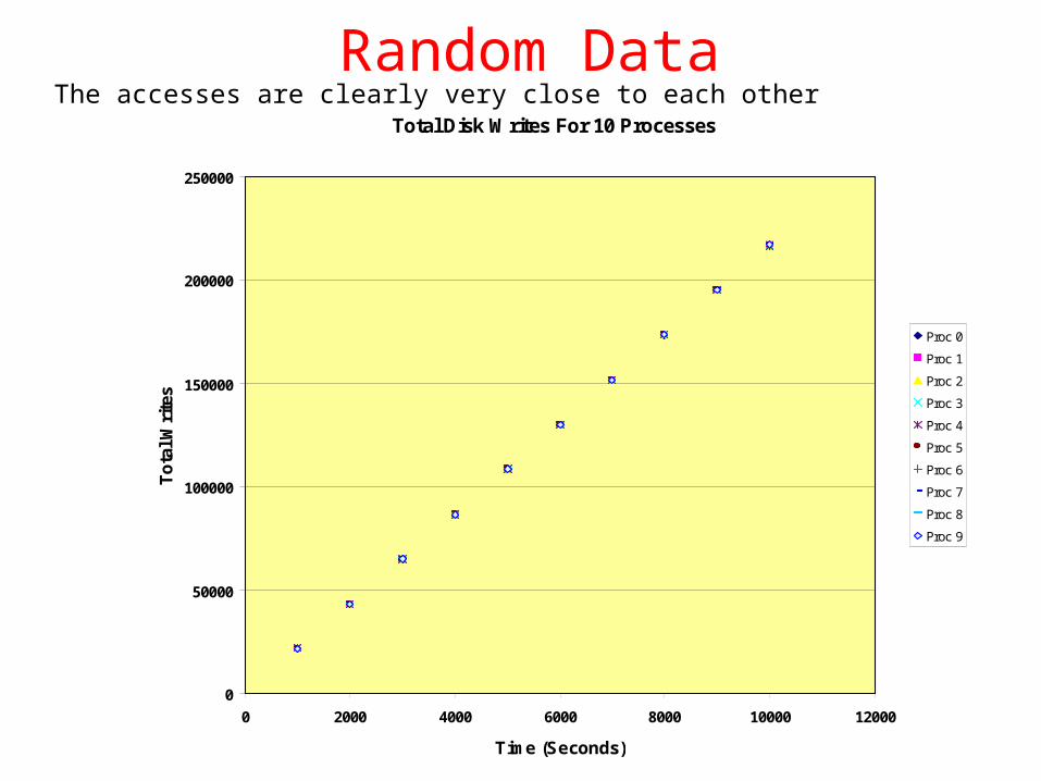
Random DataThe accesses are clearly very close to each other
Total Disk Writes For 10 Processes
0
50000
100000
150000
200000
250000
0 2000 4000 6000 8000 10000 12000
Time (Seconds)
To
tal W
rite
s
Proc 0
Proc 1
Proc 2
Proc 3
Proc 4
Proc 5
Proc 6
Proc 7
Proc 8
Proc 9

Random DataComparing the 10 processes. This is the spread (difference) of the maximum
less the minimum accesses for the process.
Disk Access Rates With Time - It is (Max Access - Min Access)
0
100
200
300
400
500
600
0 2000 4000 6000 8000 10000 12000
Time (Seconds)
Dif
fere
nce
In A
cces
ses

Random DataComparing the 10 processes. Here’s how their relative performance varies over
time. Note that no one process is always the minimum or the maximum performer.
Process Writes - How they deviate from the minimum value
0
100
200
300
400
500
600
0 1000 2000 3000 4000 5000 6000 7000 8000 9000 10000
Time (Seconds)
Pro
cess
Wri
tes
com
par
ed t
o m
inim
um
pro
cess
Proc 0
Proc 1
Proc 2
Proc 3
Proc 4
Proc 5
Proc 6
Proc 7
Proc 8
Proc 9

Another Numerical Example
I have two virtual cats, who share a single can of food at each meal. My cats are very finicky and get angry if their portions are unequal. I am finicky too, and I don't like dirtying dishes when I divvy it up.
To split the food, then, I upend the open can of food onto a flat plate, then carefully lift the can off, leaving a perfectly formed virtual cylinder of food.
Then I use the vanishingly small circular edge of the can to carefully cut the food into two exactly equal portions, one of which is shaped like a crescent moon, the other a cat's eye, or mandorla.

Another Numerical Example
X
X
AA
B B

Another Numerical Example// //////////////////////////////////////////////////////////////////////// We're trying to solve the following problem.// Given two circles, how close should the centers of the circles be such// that the area subtended by the arcs of the two circles is exactly one// half the total area of the circle.//// See example 2.3.8 in Leemis & Park.// We use the book's definition for Uniform - see 2.3.3// Here's how this works. Try a number of different distances between // the two circle centers. Then for the ones that are most successful,// zoom in to do them in more detail.// //////////////////////////////////////////////////////////////////////#include <math.h>#include <stdlib.h>#define PI 3.1415927#define TRUE 1#define FALSE 0
// Prototypesdouble GetRandomNumber( void );void InitializeRandomNumber( );double ModelTwoCircles( double, int );double Uniform( double min, double max) { return( min + (max - min)*GetRandomNumber() );}

int main( int argc, char *argv[] ) { double Distance, Result = 0; double FirstSample = 0.1, LastSample = 1.9; double Increment, NewFirstSample; double BestDistance; int NumberOfSamples = 5000; int AnswerIsFound = FALSE;
InitializeRandomNumber(); while ( !AnswerIsFound ) { printf( "\nNext Iteration starts at %f\n", FirstSample ); Increment = (LastSample - FirstSample)/10; NumberOfSamples = 2 * NumberOfSamples; for ( Distance = FirstSample; Distance <= LastSample; Distance += Increment ){ Result = ModelTwoCircles( Distance, NumberOfSamples ); if ( Result - 0.5000 > 0 ) NewFirstSample = Distance; if ( (0.5 - Result) < 0.0001 && (Result - 0.5) < 0.0001 ) { AnswerIsFound = TRUE; BestDistance = Distance; } printf( "Distance = %8.6f, Fraction = %8.6f\n", Distance, Result ); } FirstSample = NewFirstSample - 2 * Increment; LastSample = FirstSample + 4 * Increment; } printf( "\nThe best Distance is at %f using %d samples\n",
BestDistance, NumberOfSamples );}

double ModelTwoCircles( double Distance, int NumberOfSamples ) { double HitsInOneCircle = 0, HitsInTwoCircles = 0; double x, y, SecondDistance; int Samples; for ( Samples = 0; Samples < NumberOfSamples; Samples++ ) { do { x = Uniform( -1, 1 ); y = Uniform( -1, 1 ); } while ( (x * x) + (y * y) >= 1 ); // Loop until value in circle HitsInOneCircle++; SecondDistance = sqrt( ( x - Distance ) * (x - Distance ) + (y * y) ); if ( SecondDistance < 1.0 ) { HitsInTwoCircles++; // printf( "Samples: Second Distance = %8.6f\n", SecondDistance ); } } // End of for return( HitsInTwoCircles / HitsInOneCircle );}

Network Arrivals
1. In our queueing analysis, we’ve assumed random arrivals (Poisson distribution, with exponentially distributed inter-arrival times.)
2. This leads to our analysis of M/M/1 queues with – Utilization = Service Time/Arrival Time and with – Queue Length = U / ( 1 – U ).
3. We generated uniformly distributed random numbers and based on those were able to derive the exponential arrival times and Poisson distributions.
But is this how networks behave?
Random Arrivals

Network Arrivals
On the Self-Similar Nature of Ethernet TrafficLeland, Taqqu, Willinger, Wilson. IEEE/ACM ToN, Vol. 2, pp 1-15, 1994
1. Establish self-similar nature of Ethernet traffic
2. Illustrate the differences between self-similar and standard models
3. Show serious implications of self-similar traffic for design, control and performance analysis of packet-based communication systems
Self-Similar Arrivals
This how networks really behave?

What Did Leland et. al Measure?Millions of packets from many workstations, as recorded on Bellcore internal networks.
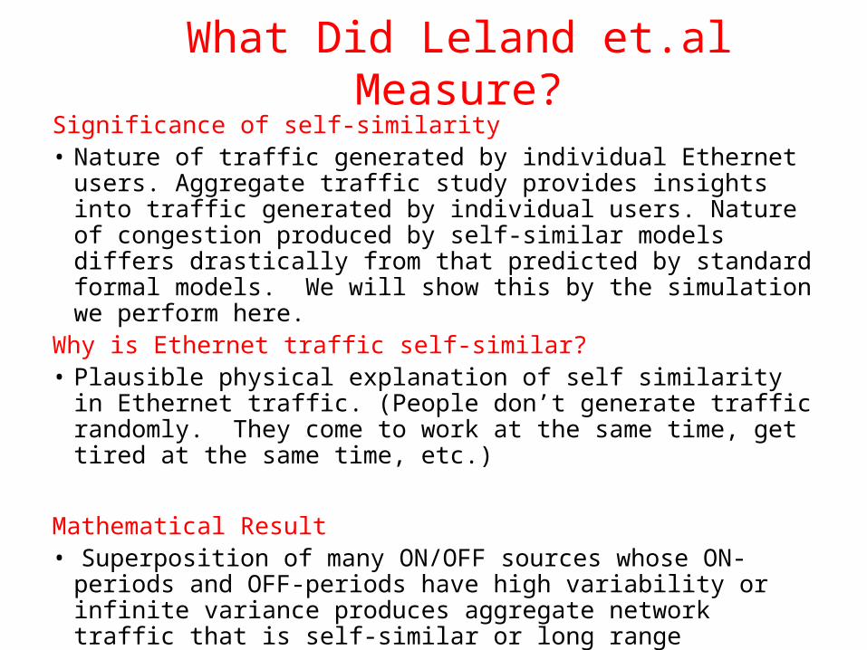
What Did Leland et.al Measure?Significance of self-similarity• Nature of traffic generated by individual Ethernet users. Aggregate
traffic study provides insights into traffic generated by individual users. Nature of congestion produced by self-similar models differs drastically from that predicted by standard formal models. We will show this by the simulation we perform here.
Why is Ethernet traffic self-similar?• Plausible physical explanation of self similarity in Ethernet traffic.
(People don’t generate traffic randomly. They come to work at the same time, get tired at the same time, etc.)
Mathematical Result• Superposition of many ON/OFF sources whose ON-periods and OFF-
periods have high variability or infinite variance produces aggregate network traffic that is self-similar or long range independent.
(Infinite variance here means that there are some samples with a very long inter-arrival time (lunch hour is a very long time!)

What Did Leland et.al Measure?
So are these bursts “random”? Can you tell by looking at the data.
The answer is the data is bunched together – it’s not spread uniformly – and to be self-similar, the “bunches” themselves form “super-bunches”.
Where does “Self-Similar” Data Occur?It occurs throughout nature. Also called Pareto Distribution,
Bradford, Zipf, and various other names.
• Distribution of books checked out of a library.• Distribution of lengths of rivers in the world.
It’s NOT the same as an exponential distribution! (But it can look fairly close.)
Fractals are an example of self-similarity.

Exponential and Self-Similar DataExponential Cumulative Function F(x) = 1 – e(-ax)
Exponential Probability Density Function (PDF) f(x) = a e(-ax)
Pareto Cumulative Function F(x) = 1 – (X0 / (X0 + x) )b
Pareto Probability Density Function (PDF) f(x) = b X0 b
/ (X0+x) (b+1)
In these equations:a = 1 (exponent falls to 1/e when x = 1.) The mean of these values is 1. Turns out the variance is also 1. The exponent is special that way.
X0 is = 2. Then b was adjusted so that it gave a mean of 1.
Arrivals for both distributions therefore have the same mean value.
Theoretical: Exponential + Pareto
0
0.2
0.4
0.6
0.8
1
1.2
1.4
1.6
0 1 2 3 4 5 6 7 8
X
PD
F +
Cu
m
Exponential Cumulative
Pareto. Cumulative(yellow)
Pareto PDF
Exp. PDF (purple)

Exponential and Self-Similar DataTheoretical: Exponential + Pareto
0
0.2
0.4
0.6
0.8
1
1.2
1.4
1.6
0 1 2 3 4 5 6 7 8
X
PD
F +
Cu
m
Exponential Cumulative
Pareto. Cumulative(yellow)
Pareto PDF
Exp. PDF (purple)
Theoretical: Exponential & Pareto
0
0.002
0.004
0.006
0.008
0.01
0.012
5 6 7
X
PD
F
Exp PDF (Black)
Pareto PDF (Purple)Note that the Pareto data has a higher value at the limits – this is what leads to it being self-same and to the data having a large variance.

Simulation Example 25
Simulation So I wrote a simulator.
There are two parts I especially want to show you:
1. The “guts” of the simulator – how events are taken off a queue and are processed; that processing generates new events.
2. How data is generated – starting with a random number in the range 0 1, how do we get an exponential distribution.
• Here’s the code I used for the simulation. It’s not beautiful, but the price is right.
http://www.cs.wpi.edu/~jb/CS533/Lectures/ArrivalSimulation.c

Simulation Example 26
Simulation SCHEMATIC OF EVENT DRIVEN SIMULATION
OF A NETWORK
Initialize
Determine Next Event
Set current time to the time of this event.
Packet approaches network
Event Queue
Is it arrival or completion?
Put packet on network; if queue WAS empty, generate a completion event
Network Service Completed
Take packet off queue; if queue still has a packet, then generate completion.
Update Statistics
Determine when next packet will finish.Determine future time for next packet
arriving.
Generate event for “Packet arrives at Q" Generate event for “Service Completed"
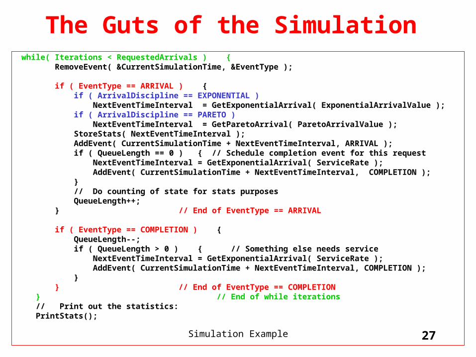
Simulation Example 27
The Guts of the Simulation while( Iterations < RequestedArrivals ) { RemoveEvent( &CurrentSimulationTime, &EventType ); if ( EventType == ARRIVAL ) { if ( ArrivalDiscipline == EXPONENTIAL ) NextEventTimeInterval = GetExponentialArrival( ExponentialArrivalValue ); if ( ArrivalDiscipline == PARETO ) NextEventTimeInterval = GetParetoArrival( ParetoArrivalValue ); StoreStats( NextEventTimeInterval ); AddEvent( CurrentSimulationTime + NextEventTimeInterval, ARRIVAL ); if ( QueueLength == 0 ) { // Schedule completion event for this request NextEventTimeInterval = GetExponentialArrival( ServiceRate ); AddEvent( CurrentSimulationTime + NextEventTimeInterval, COMPLETION ); } // Do counting of state for stats purposes QueueLength++; } // End of EventType == ARRIVAL
if ( EventType == COMPLETION ) { QueueLength--; if ( QueueLength > 0 ) { // Something else needs service NextEventTimeInterval = GetExponentialArrival( ServiceRate ); AddEvent( CurrentSimulationTime + NextEventTimeInterval, COMPLETION ); } } // End of EventType == COMPLETION } // End of while iterations // Print out the statistics: PrintStats();

Simulation Example 28
Data Generation Here’s the question we want to answer – given a PDF, how do we find what value generates a particular value of that PDF.
For instance, applying this question to the Exponential Probability Density Function (PDF) f(x) = a e(-ax) , or
f(x) = e –x for a == 1.
what value of x produces the resultant f(x)? We generate random numbers in the range of 0 1. These are the f(x). So what values of x will give us this range of f(x)?
For x = 0, f(x) == 1; For x = infinity, f(x) = 0.
This inverse mapping is most easily accomplished by taking the inverse function. x = -ln( f(x) ) x = -ln( rand() )
Here’s the essence of this code:
double GetExponentialArrival( double Argument ) { return( -log( 1.0 - GetRandomNumber() )/ Argument );} // End of GetExponentialArrival

Simulation Example 29
Data Generation So having an inverse function is very nice – it’s one reason that using
exponential function is so handy, and so universal. But for the Pareto PDF
f(x) = b X0b / (X0+x)(b+1)
The inverse function is much more difficult to find in this case. I solved this by doing a search. The binary search algorithm goes like this:
1. Pick a random number in the range 0 1; R = random();2. Calculate an f(y), and f(z) such that one of these is larger than R and
one is smaller than R.3. Calculate f( (y + z )/2 ) – for a value half way between y and z.4. Determine y and z such that f(y) and f(z) again straddle R.5. Loop to Step 3 until the value of ( R – f(y) ) is arbitrarily small.
All this is messy and compute intensive – but that’s the way it is when there’s no inverse function.

Simulation Example 30
Simulation ResultsSimulation Results
0
0.2
0.4
0.6
0.8
1
1.2
1.4
0 2 4 6 8 10
Range
Nu
mb
er I
n r
an
ge
Exponential PDF
Pareto PDF
Results look very similar to the analytical functions.
Simulation Example 31
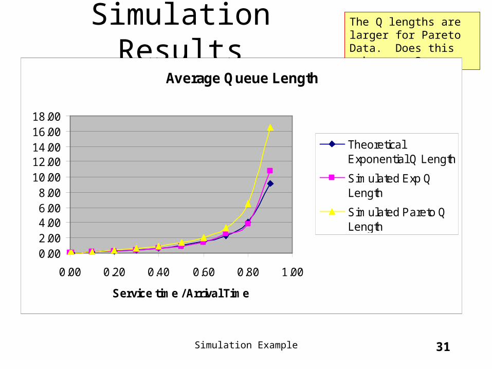
Simulation ResultsThe Q lengths are larger for Pareto Data. Does this make sense?
Average Queue Length
0.002.004.006.008.00
10.0012.0014.0016.0018.00
0.00 0.20 0.40 0.60 0.80 1.00
Service time / Arrival Time
TheoreticalExponential Q Length
Simulated Exp QLength
Simulated Pareto QLength

Simulation Example 32
GraphsThe Utilization is larger for Pareto Data. Does this make sense?
Utilization
0.00
0.20
0.40
0.60
0.80
1.00
0.00 0.20 0.40 0.60 0.80 1.00
Service Time/Arrival time
TheoreticalExponential Utilization
Simulated ExpUtilization
Simulated ParetoUtilization

Simulation Example 33
Marriage & Divorce SimulationThe goal of this exercise to show the simulation of a “society”. In the larger context, it’s an
example of how students might perform a simulation.
Given a body of data, how do we arrange that data in order to represent how the society is behaving. This is essentially a “model” using the data.
There are three ways we go about putting numerical values on this model.:
1. Given a series of equations, can we simply solve the equations?
2. If the equations don’t have a closed form solution, can we solve them recursively. There are no statistics involved here, but all we do is solve each equation over and over again and hope that it converges. This method gives us no details about the population since we’re simply solving equations.
3. We can try for a “real” simulation. In this case, we use the probabilities and a random generator to try to simulate good years and bad years. This allows us to answer much more complex situations. We could now track characteristics for each individual in our society. We could, possibly, see how long a person in our society stays married for instance.

Simulation Example 34
Marriage & Divorce SimulationThere’s lots of stuff on the web, confusing and maybe contradictory:All data is for the US.
In 2007, there were 2,200,000 marriages. This represents a rate of 7.5 per 1000 total population. Note this is 2.2M / 296M = 7.5. (Total US population is higher but some states don’t report.)Another metric which may be saying the same thing is that there are 39.9 marriages per 1000 single women. We’re going to use the first number here.
In 2007, there were 856,000 divorces. This is 3.6 per 1000 total population.
Interesting numbers, but not used here:41% of 1st marriages end in divorce.60% of 2nd marriages end in divorce.74% of 3rd marriages end in divorce.The average remarriage occurs 3.3 years after a divorce.
In 2007 there were 2.400,000 deaths representing a rate of 8.2 per 1000. Details of this on next page.
60% of all marriages last until 1 partner dies
Birth rate is 13.8 per 1,000 population
Recent statistics say that 51% of the adult population is married. This is important because we don’t use it directly as one of our equations – we use it to test if our model gives approximately this answer.

Simulation Example 35
Marriage & Divorce SimulationIn 2007 there were 2.400,000 deaths representing a rate of 8.2 per thousand.
Details on this mortality data are for men and women 65+ :
Death rate for married man is defined as 1.00
Death rate for a widowed man is 1.06 times that of a married man.
Death rate for a divorced or separated man is 1.14 times that of a married man.
Death rate for a never-married man is 1.05 times that of a married man.
Death rate for married woman is defined as 1.00
Death rate for widowed woman is defined as 1.15
Death rate for divorced or separated woman is defined as 1.26
Death rate for a never-married woman is 1.18 times that of a married woman.
This information is from “US Mortality by Economic, Demographic, and Social Characteristics: The National Longitudinal Mortality Study”, Sorlie, Backlund, and Keller, 1995
We use a rate that’s above and below the 8.2 per 1000 for the national average to take into account single and married rates.
DeathMarriedRate = 7.6 per 1000
DeathSingleRate = 8.7 per 1000

Simulation Example 36
Zombie
Single
Married
Reincarnation = 100%
Death while Married
Death while Single
Birth Rate
Marriage RateDivorce RateWidowed
Marriage & Divorce Simulation

Simulation Example 37
Leaving Zombie: Z = - Rbirth * ( S + M )Entering Zombie: Z = + Rdeath-single * S + Rdeath-married * MLeaving Single:S = -2 * Rmarriage * ( S + M ) - Rdeath-single * S Entering Single:S = + Rbirth * ( S + M ) + 2 * Rdivorce * ( S + M ) + Rdeath-married * MLeaving Married:M= -2 * Rdivorce * ( S + M ) - Rdeath-married * MEntering Married:M= + 2 * Rmarriage * ( S + M )
In Steady State – leaving equals entering+ Rdeath-single * S + Rdeath-married * M - Rbirth * ( S + M ) = 0+ Rbirth * ( S + M ) + 2 * Rdivorce * ( S + M ) + Rdeath-married * M -2 * Rmarriage * ( S + M ) - Rdeath-single * S = 0+ 2 * Rmarriage * ( S + M ) - 2 * Rdivorce * ( S + M ) - Rdeath-married * M = 0
Marriage & Divorce Simulation

Simulation Example 38
In Steady State – leaving equals entering
+ Rdeath-single * S + Rdeath-married * M - Rbirth * ( S + M ) = 0
+ Rbirth * ( S + M ) + 2 * Rdivorce * ( S + M ) + Rdeath-married * M -2 * Rmarriage * ( S + M ) - Rdeath-single * S = 0
+ 2 * Rmarriage * ( S + M ) - 2 * Rdivorce * ( S + M ) - Rdeath-married * M = 0
Rearranging these equations gives:
- Rbirth * ( S + M ) + Rdeath-single * S + Rdeath-married * M = 0
+ Rbirth * ( S + M ) - 2 * Rmarriage * ( S + M ) + 2 * Rdivorce * ( S + M ) - Rdeath-single * S + Rdeath-married * M = 0
+ 2 * Rmarriage * ( S + M ) - 2 * Rdivorce * ( S + M ) - Rdeath-married * M = 0
Maybe there’s a solution, but they seem redundant to me.
Marriage & Divorce Simulation
Here are links to the code and executables for this simulation:
MarriageAndDivorceSimulation1.c // Recursively solves the equationsMarriageAndDivorceSimulation1.exe
MarriageAndDivorceSimulation2.c // Does a statistical simulationMarriageAndDivorceSimulation2.exe
MarriageAndDivorceSimulation1.c
Simulation Example 39
WRAPUP
This section has shown the result of a simulation. It’s gone through the coding, the data generation, and the interpretation of results.
If network arrivals are Self-Similar, what about all kinds of other data generated by computers? What about requests arriving at a disk? What about processes arriving at a ready queue?
Is there any computer data that REALLY is random, or is it all self-similar?


