energies

Article

Performance Improvement of a HydraulicActive/Passive Heave Compensation Winch UsingSemi Secondary Motor Control: Experimental andNumerical Verification

Geir-Arne Moslått 1,*, Michael Rygaard Hansen 2 and Damiano Padovani 2

1 Department of Lifting and Handling, National Oilwell Varco, 4639 Kristiansand, Norway2 Department of Engineering Sciences, University of Agder, 4879 Grimstad, Norway; michael.r.hansen@uia.no

(M.R.H.); damiano.padovani@uia.no (D.P.)* Correspondence: geir-arne.moslaatt@nov.com

Received: 28 April 2020; Accepted: 18 May 2020; Published: 25 May 2020�����������������

Abstract: In this paper, a newly developed controller for active heave compensated offshore cranes iscompared with state-of-the-art control methods. The comparison is divided into a numerical parton stability margins as well as operational windows and an experimental validation of the expectedperformance improvement based on a full-scale testing on site with a crane rated to 250 metrictons. Such a crane represents the typical target for the new control method using a combinationof active and passive hydraulic actuation on the main winch. The active hydraulic actuation isa hydrostatic transmission with variable-displacement pumps and variable-displacement motors.The new controller employs feedforward control of the motors’ displacement so that the window ofoperation is increased and, simultaneously, oscillations in the system are markedly reduced.

Keywords: active heave compensation; winch; hydrostatic transmission

1. Introduction

There are high demands for motion compensated offshore cranes today, mostly related to oil andgas, but also the offshore wind industry. The purpose of motion compensation is to decouple the vesselmotion from the connected payload. There are two main categories of compensation. The first is afull 3D compensation (horizontal and vertical plane), while the second is a 1D compensation (verticalplane alone). The most common solution is equipping the crane with a 1D compensation system, andthe vessel with a dynamic positioning system keeps the position in the horizontal plane. This approachworks very well for most subsea operations since the payload motion in the horizontal plane due tothe vessel’s roll, pitch, and yaw becomes insignificant by the dampening effect when the payload isbelow the sea surface. If 1D or 3D compensation is used, the most common methods for the verticalcompensation of the motion are controlling the wire speed in the winch or using a passive motioncompensator mounted directly on the crane’s hook. The wire’s speed control can be done with thedrum directly or with a dedicated cylinder [1]. When the system is drum controlled, it is usually donewith a hydraulic transmission that can be categorized into five types [1–4]:

1. Primary controlled systems with variable-displacement pumps and fixed-displacement motors(VPFM) operated in the closed-circuit configuration.

2. Primary controlled systems with variable-displacement pumps and variable-displacement motors(VPVM) operated in the closed-circuit configuration.

3. Secondary control with a VPVM system operated in closed-circuit configuration with an in-lineaccumulator ensuring constant pressure.

Energies 2020, 13, 2671; doi:10.3390/en13102671 www.mdpi.com/journal/energies

Energies 2020, 13, 2671 2 of 20

4. Active/passive hydraulic systems (also known as “hybrid”) with two VPVM systems where oneof them is secondary controlled, and the other one is primary controlled.

5. Open-circuit systems with a power supply and a pressure-compensated proportional valve.

The active/passive systems dominate the market when looking at crane sizes with lifting capacityabove 100 tons. Pure secondary controlled systems are also an option and could be equipped withboth analog or digital displacement motors. Although digital displacement motors are not a maturesolution at the moment [5], these systems are well suited for the recuperation of energy when subjectedto negative loads [3,6,7]. The secondary control units benefit from higher speed capabilities, andimproved system response compared to the classic primary pump-controlled systems. Secondarycontrol was introduced in 1977 [8] for hydraulic systems but has still not obtained widespread usein the offshore crane market. The main disadvantage is the demand for expensive componentssuch as over-center hydraulic motors or digital displacement hydraulic motors. The active/passivesystem is chosen for further investigation in this paper due to its widespread use. Specifically,the active circuit has untapped improvement potential [9]. In the active part of an active/passivesystem, the motors are equipped with an adjustable displacement. However, the most common activeheave compensation strategy is to utilize the motors as if they were fixed-displacement units (like aVPFM system). This approach results in the pumps used as the control element, while the motors’displacement is not adjusted continuously but simply set to fixed values based on the number of wirelayers on the drum. When VPFM systems are used in active heave compensation (AHC), the maximumexploitable speed for the winch is limited because the fixed-displacement motors are set based on thehigh-torque scenarios. As a result, systems that use this classic control method often have differentmodes to cover a greater speed range. Typically, different modes comprise a normal-speed mode thatallows full load capacity, and a high-speed mode. The high-speed mode operates with reduced motors’displacement; therefore, the winch gets a lower allowable safe working load (SWL).

Linear control approaches for hydrostatic transmission (HST) systems, like classic PID controllers,are still commonly used in industrial applications. However, the HST is a nonlinear system, andresearchers have tried to address this for several years. One of these strategies utilizes nonlinearbackstepping methods [10,11]. Others strategies introduce adaptive control techniques [12–17],or model-based control [18–22]. Some attempts directly towards active heave compensated systemshave also been investigated, like fuzzy PI or PID controller [23,24], position controller with tensionfeedback [25,26], and cascade controllers [27]. To control the winch-drives, one should consider theuse of fault-tolerant control (FTC) approaches [12,28]. There are two main categories of FTC [29],namely, active and passive. The cranes from National Oilvell Varco are, in principle, equipped withparts from both, but should, in general, be seen as a system equipped with passive FTC. The AHCcontroller is a robust linear controller, which is a type of passive FTC. However, the cranes couldalso be equipped with systems that detect critical errors, such as sensor faults or power loss. In theevent of a power failure, the crane uses parameter reconfiguration in the controller, which is a typeof active FTC. E.g., if one of the three hydraulic power units shuts down, the fault is detected,the unit gets isolated, and the control parameters are reconfigured (the process is done on-the-flywithout stopping the AHC operation). Further, it has been some interest regarding the vessel’s motionprediction [30,31] that can be used to improve the controller performance or to predict future events.However, all the aforementioned research is concerned with system performance optimization byexclusively focusing on either the primary control unit or the secondary control unit. In [32] such adual approach was introduced, and it was shown that optimized control of the pumps’ and motors’displacement could yield a better trade-off between response speed and efficiency. The results were,however, not experimentally verified. Another strategy to improve the performance of an HST systemfor an AHC winch system was introduced in [9]. It highlighted that the dynamical properties of thewinch system are highly affected by the motors’ displacement, and maximizing them at low speedwould result in significant improvements in pressure-peaks and control error. The proposed controlstrategy actively adjusts the motors’ displacement and, at the same time, keep the classic primary

Energies 2020, 13, 2671 3 of 20

pump-controller. Thus, the system is a mix of secondary control and primary control and called semisecondary control (SSC). Since the displacement in SSC is active and also load sensitive, the needfor two or more operational modes is removed as well as the corresponding limitations on the SWL.The results from simulations showed increased performance with regards to the maximum winchvelocity and permitted load. It also improved the dynamic response of the winch, which resulted in asmaller control error and smoother winch motion.

Even though the SSC system has been introduced, no systematic evaluation of the new systemhas been put forward, and no full-scale experimental verification of the improved performance hasbeen presented. Both these aspects are, therefore, addressed in this paper. A description of thehydraulic and mechanical winch system is given in the next section, together with a portrayal ofthe new controller. In the third section, the new controller’s effect on stability is reviewed. Then,in section four, a comparison of the classic control method and the new SSC approach are compared ina simulation model. Section five continues with more comparisons that originated from field tests,followed by the conclusions in section six.

2. Control Algorithm and System Description

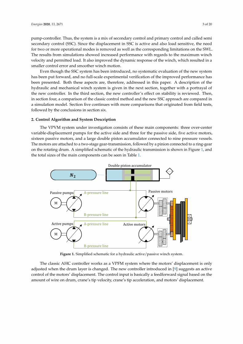
The VPVM system under investigation consists of these main components: three over-centervariable-displacement pumps for the active side and three for the passive side, five active motors,sixteen passive motors, and a large double piston accumulator connected to nine pressure vessels.The motors are attached to a two-stage gear-transmission, followed by a pinion connected to a ring-gearon the rotating drum. A simplified schematic of the hydraulic transmission is shown in Figure 1, andthe total sizes of the main components can be seen in Table 1.

Passive pumps Passive motors

𝑵𝟐

Active pumps Active motors

Double piston accumulator

M

M

A-pressure line

B-pressure line

A-pressure line

B-pressure line

fig_simpleActPasSchematic

Figure 1. Simplified schematic for a hydraulic active/passive winch system.

The classic AHC controller works as a VPFM system where the motors’ displacement is onlyadjusted when the drum layer is changed. The new controller introduced in [9] suggests an activecontrol of the motors’ displacement. The control input is basically a feedforward signal based on theamount of wire on drum, crane’s tip velocity, crane’s tip acceleration, and motors’ displacement.

Energies 2020, 13, 2671 4 of 20

Table 1. Main component data.

Description Total Size

Active motors 1075 cm3/revPassive motors 3440 cm3/revActive pumps 1355 cm3/revPassive pumps 1210 cm3/revGearbox ratio 35.4

Pinion ring-gear ratio 14.17Drum diameter (without wire) 2.8 m

Drum width 1.9 mWire diameter 96 mm

The control structure is depicted in Figure 2, where the parts marked in red represent changesfrom the classical PVFM controller.

𝛼𝑚

𝛼𝑝

Crane kinematics

Vesselmotion

Reference winchposition

Crane pos.

Crane tip vel.

𝐺𝑠𝑦𝑠𝑡𝑒𝑚(𝑠)

Active pump displacement

prediction

Active motor displ., 𝛼𝑚

𝐺𝑝𝑢𝑚𝑝 (𝑠)+ +

Winch pos.

𝐺𝑚𝑜𝑡𝑜𝑟 (𝑠)Active motor displacement computation

Winch pos.

Load cell

fig_newControllerScematic2

Winch pos.Crane tip acc.

Crane tip pos.

−1

−1 𝐾𝑝

𝑢𝑓𝑓

𝑢𝑚

Figure 2. The new control structure.

The classic system’s control uses a conservative fixed value of the motors’ displacement to beable to cope with the required operation, winch stiction, and winch acceleration. The resulting torquepeaks when the winch is switching direction (i.e., scenarios with low speed and high acceleration).The new controller is expected to improve the performance compared to the classical controller. One ofthe main reasons is that the motors are set to maximum displacement whenever the winch is passingzero velocity. This decision will ensure a higher system stiffness and high torque capacity. As a result,lower amplification of the system resonance and smaller pressure peaks are achieved. Consideringthat the feedforward signal is the most significant part of the pumps’ command signal, it is clearfrom Figure 3 that the motors’ displacement will be at the maximum value when the pump is passingzero displacement.

𝑢𝑡ℎ𝑟

(~𝐷𝑚,𝑚𝑎𝑥)

(~𝐷𝑚,𝑚𝑖𝑛)

Feedforward pump command, 𝑢𝑓𝑓

Motor displacement command

𝑢𝑡ℎ𝑟

fig_motorControl2

−1 −0.5 0 0.5 1

𝑢𝑚

1

Figure 3. Motor displacement control due to u f f .

Energies 2020, 13, 2671 5 of 20

Thus, the motors’ displacement is controlled according to Equations (1)–(3):

um = 1− kvgred ·Dm,max − Dm,min

Dm,max, (1)

kvgred =

{1

1−uthr· |u f f | − uthr

1−uthr, |u f f | ≥ uthr

0, |u f f | < uthr. (2)

The relative reduction of the motors’ displacement between the maximum and a dynamicallyset minimum (load dependent) is referred to as kvgred (Equation (2)). If kvgred = 1, it implies thatthe motors’ displacement is reduced to its minimum allowable displacement, Dm,min. The factor,kvgred, is controlled by the feedforward command, u f f , which is based on the vessel movement, actualdisplacement, and the exit diameter of the wire on the drum. The threshold-value, uthr, defines at whatpoint the motors’ displacement should start to be reduced.

The second major benefit of using the variable motors’ displacement control is the increasedmaximum speed of the winch. At higher speed demand, the torque needed for acceleration is less,and the motors’ displacement can be reduced with low risk of exceeding the admitted pressure levels.The reduction of the displacement dictates a higher velocity capacity as a direct outcome. To ensure thatthe displacement is not reduced too much, the new controller uses the loadcell sensor (i.e., a measureof the winch load) to calculate a minimum displacement level, Dm,calcMin. Additionally, an absoluteminimum, Dm,absMin, is also set to avoid exceeding the speed limitations of the winch components.The maximum setting of the two defines Dm,min (Equation (3)).

Dm,min = max(Dm,absMin, Dm,calcMin) (3)

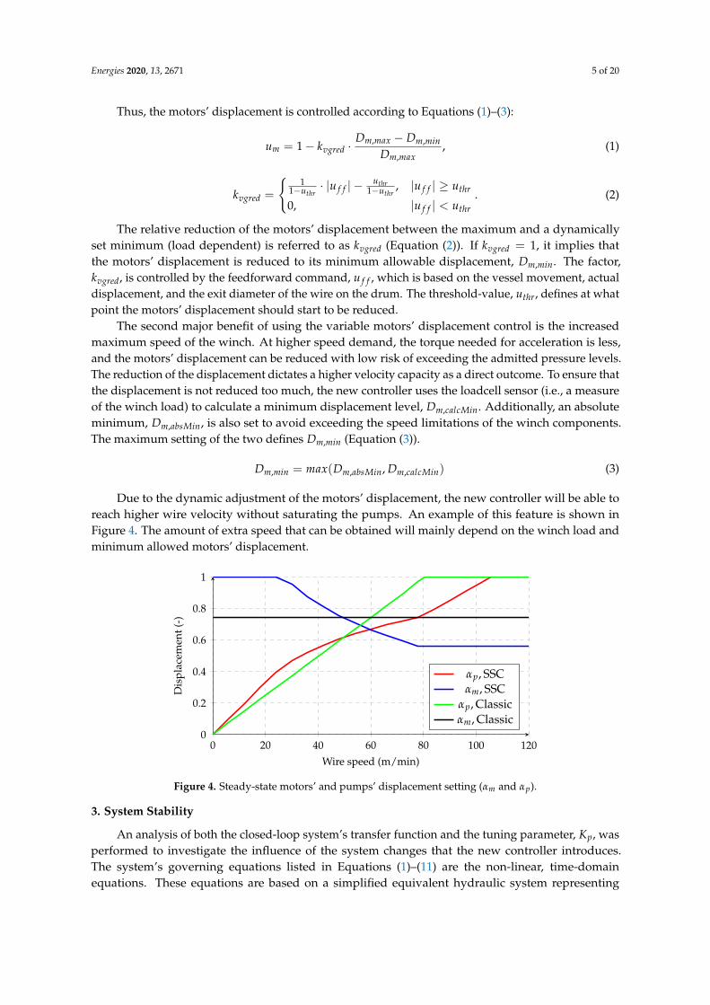
Due to the dynamic adjustment of the motors’ displacement, the new controller will be able toreach higher wire velocity without saturating the pumps. An example of this feature is shown inFigure 4. The amount of extra speed that can be obtained will mainly depend on the winch load andminimum allowed motors’ displacement.

0 20 40 60 80 100 1200

0.2

0.4

0.6

0.8

1

Wire speed (m/min)

Dis

plac

emen

t(-)

αp, SSCαm, SSC

αp, Classicαm, Classic

Figure 4. Steady-state motors’ and pumps’ displacement setting (αm and αp).

3. System Stability

An analysis of both the closed-loop system’s transfer function and the tuning parameter, Kp, wasperformed to investigate the influence of the system changes that the new controller introduces.The system’s governing equations listed in Equations (1)–(11) are the non-linear, time-domainequations. These equations are based on a simplified equivalent hydraulic system representing

Energies 2020, 13, 2671 6 of 20

the active part in the active/passive hydraulic system seen in Figure 1. The controller algorithmdescribed in Equations (1) and (2), where Equation (1) defines the motors’ control signal, um.

u f f = (k1 · vtip + k2 · atip) · Kwire · αm (4)

e =∫(vtip −

ωm · dD,max

ihD · 2 · Kwire) · dt (5)

up = u f f + Kp · e (6)

αm = w2nm · (um − αm)− 2 · ζm · wnm · αm (7)

αp = w2np · (up − αp)− 2 · ζp · wnp · αp (8)

vw =ωm · dD,max

ihD · 2 · Kwire(9)

Jme f f · ωm = Dm,max · (pA − pB) · αm − Bv ·ωm (10)VAβ· ( pA − pB) = Dp,max ·ωp · αp − αm · Dm,max ·ωm − Kleak · (pA − pB) (11)

The motors’ control signal depends on the feedforward control signal, u f f , from the crane’s tip motionand winch geometry shown in Equation (4). The position control error, calculated in Equation (5),is used with a proportional controller and a feedforward command to control the pumps (Equation (6)).The second-order equations in Equations (7) and (8), describe the response of the pumps’ and motor’sdisplacement. Equations (9)–(11) represent the dynamics of the hydromechanical system.

When linearizing the above-mentioned set of equations, it is assumed that uthr < u f f < 1, andthe low-pressure side, pB, is kept constant. Since a linearization is performed around a steady-statevelocity, the atip will naturally disappear.

Um = − 11−Uthr

· |U f f | ·Dm,max − Dm,min

Dm,max(12)

U f f = k1 · v(ss)tip · Kwire · Am + k1 ·Vtip · Kwire · α

(ss)m (13)

s · E = Vtip −Wm · dD,max

ihD · 2 · Kwire(14)

Up = U f f + Kp · E (15)

s2 · Am = w2nm · (Um − Am)− 2 · ζm · wnm · s · Am (16)

s2 · Ap = w2np · (Up − Ap)− 2 · ζp · wnp · s · Ap (17)

Vw =Wm · dD,max

ihD · 2 · Kwire(18)

Jme f f · s ·Wm = Dm,max · (p(ss)A − pB) · Am + Dm,max · α(ss)

m · PA − Bv ·Wm (19)VAβ· PA · s = Dp,max · wp · Ap − α

(ss)m · Dm,max ·Wm − w(ss)

m · Dm,max · Am − Kleak · PA (20)

Gv(s) =Vw

Vtip(21)

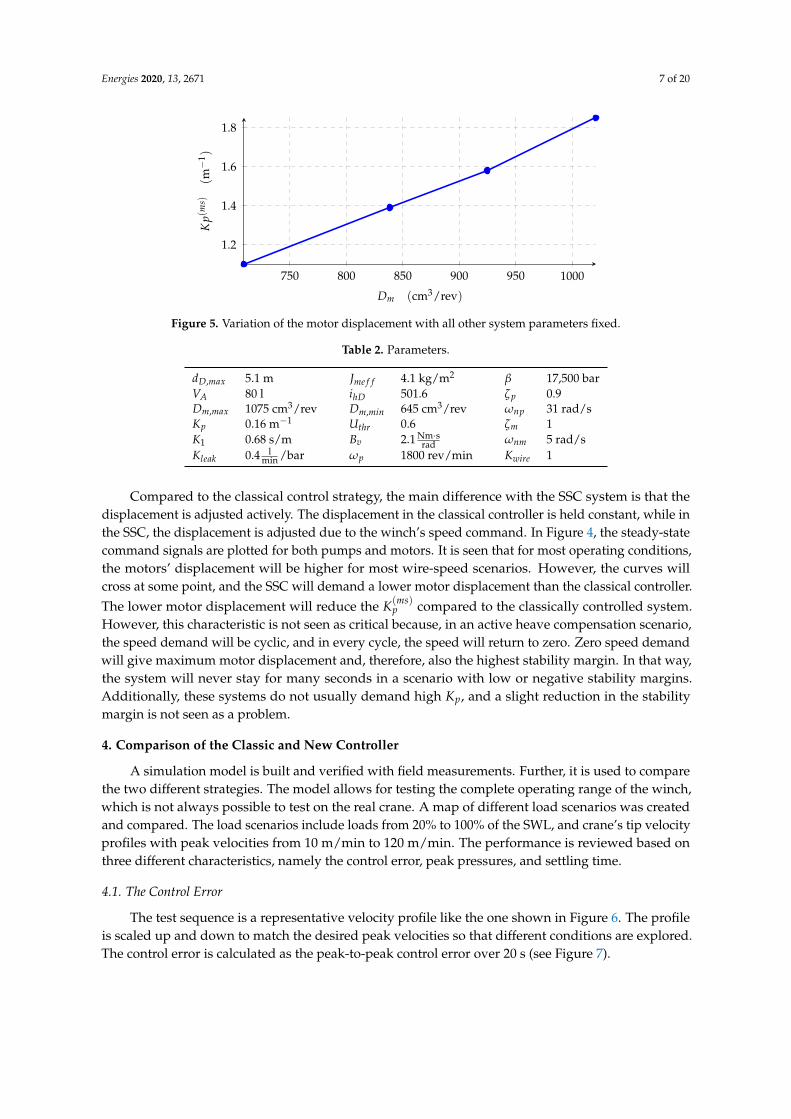
By the parameter-variation and use of the Routh-Hurwitz criterion on the transfer function Gv(s),the Kp for a marginally stable system was found, K(ms)

p . The added motor control is implementedas a pure feedforward, hence stability is not affected as long as the internal displacement controllerof the motors are stable (which is assumed in this case). Therefore, the motors’ natural frequencyand damping ratio, ωnm and ζm, have no effect on the system stability. As seen in Figure 4, the newcontroller could lead to situations with lower displacement settings than the classic controller. Basedon parameters from Table 2, Figure 5 shows the relationship between K(ms)

p and motor displacement.

Energies 2020, 13, 2671 7 of 20

750 800 850 900 950 1000

1.2

1.4

1.6

1.8

Dm (cm3/rev)

Kp(

ms)

(m−

1 )

Figure 5. Variation of the motor displacement with all other system parameters fixed.

Table 2. Parameters.

dD,max 5.1 m Jme f f 4.1 kg/m2 β 17,500 barVA 80 l ihD 501.6 ζp 0.9Dm,max 1075 cm3/rev Dm,min 645 cm3/rev ωnp 31 rad/sKp 0.16 m−1 Uthr 0.6 ζm 1K1 0.68 s/m Bv 2.1 Nm·s

rad ωnm 5 rad/sKleak 0.4 l

min /bar ωp 1800 rev/min Kwire 1

Compared to the classical control strategy, the main difference with the SSC system is that thedisplacement is adjusted actively. The displacement in the classical controller is held constant, while inthe SSC, the displacement is adjusted due to the winch’s speed command. In Figure 4, the steady-statecommand signals are plotted for both pumps and motors. It is seen that for most operating conditions,the motors’ displacement will be higher for most wire-speed scenarios. However, the curves willcross at some point, and the SSC will demand a lower motor displacement than the classical controller.The lower motor displacement will reduce the K(ms)

p compared to the classically controlled system.However, this characteristic is not seen as critical because, in an active heave compensation scenario,the speed demand will be cyclic, and in every cycle, the speed will return to zero. Zero speed demandwill give maximum motor displacement and, therefore, also the highest stability margin. In that way,the system will never stay for many seconds in a scenario with low or negative stability margins.Additionally, these systems do not usually demand high Kp, and a slight reduction in the stabilitymargin is not seen as a problem.

4. Comparison of the Classic and New Controller

A simulation model is built and verified with field measurements. Further, it is used to comparethe two different strategies. The model allows for testing the complete operating range of the winch,which is not always possible to test on the real crane. A map of different load scenarios was createdand compared. The load scenarios include loads from 20% to 100% of the SWL, and crane’s tip velocityprofiles with peak velocities from 10 m/min to 120 m/min. The performance is reviewed based onthree different characteristics, namely the control error, peak pressures, and settling time.

4.1. The Control Error

The test sequence is a representative velocity profile like the one shown in Figure 6. The profileis scaled up and down to match the desired peak velocities so that different conditions are explored.The control error is calculated as the peak-to-peak control error over 20 s (see Figure 7).

Energies 2020, 13, 2671 8 of 20

Figure 6. Velocity reference (the first 10 s are neglected due to the model initialization).

0.5 10

50

100

SWL

Velo

city

(m/m

in)

(a)

0.5 10

50

100

SWL

Velo

city

(m/m

in)

10

20

30

PPC

E(c

m)

(b)Figure 7. Maximum peak-to-peak control error (PPCE) during the test sequence: (a) Classic; (b) SSC.

The results in Figure 7, show that the classic controller has significantly reduced performancein the high-speed scenarios, and the dark-red areas displays areas where the classic controller isnot applicable. In contrast, the SSC strategy show a stable and consistent performance in the wholerange.

4.2. The Peak Pressures

The peak pressures taking place in the hydraulic system were monitored during the same cycleused for investigating the control error (see Figures 6 and 7). The maximum peak pressure depicted inFigure 8 show that for most cases the differences are small, but in favor of the SCC. The most significantpeak pressure reductions are found at velocities above 80 m/min.

0.5 10

50

100

SWL

Velo

city

(m/m

in)

(a)

0.5 10

50

100

SWL

Velo

city

(m/m

in)

100

200

300

Peak

pres

sure

(b)Figure 8. Maximum peak pressure during test sequence: (a) Classic; (b) SSC.

4.3. The Settling Time

Due to the increased motor’s displacement at low speed, the winch is expected to run smootherand give lower settling times. The settling time is tested by setting a fixed wire velocity reference andthen step up the reference velocity by 5 m/min. The settling time is defined as the amount of time

Energies 2020, 13, 2671 9 of 20

between the step command and the instant where the velocity is settled close to the target value withina certain tolerance. In this case, this tolerance is 2% of the step size (i.e., 0.1 m/min) as reported inFigure 9.

𝑇𝑖𝑚𝑒

𝑉𝑒𝑙𝑜𝑐𝑖𝑡𝑦

𝐼𝑛𝑖𝑡𝑖𝑎𝑙

𝐼𝑛𝑖𝑡𝑖𝑎𝑙+5m/min

±2% (0.1 𝑚/min)

𝑆𝑒𝑡𝑡𝑙𝑖𝑛𝑔 𝑡𝑖𝑚𝑒

Time

Velocity

Initial

Initial +5m/min

±2% (0.1 m/min)

Settling time

fig_StepSettlingTime.pdf

Figure 9. Description of the test for the settling time.

The results in Figure 10 show a significant improvement when the SSC is applied.The corresponding motors’ displacement, in Figure 11, substantiate the assumptions that improvedperformance at low speed is highly affected by the motors’ displacement. Additionally, the largedisplacement variations when using SSC is illustrated compared to the classic controller with only twofixed displacement settings.

0.5 10

50

100

SWL

Init

ialv

eloc

ity

(m/m

in)

(a)

0.5 10

50

100

SWL

Init

ialv

eloc

ity

(m/m

in)

5

Sett

ling

tim

e(s

)

(b)Figure 10. Settling time within 2% after a 5 m/min step increase of the reference velocity: (a) Classic;(b) SSC.

0.5 10

50

100

SWL

Init

ialv

eloc

ity

(m/m

in)

(a)

0.5 10

50

100

SWL

Init

ialv

eloc

ity

(m/m

in)

600

800

1000

Dis

plac

emen

t(cm

3 /re

v)

(b)Figure 11. Motors’ displacement for the results shown in Figure 10: (a) Classic; (b) SSC.

As expected, low-speed settling time characterizes the new controller. It is also seen that the newcontroller performs better at higher speeds and covers part of the map that the classical controller didnot. Additionally, it is seen that in the area where the classical controller is close to the speed limitationof the normal-speed mode, around 80 m/min, the SSC performs better.

Energies 2020, 13, 2671 10 of 20

5. Experimental Results

The full-scale tests performed on a real crane were divided into two main parts. First, the systemwas tested along a quayside with an empty hook to ensure that the overall functionality and safetycould be approved. This step included checking the motors’ displacement response and running thewinch in AHC with the simulated crane’s tip motions. Next, a second experiment was conductedoffshore with loads up to 200 tons.

5.1. The Quayside Test

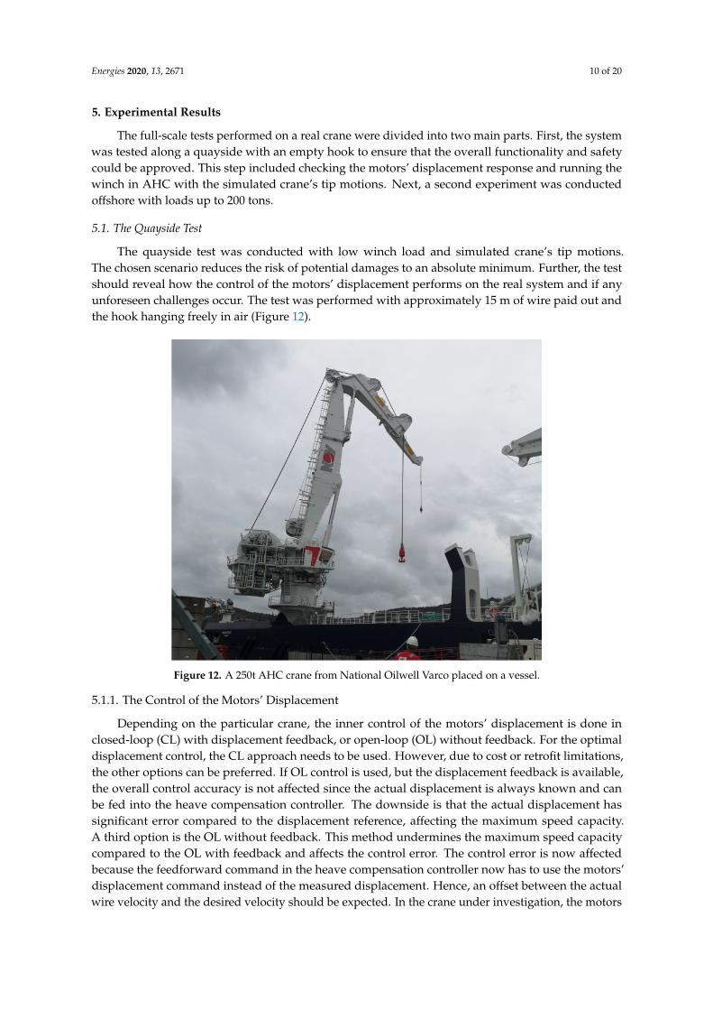
The quayside test was conducted with low winch load and simulated crane’s tip motions.The chosen scenario reduces the risk of potential damages to an absolute minimum. Further, the testshould reveal how the control of the motors’ displacement performs on the real system and if anyunforeseen challenges occur. The test was performed with approximately 15 m of wire paid out andthe hook hanging freely in air (Figure 12).

Figure 12. A 250t AHC crane from National Oilwell Varco placed on a vessel.

5.1.1. The Control of the Motors’ Displacement

Depending on the particular crane, the inner control of the motors’ displacement is done inclosed-loop (CL) with displacement feedback, or open-loop (OL) without feedback. For the optimaldisplacement control, the CL approach needs to be used. However, due to cost or retrofit limitations,the other options can be preferred. If OL control is used, but the displacement feedback is available,the overall control accuracy is not affected since the actual displacement is always known and canbe fed into the heave compensation controller. The downside is that the actual displacement hassignificant error compared to the displacement reference, affecting the maximum speed capacity.A third option is the OL without feedback. This method undermines the maximum speed capacitycompared to the OL with feedback and affects the control error. The control error is now affectedbecause the feedforward command in the heave compensation controller now has to use the motors’displacement command instead of the measured displacement. Hence, an offset between the actualwire velocity and the desired velocity should be expected. In the crane under investigation, the motors

Energies 2020, 13, 2671 11 of 20

were controlled in OL with feedback, i.e., there is always a certain discrepancy between the commandedand measured displacement, even at steady-state (Figure 13a).

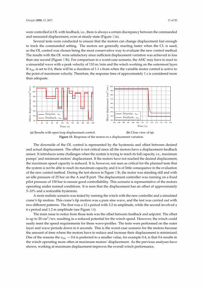
Several tests were conducted to ensure that the motors can change displacement fast enoughto track the commanded setting. The motors are generally reacting faster when the CL is used,so the OL control was chosen being the most conservative way to evaluate the new control method.The results with the OL were satisfactory since sufficient displacement variation was achieved in lessthan one second (Figure 13b). For comparison in a worst-case scenario, the AHC may have to react toa sinusoidal wave with a peak velocity of 110 m/min and the winch working on the outermost layer.If uthr is set to 0.6, there will be a duration of 1.1 s from when the variable motor control is active tothe point of maximum velocity. Therefore, the response time of approximately 1 s is considered morethan adequate.

(a) Results with open loop displacement control. (b) Close view of (a).Figure 13. Response of the motors to a displacement variation.

The downside of the OL control is represented by the hysteresis and offset between desiredand actual displacement. The offset is not critical since all the motors have a displacement feedbacksensor. It introduces some challenges when the system is trying to reach its full capacity, i.e., maximumpumps’ and minimum motors’ displacement. If the motors have not reached the desired displacement,the maximum speed capacity is reduced. It is, however, not seen as critical for the planned tests thatthe system is not be able to reach its maximum capacity, and it is of little consequence in the evaluationof the new control method. During the test shown in Figure 13b, the motor was standing still and withan idle pressure of 25 bar on the A and B port. The displacement controller was running on a fixedpilot pressure of 150 bar to ensure good controllability. This scenario is representative of the motorsoperating under normal conditions. It is seen that the displacement has an offset of approximately5–10% and a noticeable hysteresis.

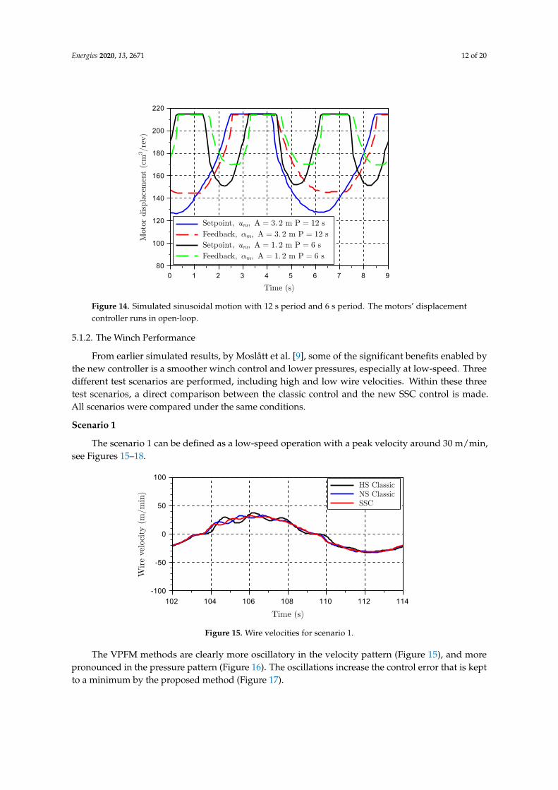
A more realistic scenario was tested by running the winch with the new controller and a simulatedcrane’s tip motion. This crane’s tip motion was a pure sine wave, and the test was carried out withtwo different patterns. The first was a 12 s period with 3.2 m amplitude, while the second involved a6 s period and 1.2 m amplitude (see Figure 14).

The main issue to notice from those tests was the offset between feedback and setpoint. The offsetis up to 20 cm3/rev, resulting in a reduced potential for the winch speed. However, the winch couldeasily meet the speed requirements for these wave-profiles. The tests were performed on the outerlayer and wave periods down to 6 seconds. This is the worst-case scenario for the motors becausethe amount of time where the motors have to reduce and increase their displacement is minimized.One of the reasons the uthr = 0.6 is preferred to a smaller value, for example 0.4, is that 0.6 results inthe winch operating more often at maximum motors’ displacement. As the previous analyses haveshown, working at maximum displacement improves the overall winch performance.

Energies 2020, 13, 2671 12 of 20

Figure 14. Simulated sinusoidal motion with 12 s period and 6 s period. The motors’ displacementcontroller runs in open-loop.

5.1.2. The Winch Performance

From earlier simulated results, by Moslått et al. [9], some of the significant benefits enabled bythe new controller is a smoother winch control and lower pressures, especially at low-speed. Threedifferent test scenarios are performed, including high and low wire velocities. Within these threetest scenarios, a direct comparison between the classic control and the new SSC control is made.All scenarios were compared under the same conditions.

Scenario 1

The scenario 1 can be defined as a low-speed operation with a peak velocity around 30 m/min,see Figures 15–18.

Figure 15. Wire velocities for scenario 1.

The VPFM methods are clearly more oscillatory in the velocity pattern (Figure 15), and morepronounced in the pressure pattern (Figure 16). The oscillations increase the control error that is keptto a minimum by the proposed method (Figure 17).

Energies 2020, 13, 2671 13 of 20

Figure 16. Pressure levels on the A-side of the active system for scenario 1.

Figure 17. Control error for scenario 1.

Figure 18. Pump and motor displacement settings for scenario 1 (0% for the motor means maximumdisplacement).

Scenario 2

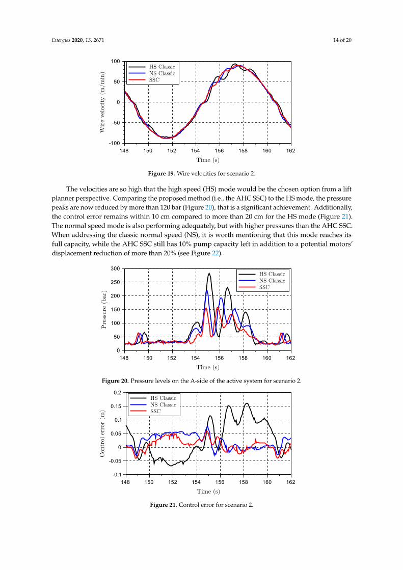
In the second scenario the peak velocity is increased to the maximum capacity for the AHCnormal speed (Figure 19).

Energies 2020, 13, 2671 14 of 20

Figure 19. Wire velocities for scenario 2.

The velocities are so high that the high speed (HS) mode would be the chosen option from a liftplanner perspective. Comparing the proposed method (i.e., the AHC SSC) to the HS mode, the pressurepeaks are now reduced by more than 120 bar (Figure 20), that is a significant achievement. Additionally,the control error remains within 10 cm compared to more than 20 cm for the HS mode (Figure 21).The normal speed mode is also performing adequately, but with higher pressures than the AHC SSC.When addressing the classic normal speed (NS), it is worth mentioning that this mode reaches itsfull capacity, while the AHC SSC still has 10% pump capacity left in addition to a potential motors’displacement reduction of more than 20% (see Figure 22).

Figure 20. Pressure levels on the A-side of the active system for scenario 2.

Figure 21. Control error for scenario 2.

Energies 2020, 13, 2671 15 of 20

Figure 22. Pump and motor displacement settings for scenario 2 (0% for the motor meansmaximum displacement).

Scenario 3

Finally, a third scenario was tested (Figures 23–26). The classic AHC HS controller is comparedagain with the AHC SSC controller.The wave pattern is made more complex with two overlyingsine waves.

Figure 23. Crane’s tip position for scenario 3.

Figure 24. Wire velocities for scenario 3.

The purpose of this modification was exploring the systems’ performance under a scenariocloser to a real-life operation. Typically, the vessel has at least two dominant frequency components.

Energies 2020, 13, 2671 16 of 20

One frequency for large swells, often related to the pitch of the vessel, and another one with a bitsmaller amplitude but higher frequency. The second frequency is, in many cases, related to the vesselroll. In this case, it was simulated as a 0.5 m amplitude with a 6 s period time on top of a 2 m amplitudewith a 13 s period time.

The results from scenario 3 are in line with the previous ones and confirm that the AHC SSC hasobvious advantages concerning controllability in the form of reduced oscillations for most conceivableworking scenarios. The pressure levels are lowered (Figure 25), and the control error (Figure 26)is minimized.

Figure 25. Pressure levels on the A-side of the active system for scenario 3.

Figure 26. Control error for scenario 3.

5.2. Discussion of the Results

The results from the field tests are shown to be very much in line with the previously simulatedresults. From the empty hook tests at the quayside, the motors’ displacement control was confirmedto behave sufficiently well due to the acceptable response time. The positive effects of keeping ahigh displacement setting at low speed were confirmed since the classic controller lead to higher andmore oscillatory pressures and winch motion, especially at low speeds shown in Figures 16 and 17.This trend was also confirmed with the mapped results from simulations in Section 4. From thedifferent maps, it is seen that the new controller expands the range of the AHC system in terms ofboth high velocity and high load scenarios. The performance has also been slightly improved, wherenormal speed mode is working close to its maximum velocity potential. Further, it is discoveredthat the peak pressures are reduced, especially for scenarios with high wire velocities. Additionally,the low-speed performance is improved (it was measured by the use of the settling time after a step

Energies 2020, 13, 2671 17 of 20

command in the velocity reference). Concerning the crane tested in field, it was not possible to gainany extra speed compared to the classic HS controller due to gearbox speed limitations. Nevertheless,the AHC SSC controller enables higher load capacity and better winch performance. For the offshoretesting, the results were similar, although it was not possible to compensate with higher velocities than40m/min due to the weather conditions (40 m/min is below 50% of the rated winch capacity). The theresults were still positive leading to reduced peak pressures and reduced oscillations. The classic HSmode was also tested offshore. The tests, not displayed in this paper, confirmed the same satisfactorybehavior that was seen during the quayside tests.

6. Conclusions

The newly developed semi secondary control (SSC) method for offshore heave compensatedwinches has been investigated and compared to the current state-of-the-art approach with a fixedsetting of the motors’ displacement. Firstly, it has been shown that the SSC leads to variations in themarginal stability because of the variations in the motor displacement, but, higher stability margins areachieved compared to the the classical control method at low speeds. Secondly, the increased windowof operations expected from the SSC has been verified by comparing the peak-to-peak position error,peak pressure, and settling time for variations in both the payload and reference motion. Finally,the improved dynamic performance has been experimentally verified by means of full scale tests on a250 ton crane.

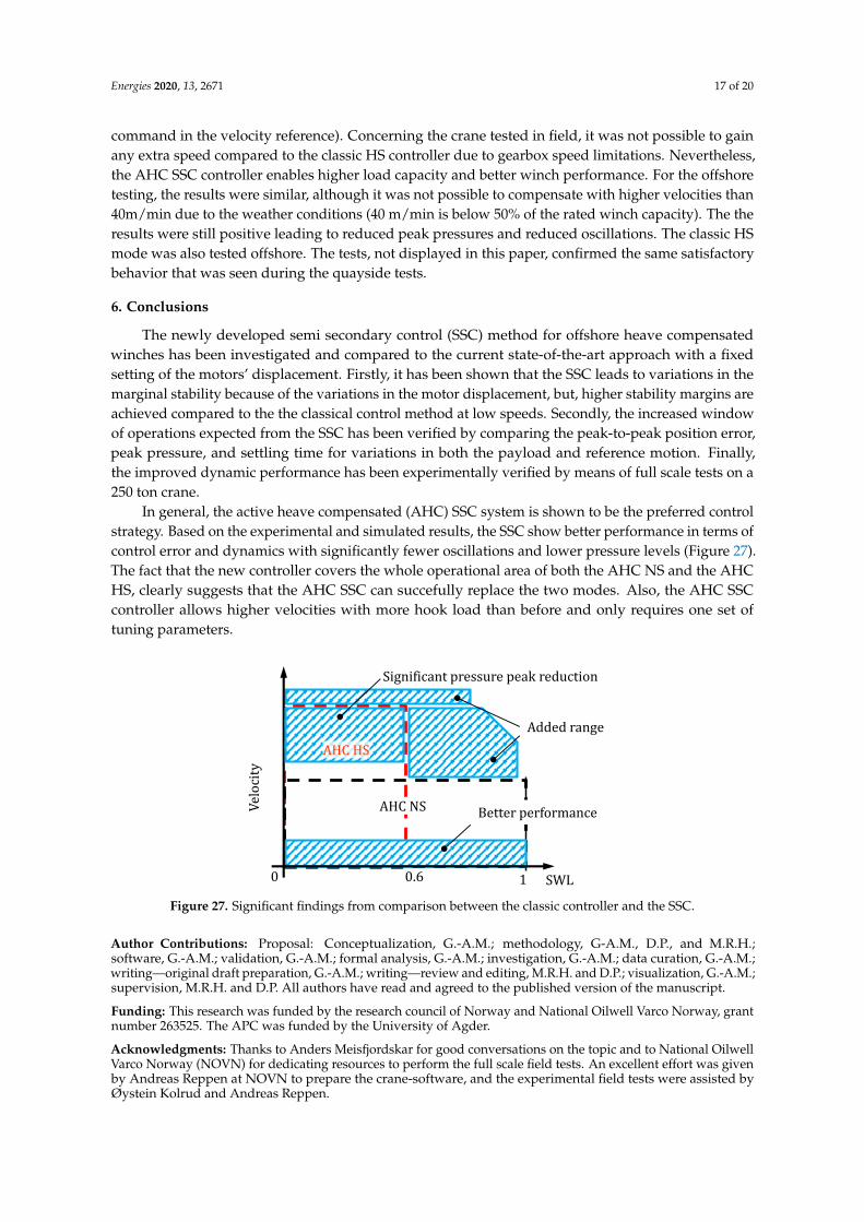
In general, the active heave compensated (AHC) SSC system is shown to be the preferred controlstrategy. Based on the experimental and simulated results, the SSC show better performance in terms ofcontrol error and dynamics with significantly fewer oscillations and lower pressure levels (Figure 27).The fact that the new controller covers the whole operational area of both the AHC NS and the AHCHS, clearly suggests that the AHC SSC can succefully replace the two modes. Also, the AHC SSCcontroller allows higher velocities with more hook load than before and only requires one set oftuning parameters.

SWL1

Added range

0 0.6

Velocity

AHC NS Better performance

Significant pressure peak reduction

fig_improvements_AHC3

AHC HS

Figure 27. Significant findings from comparison between the classic controller and the SSC.

Author Contributions: Proposal: Conceptualization, G.-A.M.; methodology, G-A.M., D.P., and M.R.H.;software, G.-A.M.; validation, G.-A.M.; formal analysis, G.-A.M.; investigation, G.-A.M.; data curation, G.-A.M.;writing—original draft preparation, G.-A.M.; writing—review and editing, M.R.H. and D.P.; visualization, G.-A.M.;supervision, M.R.H. and D.P. All authors have read and agreed to the published version of the manuscript.

Funding: This research was funded by the research council of Norway and National Oilwell Varco Norway, grantnumber 263525. The APC was funded by the University of Agder.

Acknowledgments: Thanks to Anders Meisfjordskar for good conversations on the topic and to National OilwellVarco Norway (NOVN) for dedicating resources to perform the full scale field tests. An excellent effort was givenby Andreas Reppen at NOVN to prepare the crane-software, and the experimental field tests were assisted byØystein Kolrud and Andreas Reppen.

Energies 2020, 13, 2671 18 of 20

Conflicts of Interest: The funder, National Oilwell Varco Norway, had a role in the design of the study; in thecollection, analyses, and interpretation of data; in the writing of the manuscript, and in the decision to publishthe results.

Abbreviations

αm Motor displacement feedbackαp Pump displacement feedbackωm Rotational velocity of motor shaftωnm Natural eigenfrequency of motor displacement controlωnp Natural eigenfrequency of pump displacement controlζm Damping ratio of motor displacement controlζp Damping ratio of pump displacement controlAm Laplace transform of αm

Am Laplace transformed αm

Ap Laplace transform of αp

Ap Laplace transformed αp

atip Crane tip accelerationdD,max Maximum drum diameterDm,max Maximum motor displacementDm,min Minimum allowable motor displacementE Laplace transform of ee Controller errorihD Transmission ratio between hydraulic motor shaft rotation and drumJme f f Total inertia on motor shaftk1 Proportional gain for crane tip velocity in feedforward controllerk2 Proportional gain for crane tip acceleration in feedforward controllerKleak Laminar leakage factorKp Proportional gain for feedback control errorkvgred Factor for motor displacement reductionKwire Drum diameter factorPA Laplace transform of pApA Pressure A sidepB Pressure B sideU f f Laplace transform of u f fU f f Laplace transformed u f fu f f Feedforward signalUm Laplace transform of um

Um Laplace transformed um

um Command signal for motor displacement controlUp Laplace transform of up

up Command signal for pump displacement controlUthr Laplace transform of uthruthr Threshold value for when to start reducing motor displacementVtip Laplace transform of vtipVtip Laplace transformed vtipvtip Crane tip velocityVw Laplace transform of vw

Vw Laplace transformed vw

vw Wire velocityWm Laplace transform of ωm

Energies 2020, 13, 2671 19 of 20

AHC Active heave compensationAHC HS Active heave compensation, high-speed modeAHC NS Active heave compensation, normal speed modeFTC Fault tolerant controlHST Hydrostatic transmissionMPC Model-based controlNOV National Oilwell VarcoVPFM Variable pumps and fixed motorsVPVM Variable pumps and variable motorsSSC Semi secondary controlSWL Safe working load

References

1. Woodacre, J.K.; Bauer, R.J.; Irani, R.A. A review of vertical motion heave compensation systems. Ocean Eng.2015, 104, 140–154. [CrossRef]

2. Feuser, A. Hydrostatic Drives with Control of the Secondary Unit; Mannesmann Rexroth GmbH: Lohr am Main,Germany, 1989; Volume 6.

3. Palmgren, G.; Rydberg, K.E. Secondary Controlled Systems—Energy Aspects and Control Strategies.In Proceedings of the International Conference on Fluid Power, Tampere, Finland, 24–26 March 1987.

4. Bosch Rexroth AG. Drive and Control Solutions for Marine Engineering: Reliable, Efficient, Durable; RexrothBosch B.V., Netherlands. Available online: https://dc-us.resource.bosch.com/media/us/products_13/product_groups_1/industrial_hydraulics_5/\pdfs_4/R999001175_2015-1.pdf (accessed on 24 May 2020).

5. Marien, M.; Wiig, K.E.; Ebbesen, M.K. Secondary Control of a Digital Hydraulic Motor for WinchApplications. Master’s Thesis, University of Agder, Kristiansand S, Norway, 2018.

6. Padovani, D.; Ivantysynova, M. The Concept of Secondary Controlled Hydraulic Motors Applied to thePropulsion System of a Railway Machine. In Proceedings of the 14th Scandinavian International Conferenceon Fluid Power, Tampere, Finland, 20–22 May 2015.

7. Padovani, D.; Ivantysynova, M. Simulation and Analysis of Non-Hybrid Displacement-Controlled HydraulicPropulsion Systems Suitable for Railway Applications. In Proceedings of the ASME/BATH 2015 Symposiumon Fluid Power and Motion Control, Chicago, IL, USA, 12–14 October 2015; p. 11. [CrossRef]

8. Nikolaus, H. Antriebssystem mit hydrostatischer Kraftubertragung. Patent number 27,399,684, 1977.9. Moslått, G.A.; Padovani, D.; Hansen, M.R. A Control Algorithm for Active/Passive Hydraulic Winches

Used in Active Heave Compensation. In Proceedings of the ASME/BATH 2019 Symposium on Fluid Powerand Motion Control; American Society of Mechanical Engineers: Sarasota, FL, USA, 7–9 October 2019; p. 11.[CrossRef]

10. Kaddissi, C.; Kenne, J.P.; Saad, M. Identification and Real-Time Control of an Electrohydraulic Servo System Basedon Nonlinear Backstepping. IEEE/ASME Trans. Mechatron. 2007, 12, 12–22. [CrossRef]

11. Yao, J.; Jiao, Z.; Ma, D. Extended-state-observer-based output feedback nonlinear robust control of hydraulicsystems with backstepping. IEEE Trans. Ind. Electron. 2014, 61, 6285–6293. [CrossRef]

12. Mahulkar, V.; Adams, D.E.; Derriso, M. Adaptive fault tolerant control for hydraulic actuators. In Proceedingsof the American Control Conference, American Automatic Control Council, Chicago, IL, USA, 1–3 July 2015;Volume 2015, pp. 2242–2247. [CrossRef]

13. Yao, J.; Jiao, Z.; Ma, D.; Yan, L. High-accuracy tracking control of hydraulic rotary actuators with modelinguncertainties. IEEE/ASME Trans. Mechatron. 2014, 19, 633–641. [CrossRef]

14. Yao, B.; Bu, F.; Reedy, J.; Chiu, G.T. Adaptive robust motion control of single-rod hydraulic actuators: Theoryand experiments. IEEE/ASME Trans. Mechatron. 2000, 5, 79–91. [CrossRef]

15. Yao, J.; Deng, W.; Jiao, Z. Adaptive control of hydraulic actuators with LuGre model-based frictioncompensation. IEEE Trans. Ind. Electron. 2015, 62, 6469–6477. [CrossRef]

16. Yao, J.; Jiao, Z.; Ma, D. A Practical Nonlinear Adaptive Control of Hydraulic Servomechanisms with Periodic-LikeDisturbances. IEEE/ASME Trans. Mechatron. 2015, 20, 2752–2760. [CrossRef]

17. Do, H.T.; Ahn, K.K. Velocity control of a secondary controlled closed-loop hydrostatic transmission systemusing an adaptive fuzzy sliding mode controller. J. Mech. Sci. Technol. 2013, 27, 875–884. [CrossRef]

Energies 2020, 13, 2671 20 of 20

18. Meller, M.; Kogan, B.; Bryant, M.; Garcia, E. Model-based feedforward and cascade control of hydraulicMcKibben muscles. Sens. Actuators A Phys. 2018, 275, 88–98. [CrossRef]

19. Chatzakos, P.; Papadopoulos, E. On model-based control of hydraulic actuators. Proc. RAAD 2003, 3, 7–10.20. Rezayi, S.; Arbabtafti, M. A New Model-Based Control Structure for Position Tracking in an Electro-Hydraulic

Servo System with Acceleration Constraint. J. Dyn. Syst. Meas. Control 2017, 139. [CrossRef]21. Guan, C.; Pan, S. Adaptive sliding mode control of electro-hydraulic system with nonlinear unknown

parameters. Control Eng. Pract. 2008, 16, 1275–1284. [CrossRef]22. Zheng, S.; Wang, X.; Lu, Y.; Wang, Y. The sliding mode control for speed system of the variable displacement

motor at the constant pressure network. In Proceedings of the 2013 International Conference on IntelligentControl and Information Processing, ICICIP 2013, Beijing, China, 9–11 June 2013; pp. 499–503. [CrossRef]

23. Liu, S.; Guo, Q.; Zhao, W. Research on active heave compensation for offshore crane. In Proceedings ofthe 26th Chinese Control and Decision Conference, CCDC 2014, Changsha, China, 31 May–2 June 2014;pp. 1768–1772. [CrossRef]

24. Shi, M.; Guo, S.; Jiang, L.; Huang, Z. Active-Passive Combined Control System in Crane Type for HeaveCompensation. IEEE Access 2019, 7, 159960–159970. [CrossRef]

25. Michel, A.; Kemmetmüller, W.; Kugi, A. Modeling and control of an active heave compensation system foroffshore cranes. At-Automatisierungstechnik 2012, 60, 8–15. [CrossRef]

26. Sanders, R. Modelling and Simulation of Traditional Hydraulic Heave Compensation Systems; Technical Report;University of Twente, Faculty of Engineering Technology: Enschede, The Netherlands, 2016.

27. Wu, J.; Wu, D. Integrated design of an active heave compensation crane with hydrostatic secondary control.In Proceedings of the OCEANS 2018 MTS/IEEE Charleston, OCEAN 2018, Charleston, SC, USA, 22–25October 2018; pp. 1–7. [CrossRef]

28. Donkov, V.; Andersen, T.; Ebbesen, M.K.; Linjama, M.; Paloniitty, M. Investigation of the fault toleranceof digital hydraulic cylinders. In Proceedings of the 16th Scandinavian International Conference on FluidPower, Tampere, Finland, 22–24 May 2019.

29. Dijoux, E.; Steiner, N.Y.; Benne, M.; Péra, M.C.; Pérez, B.G. A review of fault tolerant control strategiesapplied to proton exchange membrane fuel cell systems. J. Power Sources 2017, 359, 119–133. [CrossRef]

30. Küchler, S.; Mahl, T.; Neupert, J.; Schneider, K.; Sawodny, O. Active control for an offshore crane using predictionof the vessels motion. IEEE/ASME Trans. Mechatron. 2011, 16, 297–309. [CrossRef]

31. Kusters, J.G.; Cockrell, K.L.; Connell, B.S.; Rudzinsky, J.P.; Vinciullo, V.J. FutureWavesTM: A real-time Ship MotionForecasting system employing advanced wave-sensing radar. In Proceedings of the OCEANS 2016 MTS/IEEEMonterey, OCE 2016, Monterey, CA, USA, 19–23 September 2016; pp. 1–9. [CrossRef]

32. Del Re, L.; Goransson, A.; Astolfi, A. Enhancing Hydrostatic Gear Efficiency Through Nonlinear OptimalControl Strategies. J. Dyn. Syst. Meas. Control 1996, 118, 727–732. [CrossRef]

c© 2020 by the authors. Licensee MDPI, Basel, Switzerland. This article is an open accessarticle distributed under the terms and conditions of the Creative Commons Attribution(CC BY) license (http://creativecommons.org/licenses/by/4.0/).