Under review with Int. J. Non-linear Mechanics

Performance improvement through passive mechanics in

jellyfish-like swimming

Megan M. Wilson1 and Jeff D. Eldredge2

Mechanical & Aerospace Engineering Department

University of California, Los AngelesLos Angeles, CA 90095, USA

24 March 2010

Abstract

This computational investigation explores the effect that passively responsive com-

ponents of a body can have on swimming performance. The swimmer is an articulated

two-dimensional system of linked rigid bodies that is prescribed with a reciprocating

shape change inspired by jellyfish mechanics. The six constituent hinges can be ei-

ther actively controlled by fully prescribing the kinematics, or passively responsive by

substituting a torsion spring in place of an actuator. The computational solver is a

high-fidelity viscous vortex particle method with coupled fluid-body interactions. The

prescribed kinematic Reynolds numbers involved in this investigation fall within the

range 70 to 700. Several configurations are explored, including cases with passively

responsive hinges and cases in which pairs of the hinges were held in a rigid locked

position. Certain choices of passive structure lead to optimal swimming speed and effi-

ciency. This is elucidated by a simple model, which shows that optimal performance is

obtained through a balance of maximized deflection of peripheral bodies and phasing

that draws benefits from both reactive and resistive force mechanisms. A study is also

made of an inviscid swimmer but, due to the reciprocating kinematics of the system,

the swimmer is unable to achieve meaningful locomotion, showing that vortex shedding

is essential to break the symmetry of the kinematics.

1 Introduction

Creatures immersed in fluids often make use of flexibility to aid in locomotion. For example,in insect flight, wing pitch reversal at the end of a stroke is aided by passive mechanismsincluding aerodynamic torque and the inertia of the wing itself rather than being fullyactively controlled by muscles [1, 2], and in some optimized instances the wing pitch reversalwas found to be entirely passive. Eldredge and Toomey demonstrated that a wing withchordwise flexibility is less sensitive to the phase between pitching and heaving compared

1meganwils@ucla.edu2eldredge@seas.ucla.edu

1

to a rigid counterpart, but that performance of the flexible wing can be adversely affectedby premature shedding of the leading-edge vortex [3, 4]. Using a similar system, Vanellaet al. showed that aerodynamic performance is enhanced as the linear flapping frequencyapproaches one of the non-linear frequencies of the flexible system [5].

For swimmers, the effects of passive flow control have been investigated in relation to themorphology of the body itself [6, 7]. There have also been studies looking into the activedeformation of an elastic fin under external loading by the surrounding fluid [8]. However,few have attempted to determine the energy savings that can be obtained through elasticstrain energy stored in the system. Biological swimmers are known to take advantage ofenergy savings obtained through the elastic response of tendons and muscular tissues [9].The flexible flukes of dolphins and whales are known to increase swimming performance[10, 11].

Oblate medusan swimmers have been the target of many recent investigations, bothexperimental [12, 13, 14, 15, 16, 17, 18] and computational [19, 20, 21, 22]. Such swimmersare composed of muscular filaments that circumscribe the body [23, 24]. Power is deliveredfrom the muscles during contraction, during which elastic strain energy is stored and isreleased during the refilling portion of the cycle [25]. It has been shown that jet-poweredinvertebrates use elastic springs in parallel with muscular tissues to power half of theirlocomotor cycle [26, 27].

It is of interest to distill these biological problems into simplified mechanical problemsthat can more easily be studied. The passive flapping of a flag has been the subject ofseveral recent investigations [28, 29], and serves as a useful model with which to understandenergy extraction from a uniform free stream. The drag reduction achievable from an elasticstructure has been studied by examining the bending of a flexible filament normal to auniform flow [30, 31].

In this work, we distill the structure of an oblate medusan swimmer into a simple modelwith which we can explore passive swimming mechanics. We forego any attempt to modelthe structure of the creature precisely. Rather, we focus on a two-dimensional system oflinked rigid bodies. The objective is not to understand the biological problem per se, butto explore the effect of bio-inspired passive mechanics generically. In contrast to the parallelarrangement of muscular tissues in medusan organisms, this study investigates the effect ofpassively responsive components arranged in series with active mechanisms.

For a system of linked rigid bodies, passively responsive hinges modeled as torsion springscapture and store elastic strain energy as they are deflected and release energy as theyrecoil. The present investigation focuses on the performance benefits obtained from theseenergy savings. Oblate medusa-like swimmers, in general, are not effective swimmers andare able to propel themselves only because of vorticity produced at the rim of the bell[13, 32]. We approach this investigation using a high-fidelity viscous solver [33], which isthen complemented with an inviscid solution in which vorticity is not produced.

The section describing the target problem includes the geometric parameters, kinematics,and the control scheme of the model. This is followed by a summary of the numericalmethod, as well as the metrics used to determine the power requirements and the efficiencyof the swimmer. The results section includes a discussion of the effect of the kinematicReynolds number on locomotion with fully prescribed kinematics, the effects of allowinghinges to passively respond as well as remain in a locked position, and finally, the behavior

2

Y/

L

X/ L

0.2

-0.8

-0.6

-0.4

-0.2

0.0

0.5 1.0-0.5-1.0 0.0

Y/

L

X/ L

0.2

-0.8

-0.6

-0.4

-0.2

0.0

0.5 1.0-0.5-1.0 0.0

1

2

3 4

5

6

−θ1

H

D

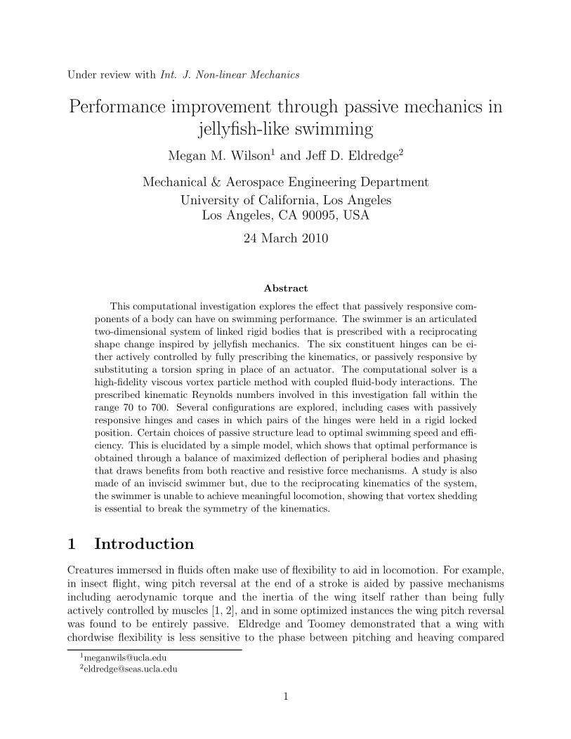
Figure 1: Simplified jellyfish kinematic model: (Left) projected outline and centerline of thejellyfish from experimental data [13], with marker points (•) used for generating articulatedmodel; (Right) articulated system of linked rigid bodies and numbering system used forhinges. H and D denote the height and diameter of the model, respectively [19].

of a passively responsive inviscid swimmer. The study is completed with an analysis andprediction of the optimal swimming performance with a simple linear model for the peripheralconstituent bodies.

2 Materials and methods

2.1 Target problem

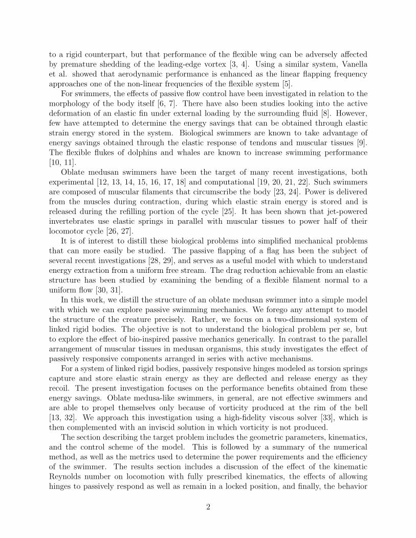
The target of this study, which was also previously studied by Wilson et al [19], is a two-dimensional articulated system that is representative of oblate hydromedusae, shown inFigure 1. The rigid body system consists of seven constituent bodies and approximates thecenterline of the silhouette of the jellyfish [34, 13]. Five marker points were tracked overtwo contraction cycles and the secants joining these points were used to divide the centerlineinto discrete links modeled as neutrally buoyant rigid elliptical bodies. The lengths of theseconstituent bodies were equivalent to the mean lengths of the corresponding secant, howeverthis simplified representative model did not account for the thickness of the actual organism.The prescribed hinge kinematics were obtained by plotting the angles between these secantsfrom a sequence of snapshots of the outline of this jellyfish body over these two contractioncycles, shown in Figure 2, and each was fitted with a sinusoidal curve. Left-right symmetrywas enforced for both the system structure and the prescribed kinematics, but was notenforced during the simulation.

The first relevant length scale inherent to this problem is the effective swimming arm L,which is used to scale the coordinates. The swimming arm is defined as the arc length fromthe orifice lip to the innermost hinge (hinge 3). Two additional length scales become apparentonce the kinematics are applied: the mean ‘height’ of the bell H , where H/L ≈ 0.67, andthe maximum diameter of the bell Dmax, where Dmax/L ≈ 2.1. The undulation period, T ,is comprised of both the contraction phase and the relaxation phase, which forms a naturaltime scale for the problem. Resulting from the prescribed hinge actuation, the largest speedin the problem occurs at the orifice lip, where |Ulip|max ≈ 1.5L/T relative to the center

3

0 0.2 0.4 0.6 0.8 1.0 1.2 1.4 1.6 1.8 2.0

0

0.5

1.0

θ1 (

rad

)

t/T

0

0.5

1.0

0

0.5

1.0

θ2 (

rad

)θ

3 (

rad

)

Figure 2: Measured angles (•) and sinusoidal hinge correlations for hinges 1 through 3 [19].

constitutive body.There are two relevant Reynolds numbers: one based on the prescribed hinge kinematics

and the other based on the resulting self-propulsion. The kinematic Reynolds number ReK

is based on the maximum bell diameter and the undulation period and is defined as ReK =D2

max/Tν, where ν is the kinematic viscosity. The kinematic Reynolds numbers used inthis investigation are 70 ≤ ReK ≤ 700. Noting a slightly different definition based on themaximum speed at the orifice lip and the mean ‘height’ of the bell, ReK2 = |Ulip|maxH/ν,the relevant kinematic Reynolds numbers are 16 ≤ ReK2 ≤ 160. The propulsion Reynoldsnumber, ReP = VcH/ν, is determined during the course of the simulation and is based onthe mean longitudinal speed of the centroid of the jellyfish Vc and the mean height of thebell.

Pairs of hinges were designated to be passively responsive by modeling the hinges astorsion springs with no active input. The equilibrium angle of the spring, θe, was set to themean angle, θ, of the corresponding active control kinematics for that specific hinge. Allelastic hinges have the same initial hinge angle as the fully prescribed case, θo; thus, everycase begins with exactly the same body shape at time t = 0. A range of stiffness coefficientswas tested, all with zero damping.

In some cases, the innermost hinges (hinges 3 and 4) were fixed in a locked position atangle θe. Unlike the passively responsive cases, these locked hinges do not begin at the sameinitial angle as the fully actuated case, θo, but rather at θe. The effect of this differencein the initial body shape is negligible. These cases were explored in recognition of the lowamplitude of these hinges in the actively prescribed kinematics, as evident in Figure 2.

It has been shown that articulated systems of linked rigid bodies can propel themselvesby altering their shape, even in a perfect fluid [35, 36], demonstrating that some forms oflocomotion can be achieved by a biologically inspired swimmer in the absence of vortexshedding. In such cases, the inviscid swimmer is found to propel itself more rapidly than itsviscous counterpart [37], but the behavior of the swimmers is qualitatively similar. For sucha swimmer to be effective in an inviscid setting, the kinematics must be non-reciprocating,i.e. the body shape change must be distinct when performed in reverse [38]. Here, the

4

kinematics of the medusan swimmer are nearly reciprocating. Its performance in an inviscidfluid is therefore expected to be poor.

2.2 Numerical methodology

The numerical simulations were carried out with a viscous vortex particle method, withstrong coupling to the body dynamics. Compared to a grid-based method, implementinga particle method is advantageous because it is able to adapt to the constantly changingbody configuration naturally and only requires particles to be tracked in regions in whichthe vorticity is non-zero, thus reducing the computational domain. For more details on thishigh-fidelity method, the reader is referred to previous work [33, 39].

2.3 Power and efficiency considerations

The components of power associated with an articulated system of n linked rigid bodiescan be calculated directly from the simulation results. Given the fluid forces, F fi

, and fluidmoment, Mfi

, on the individual bodies (where i = 1, . . . , n), the power resulting from thework done by the fluid on the system of bodies, Wf , can be found using

Wf =n

∑

i=1

(Ffi· xi + Mfi

αi) (1)

where xi is the rate of change of the body centroid and αi is the angular velocity of body i.There are n−1 hinges in the system, and the rate of change of energy stored and released

as they are deflected, Es, is

Es =n−1∑

i=1

ki(θi − θei)θi (2)

where ki is the stiffness of hinge i.The rate of change of kinetic energy of the system of bodies is

Eb =n

∑

i=1

(Ai(xi · xi) + Jiαiαi) (3)

where Ai is the area and Ji is the polar moment of inertia of body i.Thus, the total power required to activate the hinges, Wh, is given by

Wh = Es + Eb − Wf . (4)

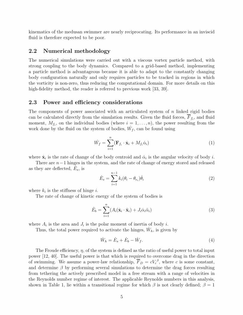
The Froude efficiency, η, of the system is defined as the ratio of useful power to total inputpower [12, 40]. The useful power is that which is required to overcome drag in the directionof swimming. We assume a power-law relationship, F D = cVc

β , where c is some constant,and determine β by performing several simulations to determine the drag forces resultingfrom tethering the actively prescribed model in a free stream with a range of velocities inthe Reynolds number regime of interest. The applicable Reynolds numbers in this analysis,shown in Table 1, lie within a transitional regime for which β is not clearly defined; β = 1

5

10−3 10−2 10−110−3

10−2

10−1

Vc

Fd

Figure 3: Power law analysis to determine constant β using a linear fit to data ().

for very low Reynolds numbers and β = 2 for high Reynolds numbers. As Figure 3 shows,it was found that β ≈ 1 for this analysis, or in other words, F D ∼ Vc. Thus, the efficiencyis given by

η =cVc

2

W h

. (5)

This is, in turn, is normalized by the efficiency of the active swimmer, to determine an‘effectiveness’

η

ηactive=

cVc2/Wh

(cVc2/Wh)active

=Vc

2/Wh

(Vc2/Wh)active

. (6)

3 Results

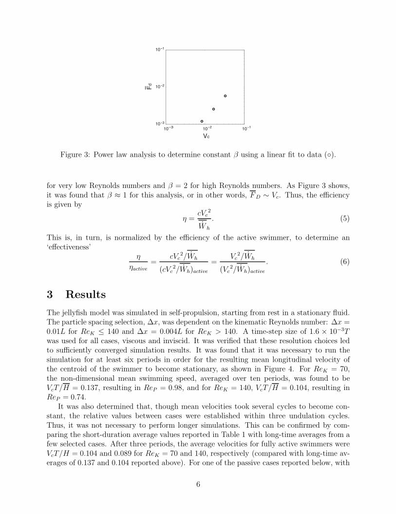
The jellyfish model was simulated in self-propulsion, starting from rest in a stationary fluid.The particle spacing selection, ∆x, was dependent on the kinematic Reynolds number: ∆x =0.01L for ReK ≤ 140 and ∆x = 0.004L for ReK > 140. A time-step size of 1.6 × 10−3Twas used for all cases, viscous and inviscid. It was verified that these resolution choices ledto sufficiently converged simulation results. It was found that it was necessary to run thesimulation for at least six periods in order for the resulting mean longitudinal velocity ofthe centroid of the swimmer to become stationary, as shown in Figure 4. For ReK = 70,the non-dimensional mean swimming speed, averaged over ten periods, was found to beVcT/H = 0.137, resulting in ReP = 0.98, and for ReK = 140, VcT/H = 0.104, resulting inReP = 0.74.

It was also determined that, though mean velocities took several cycles to become con-stant, the relative values between cases were established within three undulation cycles.Thus, it was not necessary to perform longer simulations. This can be confirmed by com-paring the short-duration average values reported in Table 1 with long-time averages from afew selected cases. After three periods, the average velocities for fully active swimmers wereVcT/H = 0.104 and 0.089 for ReK = 70 and 140, respectively (compared with long-time av-erages of 0.137 and 0.104 reported above). For one of the passive cases reported below, with

6

0-0.2

0

0.2

0.4

2 4 6 8 10 12

t/T

Vc T

/ H

Figure 4: Longitudinal centroid velocity profile of viscous self propelling swimmers with fullyprescribed kinematics for ReK = 70 (—) and ReK = 140 (– –).

ReK = 70 and a spring of stiffness k = 0.005 in the first and sixth hinge, the three-periodaverage is Vc = 0.122 and the long-time average is 0.150. Thus, although the mean speed ofthe swimmers has not reached steady state, the relative mean velocities between the casesremain approximately constant. This observation allowed the simulations to be run overa shorter time interval, 3T , and by normalizing the results, it was possible to predict thecomparative behavior of the systems under various imposed conditions.

3.1 Fully prescribed kinematics

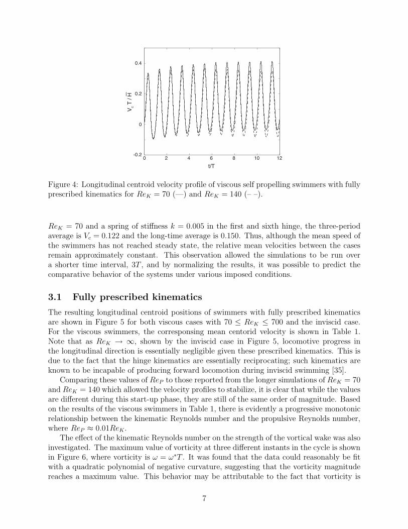
The resulting longitudinal centroid positions of swimmers with fully prescribed kinematicsare shown in Figure 5 for both viscous cases with 70 ≤ ReK ≤ 700 and the inviscid case.For the viscous swimmers, the corresponsing mean centorid velocity is shown in Table 1.Note that as ReK → ∞, shown by the inviscid case in Figure 5, locomotive progress inthe longitudinal direction is essentially negligible given these prescribed kinematics. This isdue to the fact that the hinge kinematics are essentially reciprocating; such kinematics areknown to be incapable of producing forward locomotion during inviscid swimming [35].

Comparing these values of ReP to those reported from the longer simulations of ReK = 70and ReK = 140 which allowed the velocity profiles to stabilize, it is clear that while the valuesare different during this start-up phase, they are still of the same order of magnitude. Basedon the results of the viscous swimmers in Table 1, there is evidently a progressive monotonicrelationship between the kinematic Reynolds number and the propulsive Reynolds number,where ReP ≈ 0.01ReK .

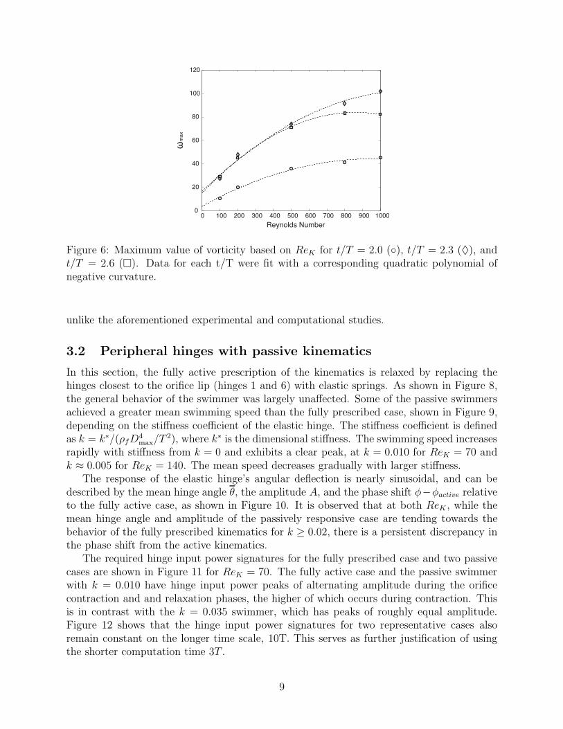
The effect of the kinematic Reynolds number on the strength of the vortical wake was alsoinvestigated. The maximum value of vorticity at three different instants in the cycle is shownin Figure 6, where vorticity is ω = ω∗T . It was found that the data could reasonably be fitwith a quadratic polynomial of negative curvature, suggesting that the vorticity magnitudereaches a maximum value. This behavior may be attributable to the fact that vorticity is

7

0 0.5 1.0 1.5 2.0 2.5 3.0−0.25

−0.20

−0.15

−0.10

−0.05

0.00

0.05

0.10

0.15

0.20

t/T

Yc / H

Figure 5: Longitudinal centroid position of self propelling swimmers with fully prescribedkinematics for: ReK = 70 (—), ReK = 140 (– –), ReK = 350 (– · –), ReK = 560 (· · ·),ReK = 700 (– ·· –), and the inviscid case (- - · - -).

ReK VcT/H ReP

70 0.104 0.74140 0.089 1.27350 0.119 4.24560 0.110 6.27700 0.107 7.62

Table 1: Non-dimensional velocity, VcT/H, and propulsive Reynolds number, ReP , for fullyactive viscous swimmers over three periods of undulation, at various kinematic Reynoldsnumbers.

generated by relative motion between the orifice lip and surrounding fluid, and this relativemotion may actually decrease with increasing ReK as the reciprocating kinematics becomemore important.

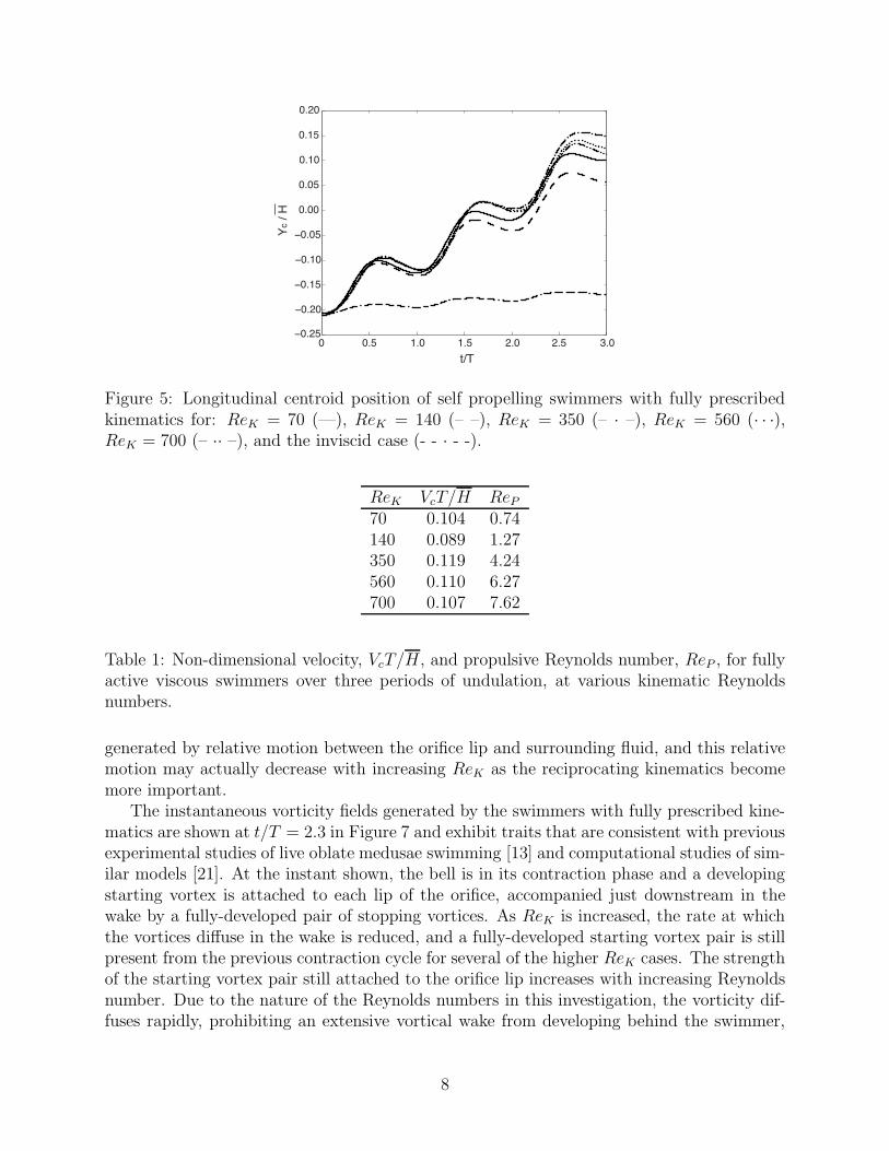
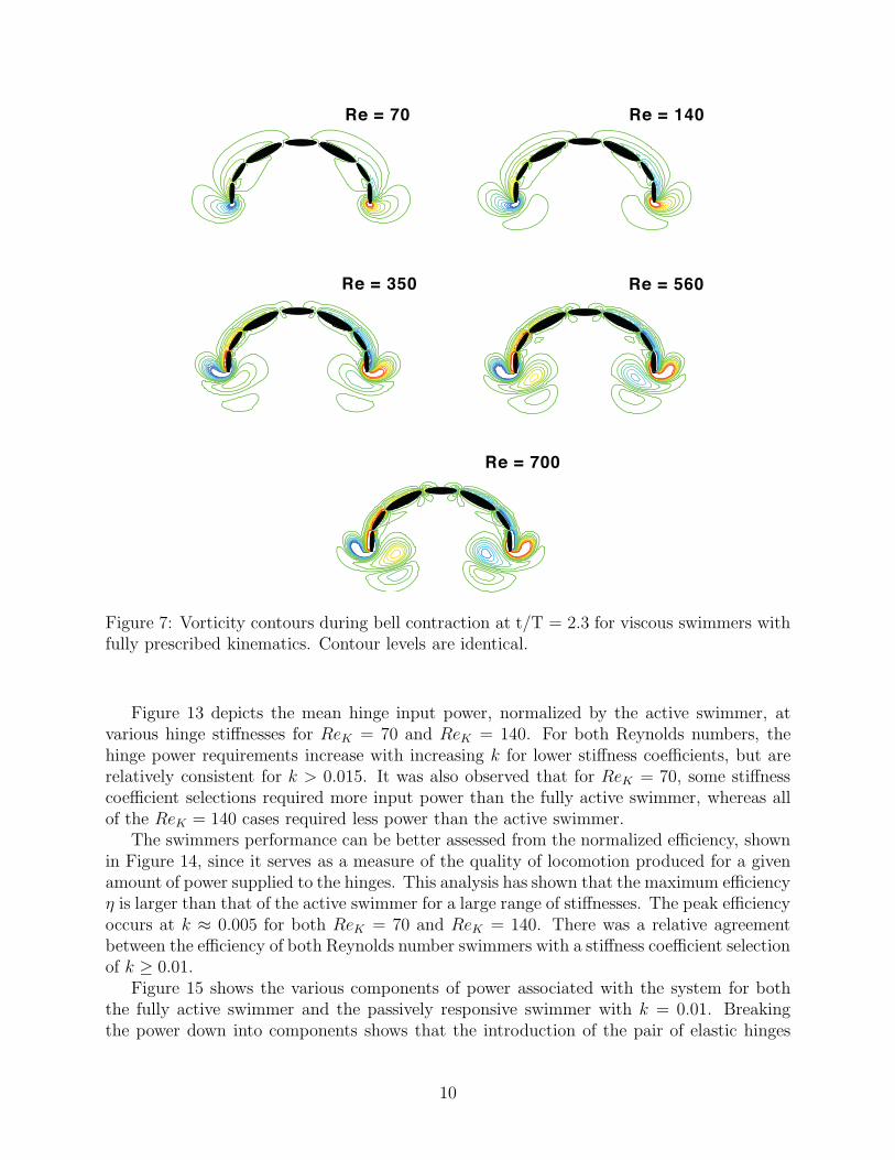
The instantaneous vorticity fields generated by the swimmers with fully prescribed kine-matics are shown at t/T = 2.3 in Figure 7 and exhibit traits that are consistent with previousexperimental studies of live oblate medusae swimming [13] and computational studies of sim-ilar models [21]. At the instant shown, the bell is in its contraction phase and a developingstarting vortex is attached to each lip of the orifice, accompanied just downstream in thewake by a fully-developed pair of stopping vortices. As ReK is increased, the rate at whichthe vortices diffuse in the wake is reduced, and a fully-developed starting vortex pair is stillpresent from the previous contraction cycle for several of the higher ReK cases. The strengthof the starting vortex pair still attached to the orifice lip increases with increasing Reynoldsnumber. Due to the nature of the Reynolds numbers in this investigation, the vorticity dif-fuses rapidly, prohibiting an extensive vortical wake from developing behind the swimmer,

8

0 100 200 300 400 500 600 700 800 900 10000

20

40

60

80

100

120

Reynolds Number

ωm

ax

Figure 6: Maximum value of vorticity based on ReK for t/T = 2.0 (), t/T = 2.3 (♦), andt/T = 2.6 (). Data for each t/T were fit with a corresponding quadratic polynomial ofnegative curvature.

unlike the aforementioned experimental and computational studies.

3.2 Peripheral hinges with passive kinematics

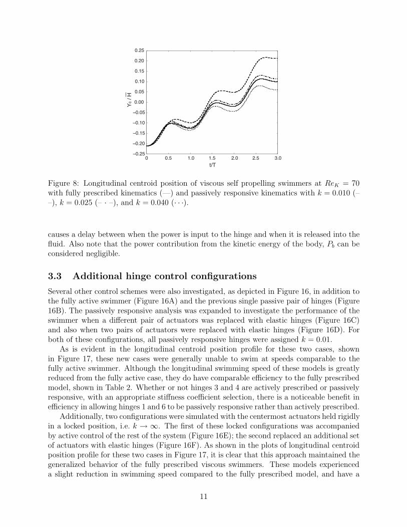
In this section, the fully active prescription of the kinematics is relaxed by replacing thehinges closest to the orifice lip (hinges 1 and 6) with elastic springs. As shown in Figure 8,the general behavior of the swimmer was largely unaffected. Some of the passive swimmersachieved a greater mean swimming speed than the fully prescribed case, shown in Figure 9,depending on the stiffness coefficient of the elastic hinge. The stiffness coefficient is definedas k = k∗/(ρfD

4max/T

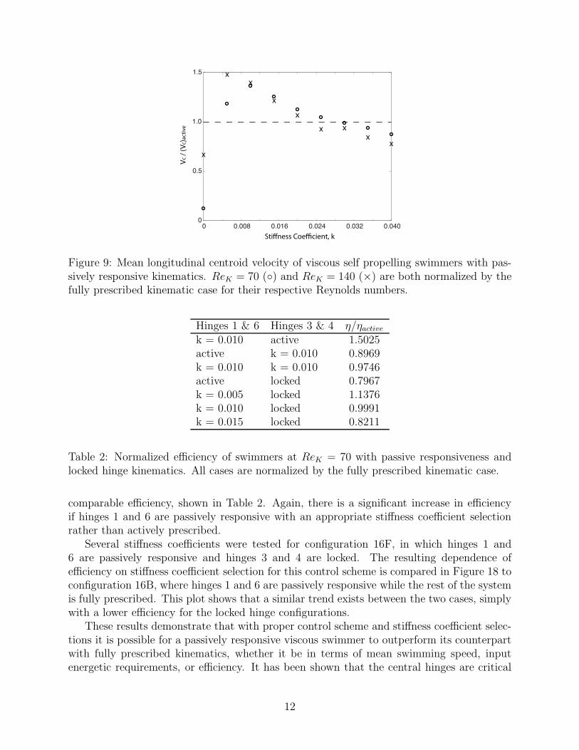
2), where k∗ is the dimensional stiffness. The swimming speed increasesrapidly with stiffness from k = 0 and exhibits a clear peak, at k = 0.010 for ReK = 70 andk ≈ 0.005 for ReK = 140. The mean speed decreases gradually with larger stiffness.

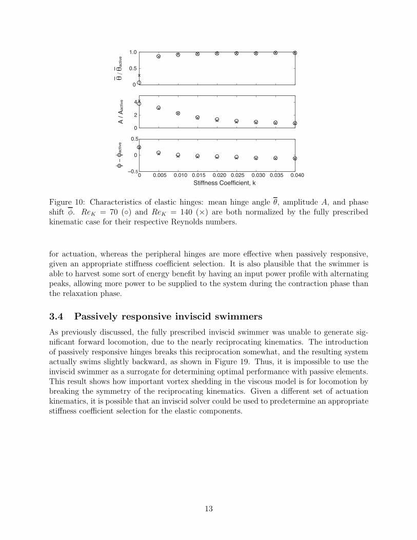
The response of the elastic hinge’s angular deflection is nearly sinusoidal, and can bedescribed by the mean hinge angle θ, the amplitude A, and the phase shift φ−φactive relativeto the fully active case, as shown in Figure 10. It is observed that at both ReK , while themean hinge angle and amplitude of the passively responsive case are tending towards thebehavior of the fully prescribed kinematics for k ≥ 0.02, there is a persistent discrepancy inthe phase shift from the active kinematics.

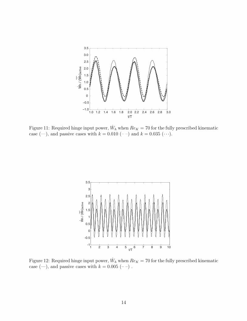
The required hinge input power signatures for the fully prescribed case and two passivecases are shown in Figure 11 for ReK = 70. The fully active case and the passive swimmerwith k = 0.010 have hinge input power peaks of alternating amplitude during the orificecontraction and and relaxation phases, the higher of which occurs during contraction. Thisis in contrast with the k = 0.035 swimmer, which has peaks of roughly equal amplitude.Figure 12 shows that the hinge input power signatures for two representative cases alsoremain constant on the longer time scale, 10T. This serves as further justification of usingthe shorter computation time 3T .

9

Re = 70 Re = 140

Re = 350 Re = 560

Re = 700

Figure 7: Vorticity contours during bell contraction at t/T = 2.3 for viscous swimmers withfully prescribed kinematics. Contour levels are identical.

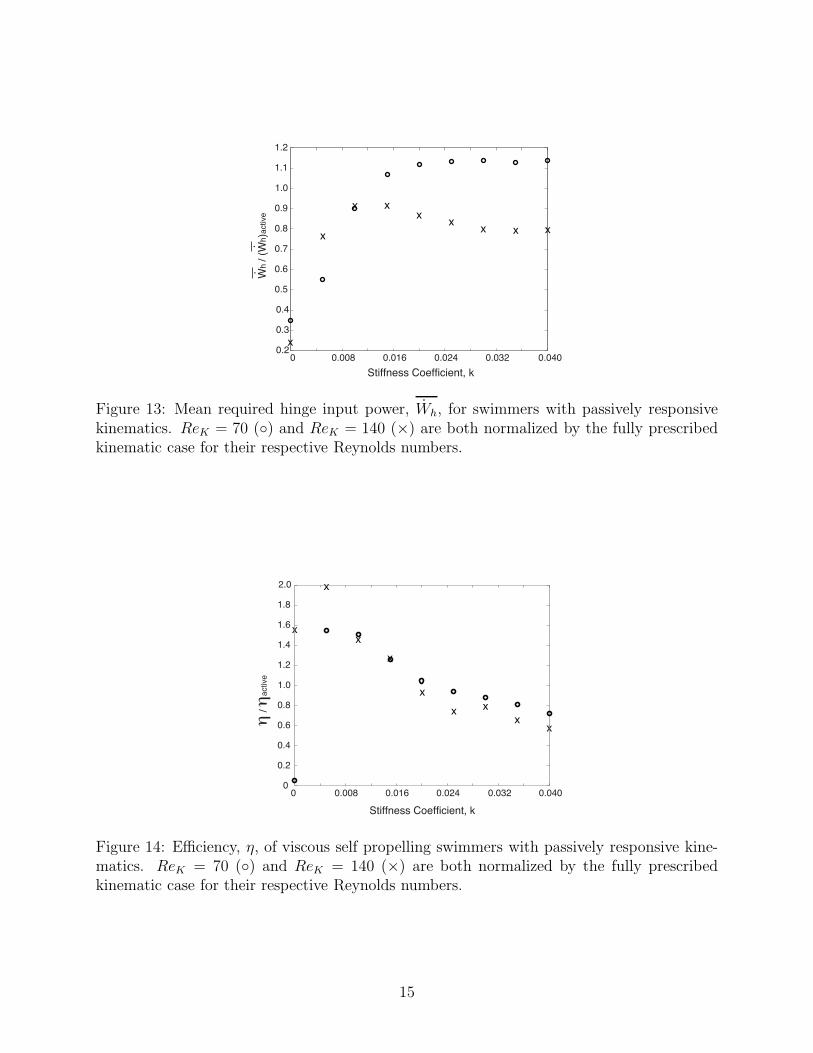
Figure 13 depicts the mean hinge input power, normalized by the active swimmer, atvarious hinge stiffnesses for ReK = 70 and ReK = 140. For both Reynolds numbers, thehinge power requirements increase with increasing k for lower stiffness coefficients, but arerelatively consistent for k > 0.015. It was also observed that for ReK = 70, some stiffnesscoefficient selections required more input power than the fully active swimmer, whereas allof the ReK = 140 cases required less power than the active swimmer.

The swimmers performance can be better assessed from the normalized efficiency, shownin Figure 14, since it serves as a measure of the quality of locomotion produced for a givenamount of power supplied to the hinges. This analysis has shown that the maximum efficiencyη is larger than that of the active swimmer for a large range of stiffnesses. The peak efficiencyoccurs at k ≈ 0.005 for both ReK = 70 and ReK = 140. There was a relative agreementbetween the efficiency of both Reynolds number swimmers with a stiffness coefficient selectionof k ≥ 0.01.

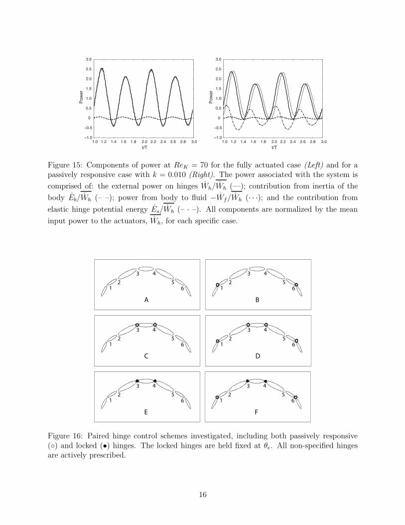
Figure 15 shows the various components of power associated with the system for boththe fully active swimmer and the passively responsive swimmer with k = 0.01. Breakingthe power down into components shows that the introduction of the pair of elastic hinges

10

0 0.5 1.0 1.5 2.0 2.5 3.0−0.25

−0.20

−0.15

−0.10

−0.05

0.00

0.05

0.10

0.15

0.20

0.25

t/T

Yc / H

Figure 8: Longitudinal centroid position of viscous self propelling swimmers at ReK = 70with fully prescribed kinematics (—) and passively responsive kinematics with k = 0.010 (––), k = 0.025 (– · –), and k = 0.040 (· · ·).

causes a delay between when the power is input to the hinge and when it is released into thefluid. Also note that the power contribution from the kinetic energy of the body, Pb can beconsidered negligible.

3.3 Additional hinge control configurations

Several other control schemes were also investigated, as depicted in Figure 16, in addition tothe fully active swimmer (Figure 16A) and the previous single passive pair of hinges (Figure16B). The passively responsive analysis was expanded to investigate the performance of theswimmer when a different pair of actuators was replaced with elastic hinges (Figure 16C)and also when two pairs of actuators were replaced with elastic hinges (Figure 16D). Forboth of these configurations, all passively responsive hinges were assigned k = 0.01.

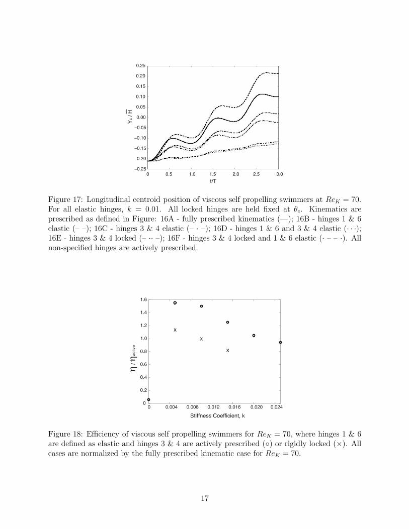
As is evident in the longitudinal centroid position profile for these two cases, shownin Figure 17, these new cases were generally unable to swim at speeds comparable to thefully active swimmer. Although the longitudinal swimming speed of these models is greatlyreduced from the fully active case, they do have comparable efficiency to the fully prescribedmodel, shown in Table 2. Whether or not hinges 3 and 4 are actively prescribed or passivelyresponsive, with an appropriate stiffness coefficient selection, there is a noticeable benefit inefficiency in allowing hinges 1 and 6 to be passively responsive rather than actively prescribed.

Additionally, two configurations were simulated with the centermost actuators held rigidlyin a locked position, i.e. k → ∞. The first of these locked configurations was accompaniedby active control of the rest of the system (Figure 16E); the second replaced an additional setof actuators with elastic hinges (Figure 16F). As shown in the plots of longitudinal centroidposition profile for these two cases in Figure 17, it is clear that this approach maintained thegeneralized behavior of the fully prescribed viscous swimmers. These models experienceda slight reduction in swimming speed compared to the fully prescribed model, and have a

11

0 0.008 0.016 0.024 0.032 0.0400

0.5

1.0

1.5

Stiness Coecient, k

Vc /

(V

c)a

cti

ve

x

x

xx

x

x

x x

x

Figure 9: Mean longitudinal centroid velocity of viscous self propelling swimmers with pas-sively responsive kinematics. ReK = 70 () and ReK = 140 (×) are both normalized by thefully prescribed kinematic case for their respective Reynolds numbers.

Hinges 1 & 6 Hinges 3 & 4 η/ηactive

k = 0.010 active 1.5025active k = 0.010 0.8969k = 0.010 k = 0.010 0.9746active locked 0.7967k = 0.005 locked 1.1376k = 0.010 locked 0.9991k = 0.015 locked 0.8211

Table 2: Normalized efficiency of swimmers at ReK = 70 with passive responsiveness andlocked hinge kinematics. All cases are normalized by the fully prescribed kinematic case.

comparable efficiency, shown in Table 2. Again, there is a significant increase in efficiencyif hinges 1 and 6 are passively responsive with an appropriate stiffness coefficient selectionrather than actively prescribed.

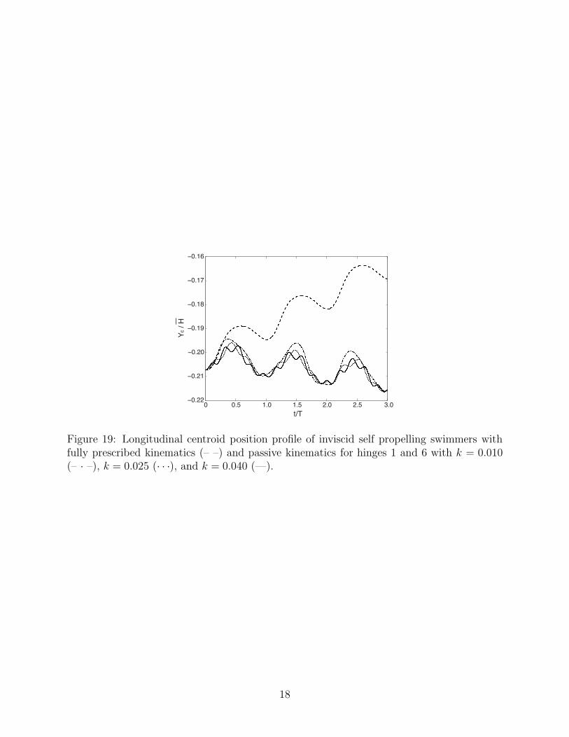
Several stiffness coefficients were tested for configuration 16F, in which hinges 1 and6 are passively responsive and hinges 3 and 4 are locked. The resulting dependence ofefficiency on stiffness coefficient selection for this control scheme is compared in Figure 18 toconfiguration 16B, where hinges 1 and 6 are passively responsive while the rest of the systemis fully prescribed. This plot shows that a similar trend exists between the two cases, simplywith a lower efficiency for the locked hinge configurations.

These results demonstrate that with proper control scheme and stiffness coefficient selec-tions it is possible for a passively responsive viscous swimmer to outperform its counterpartwith fully prescribed kinematics, whether it be in terms of mean swimming speed, inputenergetic requirements, or efficiency. It has been shown that the central hinges are critical

12

0

0.5

1.0

θ /

θactive

0

2

4

A / A

active

0 0.005 0.010 0.015 0.020 0.025 0.030 0.035 0.040−0.5

0

0.5

φ −

φa

ctive

Stiffness Coefficient, k

Figure 10: Characteristics of elastic hinges: mean hinge angle θ, amplitude A, and phaseshift φ. ReK = 70 () and ReK = 140 (×) are both normalized by the fully prescribedkinematic case for their respective Reynolds numbers.

for actuation, whereas the peripheral hinges are more effective when passively responsive,given an appropriate stiffness coefficient selection. It is also plausible that the swimmer isable to harvest some sort of energy benefit by having an input power profile with alternatingpeaks, allowing more power to be supplied to the system during the contraction phase thanthe relaxation phase.

3.4 Passively responsive inviscid swimmers

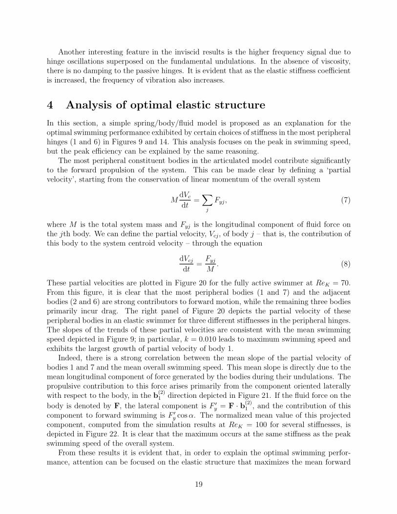
As previously discussed, the fully prescribed inviscid swimmer was unable to generate sig-nificant forward locomotion, due to the nearly reciprocating kinematics. The introductionof passively responsive hinges breaks this reciprocation somewhat, and the resulting systemactually swims slightly backward, as shown in Figure 19. Thus, it is impossible to use theinviscid swimmer as a surrogate for determining optimal performance with passive elements.This result shows how important vortex shedding in the viscous model is for locomotion bybreaking the symmetry of the reciprocating kinematics. Given a different set of actuationkinematics, it is possible that an inviscid solver could be used to predetermine an appropriatestiffness coefficient selection for the elastic components.

13

−1.0

−0.5

0

0.5

1.0

1.5

2.0

2.5

3.0

3.5

1.0 1.2 1.4 1.6 1.8 2.0 2.2 2.4 2.6 2.8 3.0

t/T

Wh / (

Wh)a

ctive

.

.

Figure 11: Required hinge input power, Wh when ReK = 70 for the fully prescribed kinematiccase (—), and passive cases with k = 0.010 (– –) and k = 0.035 (· · ·).

1 2 3 4 5 6 7 8 9 10-1

-0.5

0

0.5

1

1.5

2

2.5

3

3.5

t/T

Wh

/ (

Wh)a

ctive

..

__

Figure 12: Required hinge input power, Wh when ReK = 70 for the fully prescribed kinematiccase (—), and passive cases with k = 0.005 (– –) .

14

0 0.008 0.016 0.024 0.032 0.0400.2

0.3

0.4

0.5

0.6

0.7

0.8

0.9

1.0

1.1

1.2

Stiffness Coefficient, k

Wh

/ (

Wh)a

ctive

.

.

x

x

x

x xx

xx x

Figure 13: Mean required hinge input power, Wh, for swimmers with passively responsivekinematics. ReK = 70 () and ReK = 140 (×) are both normalized by the fully prescribedkinematic case for their respective Reynolds numbers.

xx

xx

x

x

x

x

x

0 0.008 0.016 0.024 0.032 0.0400

0.2

0.4

0.6

0.8

1.0

1.2

1.4

1.6

1.8

2.0

Stiffness Coefficient, k

η / η

active

Figure 14: Efficiency, η, of viscous self propelling swimmers with passively responsive kine-matics. ReK = 70 () and ReK = 140 (×) are both normalized by the fully prescribedkinematic case for their respective Reynolds numbers.

15

1.0 1.2 1.4 1.6 1.8 2.0 2.2 2.4 2.6 2.8 3.0

−1.0

−0.5

0

0.5

1.0

1.5

2.0

2.5

3.0

t/T

Power

1.0 1.2 1.4 1.6 1.8 2.0 2.2 2.4 2.6 2.8 3.0

−1.0

−0.5

0

0.5

1.0

1.5

2.0

2.5

3.0

t/T

Power

Figure 15: Components of power at ReK = 70 for the fully actuated case (Left) and for apassively responsive case with k = 0.010 (Right). The power associated with the system is

comprised of: the external power on hinges Wh/Wh (—); contribution from inertia of the

body Eb/Wh (– –); power from body to fluid −Wf/Wh (· · ·); and the contribution from

elastic hinge potential energy Es/Wh (– · –). All components are normalized by the mean

input power to the actuators, Wh, for each specific case.

1

2

3 4

5

6

A

1

2

3 4

5

6

B

1

2

3 4

5

6

C

1

2

3 4

5

6

D

1

2

3 4

5

6

E

1

2

3 4

5

6

F

Figure 16: Paired hinge control schemes investigated, including both passively responsive() and locked (•) hinges. The locked hinges are held fixed at θe. All non-specified hingesare actively prescribed.

16

0 0.5 1.0 1.5 2.0 2.5 3.0

−0.25

−0.20

−0.15

−0.10

−0.05

0.00

0.05

0.10

0.15

0.20

0.25

t/T

Yc / H

Figure 17: Longitudinal centroid position of viscous self propelling swimmers at ReK = 70.For all elastic hinges, k = 0.01. All locked hinges are held fixed at θe. Kinematics areprescribed as defined in Figure: 16A - fully prescribed kinematics (—); 16B - hinges 1 & 6elastic (– –); 16C - hinges 3 & 4 elastic (– · –); 16D - hinges 1 & 6 and 3 & 4 elastic (· · ·);16E - hinges 3 & 4 locked (– ·· –); 16F - hinges 3 & 4 locked and 1 & 6 elastic (· – – ·). Allnon-specified hinges are actively prescribed.

x

x

x

0 0.004 0.008 0.012 0.016 0.020 0.0240

0.2

0.4

0.6

0.8

1.0

1.2

1.4

1.6

Stiffness Coefficient, k

η / η

active

Figure 18: Efficiency of viscous self propelling swimmers for ReK = 70, where hinges 1 & 6are defined as elastic and hinges 3 & 4 are actively prescribed () or rigidly locked (×). Allcases are normalized by the fully prescribed kinematic case for ReK = 70.

17

0 0.5 1.0 1.5 2.0 2.5 3.0−0.22

−0.21

−0.20

−0.19

−0.18

−0.17

−0.16

t/T

Yc / H

Figure 19: Longitudinal centroid position profile of inviscid self propelling swimmers withfully prescribed kinematics (– –) and passive kinematics for hinges 1 and 6 with k = 0.010(– · –), k = 0.025 (· · ·), and k = 0.040 (—).

18

Another interesting feature in the inviscid results is the higher frequency signal due tohinge oscillations superposed on the fundamental undulations. In the absence of viscosity,there is no damping to the passive hinges. It is evident that as the elastic stiffness coefficientis increased, the frequency of vibration also increases.

4 Analysis of optimal elastic structure

In this section, a simple spring/body/fluid model is proposed as an explanation for theoptimal swimming performance exhibited by certain choices of stiffness in the most peripheralhinges (1 and 6) in Figures 9 and 14. This analysis focuses on the peak in swimming speed,but the peak efficiency can be explained by the same reasoning.

The most peripheral constituent bodies in the articulated model contribute significantlyto the forward propulsion of the system. This can be made clear by defining a ‘partialvelocity’, starting from the conservation of linear momentum of the overall system

MdVc

dt=

∑

j

Fyj , (7)

where M is the total system mass and Fyj is the longitudinal component of fluid force onthe jth body. We can define the partial velocity, Vcj, of body j – that is, the contribution ofthis body to the system centroid velocity – through the equation

dVcj

dt=

Fyj

M. (8)

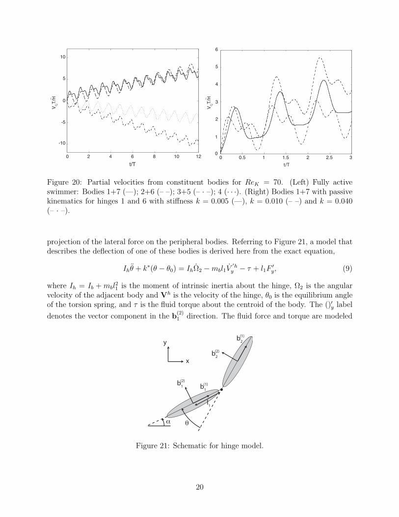
These partial velocities are plotted in Figure 20 for the fully active swimmer at ReK = 70.From this figure, it is clear that the most peripheral bodies (1 and 7) and the adjacentbodies (2 and 6) are strong contributors to forward motion, while the remaining three bodiesprimarily incur drag. The right panel of Figure 20 depicts the partial velocity of theseperipheral bodies in an elastic swimmer for three different stiffnesses in the peripheral hinges.The slopes of the trends of these partial velocities are consistent with the mean swimmingspeed depicted in Figure 9; in particular, k = 0.010 leads to maximum swimming speed andexhibits the largest growth of partial velocity of body 1.

Indeed, there is a strong correlation between the mean slope of the partial velocity ofbodies 1 and 7 and the mean overall swimming speed. This mean slope is directly due to themean longitudinal component of force generated by the bodies during their undulations. Thepropulsive contribution to this force arises primarily from the component oriented laterallywith respect to the body, in the b

(2)1 direction depicted in Figure 21. If the fluid force on the

body is denoted by F, the lateral component is F ′

y = F · b(2)1 , and the contribution of this

component to forward swimming is F ′

y cos α. The normalized mean value of this projectedcomponent, computed from the simulation results at ReK = 100 for several stiffnesses, isdepicted in Figure 22. It is clear that the maximum occurs at the same stiffness as the peakswimming speed of the overall system.

From these results it is evident that, in order to explain the optimal swimming perfor-mance, attention can be focused on the elastic structure that maximizes the mean forward

19

0 2 4 6 8 10 12

t/T

-10

-5

0

5

10V

CjT

/H_

0 0.5 1 1.5 2 2.5 3

t/T

5

4

3

2

1

0

6

VC

jT/H_

Figure 20: Partial velocities from constituent bodies for ReK = 70. (Left) Fully activeswimmer: Bodies 1+7 (—); 2+6 (– –); 3+5 (– · –); 4 (· · ·). (Right) Bodies 1+7 with passivekinematics for hinges 1 and 6 with stiffness k = 0.005 (—), k = 0.010 (– –) and k = 0.040(– · –).

projection of the lateral force on the peripheral bodies. Referring to Figure 21, a model thatdescribes the deflection of one of these bodies is derived here from the exact equation,

Ihθ + k∗(θ − θ0) = IhΩ2 − mbl1V′hy − τ + l1F

′

y, (9)

where Ih = Ib + mbl21 is the moment of intrinsic inertia about the hinge, Ω2 is the angular

velocity of the adjacent body and Vh is the velocity of the hinge, θ0 is the equilibrium angleof the torsion spring, and τ is the fluid torque about the centroid of the body. The ()′y label

denotes the vector component in the b(2)1 direction. The fluid force and torque are modeled

θα

b1

(1)b1

(2)

b2

(1)

b2

(2)

l1

x

y

Figure 21: Schematic for hinge model.

20

0

0

4

8

12

16

0.008 0.016 0.024 0.032 0.040

2F

’ yco

s α

/(M

H/T

2)

__________________

_

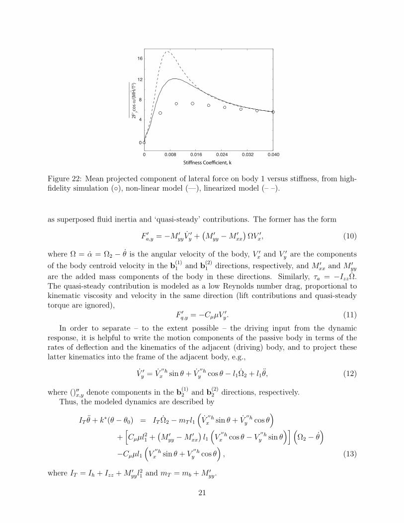
Figure 22: Mean projected component of lateral force on body 1 versus stiffness, from high-fidelity simulation (), non-linear model (—), linearized model (– –).

as superposed fluid inertia and ‘quasi-steady’ contributions. The former has the form

F ′

a,y = −M ′

yyV′

y +(

M ′

yy − M ′

xx

)

ΩV ′

x, (10)

where Ω = α = Ω2 − θ is the angular velocity of the body, V ′

x and V ′

y are the components

of the body centroid velocity in the b(1)1 and b

(2)1 directions, respectively, and M ′

xx and M ′

yy

are the added mass components of the body in these directions. Similarly, τa = −IzzΩ.The quasi-steady contribution is modeled as a low Reynolds number drag, proportional tokinematic viscosity and velocity in the same direction (lift contributions and quasi-steadytorque are ignored),

F ′

q,y = −CµµV ′

y . (11)

In order to separate – to the extent possible – the driving input from the dynamicresponse, it is helpful to write the motion components of the passive body in terms of therates of deflection and the kinematics of the adjacent (driving) body, and to project theselatter kinematics into the frame of the adjacent body, e.g.,

V ′

y = V′′hx sin θ + V

′′hy cos θ − l1Ω2 + l1θ, (12)

where ()′′x,y denote components in the b(1)2 and b

(2)2 directions, respectively.

Thus, the modeled dynamics are described by

IT θ + k∗(θ − θ0) = IT Ω2 − mT l1

(

V′′hx sin θ + V

′′hy cos θ

)

+[

Cµµl21 +(

M ′

yy − M ′

xx

)

l1

(

V′′hx cos θ − V

′′hy sin θ

)] (

Ω2 − θ)

−Cµµl1

(

V′′hx sin θ + V

′′hy cos θ

)

, (13)

where IT = Ih + Izz + M ′

yyl21 and mT = mb + M ′

yy.

21

For the kinematics imposed on the jellyfish system, the driving terms are well approxi-mated by sinusoidal functions,

V′′hx ≈ 0, V

′′hy ≈ −V h

1 sin(ω0t), Ω2 ≈ Ω21 sin(ω0t), (14)

where ω0 = 2π/T , V h1 = l1ω0 and Ω21 = 0.36ω0. The model equation is linearized for small

departures from equilibrium, θ = θ0 + θ(t), where |θ| ≪ 1. Furthermore, only terms varyingwith the fundamental frequency are retained. The resulting equation is

IT¨θ + Cµµl21

˙θ + k∗θ = D1 cos(ω0t) − D2 sin(ω0t) (15)

where D1 = ω0

(

IT Ω21 + mT l1Vh1 cos θ0

)

, D2 = −Cµµl1A and A = l1Ω21 + V h1 cos θ0. The

solution of this, ignoring start-up transients, is θ(t) = θ1 cos(ω0t + φ), where

θ1 =

[

D21 + D2

2

(k∗ − ω20IT )

2+ ω2

0C2µµ2l41

]1/2

, (16)

φ = arctan

(

−ω0Cµµl21k∗ − ω2

0IT

)

+ arctan(D2/D1). (17)

It is important (and unsurprising) to note that the peak hinge deflection occurs when k∗ =ω2

0IT .The linearized lateral force on the body is

F ′

y = −M ′

yyV′

y − CµµV ′

y . (18)

When this is projected in the swimming direction, with α = α2 − θ0 − Ω21/ω0 cos(ω0t) −θ1 cos(ω0t + φ). Here, α2, the mean angle of the adjacent body, is approximately 0.78, andθ0 = −0.72. The added mass of the elliptical body, accounting for the presence of theadjacent body, is determined empirically from the simulation results to be approximatelyM ′

yy = 2.4ρfπl21 and the resistive force coefficient is found to be Cµ ≈ 13.7; the addedmoment of inertia, Izz, is negligible. A comparison of the results for k = 0.04 between thefull simulation and this linearized model can be seen in Figure 23. The agreement is goodfor both the projected force and the hinge deflection.

The mean value of the projected lateral force can be computed analytically when theangle α is assumed to make only small perturbations about its mean value α2 − θ0. Theresulting expression can be written as

F ′

y cos α = −1

2sin(α2 − θ0)|F

′

y||α| cos(φF − φα), (19)

where F ′

y = |F ′

y| cos(ω0t + φF ) and α = |α| cos(ω0t + φα). This can be written as

F ′

y cos α =1

2sin(α2 − θ0)

[

M ′

yy

(

Ω221l1 + Ω21V

h1 cos θ0 + ω2

0l1θ21

)

+Fcθ1 cos φ − Fsθ1 sin φ] (20)

where Fc = ω0M′

yy(2Ω21l1 + V h1 cos θ0) and Fs = CµµV h

1 cos θ0.

22

20

15

10

5

0

0 0.5 1 1.5 2 2.5 3-5

25

t/T

2F

’ yco

s α

/(M

H/T

2)

_

0-0.9

-0.8

-0.7

-0.6

-0.5

-0.4

0.5 1 1.5 2 2.5 3

t/T

θ

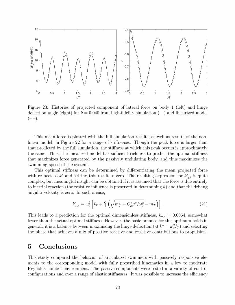
Figure 23: Histories of projected component of lateral force on body 1 (left) and hingedeflection angle (right) for k = 0.040 from high-fidelity simulation (—) and linearized model(– –).

This mean force is plotted with the full simulation results, as well as results of the non-linear model, in Figure 22 for a range of stiffnesses. Though the peak force is larger thanthat predicted by the full simulation, the stiffness at which this peak occurs is approximatelythe same. Thus, the linearized model has sufficient richness to predict the optimal stiffnessthat maximizes force generated by the passively undulating body, and thus maximizes theswimming speed of the system.

This optimal stiffness can be determined by differentiating the mean projected forcewith respect to k∗ and setting this result to zero. The resulting expression for k∗

opt is quitecomplex, but meaningful insight can be obtained if it is assumed that the force is due entirelyto inertial reaction (the resistive influence is preserved in determining θ) and that the drivingangular velocity is zero. In such a case,

k∗

opt = ω20

[

IT + l21

(√

m2T + C2

µµ2/ω2

0 − mT

)]

. (21)

This leads to a prediction for the optimal dimensionless stiffness, kopt = 0.0064, somewhatlower than the actual optimal stiffness. However, the basic premise for this optimum holds ingeneral: it is a balance between maximizing the hinge deflection (at k∗ = ω2

0IT ) and selectingthe phase that achieves a mix of positive reactive and resistive contributions to propulsion.

5 Conclusions

This study compared the behavior of articulated swimmers with passively responsive ele-ments to the corresponding model with fully prescribed kinematics in a low to moderateReynolds number environment. The passive components were tested in a variety of controlconfigurations and over a range of elastic stiffnesses. It was possible to increase the efficiency

23

of the system by replacing actuators with elastic springs; however this result was highly de-pendent on the configuration of the system and stiffness coefficient selection. Some of theseviscous swimmers were not only more effective but also were able to swim at a greater ratethan the fully actuated system. An inviscid solver was not found to be a useful surrogatefor this particular application due to the nearly reciprocating mechanics of the system. Thisresult emphasizes the importance of viscosity for breaking the symmetry of the kinematics.

A simple linear model was used to clarify the relationship between elastic structure andoptimal swimming performance. In particular, it was found that optimal performance iscorrelated to maximum mean fluid force generated by the undulating peripheral bodies. Fromthe model, an optimal stiffness was obtained that demonstrated that peak performance canbe obtained when the peripheral structure can achieve a balance between maximum deflectionresponse and a phasing that achieves a mix between reactive and resistive contributions.

From a biological standpoint, the muscular structure of hydromedusae only allow themto control the contraction phase during which water is expelled from the subumbrellar re-gion, generating thrust; during the relaxation phase, water is passively drawn back into thesubumbrellar region resulting from elastic strain energy stored during the previous part ofthe cycle [41]. Thus, intermediate future work would expand the current control scheme toallow the system to be actively controlled for the half-cycle during which contraction occurs,and passively thereafter. Allowing the relaxation phase to be entirely passive through use ofelastic strain energy could lead to reduced energy requirements of the system. Ultimately,the goal is to have an elastic three-dimensional single-body model with a more representa-tive fibrous structure, in contrast to the two-dimensional linked rigid body system used inthis analysis. However, the results obtained from this two-dimensional study can provideguidance for tailoring the elastic structure of the full body.

Acknowledgements

M. M. W. acknowledges the support of a GAANN Fellowship from the U.S. Departmentof Education. J. D. E. was supported by the National Science Foundation under awardCBET-0645228.

References

[1] A. J. Bergou, S. Xu, and Z. J. Wang. Passive wing pitch reversal in insect flight. Journalof Fluid Mechanics, 591:321–337, 2007.

[2] G. Berman and Z. J. Wang. Energy-minimizing kinematics in hovering insect flight.Journal of Fluid Mechanics, 582:153–168, 2007.

[3] J. D. Eldredge and J. Toomey. On the roles of chord-wise flexibility in a flapping wingwith hovering kinematics. Submitted to Journal of Fluid Mechanics, 2009.

[4] J. Toomey and J. D. Eldredge. Numerical and experimental study of the fluid dynamicsof a flapping wing with low order flexibility. Physics of Fluids, 20:073603–1–10, 2008.

24

[5] M. Vanella, T. Fitzgerald, S. Preidikman, E. Balaras, and B. Balachandran. Influence offlexibility on the aerodynamic performance of a hovering wing. Journal of ExperimentalBiology, 212:95–105, 2009.

[6] F. E. Fish and G. V. Lauder. Passive and active flow control by swimming fishes andmammals. Annual Review of Fluid Mechanics, 38:193–224, 2006.

[7] E. A. van Nierop, S. Alben, and M. P. Brener. How bumps on whale flippers delay stall:an aerodynamic model. Physical Review Letters, 100:054502, 2008.

[8] S. Alben, P. G. Madden, and G. V. Lauder. The mechanics of active fin-shape controlin ray-finned fishes. Journal of the Royal Society Interface, 4:243–256, 2007.

[9] R. McNeill Alexander. Tendon elasticity and muscle function. Comparative Biochemistryand Physiology - Part A: Molecular & Integrative Physiology, 133:1001 – 1011, 2002.

[10] F. E. Fish, M. K. Nusbaum, J. T. Beneski, and D. R. Ketten. Passive cambering andflexible propulsors: cetacean flukes. Bioinspiration and Biomimetics, 1:S42–S48, 2006.

[11] F. E. Fish, L. E. Howle, and M. M. Murray. Hydrodynamic flow control in marinemammals. Integrative and Comparative Biology, 48:788–800, 2008.

[12] M. D. Ford and J. H. Costello. Kinematic comparison of bell contraction by four speciesof hydromedusae. Scientia Marina, 64:47–53, 2000.

[13] J. O. Dabiri, S. P. Colin, J. H. Costello, and M. Gharib. Flow patterns generatedby oblate medusan jellyfish: field measurements and laboratory analyses. Journal ofExperimental Biology, 208:1257–1265, 2005.

[14] J. O. Dabiri, S. P. Colin, and J. H. Costello. Morphological diversity of medusan lineagesconstrained by animal-fluid interactions. Journal of Experimental Biology, 210:1868–1873, 2007.

[15] S. P. Colin and J. H. Costello. Morphology, swimming performance and propulsivemode of six co-occuring hydromedusae. Journal of Experimental Biology, 205:427–437,2002.

[16] M. J. McHenry and J. Jed. The ontogenetic scaling of hydrodynamics and swimmingperformance in jellyfish (Aurelia aurita). Journal of Experimental Biology, 206:4125–4137, 2003.

[17] J. Peng and J. O. Dabiri. Transport of inertial particles by Lagrangian coherent struc-tures: application to predator-prey interaction in jellyfish feeding. Journal of FluidMechanics, 623:75–84, 2009.

[18] J. Weston, S. P. Colin, J. H. Costello, and E. Abbott. Changing form and functionduring development in rowing hydromedusae. Marine Ecology-Progress Series, 374:127–134, 2009.

25

[19] M. M. Wilson, J. Peng, J. O. Dabiri, and J. D. Eldredge. Lagrangian coherent structuresin low Reynolds number swimming. Journal of Physics: Condensed Matter, 21:204105,2009.

[20] M. Sahin and K. Mohseni. An arbitrary Lagrangian–Eulerian formulation for the nu-merical simulation of flow patterns generated by the hydromedusa Aequorea victoria.Journal of Computational Physics, 228:4588–4605, 2009.

[21] M. Sahin, K. Mohseni, and S. P. Colin. The numerical comparison of flow patterns andpropulsive performances for the hydromedusae Sarsia tubulosa and Aequorea victoria.Journal of Experimental Biology, 212:2656–2667, 2009.

[22] D. Lipinski and K. Mohseni. Flow structures and fluid transport for the hydromedusaeSarsia tubulosa and Aequorea victoria. Journal of Experimental Biology, 212:2436–2447,2009.

[23] W. M. MeGill. The biomechanics of jellyfish swimming. PhD thesis, The University ofBritish Columbia, 2002.

[24] W. M. MeGill, J. .M. Gosline, and R. W. Blake. The modulus of elasticity of fibrillin-containing elastic fibres in the mesoglea of the hydromedusa Polyorchis penicillatus.Journal of Experimental Biology, 208:3819–3834, 2005.

[25] M. E. DeMont and J. M. Gosline. Mechanics of jet propulsion in the hydromedusanjellyfish, Polyorchis penicillatus, ii. energetics of the jet cycle. Journal of ExperimentalBiology, 134:333–345, 1988.

[26] D. A. Pabst. Springs in swimming animals. American Zoologist, 36:723–735, 1996.

[27] J. M. Gosline and R. E. Shadwick. The role of elastic energy storage mechanismsin swimming: an analysis of mantle elasticity in escape jetting in the squid, Loligoopalescens. Canadian Journal of Zoology, 61:1421–1431, 1983.

[28] S. Michelin, S. G. L. Smith, and B. J. Glover. Vortex shedding model of a flapping flag.Journal of Fluid Mechanics, 617:1–10, 2008.

[29] S. Alben. Optimal flexibility of a flapping appendage in an inviscid fluid. Journal ofFluid Mechanics, 614:355–380, 2008.

[30] S. Alben, M. J. Shelley, and J. Zhang. Drag reduction through self-similar bending ofa flexible body. Nature, 420:479–481, 2002.

[31] S. Alben, M. J. Shelley, and J. Zhang. How flexibility induces streamlining in a two-dimensional flow. Physics of Fluids, 16:1694–1713, 2004.

[32] M. J. McHenry. Comparative biomechanics: The jellyfish paradox resolved. CurrentBiology, 17:R632–R633, 2007.

[33] J. D. Eldredge. Dynamically coupled fluid-body interaction in vorticity-based numericalsimulations. Journal of Computational Physics, 227:9170–9194, 2008.

26

[34] J. Peng and J. O. Dabiri. A potential-flow, deformable-body model for fluid-structureinteractions with compact vorticity: application to animal swimming measurements.Experiments in Fluids, 43:655–664, Nov 2007.

[35] E. Kanso, J. E. Marsden, C. W. Rowley, and J. Melli-Huber. Locomotion of articulatedbodies in a perfect fluid. Journal of Nonlinear Science, 15:255–289, 2005.

[36] S. D. Kelly. The mechanics and control of robotic locomotion with applications toaquatic vehicles. PhD thesis, California Institute of Technology, 1998.

[37] J. D. Eldredge. Numerical simulations of undulatory swimming at moderate Reynoldsnumber. Bioinspiration and Biomimetics, 1:S19–S24, 2006.

[38] E. M. Purcell. Life at low Reynolds number. American Journal of Physics, 45:3–11,1977.

[39] J. D. Eldredge. Numerical simulation of the fluid dynamics of 2D rigid body motionwith the vortex particle method. Journal of Computational Physics, 221:626–648, 2007.

[40] S. Childress. Mechanics of swimming and flying. Cambridge University Press, 1984.

[41] T. L. Daniel. Cost of locomotion: unsteady medusan swimming. Journal of Experimen-tal Biology, 119:149–164, 1985.

27