47
Performance Performance Measurement Measurement
| Date post: | 02-Jan-2016 |
| Category: |
Documents |
| Upload: | annis-marsh |
| View: | 214 times |
| Download: | 1 times |

Performance MeasurementPerformance Measurement

A Quantitative Basis for DesignA Quantitative Basis for Design
Parallel programming is an optimization Parallel programming is an optimization problem.problem.
Must take into account several factors:Must take into account several factors:– execution timeexecution time– scalabilityscalability– efficiencyefficiency

A Quantitative Basis for DesignA Quantitative Basis for Design
Parallel programming is an optimization Parallel programming is an optimization problem.problem.
Must take into account several factors:Must take into account several factors: Also must take into account the costs:Also must take into account the costs:
– memory requirementsmemory requirements– implementation costsimplementation costs– maintenance costs etc.maintenance costs etc.

A Quantitative Basis for DesignA Quantitative Basis for Design
Parallel programming is an optimization Parallel programming is an optimization problem.problem.
Must take into account several factors:Must take into account several factors: Also must take into account the costs:Also must take into account the costs: Mathematical performance models are used Mathematical performance models are used
to assess these costs and predict to assess these costs and predict performance.performance.
Defining PerformanceDefining Performance
How do you define parallel performance?How do you define parallel performance? What do you define it in terms of?What do you define it in terms of? ConsiderConsider
– Distributed databasesDistributed databases– Image processing pipelineImage processing pipeline– Nuclear weapons testbedNuclear weapons testbed

Metrics for PerformanceMetrics for Performance
EfficiencyEfficiency SpeedupSpeedup ScalabilityScalability Others …………..Others …………..

Some TermsSome Terms
s(n,p) = speedup for problem size n on p processorss(n,p) = speedup for problem size n on p processors o(n) = serial portion of computationo(n) = serial portion of computation p(n) = parallel portion of computationp(n) = parallel portion of computation c(n,p) = time for communicationc(n,p) = time for communication Speed1 = o(n) + p(n)Speed1 = o(n) + p(n) SpeedP = o(n) + p(n)/p + c(n,p)SpeedP = o(n) + p(n)/p + c(n,p)

EfficiencyEfficiency
pTp
T1E The fraction of time a processor spends doing useful work
What about when pTWhat about when pTpp < T < T11
– Does cache make a processor work at 110%?Does cache make a processor work at 110%?
o(n) + p(n)
p * o(n) + p(n) + p * c(n,p)E =

SpeedupSpeedup
SpeedP
SpeedS
1
What is Speed?
What algorithm for Speed1?
What is the work performed?How much work?

Speedup (More Detail)Speedup (More Detail)
s(n,p) = speedup for problem size n on p processorss(n,p) = speedup for problem size n on p processors o(n) = serial portion of computationo(n) = serial portion of computation p(n) = parallel portion of computationp(n) = parallel portion of computation c(n,p) = time for communicationc(n,p) = time for communication Speed1 = o(n) + p(n)Speed1 = o(n) + p(n) SpeedP = o(n) + p(n)/p + c(n,p)SpeedP = o(n) + p(n)/p + c(n,p)
o(n) + p(n)
o(n) + p(n)/p + c(n,p)Speedup =

More on SpeedupMore on Speedup
Computation time decreases as we add processors butcommunication time increases

Two kinds of SpeedupTwo kinds of Speedup
RelativeRelative– Uses parallel algorithm on 1 processorUses parallel algorithm on 1 processor– Most commonMost common– Useful for determining algorithm scalabilityUseful for determining algorithm scalability
AbsoluteAbsolute– Uses best known serial algorithmUses best known serial algorithm– Eliminates overheads in calculation.Eliminates overheads in calculation.– Useful to express absolute performanceUseful to express absolute performance
Story: Prime Number GenerationStory: Prime Number Generation

Amdahl's LawAmdahl's Law
Every algorithm has a sequential component.Every algorithm has a sequential component. Sequential component limits speedupSequential component limits speedup
SequentialComponent
MaximumSpeedup
= 1/s = s
¾ can be parallelized ¼ sequential¼ sequential
Suppose each ¼ of the program takes 1 unit of timeSpeedup = 1 proc time / n proc time = 4/1 = 4

AmdahlAmdahl’’s Laws Law
o(n) + p(n)
o(n) + p(n)/p + c(n,p)Speedup =
o(n) + p(n)
o(n) + p(n)/p <=
s = o(n)/(o(n) + p(n)) = the inherently sequential percentage
Speedup <=o(n) / s
o(n) + o(n) ( 1/s -1)/p
Speedup <=1
s + ( 1 - s)/p

Amdahl's LawAmdahl's Law
s
Speedup

SpeedupSpeedup
Algorithm AAlgorithm A– Serial execution time is 10 sec.Serial execution time is 10 sec.– Parallel execution time is 2 sec.Parallel execution time is 2 sec.
Algorithm BAlgorithm B– Serial execution time is 2 sec.Serial execution time is 2 sec.– Parallel execution time is 1 sec.Parallel execution time is 1 sec.
What if I told you A = B?What if I told you A = B?


SpeedupSpeedup
Conventional speedup is defined as the Conventional speedup is defined as the reduction in execution time.reduction in execution time.
Consider running a problem on a slow Consider running a problem on a slow parallel computer and on a faster one.parallel computer and on a faster one.– Same serial componentSame serial component– Speedup will be lower on the faster computer.Speedup will be lower on the faster computer.

LogicLogic
The art of thinking and reasoning in strict The art of thinking and reasoning in strict accordance with the limitations and accordance with the limitations and incapacities of the human misunderstanding. incapacities of the human misunderstanding.
The basis of logic is the syllogism, The basis of logic is the syllogism, consisting of a major and minor premise and consisting of a major and minor premise and a conclusion.a conclusion.

ExampleExample
Major Premise: Sixty men can do a piece of Major Premise: Sixty men can do a piece of work sixty times as quickly as one man.work sixty times as quickly as one man.
Minor Premise: One man can dig a post-Minor Premise: One man can dig a post-hole in sixty seconds.hole in sixty seconds.
Conclusion: Sixty men can dig a post-hole Conclusion: Sixty men can dig a post-hole in one second.in one second.

Speedup and Amdahl's LawSpeedup and Amdahl's Law
Conventional speedup Conventional speedup penalizes penalizes faster faster absolute speed.absolute speed.
Assumption that task size is constant as the Assumption that task size is constant as the computing power increases results in an computing power increases results in an exaggeration of task overhead.exaggeration of task overhead.
Scaling the problem size reduces these Scaling the problem size reduces these distortion effects.distortion effects.

SolutionSolution
Gustafson introduced scaled speedup.Gustafson introduced scaled speedup. Scale the problem size as you increase the Scale the problem size as you increase the
number of processors.number of processors. Calculated in two waysCalculated in two ways
– ExperimentallyExperimentally– Analytical modelsAnalytical models

Traditional SpeedupTraditional Speedup(Strong Scaling)(Strong Scaling)
)(
)(1
NT
NTSpeedup
P
Tx (y) is time taken to solve problem ofsize y on x processors
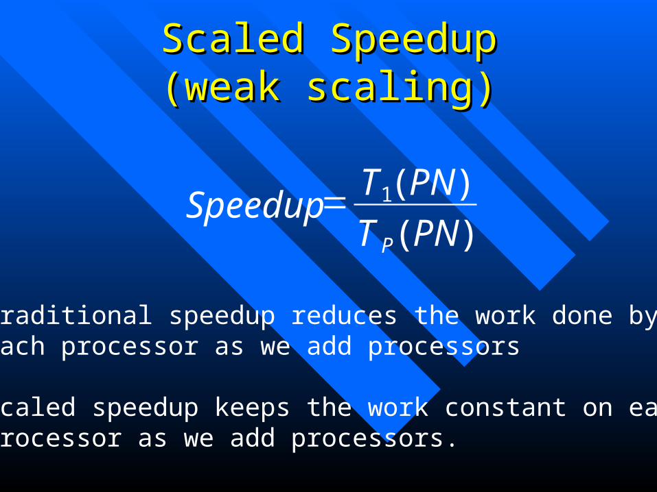
Scaled SpeedupScaled Speedup(weak scaling)(weak scaling)
)(
)(1
PNT
PNTSpeedup
P
Traditional speedup reduces the work done byeach processor as we add processors
Scaled speedup keeps the work constant on eachprocessor as we add processors.

Scaled SpeedupScaled Speedupo(n) + p(n)
o(n) + p(n)/p Speedup <=
can be divided into two piecesserial and parallel
s = o(n) / (o(n) + p(n)/p) and (1 – s) = p(n)/p / (o(n) + p(n)/p)now solve for o(n) and p(n) respectively
o(n) = (o(n) + p(n)/p) * sp(n) = (o(n) + p(n)/p) * (1 – s) * p
substituting these back into Speedup Equation yeildsSpeedup <= s + (1 – s) * p and Speedup <= p + (1 – p) * s
where s is fraction of time doing serial code = o(n) / t(n,k)t(n,k) is time of parallel program for size n on k processors
Thus, max speedup with p < k processors isSpeedup <= p + (1 – p) * s

Traditional SpeedupTraditional Speedup
ideal
measured
Number of Processors
Speedup

Scaled SpeedupScaled Speedup
ideal
Number of Processors
Speedup
Small problem
Medium problem
Large Problem

Scaled Speedup vs AmdahlScaled Speedup vs Amdahl’’s Laws Law
AmdahlAmdahl’’s Law determines speedup by taking a serial s Law determines speedup by taking a serial computation and predicting how quickly it could be done computation and predicting how quickly it could be done in parallelin parallel
Scaled speedup begins with a parallel computation and Scaled speedup begins with a parallel computation and estimates how much faster the parallel computation is than estimates how much faster the parallel computation is than the same computation on a serial processorthe same computation on a serial processor
strong scalingstrong scaling is defined as how the solution time varies is defined as how the solution time varies with the number of processors for a fixed with the number of processors for a fixed totaltotal problem problem size.size.
weak scalingweak scaling is defined as how the solution time varies is defined as how the solution time varies with the number of processors for a fixed problem size with the number of processors for a fixed problem size per per processorprocessor..

Determining Scaled SpeedupDetermining Scaled Speedup
Time problem size n on 1 processorTime problem size n on 1 processor Time problem size 2n on 2 processorsTime problem size 2n on 2 processors Time problem size 2n on 1 processorTime problem size 2n on 1 processor Time problem size 4n on 4 processorsTime problem size 4n on 4 processors Time problem size 4n on 1 processorTime problem size 4n on 1 processor etc.etc. Plot the curvePlot the curve

Performance MeasurementPerformance Measurement
There is not a perfect way to measure and There is not a perfect way to measure and report performance.report performance.
Wall clock time seems to be the best.Wall clock time seems to be the best. But how much work do you do?But how much work do you do? Best Bet:Best Bet:
– Develop a model that fits experimental results.Develop a model that fits experimental results.

A Parallel Programming ModelA Parallel Programming Model
Goal: Define an equation that predicts Goal: Define an equation that predicts execution time as a function of execution time as a function of – Problem sizeProblem size– Number of processorsNumber of processors– Number of tasksNumber of tasks– Etc.Etc.
,....),( PNfT

A Parallel Programming ModelA Parallel Programming Model
Execution time can be broken up into Execution time can be broken up into – ComputingComputing– CommunicatingCommunicating– IdlingIdling
idlecommcomp TTTT

Computation TimeComputation Time
Normally depends on problem sizeNormally depends on problem size Also depends on machine characteristicsAlso depends on machine characteristics
– Processor speedProcessor speed– Memory systemMemory system– Etc.Etc.
Often, experimentally obtainedOften, experimentally obtained

Communication TimeCommunication Time
The amount of time spent sending & The amount of time spent sending & receiving messagesreceiving messages
Most often is calculated as Most often is calculated as – Cost of sending a single message * #messagesCost of sending a single message * #messages
Single message costSingle message cost– T = startuptime + T = startuptime +
time_to_send_one_word * #words time_to_send_one_word * #words

Idle TimeIdle Time
Difficult to determineDifficult to determine This is often the time waiting for a message This is often the time waiting for a message
to be sent to you.to be sent to you. Can be avoided by overlapping Can be avoided by overlapping
communication and computation.communication and computation.

Finite Difference ExampleFinite Difference Example
Finite Difference CodeFinite Difference Code 512 x 512 x 5 Elements512 x 512 x 5 Elements
Nine-point stencilNine-point stencil Row-wise decompositionRow-wise decomposition
– Each processor gets n/p*n*z elementsEach processor gets n/p*n*z elements
16 IBM RS6000 workstations16 IBM RS6000 workstations Connected via EthernetConnected via Ethernet
z n xn x

Finite Difference ModelFinite Difference Model
Execution Time (per iteration)Execution Time (per iteration)– ExTime = (Tcomp + Tcomm)/PExTime = (Tcomp + Tcomm)/P
Communication Time (per iteration)Communication Time (per iteration)– Tcomm = 2 (lat + 2*n*z*bw)Tcomm = 2 (lat + 2*n*z*bw)
Computation TimeComputation Time– Estimate using some sample codeEstimate using some sample code

Estimated PerformanceEstimated Performance

Finite Difference ExampleFinite Difference Example

What was wrong?What was wrong?
EthernetEthernet– Shared busShared bus
Change the computation of TcommChange the computation of Tcomm– Reduce the bandwithReduce the bandwith– Scale the message volume by the number of Scale the message volume by the number of
processors sending concurrently.processors sending concurrently.– Tcomm = 2 (lat + 2*n*z*bw * P/2)Tcomm = 2 (lat + 2*n*z*bw * P/2)

Finite Difference ExampleFinite Difference Example
Using analytical modelsUsing analytical models
Examine the control flow of the algorithmExamine the control flow of the algorithm Find a general algebraic form for the Find a general algebraic form for the
complexity (execution time).complexity (execution time). Fit the curve with experimental data.Fit the curve with experimental data. If the fit is poor, find the missing terms and If the fit is poor, find the missing terms and
repeat.repeat. Calculate the scaled speedup using formula.Calculate the scaled speedup using formula.

ExampleExample
Serial Time = 2 + 12 N secondsSerial Time = 2 + 12 N seconds Parallel Time = 4 + 12 N/P + 5P secondsParallel Time = 4 + 12 N/P + 5P seconds Let N/P = 128Let N/P = 128 Scaled Speedup for 4 processors is:Scaled Speedup for 4 processors is:
93.31560
6146)4(5)4/)128(4(124
))128(4(122
)(
)(1 PNC
PNC
P

Performance EvaluationPerformance Evaluation
Identify the dataIdentify the data Design the experiments to obtain the dataDesign the experiments to obtain the data Report dataReport data

Performance EvaluationPerformance Evaluation
Identify the dataIdentify the data– Execution timeExecution time– Be sure to examine a range of data pointsBe sure to examine a range of data points
Design the experiments to obtain the dataDesign the experiments to obtain the data Report dataReport data

Performance EvaluationPerformance Evaluation
Identify the dataIdentify the data Design the experiments to obtain the dataDesign the experiments to obtain the data
– Make sure the experiment measures what you Make sure the experiment measures what you intend to measure.intend to measure.
– Remember: Execution time is max time taken.Remember: Execution time is max time taken.– Repeat your experiments many timesRepeat your experiments many times– Validate data by designing a modelValidate data by designing a model
Report dataReport data

Performance EvaluationPerformance Evaluation
Identify the dataIdentify the data Design the experiments to obtain the dataDesign the experiments to obtain the data Report dataReport data
– Report all information that affects executionReport all information that affects execution– Results should be separate from ConclusionsResults should be separate from Conclusions– Present the data in an easily understandable Present the data in an easily understandable
format.format.


