Helsinki University of Technology Networking Laboratory Teknillinen korkeakoulu Tietoverkkolaboratorio Espoo 2006 Report 3/2006 PERFORMANCE STUDIES OF WIRELESS MULTIHOP NETWORKS Henri Koskinen Dissertation for the degree of Doctor of Science in Technology to be presented with due permission for public examination and debate in Auditorium S4 at Helsinki University of Technology (Espoo, Finland) on the 12th of May, 2006, at 12 o’clock noon. Helsinki University of Technology Department of Electrical and Communications Engineering Networking Laboratory Teknillinen korkeakoulu S¨ ahk ¨ o- ja tietoliikennetekniikan osasto Tietoverkkolaboratorio
Transcript
Helsinki University of Technology Networking LaboratoryTeknillinen korkeakoulu Tietoverkkolaboratorio
Espoo 2006 Report 3/2006
PERFORMANCE STUDIES OF WIRELESS MULTIHOP
NETWORKS
Henri Koskinen
Dissertation for the degree of Doctor of Science in Technology to be presented with duepermission for public examination and debate in Auditorium S4 at Helsinki University ofTechnology (Espoo, Finland) on the 12th of May, 2006, at 12 o’clock noon.
Helsinki University of Technology
Department of Electrical and Communications Engineering
HELSINKI UNIVERSITY OF TECHNOLOGY ABSTRACT OF DOCTORAL DISSERTATIONP.O.BOX 1000, FIN-02015 TKKhttp://www.tkk.fi/
Author: Henri KoskinenName of the dissertationPerformance Studies of Wireless Multihop NetworksDate of manuscript 5th of December 2005 Date of the dissertation 12th of May 2006
Monograph × Article dissertation (summary + original articles)Department Department of Electrical and Communications EngineeringLaboratory Networking LaboratoryField of Research Teletraffic TheoryOpponent Professor Patrick Thiran (Ecole Polytechnique Federale de Lausanne, Switzerland)Supervisor Professor Jorma Virtamo (Helsinki University of Technology)Abstract
Wireless multihop networks represent a fundamental step in the evolution of wireless communications, a step thathas proven challenging. Such networks give rise to a wide range of novel performance and design problems, most ofwhich are of a geometric nature. This dissertation addresses a selection of such problems.
The first part of this thesis presents studies in which the network nodes are assumed to receive signals sufficientlyclearly only from within some fixed range of operation. Using this simple model, the first two problems addressedare to predict the probabilities that a network with randomly placed nodes is connected or completely covers agiven target domain, respectively. These problems are equivalent to determining the probability distribution of theminimal range providing connectivity or coverage. Algorithms for determining these threshold ranges for a given setof network nodes are developed. Because of the complex nature of these problems in finite settings, they are bothapproached by empirically modeling the convergence of these distributions to their known asymptotic limits. Next, anovel optimization problem is presented, in which the task is to make a given disconnected network into a connectedone by adding a minimal number of additional nodes to the network, and heuristic algorithms are proposed for thisproblem.
In the second part, these networks are studied in the context of a more realistic model in which the condition forsuccessful communication between network nodes is expressed as an explicit minimum value for the received signal-to-noise-and-interference ratio. The notion of the threshold range for connectivity is first generalized to this networkmodel. Because connectivity is now affected by medium access control (MAC), two alternative MAC schemes areconsidered. Finally, an infinite random network employing slotted Aloha is studied under this model. Since theprobability of successful reception in a random time slot is a function of the locations of other nodes, this temporalprobability is a random variable with its own probability distribution over different node configurations. Numericalapproximations for evaluating both the mean and the tail probability of this distribution are developed. The accuracyof these approximations can be improved indefinitely, at the cost of numerical computations.
Keywords wireless multihop networks, ad hoc networks, sensor networks, connectivity, coverage,throughput, geometric random graphs, stochastic geometry
ISBN (printed) 951-22-8136-8 ISSN (printed) 1458-0322ISBN (pdf) 951-22-8137-6 ISSN (pdf)ISBN (others) Number of pages 84 p. + app. 84 p.Publisher Networking Laboratory / Helsinki University of TechnologyPrint distribution× The dissertation can be read at http://lib.tkk.fi/Diss/
Tekija: Henri KoskinenVaitoskirjan nimiTutkimuksia langattomien monihyppyisten verkkojen suorituskyvystaKasikirjoituksen jattamispaivamaara 5. joulukuuta 2005 Vaitostilaisuuden paivamaara 12. toukokuuta 2006
Monografia × Yhdistelmavaitoskirja (yhteenveto + erillisartikkelit)Osasto Sahko- ja tietoliikennetekniikan osastoLaboratorio TietoverkkolaboratorioTutkimusala TeleliikenneteoriaVastavaittaja Professori Patrick Thiran (Ecole Polytechnique Federale de Lausanne, Sveitsi)Tyon valvoja Professori Jorma Virtamo (Teknillinen korkeakoulu)Tiivistelma
Langattomat monihyppyiset verkot edustavat langattoman viestinnan perustavanlaatuista kehitysaskelta, joka on osoit-tautunut haasteelliseksi. Tallaisissa verkoissa tulee esiin monenlaisia uusia suorituskyky- ja suunnitteluongelmia,joista useimmat ovat luonteeltaan geometrisia. Tassa vaitoskirjassa kasitellaan joitakin tallaisia ongelmia.
Tyon ensimmainen osa esittelee tutkimuksia, joissa verkon solmujen oletetaan vastaanottavan signaaleja riittavanvoimakkaina vain tietyn kiintean toimintakantaman sisalta. Taman yksinkertaisen mallin puitteissa kaksi en-simmaista tarkasteltavaa ongelmaa ovat ennustaa todennakoisyydet sille, etta satunnaisesti sijaitsevien solmujen muo-dostama verkko on yhtenainen ja toisaalta taysin peittaa annetun kohdealueen. Naiden kanssa ekvivalentit ongel-mat on maarittaa yhtenaisyyden tai tayden peiton tuovan pienimman kantaman todennakoisyysjakauma. Tyossa ke-hitetaan algoritmeja, joilla nama kynnyskantamat maaritetaan annetulle solmujoukolle. Koska ongelmat ovat luon-teeltaan monimutkaisia aarellisissa tapauksissa, lahestytaan kumpaakin mallintamalla empiirisesti naiden jakaumiensuppenemista kohti tunnettuja asymptoottisia rajajakaumiaan. Seuraavaksi esitetaan uusi optimointiongelma, jossatehtavana on tehda annetusta epayhtenaisesta verkosta yhtenainen sijoittamalla verkkoon mahdollisimman vahanlisasolmuja, ja kehitetaan ongelmaan heuristisia algoritmeja.
Toisessa osassa naita verkkoja tutkitaan kayttaen realistisempaa mallia, jossa verkon solmujen valisen viestinnan on-nistumisehto ilmaistaan vastaanotetun signaali-hairiosuhteen minimiarvona. Aluksi yleistetaan verkon yhtenaisyy-den kynnyskantaman kasite tahan verkkomalliin. Koska verkon yhtenaisyyteen vaikuttaa nyt solmujen lahetyskuri(medium access control; MAC), tarkastellaan kahta vaihtoehtoista MAC-protokollaa. Lopuksi tutkitaan aaretonta sa-tunnaista, aikajaettua Aloha-satunnaisliityntaa kayttavaa verkkoa taman mallin puitteissa. Koska lahetyksen vastaan-oton onnistumistodennakoisyys satunnaisessa aikavalissa on muiden solmujen sijaintien funktio, tama ajallinen to-dennakoisyys on satunnaismuuttuja, jolla on oma todennakoisyysjakaumansa yli erilaisten solmukonfiguraatioiden.Taman jakauman odotusarvon ja hantatodennakoisyyden arvioimiseksi kehitetaan numeerisia approksimaatioita,joiden tarkkuutta voidaan parantaa rajatta, numeerisen laskentatyon kustannuksella.
ISBN (painettu) 951-22-8136-8 ISSN (painettu) 1458-0322ISBN (pdf) 951-22-8137-6 ISSN (pdf)ISBN (muut) Sivumaara 84 s. + liit. 84 s.Julkaisija Tietoverkkolaboratorio / Teknillinen korkeakouluPainetun vaitoskirjan jakelu× Luettavissa verkossa osoitteessa http://lib.tkk.fi/Diss/
PREFACE
This dissertation is the result of research that began in 2002, when I startedto work on my Master’s Thesis in the Networking Laboratory of HelsinkiUniversity of Technology. The work has been carried out in the AHRASproject, funded by the Finnish Defence Forces Technical Research Centre,as well as in the NAPS project funded by the Academy of Finland. In2004, I was granted the honor of being admitted to the Graduate Schoolof Electronics, Telecommunications and Automation (GETA), which hassince provided the majority of the funding. In addition, personal financialsupport from the TES and Nokia foundations is gratefully acknowledged.
I wish to express my gratitude to my supervisor, Professor Jorma Vir-tamo, for the privilege of receiving his guidance throughout my work. Hissolid expertise in research never ceases to impress me. I also thank Drs. EsaHyytia, Jouni Karvo, and Pasi Lassila, as well as M.Sc. Olli Apilo, for theirwork as co-authors of the publications, and the pre-examiners of this disser-tation, Professor Christian Bettstetter and Dr. Bartłomiej Błaszczyszyn, fortheir time, effort, and constructive comments.
My thanks also go to the rest of the people in the lab for creating sucha laid-back working atmosphere, especially coordinator Arja Hanninen andsecretaries Raija Halkilahti, Sanna Patana, and Irma Planman, who have allin turn kept things running, and in particular my office mate, Aleksi Pent-tinen, for sharing both his hysterical sense of humor and those moments offrustration with the beeping Mathematica.
I am also deeply grateful to my dear parents Mauri and Pirjo for theirperpetual support, and to my sister and her “own family”, Reetta, Petri, andPyry, for my delightful role as an uncle. The Ressu gang, my study matesat TKK, and all my other friends also deserve special thanks for being whothey are.
4 Summaries of publications and author’s contributions 63
Appendix A Supplementary material for publications 65
Appendix B Erratum 69
References 71
Publications 79
iv
LIST OF PUBLICATIONS
[1] Henri Koskinen. A simulation-based method for predicting connectiv-ity in wireless multihop networks. Telecommunication Systems, 26(2-4): pages 321–338, June 2004.
[2] Henri Koskinen. Quantile models for the threshold range for k-connectivity. In MSWiM ’04: Proceedings of the 7th ACM interna-tional symposium on Modeling, analysis and simulation of wireless andmobile systems, pages 1–7, October 2004. ACM Press, New York, NY,USA.
[3] Pasi Lassila, Esa Hyytia, and Henri Koskinen. Connectivity propertiesof Random Waypoint mobility model for ad hoc networks. In Pro-ceedings of the Fourth Annual Mediterranean Workshop on Ad HocNetworks (Med-Hoc-Net), June 2005. 10 pages, printed proceedings toappear.
[4] Henri Koskinen. On the coverage of a random sensor network in abounded domain. In Proceedings of the 16th ITC Specialist Seminar,pages 11–18, August 2004.
[5] Henri Koskinen, Jouni Karvo, and Olli Apilo. On improving connec-tivity of static ad-hoc networks by adding nodes. In Proceedings of theFourth Annual Mediterranean Workshop on Ad Hoc Networks (Med-Hoc-Net), June 2005. 10 pages, printed proceedings to appear.
[6] Henri Koskinen. Generalization of critical transmission range for con-nectivity to wireless multihop network models including interference.In Proceedings of the Third IASTED International Conference onCommunications and Computer Networks (CCN), pages 88–93, Oc-tober 2005.
[7] Henri Koskinen and Jorma Virtamo. Probability of successful transmis-sion in a random slotted-Aloha wireless multihop network employingconstant transmission power. In MSWiM ’05: Proceedings of the 8thACM international symposium on Modeling, analysis and simulationof wireless and mobile systems, pages 191–199, October 2005. ACMPress, New York, NY, USA.
v
vi
1 INTRODUCTION
1.1 Wireless multihop networks
A wireless multihop network refers to a network formed independently bymobile, wireless terminal devices without the aid of any fixed infrastruc-ture. Communication over this kind of network occurs in a decentralizedway, with the devices (or, henceforth, network nodes) relaying each other’straffic and connections between node pairs thus being formed over multi-ple transmission hops. Thus, besides being terminals, the network nodesalso function as routers.
The application of wireless multihop networks is generally divided intotwo scenarios: sensor networks consisting of dedicated devices that pro-vide monitoring or measurement data on their surroundings, and ad hocnetworks formed anywhere and at any time, with communication as theprimary purpose. The latter term is often used synonymously with wirelessmultihop networks in the literature.
Because of their intrinsic properties, wireless multihop networks haveremained a challenge for commercial implementation: although, e.g., cur-rent Wireless LAN cards feature the ability to operate amongst themselvesin an ad hoc mode, they lack the multihop functionality. However, this hasfar from discouraged the research community: wireless multihop networkshave been studied with constantly increasing activity, both before and sincethe Internet Engineering Task Force (IETF) created the MANET workinggroup (short for Mobile Ad-Hoc NETworks) as a forum for the study of thisarea in 1999 [MAN05].
1.2 Performance problems in wireless multihop networks
The nature of wireless multihop networks poses completely new perfor-mance and design problems. In this section, we introduce some character-istic problems, most of which we will be discussing further in this thesis.
ConnectivityDue to the nature of wireless links and the unconstrained locations ofnetwork nodes, the topology of these networks is dynamic. This leads toperhaps the most fundamental problem, namely, the requirement that thenodes form a single connected network that allows them to communicatewith each other in a multihop fashion.
The natural analytical framework for studying connectivity is graph the-ory. However, applying graph theory to these networks requires a definitionof when a single link is connected. This boils down to issues on the physicallayer: the quality of reception of a radio transmission depends on the signal-to-noise-and-interference ratio (SINR) at the receiver. From an informationtheory point of view, any positive SINR makes successful communicationpossible; only the achievable rate of communication depends on the SINR
1
[Sha49]. From this viewpoint, any link and hence any given network canalways be said to be connected.
To say that some link is not connected therefore requires us to set aminimum value for the SINR corresponding to a required minimum rateof communication. Such a minimum value may also be dictated by techni-cal design choices, such as the existence of proper modulation and codingschemes within a given communication framework. We will return to thisissue in the next section, where we introduce two network models, bothbased on this idea but one more detailed than the other.
Another choice to be made when harnessing graph theory is whether toconsider unidirectional links, which may often exist in practice: transmis-sions are well received in one direction but not in the other. As in moststudies, we choose not to consider unidirectional links, the reason being,e.g., that they render acknowledged forms of communication difficult. Thisallows us to concentrate on undirected graphs.
Finally, connectivity itself is also subject to definition. Throughout thisthesis, we study connectivity as defined in graph theory, namely, by the re-quirement that all node pairs are connected by the network. We also studythe generalized property of k-connectivity, which means that the networkremains connected after the removal of any k − 1 nodes. In other words,by k-connectivity we mean k-node-connectivity, as opposed to link con-nectivity, which characterizes resilience against the removal of links. Forcomparison, connectivity has also been identified with percolation, i.e.,the existence of an unbounded connected component in infinite randomnetworks; we will also review existing results on percolation in the comingchapters.
The assumptions outlined above lead to the modeling of the topology ofwireless multihop networks by geometric random graphs. In the simplestcase, such a graph contains an undirected edge between all node pairs –and those node pairs only – that are less than some predefined distanceapart. As we will see in the next section, this case results from the Booleannetwork model. However, the earliest existing analytical results concernpure random graphs, or Erdos-Renyi random graphs [ER60], where everypair among a total of n vertices is connected by an undirected edge inde-pendently with some common probability, p. It has been shown that theprobability that such a graph is connected tends to one asymptotically ifand only if p(n) is such that n · p(n)− log n tends to infinity with n, i.e., ifthe expected degree of a vertex n · p(n) increases faster than the logarithmof n (see, e.g., [Bol85]). This condition was later shown also to hold true forsimple geometric random graphs on vertices distributed uniformly at ran-dom [GK98], a case whose asymptotic k-connectivity properties have sincebeen derived fairly exhaustively [WY04]. Recently, it has been shown thatin the general case where the existence of an edge is dictated by any proba-bility function of the pair of vertex locations, the logarithmic growth of theexpected degree is still a necessary condition for asymptotic connectivity[Far05].
Beside the simplest geometric random graph, the connectivity problemhas recently been studied under increasingly diverse modeling assump-tions. A log-normal radio model – which also falls under the above gen-
2
eralized random graphs – is used in [HM04], where it is found that, as aresult of the randomness in the radio conditions, the connectivity behaviorresembles more closely that of pure random graphs. The benefit of usingrandomly directed antennae for connectivity is investigated in [BHM05].
CoverageOne application of wireless multihop networks is sensor networks, wherethe main purpose of the devices is to measure or monitor some propertyin their surroundings, and the multihop communication ability serves thesecondary purpose of delivering the sensor data to some central entity; see[ASSC02] for a survey on sensor networks. In this context, the coverage ofa sensor network measures how well it is able to monitor a given target area(as, e.g., in the case of motion sensors).
Because of the large variety of possible sensor applications, coverage,like connectivity, is subject to a choice of definition. In [MKPS01], it isgenerally characterized as the measure of the quality of service (or quality ofsurveillance) of a sensor network. Generalizing the Boolean network modelto sensor coverage leads to the modeling of the coverage region of a sensorby a circular disk whose radius equals the sensing range of the sensor, whichindeed is the underlying assumption in the majority of existing studies.
Research topics related to sensor coverage can roughly be divided intoalgorithmic problems and analytical work on coverage processes [Hal88].Examples of the former include finding optimal paths through a givenbounded sensor network; the best-coverage path minimizes the distanceof all its points to the nearest sensor, while the worst-coverage path max-imizes this distance for all points. Centralized algorithms for both prob-lems utilizing the Voronoi diagram and its dual structure, the Delaunaytriangulation, are presented in [MKPS01], whereas localized algorithmsare given in [LWF02]. Polynomial-time distributed algorithms for the sen-sor nodes to decide whether the target domain of the network is k-covered,i.e., whether every point is covered by at least k sensors, have also beendeveloped [HT03].
Given that the sensors have limited energy reserves, density controlaims at maximizing the operational lifetime of the network by keeping aminimal subset of sensors active at each moment and letting the remainingsensors stand by in a low-power mode. One of the first studies addressingthis problem under the constraint of preserving coverage is [TG02], anda recent, evolved algorithm for preserving both connectivity and coverage,along with an extensive survey of algorithmic sensor coverage problems, isgiven in [ZH05]. As in the latter study, many algorithms for maintainingconnected coverage rely on the elementary relation that if a given set of sen-sors provides k-coverage of their target domain with a given common sens-ing range, then they form a k-connected network with a transmission rangetwice as great as the sensing range. Fundamental limits for the achievablelifetime in large random sensor networks are explored in [ZH04]. Moreresults on the coverage of random networks will be reviewed in the nextchapter.
Recent analytical results suggest that sensor mobility improves the cov-erage of sensor networks [LBD+05]. Indeed, several algorithmic studies
3
consider directing mobile sensors so as to maximize coverage (see, e.g.,[WCP04] and the references therein).
Throughput and capacityThe fact that the wireless medium must be shared among the networknodes, together with the dual role of the nodes as both routers and ter-minals in multihop networks, gives rise to a limitation as fundamental innature as the problem of connectivity. In the seminal paper [GK00], it wasshown that as the density of nodes increases in relation to the typical dis-tance between communicating source-destination pairs (as is also the casewith larger and larger networks with constant node density and random des-tinations for each node), the burden from relaying other nodes’ traffic growsfor each node, with the result that the throughput obtained by each nodefor its own traffic diminishes. Thus, if every node is assumed to add its owncontribution to the total traffic demand, then, because of the restrictionsimposed by the spatial aspect, wireless multihop networks do not enjoy thevirtually unlimited scalability of other networks.
Stated more precisely, one of the main results in [GK00], further re-fined in [AK04], states that under a so-called Physical model of communi-cation, where the bit rate extracted from receiving a transmission is somestep function of the prevailing SINR, a wireless network of n nodes span-ning a domain of area A is capable of transferring at most Θ(
√An) bit-
meters per second. 1 (We will introduce the Physical model in detailshortly; however, this result holds also for the Generalized Physical model,where the bit rate is the Shannon-capacity logarithmic function of the SINR([AK04, Gup00]).) Thus, if all nodes generate traffic with some commonconstant rate, with destined receivers at average distance Θ(
√A), there
are n flows requiring Θ(√
A) bit-meters per second each, which yields athroughput of Θ(1/
√n) bit/s for each flow. Naturally, if the domain area
increases with n, i.e., A = Θ(n), but communication remains local so thateach flow requires Θ(1) bit-meters per second, the per-flow throughput alsoremains at a constant level.
It is important to note that these results are not ultimate information-theoretic capacity limits. The assumptions behind the Physical model arebased on the paradigms that dictate how current communication technol-ogy operates, but they are unnecessarily restrictive for ultimate limits for in-formation transfer. For example, the assumption that all interference is es-sentially regarded as noise rules out the diverse possibilities of co-operativecommunication, such as active interference cancellation by some nodes inthe network to improve the quality of reception of others. With this moti-vation, the aim in [XK04a] is to connect information theory to the worldof networking, and find ultimate limits for how much information wirelessnetworks can transport without making preconceived assumptions. Amongthe results in [XK04a], it is found that whenever the wireless medium isabsorptive – which is generally the case – the transport capacity is upperbounded by a multiple of the total transmission power of all the nodes,which means that there is a lower bound on the energy price in joules
1f(n) = Θ(g(n)) denotes that f(n) = O(g(n)) and g(n) = O(f(n)).
4
per bit-meter of information transport. In addition, it is shown that at leastin certain basic scenarios, the “multihop strategy” of coding and decodingpackets successively hop by hop and letting concurrent transmissions beuseless noise – which is a commonly agreed-upon assumption in currentprotocol development – is almost or completely order-optimal, meaningthat it does not lead to drastically suboptimal scaling of transport capac-ity. This strategy is shown to be appropriate also for fading environments in[XXK05].
Medium access controlOne important design problem is medium access control (MAC). Althoughit is not so great an issue in wired networks, the solution used in wirelessnetworks should allow the spatial reuse of the shared medium. Moreover,the time-varying network topology and the lack of centralized control inmultihop networks render the use of coordinated MAC schemes difficult,making random access seem the preferred choice.
For later reference, probably the simplest random access protocol isAloha [Abr70], in which network nodes transmit whenever they desire, andconflicts resulting from simultaneous transmissions destructively interfer-ing are deduced from missing acknowledgements. Retransmissions are ran-domly delayed so as to avoid repeated collisions. The efficiency of thisscheme is improved if transmissions are only allowed to occupy synchro-nized time slots; this is referred to as slotted Aloha [Abr73].
Another approach to accessing the medium, known as Carrier SenseMultiple Access (CSMA), is that network nodes determine whether or notto transmit by “listening” to any possible ongoing transmissions [KT75]. Al-though this is perfectly viable as such in wired networks, its implementationin wireless networks requires additional procedures around the receiver inorder to overcome problems concomitant with the spatial aspect, such asso-called hidden and exposed terminals. CSMA is the basis for the mediumaccess protocols used in WLANs [IEE99], while slotted Aloha is used, e.g.,in the Random Access CHannel of GSM/GPRS [3GP05].
It has recently been shown that slotted Aloha, while making decentral-ized implementation possible, reaches the above upper bound for the scal-ing of transport capacity in wireless multihop networks [BBM04] under thePhysical model. We will return to this matter in Chapter 3.
Other problemsAmong the performance and design problems that we will not discuss fur-ther in this thesis, one worth mentioning is routing. The dynamic topologyof these networks makes the task of maintaining routing information chal-lenging. A proactive approach may result in overwhelming signaling trafficas the information in a highly mobile network is updated, whereas relyingonly on reactive routing can lead to long connection set-up delays.
Finally, the fact that wireless devices are bound to have limited energysupplies calls for efficient power management: as we already mentioned,maximizing the operational lifetime of a sensor network is a widely-studiedproblem.
5
1.3 Common models for wireless multihop networks
This thesis presents the results of studies where the above performanceproblems are approached using diverse mathematical analysis techniques.As always when applying mathematics to complex real-life phenomena, thisrequires the object of interest to be represented with a model, stripped of allthe complexity that is not essential – and perhaps, for the sake of tractabil-ity, even of some that may be essential. In this section, we introduce forlater reference some popular models used in analyzing wireless multihopnetworks that our studies also rely on.
Homogeneous Poisson point processAs already made apparent by the problem of connectivity, the geographi-cal locations of network nodes are an important factor affecting the perfor-mance of wireless multihop networks, which underlines the need to modelthese locations. To take into account the possibility of practically any con-figuration of nodes, the locations are usually treated as random. Further-more, unless more specific information is given, it is reasonable to assumethat, a priori, the locations are uniformly distributed.
To this end, let us assume that n nodes are randomly and independentlylocated according to the uniform distribution over some bounded domainA ⊂ R
2 with an area |A| = A (generalization to a higher number of di-mensions is straightforward). Then the number of nodes in any subdomainD ⊂ A is random, with the distribution Bin(n, |D|/|A|). However, giventhe number of nodes n in any other non-intersecting subdomain D, theconditional distribution is different; hence, the two numbers are not inde-pendent.
Keeping our attention on the arbitrarily selected domains D and D, letus consider the effect of letting the domain A become larger and larger,while keeping the average node density n/A
def= λ constant. Since thismakes |D|/|A|, the probability that an arbitrary node is in D, diminish butkeeps the expected number of nodes therein n|D|/|A| constant, in the limitn,A → ∞ the above binomial distribution tends to a Poisson distributionwith the parameter λ|D|. In the same limit, the number of nodes in Ddepends less and less on n (because this leaves n − n nodes outside D,which also tends to infinity).
The point process that results in the limit is the homogeneous Poissonpoint process, often denoted by Φ. It can be interpreted as points “uniformlydistributed” over the whole plane with average density λ. It is completelycharacterized by the following two properties:
1. The number of points of Φ in a bounded setD has a Poisson distribu-tion of mean λ|D| for some constant λ.
2. The numbers of points of Φ in k disjoint sets form k independentrandom variables, for arbitrary k.
Boolean modelsAs mentioned earlier, applying graph theory to studying the connectivityof wireless multihop networks requires defining when a single link is con-
6
nected by setting a minimum value for the signal-to-noise-and-interferenceratio (SINR).
Let us consider the case where we neglect interference altogether andinstead only require some minimum value T > 0 for the ratio of the re-ceived signal power to that of a constant-level ambient noise, i.e., the signal-to-noise ratio (SNR). Then any node j located at point xj in Euclideanspace is assumed to successfully decode the signal transmitted by anothernode i at xi with power Pi if and only if
Pil(||xi − xj ||)N0
≥ T,
where N0 is the power of the background noise on the frequency channelutilized by the network and l(·) is some strictly decreasing attenuation func-tion of propagated distance, i.e. l(||xi − xj ||) gives the path loss in powerfor a signal propagated from point xi to xj .
The above condition is equivalent to
||xi − xj || ≤ l−1
(N0T
Pi
),
i.e., we may translate it into a maximum distance from the transmitter iwithin which the signal is successfully received, referred to as the transmis-sion range of node i. This simple model, where the assumed condition forany two nodes being directly connected is that they are within each other’stransmission ranges and hence only depends on these nodes, is known asthe Boolean model.
A similar Boolean model can be used to study coverage in sensor net-works, by assuming that each sensor covers a disk around it with a certainradius. This sensing range models the range within which a sensor mustbe from a given point in order for this point to be considered reliably mon-itored – or covered – by that sensor, perhaps to a predefined level of con-fidence. For an example of where such a notion of coverage is valid, onemay think of motion sensors.
Physical modelThe Boolean model, by neglecting all interference, makes successful com-munication depend on the SNR rather than the SINR. The more accuratePhysical model, first introduced in [GK00], explicitly takes into account in-terference from concurrent transmissions and replaces the above conditionwith
Pil(||xi − xj ||)N0 +
∑k 6=i,j Pkl(||xk − xj ||)
≥ T.
Note that the inclusion of the interference term makes things considerablymore complicated than is the case with the Boolean model: whether ornot two nodes are able to communicate directly no longer depends only ontheir transmission ranges and the distance between them, but also on thelocations of all other nodes and their instantaneous transmission powersPk.
7
It was assumed in [GK00] that whenever the above condition holds, therate of communication from node i to j is always the same, no matter howfar beyond T the achieved SINR is; when referring to the Physical model,we also incorporate this assumption. (In contrast, the relaxed case wherethe bit rate is the Shannon logarithmic function of the SINR is named theGeneralized Physical model in [AK04].)
Random Waypoint mobility modelThe mobility of nodes is integral to these networks and therefore also needsto be modeled somehow. One of the most popular mobility models usedfor wireless multihop networks, originally proposed for studying the perfor-mance of routing protocols for ad hoc networks in [JM96], is the RandomWaypoint (RWP) model. In this model, a mobile node is assumed to movein a convex domain A between successive waypoints drawn independentlyand randomly from A; again, the lack of more specific information makesuniform distribution a reasonable assumption. The leg between any twowaypoints is traversed directly along a straight line segment, with a con-stant velocity that is also assumed to be an independent and identicallydistributed random variable for each leg. Furthermore, the node may beassumed to spend a random i.i.d. pause time at each waypoint. Finally, allthe nodes in the network are assumed to move independently, governed bythe same probability distributions for the waypoints, velocities, and pausetimes.
1.4 Structure and contribution of this thesis
This thesis gathers observations from various performance studies of wirelessmultihop networks. The first part comprises studies where these networksare modeled using Boolean models, and the second part treats them usingthe Physical model.
Studies under Boolean modelsWe first discuss the connectivity of random networks. Determining theprobability that a random network is k-connected is equivalent to knowingthe distribution of the threshold range for k-connectivity. These distribu-tions are known only asymptotically, as the number of nodes in the networktends to infinity. The joint contribution of Publications [1] and [2] is anapproach for predicting these distributions for finite configurations, basedon empirical models that describe the convergence of observed (simulated)distributions to the known asymptotic ones. In Publication [1], we presentalgorithms to determine the threshold range for a given set of nodes. Thesealgorithms facilitate simulations, on the basis of which we also present ini-tial, purely empirical models that do not yet take into account asymptoticdistributions. The prior information regarding limit distributions is thentaken as the basis for these models in Publication [2], resulting in goodpredictive power. Finally, in Publication [3] we use the qualitative implica-tions of asymptotic distributions to approximate the probability of connec-tivity in a mobile network where the nodes move according to the RandomWaypoint mobility model.
8
We then move on to the coverage problem of random networks. In Pub-lication [4], we first note that the covered fraction of a bounded domain is arandom variable and determine the expected coverage in a simple circulardomain. We then point out that the problem of determining the proba-bility of complete coverage, like that of connectivity, is also equivalent toknowing the distribution of a well-defined threshold range; we show howthis threshold range can be determined for a given set of nodes. Interpret-ing previous analytical results as an asymptotic distribution of this thresholdrange for complete coverage, we generalize the approach of predicting thisdistribution for finite configurations by using empirical models. In a casewhere the limit distribution is not known as a result of a complex bordereffect, we derive an approximation for the asymptotic distribution.
Finally, we study connectivity as an optimization problem. Publication[5] presents a novel problem where a given disconnected network is to bemade into a connected one by adding additional nodes to the network;the objective is to minimize the number of nodes added. We point outsome connections of this problem to existing problems that are NP-hardand present gradually better-performing heuristic algorithms, along withtheir complexity analysis.
Studies under the Physical modelSo far the percolation properties of infinite random networks have beenstudied under the Physical model [DFM+06, DT04], but little has beendone to address connectivity as defined in graph theory when taking in-terferences into account. In Publication [6], we generalize the notion ofthe threshold range for connectivity to networks under the Physical model.Connectivity is now affected by the medium access scheme used in thenetwork, through the time-varying interference; we consider two scenariosfrom existing studies. Because there is now more than one free parameter inthe network, the threshold range generalizes into a boundary in the spaceof these parameters that implies tradeoffs between different performancequantities.
It has recently been shown that the optimal throughput scaling un-der the Physical model can be achieved when the medium access con-trol is handled using slotted Aloha [BBM04] (see also the journal version[BBM06]). However, the quantitative results in this study are based on theassumption that the transmission powers in the network are exponentiallydistributed and hence unbounded. As our contribution in Publication [7],we extend the analysis of the proposed scenario: assuming that all nodesuse some common constant transmission power, we develop numerical ap-proximations for determining the probability of successful transmission inan infinite random network. We point out that this probability is a functionof the locations of all surrounding nodes and therefore a random variable;we address both the expected value and the tail probability of its distribu-tion.
9
10
2 STUDIES UNDER BOOLEAN MODELS
This chapter describes studies that all rely on Boolean models. The first twosections focus on the connectivity and coverage, respectively, of randomnetworks. The final section presents an optimization problem of connec-tivity.
2.1 Connectivity of random networks
We begin by discussing the problem of connectivity of random wirelessmultihop networks when their topology is modeled using the Boolean model.Before proceeding to the connectivity problem that we focus on, we brieflyreview some related problem variations and previous work on them.
One problem studied under the Boolean model, motivated by the needfor distributed topology control, is the following. Assume that every nodein the network, by adjusting its transmission power, sets its transmissionrange equal to the distance to its m-th nearest neighbor, so that, taking onlybidirectional links into account, any two nodes are directly connected ifand only if they are both one of each other’s m nearest neighbors. Theproblem is to find such m that a network of n nodes uniformly and inde-pendently distributed in a domain with a simple shape is connected withhigh probability. Ending a long series of studies proposing different con-stants, or “magic numbers”, it was shown in [XK04b] that m must growlike the logarithm of the number of nodes, and explicit numerical, asymp-totically almost sure lower and upper bounds for the multiplying constantinvolved were derived. In [WY04], the upper bound was improved and wasfurthermore shown to hold for k-connectivity in general.
The above problem statement deviates from the mainstream of the ex-isting literature in that the majority of studies are based on the assump-tion that all nodes have the same transmission range. This assumption canbe motivated by thinking of the common transmission range as resultingfrom a common maximum transmission power that the nodes can achieve,which can be deemed reasonable in many cases. Thus, such a range mod-els the distance over which other nodes can be reached if need be, allowingus to address ultimate limits for connectivity.
In this spirit, assuming that all nodes have some common transmissionrange r, the connectivity of infinite networks has also been studied, in thesetting where the nodes of the network are located at the points of a homo-geneous Poisson point process with some intensity λ in the infinite plane.This rules out studying graph-theoretical connectivity, since for any finiterange r, there always exist isolated nodes with no other nodes within thisrange. Instead, the connectivity problem is then related to percolation the-ory. A fundamental theorem from continuum percolation [MR96] statesthat there exists a finite critical value of the relative intensity λr2 (which isscale-independent) below which all connected components in the networkare almost surely bounded, whereas a unique unbounded connected com-ponent almost surely exists above this critical value. The probability that an
11
arbitrary node belongs to the infinite component is referred to as the perco-lation probability. The exact value of the critical relative intensity and theexplicit expression for the percolation probability are still open problems.Percolation in such infinite networks was first studied in [Gil61] and lateron, e.g., in [PPT89, DTH02].
In [PPT89], Philips et al. studied the graph connectivity of finite net-works with a common transmission range. Assuming the Poisson processmarking the node locations is restricted to a square with area A, it wasshown that the expected number of direct neighbors of a node, λπr2, mustgrow logarithmically with the network area to ensure, in the limit, a moder-ate probability of network connectivity. This setting is in fact very close tothe problem that we study and will present next; the only difference is thatthe number of nodes in our problem statement is given, not random.
Problem statementThe problem that we examine closer is also based on the assumption thatall nodes in the network have some common transmission range r, i.e., anytwo nodes are directly and bidirectionally connected if and only if they arewithin distance r from each other.
We assume that the network consists of n nodes located independentlyand randomly in some bounded, connected domain D in d-dimensionalEuclidean space with d > 1, and that the locations are identically dis-tributed according to some probability density function fD(·) over D. IfN = {Xi ∈ D | i = 1, 2, . . . , n} denotes the set of random node loca-tions, then by the assumption of one common transmission range r forthe nodes, the network topology can be represented by an undirected ge-ometric graph G(N , E(N , r)) = G(N , r) with vertex set N and edge setE(N , r) = {(Xi,Xj) |Xi,Xj ∈ N , i 6= j, ||Xi −Xj || ≤ r}.
The problem is then stated as follows.
Given n, fD(·) and r, what is the probability that the network,i.e., the random geometric graph G(N , r), is k-connected?
This problem can also be stated in an alternative but equivalent form.To this end, let Rk(N ) denote the smallest transmission range r with whichthe graph G(N , r) with given node locations N is k-connected; we referto Rk(N ) as the threshold range for k-connectivity (also often called thecritical range in literature). Then the event {G(N , r) is k-connected} isequivalent to {r ≥ Rk(N )}, whence the probability of interest to us isequal to the cumulative distribution function of Rk(N ) (with given n andfD(·)), evaluated at r. Therefore, being able to answer the above questionwith any r reduces to knowing the probability distribution of Rk(N ) withgiven n and fD(·).
Review of existing resultsFor a finite number of nodes n, the distribution of Rk(N ) is not knowneven in the simplest cases such as uniform fD(·) on a domain D with asimple shape; all the existing precise analytical results are asymptotic innature. Consequently, the tools used to address the problem in the finitecase can be divided into analytical approximations and empirical methods.
12
In [Pen97], Penrose proved the following theorem for R1(N ) which,as pointed out in [SMH99], is equal to the greatest edge-length in the Eu-clidean minimum spanning tree ofN . In analogy with Rk(N ), let Mk(N )denote the threshold range for minimum degree k, i.e., the smallest trans-mission range r with which every vertex in the graph G(N , r) has degree atleast k.
Theorem 2.1 [Pen97] For uniform fD(·) on D = [0, 1]2,
limn→∞Pr[R1(N ) = M1(N )] = 1.
This implies that R1(N ) has the same asymptotic distribution as M1(N ):in [DH89], for the same fD(·) andD, the distribution of nπM1(N )2−log nhas been shown to converge weakly to the Gumbel distribution. A similarbut weaker result has been derived by Gupta and Kumar in [GK98], statingthat for uniform fD(·) whenD is a unit-area disk, the probability Pr[r(n) ≥R1(N )] tends to one if and only if r(n) is such that nπr(n)2− log n →∞.
As explained in [Pen97], Theorem 2.1 means that the longest edge islikely to be the same for the Euclidean minimum spanning tree as for thenearest-neighbor graph, and the qualitative meaning of the Gumbel distri-bution for nπM1(N )2 − log n is that the asymptotics for M1(N ) are asif the nearest-neighbor distances of the points N were independent. Pen-rose conjectures these two properties to hold for more general distributionsfD(·): in [Pen98], he shows them to hold when fD(·) is the standard d-dimensional normal distribution.
In [Pen99], Penrose generalized Theorem 2.1 to hold for Rk(N ) andMk(N ) with any k > 1, in the unit cube in d dimensions with any d > 1.However, the exact asymptotic distribution of Rk(N ), k > 1, remained un-determined because of a dominating border effect: the complicated effectof nodes near the boundary of D having fewer direct neighbors, discussedalready in [DH90a].
The boundary was successfully analyzed and the asymptotic distributionof Rk(N ) for all k thus derived only recently in [WY04], for uniform fD(·)when D is both the unit-area square and the unit-area disk: it turns out thatwhen k = 1 and the border effect does not dominate, the distribution isthe same in both domains, whereas it is different in the two domains whenk > 1. Thus, for uniform fD(·), the asymptotic distribution of R1(N ) is atleast to some extent independent of the shape of the domain D, which isno longer the case for k > 1.
Extensive work on the subproblem of determining such transmissionrange r that results in a k-connected network with a predefined, high prob-ability, has been done by Bettstetter. The theoretical basis for his approachis Theorem 2.1 and its generalization to k > 1, along with the above-mentioned asymptotic independent-like statistics of nearest-neighbor dis-tances and the assumption of this holding in general for k-nearest-neighbordistances. These assumptions make way to approximating the probability ofa k-connected network simply by the probability of a random node in thenetwork having at least k other nodes within range, raised to the power n.In [Bet02], this was computed without consideration of the border effect, ashortcoming remedied with Zangl in [BZ02]. Further applications of the
13
approach when fD(·) is the stationary node location distribution of the Ran-dom Waypoint mobility model or the normal distribution are demonstratedin [Bet04]. In short, the approach gives reasonably tight lower bounds forthe required range when the target probability is at least 99% and the num-ber of nodes is at least on the order of 100.
The approach taken by D’Souza et al. to this problem in [DRL03] is inthe same spirit as the one we will be discussing next. Studying the distribu-tion of R1(N ) by simulation when the nodes are uniformly distributed ina square region, their aim was to see whether determining the distributionwith various n had predictive power, by modeling the behavior of the meanof the distribution as a function of n. The estimated parameter characteriz-ing the model for the mean was the asymptotic value of R1(N ) as n tends toinfinity while the node density remains fixed — but this is in contradictionwith the result by Philips et al. mentioned in the beginning of this sectionwhich implies that R1(N ) has no such finite limit.
Connectivity probability as a learning problemExact analytical determination of the k-connectivity probability or, equiva-lently, the distribution of the threshold range for k-connectivity Rk(N ), infinite networks is complicated: unlike in the asymptotic limit, the nearest-neighbor distances cannot be treated as independent, and minimum degreek does not imply k-connectivity with high probability.
Because analytical treatment of these complicated phenomena is daunt-ing, we opt to encapsulate them in an empirical model. The purpose of thismodel is to describe how the distribution of Rk(N ) changes with n, withthe aim of allowing the prediction of this distribution over as wide a rangeof different n as possible. Thus, we approach our problem as that of learn-ing, by which we mean improving our knowledge with the aid of observeddata.
In our case, this observed data consists of samples of Rk(N ) determinedfrom a large number of simulated random realizations of N , with differentnumbers of nodes n. Our data acquisition therefore requires algorithmsthat determine Rk(N ) for given input N ; in Publication [1], we presentsuch algorithms. Detailed algorithms are described for k = 1, 2, 3, but thegeneral principle is applicable for any k.
The next section will briefly describe these algorithms, and the empir-ical models for the distribution of Rk(N ) are discussed in the section thatfollows.
Algorithms for finding Rk(N )All our algorithms treat the input N as a fully connected Euclidean graph,in which the number of edges is quadratic in n. Since, for example, theEuclidean minimum spanning tree for n points in the plane can be com-puted in O(n log n) time by utilizing the Delaunay triangulation [Aur91],the strength of our algorithms lies rather in their very simple implemen-tation and effective operation with small n than in good scaling to largen.
The idea in the algorithms is to find the threshold range incrementally.For a given N , the initial range r0 is chosen so that the geometric graph
14
G(N , r0) satisfies the necessary conditions for k-connectivity. Finally, therange is increased if required, to satisfy the sufficient condition as well.The necessary conditions are that G(N , r0) is (k − 1)-connected and hasminimum degree k; the sufficient condition is that there is no (k−1)-tupleof nodes T whose removal would disconnect the graph. The smallest rangeneeded to eliminate a given such T equals R1(N\T ).
For k = 1, the above descriptions of (k − 1)-connectivity and (k − 1)-tuples of nodes are naturally not defined, and the steps of the algorithm canbe described very concisely:
1. Set the range to r = M1(N ) and find the connected components ofG(N , r).
2. If there is only one connected component, R1(N ) = r. Else, treat-ing the components as single elements making up the set N anddefining the distance between two components as the shortest nodedistance between them, go to step 1.
Figure 2.1 illustrates an example network after two rounds of the abovesteps. This algorithm can also be seen as a simplified variation of Boruvka’salgorithm for finding the minimum spanning tree [NMN01], where weonly keep record of the greatest edge length in the tree formed on eachround, instead of the tree itself.
The algorithm generalized to k > 1 can be summarized as follows:
1. Set the initial range to r0 = max{Mk(N ), Rk−1(N )}.
2. Find all the (k − 1)-tuples of nodes Ti whose removal would discon-nect G(N , r0).
3. If no such Ti were found, Rk(N ) = r0,else Rk(N ) = maxi{R1(N\Ti)}.
(a) (b)
Figure 2.1: The network formed by a sample set N of 15 nodes with therange (a): M1(N ) and (b): R1(N ).
15
(a) (b) (c)
Figure 2.2: The network formed by the 15-node sample set N with therange (a): M3(N ), (b): r0 = R2(N ) > M3(N ) (each separation pair Ti ismarked with a distinct symbol), and (c): R3(N ).
(See Figure 2.2 for an example with k = 3.) Despite this seeminglygeneral formulation, the task of finding the disconnecting (k − 1)-tuplesTi (also done in step 1 with k − 2 to check whether G(N ,Mk(N )) is(k − 1)-connected) becomes increasingly complex very rapidly as k in-creases. When k = 2, the disconnecting nodes, or cutvertices, are found inlinear time with respect to the size of the graph by using depth-first-search(DFS), a basic text-book graph traversal algorithm. With k = 3, finding theseparation pairs is already notably more difficult, but a data structure calledthe SPQR-tree makes it possible to do this in linear time as well.
The SPQR-tree was introduced by Di Battista and Tamassia in [DT96]and only recently correctly implemented by Gutwenger and Mutzel in[GM00]. Due to the apparent difficulty of implementing the SPQR-treeand the fact that no implementation is publicly available, a simpler – andsuboptimal – algorithm for finding the separation pairs is developed in Pub-lication [1]. In short, this algorithm is based on storing a DFS tree of thebiconnected network (obtained with the initial range r0) with enough in-formation to justify each node not being a cutvertex. The effects of singlenode removals on the DFS tree are then examined to find out whether aremoval creates cutvertices in the network: if so, the removed node com-prises separation pairs with the cutvertices. The emergence of cutverticesis determined by preserving those parts of the DFS tree that are known tobe unaffected by the removal and rebuilding the rest of the tree. To find allthe potential separation pairs, n − 1 node removals have to be consideredin this way. For further details, the reader is referred to Publication [1].
Note that these algorithms are also motivated by Theorem 2.1, its gen-eralization to k > 1, and the conjectured generalizations to other spatialdistributions of nodes: as n increases, the initial range r0 = Mk(N ) is thesought range with increasing probability.
Empirical modelsWe apply the use of empirical models to our connectivity problem withuniform fD(·) on D = [0, 1]2. The data used as the basis for these models
16
100 200 300
20
40
60
n
1/[rk(0.95, n)]2
(a) q = 95%
100 200 300
20
40
60
n
1/[rk(0.99, n)]2
(b) q = 99%
Figure 2.3: Squared inverses of estimated q-quantiles of Rk, k = 1 (upperpoints) and k = 3 (lower points).
consists of samples of R1(N ), R2(N ), and R3(N ) determined using theabove algorithms from 5000 random realizations of N with every fixed n;the different values of n ranged from 5 to 350.
Our first models are presented in Publication [1]. There we observe,purely by visual inspection, that the squared inverse of any fixed quan-tile of the simulated distribution of Rk(N ) seems to grow linearly with n(see Figure 2.3). This suggests that the q-quantile rk(q, n) behaves likerk(q, n) = 1/
√a(k, q) · n + b(k, q) with some parameters a(k, q) and
b(k, q). (Note that the q-quantile of the distribution of Rk(N ) is the trans-mission range that provides a connected network with probability q.)
This model implies that when n increases while the transmission rangeequals rk(q, n), thus maintaining the probability q for k-connectivity, theexpected degree of a node nπ[rk(q, n)]2 (ignoring the border effect) has thelimit limn→∞ nπ[rk(q, n)]2 = π/a(k, q). On the other hand, the asymp-totic Gumbel distribution of nπR1(N )2 − log n implies that in this limit,nπ[r1(q, n)]2 equals the sum of log n and − log(− log q), the q-quantile ofthe Gumbel distribution, and therefore increases indefinitely. (Naturally, itthen follows that nπ[rk(q, n)]2 must increase indefinitely for all k.) Thus,this model exhibits the same contradiction with asymptotic results as theone used in [DRL03]. We point out this contradiction already in Publica-tion [1].
In Publication [2], we correct this deficiency. Taking the asymptoticdistributions as the bases of the models, we let a model for a quantile en-compass only the deviation from the asymptotic distribution, caused by thevarious complicated phenomena in the non-asymptotic regime.
More precisely, in the case k = 1 we let the model describe the devia-tion of nπ[r1(q, n)]2− log n from its asymptotic limit− log(− log q). As anexample, Figure 2.4(a) shows these deviations as estimated from the simu-lation data for q = 0.5, together with the fitted four-parameter regressionmodel which assumes that
nπ[r1(q, n)]2 − log n + log(− log q) = a · n−b − c · e−d·n, a, b, c, d > 0,(2.1)
where the power-law part is sufficient to describe the tail of the model.
17
100 200 300
2.2
2.4
2.6
2.8
3
3.2
n
(a)
100 200 300
-0.04
-0.02
0.02
0.04
n
RES
(b)
100 200 300
-0.00075
-0.0005
-0.00025
0.00025
0.0005
n
RES
(c)
100 200 300
-0.002
-0.001
0.001
0.002
0.003
n
RES/r1(0.5, n)
(d)
Figure 2.4: The model of the form (2.1) (a) and its residuals (b) obtainedfor nπ[r1(0.5, n)]2 − log n + log(− log 0.5), and the overall absolute (c)and relative (d) residuals for r1(0.5, n).
The residuals, i.e. the differences between the data points and the fittedmodel, plotted in Figure 2.4(b), seem to be evenly scattered around zerolevel, showing no trend as an indication of the convergence parting with themodel. Furthermore, their variance around the zero level seems to remainconstant as n increases, implying that all the data points yield equally accu-rate information for fitting the model. Note that this is not the case with theresiduals thus obtained for r1(0.5, n) itself, plotted in Figure 2.4(c), whichdemonstrate how the variance of R1(N ) and hence that of the quantile es-timate r1(q, n) decreases with n. Finally, Figure 2.4(d) shows the relativeresiduals for r1(0.5, n): the near-identical pattern with Figure 2.4(b) im-plies that the fitting of the model can be considered almost equivalent tominimizing the sum of squared relative residuals of r1(q, n).
The median was chosen as the first quantile for building this model tomaximize the accuracy of the used quantile estimates, as these estimatesare obtained from simulation data with limited sample sizes. However, thesame model is well able to describe the convergence of any quantile: Figure2.5 shows the equivalent of Figure 2.4(d) for two more extreme quantiles.One can observe that due to the increasing inaccuracy inherent in estimat-ing extreme quantiles from limited-sized data, the model error is roughlywithin 1% for q = 0.95 and within 1.5% for q = 0.99, as opposed to only0.3% for q = 0.5.
18
50 100 150 200 250 300 350
-0.005
-0.0025
0.0025
0.005
0.0075
0.01
n
RES/r1(0.95, n)
(a) q = 0.95
50 100 150 200 250 300 350
-0.01
-0.005
0.005
0.01
0.015
n
RES/r1(0.99, n)
(b) q = 0.99
Figure 2.5: Relative residuals for other quantiles of R1, obtained by usingthe model (2.1).
We now demonstrate the qualitative meaning of the asymptotic Gum-bel distribution of nπM1(N )2 − log n with uniform fD(·) on D = [0, 1]2.Let us first write the probability that a random node of N is isolated, i.e.,is out of range r from all other nodes. If we neglect the possibility thatthis node is within range from the border, the probability that a given othernode is out of range is 1−πr2. Because the node locations are independent,the probability that the node is isolated then equals (1− πr2)n−1.
We are interested in what happens when n tends to infinity; naturally,if the range r is fixed, the above probability goes to zero. In the non-trivialcase where r decreases as n increases, the probability satisfies
Pr[Random node isolated] =(1− πr2)n
1− πr2−−−−→n→∞ (1− πr2)n
=(
1− nπr2
n
)n
−−−−→n→∞ exp(−nπr2),
where the last limit is equal to the probability that there are no points ofa Poisson process with intensity n in a circle with radius r. Note that thecomplement probability, as a function of r, is the cumulative distributionfunction of a randomly selected node’s nearest-neighbor distance. On theother hand, the probability that none of the nodes is isolated is the cumu-lative distribution function of M1(N ).
Now, let us write the latter cumulative distribution as that of the max-imum of n independent and identically distributed nearest-neighbor dis-tances, and take the logarithm of both sides:
Pr[M1(N ) ≤ r] = [1− exp(−nπr2)]n (2.2)
⇔ log Pr[M1(N ) ≤ r] = n log [1− exp(−nπr2)].
Again, in the non-trivial case where the probability above does not tend tozero with increasing n, the probability that one random node is
19
isolated, exp(−nπr2), diminishes with increasing n. Making use of thelimit log (1 + x) −−−−→
Expressing the event M1(N ) ≤ r equivalently using the definition of α ,we arrive at
Pr[nπM1(N )2 − log n ≤ α] −−−−→n→∞ exp(−e−α),
i.e., the asymptotic Gumbel distribution of nπM1(N )2 − log n.The above derivation shows that the border effect does not dominate
in the asymptotic distribution of M1(N ) (and hence that of R1(N )). InPublication [2], which was submitted before becoming aware of the exactasymptotic distributions recently derived in [WY04], we derive approximateasymptotic distributions for Rk(N ), k > 1, as the bases of the correspond-ing quantile models. We do this as above, by neglecting border effects andwriting the distribution of Mk(N ) as that of the maximum of n i.i.d. k-nearest-neighbor distances; we refer the reader to the publication for thedetails.
Finally, as the most important argument in favor of using these models,in Publication [2] we demonstrate their ability to predict the independentsimulation data presented in [Bet02]. Figure 2.6, excerpted from [Bet02],shows the simulation results: here, r has been fixed while n has been var-ied. (The analytical curve represents the asymptotic relation (2.2).) The
Figure 2.6: “Simulation results for n nodes with r0 = 20m uniformly dis-tributed on A = 500× 500m2 〈...〉, 3000 random topologies” [Bet02].
20
Table 2.1: The number of nodes n required to achieve k-connectivity withprobability q when r/
√A is as in Figure 2.6, as predicted by our quantile
models for R1(N ), R2(N ), and R3(N )
q
50% 75% 90% 95% 99%
k = 1 2057 2387 2790 3144 3871
k = 2 2805 3262 3807 4208
k = 3 3533 4065
predictions of our quantile models to this example scenario are given in Ta-ble 2.1. Comparison of the two shows that although the models were fittedto simulation data involving no more than n = 350 nodes, their predictionsturn out to be quite accurate even with up to ten times as many nodes. Fur-thermore, the models for R2(N ) and R3(N ) seem to perform as well asthose for R1(N ), implying that the derived asymptotic distributions serveas reasonable approximations when k > 1.
Connectivity probability under the Random Waypoint mobility modelRecall from the literary review of this section that Theorem 2.1 general-izes to Rk(N ) and Mk(N ) when k > 1, and that the asymptotic distribu-tion of M1(N ) as that of the maximum of n independent nearest-neighbordistances also holds for normally distributed points, which gives reason toassume that these properties should hold for more general spatial distribu-tions.
The Random Waypoint (RWP) mobility model has been treated asa special case of a more general class of models using Palm calculus in[LV05], where it is rigorously proven that the RWP model reaches a sta-tionary state distribution if and only if the inverse of the random velocitydrawn for each leg and the pause time drawn after each leg have finite ex-pectations, and that this stationary distribution is unique.
Assuming such a velocity distribution, consider the steady-state distribu-tion fD(·) for the location of a node moving according to the RWP modelwith uniform waypoint distribution over the convex domain of movementD and no pause times (apart from the condition for reaching stationarity,this distribution is independent of the velocity distribution [Le 05]). Thisdistribution is not uniform: the probability mass is concentrated around thecenter of D whereas the probability density reaches zero at the boundary ofD. While this stationary distribution is expressed in a complicated form forrectangularD in [NC04], approximated for various shapes ofD in [BRS03],and given a formal yet high-level representation in [LV05], an explicit ex-pression for any convexD has been derived recently [HV05, HLV06]. Withthe theoretical motivation that started this subsection, in Publication [3] weutilize this exact distribution in estimating the probability that a network ofn nodes moving according to the RWP model is k-connected at a randomtime instant; in other words, we address the problem statement of this sec-
21
tion when fD(·) is the stationary node location distribution in the RWPmodel.
The approximation method is the same as in the work by Bettstetter, i.e.,we approximate the probability of k-connectivity by the probability that arandom node has at least k other nodes within range, raised to the powern. This is equivalent to approximating the distribution of Rk(N ) by that ofthe maximum of n i.i.d. k-nearest-neighbor distances. However, whereasBettstetter uses an approximation in deriving the latter probability from thespatial distribution, we derive it exactly. The other difference is that weuse the exact node location distribution, unlike the approximation from[BRS03] used by Bettstetter in [Bet04].
Figure 2.7, demonstrating the accuracy of our approximation, showsthat the approximation is quite poor with small n but indeed improves asn increases, which supports our assumption that the approximation is infact asymptotically accurate. Furthermore, the approximation turns out to
Pr[Rk(N ) ≤ r]
0.3 0.4 0.5 0.6 0.7 0.8
0.2
0.4
0.6
0.8
1
k=1
k=3
r
(a) n = 20
Pr[Rk(N ) ≤ r]
0.15 0.2 0.25 0.3 0.35 0.4 0.45
0.2
0.4
0.6
0.8
1
k=1
k=3
r
(b) n = 100
Pr[Rk(N ) ≤ r]
0.15 0.2 0.25 0.3
0.2
0.4
0.6
0.8
1
k=1
k=3
r
(c) n = 500
Figure 2.7: Probability that n nodes with range r moving in a unit disk makea k-connected network at a random point in time, as determined using theapproximation in Publication [3] (solid lines) and by simulation (dashedlines).
Pr[R1(N ) ≤ r]
0.15 0.2 0.25 0.3 0.35 0.4
0.2
0.4
0.6
0.8
1
r
(a) n = 100
Pr[R1(N ) ≤ r]
0.12 0.14 0.16 0.18 0.2 0.22 0.24
0.2
0.4
0.6
0.8
1
r
(b) n = 500
Figure 2.8: Probability that a network of n nodes with range r moving in aunit disk is connected, as determined using the approximations presented in[Bet04] (dotted lines) and in Publication [3] (solid lines), and by simulation(dashed lines).
22
improve with increasing k. The improvement brought by our approxima-tion to that used in [Bet04] is depicted in Figure 2.8.
The general conclusion drawn in [Bet04] was that with any given n andr, the connectivity probability under the spatial node distribution causedby RWP mobility is always lower than when the nodes are uniformly dis-tributed. One additional finding in Publication [3] is that with small n, thecase is in fact the opposite. This can be observed from simulation data but isalso correctly predicted by our approximation. The reason why this was notdiscovered in [Bet04] was that only values of n greater than 200 were ob-served: the reverse situation can be observed roughly when n < 100. Theintuitive explanation for this phenomenon is that when only few points aredrawn from the centralized RWP spatial distribution, they are all likely tolie in the center of the domain, close to each other in comparison to theuniform case. As the number of points increases, it becomes more likelythat there are individual outlying points located far – relative to the uni-form case – from the rest of the nodes.
2.2 Coverage of random networks
In this section, we study the coverage of random sensor networks undera Boolean coverage-disk model. The random locations of the sensors aremotivated by the vision of large numbers of small sensors, often referredto as “smart dust”, being scattered over some terrain from, say, an aircraft.On the other hand, networks of mobile sensors have also been studied; at arandom time instant, the locations of such sensors are random.
Existing work on the coverage of mobile sensors under this coveragemodel has addressed, e.g., the time until a point is covered by sensors inBrownian motion [KKP03] and various coverage dynamics of sensors un-der a random-direction mobility model [LBD+05]. Taking into accountthe limited operational lifetime of sensors, the temporal aspect of coveragealso with stationary sensors has been studied in [ZH04], where the authorsderive an upper bound for the α-lifetime of large random networks, i.e., themaximum time for which at least the fraction α of some target domain iscovered.
Problem statementWe preserve much of the notation and assumptions used in the context ofour connectivity problem in the previous section. We now assume through-out that the locations N of the n sensors are independent and uniformlydistributed in some domain S ⊇ D where D is the bounded domain to becovered, and that all the sensors have a common sensing range r: see Fig-ure 2.9 for an illustration. We take S and D to be subsets of the Euclideanplane R
2, although the generalization to a higher number of dimensions isstraightforward.
For given N , D and r, let C(N ,D, r) denote the area coverage as de-fined in [LT03], i.e., the fraction of the area of D that is covered by at leastone sensor. As a function of the random sensor locations N , C(N ,D, r) isa random variable. Our problem is the following.
23
Figure 2.9: Illustration of the coverage problem definitions. The locationsN (black points) of n = 15 sensors have been drawn uniformly at randomin the rectangular region S. Each sensor has the same sensing range r andthus covers a disk drawn in gray. With this particular realization, the frac-tion C(N ,D, r) of the area of the square-shaped target domain D coveredby the sensors is around 50%.
Given n, S, D and r, what is the probability distributionof C(N ,D, r)?
Note that in the unbounded limit where S is infinitely enlarged to beR
2 while keeping the average sensor density n/|S| fixed, the point pro-cess marking the sensor locations becomes a Poisson process with intensityλ = n/|S|.
Review of existing resultsTo our knowledge, this problem has not been addressed as such, in thegeneral form stated above. Furthermore, many existing studies on differentsubproblems assume instead that the sensors are located on the points of aPoisson point process on some bounded set to be covered. Overall, as withthe problem of connectivity of random networks, exact analytical results infinite settings do not exist.
When D = S in the above unbounded limit, the area coverage has adeterministic value: by the properties of the Poisson process, this value is1− e−λπr2
, as pointed out in [LT03].In the case of sensors on the points of a Poisson process on a unit-area
disk S = D, with some intensity λ, it has been shown in [Hal88] that theprobability that D is completely covered has the bounds
As noted in [GK98], if the number of points n is fixed to n = λ and r(n) issuch that nπr(n)2 − (log n + log log n) −−−−→
n→∞ ∞, then this result implies
that Pr[C(N ,D, r(n)) = 1] → 1, and if nπr(n)2 − (log n + log log n) →−∞, then limn→∞ Pr[C(N ,D, r(n)) = 1] ≤ 19/20.
The following asymptotic result by Janson, also about complete cov-erage, is actually a special case, adapted to the context of our problem,of a much more general result presented in [Jan86]. Let |S| denote theLebesgue measure of S.
Theorem 2.2 Suppose that D = [0, 1]2, that Closure(D) ⊂ Interior(S)and that |S| < ∞. Suppose further that A is the disk with unit radius.
For r > 0, consider the set of disks rA + X , where X is a set of ran-dom points uniformly distributed on S, and let Nr be the number of disksrequired to cover D completely.
Let U have the extreme value distribution Pr(U ≤ u) = exp(−e−u).Then, as r → 0,
πr2
|S| Nr + log πr2 − 2 log(− log πr2) d−→ U.
The original theorem is stated for covering a more general D any givennumber of times with random sets A, in any number of dimensions, butin this general case the above asymptotic expression is more complicated.Note that just as with the threshold range for connectivity, we have hereagain a quantity with an asymptotic Gumbel distribution.
Complementing the above results, sufficient conditions for asymptoti-cally almost surely covering D = [0, 1]2 any given number of times, andalso for not covering D, have been derived in [KLB04], in the cases of nsensors located on the points of a regular grid or points drawn uniformly atrandom, and sensors at the points of a Poisson point process.
Finally, as a curiosity, we remark that the sufficient conditions regard-ing asymptotic probability of complete coverage derived in [ZH04] can beobtained as direct corollaries from [Jan86].
In Publication [4], we address the expected value of C(N ,D, r) overN , as well as the probability of complete coverage in the non-asymptoticregime. We devote the next two sections to discussing these quantities.
Expected value of C(N , D, r) over NIn line with our problem statement, assume that n, S, D and r are given.Then the conditional expected value of the area coverage over the differentsensor configurations, EN [C(N ,D, r) |n,S,D, r], is simply the integralof C(N ,D, r) over the joint probability distribution of N , in this case, auniform distribution over Sn. On the other hand, when also N is fixed,C(N ,D, r) is equal to the conditional probability that a random point inDis covered by a sensor. Thus, it is easy to see that EN [C(N ,D, r) |n,S,D, r]= PrN [Random point in D is covered |n,S,D, r].
In Publication [4], we examine the expected area coverage when D is adisk with radius R by solving this probability. We consider two alternativecases. When S = D, we must account for the border effect, i.e., the fact
25
0.1 0.2 0.3 0.4 0.5
100
200
300
400
500
rR
nπR2
Figure 2.10: The number of sensors per area πR2 required to ensureEN [C(N ,D, r) |n,S,D, r] = 0.99 if D is a disk with radius R, whenS = D causing a border effect (solid line) and when S → R
2, eliminatingthe border effect (dashed line).
that points near the boundary are less likely to be covered. In this case, weobtain by straightforward calculation
EN [C(N ,D, r) |n,S,D, r] = 1−[π(R− r)2
πR2
(1− min{πr2, πR2}
πR2
)n
+∫ R
|R−r|
2ρ
R2
(1− A(ρ,R, r)
πR2
)n
dρ
],
where we allow also the case R > r. Here, A(ρ,R, r) denotes the areaof the intersection of two disks with radii r and R when their centers areseparated by ρ > |R− r| (else this area equals min{πr2, πR2}).
In the second case, we consider the limit S → R2, which eliminates the
border effect; by the properties of the resulting Poisson process, we knowthat in this case the expected area coverage equals 1− e−λπr2
.Figure 2.10 demonstrates the border effect by comparing the sensor
densities required to ensure a 99% expected area coverage on this particularD in the two cases, as implied by these results.
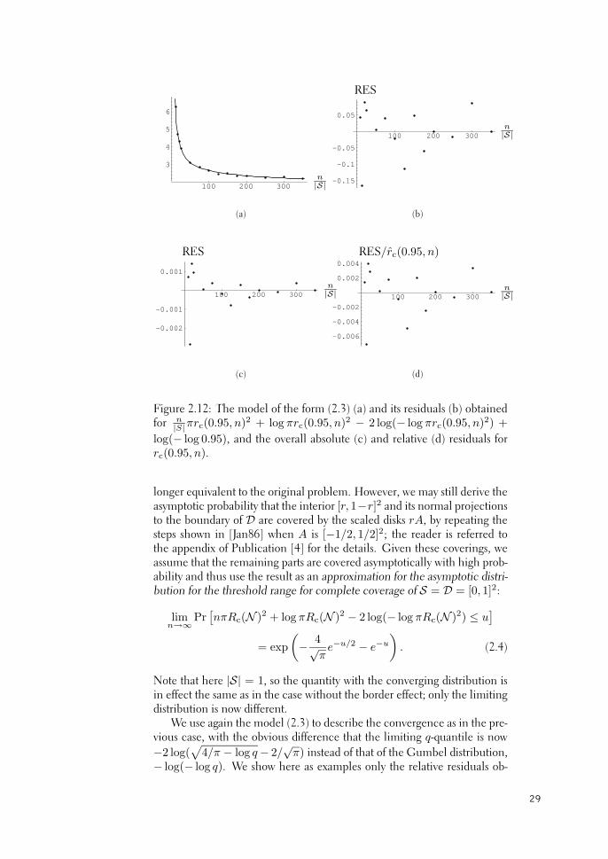
Probability of complete coverage as a learning problemWe now turn to the subproblem of determining the probability that Dis completely covered, i.e. Pr[C(N ,D, r) = 1]. In Publication [4], wepoint out that this problem, like the connectivity problem discussed ear-lier, also reduces to knowing the distribution of a well-defined thresholdrange: given D, let Rc(N ) denote the smallest sensing range r with whichD is completely covered by sensors at given locations N , i.e., with whichC(N ,D, r) = 1. We refer to Rc(N ) as the threshold range for completecoverage. Now, the event {C(N ,D, r) = 1} is equivalent to {r ≥ Rc(N )},whence this problem reduces to knowing the probability distribution ofRc(N ) with given n, S and D.
For given N , Rc(N ) is equal to the distance from a point in D to thenearest point in N , maximized over all points in D. It follows that Rc(N )can be easily determined using the sensors’ Voronoi diagram: it can be de-duced to be the longest distance from a sensor to an edge of its Voronoi cell
26
(a) (b)
Figure 2.11: Example of the threshold range for complete coverage whena) 25 sensors are placed randomly inside the square-shaped domain S = D,and b) sensors are scattered uniformly over the whole plane with averagedensity 25/|D|. The critical coverage ranges are shown with solid circles.
in D. Moreover, when the boundary of D is piecewise linear, it is suffi-cient to concentrate on cell corners. Like the expected area coverage, theprobability of complete coverage is strongly influenced by the border effect:Figure 2.11 shows examples of the threshold range determined for a square-shaped D, both when S = D and when the border effect is eliminated.
Recall that Theorem 2.2 gives the asymptotic distribution of the num-ber of sensors required on the set S to cover D completely, as their sens-ing range tends to zero. It also allows us to solve the inverse cumulativedistribution function of this number: to have D completely covered withprobability at least q, the number of sensors with range r must be at leastn(r) = [− log(− log q)− log πr2 + 2 log(− log πr2)] · |S|/πr2.
On the other hand, we may also want to know the inverse cumulativedistribution function of the threshold range for complete coverage, i.e., askhow large the sensing range should be with a given number of sensors n toguarantee a coverage probability of at least q: of course, the range shouldthen not be less than the smallest r with which the given n is at least n(r).By the continuity and monotonicity of n(r), it follows that r should be atleast r−1(n), the inverse function of n(r). We may thus conclude that The-orem 2.2 also holds with the given number of sensors n and the thresholdrange for complete coverage Rc(N ) substituted in the place of Nr and r,respectively. Because the resulting expression with the asymptotic Gumbeldistribution is a monotonically increasing function of Rc(N ) with given n,it follows that this result gives the asymptotic distribution of the thresholdrange for complete coverage when the number of sensors n tends to infinity.
The above observations provide the ingredients for treating the proba-bility of complete coverage as a learning problem, exactly as done and dis-cussed earlier with the connectivity probability. In what follows, we model
27
the convergence of the distribution of the threshold range for completecoverage using empirical models when D = [0, 1]2.
The purpose of requiring that the set S completely encompass D inTheorem 2.2 is to eliminate the border effect, i.e., to avoid complicationsresulting from the otherwise likely event that the boundary of D is the lastpart to be covered. In other words, Theorem 2.2 does not apply to the caseS = D demonstrated in Figure 2.11(a). We will next discuss the empiricalmodels in the setting without the border effect but will return to the caseS = D shortly.
To eliminate the border effect, the set S where the n sensors are ran-domly placed for each sample of the threshold range Rc(N ) is chosen as alarger square centered around the unit squareD. This other square is madelarge enough so that the resulting threshold range is never greater than theshortest distance from the boundary of D to that of S; this way, sensors out-side S would not affect the threshold range. (This requirement is checkedfor each sample of Rc(N ); if it is not met, the set S is enlarged furtherand all the simulations for the particular sensor density are repeated.) Aswhen simulating the threshold range for connectivity, Rc(N ) was deter-mined from 5000 random realizations of N with every fixed sensor densityn/|S|, and the value of n/|S| was varied up to 350.
Now, let rc(q, n) denote the q-quantile of Rc(N ). In the same spirit aswith the models in Publication [2], we let the model describe the deviationof n
|S|πrc(q, n)2 + log πrc(q, n)2 − 2 log(− log πrc(q, n)2) from its asymp-totic limit − log(− log q). Figure 2.12 is the equivalent of Figure 2.4, nowshowing as an example the corresponding information for these deviationsfor q = 0.95 along with a fitted four-parameter regression model of theform
i.e., a combined power-law where a slower-decaying component character-izes the tail of the model. In short, this figure allows for the same conclu-sions as Figure 2.4.
We now turn to the case S = D. In [Jan86], Janson is able to derivethe equivalent of Theorem 2.2 when S = D = [0, 1]2 and the set A isthe square [−1/2, 1/2]2 instead of the unit disk. In this case, covering Dcan be decomposed into the asymptotically seemingly independent eventsof covering the interior [r/2, 1 − r/2]2, i.e., the region where the effectof the randomly placed scaled squares rA is not affected by the boundaryof D, and covering its normal projections to the boundary such as {0} ×[r/2, 1 − r/2] with intersections of the overlapping squares, with length r.This is because when A is chosen as the square, covering the boundary ofD implies covering the strip between the boundary and the interior. Thus,the problem with border effects can be decomposed into subproblems inone and two dimensions, both free of border effects.
When A is chosen as the disk with unit radius as in Theorem 2.2 adaptedto our problem, covering the boundary ofD no longer implies covering thestrip between the boundary and the interior, and this decomposition is no
28
100 200 300
3
4
5
6
n|S|
(a)
100 200 300
-0.15
-0.1
-0.05
0.05
n|S|
RES
(b)
100 200 300
-0.002
-0.001
0.001
n|S|
RES
(c)
100 200 300
-0.006
-0.004
-0.002
0.002
0.004
n|S|
RES/rc(0.95, n)
(d)
Figure 2.12: The model of the form (2.3) (a) and its residuals (b) obtainedfor n
|S|πrc(0.95, n)2 + log πrc(0.95, n)2 − 2 log(− log πrc(0.95, n)2) +log(− log 0.95), and the overall absolute (c) and relative (d) residuals forrc(0.95, n).
longer equivalent to the original problem. However, we may still derive theasymptotic probability that the interior [r, 1−r]2 and its normal projectionsto the boundary of D are covered by the scaled disks rA, by repeating thesteps shown in [Jan86] when A is [−1/2, 1/2]2; the reader is referred tothe appendix of Publication [4] for the details. Given these coverings, weassume that the remaining parts are covered asymptotically with high prob-ability and thus use the result as an approximation for the asymptotic distri-bution for the threshold range for complete coverage of S = D = [0, 1]2:
Note that here |S| = 1, so the quantity with the converging distribution isin effect the same as in the case without the border effect; only the limitingdistribution is now different.
We use again the model (2.3) to describe the convergence as in the pre-vious case, with the obvious difference that the limiting q-quantile is now−2 log(
√4/π − log q− 2/
√π) instead of that of the Gumbel distribution,
− log(− log q). We show here as examples only the relative residuals ob-
29
100 200 300
-0.002
-0.001
0.001
0.002
0.003
n
RES/rc(0.5, n)
(a) q = 0.5
100 200 300
-0.015
-0.01
-0.005
0.005
0.01
n
RES/rc(0.99, n)
(b) q = 0.99
Figure 2.13: Relative residuals for two quantiles of Rc(N ), obtained byapplying the model (2.3) to the approximate asymptotic distribution (2.4)when S = D = [0, 1]2.
tained after fitting this model to 50% and 99% quantiles estimated fromsimulation data, again with 5000 samples generated for each n and n rang-ing up to 350: see Figure 2.13.
We opt to validate these models in Publication [4] only in the lattercase with S = D = [0, 1]2, i.e. when the models are based on the approxi-mate asymptotic distribution (2.4), since it is fair to assume that the modelsbased on the exact distribution in the case without border effects shouldperform at least as well. To this end, we test how well these models areable to predict the distribution of additional samples of Rc(N ) determinedfrom simulated random realizations with n = 1000 sensors; because of theresulting extensive computation times, only 1000 samples were generated.The result is shown in Figure 2.14: slight differences are noticeable, whichmay be due to the approximation (2.4), invalidity of the model (2.3), inac-curacy in the model parameter estimates, or the small number of samples
0.07 0.08 0.09
0.5
0.6
0.7
0.8
0.9
1
r
Pr[Rc(N ) ≤ r]
Figure 2.14: The empirical cumulative distribution of Rc(N ) determinedfrom 1000 random realizations with n = 1000 sensors in S = D = [0, 1]2
(solid line), and the predictions (drawn as points) of empirical models fittedto five different quantiles (indicated with the dashed lines).
30
in the validation data. However, the fact that the prediction errors are inboth directions makes a systematic error seem less likely.
2.3 Connectivity improvement as an optimization problem
In Publication [5], we view the connectivity problem from a new perspec-tive: we are concerned with what can be done when a wireless ad hocnetwork needs to be formed but the network nodes are too far apart to forma network with a desired level of connectivity. More precisely, we study theoption of improving the connectivity of a static ad hoc network by placingadditional network nodes at optimized locations. Networks where addingextraneous nodes is feasible are some sensor networks and such ad hoc net-works that are used in a controlled situation where some central entity canorganize the deployment of the nodes.
To our knowledge, the connectivity problem in ad hoc networks hasnot been addressed so far from this practical viewpoint: probably the closestrelated work has been done in [DTH02], where the authors study how theexistence of base stations attached to fixed, wired network infrastructureimproves the connectivity of random networks.
Problem statementsReusing the notation introduced in Section 2.1, we assume that the exist-ing network is disconnected and consists of n nodes with given locationsNin a bounded and convex deployment region D ⊂ R
d, d > 1, and that wemay place additional nodes in D to be used as relays in the network. Todistinguish between the two, we will refer to the existing nodes as terminalnodes and the additional nodes as relay nodes. We assume that the terminalnodes and the relay nodes have equal transmission and reception capabil-ities and hence have a common transmission range r. In this setting, thebasic form of our problem is as follows:
GivenN and r, find a set of locationsNr with minimum cardinalitynr that makes the geometric graph G(N
⋃Nr, r) connected.
Obviously, Nr is the set of locations to place relay nodes.We also study the following problem variant which comes into question
when too few relay nodes are available to make the network connected. Inthis case, we need to define the utility of the network.
Given N and r, find Nr that maximizes the chosen utility met-ric U = U(G(N
⋃Nr, r)), subject to nr ≤ nmax
r ∈ Z+.
The choice of the utility metric depends on the target application. Through-out Publication [5], we use the greatest number of terminal nodes that areall in the same connected component of the graph G(N
⋃Nr, r). In light
of the above problem, this is equivalent to using the greatest number ofterminal node pairs, i.e. the number of possible connections that can beformed within a connected component. In addition to this latter problem,we use the utility metric also in defining greedy approaches to the first prob-lem.
31
The key assumptions behind these problem statements are that the lo-cations of the terminal nodes are known and that the location informationof these nodes can be collected even though the network is not connected.The motivation behind the latter assumption is that depending on the so-lutions on the physical layer, it can be possible to be able to sustain a lowrate of communication over much further distance than to provide qualityof service. In this case, the network is able to convey control informationeven if efficient communications are not possible. In other words, in thisproblem the transmission range r models the longest distance that allowsdirect communication at the rate required by the application to be utilizedover the network.
Review of related problems and existing resultsThe closest related problem with existing literature is that of the Euclideanshortest-connection network, where the task is to form a connected net-work between a given set of points with minimum total edge length. Thisproblem has two variants, depending on whether or not the addition of newpoints is allowed before forming the edges: when permitted, the problem isknown as the minimum Steiner tree (or Steiner minimal tree) problem, andwhen not, it is the minimum spanning tree problem. Whereas finding theminimum spanning tree is a straightforward task, the Steiner tree problemis NP-hard [GGJ77]. A fundamental relation between the two problemsis the greatest possible ratio between their optimal solutions, known as theSteiner ratio [DH90b]: for any set of points in the plane, the total edgelength of their Euclidean minimum spanning tree is at most 2/
√3 ≈ 1.15
times the total edge length of their Euclidean Steiner minimal tree.Our problem in its basic form can be seen as a special variation of the
shortest-connection network problem, where the geometric graph providesthe edges implicitly and we are therefore restricted solely to adding newpoints. Accordingly, the objective function is then the number of addedpoints.
Our problem could as well be stated with the generalized goal of mak-ing the network k-connected. The corresponding generalization of theshortest-connection network problem without the possibility to add pointsleads to the graph augmentation problem: in commonly used terms, thetask in the minimum augmentation problem is to add to a given graph theset of edges with minimum total weight so that the resulting graph is k-connected. Thus, the case k = 1 corresponds to the minimum spanningtree problem, but for any k > 1 the problem is known to be NP-hard:see, e.g., [Hsu93] and the references therein. In this context, a somewhatrelated problem has been studied in [BR04], where an ad hoc network ofmobile robot nodes is already assumed to be connected, and the task is tomove the robots to make the network biconnected so that the total distancetravelled by the robots is minimized.
Heuristic algorithmsOur problem differs from the original shortest-connection network prob-lems, e.g., in that it is solely the addition of new points that it is all about;hence, unlike in the original counterparts, the objective function is integer-
32
valued. However, as we point out in Publication [5], our problem reducesto the shortest-connection network problem in the limiting case as r → 0:the optimal solution is then to place the relay nodes along the edges of theEuclidean minimum Steiner tree for N . In the general case, our problemposes the additional complication that we are not connecting only singlepoints to each other, but connected components in the graph G(N , r),where the best point for connecting to other components must be chosen.
Therefore, given the complexity of our problem, in Publication [5] wepropose heuristic algorithms that are applicable to both of its forms statedearlier. In what follows, we present these algorithms and conclude with abrief analysis of their performance. Our complexity analysis is to a large partbased on results gathered in [Aur91]; see the publication for more details.
Minimum Spanning Tree algorithm
Our first algorithm utilizes the minimum spanning tree: if we only requirethat each relay node or contiguous chain of relay nodes connect exactlytwo connected components of the graph G(N , r), the optimal solution is toplace the relay nodes along the edges of the Euclidean minimum spanningtree (MST) calculated for the components, when the distance between twocomponents is defined as the shortest distance between two terminal nodesin these distinct components. See Figure 2.15 for an example.
In fact, it is not difficult to show that this MST consists of exactly thoseedges of the MST for N that are longer than r. To this end, consider,e.g., Kruskal’s algorithm [Kru56] for finding the MST applied to the set ofpoints N : form the MST by drawing edges between points in the order ofincreasing length, drawing each edge only if it does not create a cycle withthe edges drawn earlier. It is easy to see that when we halt this algorithmat edge length r, the terminal nodes in any given subtree formed so far areexactly those in a connected component of the graph G(N , r), and hencethe rest of the algorithm also finds the MST for these components.
Figure 2.15: Minimum Spanning Tree algorithm. The initially connectedcomponents in this example realization of 70 terminal nodes are connectedwith solid edges, and the edges to place relay nodes are dotted. The trans-mission range is 10% of the side of the domain, as illustrated by the circle.
33
If the number of relay nodes available limits the solution, the optimal se-lection of edges of the MST to place nodes generally requires going throughall possibilities. In this case, we propose the greedy method of selectingedges in the order of added utility (with respect to the initial graph G(N , r))per used relay node. With this approach, the running time of the algorithmis in any case determined by that of finding the MST, which is O(n log n)in the plane.
Note that with a non-negligible transmission range, the Steiner rationo longer gives a valid approximation ratio for utilizing the MST in ourproblem: as a simple example, consider a regular pentagon whose verticesare on a circle with radius equal to the transmission range, and assumeone terminal node at each of these vertices. These initially disconnectedterminal nodes can be connected with a single relay node placed at thecenter of the circle, whereas the MST suggests placing as many as fourrelay nodes.
Greedy Tessellation algorithm
The stricter requirement that a single relay node should, when possible,join more than two connected components of the network suggests pointsthat are equally distant from several components as potential points of place-ment: our second algorithm is based on the observation that the pointsequally distant from three components are a subset of the vertices, i.e. thecoinciding corners of the convex sets also called cells, of the Voronoi di-agram of the existing nodes. Note that in practice, points equally distantto more than three nodes do not exist, but placing a relay node at a ver-tex close to other vertices may well result in connecting more than threecomponents.
This is the motivation for our Greedy Tessellation algorithm. In everyiteration of the algorithm, we examine the Voronoi diagram ofN
⋃Nr and
Figure 2.16: An example of the Greedy Tessellation algorithm, when ap-plied to the same realization as in Figure 2.15. The edges of the Voronoitessellation are shown with dotted lines, the candidate points for relay nodeinsertion with ’+’-signs. The first location to add a relay node is markedwith an asterisk.
34
regard as candidate points for node insertion the coinciding corners of suchVoronoi cells that contain nodes all in different connected components;the candidate point that yields the maximal increase in the chosen utilitymetric is added to Nr. Finally, if the candidate points are all further than rfrom the existing components, the remaining network is connected usingthe Minimum Spanning Tree algorithm. The final result is an algorithmthat takes O(n2) time in R
2 and O(n3) in R3 to connect the network.
Figure 2.16 illustrates the algorithm.
Greedy Triangle algorithmWith a closer look, we see that points equally distant from different com-ponents are not always optimal for relay nodes: the point equally distantfrom three given terminal nodes may fall outside the triangular convex hullof their locations, in which case it cannot be the optimal place for a relaynode to connect the three nodes (optimal in the sense that the range re-quired from the relay node to connect the terminal nodes is minimized).For example, the point marked in Figure 2.16 as the place for the first re-lay node is such a point. Thus, if looking only at the Voronoi diagram,one may not find all the places where connecting three components with asingle relay node is possible.
However, for given locations of three disconnected terminal nodes, theoptimal place for a relay node can be exhaustively determined: the pointequally distant from the terminal nodes is optimal only if it is inside the tri-angle spanned by the terminal nodes; if the point is outside the triangle, themidpoint of the longest side of the triangle is the optimal place. Similarly,
(a) (b)
Figure 2.17: Applying the Greedy Triangle algorithm to the realization ofFigure 2.15. (a): The first point to place a relay node in the first phase,as indicated by the ’+’-sign. Note the difference from Figure 2.16 in theplacement. (b): The first pair of points to place relay nodes, as determinedin the second phase, after several relay nodes have been added in the firstphase. Note that in this case, four components are connected.
35
one can find jointly optimal places for two relay nodes to connect three ter-minal nodes. Our analysis of this case, which is already more complicated,is presented in Appendix 4.
The analyses of the above two cases are the basis for our last algorithm.The Greedy Triangle algorithm proceeds through two rounds of iterations.The first round consists of repeatedly finding candidate triplets of terminalnodes that are all in different components and pairwise at most 2r apart,and connecting the triplet that yields the maximal increase in the chosenutility metric with a single relay node. This is then repeated in the secondround by connecting triplets at most 4r apart with two relay nodes in eachiteration. Finally, as in the Greedy Tessellation algorithm, the MinimumSpanning Tree algorithm is invoked to connect the network partitions thatremain. The result of one iteration in both the two rounds is illustrated inFigure 2.17. The running time of this algorithm is of the same order as inthe previous algorithm in two and three dimensions.
Comparison of the algorithmsFinally, we present results from applying our three algorithms to simu-lated realizations of randomly and uniformly distributed terminal nodes ina square-shaped domain in the plane. The purpose is partly to comparethe performance of the algorithms relative to each other, and in part togain some idea on how close to optimal their solutions are. The latter is aproblematic task, as the optimal solution for a general realization is usuallyunknown. We used as a benchmark the method of placing the relay nodeson those edges of the Euclidean minimum Steiner tree for N that connectdifferent components of the graph G(N , r). This method should be closeto optimal with sparse networks, i.e. when the transmission range is smallcompared to the typical distance between neighboring terminal nodes.
Figure 2.18(a) shows the average number of relay nodes needed to con-nect random configurations with varying number of terminal nodes usingeach of the different algorithms. The transmission range was set to 10% ofthe side of the square domain, in order to demonstrate a “feasible” scenariowhere the number of relay nodes needed is still a fraction of the number ofterminal nodes, making the addition of relay nodes sensible. As expected,our three algorithms produce gradually better solutions. The two greedyalgorithms also outperform utilizing the Steiner tree with these parameters,as the minimum Steiner tree simply optimizes the wrong measure from ourproblem’s viewpoint.
The gain from utilizing the Steiner tree is captured in Figure 2.18(b)which shows corresponding results with the transmission range set to 5% ofthe side of the domain. In a very sparse initial network, the existence ofsuitable candidate triangles is unlikely, and the Greedy Triangle algorithmpractically reduces to the Minimum Spanning Tree algorithm, while theSteiner tree yields the best results. As the density of the initial networkincreases, the Greedy Triangle algorithm surpasses the Steiner tree methodin performance.
The quantity that best describes what we referred to as the density of thenetwork is the average number of other terminal nodes directly connectedto a random terminal node in the initial configuration. Ignoring the bordereffect, this quantity is given by n/A ·πr2 where A is the area of the domain.
36
0 50 100 150 200 2500
5
10
15
20
25Minimum spanning treeGreedy TessellationGreedy TriangleEuclidean minimum Steiner tree
n
nr
(a)
5 10 50 100 150 200
30
40
50
60
70
80
90
Minimum spanning treeGreedy TriangleEuclidean minimum Steiner tree
n
(b)
Figure 2.18: Average number of relay nodes needed to connect the net-work, as a function of the number of terminal nodes initially in the network,taken over 1000 random realizations. (a): The transmission range is 10% ofthe side of the square-shaped domain. (b): The transmission range is 5% ofthe side of the domain; the Greedy Tessellation algorithm has been omittedfor clarity.
In essence, this quantity determines which method yields the best results,and for example the two greedy algorithms bring significant advantage overthe MST algorithm at proper intermediate values of this quantity, whensuitable candidate triangles are likely to exist.
2.4 Summary and Conclusions
This chapter focused on studies where wireless multihop networks are mod-eled with Boolean models. When used to describe the network topol-ogy, these models implicitly account for some constant-level backgroundnoise but not for interference from concurrent transmissions in the net-work. Thus, such a model is adequate for studying ultimate limits for con-nectivity, or connectivity in cases where interference is not a limiting factorfor communications. The latter is the case in networks with low transmis-sion activity or transmission powers, or when nodes are sparsely located andhence separated by long distances.
We first addressed the problem of determining the k-connectivity prob-ability of random, finite networks. Scenarios where this problem arises in-clude network dimensioning: for example, how densely should networknodes with given communication capabilities be scattered in order to havea k-connected network with high probability? As this problem is equivalentto knowing the distribution of the threshold range for k-connectivity, ourfirst approach to this problem was to model empirically the convergence ofthese distributions, studied by simulation, to their previously analytically de-rived asymptotic limits, allowing the prediction of the k-connectivity prob-ability for finite configurations. To this end, we developed algorithms to
37
determine the threshold range for 1-, 2-, and 3-connectivity for a given setof network nodes.
We also studied the connectivity of mobile networks, where n nodesare assumed to move according to the Random Waypoint (RWP) mobil-ity model. In this context, we applied an alternative approach, namely,an analytical approximation where the threshold range for k-connectivityis treated as the maximum of n i.i.d. k-nearest-neighbor distances, whichreflects the properties of the known asymptotic statistics.
Overall, because our empirical method is devoid of the systematic er-ror present when assuming that the asymptotic properties of connectivitystatistics also hold in the non-asymptotic regime, it provides the most ac-curate prediction results thus far. However, the requirements for using thisapproach with good results are that obtaining ample observations from fi-nite configurations is not an obstacle and that the asymptotic distribution isknown in analytical form; the case of RWP mobility is an example of wherethe latter does not hold true.
Next, we discussed the coverage of random networks under the Booleanmodel, which is of importance when dimensioning a sensor network withrandomly scattered nodes. In this context, we formulated the problem asthat of determining the distribution of the area coverage caused by ran-domly placed sensors in a bounded target domain. We showed that theexpected value of this distribution is equal to the probability that a randompoint in the domain is covered, making possible the analytical calculationof this quantity in a simple setting. We also addressed the problem of deter-mining the probability of full coverage and pointed out that this problem,like that of connectivity, is also equivalent to knowing the distribution ofa well-defined threshold range. We showed how to determine this rangefor a given set of nodes and target domain, and interpreted existing analyt-ical results as an asymptotic distribution of this threshold range. We alsoderived an approximate limit distribution of the threshold range in a casewith border effects. With all the same ingredients as with the connectivityproblem at hand, we also treated the problem of full coverage as a learn-ing problem, with the result of predicting the distribution of the thresholdrange for full coverage from independent simulations with good accuracy.To our knowledge, no analytical approximations aiming at accurately pre-dicting the probability of full coverage have been presented to date, whichmakes our empirical approach all the more important.
Finally, we presented a novel problem representing the algorithmic sideof connectivity research. The problem is motivated by a practical disaster re-covery scenario: given a disconnected network of terminal nodes deployedat known locations and the possibility of adding relay nodes with the sameproperties to the network, the task is to connect the network by adding aminimal number of relay nodes. We interpreted this problem as a specialvariation of the shortest-connection network problem and, in particular,pointed out its connection to the Euclidean minimum Steiner tree prob-lem, known to be NP-hard. We presented three increasingly advanced,centralized heuristic algorithms along with their complexity analysis, andcompared their performance by simulation. The more evolved algorithmsare most useful at proper intermediate densities of the initial network.
38
In the assumptions of the last problem, we precluded the mobility ofterminal nodes. The approach of adding relay nodes in optimized locationshas little application if all the terminal nodes tend to move all over the net-work region. However, by keeping track of the locations of terminal nodesover time, it should be possible to recognize those nodes that are nearlystationary and place relay nodes to connect these nodes. This question hasbeen taken under further study.
39
40
3 STUDIES UNDER THE PHYSICAL MODEL
The studies in this chapter have the assumption of the Physical model as thecommon denominator. The first section deals with generalizing the notionof connectivity to this model, and the second section discusses throughputin a particular network scenario.
3.1 Connectivity
In this section, we discuss connectivity when studied under the Physicalmodel. In this case, connectivity is subject to a more difficult choice ofdefinition than under the Boolean model. Whereas in the latter all thevariables that dictate whether two nodes can communicate directly can bewoven into a single parameter, viz. the transmission range within whichdirect connections exist, in the Physical model successful communicationalso depends on the interference from all other nodes that is time-varyingin nature. Thus, not only will the existence of a direct link between twonodes be governed by the locations of all nodes in the network, but thecondition for its existence should be defined with this temporal aspect inmind. On the other hand, the dependence on the interference means thatconnectivity is also affected by medium access control.
The existing literature on connectivity under the Physical model issparse in comparison to that under the Boolean model; we will begin witha review of earlier studies.
Review of existing resultsThe pioneering work in assessing the impact of interferences on connec-tivity has been made in [DBT03] (see also the journal version [DBT05])where the authors study a CDMA network. In line with the Physical model,they assume that node j can successfully receive the signal transmitted bynode i if and only if
Pi · l(||xi − xj ||)N0 + γ
∑k 6=i,j Pk · l(||xk − xj ||)
≥ T, (3.1)
where the factor 0 ≤ γ ≤ 1 weighting the interference power sum is moti-vated by the partial orthogonality of CDMA codes and can be interpretedas the inverse of the processing gain of the system. Neglecting unidirec-tional links, an undirected edge is assumed to exist between nodes i andj if and only if (3.1) also applies with i and j interchanged; the resultinggraph is named the Signal To Interference Ratio Graph (STIRG). Note thatthe case γ = 0 reduces to the Boolean model.
Recently refined from the initial result presented in [DBT03, DBT05],it is then shown in [DFM+06] that in an infinite STIRG whose nodes arelocated on the points of a Poisson process on R
2 and transmit with somecommon power, i.e. Pi ≡ P , percolation occurs when the node density λis greater than the much-studied critical intensity λc of the case γ = 0 (with
41
the given T · N0/P ), provided that γ is sufficiently small (but not zero).More precisely, assuming that the attenuation function l(·) ≤ 1 is con-tinuous, strictly decreasing, and satisfies some additional non-degeneracyconditions, for any node density λ > λc(T ·N0/P ), there exists γ∗(λ) > 0such that for γ ≤ γ∗(λ), the graph has an infinite connected component.In [DT04], it is further shown that as λ tends to infinity, the condition forthe occurrence of percolation is that either γ∗(λ) or the SINR thresholdT must decrease at least as fast as 1/λ. Since decreasing γ requires using awider frequency band and decreasing T implies a lower rate of communica-tion, this means in either case that the available transport capacity per fixedbandwidth decreases. This establishes thus a trade-off between connectivityand capacity.
Also an infinite random network, but employing slotted Aloha insteadof CDMA, is analyzed in [BBM04, BBM06]. In the presented mediumaccess scheme, time is slotted and each node is allowed to transmit in anyslot with a fixed medium access probability p. The condition for node jsuccessfully receiving node i’s transmission in any time slot – producingwhat is chosen as the unit throughput from i to j over this time slot – nowbecomes
Pi · l(||xi − xj ||)N0 +
∑k 6=i,j ekPk · l(||xk − xj ||)
≥ T, (3.2)
where ek is the indicator variable of the event that node k is allowed totransmit in that time slot. The individual permissions to transmit are in-dependent among both nodes and time slots, so that the variables {ek}in every time slot are independent Bernoulli-distributed random variableswith parameter p.
In this study, connectivity is defined as a dynamic property: the au-thors show that slotted Aloha allows the transmission of packets over timefrom any node to any other node, under simple independence and non-degeneracy assumptions on node mobility, and also in the case withoutmobility if N0 = 0, i.e., if there is no background noise. However, this def-inition places no requirements on the long-term rate of successful commu-nication and can therefore be regarded as coincident with the omnipresentinformation-theoretic connectivity discussed in Chapter 1.
Thus far, in the context of network models that account for interference– such as the Physical model – little has been done to address connectivityof finite networks as defined in graph theory, namely, the requirement thatall node pairs be connected through the network. The aim in Publication[6] is to take a first step in this direction.
Studying graph connectivity under the Physical modelIn Publication [6], we generalize the notion of the threshold range for con-nectivity from the Boolean model to the Physical model. We do this underthe two scenarios reviewed above, i.e., assuming first a CDMA network andthen a network using slotted Aloha. As we will see, since there is more thanone free parameter in these scenarios, unlike in the Boolean model char-acterized solely by the transmission range, the threshold range generalizesinto a boundary in the space of these parameters. This boundary consistsof segments of individual link connectivity constraints that are linear with
42
respect to at least some of the free parameters, and it can be traced in theparameter space by keeping track of the prevailing network topology and, inparticular, the critical link for connectivity by applying a very simple rule.
Like in the definition of the threshold range under the Boolean model,we also assume throughout that all network nodes employ some commonconstant transmission power P . Further, although not at all necessary, werestrict ourselves to the commonly used power-law attenuation function
l(||xi − xj ||) = (C||xi − xj ||)−α, (3.3)
to allow easy scaling of any configuration of network nodes to arbitrary phys-ical node densities. Here, C > 0 sets the scale and α > 2.
Connectivity boundary in a CDMA networkWe begin with the conceptually simpler scenario with the CDMA net-work which allows easy and unambiguous determination of the connectiv-ity boundary. We will derive this boundary for a STIRG graph representinga network with given node locations {xk} and a fixed attenuation exponentα in the above attenuation function. As in [DBT03], we assume that allnodes transmit constantly, representing a worst-case scenario. In this case,(3.1) is equivalent to
A ≤ −B∑
k 6=i,j
||xk − xj ||−α + ||xi − xj ||−α, (3.4)
where we have defined the two free parameters A = Cα TP/N0
and B = Tγ.Hence, in a given network, the condition for node j successfully receivingnode i’s transmission is satisfied on and below the descending line in theB/A-plane with slope −
∑k 6=i,j ||xk −xj ||−α and intercept ||xi−xj ||−α,
both of which we may calculate (see Figure 3.1 for three instances of suchlines). Since our attenuation function is reciprocal, i.e. l(||xi − xj ||) =l(||xj −xi||), which can also be said to hold in reality on a fixed frequency,the resulting condition for an edge existing between nodes i and j in theundirected STIRG is determined by this common intercept and the steeperone of the two slopes calculated in both directions (i.e., the receiver undermore noise).
The domain in the B/A-plane in which the given network is connectedthen lies below a connected curve consisting of segments of descendinglines, representing the constraints of different links that are critical for net-work connectivity at each point; this curve is the connectivity boundary(see Figure 3.1 for an example). It can be found as follows. Start at B = 0,whence γ = 0. This makes the model coincide with the Boolean model,meaning that that the critical link is found as the longest edge in the Eu-clidean minimum spanning tree of the nodes. The descending line corre-sponding to this link determines the boundary of the connectivity region aslong as no line of the other links is crossed. When this happens, we maydetermine the new critical link using the following simple rule:
• When a line is crossed from below (as in the first intersection encoun-tered in Figure 3.1 when increasing B from 0), i.e. the connectivity
43
0.02 0.04 0.06
2
4
6
8
10
12
14
16
B = Tγ
A = Cα TP/N0
Figure 3.1: The connectivity domain of the network of Figure 3.2 whenα = 3. The solid line indicates the border of the domain. Taking A = 0implies neglecting background noise; the case γ = 0 ⇒ B = 0 impliesneglecting interference.
region of another link is left when tracing the current line, the corre-sponding disappearing link is the critical link from this point onwardsif the remaining links no longer form a single connected graph. Oth-erwise, the critical link does not change.
• When a line is crossed from above (as in the second intersection ofFigure 3.1), i.e. the connectivity region of another link is enteredwhen tracing the current line, the corresponding appearing link isthe critical link from this point onwards if it connects the two net-work partitions separated by the current critical link. Otherwise, thecritical link does not change.
As an example, Figure 3.1 shows the resulting connectivity boundary of thenetwork in a unit square shown in Figure 3.2.
In this model, we assumed that all other nodes transmit constantly. Itwould of course be more reasonable to assume that at least half of the nodesare receiving instead of transmitting at any instant. In general, if we assumethat on average every kth node is transmitting, we should regard γ as ageneral interference thinning factor γ = γ/k, where γ is the actual codeorthogonality factor.
Connectivity in a slotted-Aloha networkWe then extend the definition of the connectivity boundary to the slotted-Aloha network. In addition to the node locations and the attenuation expo-nent, we assume that the medium access probability p has been fixed. Theequivalent of (3.4) is now
A ≤ −T∑
k 6=i,j
ek||xk − xj ||−α + ||xi − xj ||−α, (3.5)
where the sum∑
k 6=i,j ek||xk − xj ||−α is a random variable independentin every time slot, having a discrete probability distribution with generally
44
1
2
3
4
5
67
8
9
10
(a)
1
2
3
4
5
67
8
9
10
(b)
1
2
3
4
5
67
8
9
10
(c)
1
2
3
4
5
67
8
9
10
(d)
Figure 3.2: An example network in the unit square. The prevailing topologywith the identified critical links have been drawn at each of the vertices ofthe border in Figure 3.1. The dashing of the links corresponds to that usedin Figures 3.1 and 3.3.
2n−2 distinct possible values, with n denoting the number of all the networknodes. Given the assumed information, we may calculate this distribution.
In addition to the free parameters A = Cα TP/N0
and T , we then definea third parameter, link confidence q. For a given q, the q-quantile of thedistribution of the above random sum describing the scaled interferencegives the level below which the latter remains with confidence (probability)q for each directed link i → j. The difference from the previous sectionis that instead of the function fij(γ) = γ
∑k 6=i,j ||xk − xj ||−α that can
be seen in (3.4), which is linear in its argument 0 ≤ γ ≤ 1, we now havethe nonlinear function F−1
ij (q) where Fij(·) is the cumulative distributionfunction of the random sum
∑k 6=i,j ek||xk − xj ||−α. (To be exact, we
45
define the inverse function of this discrete-valued cumulative distributionas F−1
ij (q) = min{t : Fij(t) ≥ q}.) Because of this nonlinearity, theparameter q can no longer be incorporated into the second free parameterwith T but has to be treated as a separate, third parameter. Note howeverthat the two functions fij(γ) and F−1
ij (q) coincide at γ = q = 1.The connectivity boundary is a surface in the space of the three free
parameters A = Cα TP/N0
, T , and q, a cross-section of which with fixed q
looks similar to Figure 3.1: (3.5) can be written in the form
A ≤ −F−1ij (q) · T + ||xi − xj ||−α, (3.6)
which, with fixed q, is satisfied on and below the descending line in theT/A-plane with slope −F−1
ij (q) and intercept ||xi − xj ||−α. As in theprevious section, we define the condition for nodes i and j being bidirec-tionally connected to be determined by the steeper slope, i.e., the greaterinterference with the given confidence q.
With any fixed q, the cross-section of the connectivity boundary in theT/A-plane is found exactly as in the previous section, by tracing along thecritical links. The reason why the longest edge in the Euclidean mini-mum spanning tree is again the critical link as T → 0 is that in thislimit, the above condition (3.6) for every link is dominated by the intercept||xi − xj ||−α which is a monotonically decreasing function of the link dis-tance.
To demonstrate the connectivity boundary in this case, we examineagain the example network of Figure 3.2. We assume that α = 3 andtake p = 0.1, the latter representing a magnitude found suitable for themedium access probability in [BBM04]. Figure 3.3 shows the connectivitydomain in the T/A-plane with q fixed to different values; it is easy to seethat q = 1 leads to the domain of Figure 3.1 with T in the place of B. Theconnectivity surface of the network in the space of all three parameters isdepicted in Figure 3.4.
Next, we will show that the connectivity requirement in the slotted-Aloha network constitutes a boundary condition for a tradeoff between thedelay and throughput of the network links and allows for an optimizationbetween the two as desired.
To this end, recall that the link confidence q defines when a pair ofnodes is considered directly connected: we say that there is a link from anynode i to any other node j only if, with given parameters A = Cα T
P/N0
and T , the probability q that (3.2) holds in a random time slot is at least q.Assume that the conditions for a completely successful transmission from ito j are that (i): node i is allowed to transmit, (ii): node j does not transmitin the same time slot, and (iii): the states of the remaining nodes are suchthat (3.2) holds. Then, due to the nodes’ independent operation, the num-ber of time slots needed for one successful transmission from i to j obeysa geometric distribution with parameter p(1 − p)q. Furthermore, for thecritical link in a network with many nodes it is reasonable to assume thatq ≈ q. Hence, requiring a higher link confidence means requiring a lowermaximum average link delay in the network, whereas allowing a lower linkconfidence means allowing a higher maximum average link delay.
46
0.05 0.1 0.15 0.2 0.25 0.3
2
4
6
8
10
12
14
16
T
A = Cα TP/N0
(a) q = 0.85
0.25 0.5 0.75 1 1.25 1.5
2
4
6
8
10
12
14
16
T
A = Cα TP/N0
(b) q = 0.65
1 2 3 4
2
4
6
8
10
12
14
16
T
A = Cα TP/N0
(c) q = 0.45
1 2 3 4
2
4
6
8
10
12
14
16
T
A = Cα TP/N0
(d) q = 0.40
Figure 3.3: The connectivity domain of the network of Figure 3.2 whenα = 3 and p = 0.1, with the boundary indicated by a solid line whereneeded. Note that in this case, there is no interference in an arbitrary timeslot with probability (1−0.1)8 ≈ 0.43, hence the zero-slope with q = 0.40.
01
23
4
0.4
0.6
0.8
1
0
5
10
15
12
34
A
TT
q
Figure 3.4: The surface below which the network of Figure 3.2 is connectedwhen α = 3 and p = 0.1. The cross-section of the surface is as in Figure3.3(d) for all q ≤ (1− 0.1)8 ≈ 0.43.
47
On the other hand, the probability p(1 − p)q is also the proportion oftime slots with successful transmissions from node i to j over time. Thedefined unit throughput of each successful transmission in turn dependson the SINR threshold T : if we take as a reference the Shannon capacityof a channel with Gaussian noise and interference and a given SINR, thisis proportional to log(1 + SINR). Then the minimum time-averaged linkthroughput in the network is proportional to q log(1 + T ).
The two parameters q and T that together determine the maximum av-erage link delay and the minimum link throughput are bound together bythe connectivity constraint, which dictates that the greatest achievable Tdepends on the required q: Tmax = Tmax(q). For a given network, the re-quired link confidence q can be increased from zero to some positive valuewithout sacrificing minimum link throughput (with our example network,we know that this value is at least q = (1 − 0.1)8). The maximum of theminimum link throughput with respect to q marks the beginning of Pareto-optimal combinations of maximum link average delay and minimum linkthroughput, meaning that neither quantity can be improved without mak-ing the other quantity worse: beyond this maximizing value of q, a delay-throughput tradeoff must then be made according to design preferences.
The computational task of determining the distribution of the interfer-ence from a given network of n nodes for a given transmitter-receiver pairgrows exponentially with n, as it entails evaluating all the possible 2n−2 val-ues of the interference and their probabilities. The end of Publication [6] isdevoted to presenting a computationally efficient method for determiningan approximation for this distribution.
3.2 Throughput
This section addresses throughput in networks under the assumptions of thePhysical model, both as an aggregate quantity in the whole network and asexperienced by an individual node. The most fundamental existing results,which we will discuss first, concern the highest achievable throughput un-der the restrictions of this model.
Review of existing resultsThe aim in the study [GK00] that first presented the Physical model is todetermine bounds and scaling laws for the achievable throughput underthat model. For this purpose, the authors define bit-meter as the basic unitof information transfer in the network, and the transport capacity of thenetwork as the bitrate-distance products summed over all concurrent single-hop transmissions taking place in the network, measured in bit-meters persecond, in analogy with, e.g., the passenger-kilometers-per-year metric usedby airlines.
The authors then derive bounds for the best-case transport capacityachievable in arbitrary networks, where the various parameters such as nodelocations, transmission powers and the traffic pattern can be arbitrarily op-timized. The main result, further refined in [AK04], is that for a net-work of n nodes in a domain with area A under the Physical model andthe power-law attenuation function (3.3), when the maximum transmission
48
power is bounded by Θ(nα), the transport capacity has the upper boundΘ(√
An). This bound is sharp, in the sense that it is also an achievablelower bound. Furthermore, in the case without power constraints, the up-per bound O
(n
α−1α
)holds.
In [BBM04, BBM06], Baccelli et al. analyze infinite random slotted-Aloha networks where the transmission powers are assumed independentrandom variables with identical probability distribution. The authors definean alternative throughput measure, the spatial density of progress, whichis measured in bits per second crossing a meter of the line perpendicularto the direction of transfer in the planar network. The mean density ofprogress is proposed as the optimization criterion in selecting the mediumaccess probability p; the optimal value depends only on the required SINRthreshold T and, more importantly, not on the density of nodes. This makesa decentralized implementation possible, provided that nodes have somelocal information on the location of other nodes. In contrast, the authorspoint out that for optimal spatial reuse and hence optimal throughput scal-ing in a network using CSMA, the range within which one transmissionshould be prohibited from another depends on the density of nodes, whichis an impediment to the decentralized implementation of CSMA in wire-less multihop networks.
Translating the mean density of progress to Gupta and Kumar’s trans-port capacity, it is then shown in [BBM04] that a network with node den-sity λ in the infinite plane transports Θ(
√λ) bit-meters per second, per
unit area, which is equivalent to the above bound Θ(√
An). Thus, the up-per bound for the scaling of transport capacity in multihop networks is infact reached by random networks using slotted Aloha. This, along with thepossibility for decentralized implementation, certainly makes this simplerandom-access scheme seem appealing.
Most of the quantitative analysis in [BBM04] assumes that the randomtransmission powers of the nodes are exponentially distributed and henceunbounded. In Publication [7], we extend the analysis by departing fromthis assumption, and evaluate the probability of successful transmission –or, more aptly, reception – when all nodes transmit with a common con-stant transmission power. As the basis of the more evolved analysis alsoin [BBM04], this probability is one of the most fundamental performancequantities in the network and, as pointed out using the concept of link con-fidence in the previous section, also determines the long-term throughputof any given link. We discuss this in more detail in what follows.
Probability of successful transmission in a random slotted-Aloha networkWe begin by briefly going through the network modeling assumptions. Asin [BBM04], the network that we study is infinite, with nodes located atthe points of a Poisson point process Φ = {Xi} with intensity λ on theplane R
2. As with most results in [BBM04], we also assume the power-law attenuation function (3.3) and that the power of the background noiseN0 = 0, so that the condition for successful reception reduces to the one forthe Signal-to-Interference Ratio (SIR). We remark, however, that since theevaluation of the probability of successful transmission reduces to that of the
49
distribution of the random interference, the assumption N0 = 0 is mademerely to allow compact results; in a practical scenario with numericalparameter values available, the following work could easily accommodatea non-zero noise power.
This setting where we neglect the background noise is equivalent to theextreme limit of an interference-dominated case, which results when trans-mission activity is high and the transmission powers or the spatial densityof the network nodes is increased: these changes all have the same effectof diminishing the parameter A introduced in the previous section. Thiscan be contrasted with the noise-dominated case which results under theopposite conditions and whose extreme limit is equivalent to the Booleanmodel.
Problem statementUnder the above assumptions, by the properties of the homogeneous Pois-son process the probability of node i at xi successfully receiving node j’stransmission only depends on the distance d = ||xj − xi|| and not on thespecific locations xi, xj . Thus, without loss of generality we may select xi
as the origin, whence the condition for successful reception can be writtenin the following equivalent forms:
P (Cd)−α
I≥ T ⇔ I ≤ P (CT 1/αd)−α
⇔ I
P (CT 1/αd)−α=
∑k
ek
(||Xk||T 1/αd
)−α
≤ 1, (∗)
where I =∑
k ekP (C||Xk||)−α is the interference power sum at the re-cipient. In Publication [7], we are interested in the probability that thiscondition holds given d. However, as will next be explained, we take adeeper look at this quantity than was done in [BBM04].
First of all, we may ask what is the probability, accounting for boththe random locations {Xk} and medium access states {ek} of all othernodes, that (∗) holds in a random time slot. In other words, if a randomconfiguration {Xk} is observed in a random time slot, what is the proba-bility that (∗) holds, given the distance d? Let us write this probability asPr{Xk},{ek}[(∗) holds | d]. This is the probability that was derived analyt-ically for exponentially distributed transmission powers in [BBM04], andwhich we will discuss first.
Then we study the probability that (∗) holds in a random time slot fora given configuration of surrounding nodes {Xk} = {xk} representing– and completely characterizing – the interference environment of onereceiving node in the network; we write this conditional probability asPr{ek}[(∗) holds | d; {Xk} = {xk}]. This probability is different for dif-ferent configurations {xk}, but it is fully determined once given the {xk}.It is thus a function of the random node locations {Xk} and therefore itselfa random variable with a probability distribution over {Xk}. This distri-bution describes how different nodes in the network are in different posi-tions with regard to the success of communication. In fact, the probabilityPr{Xk},{ek}[(∗) holds | d] discussed in the next section can be seen to bethe expected value of this distribution over {Xk}.
50
Probability of successful reception: expected value over {Xk}We begin with the probability that (∗) holds for a random configuration{Xk} in a random time slot, given the distance d of the transmitting nodefrom the receiver. Determining this probability reduces to knowing the dis-tribution of the random interference power sum I ; as will become evidentshortly, the Laplace transform of such a power sum is known in closed form,up to a certain integral. In our case, this integral requires resorting to nu-merical evaluation, making the inversion of the Laplace transform difficult.For this reason, we utilize a decomposition of the total interference powerinto two parts. By deriving the distribution of the interference power fromsome neighborhood of the receiver exactly, we are left with the remain-ing interference whose distribution can be deduced to be approximatelyGaussian; the larger that neighborhood, the smaller the difference. TheGaussian approximation can be improved by utilizing the known Laplacetransform with the aid of so-called Bahadur-Rao approximation. This way,combining the exact distribution of the near-by interference power and theapproximate one of the remaining interference, we obtain a numerical ap-proximation for the probability we are interested in that can be improvedto an arbitrary level of accuracy. We sketch out the details in what follows.
Because we are interested in any random configuration for only onetime slot, we may limit our attention in any configuration to the nodesthat transmit in that time slot. By the properties of the Poisson process,we may then write the interference power sum in (∗) as I = IΦ(λp) =P
∑k(C||Yk||)−α, the shot noise of a Poisson process {Yk} with intensity
λp at the origin. As pointed out in [BBM04], the Laplace transform of ageneral Poisson shot noise IΦ(λ) with i.i.d. transmission powers Pk ∼ P ,calculated at the origin, is
I∗Φ(λ)(s) = exp(−λ
∫R2
1− EP[exp(−sP(C||x||)−α)
]dx
). (3.7)
The generalization of the above to the interference at the origin from trans-mitters in some arbitrary domain simply amounts to integrating over thatdomain instead of R
2.Let Pr denote the power received from a transmitter at distance r, i.e.
Pr = P (Cr)−α = PT 1/αd
(r
T 1/αd
)−α. By (3.7), the Laplace transform ofI is now
I∗Φ(λp)(s) = exp[λp2π
∫ ∞
0
(e−sP
T1/αd
“r
T1/αd
”−α
− 1)
r dr
],
from which it follows that
I∗Φ(λp)
(s
PT 1/αd
)= exp
[λp2π(T 1/αd)2
∫ ∞
0
(e−st−α − 1
)t dt
],
(3.8)where the last expression can also be seen as the Laplace transform ofI/PT 1/αd. Note that it is precisely I/PT 1/αd whose distribution we areinterested in, since (∗) is also equivalent to I/PT 1/αd ≤ 1. (With a pos-itive background noise power N0, the corresponding condition would beI/PT 1/αd ≤ 1 − N0/PT 1/αd, the probability of which reduces to zero as
51
the distance d reaches the value with which PT 1/αd = N0; this value equalsthe transmission range of the Boolean model.)
A closer look reveals that I/PT 1/αd has infinite expectation and vari-ance. This is a side effect caused by the assumed power-law attenuationfunction (3.3) which has a singularity at zero distance. This shortcoming isimplicitly dealt with by the following decomposition of the interference.
We will treat the total interference power I as the sum of two parts.The distribution of one part is approximated using its Laplace transform,whereas the distribution of the other part is calculated exactly. The keyobservation allowing this division is that for (∗) to hold, there may be atmost m active transmitters at distances y satisfying
P (Cd)−α
(m + 1)P (Cy)−α< T ⇔ y < [(m + 1)T ]1/αd
def= rm,
i.e., m+1 active transmitters alone at distance rm would still satisfy the con-dition (∗), but moving them any closer would violate this condition. Now,we will partition the total interference power into two parts originating fromdifferent zones, i.e. IΦ(λp) = I = Iin + Iout, where Iin denotes the interfer-ence power originating from distances up to rm and Iout denotes that fromdistances beyond rm (see Figure 3.5).
Distribution of Iin
Because of the above limitation to at most m active transmitters withinrm, we may determine the distribution of Iin exactly, as follows. By theproperties of the Poisson process, given the number of nodes in the innerzone, their locations in that zone are i.i.d. uniformly distributed. Thus, thedistribution of the interference I1 from a single node in this zone can beeasily determined: denoting by R the distance of the node from the origin
d
rm = [(m + 1)T ]1/αd
Iin
Iout
Figure 3.5: Division of the interference into that originating from twozones, for some (m + 1)T > 1
52
and noting that I1 = PR = PT 1/αd
(R
T 1/αd
)−α def= PT 1/αdQ where PT 1/αd
is constant, we easily obtain the probability density of Q as
fQ(q) =
{2
α(m+1)2/α q−(2+α)/α, q > 1m+1 ,
0, q ≤ 1m+1 .
The total interference power from i nodes in the inner zone is then the sumof i.i.d. random variables PT 1/αd·
∑ij=1 Qj , where the probability density of∑i
j=1 Qj is obtained as the convolution of i instances of the above densityfQ(q), which we denote by f∗iQ (q). Given the condition that there are atmost m active transmitters within rm, the conditional distribution of Iin
is then obtained by conditioning on i with the Poisson distribution withparameter λpπr2
m, truncated at m:
fIin/PT1/αd
(q) =
∑mi=0
(λpπr2m)i
i! f∗iQ (q)∑mk=0
(λpπr2m)k
k!
.
For example, with m = 2 this conditional distribution can still be calcu-lated analytically (see Publication [7]).
Distribution of Iout
Let us next turn to approximating the distribution of Iout. Applying (3.7)again yields the Laplace transform
I∗out(s) = exp[λp2π
∫ ∞
rm
(e−sPrm( r
rm)−α
− 1)
r dr
]
⇒ I∗out
(s
Prm
)= I∗out
(s
PT 1/αd/(m + 1)
)
= exp[λp2πr2
m
∫ ∞
1
(e−st−α − 1
)t dt
],
where the last expression can also be seen as the Laplace transform of
Jdef= Iout/Prm
= (m + 1)Iout/PT 1/αd. After a change of variables u =t−(α−2), we then have for the logarithmic moment generating functionϕ(β) = log E
[eβJ
]= log J∗(−β) of J ,
ϕ(β) = 2λpπr2m
∫ ∞
1
(eβt−α − 1)t dt =2λpπr2
m
α− 2
∫ 1
0
eβuα/(α−2) − 1uα/(α−2)
du,
ϕ′(β) =2λpπr2
m
α− 2
∫ 1
0
eβuα/(α−2)du, (3.9)
ϕ′′(β) =2λpπr2
m
α− 2
∫ 1
0
uα/(α−2)eβuα/(α−2)du,
which yields, e.g., the mean and variance of Iout as E[Iout] = Prmϕ′(0)
and Var[Iout] = P 2rm
ϕ′′(0).Now, consider generating a random realization of Iout, taking only
nodes within some maximum distance into account for conceptual sim-plicity. This can be done by drawing the Poisson-distributed number of
53
interfering nodes, placing these nodes independently and uniformly at ran-dom on the considered domain, neither closer than rm nor further thanthe maximum distance, and calculating Iout as the sum of the individualinterference powers. Thus, Iout is the sum of i.i.d. random variables, andhence, by the Central limit theorem (see, e.g., [Lin22]), should obey a dis-tribution that tends to the Gaussian as the node density tends to infinity.More precisely, provided that the density is so large that there is likely tobe many nodes at the smaller distances with nearly equal contributions toIout, the distribution of Iout – and hence that of the scaled quantity J –should be close to Gaussian.
Note that given α, the distribution of J is fully characterized by theproduct λp r2
m. In fact, the quantity λpπr2m is the expected number of trans-
mitting nodes within distance rm from an arbitrary reference point. Thisquantity also determines how close to Gaussian the distribution of Iout –and hence J – is: if this number is small, then the total interference poweris likely to be dominated by few terms, resulting in a distribution far fromthe Gaussian. Accordingly, the larger the value, the better the Gaussianapproximation. Figure 3.6 shows how the Gaussian approximation agreeswith the simulated distribution of J with different values of λpπr2
m. To fa-cilitate the simulation, interference from distances beyond k · rm, with k
0.2 0.4 0.6 0.8 1 1.2
0.2
0.4
0.6
0.8
1
t
Pr(J ≤ t)
(a) λpπr2m = 0.1
0.5 1 1.5 2 2.5
0.2
0.4
0.6
0.8
1
t
Pr(J ≤ t)
(b) λpπr2m = 0.4
0.5 1 1.5 2 2.5 3 3.5 4
0.2
0.4
0.6
0.8
1
t
Pr(J ≤ t)
(c) λpπr2m = 0.8
1 2 3 4 5
0.2
0.4
0.6
0.8
1
t
Pr(J ≤ t)
(d) λpπr2m = 1.2
Figure 3.6: Cumulative distribution of J = Iout/Prmwith different values
of λpπr2m when α = 3. The simulation domain has been defined using
chosen to be some large number, was neglected; this changes the results in(3.9) so that the upper limit ∞ in any of the integrals now becomes k andthe lower limit 0 becomes k−(α−2). One can see in the figure that the accu-racy of the approximation indeed improves as λpπr2
m increases, but the fitat the tails of the distribution remains poor. This can be remedied by adopt-ing an approximation from large deviations theory (see [BR60, Section 6])and applying it also below the mean; this approximation is introduced inthe appendix of Publication [7]. This Bahadur-Rao (BR) approximation sig-nificantly improves the fit in the tails, while it coincides with the Gaussianapproximation at the mean of the distribution: it is also shown in Figure3.6.
Adding up Iin and Iout
We may now combine the means to evaluate the distributions of Iin andIout to obtain an approximation for the probability that (∗) holds: this canbe written as
Pr [(Iin + Iout)/PT 1/αd ≤ 1]= Pr(at most m active transmitters within rm)
×∫ 1
0
fIin/PT1/αd
(q)Pr [Iout/PT 1/αd ≤ 1− q] dq
= e−λpπr2m
m∑k=0
(λpπr2m)k
k!
∫ 1
0
∑mi=0
(λpπr2m)i
i! f∗iQ (q)∑mk=0
(λpπr2m)k
k!
× Pr[(m + 1)Iout/PT 1/αd ≤ (m + 1)(1− q)]dq
= e−λpπr2m
∫ 1
0
m∑i=0
(λpπr2m)i
i!f∗iQ (q)Pr[J ≤ (m + 1)(1− q)]dq. (3.10)
The accuracy of different approximations for Pr{Xk},{ek}[(∗) holds | d] isdemonstrated in Figure 3.7. In comparison, we point out that the Laplacetransform (3.8) of I/PT 1/αd can also be used directly, by applying the BRapproximation; this method has also been included in the figure and canbe seen to result in a very poor approximation. On the other hand, using(3.10) with m = 2 already proves to be notably accurate and gives a sig-nificant improvement from using m = 0. One may also note in Figure3.7(a) how the probability behaves differently under the assumption of ex-ponentially distributed transmission powers. In particular, the probabilitymakes a sharper transition with increasing distance d in our case. This isbecause the signal-to-interference ratio at reception varies less due to thelack of randomness in the transmission powers.
Note that we can improve the approximation to any level of accuracy bychoosing sufficiently large m. The gain from increasing m is twofold. First,through increasing λpπr2
m, it makes it possible to approximate the distri-bution of J more accurately, as shown by Figure 3.6. Second, it decreasesthe share of Iout in the total interference, thus mitigating the effect of theremaining inaccuracy. The cost of increasing m is the added numericallabor in computing further convolutions f∗iQ (q).
We conclude by noting that a similar decomposition of interferers intonear-by and distant ones is used in [WYAd05], in determining upper and
55
0.2 0.4 0.6 0.8
0.2
0.4
0.6
0.8
1
t
Pr{Xk},{ek}[(∗) holds | d = t/(√
λpT 1/α)]
(a) m = 0
0.1 0.2 0.3 0.4 0.5 0.6
0.2
0.4
0.6
0.8
1
t
Pr{Xk},{ek}[(∗) holds | d = t/(√
λpT 1/α)]
(b) m = 2
Figure 3.7: The probability of (∗) holding when α = 3, determined us-ing (3.10) and applying the BR approximation with different values of m(solid lines), and by simulation (points). For comparison, the correspond-ing probability in the case of exponentially distributed transmission powersas derived in [BBM04] (gray line) and the result of applying the BR ap-proximation directly to the Laplace transform (3.8) of I/PT 1/αd (dashedline) are also shown. The interference from distances beyond 100T 1/αdhas been neglected in all cases.
lower bounds for what is called the transmission capacity of a CDMA net-work under the Physical model. To bound the probability of outage, thecomplement event of (∗), the authors utilize the probability that a certainneighborhood of the receiver is free of interferers (which results in a lowerbound for the outage probability), along with a bound for the remaininginterference power obtained using the Chebyshev inequality. Although theresulting bounds were quite crude, the authors consider the cases of bothone common and individual transmission powers: in our terms, the useddecompositions correspond to some real-valued m ∈ [0, 1] optimized ineach case.1
Probability of successful reception: distribution over {Xk}We now turn to evaluating the probability that (∗) holds in a random timeslot, given the distance d and the configuration of surrounding nodes{Xk} = {xk}. As we mentioned earlier, this probability is a functionof {Xk} and therefore itself a random variable; for brevity, we will use thenotation Pr{ek}[(∗) holds | d; {Xk}] = Π({Xk}). We are interested in thedistribution of Π({Xk}).
With α and T fixed, the last form in (∗) can be seen to be a conditionfor the transmission indicators {ek} and the distances to the other nodesfrom the recipient, relative to the distance T 1/αd. Thus, with {Xk} fixed,Π({Xk}) only depends on the medium access probability p. Under theassumption that {Xk} is a realization of a Poisson process, the distributionof Π({Xk}) then depends only on p and the average number of nodes
1In fact, the preliminary version [WYdA04] of this reference appeared before our work inPublication [7], but until pointed out by Dr. Błaszczyszyn during the pre-examination of thisthesis, we were unaware of [WYdA04, WYAd05].
56
within distance T 1/αd, equal to λπ(T 1/αd)2. This should be contrastedwith the fact that the averaged probability Pr{Xk},{ek}[(∗) holds | d] studiedabove, i.e. the mean of the distribution of Π({Xk}), only depends on theproduct λpπ(T 1/αd)2, a scaling result pointed out already in [BBM04].
In what follows, we will concentrate on the tail probabilityPr{Xk}[Π({Xk}) > P ]. Let I(S) denote the random interference poweroriginating from the set S ⊆ R
2 and observed by the recipient at the originin any time slot, with the convention I = I(R2). Also, let Br denote thedisk with radius r centered at the origin, i.e. Br = {x : ||x|| ≤ r}, anddenote its complement with Br.
With this notation, let us assume that the locations of nodes in someneighborhood Br and hence the probability distribution of I(Br) in anytime slot are given, and focus on the conditional tail probability of Π({Xk}),
Pr{Xk∈Br}{
Π({Xk}) > P |FI(Br)(t)}
, (3.11)
where we have denoted the distribution of I(Br) by its cumulative distri-bution function FI(Br)(t). We will now derive a method to approximatelyevaluate this conditional probability. Let us partition the exterior of Br intoan annulus with inner radius r and some outer radius r > r and the rest,as shown in Figure 3.8, and make the approximation that the interferencefrom every transmitting node in the annulus (drawn as black points in thefigure) is equal to Pr, for some r ≤ r ≤ r. Then, given the number ofnodes N in the annulus, the interference originating from the annulus ineach time slot is I(Br
⋂Br) |N = X · Pr with X ∼ Bin(N, p), and we
have I(Br) |N = I(Br) + I(Br
⋂Br) |N . Since this makes it possible
to compute the distribution of I(Br) |N , conditioning on N – which in
r r r
Br
BrTBr Br
Figure 3.8: Schematic representation of the partitioning of Br and the ap-proximation made in the annulus Br
⋂Br
57
our model is Poisson-distributed with mean λπ(r2 − r2) – now leads to thefollowing recursion for the conditional probability (3.11):
Pr{Xk∈Br}{
Π({Xk}) > P |FI(Br)(t)}
=∞∑
n=0
Pr(N = n) · Pr{Xk∈Br}{
Π({Xk}) > P |FI(Br)|N (t|n)}
.
In fact, by starting with r = 0 and FI(B0)(0) = 1, this recursion can be usedto evaluate the tail probability Pr{Xk}[Π({Xk}) > P ] to an arbitrary levelof accuracy, by partitioning the plane into sufficiently many thin annuli.
Of course, this recursion in itself is infinite, through the infinitely manypossible values of N on the one hand and through the partitioning of R
2
into an infinite number of annuli on the other. Proper pruning and termi-nation conditions are therefore needed. The first and obvious terminationcondition is that (3.11) equals 0 for such a distribution of I(Br) for whichPr[I(Br) ≤ PT 1/αd]≤ P . Since a high enough value of N gives I(Br) |Nsuch a distribution, we only need to add new terms to the above sum as longas the conditional probability Pr{Xk∈Br}
{Π({Xk}) > P |FI(Br)|N (t|n)
}on the right-hand side differs from zero by this termination condition.
As for dealing with the infinite plane, we may, for some rmax, ignorehow different configurations of nodes in Brmax result in different distribu-tions of I(Brmax), and instead use the distribution averaged over all possibleconfigurations, as if the configuration of nodes producing the interferencewas different in every time slot. This amounts to approximating the dis-tribution of interference from transmitters in Brmax , located according toa Poisson process with intensity λp, by utilizing its Laplace transform ex-actly as done earlier. With such an approximation for the distribution ofI(Brmax), the final level of recursion simply gives
Pr{Xk∈Brmax}{
Π({Xk}) > P |FI(Brmax )(t)}
=
{1, Pr
[I(Brmax) + I(Brmax) ≤ PT 1/αd
]> P ,
0, Pr[I(Brmax) + I(Brmax) ≤ PT 1/αd
]≤ P ,
where the probability is calculated by conditioning on I(Brmax), which hasa discrete distribution with a finite number of values.
Because of the scaling result that applies to the distribution of Π({Xk}),the parameter that completely characterizes the above recursion for evalu-ating the tail probability Pr{Xk}[Π({Xk}) > P ] is an increasing sequence{r/(T 1/αd)} of distances r, starting with zero and ending with rmax, givenrelative to T 1/αd. These are the outer radii of the nested annuli to considerat the successive levels of recursion. Because no other node may transmitwithin distance T 1/αd for (∗) to hold, it is sensible to choose the first twodistances as {r/(T 1/αd)} = {0, 1}. Our method of choosing the remain-ing distances is to fix rmax and the number of annuli to divide the distances[T 1/αd, rmax], and select the annuli so that the expected interference fromeach annulus is equal, i.e. the integral
∫ r
rλp2πtP (Ct)−αdt is the same for
each annulus.
58
The choice of r with which the interference from every node in anannulus with inner and outer radius r and r, respectively, is taken to bePr, determines the nature of our approximation: choosing r = r naturallyresults in a conservative approximation, whereas setting r = r results inunderestimating the interference. Aiming at an approximation as accurateas possible, we may choose Pr as the expected interference power from anode placed uniformly at random in the annulus; this is our choice in thedemonstration that follows. The fact that this expected interference fromthe inmost, degenerate annulus is infinite does not affect the final result,since the condition (∗) in any case prohibits all nodes in this annulus fromtransmitting.
We conclude with a validation of this recursion. In Figure 3.9 wecompare the results given by the recursion with simulated distributions ofΠ({Xk}). Each simulated sample represents the proportion of 1000 timeslots in which (∗) was satisfied in a given configuration of nodes, and 10000random configurations were considered. The two subplots show how theaccuracy of the recursion improves as the range covered by the annuli is in-creased and a larger number of annuli is used. This is particularly clear inthe latter subplot, where the most accurate setting already required ratherextensive computation time from the recursion, due to the high value ofλπ(T 1/αd)2, i.e. wide ranges of numbers of nodes to consider in each annu-lus. For comparison, upper and lower bounds obtained by choosing r = rand r = r have also been plotted; these points are connected with dashedlines in the figure.
The (T, p)-pairs selected for the two validation cases represent valuesof p(T ) maximizing the mean density of progress with exponentially dis-tributed transmission powers as presented in [BBM04]. The quantity λπd2
0 0.1 0.2 0.3 0.4 0.5 0.6 0.7 0.80
0.1
0.2
0.3
0.4
0.5
0.6
0.7
0.8
0.9
1α =3, p =0.17, T =0dB=1, λπ( T 1 /αd) 2 =3.52
r ={0, 1, 97 , 9
5 , 3}T 1 /αd
r ={0, 1, 1 81 7,
98 , 6
5 , 97 , 1 8
1 3,32}T 1 /αd
r ={0, 1, 98 , 9
7 , 32 , 9
5 , 94 , 3}T 1 /αd
P
Pr {
Xk}
h Π({
Xk})≤
Pi
(a) Mean of simulation data:Π({Xk}) = 0.2866
0.1 0.15 0.2 0.25 0.3 0.35 0.4 0.45 0.50
0.1
0.2
0.3
0.4
0.5
0.6
0.7
0.8
0.9
1α =3, p =0.026, T =15dB=10
√10, λπ( T 1 /αd) 2 =23
r ={0, 1, 97 , 9
5}T 1 /αd
r ={0, 1, 1 81 7,
98 , 6
5 , 97}T 1 /αd
r ={0, 1, 98 , 9
7 , 32 , 9
5}T 1 /αd
P
Pr {
Xk}
h Π({
Xk})≤
Pi
(b) Mean of simulation data:Π({Xk}) = 0.2874
Figure 3.9: Cumulative distribution functions of 10000 simulated estimatesof Π({Xk}) (solid curves) and 1−Pr{Xk}
[Π({Xk}) > P
]as determined
by the recursion using different radius sequences (see legends), with α = 3and λpπ(T 1/αd)2 = 0.598. To ease simulations, interference from dis-tances beyond 10T 1/αd was neglected in all cases.
59
was chosen to make λpπ(T 1/αd)2 the same in both cases, implying thesame means for the two distributions. The means obtained from the simula-tion data can be compared with Figure 3.7, considering that here√
λpT 1/αd ≈ 0.44. The slightly lower value predicted by the figure isdue to the fact that here we have only taken interference from distances upto 10T 1/αd into account, as opposed to 100T 1/αd in Figure 3.7; substitut-ing these distances in the place of rm along with the assumed α = 3 in themean E[Iout] = Prm
ϕ′(0) obtained from (3.9), we see that we have hereneglected 1/10 of the expected interference from distances beyond T 1/αd,whereas only 1/100 was neglected in Figure 3.7.
The fact that the latter distribution with a higher value of λπ(T 1/αd)2
has a smaller variance can be explained by the fact that the number ofnodes in any annulus with given inner and outer radii (relative to T 1/αd) isPoisson-distributed with parameter proportional to λπ(T 1/αd)2, wherebya higher value implies a lower coefficient of variation for this number.Therefore, the number of nodes located within any distance interval has thesmaller relative variance the greater the λπ(T 1/αd)2, resulting in a smallervariance for Π({Xk}).
3.3 Summary and Conclusions
In this chapter, we studied the properties of networks modeled using thePhysical model, which also takes into account the interference from simul-taneous transmissions in the network.
We began by addressing the graph connectivity of finite networks un-der this model, which has seen few or no prior contributions. To thisend, we generalized the notion of the threshold range for connectivity tothe Physical model. In this case, connectivity also depends on mediumaccess control through the time-varying interference: we focused on twopreviously-studied scenarios, a CDMA network and a network employingslotted Aloha.
In the former setting, we made the worst-case assumption that all nodestransmit constantly and thereby ignored the time dependence. In this case,the connectivity condition of each link is a linear constraint on the twofree parameters, and the threshold range for connectivity generalizes intoa boundary in this parameter space, consisting of connectivity constraintsegments of individual links that are critical for connectivity at each point.We showed how to trace this boundary using a simple rule.
With the slotted-Aloha network, we defined a third free parameter, linkconfidence, which is the required minimum probability of successful trans-mission. The link connectivity constraint is no longer linear with respect tolink confidence, but the connectivity boundary can be determined with anyfixed link confidence according to the same principle as with the CDMAnetwork.
Overall, the connectivity boundary can be seen to imply tradeoffs be-tween different performance quantities in the network. Our results makeit possible to extend the approach of studying connectivity of wireless mul-tihop networks by simulation to interference-dominated scenarios such as
60
networks under a high traffic load, as well as studying the sensitivity of con-nectivity to different network parameters.
In the remainder of this chapter, we studied the temporal probabilityof successful transmission (or, more precisely, reception) in an infinite ran-dom slotted-Aloha network employing constant transmission power: thismedium access scheme has recently been shown to achieve the optimalthroughput scaling under the Physical model, but the existing quantita-tive results were based on exponentially distributed and hence unboundedtransmission powers [BBM04].
We first focused on the probability of successful reception averaged overall configurations of other nodes surrounding the receiver. This probabilityonly depends on the distribution of a certain Poisson shot noise. By derivingthe distribution of interference power from the proximity of the receiverexactly, the distribution of the remaining interference can be approximatedusing its Laplace transform, making the evaluation of the overall averagedsuccess probability possible.
We also addressed the distribution of the temporal probability of suc-cessful reception over different configurations of surrounding nodes andhence over different recipients. Dividing the neighborhood of the receiverinto zones where each transmitter is assumed to produce equally stronginterference and taking the effect of different configurations outside thisneighborhood as an average, we obtained a recursion for evaluating the tailprobability of this distribution.
Thus, both results are numerical approximations that can be improvedto an arbitrary level of accuracy, at the cost of added numerical computa-tions; we validated these approximations with the aid of simulations. As apotential direction for future work, it might be interesting to utilize theseresults in studying how the assumption of a common transmission powerchanges the values of the medium access probability that maximize themean density of progress, determined for the exponentially distributed pow-ers in [BBM04].
61
62
4 SUMMARIES OF PUBLICATIONS AND AUTHOR’S CONTRIBUTIONS
Publication [1] presents algorithms for determining the threshold ranges fork-connectivity for a given set of nodes under the assumption of theBoolean model with a constant transmission range. In addition, purelyempirical models fitted to simulation data obtained by using these al-gorithms are presented. We conclude the publication by pointing outthat these models are not consistent with existing asymptotic results.
Publication [1] is the sole work of the present author.
Publication [2] augments Publication [1] by taking the known asymptotic distribu-tions of the threshold ranges as the bases of the empirical models.The models thus describe the convergence of the distributions tothe known asymptotic ones. In addition, independently of the ex-act asymptotic distributions for k-connectivity with k > 1 derived atthe time of writing, we derive approximations for these distributions.Finally, we demonstrate the ability of these models to predict thesedistributions for finite networks.
Publication [2] is the sole work of the present author.
Publication [3] applies the recently derived exact expression for the stationary spa-tial distribution of nodes in the Random Waypoint mobility model topredicting the connectivity of networks of n nodes moving accordingto this model. Motivated by asymptotic properties, the distribution ofthe threshold range for k-connectivity is approximated by that of themaximum of n i.i.d. k-nearest-neighbor distances. In addition, ap-proximations for the mean durations of connectivity periods are pre-sented, also based on recently derived properties of the RWP model.
The present author pointed out the way to utilize the stationary distri-bution to approximate the probability of connectivity and contributedthe analytical motivation for this approximation to the paper. In addi-tion, the efficient way of validating the approximation, by comparisonagainst the empirical cumulative distribution of the threshold rangefor k-connectivity, was suggested by the present author.
Publication [4] focuses on the coverage of random networks in a bounded domainwhen using a Boolean coverage disk model. The covered fractionof the target domain is defined as the random variable of interest,whose expectation is determined in a simple circular domain. It ispointed out that the problem of full coverage is analogous to that ofconnectivity, in that it also reduces to knowing the distribution of awell-defined threshold range that can easily be determined. Exist-ing asymptotic results are interpreted as a limit distribution of thisrange, and an approximation for this distribution in the case domi-nated by border effects is derived. Finally, the applicability of empir-ical models in predicting these distributions for finite configurationsis demonstrated.
63
Publication [4] is the sole work of the present author.
Publication [5] presents the problem of making a given network connected by addingas few additional nodes as possible to the network. The connectionsof the problem to existing NP-hard problems are shown, and increas-ingly advanced heuristic algorithms are proposed for the problem,together with their complexity analysis. Finally, the performance ofthe algorithms is compared by simulation.The problem was originally presented by Dr. Karvo. The contribu-tions of the present author include pointing out the connection withthe Euclidean minimum Steiner tree problem, the idea of utiliz-ing the Voronoi diagram, the exhaustive optimizations used in themost advanced algorithm, and the complexity analysis of all the algo-rithms. The present author is also the first author of this publication,having written most of the paper.The optimization presented in the Appendix was omitted from thepublication because of space restrictions, although it was included inthe submission evaluated in the review process.
Publication [6] presents a generalization of the notion of threshold range for con-nectivity to the Physical model. Because connectivity is now alsoaffected by medium access control through the time-varying interfer-ence, two scenarios from existing studies are considered. In contrastto the Boolean model, there is more than one free parameter, and thethreshold range generalizes to a boundary in the space of these pa-rameters that implies tradeoffs between different performance quan-tities; we show how to determine this boundary for a given network.Publication [6] is the sole work of the present author.
Publication [7] extends the analysis of random slotted-Aloha networks by assumingthat all nodes in the network transmit with some common constantpower. We evaluate the probability of successful transmission in arandom time slot. As a function of the random node locations, thistemporal probability is a random variable with its own distribution.We develop numerical approximations for evaluating both the meanand the tail probability of this distribution. The accuracy of our ap-proximations can be improved indefinitely, at the cost of added nu-merical computations.In studying the success probability averaged over different config-urations, the present author noticed that the constant transmissionpower can be translated into zones with maximum numbers of activetransmitters, whereas Prof. Virtamo contributed the idea that the in-terference power from outside these zones should be approximatelynormally distributed, making it possible to apply the Bahadur-Raoapproximation from large-deviations theory to evaluate this distribu-tion. Following Virtamo’s observation that the temporal probabilityis a random variable with its own distribution, the present author de-rived the recursion for evaluating the tail probability of this distribu-tion. The present author is the first author of this publication, havingcomposed the paper.
64
APPENDIX A SUPPLEMENTARY MATERIAL FOR PUBLICATIONS
Optimal placement of two relay nodes to connect three terminal nodes
For completeness, we present here the optimization of the placement oftwo relay nodes to connect three terminal nodes, utilized in the GreedyTriangle algorithm in Publication [5] but omitted from the final publica-tion due to space restrictions.
By the optimal placement we mean that the transmission range re-quired from the relay nodes is minimized. Recall that the case of one relaynode is simple: if the point equally distant from the three terminal nodesfalls inside the triangle spanned by the terminal nodes, then that is the op-timal place for the relay node, else the midpoint of the longest side of thetriangle is.
Then consider the problem of connecting three terminal nodes at givenlocations with the jointly optimal placement of two relay nodes. Let usname the locations of the three terminal nodes as points A, B, and C,forming the vertices of a triangle ABC . Without loss of generality, weassume that |AB | ≤ |CA| ≤ |CB |. We will choose Euclidean coordi-nates in R
2 so that point C is chosen as the origin and the first dimen-sion is in the direction
−→CA, so that the position vector rA = (a 0). Let
rB denote the position vector of terminal node B. Given the assumption|AB | ≤ |CA| ≤ |CB |, the triangle can always be flipped and rotated sothat point B is located inside the bounded set depicted in Figure 4.1(a).Also, note that any triplet of points in R
d is located on a R2 plane, and thus
this algorithm generalizes easily to Rd.
The optimal solution for the locations of the two relay nodes is either
A to use the relay nodes to split in half the two shortest sides (CA, AB )of the triangle ABC (as in the final two example figures in Table 4.1at the end of this section), or
B first, to connect two terminal nodes (A and B) with one relay nodeand then place the second relay node midway between the first relaynode and the remaining terminal node C to be connected (the otherexample figures in Table 4.1).
It can be deduced that whenever case B is optimal, the first relay nodemust connect the two terminal nodes closest to each other. This is becauseby the possibility of case A, the least required transmission range cannotexceed half the second-shortest distance between two of the three terminalnodes.
For now, assume that case B above is optimal (we will derive the con-ditions for this later). Under this assumption, our task is to optimize thelocation of the first relay node, point P , so as to minimize the requiredrange max{f1(P ) = |CP |/2, f2(P ) = |AP |, f3(P ) = |BP |}. For an ex-planation of f1(P ), recall that in case B, the second relay node is placedin the middle of edge CP . We know that the optimal P must lie inside the
65
0.5 1 1.5 2����
0.2
0.4
0.6
0.8
1
����
C A
a
ax
y
(a)
A
B
C
(b)
Figure 4.1: The set of possible locations of terminal node B (a); exampletriangle (b)
triangle ABC , for otherwise it would be possible to decrease the distance toall the points A, B, and C by moving P . Furthermore, in the optimum wemust have fi(P ) = fj(P ) ≥ fk(P ), for some i 6= j 6= k; i, j, k ∈ {1, 2, 3},otherwise P could again be improved. Here, strict inequality applies if thetwo equal functions have attained their least possible common value.
The equation f1(P ) = |CP |/2 = f2(P ) = |AP | is satisfied by pointsP located on the circle with radius 2
3 |CA|, centered at 43 rA. Another circle
is defined accordingly by the equation f1(P ) = f3(P ). The solutions ofthe equation f1(P ) = f2(P ) = f3(P ) are hence the intersections of thesetwo circles, which are on the line |AP | = |BP |, as shown by Figure 4.1(b).It is easy to show that under the assumption |AB | ≤ |CA| ≤ |CB |, theseintersections always exist. In light of the above, the optimal P is located atsuch an intersection if it is inside the triangle, otherwise it is at the intersec-tion of the line or circle fi(P ) = fj(P ) and the side of the triangle wherethe value fi(P ) = fj(P ) is smallest.
We know that one of the intersections f1(P ) = f2(P ) = f3(P ) alwaysfalls outside the triangle ABC . In order that the other intersection not falloutside the side AB , the midpoint of AB must lie inside the two circles.In fact, it suffices to write this condition for one circle only, since it impliesthe other, so we get∣∣∣∣ rA + rB
2− 4
3rA
∣∣∣∣ <23|CA| ⇔
∣∣∣∣rB −53rA
∣∣∣∣ <43|CA|, (4.1)
i.e. point B must lie inside the circle with radius 43 |CA|, centered at 5
3 rA.If this condition is not satisfied, the optimal P — given the assumptionthat case B really is optimal — is located midway between A and B, at(rA + rB)/2. On the other hand, the condition for the other intersectionnot falling outside the side CB is∣∣∣∣23 rB −
43rA
∣∣∣∣ >23|CA| ⇔ |rB − 2rA| > |CA|, (4.2)
i.e. point B must lie outside the circle with radius |CA|, centered at 2rA. If
66
this condition is not satisfied, the optimal P — given the assumption thatcase B really is optimal — is located on the segment CB at 2
3 rB . (Underthe assumption |AB | ≤ |CA| ≤ |CB |, the other intersection cannot falloutside the side CA.)
In general, case B is optimal if the optimal P presented above satis-fies |CP | < |CA|. It is easy to check that whenever the optimal P is at(rA + rB)/2, this condition is always satisfied. When it is at 2
Finally, let us derive the condition |CP | < |CA| for the intersectionf1(P ) = f2(P ) = f3(P ) falling inside the triangle ABC . LetrB = (x y). A general point P on the line |AP | = |BP | is then atrP = ((a 0) + (x y))/2 + t · (y − 0 − (x − a)). The value of thescalar t corresponding to the intersection f1(P ) = f2(P ) = f3(P ) fallinginside the triangle ABC can be solved to be
t = {4 a y − [16 a2 y2 −(3 a2 − 10 a x + 3x2 + 3 y2
)×
(12 a2 − 24 a x + 12x2 + 12 y2
)]1/2}
/(12 a2 − 24 a x + 12x2 + 12 y2
).
On the other hand, the value of t that makes |CP | = |CA| and results inthe greater x-coordinate for P , is
t =−2 a y + (3 a4 − 8 a3 x + 6 a2 x2 − x4 + 6 a2 y2 − 2x2 y2 − y4)1/2
2 (a2 − 2 a x + x2 + y2).
We get the boundary for the condition of interest by setting these two valuesequal. The resulting equation is satisfied on the circles with radius |CA|/2,centered at
(78a ±
√158 a
). Only the upper one of these creates a bound-
ary in the domain of interest. Simple experimenting shows that given theconditions (4.1) and (4.2), case B is optimal if∣∣∣∣∣rB −
(78a
√158
a
)∣∣∣∣∣ < |CA|/2. (4.4)
The labels of the conditions (4.1) to (4.4) have been placed near their re-spective boundaries in Figure 4.2, so that each label is on the side of theboundary where the condition is satisfied. The resulting five subsets of thepossible locations of terminal node B have been labelled using Roman nu-merals, and the optimal solution in each subset is summarized in Table 4.1.
67
0.5 1 1.5 2����
0.2
0.4
0.6
0.8
1
����
III
III
IV
V
a
ax
y
(4.1)
(4.2)
(4.3)
(4.4)
Figure 4.2: The division of the possible locations of terminal node B ac-cording to the optimal placement of two relay nodes
Table 4.1: Optimal placement of relay nodes according to the locations ofterminal node B in Figure 4.2
Subset Solution and example
I
Place first node P atrP = (rA + rB)/2,place second nodemidway between Cand P
II
Place first node Pin the intersectionf1(P ) = f2(P ) =f3(P ) inside thetriangle, place sec-ond node midwaybetween C and P
Subset Solution and example
IIIPlace first node P atrP = 2
3 rB , placesecond node midwaybetween C and P
IV,V
Place one node mid-way between C andA and the other nodemidway between Aand B
68
69
70
REFERENCES
[3GP05] 3rd Generation Partnership Project Technical Specification04.60: General Packet Radio Service; Mobile Station - BaseStation System interface; Radio Link Control / Medium Ac-cess Control protocol, September 2005. http://www.3gpp.org.
[Abr70] N. Abramson. The ALOHA system – another alternative forcomputer communications. In Proceedings of the AFIPSFall Joint Computer Conference, volume 37, pages 281–285.AFIPS Press, 1970.
[Abr73] N. Abramson. Packet switching with satellites. In Proceedingsof the AFIPS National Computer Conference, volume 42,pages 695–702. AFIPS Press, 1973.
[AK04] Ashish Agarwal and P. R. Kumar. Capacity bounds for ad hocand hybrid wireless networks. SIGCOMM Comput. Com-mun. Rev., 34(3):71–81, 2004.
[ASSC02] Ian F. Akyildiz, Weilian Su, Yogesh Sankarasubramaniam, andErdal Cayirci. A survey on sensor networks. IEEE Communi-cations Magazine, 40(8):102–114, August 2002.
[Aur91] Franz Aurenhammer. Voronoi diagrams – a survey of a fun-damental geometric data structure. ACM Comput. Surv.,23(3):345–405, 1991.
[BBM04] Francois Baccelli, Bartłomiej Błaszczyszyn, and PaulMuhlethaler. An Aloha protocol for multihop mobile wirelessnetworks. In Proceedings of 16th ITC Specialist Seminar,pages 28–39, August 2004.
[BBM06] F. Baccelli, B. Błaszczyszyn, and P. Muhlethaler. An Alohaprotocol for multihop mobile wireless networks. IEEETransactions on Information Theory, 52(2):421–436, Febru-ary 2006.
[Bet02] C. Bettstetter. On the minimum node degree and connec-tivity of a wireless multihop network. In Proc. 3rd ACM In-ternational Symposium on Mobile Ad Hoc Networking andComputing (MobiHoc’02), pages 80–91, June 2002.
[Bet04] C. Bettstetter. On the connectivity of ad hoc networks. TheComputer Journal, Special Issue on Mobile and PervasiveComputing, 47(4):432–447, 2004.
[BHM05] Christian Bettstetter, Christian Hartmann, and ClemensMoser. How does randomized beamforming improve the con-nectivity of ad hoc networks? In Proceedings of IEEE Inter-national Conference on Communications (ICC), volume 5,pages 3380–3385, May 2005.
71
[Bol85] Bela Bollobas. Random Graphs. Academic Press, 1985.
[BR60] R. R. Bahadur and R. Ranga Rao. On deviations of the samplemean. The Annals of Mathematical Statistics, 31(4):1015–1027, December 1960.
[BR04] P. Basu and J. Redi. Movement control algorithms for realiza-tion of fault-tolerant ad hoc robot networks. IEEE Network,18(4):36–44, July 2004.
[BRS03] C. Bettstetter, G. Resta, and P. Santi. The node distributionof the Random Waypoint mobility model for wireless ad hocnetworks. IEEE Transactions on Mobile Computing, 2(1):25–39, 2003.
[BZ02] C. Bettstetter and J. Zangl. How to achieve a connected ad hocnetwork with homogeneous range assignment: an analyticalstudy with consideration of border effects. In Proc. 4th IEEEInternational Conference on Mobile and Wireless Commu-nication Networks (MWCN’02), pages 125–129, September2002.
[DBT03] O. Dousse, F. Baccelli, and P. Thiran. Impact of interferenceson connectivity in ad hoc networks. In Proceedings of the22nd Annual Joint Conference of the IEEE Computer andCommunications Societies (INFOCOM), volume 3, pages1724–1733, April 2003.
[DBT05] O. Dousse, F. Baccelli, and P. Thiran. Impact of Interferenceson Connectivity in Ad Hoc Networks. IEEE/ACM Trans. onNetworking, 13(2):425–436, 2005.
[DFM+06] Olivier Dousse, Massimo Franceschetti, Nicolas Macris,Ronald Meester, and Patrick Thiran. Percolation in the sig-nal to interference ratio graph. Journal of Applied Probability,43(2), 2006.
[DH89] H. Dette and N. Henze. The limit distribution of the largestnearest-neighbor link in the unit d-cube. Journal of AppliedProbability, 26:67–80, 1989.
[DH90a] H. Dette and N. Henze. Some peculiar boundary phenom-ena for extremes of rth nearest neighbor links. Statistics &Probability Letters, 10:381–390, 1990.
[DH90b] D.-Z. Du and F.K. Hwang. An approach for proving lowerbounds: solution of Gilbert-Pollak’s conjecture on Steiner ra-tio. In Proceedings of 31st Annual Symposium on Foundationsof Computer Science, volume 1, pages 76–85, October 1990.
[DRL03] R. D’Souza, S. Ramanathan, and D. Lang. Measuring per-formance of ad hoc networks using timescales for informationflow. In Proceedings of the 22nd Annual Joint Conference of
72
the IEEE Computer and Communications Societies (INFO-COM), April 2003.
[DT96] G. Di Battista and R. Tamassia. On-line maintenance oftriconnected components with SPQR-trees. Algorithmica,15:302–318, 1996.
[DT04] O. Dousse and P. Thiran. Connectivity vs capacity in dense adhoc networks. In Proceedings of the 23rd Annual Joint Confer-ence of the IEEE Computer and Communications Societies(INFOCOM), volume 1, March 2004.
[DTH02] O. Dousse, P. Thiran, and M. Hasler. Connectivity in ad-hocand hybrid networks. In Proceedings of the 21st Annual JointConference of the IEEE Computer and Communications So-cieties (INFOCOM), volume 2, pages 1079–1088, 2002.
[ER60] Pal Erdos and Alfred Renyi. On the evolution of randomgraphs. Publications of the Mathematical Institute of the Hun-garian Academy of Sciences, 5:17–61, 1960.
[Far05] Andras Farago. New analytical results on ad hoc networkconnectivity. In Proceedings of the Third IASTED Interna-tional Conference on Communications and Computer Net-works (CCN), pages 126–131, October 2005.
[GGJ77] M. R. Garey, R. L. Graham, and D. S. Johnson. The complex-ity of computing Steiner minimal trees. SIAM J. Appl. Math.,32(4):835–859, June 1977.
[Gil61] E. N. Gilbert. Random plane networks. SIAM J., 9:533–543,1961.
[GK98] P. Gupta and P. R. Kumar. Critical power for asymptotic con-nectivity in wireless networks. Stochastic Analysis, Control,Optimization and Applications: A Volume in Honor of W.H.Fleming, pages 547–566, 1998.
[GK00] P. Gupta and P. R. Kumar. The capacity of wireless networks.IEEE Transactions on Information Theory, 46(2):388–404,March 2000.
[GM00] C. Gutwenger and P. Mutzel. A linear time implementationof SPQR-trees. In Proceedings of 8th International Sympo-sium on Graph Drawing (GD 2000), pages 77–90, September2000.
[Gup00] P. Gupta. Design and Performance Analysis of Wireless Net-work. PhD thesis, University of Illinois, Urbana-Champaign,2000.
[Hal88] P. Hall. Introduction to the theory of coverage processes. JohnWiley & Sons, New York, 1988.
73
[HLV06] Esa Hyytia, Pasi Lassila, and Jorma Virtamo. Spatial node dis-tribution of the Random Waypoint mobility model with appli-cations. IEEE Transactions on Mobile Computing, 2006. Toappear.
[HM04] R. Hekmat and P. Van Mieghem. Study of connectivity inwireless ad hoc network with an improved radio model. In Pro-ceedings of the 2nd Workshop on Modeling and Optimizationin Mobile, Ad Hoc and Wireless Networks (WiOpt’04), March2004.
[Hsu93] Tsan-sheng Hsu. Graph Augmentation and Related Problems:Theory and Practice. PhD thesis, University of Texas at Austin,1993.
[HT03] Chi-Fu Huang and Yu-Chee Tseng. The coverage problem ina wireless sensor network. In WSNA ’03: Proceedings of the2nd ACM international conference on Wireless sensor net-works and applications, pages 115–121, New York, NY, USA,2003. ACM Press.
[HV05] E. Hyytia and J. Virtamo. Random waypoint model in n-dimensional space. Operations Research Letters, pages 567–571, 2005.
[IEE99] IEEE 802.11 standard: Wireless LAN Medium Ac-cess Control and Physical Layer Specifications , 1999.http://standards.ieee.org/.
[Jan86] S. Janson. Random coverings in several dimensions. ActaMathematica, 156:83–118, 1986.
[JM96] David B Johnson and David A Maltz. Dynamic source routingin ad hoc wireless networks. In Imielinski and Korth, editors,Mobile Computing, volume 353. Kluwer Academic Publish-ers, 1996.
[KKP03] George Kesidis, Takis Konstantopoulos, and Shashi Phoha.Surveillance coverage of sensor networks under a random mo-bility strategy. In Proceedings of IEEE Sensors Conference,volume 2, pages 961–965, October 2003.
[KLB04] Santosh Kumar, Ten H. Lai, and Jozsef Balogh. On k-coveragein a mostly sleeping sensor network. In MobiCom ’04: Pro-ceedings of the 10th annual international conference on Mo-bile computing and networking, pages 144–158, New York,NY, USA, 2004. ACM Press.
[Kru56] Joseph Kruskal. On the shortest spanning subtree of a graphand the traveling salesman problem. In Proceedings of theAmerican Mathematical Society, volume 7, pages 48–50,1956.
74
[KT75] L. Kleinrock and F. Tobagi. Packet switching in radio chan-nels: Part I – Carrier Sense Multiple-Access modes and theirthroughput-delay characteristics. IEEE Transactions on Com-munications, 23(12):1400–1416, December 1975.
[LBD+05] Benyuan Liu, Peter Brass, Olivier Dousse, Philippe Nain, andDon Towsley. Mobility improves coverage of sensor networks.In MobiHoc ’05: Proceedings of the 6th ACM internationalsymposium on Mobile ad hoc networking and computing,pages 300–308, New York, NY, USA, 2005. ACM Press.
[Le 05] Jean-Yves Le Boudec. On the stationary distribution of speedand location of random waypoint. IEEE Transactions on Mo-bile Computing, 4(4):404–405, 2005.
[Lin22] Jarl Waldemar Lindeberg. Eine neue Herleitung des Expo-nentialgesetzes in der Wahrscheinlichkeitsrechnung. Mathe-matische Zeitschrift, 15:211–225, 1922.
[LT03] B. Liu and D. Towsley. On the coverage and detectabilityof large-scale wireless sensor networks. In Proceedings of theWorkshop on Modeling and Optimization in Mobile, Ad Hocand Wireless Networks (WiOpt’03), pages 201–203, March2003.
[LV05] Jean-Yves Le Boudec and Milan Vojnovic. Perfect simula-tion and stationarity of a class of mobility models. In Pro-ceedings of the 24th Annual Joint Conference of the IEEEComputer and Communications Societies (INFOCOM), vol-ume 4, pages 2743–2754, March 2005.
[LWF02] Xiang-Yang Li, Peng-Jun Wan, and O. Frieder. Coverage inwireless ad-hoc sensor networks. In Proceedings of IEEE Inter-national Conference on Communications (ICC), volume 5,pages 3174–3178, 2002.
[MKPS01] S. Meguerdichian, F. Koushanfar, M. Potkonjak, and M.B.Srivastava. Coverage problems in wireless ad-hoc sensor net-works. In Proceedings of IEEE Infocom, pages 1380–1387,April 2001.
[MR96] R. Meester and R. Roy. Continuum percolation. CambridgeUniversity Press, Cambridge, 1996.
[NC04] W. Navidi and T. Camp. Stationary distributions for the Ran-dom Waypoint mobility model. IEEE Transactions on MobileComputing, 3(1):99–108, January-March 2004.
75
[NMN01] Nesetril, Milkova, and Nesetrilova. Otakar Boruvka on min-imum spanning tree problem: translation of both the 1926papers, comments, history. DMATH: Discrete Mathematics,233, 2001.
[Pen97] Mathew D. Penrose. The longest edge of the random minimalspanning tree. Annals of Applied Probability, 7(2):340–361,1997.
[Pen98] M. D. Penrose. Extremes for the minimal spanning tree onnormally distributed points. Advances in Applied Probability,30(3):628–639, 1998.
[Pen99] M. D. Penrose. On k-connectivity for a geometric randomgraph. Random Structures and Algorithms, 15(2):145–164,1999.
[PPT89] T. K. Philips, S. S. Panwar, and A. N. Tantawi. Connectiv-ity properties of a packet radio network model. IEEE Trans-actions on Information Theory, 35(5):1044–1047, September1989.
[Sha49] Claude E. Shannon. Communication in the presence ofnoise. In Proceedings of the Institute of Radio Engineers(IRE), volume 37, pages 10–21, January 1949.
[SMH99] M. Sanchez, P. Manzoni, and Z. J. Haas. Determination ofcritical transmission range in Ad-Hoc Networks. In Proceed-ings of Multiaccess Mobility and Teletraffic for Wireless Com-munications 1999 Workshop (MMT’99), October 1999.
[TG02] Di Tian and Nicolas D. Georganas. A coverage-preservingnode scheduling scheme for large wireless sensor networks. InWSNA ’02: Proceedings of the 1st ACM international work-shop on Wireless sensor networks and applications, pages 32–41, New York, NY, USA, 2002. ACM Press.
[WCP04] Guiling Wang, Guohong Cao, and Tom La Porta. Movement-assisted sensor deployment. In Proceedings of Twenty-ThirdAnnual Joint Conference of the IEEE Computer and Com-munications Societies (INFOCOM), volume 4, pages 2469–2479, March 2004.
[WY04] Peng-Jun Wan and Chih-Wei Yi. Asymptotic critical transmis-sion radius and critical neighbor number for k-connectivity inwireless ad hoc networks. In Proceedings of the 5th ACMinternational symposium on Mobile ad hoc networking andcomputing, pages 1–8. ACM Press, 2004.
[WYAd05] Steven P. Weber, Xiangying Yang, Jeffrey G. Andrews, andGustavo de Veciana. Transmission capacity of wireless ad hocnetworks with outage constraints. IEEE Transactions on In-formation Theory, 51(12):4091–4102, December 2005.
76
[WYdA04] S. P. Weber, X. Yang, G. de Veciana, and J. G. Andrews. Trans-mission capacity of CDMA ad-hoc networks. In Proceedingsof Eighth IEEE International Symposium on Spread Spec-trum Techniques and Applications (ISSSTA), pages 245–249,September 2004.
[XK04a] Liang-Liang Xie and P. R. Kumar. A network informationtheory for wireless communication: scaling laws and opti-mal operation. IEEE Transactions on Information Theory,50(5):748–767, May 2004.
[XK04b] Feng Xue and P. R. Kumar. The number of neighbors neededfor connectivity of wireless networks. Wireless Networks,10(2):169–181, March 2004.
[XXK05] Feng Xue, Liang-Liang Xie, and P. R. Kumar. The trans-port capacity of wireless networks over fading channels. IEEETransactions on Information Theory, 51(3):834–847, March2005.
[ZH04] Honghai Zhang and Jennifer Hou. On deriving the upperbound of α-lifetime for large sensor networks. In MobiHoc’04: Proceedings of the 5th ACM international symposium onMobile ad hoc networking and computing, pages 121–132,New York, NY, USA, 2004. ACM Press.
[ZH05] Honghai Zhang and Jennifer C. Hou. Maintaining sensingcoverage and connectivity in large sensor networks. Ad Hoc &Sensor Wireless Networks, 1(1-2):89–124, March 2005.