Peridynamic solutions to micropolar beam Akash Gautam A Thesis submitted to Indian Institute of Technology Hyderabad In Partial Fulfillment of the Requirements for The Degree of Master of Technology DEPARTMENT OF CIVIL ENGINEERING July 2019
Transcript
Peridynamic solutions to micropolar beam
Akash Gautam
AThesis submitted to
Indian Institute of Technology HyderabadIn Partial Fulfillment of the Requirements for
The Degree of Master of Technology
DEPARTMENT OF CIVIL ENGINEERING
July 2019
Scanned by CamScanner
Acknowledgements
Firstly, I would like to express my sincere gratitude towards my adviser Dr. AmirthamRajagopal for providing me this wonderful opportunity to work on peridynamics. Through-out the course of the thesis work, his interest in me and his exemplary guidance have al-ways motivated me to think beyond conventional ways and explore new ideas.His motivatedand ever positive personality encouraged me to believe in myself. I would like to thankDr. Ashok Pandey, Associate Prof., Dept of Mechanical and Aerospace Eng, IITH andDr.Mahendrakumar Madhavan, Associate Prof., Dept. of Civil Engg., IITH. I would liketo express my gratitude towards Ms Preethi Kasirajan without whom I may not be ableto complete my project. I would like to thank the faculties of Structural Eng, IITH - Dr.Amirtham Rajagopal,Prof. K.V.L. Subramaniam, Dr. Mahendrakumar Madhavan, Dr. AnilAgarwal, and Dr. Surendra Nadh Somala to help me understand the basics of my researchduring the course work . I would also like to thank Mr.Shiva Reddy, Mr. Surya ShekharReddy and Mr Aurojyoti Prusty, members of the Research group of my thesis advisor fortheir support. I would like to wholeheartedly thank Mr. Anvit Gadkar, Mr. Supraj Reddy,Mr.Rushikesh Bhangdiya, Mr. Ashutosh Nema, Mr. Amal Dev, Mr. Kishore Kumar andMr. Sumit Sahoo for making my life wonderful at IITH.
Last but not the least I would also acknowledge the love and support provided by myparents, sister and well-wishers throughout this journey.
3
Abstract
Peridynamics (PD) is a non local continuum mechanics theory developed by Silling in 2000.The inception of peridynamics can be dated back to the works of Piola according to dell’Isolaet al. [1]. Classical continuum theory (CCM) was there to study the materials responseto deformation and loading conditions deformation response of materials and structuressubjected to external loading conditions without taking into effect the atomistic structure.Classical continuum theory can be applied to various challenging problems but its governingequation have a limitation that it cannot be applied on any discontinuity such as a crack,as the partial derivatives with respect to space are not defined at a crack. To overcome thislimitation , a new non local continuum approach i.e Peridynamics (PD) was developed.Itwas introduced as it governing equations donot contain any partial derivative with respectto space so it can be applied at cracks also. We can also think of Peridynamics as thecontinuum version of molecular dynamics. This behaviour of peridynamics makes it handyfor multi-scale analysis of materials. Peridynamics finds it usefulness in other fields alsosuch as moisture, thermal, fracture, aerospace etc., so that multiscale analysis can be done. The analysis of structure due to progressive failure is challenge. These challenges canbe overcome by techniques such as using both nonlocal and classical (local) theories. ButPeridynamic theory is computationally costly compared to the finite element method. Whileanalyzing structures with compelxity , utilize structural idealizations is to be done to makecomputations feasible. Peridynamics has been catching the eyes of the researchers as itsformulation include integral equations , unlike the partial differential equations in classicalcontinuum theory. This method is still in early stages, a lot of research work is to be doneto make it feasible for a large no. of problems.
Peridynamic is a non local continuum theory of solid mechanics based on integral equationsoriginally proposed to address elasticity problems involving discontinuities. The govern-ing equations of peridynamics are integro-differential equations and do not contain spatialderivatives which make this new theory very attractive for problems including discontinuitiessuch as cracks.
1.1 Why going away from classical theory ?
In classical theory, a material point is influenced by the other material points which are ininfinitesimally small neighbour, so it is a local theory which means stress at the materialpoint depends only on the strain of material points in the infinitesimally small neighbour.Formacroscale it can be true but not as the length scale approaches atomistic scale because of theinvolvement of longrange forces.Even for macroscale also, microstructure can have influenceon the macrostructure.Even now there are no full proof theory to predict crack initiationand its path due to the mathematical formulation which assumes body as continous as thedeformation occurs. So the formulations doesnot apply as soon as the discontinuity appearsin the body.Classical theory involves partial differential equations with respect to spaceand these spatial derivatives are not defined at the discontinuities.So the main limitationof classical theory is that it is not applicable due to its governing equations which involvepartial derivatives with respect to space when there is discontinuity such as a crack.
5
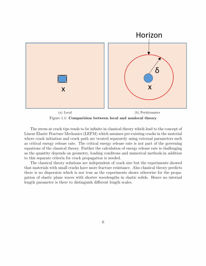
(a) Local (b) Peridynamics
Figure 1.1: Comparision between local and nonlocal theory
The stress at crack tips tends to be infinite in classical theory which lead to the concept ofLinear Elastic Fracture Mechanics (LEFM) which assumes pre-existing cracks in the materialwhere crack initiation and crack path are treated separately using external parameters suchas critical energy release rate. The critical energy release rate is not part of the governingequations of the classical theory. Further the calculation of energy release rate is challengingas the quantity depends on geometry, loading conditons and numerical methods.in additionto this separate criteria for crack propagation is needed.
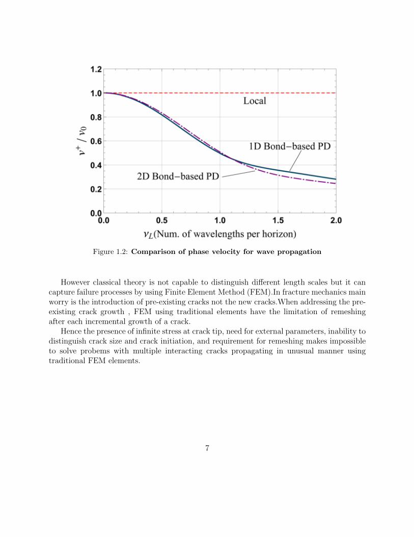
The classical theory solutions are independent of crack size but the experiments showedthat materials with small cracks have more fracture resistance. Also classical theory predictsthere is no dispersion which is not true as the experiments shows otherwise for the propa-gation of elastic plane waves with shorter wavelengths in elastic solids. Hence no internallength parameter is there to distinguish different length scales.
6
Figure 1.2: Comparison of phase velocity for wave propagation
However classical theory is not capable to distinguish different length scales but it cancapture failure processes by using Finite Element Method (FEM).In fracture mechanics mainworry is the introduction of pre-existing cracks not the new cracks.When addressing the pre-existing crack growth , FEM using traditional elements have the limitation of remeshingafter each incremental growth of a crack.
Hence the presence of infinite stress at crack tip, need for external parameters, inability todistinguish crack size and crack initiation, and requirement for remeshing makes impossibleto solve probems with multiple interacting cracks propagating in unusual manner usingtraditional FEM elements.
7
1.2 Basic Definitions
1.2.1 Equation of Motion
The peridynamic equation of motion of any particle X in reference configuration at time tis given as
ρ∂2u
∂t2=
∫R
f(u(X
′, t)− u(X, t),X
′ −X)dVX′ + b (X, t) (1.1)
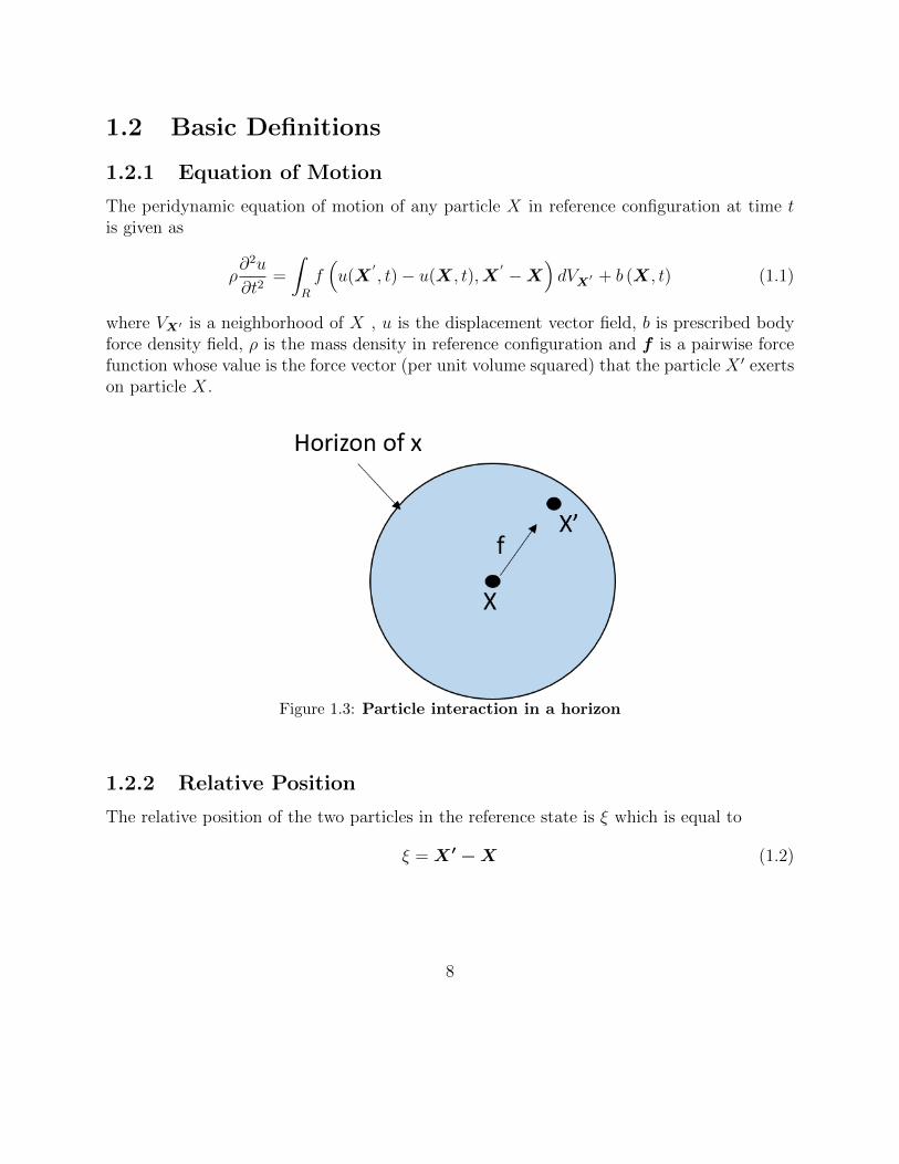
where VX′ is a neighborhood of X , u is the displacement vector field, b is prescribed bodyforce density field, ρ is the mass density in reference configuration and f is a pairwise forcefunction whose value is the force vector (per unit volume squared) that the particle X ′ exertson particle X.
Figure 1.3: Particle interaction in a horizon
1.2.2 Relative Position
The relative position of the two particles in the reference state is ξ which is equal to
ξ = X ′ −X (1.2)
8
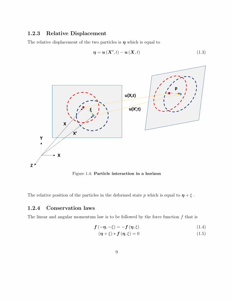
1.2.3 Relative Displacement
The relative displacement of the two particles is η which is equal to
η = u (X ′, t)− u (X, t) (1.3)
Figure 1.4: Particle interaction in a horizon
The relative position of the particles in the deformed state p which is equal to η + ξ .
1.2.4 Conservation laws
The linear and angular momentum law is to be followed by the force function f that is
f (−η,−ξ) = −f (η, ξ) (1.4)
(η + ξ) ∗ f (η, ξ) = 0 (1.5)
9
for all ξ,η. The above expressions implies that the relative position is parallel to the forcebetween the two particles. The general form of the bond force for the basic theory can bewritten as
f (η, ξ) =ξ + η
|ξ + η|f (p, ξ, t) (1.6)
where the scalar bond force is represented as f and also
p = |η + ξ|. (1.7)
1.2.5 Bond stretch
Like in classical theory , where there is a strain, here it is a scalar bond stretch ′s′b which isdefined as
sb =|ξ + η| − |η|
|ξ|(1.8)
For a brittle material to be microelastic, it should have
f (s, t, ξ) = χ (t, ξ) csb (1.9)
where χ is a history dependent damage function taking values of either 0 or 1 and c repre-senting spring constant
χ (t, ξ) = 1 if sb (t′, ξ) < so for all 0 ≤ t′ ≤ t (1.10)
= 0 otherwise (1.11)
where so is the critical bond stretch for failure which means if the bond stretch is hasexceeding critical bond stretch, the bond is assumed broken. The value of spring constantc is found by equating the energy density within the horizon in the peridynamic theory tostrain energy under isotropic extension from continuum mechanics for the same deformation.Thus
c =18K
πδ4(1.12)
where δ is the horizon. The critical stretch for bond failure , so is related to the energyrelease rate G as
so =
(10G
πcδ5
) 12
=
(5G
9Kδ
) 12
(1.13)
10
This is obtained by equating work done to break all bonds in a unit area to energy releaserate Silling and Askari (2005) described that introduction of failure at interaction level leadsto local damage at a point given by
1−∫Vχ (X, t, ξ) dVX∫VdVX
(1.14)
where R represents spherical volume with radius equal to horizon of δ and the centre ofsphere is at X. So we can get the definition of the local damage at a point as ratio ofamount of broken interactions to total amount of interactions .
1.3 Horizon size
Horizon of a material point refers to the region in which it has its influence on the othermaterial points i.e it can have interactions with other material points in that region only. Itis a length-scale parameter from which peridynamics gets its non-local behaviour.The typeof the problem and its nature defines the selection of the horizon size. If the problem isnot having any non-local behaviour,horizon should converge to zero In which case, classicalcontinuum theory and peridynamics are equivalent of each other.We use the numerical tech-niques to solve the problems in peridynamics.Using a very small value of horizon size , thecomputational time gets very large. So that size of horizon should be chosen which doesn’tshow any significant non-local character which we can get by doing some convergence study.In problems which have non-local and non-classical behaviour horizon is used as a lengthscale parameter which we can adjust according to the required physical behaviour that canbe correctly represented.In a beam where crack is to appear or loading is applied , we cannotchoose uniform size of horizon all over the beam, the region in which it is assumed for thecrack to appear and the loading, we can have a smaller horizon of each material point.Forthe problems in which the cross section area of the material is changing, we can use smallhorizon size to accurately detect the behaviour of material at the change of cross section.
1.4 Advantages and Limitations
� Advantages
– Offers potentially great generality in fracture modeling.
* Cracks nucleate and grow spontaneously.
* Cracks follow from the basic field equations.
11
– Any material model from local theory can be used.
– Compatible with molecular scale long-range forces.
– Length scale can be exploited for multiscale modeling.
� Limitations
– Slow due to many interactions.
– Need smarter integration methods.
– surface effects: correction methods are available but none totally satisfactory.
– boundary conditions are different from the local theory.
– Particle discretization has known limitations.
12
Chapter 2
LITERATURE REVIEW
The nonlocal peridynamic theory has been proven to be a promising method for modellingthe material failure and damage analysis in solid mechanics .The modelling of complexfracture problems such as crack branching and spontaneous crack nucleation and , curvingand arrest can be done easily using the integro differential equations of peridynamics. Ninget al. [2] studied the damage due to impact in a three point bending beam with offset notchusing the peridynamic approach which is widely used for the mixed I-II crack propagation inbrittle materials . The predictions from the peridynamic analysis agree well with availableexperimental observations. The numerical results show that the dynamic fracture behaviourof the beam under the impact load such as crack initiation, curving and branching rely on thelocation of offset notch and the impact speed of the drop hammer. It has been observed thatin modal response of an aluminium plate with clamped free boundary conditions, the naturalfrequencies from peridynamics agree better with the experimental results than the frequenciesfrom finite elements for all modes except mode I [3]. Differences between peridynamics andexperiment results ranged (in magnitude )from 0.13 to 10.38% and between pridynamic andfinite-elements from 0.23% to 9.72%. The non local peridynamic theory is applied to studythe structural vibration and impact damage using 2D bond based peridynamics and the thenumerical results indicate that the peridynamic solutions for beams vibration problems arealmost identical to the results based on Euler-Bernoulli beam theory. It is also found thatthe feature of softer material near the boundary in peridynamics has a notable effect on thesolution of beam vibration [4]. Gardy et al. [5] developed a new state based peridynamicmodel which is used to represent the bending of an Euler-Bernoulli beam. This model isfound to give accurate deformation results for simple beam tests. The perfect plasticity andsimple brittle damage models successfully reproduce the impact of non-linear behaviours ondeformation of rectangular cantilever and the framework is laid to allow application of thesame models to I-beams. This novel model simplifies treatment of bending in beams and
13
is extensible to bending in plates. Silling et al. [6] used PD theory for damage predictionconsidering Kalthoff-Winkler experiment [7], in which a plate having two parallel notchesis hit by impactor and peridynamic simulations successfully captured angle of crack growththat is observed in the experiments. This technique does not reqiure the specification ofkinetic laws for crack growth and because it does not require the tracking of individualcracks, it models fracture mechanics problems of arbitrary complexity with potentially greatgenerality. Silling and Askari [8] showed the convergence of peridynamics using a plate with acentre crack. Gardy et al. [9], using the peridynamic state based beam model, determined thebending of a Kirchoff-Love plate. This model is non ordinary and is derived from the conceptof a rotational spring between bonds. This simple extension of beam model reproduces platebending with a poisson ratio of 0.33, which can be combined with a 2D linear peridynamicsolid model to simulate mixed in-plane and transverse loading. Peridynamic theory can beapplied to fracture problems in contrast to the approach of fracture mechanics. By usingperidynamics, the crack path for inclined crack under dynamic loading were investigated.The peridynamics solution for this problem represents the main features of dynamic crackpropagation such as crack bifurcation. The problem is solved for various angles and differentstress values. The results are compared with molecular dynamic solutions that seem to showreasonable agreement in branching position and time [10]. High velocity impact and shockor blast responses are a critical design characteristic determing sizing of composite parts andultimately weight savings .Peridynamis can be used to accurately predict nonlinear transientdeformations and damage behaviour of compositess under shock or blast type of loadings dueto explosions .Peridynamics provide the ability to predict residual strength and durability forimproving structural designs of composites under such loadings[11]. Yile et al. [12] studiedthe delamination and the effect of fiber waviness using PD. It is shown that the simulationscorrectly perdicted the damage initiation and progression in the double cantilever beam(DCB) made up of laminated composite with wavy fibers. Jifeng et al. [13] et al. studieddelmination and matrix damage process in composite laminates due to low velocity impact,and the simulations showed that damage area correlates very well with the experimentaldata. The peridynamic formulation for a unidirectional fiber-reinforced composite laminabased on homogenization and mapping between elastic and fracture parameters of the micro-scale peridynamic bonds and the macro-scale parameters of the composite is developedby Wenke et al. [14]. The model is then used to analyze the splitting mode (mode II)fracture in dynamic loading of a 0◦ lamina. Appropriate scaling factors are used in themodel in order to have the elastic strain energy, for a fixed nonlocal interaction distance(the peridynamic horizon). Yozo et al. [15] developed a systematic analytical treatmentof peristatic and peridynamic problems for a 1D infinite rod. It is found from the studythat some peridynamic materials can have negative group velocities in certain regions ofwavenumber. This indicates that peridynamics can also be used for modeling certain types
14
of dispersive media with anomalous dispersion. Sarego et al.[16] developed a 2D linearizedordinary state-based peridynamic model. The convergence behavior of peridynamic solutionsin terms of the size of the nonlocal region by comparison with the classical (local) mechanicsmodel is also studied. The degree to which the peridynamic surface effect influences therecovery of elastic properties is examined, and stress/strain recovery values are found to havea definite influence on the results. The technique used here can provide the basis for applying2D peridynamic models to the study of fatigue failure and quasi-static fracture problems.The PD model developed by Le et al. [17] for plane stress and plane strain was studied andvalidated using a two dimensional rectangular plate with a round hole in the middle underconstant tensile stress. The model is found to show the m -convergence and δ - convergencebehaviors. The problem of cracks propagation in thin orthotropic flat plates under bendingloads was studied by Tastan et al. [18] using peridynamics. The formulation followed here isbased on the main ideas of bond based Peridynamics. Several numerical examples show thatthe results obtained with the new approach are in good agreement with those obtained withmore classical computational methods. Moreover the numerically computed crack patternsseem to follow in a reasonable way the orthotropic properties of the models . Michael etal.[19] developed a plate model as a two-dimensional approximation of the three-dimensionalbond-based theory of peridynamics via an asymptotic analysis. The resulting plate theoryis demonstrated using a specially designed peridynamics code to simulate the fracture of abrittle plate with a central crack under tensile loading.
15
Chapter 3
APPLICATION TO EULERBERNOULLI BEAM
Every object in the world has a 3-Dimensional geometrical shape and it is usually possible tomodel structures in a 3-Dimensional fashion although this approach can be computationallyexpensive. In order to reduce computational time, the 3-Dimensional geometry can be sim-plified as a beam, plate or shell type of structure depending on the geometry and loading.This simplification should also be accurately reflected in the formulation which is used forthe analysis. In this study, we want to develop Euler-Bernoulli beam formulation withinordinary-state based peridynamic framework. The equation of motion can be obtained byutilizing Euler-Lagrange equations. The accuracy of the formulation is validated by consid-ering various benchmark problems subjected to different loading and displacement/rotationboundary conditions.
3.1 Formulation
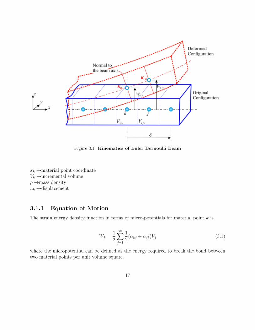
To represent an Euler Bernoulli Beam, we descretize the beam into single row of materialpoints. The descretization is meshless and the shape of the horizon is a line . Each ma-terial point is having only one degree of freedom that is transverse displacement along z-axis.
Consider two material points k and j with coordinates xk and xj and their transversedisplacements as uk and uj, with volume of horizon around each material point as Vk andVj respectively.After deformation, let κk andκj are their curvatures.
16
Figure 3.1: Kinematics of Euler Bernoulli Beam
xk →material point coordinateVk →incremental volumeρ→mass densityuk →displacement
3.1.1 Equation of Motion
The strain energy density function in terms of micro-potentials for material point k is
Wk =1
2
∞∑j=1
1
2(αkj + αjk)Vj (3.1)
where the micropotential can be defined as the energy required to break the bond betweentwo material points per unit volume square.
17
The micropotentials are also the functions of the transverse degree of freedom of thematerial points.
The PD equation of motion at material point xk is found out using principal of virtualwork which is
δ
∫ t1
to
(T − U)dt = 0 (3.2)
where T and U are the total kinetic and total potential energies of the systemTotal kinetic energy of the system is due to bending and transverse shear deformation totalpotential energy is obtained by the summation of micropotentials
Here u1j , u2j ,.. are the neighbourhood material points of j within the horizon.Similarly u1k , u2k ,.. are the neighbourhood material points of k within the horizon.Putting the value of lagrangian L from equation (3.7) in lagrangian equation
∂
∂t
(∂
∂uk
)− ∂L
∂uk= 0
(3.8)
ρkukVk +
(∞∑j=1
1
2
(∞∑i=1
∂αij∂(uj − ui)
Vi
)∂(uj − ui)
uk+∞∑j=1
1
2
(∑i=1
∂αik∂(uk − ui)
Vi
)∂(uk − ui)
uk− bk
)Vk = 0
or
ρkuk =∞∑j=1
1
2
(∞∑i=1
∂αki∂(ui − uk)
Vi
)−∞∑j=1
1
2
(∞∑i=1
∂αik∂(uk − ui)
Vi
)+ bk (3.9)
Using dimensional analysis, we come to know that the term∑∞
i=1
∂αki∂(uj − uk)
Vi represents
the force term.Let this term be the force density the material point xj exerts on xk. So the equation (3.9)can be written as
ρkuk =∞∑j=1
(tkj − tjk)Vj + bk (3.10)
19
where the tilde sign shows the force densities due to bending deformations
tkj =1
2Vj
∞∑i=1
∂αki∂(uj − uk)
Vi =1
Vj
∂(12
∑∞i=1 αkiVi
)∂(uj − uk)
Vi (3.11)
=1
Vj
∂Wk
∂(uj − uk)(3.12)
Using classical continuum mechanics, the strain energy density for material points k can berepresented as
Wk =1
2aκ2k (3.13)
where κk is curvature of material point k and a is peridynamic constantThe curvature for material point k can be defined as
κk = d∞∑ik
uik − ukξ2ikk
Vik (3.14)
where ik represents all material points inside the horizon of material point k and d is also aperidynamic constant
ξikk = |xk − xik | (3.15)
Putting the value of κk in eq.(3.13),we get
Wk =1
2ad2
(∞∑ik
uik − ukξ2ikk
Vik
)2
(3.16)
Putting value of Wk in equation (3.12) we get
tkj =ad2
Vik
(∞∑ik
uik − ukξ2ikk
Vik
)Vik
ξ2ikk
=adκkξ2jk
(3.17)
20
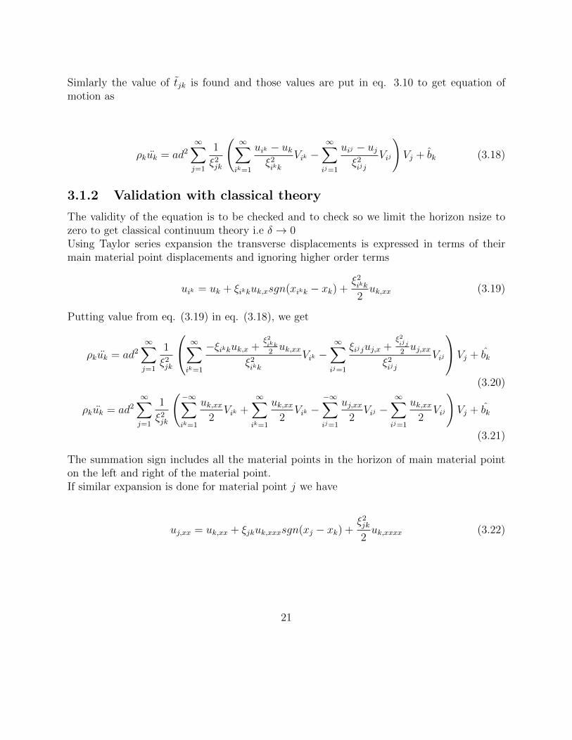
Simlarly the value of tjk is found and those values are put in eq. 3.10 to get equation ofmotion as
ρkuk = ad2∞∑j=1
1
ξ2jk
(∞∑ik=1
uik − ukξ2ikk
Vik −∞∑ij=1
uij − ujξ2ijj
Vij
)Vj + bk (3.18)
3.1.2 Validation with classical theory
The validity of the equation is to be checked and to check so we limit the horizon nsize tozero to get classical continuum theory i.e δ → 0Using Taylor series expansion the transverse displacements is expressed in terms of theirmain material point displacements and ignoring higher order terms
uik = uk + ξikkuk,xsgn(xikk − xk) +ξ2ikk
2uk,xx (3.19)
Putting value from eq. (3.19) in eq. (3.18), we get
ρkuk = ad2∞∑j=1
1
ξ2jk
∞∑ik=1
−ξikkuk,x +ξ2ikk
2uk,xx
ξ2ikk
Vik −∞∑ij=1
ξijjuj,x +ξ2ijj
2uj,xx
ξ2ijj
Vij
Vj + bk
(3.20)
ρkuk = ad2∞∑j=1
1
ξ2jk
(−∞∑ik=1
uk,xx2
Vik +∞∑ik=1
uk,xx2
Vik −−∞∑ij=1
uj,xx2
Vij −∞∑ij=1
uk,xx2
Vij
)Vj + bk
(3.21)
The summation sign includes all the material points in the horizon of main material pointon the left and right of the material point.If similar expansion is done for material point j we have
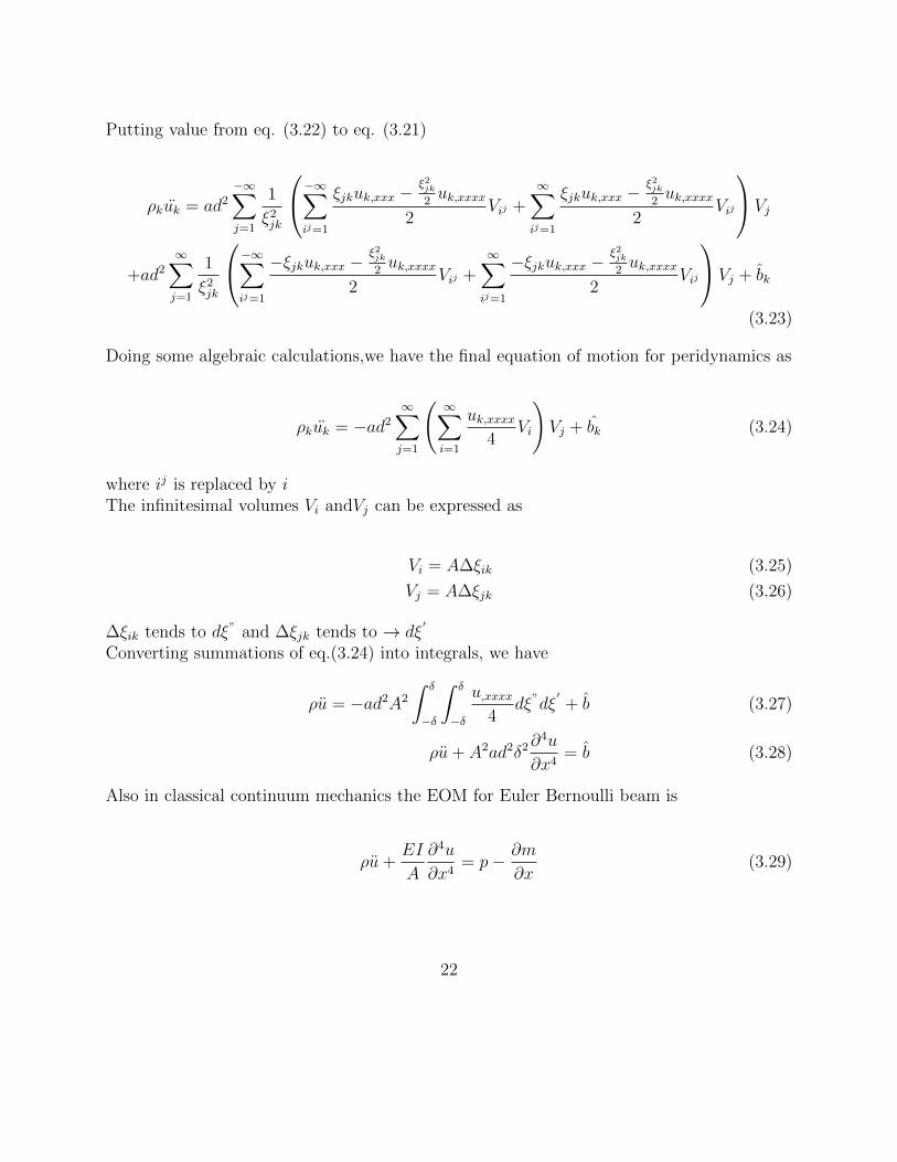
Doing some algebraic calculations,we have the final equation of motion for peridynamics as
ρkuk = −ad2∞∑j=1
(∞∑i=1
uk,xxxx4
Vi
)Vj + bk (3.24)
where ij is replaced by iThe infinitesimal volumes Vi andVj can be expressed as
Vi = A∆ξik (3.25)
Vj = A∆ξjk (3.26)
∆ξik tends to dξ” and ∆ξjk tends to → dξ′
Converting summations of eq.(3.24) into integrals, we have
ρu = −ad2A2
∫ δ
−δ
∫ δ
−δ
u,xxxx4
dξ”dξ′+ b (3.27)
ρu+ A2ad2δ2∂4u
∂x4= b (3.28)
Also in classical continuum mechanics the EOM for Euler Bernoulli beam is
ρu+EI
A
∂4u
∂x4= p− ∂m
∂x(3.29)
22
where p is the transverse load and∂m
∂xis the change in acting on a material volume.
Comparing eq. (3.28) and eq. (3.29) we get
a =EI
A3d2δ2(3.30)
b = p− ∂m
∂x(3.31)
We can calculate peridynamic material parameter d, by comparing the curvature of materialpoint in peridynamics with curvature in classical theory under a simple loading conditionwith constant curvature υ i.e
k = υ =∂2u
∂x2(3.32)
Integrating above equation, we get
ux =υx2
2+ ax+ b (3.33)
At x = δ and x = −δ , y=0.Satisfying these conditions we have
u =υx2
2− υδ2
2(3.34)
At x=0, uk = −υδ2
2
At x = ξ, uik = υξ2
2− υδ2
2
Putting the value of uik and uk in eq. 3.14 we get
κk = d∞∑ik=1
υ
2Vik (3.35)
κk = dυ
2
∫ δ
−δAdξ” (3.36)
κk = dυAδ (3.37)
Equating above value with υ we get
d =1
Aδ(3.38)
23
Putting the value of d in eq. (3.30)
a =EIA2δ2
A3δ2(3.39)
a =EI
A(3.40)
Putting the value of a in (3.13) we get
Wk =1
2
EI
Aκ2k (3.41)
which is same as the strain energy density function in the classical theory.
This shows that we can recover classical theory by reducing horizon size in peridynamicsto zero.
24
Chapter 4
APPLICATION TO TIMOSHENKOBEAM
Progressive failure analysis of structures is still a major challenge. There exist various predic-tive techniques to tackle this challenge by using both classical (local) and nonlocal theories.Peridynamic (PD) theory (nonlocal) is very suitable for this challenge, but computationallycostly with respect to the finite element method. When analyzing complex structures, it isnecessary to utilize structural idealizations to make the computations feasible. Therefore,this study presents the PD equations of motions for structural idealizations such as beamswhile accounting for transverse shear deformation. Also, their PD dispersion relations areto be presented and compared with those of classical theory .
4.1 Formulation
For a Timoshenko Beam also, we descretize the beam into single row of material points. Thedescretization is meshless and the shape of the horizon is a line . Each material point ishaving only one degree of freedom that is transverse displacement along z-axis.But alongwiththe transverse displacement we have the shear deformation also.
Consider two material points k and j with coordinates xk and xj and their transversedisplacements as uk and uj, shear deformation as ϕk and ϕj, out of plane rotations asθkand θj with volume of horizon around each material point as Vk and Vj respectively.Afterdeformation, let κk andκj are their curvatures.
25
Figure 4.1: Kinematics of Timoshenko Beam
ϑk, ϑjare transverse shear anglesuk, ujare out of plane deflectionsθk, θjare out of plane rotations
ϑj =uj − ukξjk
− θjsign (xj − xk) (4.1)
ϑk =uj − ukξjk
− θksign (xj − xk) (4.2)
Assuming ϑkj as the average tansverse shear deformation due to the interaction betweenmaterial points j and k
ϑkj =uj − ukξjk
− θj + θk2
sign(xj − xk) (4.3)
Let κkj is curvature between material points j and k
κkj =θj − θkξjk
(4.4)
26
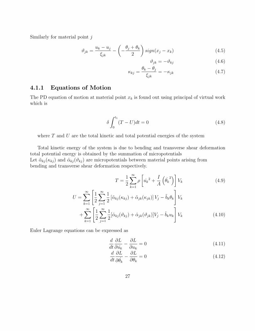
Similarly for material point j
ϑjk =uk − ujξjk
−(−θj + θk
2
)sign(xj − xk) (4.5)
ϑjk = −ϑkj (4.6)
κkj =θk − θjξjk
= −κjk (4.7)
4.1.1 Equations of Motion
The PD equation of motion at material point xk is found out using principal of virtual workwhich is
δ
∫ t1
0
(T − U)dt = 0 (4.8)
where T and U are the total kinetic and total potential energies of the system
Total kinetic energy of the system is due to bending and transverse shear deformationtotal potential energy is obtained by the summation of micropotentialsLet αkj(κkj) and αkj(ϑkj) are micropotentials between material points arising frombending and transverse shear deformation respectively.
T =1
2
∞∑k=1
ρ
[uk
2 +I
A
(θk
2)]
Vk (4.9)
U =∞∑k=1
[1
2
∞∑j=1
1
2[αkj(κkj) + αjk(κjk)]Vj − bkθk
]Vk
+∞∑k=1
[1
2
∞∑j=1
1
2[αkj(ϑkj) + αjk(ϑjk)]Vj − bkuk
]Vk (4.10)
Euler Lagrange equations can be expressed as
d
dt
∂L
∂uk− ∂L
∂uk= 0 (4.11)
d
dt
∂L
∂θk− ∂L
∂θk= 0 (4.12)
27
where
L = T − U (4.13)
T = · · ·+ 1
2ρuk
2Vk +1
2ρI
Aθk
2Vk + · · · (4.14)
−1
2
∞∑j=1
[1
2[αkj(κkj) + αjk(κjk)]Vj
]Vk · · ·
−1
2
∞∑j=1
[1
2[αkj(ϑkj) + αjk(ϑjk)]Vj
]Vk · · ·
−1
2
∞∑j=1
[1
2[αkj(κkj) + αjk(κjk)]Vj
]Vk · · ·
−1
2
∞∑j=1
[1
2[αkj(ϑkj) + αjk(ϑjk)]Vj
]Vk · · ·
+bkθkVk + bkukVk (4.15)
L = · · ·+ 1
2ρuk
2Vk +1
2ρI
Aθk
2Vk + · · ·
−∞∑j=1
[1
2[αkj(κkj) + αjk(κjk)]Vj
]Vk · · ·
−∞∑j=1
[1
2[αkj(ϑkj) + αjk(ϑjk)]Vj
]Vk · · ·
+bkθkVk + bkukVk (4.16)
Putting this L in the Lagrange equation, we get
ρukVk +∞∑j=1
[1
2
[∂αkj(ϑkj)
∂ϑkj
∂ϑkj∂uk
+∂αjk(ϑjk)
∂ϑjk
∂ϑjk∂uk
]Vj
]Vk − bkVk = 0 (4.17)
Let
1
ξjk
∂αkj(ϑkj)
∂ϑkj= fkj (4.18)
1
ξjk
∂αjk(ϑjk)
∂ϑjk= fjk (4.19)
28
Then we have
ρukVk +∞∑j=1
1
2
[ξjkfkj
∂ϑjk∂uk
+ ξjkfjk∂ϑjk∂uk
]Vj − bk = 0 (4.20)
Also
ρI
Aθk +
∞∑j=1
[1
2
[∂αkj(κkj)
∂κkj
∂κjk∂θk
+∂αjk(κjk)
∂κjk
∂κjk∂θk
]Vj
]Vk
+∞∑j=1
[1
2
[∂αkj(ϑkj)
∂ϑkj
∂ϑkj∂θk
+∂αjk(ϑjk)
∂ϑjk
∂ϑjk∂θk
]Vj
]Vk − bkVk = 0 (4.21)
Let
1
ξjk
∂αkj(κkj)
∂κkj= fkj (4.22)
1
ξjk
∂αjk(κjk)
∂κjk= fjk (4.23)
Then we have
ρI
Aθk +
∞∑j=1
1
2ξjk
[fkj
∂κkj∂θk
+ fjk∂κjk∂θk
]Vj
+∞∑j=1
1
2ξjk
[fkj
∂ϑkj∂θk
+ fjk∂ϑjk∂θk
]Vj − bk = 0 (4.24)
where fkj, fjkfkj, fjk, are peridynamic interaction forces between material points j and karising from bending and transverse shear deformation .
For linear behaviour, the interaction forces can also be defined as
fkj = cb(κkj) fjk = cb(κjk) (4.25)
fkj = cs(ϑkj) fjk = cs(ϑjk)
The peridynamic parameter associated with bending and transverse shear deformation arecs, cb
29
Putting these values of peridynamic forces and corresponding shear angles and curvaturesin EOM we have
ρuk = cs
∞∑j=1
(uj − ukξjk
− θj + θk2
sign(xj − xk))Vj + bk (4.26)
ρI
Aθk = cb
∞∑j=1
θj − θkξjk
Vj +1
2cs
∞∑j=1
(uj − ukξjk
− θj + θk2
sign(xj − xk))Vj + bk (4.27)
4.1.2 Validation with classical theory
Using Taylor series expansion we can express out of plane rotation and transverse sheardeformation at material point j as
uj = uk + uk,xξjksign(xj − xk) +1
2uk,xxξ
2jk (4.28)
θj = θk + θk,xξjksign(xj − xk) +1
2θk,xxξ
2jk (4.29)
Putting these values in the EOM gives
ρuk = cs
∞∑j=1
(uk + uk,xξjksign(xj − xk) + 1
2uk,xxξ
2jk − uk
ξjk
)
−cs∞∑j=1
(θk + θk,xξjksign(xj − xk) + 1
2θk,xxξ
2jk + θk
2sign(xj − xk)
)Vj + bk
= cs
∞∑j=1
(0 +
uk,xxξjk2
−(θksign(xj − xk) +
θk,xξjk(1− 0)
2+θk,xx
2ξ2jksign(xj − xk)
))Vj + bk
= cs
∞∑j=1
(uk,xxξjk
2− θk,xξjk
2
)Vj + bk
ρuk = cs
∞∑j=1
(uk,xx − θk,x)ξjkVj + bk
(4.30)
Similarly
ρI
Aθk = cb
∞∑j=1
θk,xxξjkVj + cs
∞∑j=1
(uk,x − θk −
1
4θk,xxξ
2jk
)Vj + bk (4.31)
30
Let Vj = A∆ξjk where ∆ξjkis representing the spacing between two consecutive materialpoints and replace summation by integration as ∆ξjk approaches zero. Now we have
ρu = cs
∫ δ
0
(u,xx − θ,x)ξAdξ + b
ρu = cs(u,xx − θ,x)Aδ2
2+ b (4.32)
Also
ρI
Aθ = cb
∫ δ
0
θ,xxξAdξ + cs
∫ δ
0
(u,x − θ −
1
4θ,xxξ
2
)ξAdξ + b
= cbδ2
2θ,xxA+
(u,x
δ2
2− θδ
2
2− θ,xxδ
4
16
)A+ b
ρI
Aθ =
Aδ2
2
(cb − cs
δ2
8
)θ,xx +
Aδ2
2cs(u,x − θ) + b (4.33)
The above PD equations have same form as classical Timoschenko Beam equations
ρu = kG(u,xx + θ,x) + b
ρI
Aθ =
EI
Aθ,xx + kG(u,x − θ)b (4.34)
Comparing coefficients we get the peridynamic material parameters as
cs =2kG
Aδ2cb = 2EI
δ2A2 + 14kGA
(4.35)
31
Chapter 5
APPLICATION TO MICROPOLARBEAM
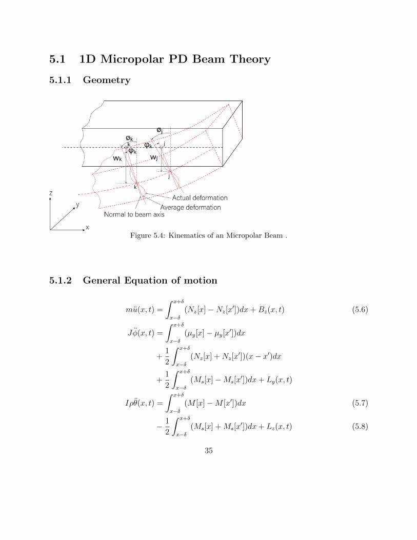
In micropolar continuum, it is assumed that there is a microstructre which can rotate inde-pendently from the surroundings. This means every particle contains six degrees of freedom, three translational motions which are assigned to macro element and three rotational oneswhich are assigned to the microstructure. In this method , in addition to force, particles ap-ply moments to each other that is if a particle rotates, the other particles will apply momentto that particle to resist deformation.
At each particle of a micropolar continuum, it is assumed that there is a microstructurewhich can rotate independently from the surrounding medium.
32
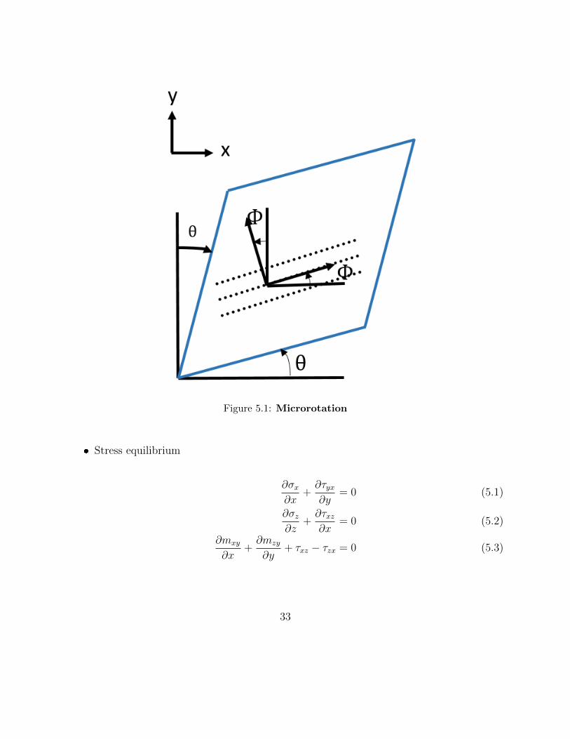
Figure 5.1: Microrotation
� Stress equilibrium
∂σx∂x
+∂τyx∂y
= 0 (5.1)
∂σz∂z
+∂τxz∂x
= 0 (5.2)
∂mxy
∂x+∂mzy
∂y+ τxz − τzx = 0 (5.3)
33
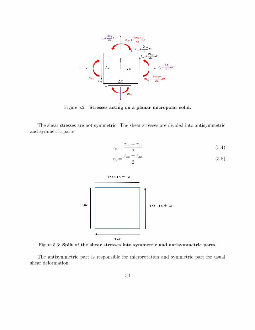
Figure 5.2: Stresses acting on a planar micropolar solid.
The shear stresses are not symmetric. The shear stresses are divided into antisymmetricand symmetric parts
τs =τxz + τzx
2(5.4)
τa =τxz − τzx
2(5.5)
Figure 5.3: Split of the shear stresses into symmetric and antisymmetric parts.
The antisymmetric part is responsible for microrotation and symmetric part for usualshear deformation.
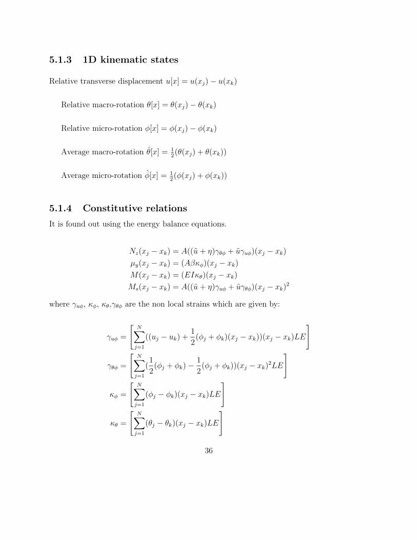
where γuφ, κφ, κθ,γθφ are the non local strains which are given by:
γuφ =
[N∑j=1
((uj − uk) +1
2(φj + φk)(xj − xk))(xj − xk)LE
]
γθφ =
[N∑j=1
(1
2(φj + φk)−
1
2(φj + φk))(xj − xk)2LE
]
κφ =
[N∑j=1
(φj − φk)(xj − xk)LE
]
κθ =
[N∑j=1
(θj − θk)(xj − xk)LE
]
36
5.1.5 Equation of motion
Putting the corresponding values in the equations (33), (34), (35), we get EOM as
mu(xk, t) = 2V (LE)N∑l=1
(ξjk)((µ+ η)N∑j=1
1
2(φj + φk)(ξjk)
2
+ µN∑j=1
(uj − uk)(ξjk)− ηN∑j=1
1
2(φj + φk)(ξjk)
2) (5.9)
Iρθ(xk, t) =N∑l=1
2EIξjk(LE)2N∑j=1
(θj − θk)(xj − xk)
− 1
2(2V (LE)
N∑l=1
(ξjk)2((µ+ η)
N∑j=1
(uj − uk)(ξjk)
+ µN∑j=1
1
2(θj + θk)(ξjk)
2 + ηN∑j=1
1
2(φj + φk)(ξjk)
2) (5.10)
Jφ(xk, t) = 2V LEβN∑l=1
ξjk
N∑j=1
(φj − φk)ξjk
− V (LE)ηN∑l=1
(ξjk)2(
N∑j=1
1
2(θj
+ θk)(ξjk)2 +
N∑j=1
(uj − uk)(ξjk))
+ 2V (LE)ηN∑l=1
(ξjk)2
N∑j=1
1
2(φj + φk)(ξjk)
2 (5.11)
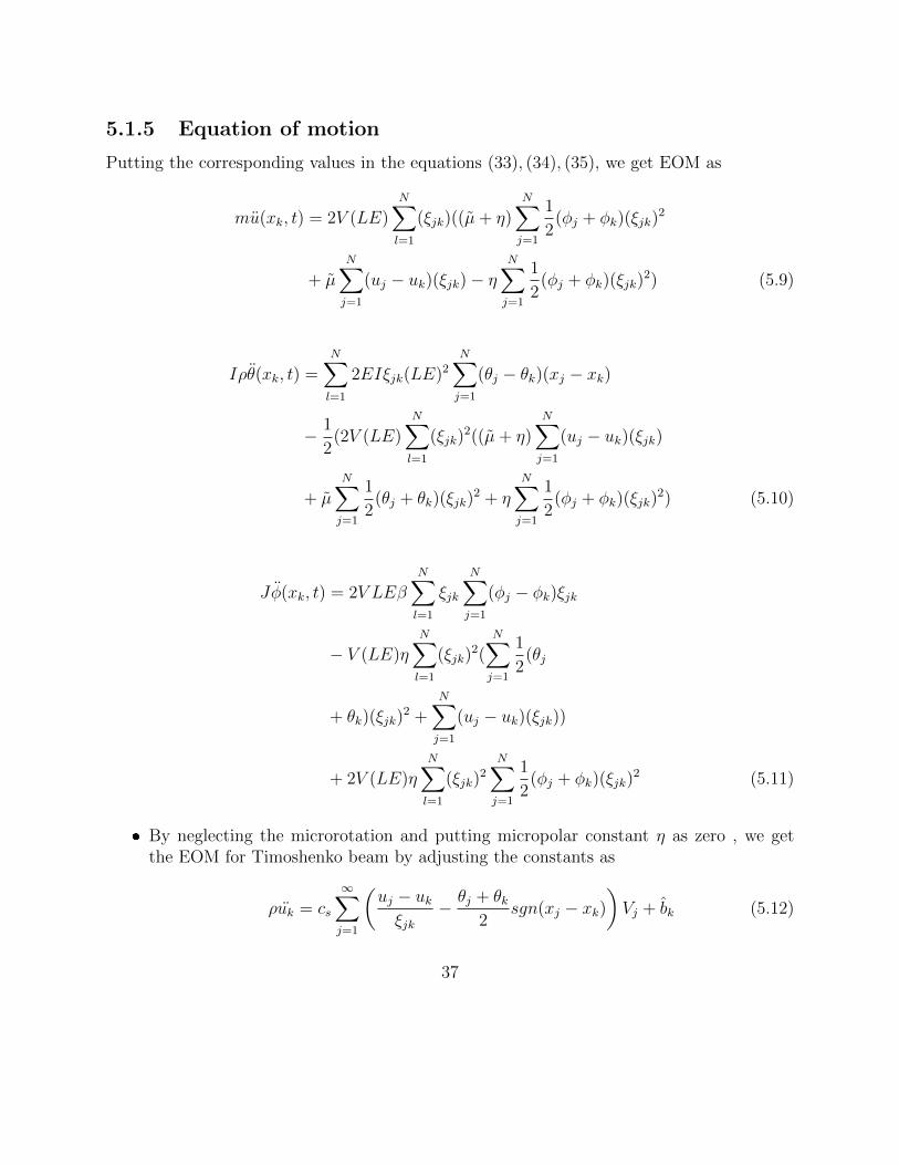
� By neglecting the microrotation and putting micropolar constant η as zero , we getthe EOM for Timoshenko beam by adjusting the constants as
ρuk = cs
∞∑j=1
(uj − ukξjk
− θj + θk2
sgn(xj − xk))Vj + bk (5.12)
37
ρI
Aθk =
cb
∞∑j=1
θj − θkξjk
Vj +1
2cs
∞∑j=1
(uj − ukξjk
sgn(xj − xk)−θj + θk
2
)ξjkVj + bk (5.13)
� Further neglecting the shear deformation and adjusting the constants, we get EOM forEuler Bernoulli beam as
ρkuk = ad2∞∑j=1
1
ξ2jk
(∞∑ik=1
uik − ukξ2ikk
Vik −∞∑ij=1
uij − ujξ2ijj
Vij
)Vj + bk (5.14)
38
Chapter 6
PROBLEM STATEMENT
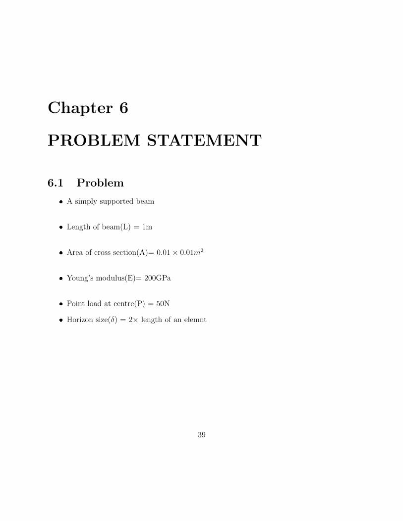
6.1 Problem
� A simply supported beam
� Length of beam(L) = 1m
� Area of cross section(A)= 0.01× 0.01m2
� Young’s modulus(E)= 200GPa
� Point load at centre(P) = 50N
� Horizon size(δ) = 2× length of an elemnt
39
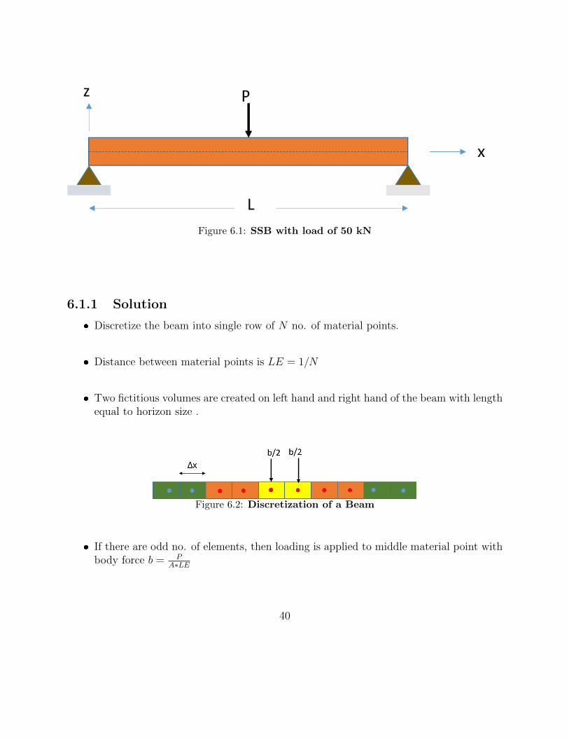
Figure 6.1: SSB with load of 50 kN
6.1.1 Solution
� Discretize the beam into single row of N no. of material points.
� Distance between material points is LE = 1/N
� Two fictitious volumes are created on left hand and right hand of the beam with lengthequal to horizon size .
Figure 6.2: Discretization of a Beam
� If there are odd no. of elements, then loading is applied to middle material point withbody force b = P
A∗LE
40
� If there are even no. of elements, then loading is applied to two middle material pointswith body force b = P
2∗A∗LE on each of the two material point.
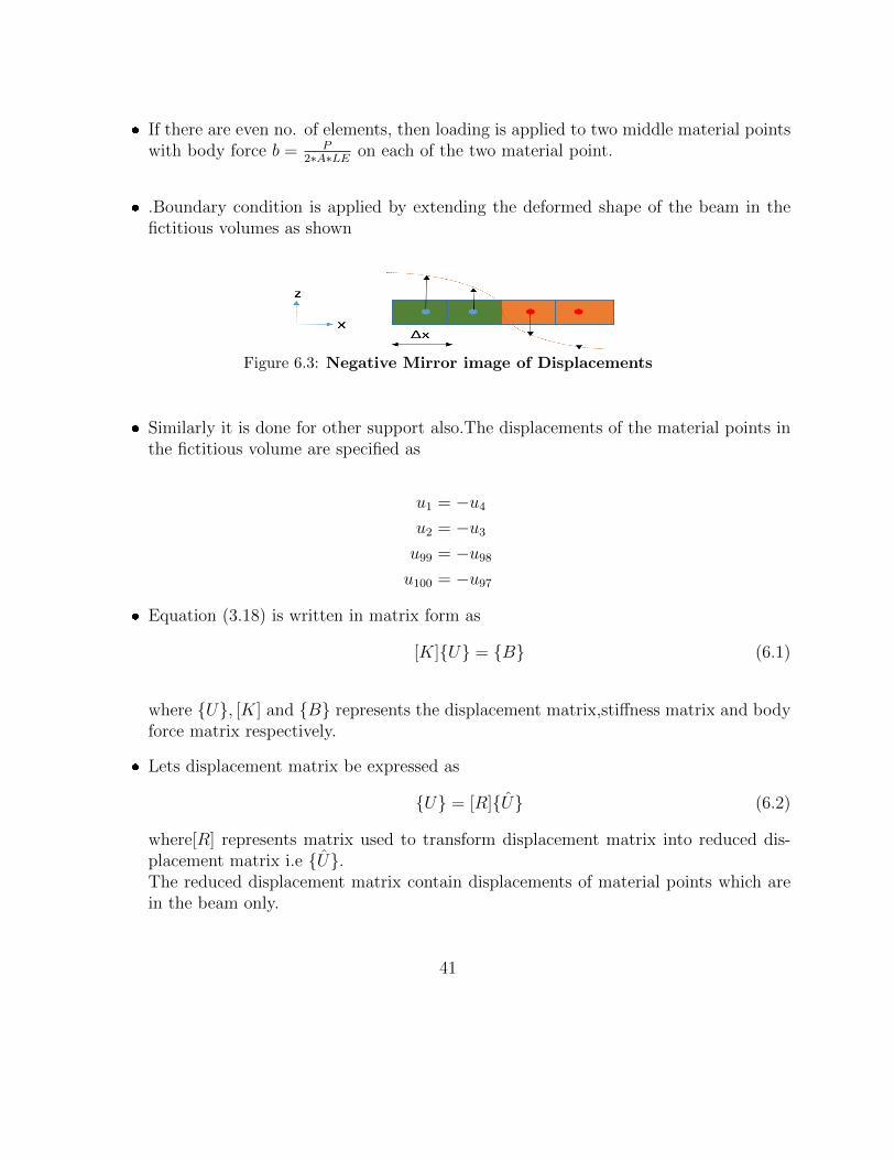
� .Boundary condition is applied by extending the deformed shape of the beam in thefictitious volumes as shown
Figure 6.3: Negative Mirror image of Displacements
� Similarly it is done for other support also.The displacements of the material points inthe fictitious volume are specified as
u1 = −u4u2 = −u3u99 = −u98u100 = −u97
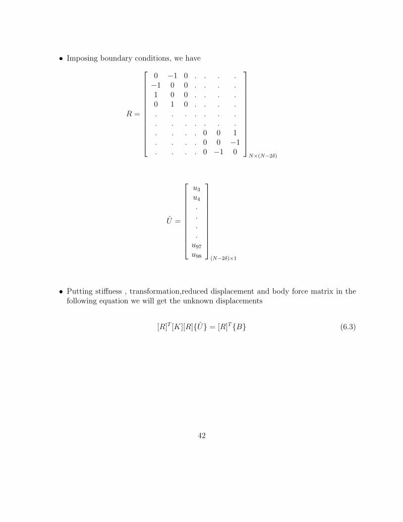
� Equation (3.18) is written in matrix form as
[K]{U} = {B} (6.1)
where {U}, [K] and {B} represents the displacement matrix,stiffness matrix and bodyforce matrix respectively.
� Lets displacement matrix be expressed as
{U} = [R]{U} (6.2)
where[R] represents matrix used to transform displacement matrix into reduced dis-placement matrix i.e {U}.The reduced displacement matrix contain displacements of material points which arein the beam only.
� Putting stiffness , transformation,reduced displacement and body force matrix in thefollowing equation we will get the unknown displacements
[R]T [K][R]{U} = [R]T{B} (6.3)
42
Chapter 7
RESULTS AND DISCUSSIONS
7.1 Euler Bernoulli Beam
7.1.1 Simply Supported Beam
0 0.1 0.2 0.3 0.4 0.5 0.6 0.7 0.8 0.9 1
Location (m)
-7
-6
-5
-4
-3
-2
-1
0
Tra
nsv
erse
dis
pla
cem
ent
(m)
10-3
NE= 50NE= 100NE= 200NE= 400NE= 800analytical
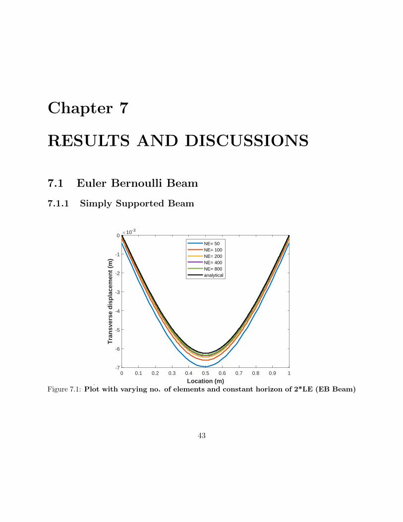
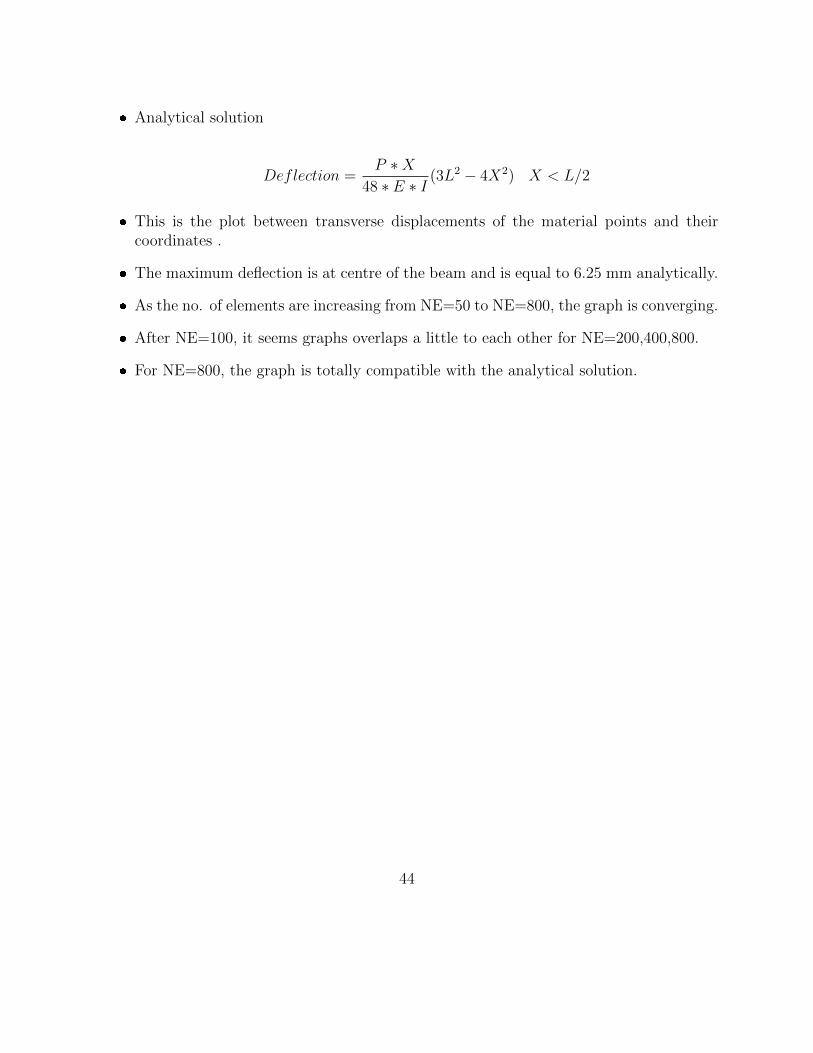
Figure 7.1: Plot with varying no. of elements and constant horizon of 2*LE (EB Beam)
43
� Analytical solution
Deflection =P ∗X
48 ∗ E ∗ I(3L2 − 4X2) X < L/2
� This is the plot between transverse displacements of the material points and theircoordinates .
� The maximum deflection is at centre of the beam and is equal to 6.25 mm analytically.
� As the no. of elements are increasing from NE=50 to NE=800, the graph is converging.
� After NE=100, it seems graphs overlaps a little to each other for NE=200,400,800.
� For NE=800, the graph is totally compatible with the analytical solution.
44
0 0.1 0.2 0.3 0.4 0.5 0.6 0.7 0.8 0.9 1
Location (m)
-7
-6
-5
-4
-3
-2
-1
0T
ran
sver
se d
isp
lace
men
t (m
)10-3
h= LEh= 2 LEh= 4 LEh= 6 LEh= 10 LEanalytical
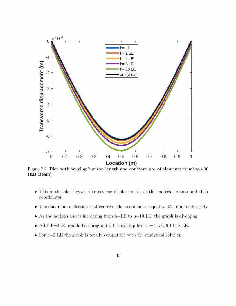
Figure 7.2: Plot with varying horizon length and constant no. of elements equal to 500(EB Beam)
� This is the plot beyween transverse displacements of the material points and theircoordinates .
� The maximum deflection is at centre of the beam and is equal to 6.25 mm analytically.
� As the horizon size is increasing from h=LE to h=10 LE, the graph is diverging
� After h=2LE, graph discourages itself to overlap from h=4 LE, 6 LE, 8 LE.
� For h=2 LE the graph is totally compatible with the analytical solution.
45
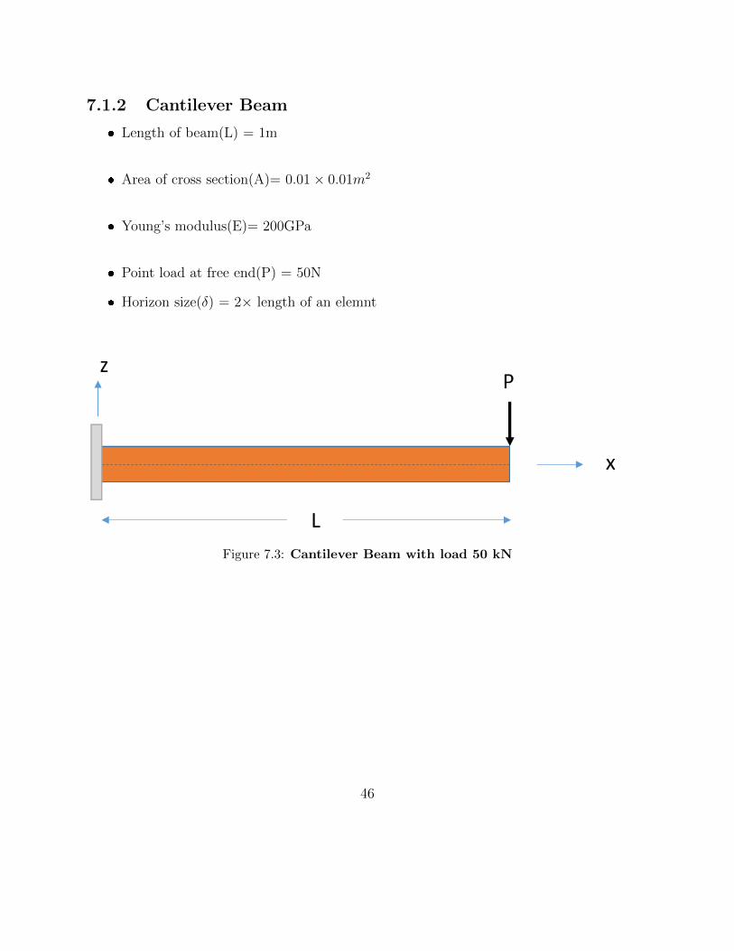
7.1.2 Cantilever Beam
� Length of beam(L) = 1m
� Area of cross section(A)= 0.01× 0.01m2
� Young’s modulus(E)= 200GPa
� Point load at free end(P) = 50N
� Horizon size(δ) = 2× length of an elemnt
Figure 7.3: Cantilever Beam with load 50 kN
46
0 0.1 0.2 0.3 0.4 0.5 0.6 0.7 0.8 0.9 1
Location (m)
-0.11
-0.1
-0.09
-0.08
-0.07
-0.06
-0.05
-0.04
-0.03
-0.02
-0.01
Tra
nsv
erse
dis
pla
cem
ent
(m)
NE=50NE=100NE=200NE=400NE=800analytical
Figure 7.4: Plot with varying no. of elements and constant horizon of 2*LE (EB Beam)
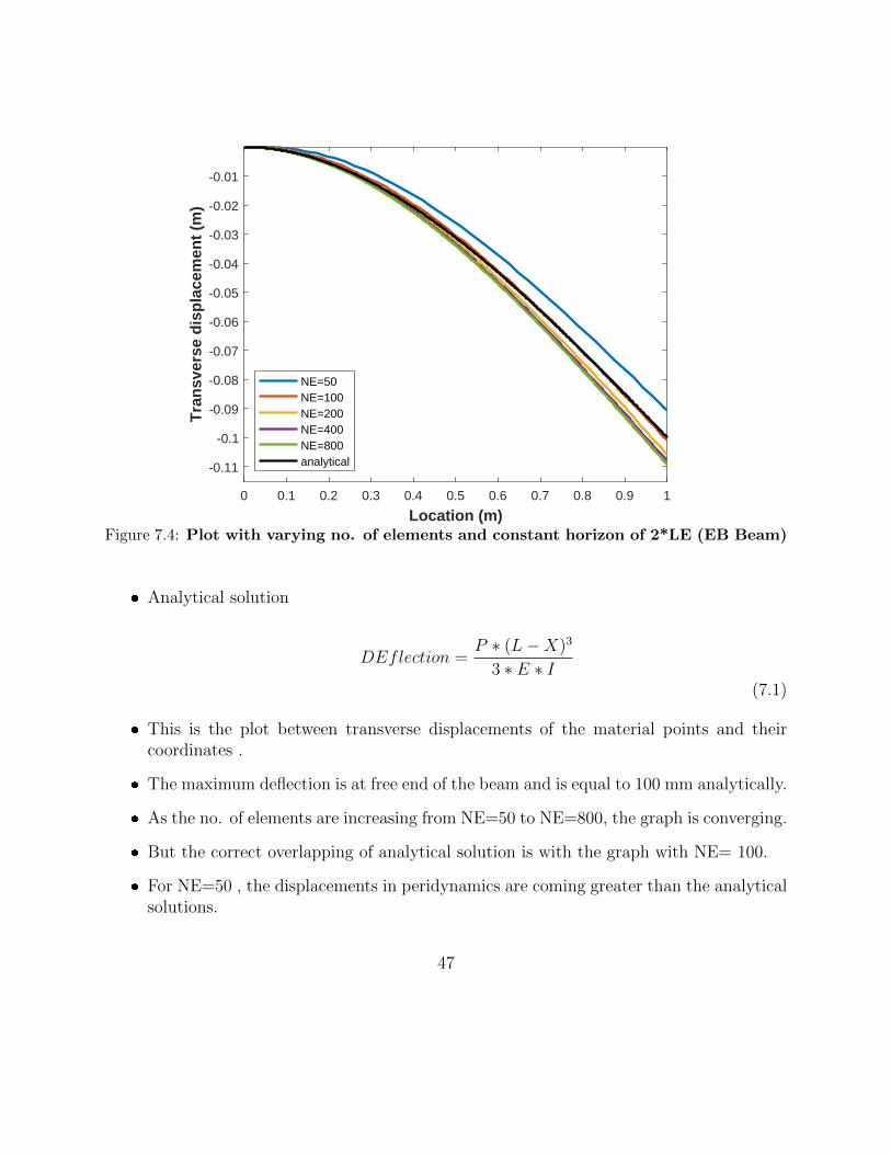
� Analytical solution
DEflection =P ∗ (L−X)3
3 ∗ E ∗ I(7.1)
� This is the plot between transverse displacements of the material points and theircoordinates .
� The maximum deflection is at free end of the beam and is equal to 100 mm analytically.
� As the no. of elements are increasing from NE=50 to NE=800, the graph is converging.
� But the correct overlapping of analytical solution is with the graph with NE= 100.
� For NE=50 , the displacements in peridynamics are coming greater than the analyticalsolutions.
47
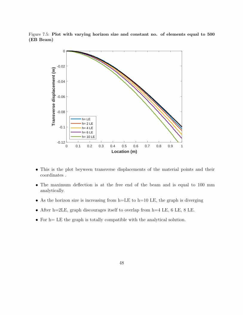
Figure 7.5: Plot with varying horizon size and constant no. of elements equal to 500(EB Beam)
0 0.1 0.2 0.3 0.4 0.5 0.6 0.7 0.8 0.9 1
Location (m)
-0.12
-0.1
-0.08
-0.06
-0.04
-0.02
0T
ran
sver
se d
isp
lace
men
t (m
)
h= LEh= 2 LEh= 4 LEh= 6 LEh= 10 LE
� This is the plot beyween transverse displacements of the material points and theircoordinates .
� The maximum deflection is at the free end of the beam and is equal to 100 mmanalytically.
� As the horizon size is increasing from h=LE to h=10 LE, the graph is diverging
� After h=2LE, graph discourages itself to overlap from h=4 LE, 6 LE, 8 LE.
� For h= LE the graph is totally compatible with the analytical solution.
48
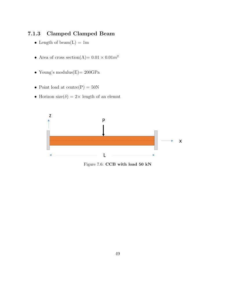
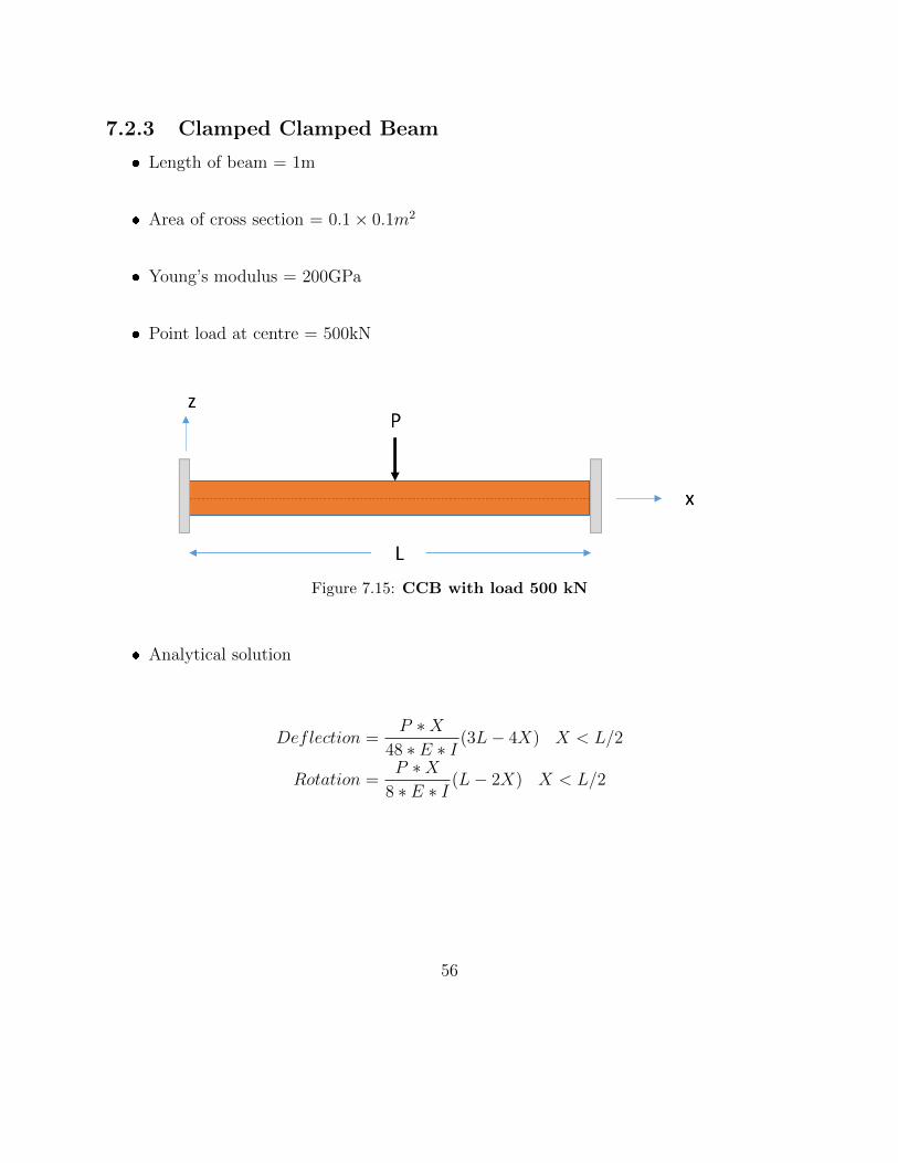
7.1.3 Clamped Clamped Beam
� Length of beam(L) = 1m
� Area of cross section(A)= 0.01× 0.01m2
� Young’s modulus(E)= 200GPa
� Point load at centre(P) = 50N
� Horizon size(δ) = 2× length of an elemnt
Figure 7.6: CCB with load 50 kN
49
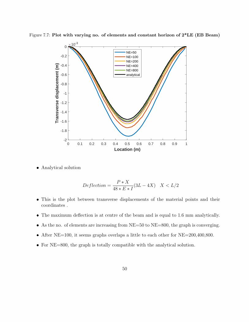
Figure 7.7: Plot with varying no. of elements and constant horizon of 2*LE (EB Beam)
0 0.1 0.2 0.3 0.4 0.5 0.6 0.7 0.8 0.9 1
Location (m)
-2
-1.8
-1.6
-1.4
-1.2
-1
-0.8
-0.6
-0.4
-0.2
0
Tra
nsv
erse
dis
pla
cem
ent
(m)
10-3
NE=50NE=100NE=200NE=400NE=800analytical
� Analytical solution
Deflection =P ∗X
48 ∗ E ∗ I(3L− 4X) X < L/2
� This is the plot between transverse displacements of the material points and theircoordinates .
� The maximum deflection is at centre of the beam and is equal to 1.6 mm analytically.
� As the no. of elements are increasing from NE=50 to NE=800, the graph is converging.
� After NE=100, it seems graphs overlaps a little to each other for NE=200,400,800.
� For NE=800, the graph is totally compatible with the analytical solution.
50
0 0.1 0.2 0.3 0.4 0.5 0.6 0.7 0.8 0.9 1
Location (m)
-1.8
-1.6
-1.4
-1.2
-1
-0.8
-0.6
-0.4
-0.2
0
Tra
nsv
erse
dis
pla
cem
ent
(m)
10-3
h= LEh= 2 LEh= 4 LEh= 6 LEh= 10 LEanalytical
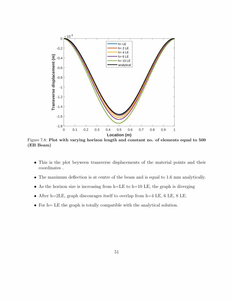
Figure 7.8: Plot with varying horizon length and constant no. of elements equal to 500(EB Beam)
� This is the plot beyween transverse displacements of the material points and theircoordinates .
� The maximum deflection is at centre of the beam and is equal to 1.6 mm analytically.
� As the horizon size is increasing from h=LE to h=10 LE, the graph is diverging
� After h=2LE, graph discourages itself to overlap from h=4 LE, 6 LE, 8 LE.
� For h= LE the graph is totally compatible with the analytical solution.
51
7.2 Timoshenko Beam
7.2.1 Simply Supported Beam
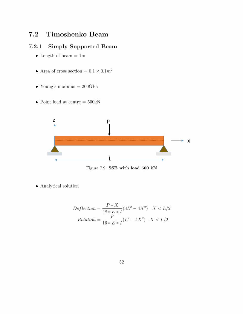
� Length of beam = 1m
� Area of cross section = 0.1× 0.1m2
� Young’s modulus = 200GPa
� Point load at centre = 500kN
Figure 7.9: SSB with load 500 kN
� Analytical solution
Deflection =P ∗X
48 ∗ E ∗ I(3L2 − 4X2) X < L/2
Rotation =P
16 ∗ E ∗ I(L2 − 4X2) X < L/2
52
0 0.1 0.2 0.3 0.4 0.5 0.6 0.7 0.8 0.9 1
Location (m)
-7
-6
-5
-4
-3
-2
-1
0T
ran
sver
se d
isp
lace
men
t (m
)10-3
NE= 50NE= 100NE= 200NE= 400NE= 800analytical
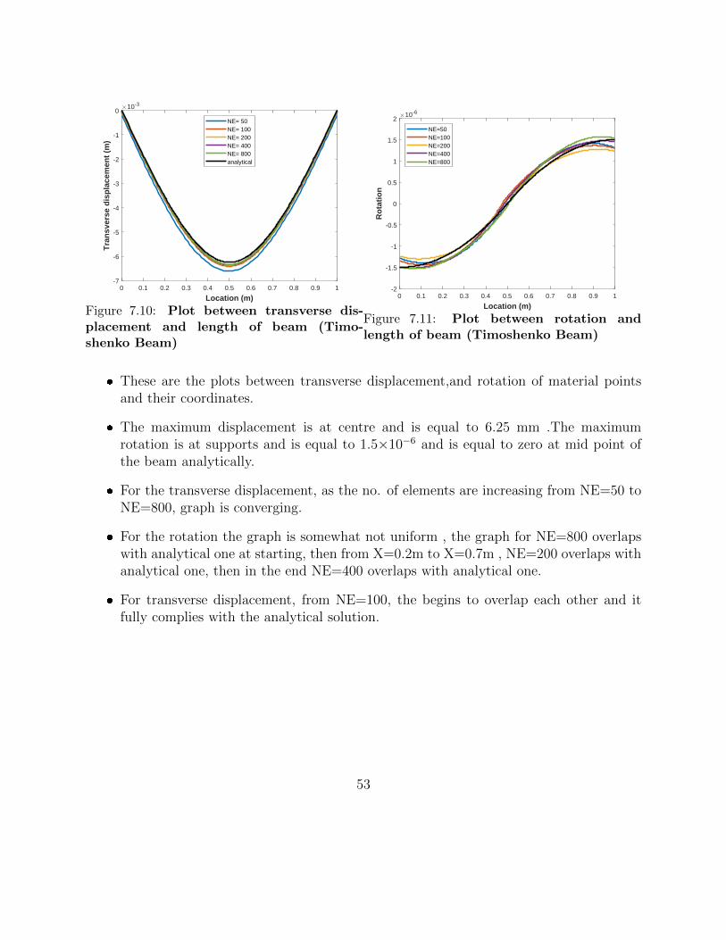
Figure 7.10: Plot between transverse dis-placement and length of beam (Timo-shenko Beam)
0 0.1 0.2 0.3 0.4 0.5 0.6 0.7 0.8 0.9 1
Location (m)
-2
-1.5
-1
-0.5
0
0.5
1
1.5
2
Ro
tati
on
10-6
NE=50NE=100NE=200NE=400NE=800
Figure 7.11: Plot between rotation andlength of beam (Timoshenko Beam)
� These are the plots between transverse displacement,and rotation of material pointsand their coordinates.
� The maximum displacement is at centre and is equal to 6.25 mm .The maximumrotation is at supports and is equal to 1.5×10⁻⁶ and is equal to zero at mid point ofthe beam analytically.
� For the transverse displacement, as the no. of elements are increasing from NE=50 toNE=800, graph is converging.
� For the rotation the graph is somewhat not uniform , the graph for NE=800 overlapswith analytical one at starting, then from X=0.2m to X=0.7m , NE=200 overlaps withanalytical one, then in the end NE=400 overlaps with analytical one.
� For transverse displacement, from NE=100, the begins to overlap each other and itfully complies with the analytical solution.
53
7.2.2 Cantilever Beam
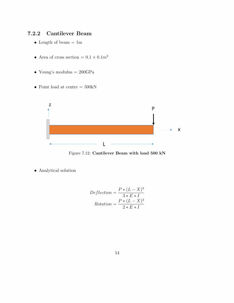
� Length of beam = 1m
� Area of cross section = 0.1× 0.1m2
� Young’s modulus = 200GPa
� Point load at centre = 500kN
Figure 7.12: Cantilever Beam with load 500 kN
� Analytical solution
Deflection =P ∗ (L−X)3
3 ∗ E ∗ I
Rotation =P ∗ (L−X)2
2 ∗ E ∗ I
54
0 0.1 0.2 0.3 0.4 0.5 0.6 0.7 0.8 0.9 1
Location (m)
-0.1
-0.09
-0.08
-0.07
-0.06
-0.05
-0.04
-0.03
-0.02
-0.01
0
Tra
nsv
erse
Dis
pla
cem
ent
(m)
NE=50NE=100NE=200NE=400NE=800analytical
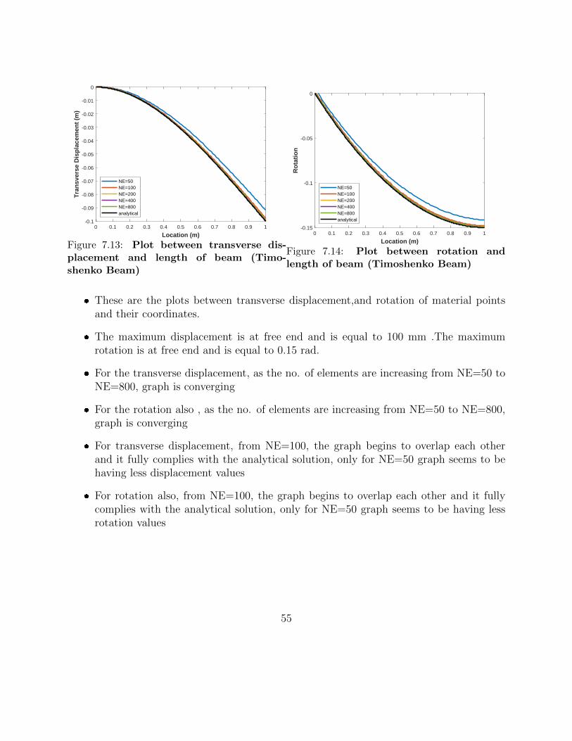
Figure 7.13: Plot between transverse dis-placement and length of beam (Timo-shenko Beam)
0 0.1 0.2 0.3 0.4 0.5 0.6 0.7 0.8 0.9 1
Location (m)
-0.15
-0.1
-0.05
0
Ro
tati
on
NE=50NE=100NE=200NE=400NE=800analytical
Figure 7.14: Plot between rotation andlength of beam (Timoshenko Beam)
� These are the plots between transverse displacement,and rotation of material pointsand their coordinates.
� The maximum displacement is at free end and is equal to 100 mm .The maximumrotation is at free end and is equal to 0.15 rad.
� For the transverse displacement, as the no. of elements are increasing from NE=50 toNE=800, graph is converging
� For the rotation also , as the no. of elements are increasing from NE=50 to NE=800,graph is converging
� For transverse displacement, from NE=100, the graph begins to overlap each otherand it fully complies with the analytical solution, only for NE=50 graph seems to behaving less displacement values
� For rotation also, from NE=100, the graph begins to overlap each other and it fullycomplies with the analytical solution, only for NE=50 graph seems to be having lessrotation values
55
7.2.3 Clamped Clamped Beam
� Length of beam = 1m
� Area of cross section = 0.1× 0.1m2
� Young’s modulus = 200GPa
� Point load at centre = 500kN
Figure 7.15: CCB with load 500 kN
� Analytical solution
Deflection =P ∗X
48 ∗ E ∗ I(3L− 4X) X < L/2
Rotation =P ∗X
8 ∗ E ∗ I(L− 2X) X < L/2
56
0 0.1 0.2 0.3 0.4 0.5 0.6 0.7 0.8 0.9 1
Location (m)
-1.6
-1.4
-1.2
-1
-0.8
-0.6
-0.4
-0.2
0
Tra
nsv
erse
dis
pla
cem
ent
(m)
10-3
NE=50NE=100NE=200NE=400NE=800analytical
Figure 7.16: Plot between transverse dis-placement and length of beam (Timo-shenko Beam)
0 0.1 0.2 0.3 0.4 0.5 0.6 0.7 0.8 0.9 1
Location (m)
-5
-4
-3
-2
-1
0
1
2
3
4
5
Ro
tati
on
10-3
NE=50NE=100NE=200NE=400NE=800analytical
Figure 7.17: Plot between rotation andlength of beam (Timoshenko Beam)
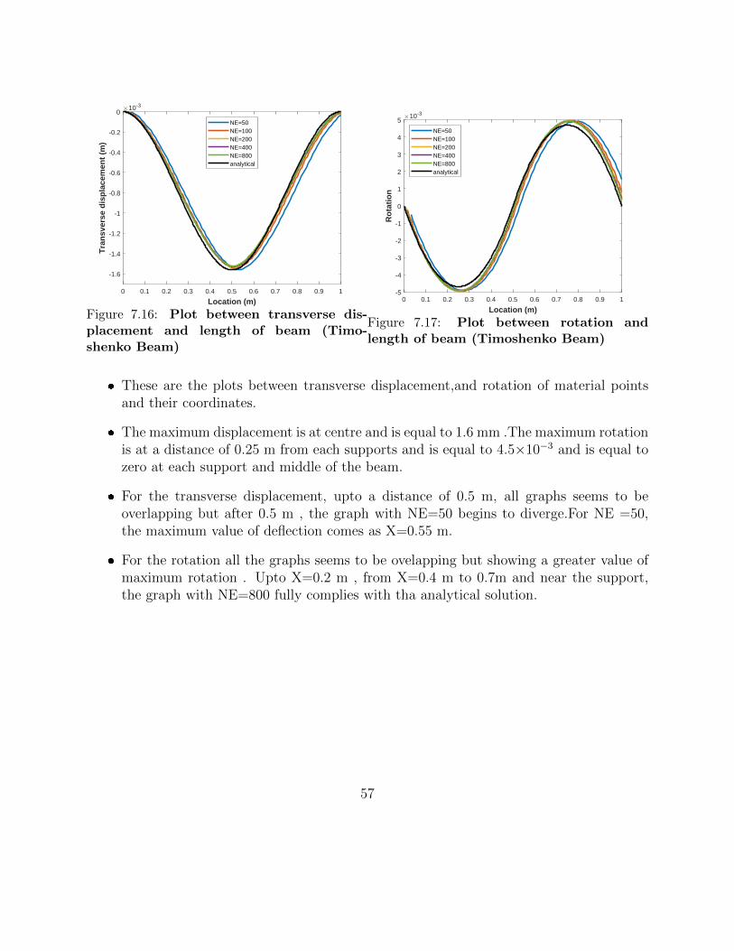
� These are the plots between transverse displacement,and rotation of material pointsand their coordinates.
� The maximum displacement is at centre and is equal to 1.6 mm .The maximum rotationis at a distance of 0.25 m from each supports and is equal to 4.5×10⁻³ and is equal tozero at each support and middle of the beam.
� For the transverse displacement, upto a distance of 0.5 m, all graphs seems to beoverlapping but after 0.5 m , the graph with NE=50 begins to diverge.For NE =50,the maximum value of deflection comes as X=0.55 m.
� For the rotation all the graphs seems to be ovelapping but showing a greater value ofmaximum rotation . Upto X=0.2 m , from X=0.4 m to 0.7m and near the support,the graph with NE=800 fully complies with tha analytical solution.
57
Chapter 8
SCOPE OF PRESENT WORK
– PRODUCTION SOFTWARE
* Unify Peridigm/Sierra/EMU
* Address usability and interface issues
* Material model library
– SOLVERS AND NUMERICAL METHODS
* SPH, kernel methods connection
* Next gen platforms
* Eulerian and ALE capability
– MATERIAL/DAMAGE MODELING
* Ductile failure
* continuum damage mechanics
* Quasistatic material failure
* Digital Image correlation (DIC)
* Nonlocal deformation measures
– MULTISCALE
* Scalable multiscale methods
* Coarse graining
* Atomistic-to-continuum coupling
* General tool for material failure
– MATH AND THEORY
58
* Quantify uncertainty specially in fracture
* Contact algorithms
* Material stability
– MULTIPHYSICS
* Math and numeric for multiphysics
* Geological applications
* Fluid-structure interaction
* Diffusion, chemical reactions
* Electromagnetic fields
* Electronics and MEMS reliability
* Friction
59
Bibliography
[1] Francesco dell’Isola, Ugo Andreaus, and Luca Placidi. A still topical contribution ofGabrio Piola to Continuum Mechanics: the creation of peridynamics, nonlocal andhigher gradient continuum mechanics. 2014.
[2] Ning Liu and Dahsin Liu. Peridynamic modeling of impact damage in 3 point bendingbeam with offset notch. Applied Mathematics and Mechanics, 38:99–110, 2017.
[3] A Freimanis and A Paegltis. Modal analysis of isotropic beams in peridynamics. IOPConference Series: Materials Science and Engineering, 251:1–7, 2017.
[4] B.O Chen, Ning Liu, and Guolai Yang. Application of peridynamics in predicting beamvibration and impact damage. Journal of Vibro Enineering, 21:2369–2378, 2015.
[5] James O’ Gardy and John Foster. Peridynamic beams: A non-ordinary, state-basedmodel. International Journal of Solids and Structures, 51:3177–3183, 2014.
[6] S A Silling. Reformulation of elasticity theory for discontinuities and long range forces.Journal of Mechanics and Physics of Solids, 48:175–209, 2000.
[7] J F Kalthoff and S Winkler. Failure mode transition at high rates of shear loading.Impact Loading and Dynamic Behaviour of Materials, 1:185–195, 1988.
[8] S . A. Siling and E. Askari. A meshfree method based on the peridynamic model ofsolid mechanics. Computers and Structures, 83:1526–1535, 2004.
[9] James O’ Gardy and John Foster. Peridynamic plates and flat shells:a non ordinarystate based model. International Journal of Solids and Structures, 51:4572–4579, 2014.
[10] A Shafei. Dynamic crack propagation in plates weakened by inclined cracks :investiga-tion based on periynamics. Frontiers of structural and civil engineering, 12, 2018.
[11] C Diyaroglu, E Oterkus, E Madenci, T Rabczuk, and A Siddiq. Peridynamic modelingof composites laminates under explosion. Composite Structures, 144, 2016.
60
[12] Yile Hu, Erdogan Madenci, and Nam Phan. Peridynamic modeling of defects in com-posites. Structural Dynamics and Materials Conference, 2015.
[13] Jifeng Xu, Abe Askari, Olaf Wreckner, and Stewart Silling. Peridynmic analysis ofimpact damage in composite laminates. Journal of Aerospace Engineering, 21:23–42,2008.
[14] Wenke Hu, Youn Doh Ha, and Florin Babaru. Modeling dynamic fracture and dam-age in a fiber reinforced composite lamina with peridynamics. Journal for MultiscaleComputational Engineering,, 9:707–726, 2011.
[15] Yozo Mikata. Analytical solution of peristatic and peridynamics problems for a 1Dinfinite rod. International Journal of Solids and Structures, 49:2887–2897, 2012.
[16] G. Sarego, Q. V. Le, F. Bobaru, M. Zaccariotto, and U. Galvanetto. Linearized statebased peridynamics for 2D problems. International Journal for Numerical methods inEngineering, 108:1174–1197, 2016.
[17] Q.V. Le, W.K. Chan, and J. Schwartz. A 2D ordinary state based peridynamic modelfor linearly elastic solids. International journal for numeriacal methods in engineering,98(4):547–561, 2014.
[18] A.Tastan, U.Yoluma, M.A.Guleran M.Zaccariotto, and U.Galvanetto. A 2D peridy-namic model for failure analysis of orthotropic thin plates due to bending. ProcediaStructural Integrity, 2:261–268, 2016.
[19] Michael Taylor and David J Steigmann. A 2 D peridynamic model for thin plates.Mathematics and Mechanics of solids, 2013.