Peridynamic Theory of Solid Mechanics S. A. Silling * R. B. Lehoucq † Sandia National Laboratories Albuquerque, New Mexico 87185-1322 USA April 28, 2010 Dedicated to the memory of James K. Knowles Contents 1 Introduction 4 1.1 Purpose of the peridynamic theory ............... 4 1.2 Summary of the literature .................... 5 1.3 Organization of this article ................... 11 2 Balance laws 13 2.1 Balance of linear momentum .................. 13 2.2 Principle of virtual work ..................... 18 2.3 Balance of angular momentum ................. 19 2.4 Balance of energy ......................... 21 2.5 Master balance law ........................ 24 3 Peridynamic states: notation and properties 28 4 Constitutive modeling 32 4.1 Simple materials ......................... 32 4.2 Kinematics of deformation states ................ 34 4.3 Directional decomposition of a force state ........... 34 4.4 Examples ............................. 35 * Multiscale Dynamic Material Modeling Department, [email protected]† Applied Mathematics and Applications Department, [email protected]1
Transcript
Peridynamic Theory of Solid Mechanics
S. A. Silling∗
R. B. Lehoucq†
Sandia National LaboratoriesAlbuquerque, New Mexico 87185-1322 USA
April 28, 2010
Dedicated to the memory of James K. Knowles
Contents
1 Introduction 41.1 Purpose of the peridynamic theory . . . . . . . . . . . . . . . 41.2 Summary of the literature . . . . . . . . . . . . . . . . . . . . 51.3 Organization of this article . . . . . . . . . . . . . . . . . . . 11
The peridynamic theory of mechanics attempts to unite the mathematicalmodeling of continuous media, cracks, and particles within a single frame-work. It does this by replacing the partial differential equations of the clas-sical theory of solid mechanics with integral or integro-differential equations.These equations are based on a model of internal forces within a body inwhich material points interact with each other directly over finite distances.
The classical theory of solid mechanics is based on the assumption ofa continuous distribution of mass within a body. It further assumes thatall internal forces are contact forces [73] that act across zero distance. Themathematical description of a solid that follows from these assumptionsrelies on partial differential equations that additionally assume sufficientsmoothness of the deformation for the PDEs to make sense in either theirstrong or weak forms. The classical theory has been demonstrated to pro-vide a good approximation to the response of real materials down to smalllength scales, particularly in single crystals, provided these assumptions aremet [52]. Nevertheless, technology increasingly involves the design and fab-rication of devices at smaller and smaller length scales, even interatomicdimensions. Therefore, it is worthwhile to investigate whether the classi-cal theory can be extended to permit relaxed assumptions of continuity, toinclude the modeling of discrete particles such as atoms, and to allow theexplicit modeling of nonlocal forces that are known to strongly influence thebehavior of real materials.
Similar considerations apply to cracks and other discontinuities: thePDEs of the classical theory do not apply directly on a crack or dislocationbecause the deformation is discontinuous on these features. Consequently,the techniques of fracture mechanics introduce relations that are extraneousto the basic field equations of the classical theory. For example, linear elas-tic fracture mechanics (LEFM) considers a crack to evolve according to aseparate constitutive model that predicts, on the basis of nearby conditions,how fast a crack grows, in what direction, whether it should arrest, branch,and so on. Although the methods of fracture mechanics provide importantand reliable tools in many applications, it is uncertain to what extent thisapproach can meet the future needs of fracture modeling in complex mediaunder general conditions, particularly at small length scales. Similar con-siderations apply to certain methods in dislocation dynamics, in which themotion of a dislocation is determined by a supplemental relation.
Aside from requiring these supplemental constitutive equations for thegrowth of defects within LEFM and dislocation dynamics, the classical the-ory predicts some well-known nonphysical features in the vicinity of these
4
singularities. The unbounded stresses and energy densities predicted by theclassical PDEs are conventionally treated in idealized cases by assuming thattheir effect is confined to a small process zone near the crack tip or withinthe core of a dislocation [38]. However, the reasoning behind neglecting thesingularities in this way becomes more troublesome as conditions and ge-ometries become more complex. For example, it is not clear that the energywithin the core of a dislocation is unchanged when it moves near or acrossgrain boundaries. Any such change in core energy could affect the drivingforce on a dislocation.
Molecular dynamics (MD) provides an approach to understanding themechanics of materials at the smallest length scales that has met with im-portant successes in recent years. However, even with the fastest computers,it is widely recognized that MD cannot model systems of sufficient size tomake it a viable replacement for continuum modeling.
These considerations motivate the development of the peridynamic the-ory, which attempts to treat the evolution of discontinuities according to thesame field equations as for continuous deformation. The peridynamic theoryalso has the goal of treating discrete particles according to the same fieldequations as for continuous media. The ability to treat both the nanoscaleand macroscale within the same mathematical system may make the methodan attractive framework in which to develop multiscale and atomistic-to-continuum methods.
1.2 Summary of the literature
The term “peridynamic” first appeared in [60] and comes from the Greekroots for near and force. The model proposed in [60] treats internal forceswithin a continuous solid as a network of pair interactions similar to springs.In this respect it is similar to Navier’s theory of solids (see Section 6). Inthe peridynamic model, the springs can be nonlinear. The responses of thesprings can depend on their direction in the reference configuration, leadingto anisotropy, and on their length. The maximum distance across which apair of material points can interact through a spring is called the horizon,because a given point cannot “see” past its horizon. The horizon is treatedas a constant material property in [60]. The equation of motion proposedin the original peridynamic theory is
ρ(x)u(x, t) =∫H
f(u(x′, t)− u(x, t),x′ − x
)dVx′ + b(x, t) (1)
where x is the position vector in the reference configuration of the body B,ρ is density, u is displacement, and b is a prescribed body force density. His a neighborhood of x with radius δ, where δ is the horizon for the mate-rial. Constitutive modeling, as proposed in [60], consists of prescribing the
5
pairwise force function f(η, ξ) for all bonds ξ = x′ − x and for all relativedisplacements between the bond endpoints, η = u′ − u. f can depend non-linearly on η, and there is no assumption that the bond forces are zero in thereference configuration. f has dimensions of force/volume2. Linearization ofthe equation of motion results in an expression that is formally the same asin Kunin’s nonlocal theory [46, 47] although constitutive modeling and otheraspects are different; a comparison between the two models is discussed inSection 6.5.
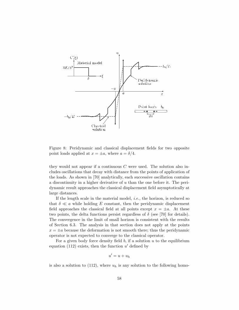
A number of papers have investigated various aspects of the linear peri-dynamic theory. In [70], the static loading by a body force density of aninfinitely long, homogeneous bar is considered. The resulting solutions, ob-tained using Fourier transforms, demonstrate interesting features not presentin solutions of the classical equilibrium equation. Among these are oscilla-tions that decay at points far from where the loading is applied, a resultof the nonlocality in the equations. (The physical significance of these fea-tures is not yet clear.) Dispersion curves are derived from isotropic materialmodels in [60], along with a variational formulation and some aspects ofmaterial stability. Zimmermann [83] explored many features of theory, in-cluding certain aspects of wave motion, material stability, and numericalsolution techniques. Zimmermann also studied energy balance for crackgrowth within the theory.
Weckner and Abeyaratne [75] studied the dynamics of a one dimensionalbar and obtained a Green’s function representation of the solution. Theyalso derived expressions for the evolution of discontinuities in the displace-ment field. Stable discontinuities (i.e., discontinuities that do not grow un-boundedly over time) can occur for certain choices of the initial data, evenwith well-behaved material properties. For other materials, discontinuitiescan grow unboundedly over time, leading to a type of material instability.Green’s functions for three dimensional unbounded elastic isotropic mediawere derived in [77] for both statics and dynamics. This work also presenteda comparison between the local and peridynamic theories for linear elasticsolids.
Alali and Lipton [3], Du and Zhou [18, 19], and Emmrich and Weck-ner [20, 21] establish various existence and uniqueness results for the linearperidynamic balance of momentum. These papers also draw equivalenceswith the weak solution of the classical equations of linear elasticity, andshow, in a precise sense, the well-posedness of the peridynamic equationsin the limit as the nonlocality vanishes. In particular, the limiting solutioncoincides with the conventional weak solution given sufficient regularity ofthe boundary data and material properties. Within the context of nonlocalsteady-state diffusion, Gunzburger and Lehoucq [35] introduce a nonlocalGauss’s theorem and nonlocal Green identities to establish well-posedness
6
of the nonlocal boundary value problem.The peridynamic theory as outlined in [60] suffers from significant restric-
tions on the scope of material behavior that can be modeled, in particularthe Poisson ratio is always 1/4 for isotropic materials. This motivated arethinking of the whole peridynamic theory. The outcome was a conceptwhich preserves the idea of bonds carrying forces between pairs of particles.However, in the new approach, the forces within each bond are not deter-mined independently of each other. Instead, each bond force depends on thecollective deformation (and possibly the rate of deformation and history) ofall the bonds within the horizon of each endpoint. The resulting modifiedtheory is called state-based, because the mathematical objects that conveyinformation about the collective deformation of bonds are called peridynamicstates (see Section 3). The technical discussion in the present article dealsprimarily with the state-based theory, although the earlier bond-based theoryis shown to be a special case of this. The state-based theory is discussed ingreater detail in [67], which includes a specific isotropic solid material modelin which any Poisson ratio can be prescribed.
It is also shown in [67] that any elastic constitutive model from theclassical theory can be adapted to the peridynamic theory using a nonlo-cal approximation to the deformation gradient tensor. Application of thistechnique to a strain-hardening plasticity model is demonstrated in [74, 27].The stress tensor provided by the classical constitutive model is mappedonto the bond forces in a way consistent with the approximation used forthe deformation gradient (see Section 4.11).
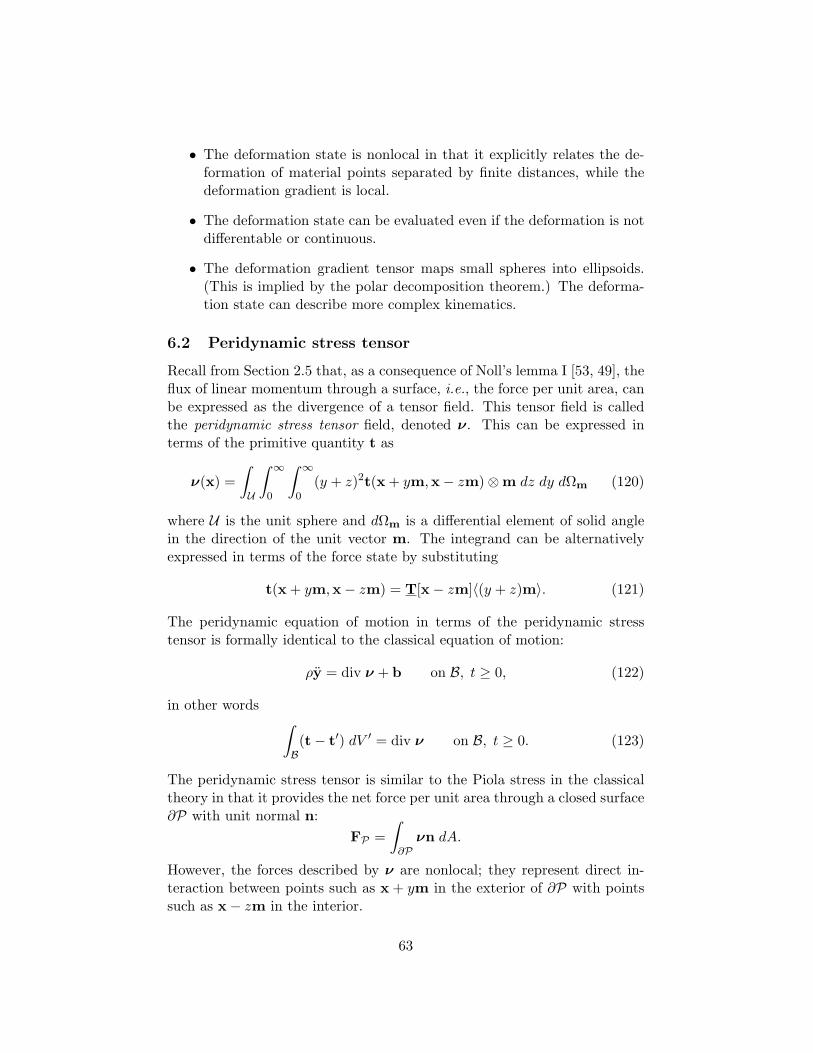
A peridynamic stress tensor (see Section 6.2) was derived in [48], al-though a similar concept was previously discussed in [83]. The peridynamicstress tensor has a mechanical interpretation similar to the Piola stress ten-sor in the classical theory. It provides the force per unit area across anyimaginary internal surface. However, in the peridynamic case, the stresstensor is nonlocal: the forces involved are the nonlocal forces in bonds thatcross from one side of the surface to the other. The peridynamic operator forthe internal force density can be expressed exactly as the divergence of theperidynamic stress tensor field. Thus, the peridynamic equation of motionbecomes formally the same as the classical equation.
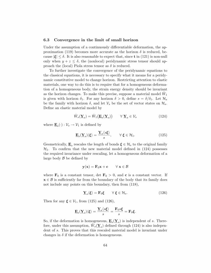
The convergence of the bond-based peridynamic theory to the equationsof classical elasticity theory was demonstrated by Zimmermann [83], and inthe context of isotropic linear elastic solids by Emmrich and Weckner [21].Within the state-based framework for constitutive modeling, it was shown in[68] that if a deformation is classically smooth, then the peridynamic oper-ator for internal force density approaches the classical operator in the limitof small horizon (see Section 6.3). The limiting process produces a classi-cal constitutive model for Piola stress as a limiting case of the peridynamic
7
stress for small horizon. In this sense, the peridynamic theory converges tothe classical theory.
Sears and Lehoucq [58] provide a statistical mechanical foundation forthe peridynamic balance of linear momentum. The nonlocality of force in-teraction is intrinsic and originates in molecular force interaction that isnonlocal. This analysis is similar to the landmark work of Irving and Kirk-wood [39], who had the objective of deriving the classical, rather than peri-dynamic, field equations from statistical physics. The classical balance oflinear momentum is a consequence of the more general peridynamic balancewhen the integral operator is expressed as the divergence of a stress tensor.In the important special case of a pair-potential, Noll [58, 49] in effect de-rives the peridynamic balance of linear momentum as an intermediate stepin deriving the classical balance from the principles of statistical mechanics.
Gerstle et al. extended the peridynamic mechanics model to diffusiveprocesses including heat conduction and migration of species due to highelectrical current density [31]. They applied the combined nonlocal equa-tions incorporating multiple physical mechanisms, including species diffu-sion, heat transport, mechanics, and electrical conduction, to a model prob-lem demonstrating the failure of an electronic component due to electromi-gration.
Nearly all of the applications of the peridynamic model to date rely onnumerical solutions. A numerical technique for approximating the peridy-namic field equations was proposed in [61]. This numerical method simplyreplaces the volume integral in (1) with a finite sum:
ρih2
(un+1i − 2uni + un−1
i
)=∑j∈H
f(unj − uni ,xj − xi)Vi + bni
where i is the node number, n is the time step number, h is the time stepsize, and Vi is the volume (in the reference configuration) of node i. Thisnumerical method is meshless in the sense that there are no geometricalconnections, such as elements, between the discretized nodes. Adaptiverefinement and convergence of the discretized method in one dimension arediscussed in [11].
Damage is incorporated into this numerical method by causing the “bonds”between interacting nodes to break irreversibly. Although this breakage oc-curs independently among all the bonds, their failure tends to organize it-self along two dimensional surfaces that are interpreted as cracks. Cracksprogress autonomously: their advance is determined only by the field equa-tions and constitutive model at the bond level. There is no supplementalrelation that dictates crack growth. In particular, the stress intensity factoris not used. Because of the nonlocal nature of the equations, fields near acrack tip in the numerical results are bounded. A computer solution to one
8
of the Kalthoff-Winkler problems [40], which is regarded in the computa-tional fracture mechanics community as an important benchmark problem,is presented in [61]. Additional examples, as well as more details about thenumerical method, are discussed in [65, 76].
Autonomy of crack growth is also demonstrated by Kilic and Madenci[43], who apply the peridynamic method in a numerical model of crackingin glass plates. The cracks are driven by a temperature gradient that causesthermal stresses [82]. In the geometry considered, the crack growth is mostlystable. In some cases, the cracks curve and branch. The numerical modelreproduces many aspects of the experiments.
Dayal and Bhattacharya [16] developed a peridynamic material modeldesigned to reproduce martensitic phase transformations. Numerical studiesshowed that this model predicts phase boundaries with finite thickness anddetailed structure. These authors further showed that the model uniquelydetermines a kinetic relation for the motion of phase boundaries. This resultis analogous to the autonomous growth of cracks: the motion of the defectis determined by the field equations and the constitutive model.
Finite element discretization techniques for the peridynamic equationshave been proposed by Zimmermann [83] and by Weckner et al. [77]. Macek[50] demonstrated that standard truss elements available in the Abaqus com-mercial finite element code can be used to represent peridynamic bonds.These peridynamic elements can be applied in part of an FE mesh withstandard elements in the remainder of the mesh. The resulting FE model ofthe peridynamic equations was applied in [50] to penetration problems. Afinite element formulation was also developed by Chen and Gunzburger [14],who consider the one dimensional equations for a finite bar. Weckner andEmmrich investigated certain discretizations of the peridynamic equation ofmotion, including Gauss-Hermite quadrature, and applied these to initialvalue problems to demonstrate convergence [78, 22].
Among applications of the peridynamic model to real systems, Bobaru[10, 9] demonstrated the application of a numerical model to small scalestructures, including nanofibers and nanotubes. The nanofiber model ismultiscale in the sense that it involves both short-range forces within a fiberand long-range van der Waals forces between fibers. The meshless propertyof the numerical method, as well as the ability to treat long-range forces,is helpful in these applications because of the need to generate models ofcomplex, random structures. Silling and Bobaru [66] additionally appliedthe method to the dynamic fracture of brittle-elastic membranes. This studydemonstrated the acceleration of a crack to a limiting growth velocity thatis consistent with the properties of the material.
Small scale numerical applications of the peridynamic equations arealso demonstrated by Agwai, Guven, and Madenci [1, 2] and by Kilic and
9
Madenci [44], who studied cracking and debonding in electronic integratedcircuit packaging. Their model explicitly includes a temperature-dependentterm in the material model for bond forces and so can be applied to damagedriven by thermal stresses.
Concrete, because it is heterogeneous and brittle unless large compressiveconfining stress is present, is a good example of a material in which thestandard assumptions of LEFM do not apply, at least on the macroscale.The process of cracking in concrete tends to occur through the accumulationof damage over a significant volume before localizing into a discontinuity,which itself usually follows a complex, three dimensional path. Damage andits progression to cracking in concrete are often cited as processes in whichnonlocality is important [8, 55]. Gerstle et al. [34, 30, 32, 33] have appliedthe peridynamic method to the failure of concrete structures, including thedebonding of reinforcing bar from concrete. This includes development amicropolar version of the theory, in which rotational degrees of freedom areincluded in the computational nodes.
Impact against brittle structures is a natural application for the peridy-namic model, because cracks grow “autonomously:” fracture nucleation andevolution occur as an outcome of the material model and equation of motion,so any number of cracks can grow in any degree of complexity. Peridynamicanalysis of impact is demonstrated in [64, 17].
Application to damage and fracture in composite laminates is discussedin [7, 80, 81, 6]. It is demonstrated that the strong anisotropy in a uniaxiallyreinforced lamina can be reproduced by making the bond response in (1)dependent on the direction of the bond in the reference configuration. Theanisotropy also applies to damage: the criterion for bond breakage can alsobe dependent on bond direction. From this conceptually simple treatmentof anisotropy, the complexity of damage and fracture in composites can bereproduced to a surprising degree by a homogenized peridynamic model.Kilic, Agwai, and Madenci [42] developed an innovative numerical modelof a composite lamina that is not homogenized, but instead treats the con-stituents explicitly within the mesh. This model reproduces the influence ofstacking sequence on damage and progressive failure in laminates.
The peridynamic method was applied by Foster to the interpretationof experiments on dynamic fracture initiation [26]. This application useda state-based peridynamic material adapted from a viscoplastic materialmodel for metals using the technique discussed in Section 4.11. This worksuccessfully reproduced the effect of loading rate on crack initiation in steel.
The use of the peridynamic theory as multiscale method is currentlyin its early stages. Preliminary work is reported in [5]. Solution of theperidynamic continuum equations within the LAMMPS molecular dynamicscode is described in [56].
10
Multiscale analysis of a fiber-reinforced composite in the limit of smallfiber diameter is treated by Alali and Lipton [3] for different types of assumedlimiting behavior of the constituent materials and their interfaces. Theseauthors also investigate the homogenized models resulting from alternativeways of coupling the peridynamic horizon to the geometrical length scalesnaturally present in the material during this limiting process.
1.3 Organization of this article
The purpose of this article is to present an up-to-date, consistent develop-ment of the peridynamic theory. In Section 2 we develop systematically theequations for global and local balance of linear momentum, angular momen-tum, and energy. This leads to a statement of the principle of virtual work,as well as the peridynamic form of the first law of thermodynamics.
Section 3 contains a discussion of the notation and properties of peri-dynamic states, which are the mathematical objects used in constitutivemodeling. The term “states” is chosen in analogy with the traditional usageof this term in thermodynamics: these objects contain descriptions of allthe relevant variables that affect the conditions at a material point in thebody. In the case of the peridynamic model, these variables are the nonlocalinteractions between a point and its neighbors.
The general form of constitutive models is discussed in Section 4, includ-ing the appropriate notion of elastic materials. Conditions for isotropy andobjectivity are discussed. The Coleman-Noll method for obtaining restric-tions on constitutive dependencies is applied, revealing a restriction on thesign of rate-dependent terms. Specific material models are described thathighlight material behavior that the peridynamic model can describe butthe classical theory cannot.
Linearization is treated in Section 5. The linearized peridynamic mate-rial properties are contained in the modulus state, which is analogous to thefourth order elasticity tensor in the classical theory. The equation of motionbecomes a linear integro-differential equation in the linearized theory. Theequation of equilibrium is a linear Fredholm integral equation of the secondtype.
In Section 6, we compare the peridynamic theory to the classical theory.The peridynamic stress tensor is defined, and it is shown that under certainconditions, the peridynamic equation of motion converges to the classicalPDE. A comparison between the peridynamic model and some other nonlo-cal theories is also presented.
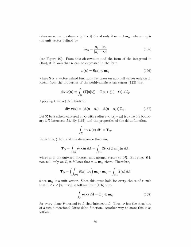
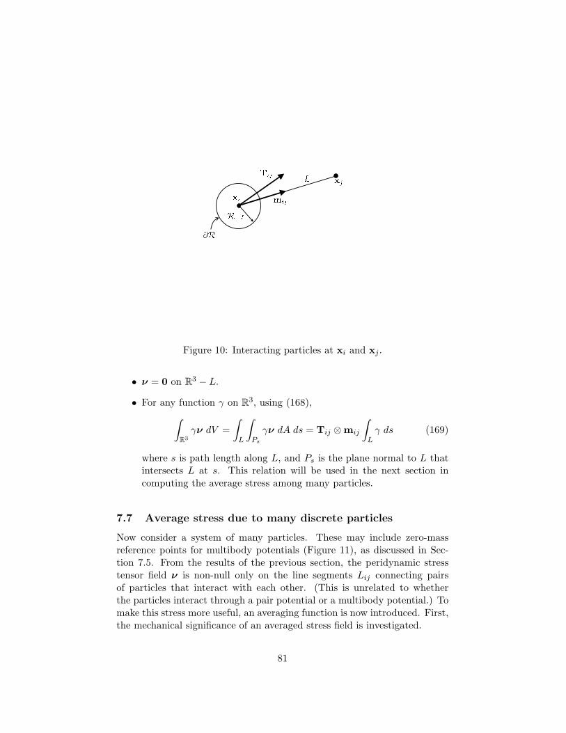
Section 7 demonstrates that a description of discrete particles can be ob-tained as the limiting case of peridynamic regions of finite volume as theirsizes are shrunk to zero. The resulting description involves forces that aremore general than pair interactions. Then, it is shown that such a collection
11
of “peridynamic particles” can be represented within the peridynamic con-tinuum equations using generalized functions. In particular, any multibodypotential can be represented exactly in terms of a peridynamic constitutivemodel. The peridynamic stress tensor and its volume average are derivedfor a system of discrete particles, and it is shown that these averages obeythe peridynamic equation of motion.
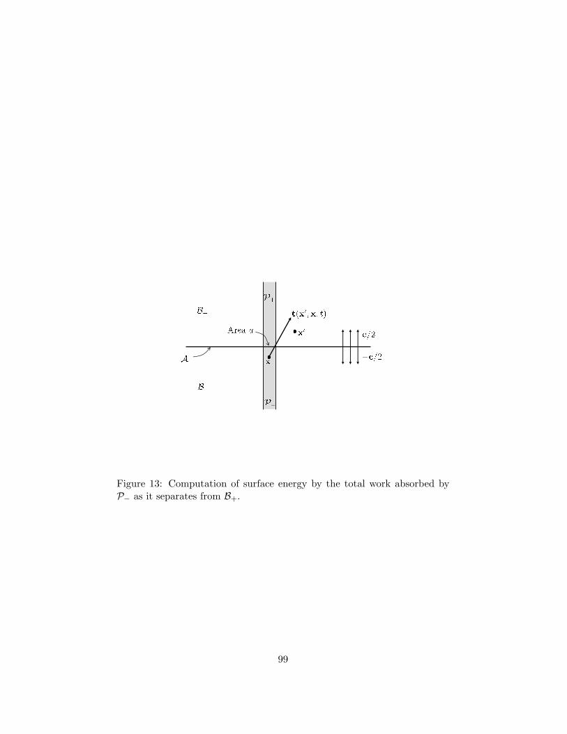
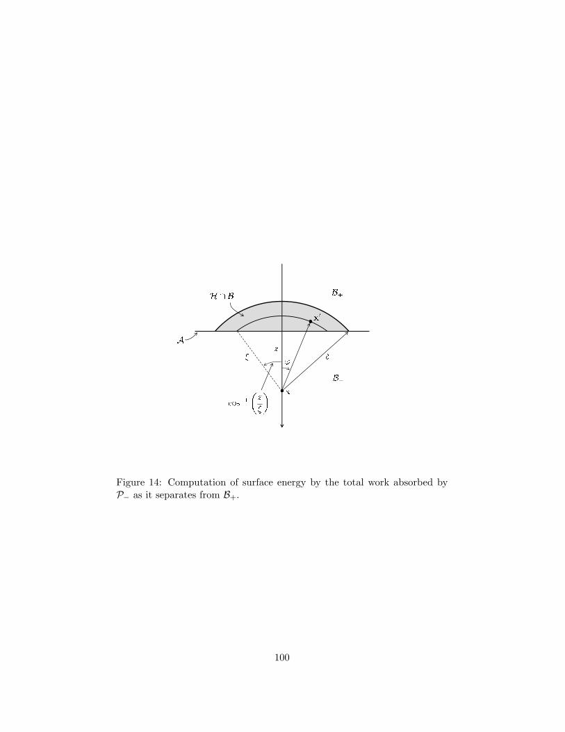
Damage and fracture are discussed in Section 8. It is shown how ir-reversible damage can be included in the peridynamic expression for freeenergy in a constitutive model. Damage evolution is treated as part of thematerial model. A peridynamic version of the J-integral is derived thatgives the rate of energy dissipation of a moving defect; this is related to theGriffith criterion for crack growth. An expression for the surface energy of acrack is derived in terms of the work done on bonds that initially connectedmaterial on one side of a crack to material on the other side.
12
2 Balance laws
We derive the peridynamic balances of linear and angular momentum in amore systematic way than has previously appeared in the literature [67].We then postulate the global balance of energy for a subregion in a peridy-namic body, which leads to the local balance of energy. The energy balanceinvolves both heat transport and mechanical power. The global energy bal-ance introduces the absorbed power and supplied power for a subregion. Animportant result is that the internal energy defined in terms of these powersis an additive quantity, leading to a meaningful definition of internal energydensity.
The balances of linear momentum, angular momentum, and energy areshown to adhere to a canonical structure, which we call the master balancelaw. This law expresses the rate of change of any additive quantity withina subregion as the sum of interactions between points inside and outsideof the subregion, plus a source term. These interactions appear withinthe integrand of an integral operator in the master balance law, and theantisymmetry of this integrand plays a crucial role. This antisymmetryallows the integral operator to be written as the integral of the divergenceof a nonlocal flux. (An analogous master balance law also exists in theclassical theory.)
2.1 Balance of linear momentum
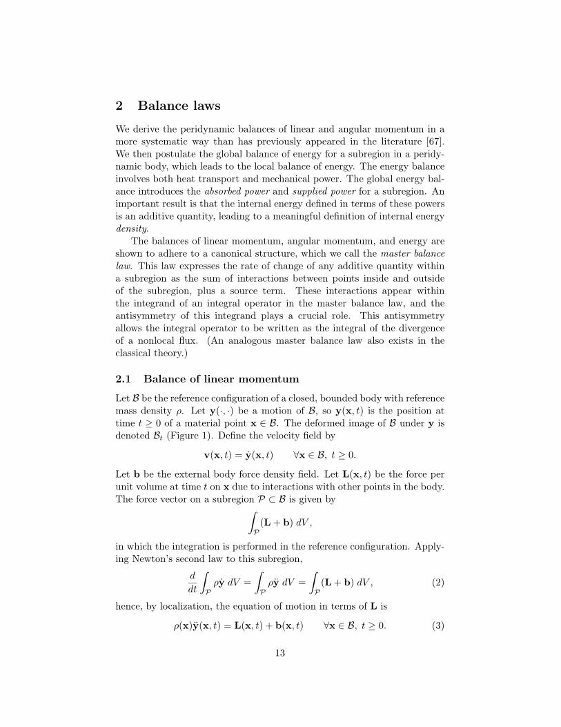
Let B be the reference configuration of a closed, bounded body with referencemass density ρ. Let y(·, ·) be a motion of B, so y(x, t) is the position attime t ≥ 0 of a material point x ∈ B. The deformed image of B under y isdenoted Bt (Figure 1). Define the velocity field by
v(x, t) = y(x, t) ∀x ∈ B, t ≥ 0.
Let b be the external body force density field. Let L(x, t) be the force perunit volume at time t on x due to interactions with other points in the body.The force vector on a subregion P ⊂ B is given by∫
P(L + b) dV ,
in which the integration is performed in the reference configuration. Apply-ing Newton’s second law to this subregion,
d
dt
∫Pρy dV =
∫Pρy dV =
∫P
(L + b) dV , (2)
hence, by localization, the equation of motion in terms of L is
Setting P = B in (2) and comparing the result with (4) shows that L mustbe self-equilibrated: ∫
BL(x, t) dVx = 0 ∀t ≥ 0.
Now let f(·, ·, ·) be a vector-valued function such that
L(x, t) =∫Bf(x′,x, t) dVx′ ∀x ∈ B, t ≥ 0, (5)
and such that f is antisymmetric:
f(x,x′, t) = −f(x′,x, t) ∀x,x′ ∈ B, t ≥ 0. (6)
For a given L, such an f can always be found; an example is
f(x′,x, t) =1V
(L(x, t)− L(x′, t)) (7)
where V is the volume of B in the reference configuration. The functionf , which plays a fundamental role in the peridynamic theory, is called thedual force density. It has dimensions of force per unit volume squared. Ingeneral, the vectors f(x′,x, t) and f(x,x′, t) are not parallel to the vectory(x′, t)−y(x, t). The particular choice of f given in (7) is not very useful inpractice; it is given only to demonstrate that for a given L, an f satisfying (5)and (6) always exists. In applications, f is determined by the deformationthrough the constitutive model.
The antisymmetry of f stated in (6) allows the balance of linear momen-tum on a subregion P ⊂ B to be expressed in a form in which f connectsonly points in the interior of P to points in its exterior. To see this, notethat (6) implies ∫
P
∫P
f(x′,x, t) dVx′ dVx = 0. (8)
Therefore, from (2), (5), and (8),
d
dt
∫Pρy(x, t) dV =
∫P
∫B\P
f(x′,x, t) dVx′ dVx +∫P
b(x, t) dVx. (9)
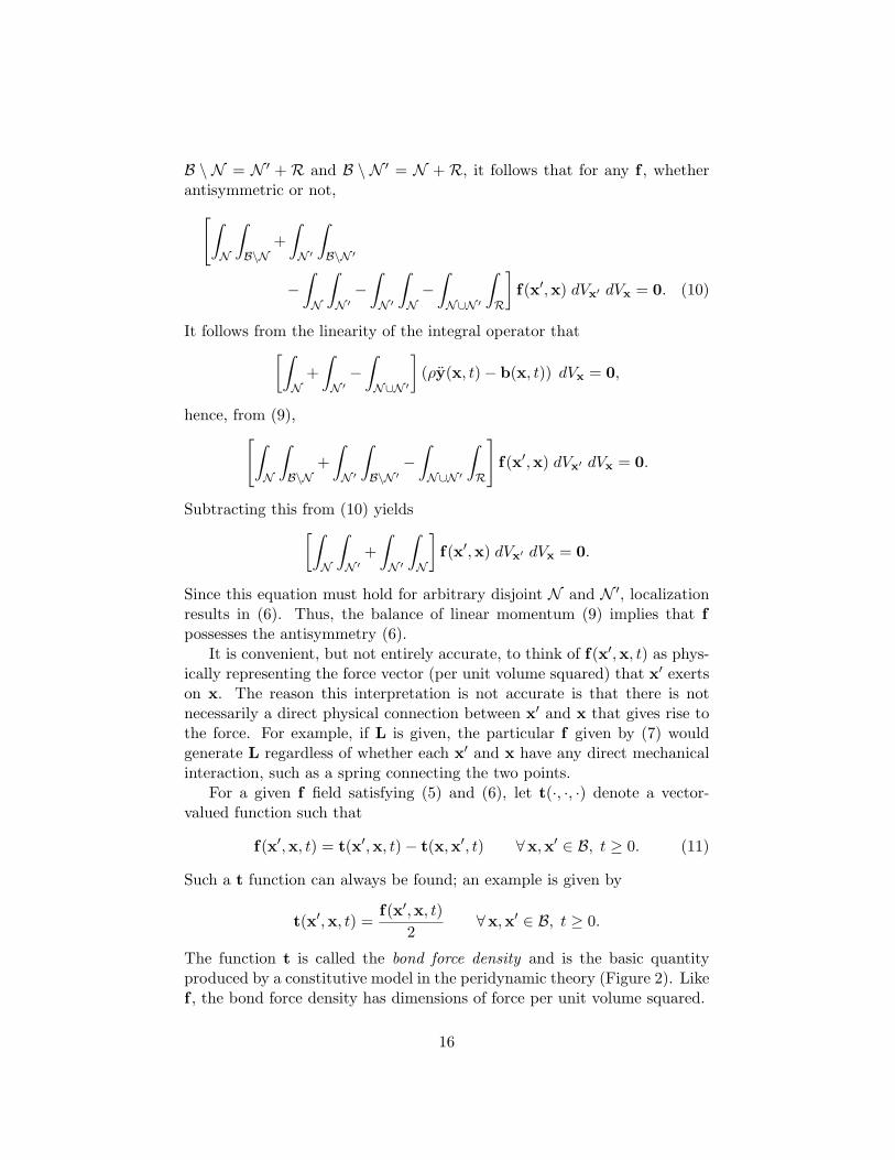
The following converse is also true: if (9) holds for all subregions P ⊂ B,then (6) holds. To see this, choose any two subregions N ⊂ B and N ′ ⊂ Bsuch that N ∩ N ′ = ∅ (Figure 3). Also define R = B \ (N ∪ N ′). Since
14
Figure 1: Peridynamic body and its motion y.
Figure 2: Dual force density f between two points has contributions fromthe bond force density t at both points.
15
B \ N = N ′ + R and B \ N ′ = N + R, it follows that for any f , whetherantisymmetric or not,[∫
N
∫B\N
+∫N ′
∫B\N ′
−∫N
∫N ′−∫N ′
∫N−∫N∪N ′
∫R
]f(x′,x) dVx′ dVx = 0. (10)
It follows from the linearity of the integral operator that[∫N
+∫N ′−∫N∪N ′
](ρy(x, t)− b(x, t)) dVx = 0,
hence, from (9),[∫N
∫B\N
+∫N ′
∫B\N ′
−∫N∪N ′
∫R
]f(x′,x) dVx′ dVx = 0.
Subtracting this from (10) yields[∫N
∫N ′
+∫N ′
∫N
]f(x′,x) dVx′ dVx = 0.
Since this equation must hold for arbitrary disjoint N and N ′, localizationresults in (6). Thus, the balance of linear momentum (9) implies that fpossesses the antisymmetry (6).
It is convenient, but not entirely accurate, to think of f(x′,x, t) as phys-ically representing the force vector (per unit volume squared) that x′ exertson x. The reason this interpretation is not accurate is that there is notnecessarily a direct physical connection between x′ and x that gives rise tothe force. For example, if L is given, the particular f given by (7) wouldgenerate L regardless of whether each x′ and x have any direct mechanicalinteraction, such as a spring connecting the two points.
For a given f field satisfying (5) and (6), let t(·, ·, ·) denote a vector-valued function such that
Such a t function can always be found; an example is given by
t(x′,x, t) =f(x′,x, t)
2∀x,x′ ∈ B, t ≥ 0.
The function t is called the bond force density and is the basic quantityproduced by a constitutive model in the peridynamic theory (Figure 2). Likef , the bond force density has dimensions of force per unit volume squared.
16
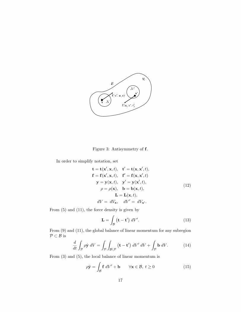
Figure 3: Antisymmetry of f .
In order to simplify notation, set
t = t(x′,x, t), t′ = t(x,x′, t),f = f(x′,x, t), f ′ = f(x,x′, t)
y = y(x, t), y′ = y(x′, t),ρ = ρ(x), b = b(x, t),
L = L(x, t),dV = dVx, dV ′ = dVx′ .
(12)
From (5) and (11), the force density is given by
L =∫B
(t− t′
)dV ′. (13)
From (9) and (11), the global balance of linear momentum for any subregionP ⊂ B is
d
dt
∫Pρy dV =
∫P
∫B\P
(t− t′
)dV ′ dV +
∫P
b dV . (14)
From (3) and (5), the local balance of linear momentum is
ρy =∫Bf dV ′ + b ∀x ∈ B, t ≥ 0 (15)
17
or equivalently, using (13),
ρy =∫B
(t− t′
)dV ′ + b ∀x ∈ B, t ≥ 0. (16)
The local balance of linear momentum is also called the equation of motion.By setting y = 0 in (16), the equilibrium equation is found to be∫
B
(t− t′
)dV ′ + b = 0 ∀x ∈ B.
The double integral in (14) represents a nonlocal flux of linear momentumthrough the boundary of P. This term is analogous to the contact force ona subregion in the classical, local theory. Equation (14) is an example ofnonlocal balance principles whose structure is discussed in Section 2.5.
2.2 Principle of virtual work
Boundary and initial conditions can be incorporated into the balance oflinear momentum (16) by formulating a variational problem [51]. Let B∗ ⊂B have a nonzero volume. B∗ consists of the points where the motion isprescribed. Let w(·, ·) be a motion of B, and use the abbreviated notation
w = w(x, t), w′ = w(x′, t).
The principle of virtual work is stated as follows:∫Bρy ·w dV +
∫B
∫Bt · (w′ −w) dV ′ dV =
∫Bb ·w dV (17)
for all motions w such that
w = 0 on B∗. (18)
We now demonstrate that the principle of virtual work implies the balanceof linear momentum. Using the change of variables x ↔ x′ leads to theidentity ∫
B
∫Bt · (w′ −w) dV ′ dV = −
∫B
∫B
(t− t′) ·w dV ′ dV . (19)
Inserting (19) into (17) results in∫B
(ρy −
∫B
(t− t′) dV ′ − b)·w dV = 0.
Since this must hold for any choice of w satisfying (18), it follows that
ρy =∫B
(t− t′) dV ′ + b on B \ B∗.
18
This leads to the initial boundary-value problem for the balance of linearmomentum (16)
ρy =∫B
(t− t′) dV ′ + b on B \ B∗,
y = y∗ on B∗,y(·, 0) = v0(·) on B \ B∗,
(20)
where y∗ and v0 are prescribed functions. Conversely, working backwardsshows that any solution of the initial boundary-value problem (20) alsosatisfies the principle of virtual work (PVW) statement (17).
2.3 Balance of angular momentum
Let B be a closed, bounded body, and as before, let P ⊂ B be a subregion.The angular momentum in P with respect to an arbitrary reference pointy0 is defined by
A(P) =∫P
(y − y0)× ρy dV . (21)
This definition asserts that there are no hidden variables or degrees of free-dom other than velocity that contain angular momentum. Since y×ρy = 0,(21) implies
A(P) =∫P
(y − y0)× ρy dV .
From this and (3),
A(P) =∫P
(y − y0)× (L + b) dV . (22)
Global balance of angular momentum on B requires that the rate of changeof total angular momentum equal the total moment due to external forces:
A(B) =∫B
(y − y0)× b dV . (23)
This equation asserts that there are no external moments other than thosearising from b. Comparing the last two equations and setting P = B placesa restriction on L: ∫
B(y − y0)× L dV = 0, (24)
which means that the moments generated by internal forces must be self-equilibrated. Conversely, (22) and (24) imply (23).
Suppose the bond force density field t is such that∫B
(y′ − y)× t dV ′ = 0 ∀x ∈ B, t ≥ 0. (25)
19
A bond force density field satisfying (25) will be called nonpolar. This nameis chosen to contrast the present situation with “micropolar” continuumtheories that permit a nonzero moment to be exerted on material points:the definition (25) asserts that the net moment about y(x, t) exerted byt(·,x) vanishes. Micropolar theory has been proposed, for example, as away of modeling granular flow [41]. A micropolar peridynamic model hasbeen proposed [30] but is beyond the scope of the present article.
If t is nonpolar, then the global balance of angular momentum on Bnecessarily holds. To see this, compute the left hand side of (24) using (5),(8), and (11):∫
B(y − y0)× L dV =
∫B
∫B
(y − y0)× f dV ′ dV
=∫B
∫By × f dV ′ dV − y0 ×
∫B
∫Bf dV ′ dV
=∫B
∫By × (t− t′) dV ′ dV .
Using the change of variables x↔ x′ to eliminate the t′ term and using (25)leads to ∫
B(y − y0)× L dV =
∫B
∫B
(y − y′)× t dV ′ dV = 0,
so (24) holds. As discussed above, this implies that the global balance ofangular momentum on B (23) holds.
Next, we further investigate the balance of angular momentum on subre-gions and use the results to derive the local balance of angular momentum.Assume that t is nonpolar, let P ⊂ B be a subregion, and let y0 = 0. From(5), (11) and (22),
A(P) =∫P
∫By × (t− t′) dV ′ dV +
∫P
y × b dV .
Add the expressiony′ × t− y′ × t
to the integrand in the double integral. Rearranging yields
A(P) =∫P
∫B
(y − y′)× t dV ′ dV
+∫P
∫B
(y′ × t− y × t′) dV ′ dV +∫P
y × b dV . (26)
20
Since the bond force densities are nonpolar, by (25), the first term on theright hand side vanishes. Also, the integrand in the second term is antisym-metric in x and x′, therefore∫
P
∫P
(y′ × t− y × t′) dV ′ dV = 0.
So, (26) implies
A(P) =∫P
∫B\P
(y′ × t− y × t′) dV ′ dV +∫P
y × b dV ,
or, recalling (21),
d
dt
∫P
y × ρy dV =∫P
∫B\P
(y′ × t− y × t′) dV ′ dV +∫P
y × b dV , (27)
which holds for any P ⊂ B. (22) and (27) are equivalent statements of theglobal balance of angular momentum for a subregion under the assumptionof nonpolar bond force densities. The structure of (27) is similar to thatof (14) in that the two terms on the right hand side represent nonlocal fluxand source rate. The underlying structure of balance principles of this typeis discussed further in Section 2.5.
By localizing (27), a form of the local balance of angular momentum isobtained:
y × ρy =∫B
(y′ × t− y × t′) dV ′ + y × b ∀x ∈ B, t ≥ 0.
This equation is equivalent to (25).
2.4 Balance of energy
Let q(x′,x, t) denote the rate of heat transport, per unit volume squared,from x′ to x. It is required that q be antisymmetric:
q(x,x′, t) = −q(x′,x, t) ∀x,x′ ∈ B, t ≥ 0. (28)
Nonlocal heat transport is assumed here for consistency with the mechanicalmodel, although the subsequent development of the energy balance couldbe repeated with a local heat model. Nonlocality is important in radiativeheat transport. In the limit of small interaction distances, nonlocal heatconduction is physically the same as the local model.
Let r(x, t) denote the heat source rate at x. The rate at which heat issupplied to a subregion P ⊂ B is given by
Q(P) =∫P
∫B\P
q dV ′ dV +∫Pr dV , (29)
21
where the abbreviation q = q(x′,x, t) is used. Taking the scalar product ofboth sides of the balance of linear momentum (16) with the velocity v andintegrating over P results in
d
dt
∫P
ρv · v2
dV =∫P
∫B
(t− t′
)· v dV ′ dV +
∫P
b · v dV . (30)
The identity (t− t′
)· v =
(t · v′ − t′ · v
)− t ·
(v′ − v
)implies that for all P ⊂ B,∫
P
∫B
(t− t′
)· v dV ′ dV
=∫P
∫B
(t · v′ − t′ · v
)dV ′ dV −
∫P
∫Bt ·(v′ − v
)dV ′ dV ,
=∫P
∫B\P
(t · v′ − t′ · v
)dV ′ dV −
∫P
∫Bt ·(v′ − v
)dV ′ dV ,
(31)
where the antisymmetry of the dual power density defined by
pd(x′,x) = t · v′ − t′ · v (32)
was used in the last step. Using (31), we may rewrite (30) as the powerbalance
K(P) +Wabs(P) =Wsup(P) (33)
where the kinetic energy in P is defined by
K(P) =∫P
ρv · v2
dV ,
the power absorbed by P is defined by
Wabs(P) =∫P
∫Bt ·(v′ − v
)dV ′ dV , (34)
and the power supplied to P is defined by
Wsup(P) =∫P
∫B\P
(t · v′ − t′ · v
)dV ′ dV +
∫P
b · v dV .
We postulate the following global form of the first law of thermodynamics:
E(P) + K(P) =Wsup(P) +Q(P) (35)
22
where E(P) is the internal energy in P. Subtracting (33) from (35) resultsin
E(P) =Wabs(P) +Q(P). (36)
This result asserts that the rate of change of internal energy is the sum ofthe absorbed power and the rate of heat supplied.
Using (28), it follows from the definitions (29) and (34) that both Wabs
and Q are additive quantities, i.e., for P1,P2 ⊂ B where P1 ∩ P2 = ∅,
Therefore, by (36), the internal energy E is also additive. It follows thatthere exists a scalar quantity ε(x, t) called the internal energy density suchthat
E(P) =∫Pε dV . (39)
From (29), (34), (36), and (39),∫Pε dV =
∫P
∫Bt ·(v′ − v
)dV ′ dV +
∫P
∫B\P
q dV ′ dV +∫Pr dV . (40)
By (28), ∫P
∫B\P
q dV ′ dV =∫P
∫Bq dV ′ dV .
From this and (40),∫P
[−ε+
∫Bt ·(v′ − v
)dV ′ +
∫Bq dV ′ + r
]dV = 0.
Since this must hold for any P ⊂ B, localization leads to the local statementof the first law of thermodynamics:
ε = pabs + h+ r. (41)
where the local heat transport rate at x is defined by
h =∫Bq dV ′
and the absorbed power density at x is defined by
pabs =∫Bt ·(v′ − v
)dV ′. (42)
pabs is the analogue of the stress power in the classical theory.
23
It is worthwhile to contrast the peridynamic power balance developedin this section with earlier approaches that lead to nonadditive definitionsof internal energy. The key difference lies in our usage of the peridynamicquantities absorbed and supplied power, rather than the traditional ideas ofinternal and external power that appear in literature on the thermodynamicsof nonlocal media. To see this, define the internal and external power by
Wint(P) =∫P
∫P
f · v dV ′ dV ,
Wext(P) =∫P
∫B\P
f · v dV ′ dV +∫P
b · v dV .
Wint(P) consists of the rate of work done on material points in P by inter-actions with other points in P. Wext(P) represents the work done by allother interactions, including body forces. These quantities are related toWabs and Wsup via
Wabs(P) = −Wint(P) +∫P
∫B\P
t ·(v′ − v
)dV ′ dV
Wsup(P) =Wext(P) +∫P
∫B\P
t ·(v′ − v
)dV ′ dV .
Inserting the above expressions for the absorbed and supplied power replaces(33) with the following alternate statement of the power balance:
K(P)−Wint(P) =Wext(P).
However, Gurtin and Williams [36] demonstrate thatWint andWext are notadditive quantities, in the sense of (38), leading to their conclusion that thereis no additive notion of the internal energy density analogous to (36). Theantisymmetretry of the dual power density pd defined in (32) is also necessaryfor the additivity of the absorbed and supplied power expenditures. As thenext section demonstrates, additivity and antisymmetry are intrinsic to wellformulated nonlocal balance laws.
2.5 Master balance law
The global balances of linear momentum (14), angular momentum (27),and energy (35) over any subregion P ⊂ B possess the following canonicalstructure:
E(P) =∫P
∫B\P
D dV ′ dV +∫P
s dV , (43)
where D(·, ·) : B × B → Rd and s(·) : B → Rd. Here, d = 1 if E is scalarvalued or d = 3 if it is vector valued. It is assumed that D is antisymmetric:
D(x′,x) = −D(x,x′) ∀x,x′ ∈ B. (44)
24
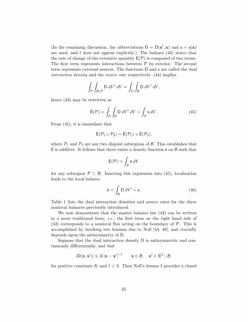
(In the remaining discussion, the abbreviations D = D(x′,x) and s = s(x)are used, and t does not appear explicitly.) The balance (43) states thatthe rate of change of the extensive quantity E(P) is composed of two terms.The first term represents interactions between P its exterior. The secondterm represents external sources. The functions D and s are called the dualinteraction density and the source rate respectively. (44) implies∫
P
∫B\P
D dV ′ dV =∫P
∫B
D dV ′ dV ,
hence (43) may be rewritten as
E(P) =∫P
∫B
D dV ′ dV +∫P
s dV . (45)
From (45), it is immediate that
E(P1 ∪ P2) = E(P1) + E(P2),
where P1 and P2 are any two disjoint subregions of B. This establishes thatE is additive. It follows that there exists a density function e on B such that
E(P) =∫P
e dV
for any subregion P ⊂ B. Inserting this expression into (45), localizationleads to the local balance
e =∫B
D dV ′ + s. (46)
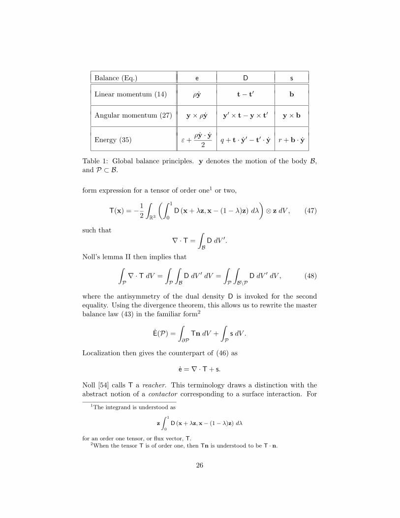
Table 1 lists the dual interaction densities and source rates for the threenonlocal balances previously introduced.
We now demonstrate that the master balance law (43) can be writtenin a more traditional form, i.e., the first term on the right hand side of(43) corresponds to a nonlocal flux acting on the boundary of P. This isaccomplished by invoking two lemmas due to Noll [53, 49], and cruciallydepends upon the antisymmetry of D.
Suppose that the dual interaction density D is antisymmetric and con-tinuously differentiable, and that
|D(x,x′)| 6 K|x− x′|−` x ∈ B, x′ ∈ R3 \ B,
for positive constants K and ` < 3. Then Noll’s lemma I provides a closed
25
Balance (Eq.) e D s
Linear momentum (14) ρy t− t′ b
Angular momentum (27) y × ρy y′ × t− y × t′ y × b
Energy (35) ε+ρy · y
2q + t · y′ − t′ · y r + b · y
Table 1: Global balance principles. y denotes the motion of the body B,and P ⊂ B.
form expression for a tensor of order one1 or two,
T(x) = −12
∫R3
(∫ 1
0D (x + λz,x− (1− λ)z) dλ
)⊗ z dV , (47)
such that∇ · T =
∫B
D dV ′.
Noll’s lemma II then implies that∫P∇ · T dV =
∫P
∫B
D dV ′ dV =∫P
∫B\P
D dV ′ dV , (48)
where the antisymmetry of the dual density D is invoked for the secondequality. Using the divergence theorem, this allows us to rewrite the masterbalance law (43) in the familiar form2
E(P) =∫∂P
Tn dV +∫P
s dV .
Localization then gives the counterpart of (46) as
e = ∇ · T + s.
Noll [54] calls T a reacher. This terminology draws a distinction with theabstract notion of a contactor corresponding to a surface interaction. For
1The integrand is understood as
z
∫ 1
0
D (x + λz,x− (1 − λ)z) dλ
for an order one tensor, or flux vector, T.2When the tensor T is of order one, then Tn is understood to be T · n.
26
instance, when the interaction is a force, a contactor is a contact stressassociated with the classical continuum notion of contact force.
The conclusion of Noll’s lemma II given by (48) implies that∫∂B
Tn dV = 0,
and equivalently expresses that the sum of the internal interactions in thebody is zero.
As shown in Section 2.1 for the case D = f , the second equality in(48) implies the antisymmetry of D that was assumed in (44). Lehoucqand Silling [48] provide an expression (see (120) below) for the peridynamicstress tensor in terms of the bond force density. This expression is derivablefrom (47) with D = f .
27
Figure 4: The family H contains the relative position vectors (bonds) con-necting x to points such as x′ within a distance δ of x.
3 Peridynamic states: notation and properties
The remainder of this paper largely involves mappings from pairs of points(x,x′) to some quantity. As an aid to keeping track of these mappings, itis convenient to introduce objects called “peridynamic states.” Consider abody B. Let δ be a positive number, called the horizon. For a given x ∈ B,let Hx be the neighborhood of radius δ with center x (Figure 4). Define thefamily of x by
H =ξ ∈ (R3 \ 0)
∣∣ (ξ + x) ∈ (Hx ∩ B).
A vector ξ ∈ H is called a bond connected to x. H differs from Hx in thatthe former is centered at 0 and contains bonds, while the latter is centeredat x and contains position vectors of material points.
A peridynamic state A〈 · 〉 is a function on H. The angle brackets 〈 · 〉enclose the bond vector; parentheses and square brackets will be used laterto indicated dependencies of the state on other quantities. A state need notbe a differentiable or continuous function of the bonds in H.
If the value A〈ξ〉 is a scalar, then A is a scalar state. The set of all scalarstates is denoted S. Two special scalar states are the zero state and the
28
unity state defined respectively by
0〈ξ〉 = 0, 1〈ξ〉 = 1 ∀ξ ∈ H.
If the value of A〈ξ〉 is a vector, then A is a vector state. The set of all vectorstates is denoted V. Two special vector states are the null vector state andthe identity state defined by
0〈ξ〉 = 0, X〈ξ〉 = ξ ∀ξ ∈ H (49)
where 0 is the null vector.An example of a scalar state is given by
a〈ξ〉 = 3c · ξ ∀ξ ∈ H,
where c is a constant vector. An example of a vector state is given by
A〈ξ〉 = ξ + c ∀ξ ∈ H.
Another useful kind of state, called a double state, maps pairs of bondsξ, ζ ∈ H into second order tensors, and is written A〈ξ, ζ〉. The set of alldouble states is denoted D.
In the following, a and b are scalar states, A and B are vector states, andV is a vector. Some elementary operations on states are defined as follows,for any ξ ∈ H:
(a+ b)〈ξ〉 = a〈ξ〉+ b〈ξ〉, (A + B)〈ξ〉 = A〈ξ〉+ B〈ξ〉
(ab)〈ξ〉 = a〈ξ〉b〈ξ〉, (aB)〈ξ〉 = a〈ξ〉B〈ξ〉
(A ·B)〈ξ〉 = A〈ξ〉 ·B〈ξ〉, (A⊗B)〈ξ〉 = (A〈ξ〉)⊗ (B〈ξ〉)
(A B)〈ξ〉 = A⟨B〈ξ〉
⟩, (A ·V)〈ξ〉 = (A〈ξ〉) ·V
where the symbol · indicates the usual scalar product of two vectors in R3
and ⊗ denotes the dyadic (tensor) product of two vectors. Also define ascalar state |A| by
|A|〈ξ〉 = |A〈ξ〉| (50)
and the dot products
a • b =∫Ha〈ξ〉b〈ξ〉 dVξ, A •B =
∫H
A〈ξ〉 ·B〈ξ〉 dVξ (51)
where, once again, the symbol · denotes the scalar product of two vectors inR3. The norm of a scalar state or a vector state is defined by
||a|| = √a • a, ||A|| =√
A •A. (52)
29
Most of the constitutive models in peridynamics involve functions of states,and it is helpful to define a notion of derivatives of such functions. If ψ(·) :S → R is a function of a scalar state, its Frechet derivative ∇ψ, if it exists,is defined by
ψ(A+ a) = ψ(A) +∇ψ(A) • a+ o(||a||) (53)
for all scalar states A and a. ∇ψ is a scalar state.If Ψ(·) : V → R is a function of a vector state, its Frechet derivative ∇Ψ,
if it exists, is similarly defined by
Ψ(A + a) = Ψ(A) +∇Ψ(A) • a + o(||a||) (54)
for all vector states A and a. ∇Ψ is a vector state.For functions of more than one state, for example Ψ(A,B), the Frechet
derivatives with respect to the two arguments will be denoted ΨA and ΨB
respectively. The notation ∂/∂A denotes the derivative of a function withrespect to A, if the argument depends either directly or indirectly on A.For example, if f(·) : R→ R, then
∂
∂Af(ψ(A)) = ∇φ(A), φ(A) := f(ψ(A)).
In this case, it is easily shown from (53) that the following chain rule applies:
∂
∂Af(ψ(A)) = f ′(ψ(A))∇ψ(A).
where f ′ denotes the first derivative of f .The operations on states such as the dot product defined above occur
repeatedly in manipulations, but their use does not restrict the physics thatcan be modeled. Note that S, V, and D are infinite dimensional linearvector spaces (assuming that H contains an infinite number of bonds), butthis does not preclude the modeling of nonlinear behavior. For example, thediscussion of constitutive modeling in Section 4 below deals with nonlinearfunctions of states.
A state field is a state valued function of position in B and possibly time.These dependencies are written in square brackets:
A[x, t]
for any x ∈ H and t ≥ 0. An example of a scalar state field is given by
a[x, t]〈ξ〉 = |ξ + x|t ∀ξ ∈ H, x ∈ B, t ≥ 0.
Finally, the dependence of a state valued function of other quantities iswritten in parentheses, for example
A(B).
30
An example of a state valued function of a vector state is given by
a(B) = |B|3,
i.e., using the definition (50),
a(B)〈ξ〉 = |B〈ξ〉|3 ∀ξ ∈ H, x ∈ B, t ≥ 0.
A vector state is analogous to a second order tensor in the classicaltheory, because it maps vectors (bonds) into vectors. However, the mappingperformed by a vector state is not necessarily a linear transformation onthe bond vectors, i.e., A〈ξ〉 is not necessarily a linear function of ξ. Theadditional notation described above is needed because of this nonlinearityand nonlocality.
The mappings defined by states provide the fundamental objects onwhich constitutive models operate in the nonlocal setting of peridynamics.In the classical theory, a constitutive model for a simple material specifiesa tensor (stress) as a function of another tensor (deformation gradient).In the peridynamic theory, a constitutive model instead provides a vectorstate (called the force state) as a function of another vector state (called thedeformation state). The way this works is discussed in the next section.
31
4 Constitutive modeling
The discussion in Section 2 introduced the bond force density field t withoutspecifying how this t is determined in a particular motion. This determi-nation is provided by the constitutive model, also called the material model,which contains all information about the response of a particular mate-rial. In the peridynamic theory, the constitutive model supplies t(x′,x, t) interms of the deformation at any given time, the history of deformation, andany other physically relevant quantities. This discussion does not includedamage, which is the subject of Section 8.
The state that maps bonds connected to x into their deformed images iscalled the deformation state and denoted Y[x, t]. Angle brackets are usedto indicate a bond that this state operates on. For a motion y, at any t ≥ 0,
Y[x, t]〈x′ − x〉 = y(x′, t)− y(x, t) (55)
for any x ∈ B and any x′ ∈ B such that x′ − x ∈ H (Figure 5). The valuesof any t(x′,x, t) are given by the force state T:
t(x′,x, t) = T[x, t]〈x′ − x〉. (56)
With this definition, the absorbed power density defined in (42) takes theform
pabs = T • Y (57)
where the dot product is defined in the previous section. Recall that thisabsorbed power density is the peridynamic analogue of the stress powerσ · F, where σ is the Piola stress tensor and F = ∂y/∂x is the deformationgradient tensor.
In terms of the force state, the equation of motion (16) has the form
ρ(x)y(x, t) =∫B
(T[x, t]〈x′ − x〉 −T[x′, t]〈x− x′〉
)dVx′ + b(x, t) (58)
for all x ∈ B, t ≥ 0. The equilibrium equation is then∫B
(T[x]〈x′ − x〉 −T[x′]〈x− x′〉
)dVx′ + b(x) = 0
for all x ∈ B.
4.1 Simple materials
The constitutive model determines the force state at any x and t. For asimple material and a homogeneous body, the force state depends only onthe deformation state:
T[x, t] = T(Y[x, t])
32
Figure 5: The deformation state Y[x, t] maps each bond in the family of xto its deformed image.
33
where T(·) : V → V is a function whose value is a force state. Suppressingfrom the notation the dependence on x and t,
T = T(Y) (59)
which is analogous to the Piola stress in a simple material in the classicaltheory, σ = σ(F). If the body is heterogeneous, an explicit dependence onx is included:
T = T(Y,x).
If the material is rate dependent, the constitutive model would additionallydepend on the time derivative of the deformation state:
T = T(Y, Y,x).
4.2 Kinematics of deformation states
The deformation state defined in (55) provides a mapping from each bondξ in the family of x to its deformed image Y〈ξ〉. It is assumed that at anyt ≥ 0, y(·, t) is invertible:
x1 6= x2 =⇒ y(x1, t) 6= y(x2, t) ∀x1,x2 ∈ B.
This assumption implies
Y〈ξ〉 6= 0 ∀ξ ∈ H.
Otherwise, there are essentially no kinematical restrictions on Y. All of thefollowing are allowed:
• Nondifferentiability (as might occur near an inclusion or a phase bound-ary).
• Discontinuities (such as a crack).
• Voids and other defects.
However, not all these allowable features would appear, or be capable ofappearing, in a given application.
4.3 Directional decomposition of a force state
As discussed in Section 2.3, bond force densities are assumed to be non-polar, as defined in (25). This provides an admissibility condition on theconstitutive model. In terms of the force state, the condition for nonpolarityis written as ∫
HY〈ξ〉 × T(Y)〈ξ〉 dVξ = 0 ∀Y ∈ V. (60)
34
This requirement means that the force state at x exerts no net moment ona small volume surrounding B \ x.
For any deformation state Y, define the direction state by
M =Y|Y|
(61)
(see (50) for notation). Using the abbreviation T = T(Y), define thecollinear and orthogonal parts of the force state by
T‖ = (M⊗M)T, T⊥ = T−T‖. (62)
Thus, for any ξ ∈ H,
T‖〈ξ〉 = (M〈ξ〉 ·T〈ξ〉)M〈ξ〉 (63)
which is parallel to the deformed bond. Similarly, T⊥〈ξ〉 is orthogonal tothe deformed bond. From (61) and (63),∫
HY〈ξ〉 ×T‖〈ξ〉 dVξ = 0
regardless of constitutive model. From this and the second of (62), thecondition for nonpolarity (60) is equivalent to∫
HY〈ξ〉 ×T⊥〈ξ〉 dVξ = 0.
The constitutive model T is called ordinary if, for all Y ∈ V,
T‖ = T (64)
where T = T(Y). Otherwise, the constitutive model is nonordinary. From(60) and (64), evidently all ordinary constitutive models are nonpolar. (Theconverse of this is not true.)
4.4 Examples
An example of a simple peridynamic material model is given by
T(Y) = a(|Y| − |X|
)M, M =
Y|Y|
∀Y ∈ V,
where a is a constant. Writing this out in detail,
T〈ξ〉 = a(|Y〈ξ〉| − |ξ|
) Y〈ξ〉|Y〈ξ〉|
∀Y ∈ V,
35
for any bond ξ ∈ H. In this material, the magnitude of the bond forcedensity vector t is proportional to the bond extension (change in length ofthe bond). The direction is parallel to the deformed bond. In this exam-ple, the bonds respond independently of each other: T〈ξ〉 depends only onY〈ξ〉. Materials with this property are called bond-based and are discussedin Section 4.7.
A much larger class of materials incorporates the collective response ofbonds. This means that the force density in each bond depends not only onits own deformation, but also on the deformation of other bonds. A simpleexample is given by
T〈ξ〉 = a(|Y〈ξ〉| − |Y〈 − ξ〉|
)M〈ξ〉.
In this material, the bond force density for any bond ξ is proportional tothe difference in deformed length between itself and the bond opposite toξ. (Note that in general Y〈 − ξ〉 6= −Y〈ξ〉, since the two bonds ξ and −ξcan deform independently of each other.) This material is an example of abond-pair model, discussed in Section 4.12.
The mean elongation of all the bonds in a family is defined by
e =1VH
∫H
(|Y〈ξ〉| − |ξ|
)dVξ, VH =
∫HdV.
A material model in which the magnitudes of forces in the bonds are identicalto each other and depend only on the mean elongation is provided by
T = aeM.
In Section 4.10, the mean elongation in the bonds (weighted by scalar state)is used to define a nonlocal volume change. This provides a way to char-acterize an isotropic solid using the conventional bulk modulus and shearmodulus.
4.5 Thermodynamic restrictions on constitutive models
In this section it is shown that the force state can be related to a free energyfunction, which is subject to certain restrictions due to the second law ofthermodynamics. The first law of thermodynamics asserts the equivalenceof mechanical energy and heat energy. At any point x ∈ B, the local formof the first law (41) with the absorbed power density given by (57) takes theform
ε = T • Y + h+ r (65)
where ε is the internal energy density, h is the rate of heat transfer dueto interaction with other points in B, and r is a prescribed source rate (allthese quantities are per unit volume in the reference configuration).
36
The second law of thermodynamics is expressed by the Clausius-Duheminequality:
θη ≥ r + h (66)
where θ is the absolute temperature and η is the entropy density. Now definethe free energy density by
ψ = ε− θη. (67)
Following Coleman and Noll [15], certain restrictions on the constitutiveresponse will now be derived. Taking the time derivative of (67) leads to
ψ = ε− θη − θη.
From this and (65), it follows that
ψ = T • Y + h+ r − θη − θη. (68)
Combining this expression with (66), the variables ε, η, and r are eliminatedto yield
T • Y − θη − ψ ≥ 0. (69)
Now assume that ψ and η have the following dependencies:
ψ = ψ(Y, Y, θ), η = η(Y, Y, θ),
hence ψ involves the Frechet derivatives of ψ with respect to Y and Y,which are denoted ψY and ψY respectively:
ψ = ψY • Y + ψY • Y + ψθθ,
with a similar expression for η. Combining these with (69) leads to(T− ψY
)• Y − ψY • Y −
(ψθ + η
)θ ≥ 0. (70)
The method of Coleman and Noll assumes that, in the present case of peri-dynamics, the quantities Y, Y, and θ can, in principle, be varied indepen-dently. The inequality (70) must hold for all such choices. This results inthe following conclusions:
η = −ψθ, ψY = 0.
The first of these is a standard relation in thermodynamics. The secondstates that the free energy is independent of Y. Next, following Fried’sdevelopment [29] for the thermodynamics of discrete particles, decomposethe force state into parts that are independent of and dependent on Yrespectively:
T(Y, Y, θ) = Te(Y, θ) + Td(Y, Y, θ) (71)
37
where the superscript e stands for “equilibrium” and d stands for “dissipa-tive.” Then, setting θ = 0 and Y = 0 in (70) and using (71),(
Te(Y, θ)− ψY(Y, θ))• Y + Td(Y, Y, θ) • Y ≥ 0
where the terms that are independent of Y have been grouped together.The conclusions are therefore
Te(Y, θ) = ψY(Y, θ) (72)
andTd(Y, Y, θ) • Y ≥ 0. (73)
Equation (73) is the dissipation inequality for rate-dependent materials inperidynamics, and it must hold for all choices of Y. It states that therate-dependent part of the constitutive model must dissipate energy at anonnegative rate. Interestingly, (73) does not imply that
Td〈ξ〉 · Y〈ξ〉 ≥ 0 ∀ξ ∈ H.
In other words, there can be some bonds that “generate energy” providedthere are other bonds that dissipate at least this much energy. A version ofthe dissipation inequality for materials undergoing damage will be discussedin Section 8.2.
4.6 Elastic materials
If the free energy density depends only on Y, the material is called elastic,and by convention the free energy density is called the strain energy densityand denoted W = W (Y). Then by (72),
W = T • Y (74)
for any Y andT = WY.
Since W is a function of only one variable, this can also be written as
T = ∇W . (75)
For a body composed of an elastic material (not necessarily homogeneous),by setting w = y in the principle of virtual work expression (17) and using(56) and (74), it follows that for an elastic material,
d
dt
∫B
ρy · y2
dV +d
dt
∫BW dV =
∫Bb · y dV .
38
Thus, as in the classical theory, work performed on an elastic peridynamicbody by external loads is converted into a combination of kinetic energy andrecoverable strain energy.
A mechanical interpretation of the Frechet derivative of W in an elasticmaterial is as follows. Suppose the family is deformed, then held fixed.Choose a single bond ξ, surrounded by a small volume dV . While continuingto hold all other bonds fixed, increment the position of the small volume by asmall vector ε. If the material is elastic, then there is a vector t, independentof ε, such that the resulting change in W is given by
dW = t · ε dV .
The value of this vector is t = T〈ξ〉. An elastic material model can be eitherordinary or nonordinary: elasticity does not require that T〈ξ〉 ‖ Y〈ξ〉.
4.7 Bond-based materials
Suppose that each bond has its own constitutive relation, independent ofthe others. Then there is a function t(·, ·) on R3 ×H such that
T〈ξ〉 = t(Y〈ξ〉, ξ) (76)
for all Y ∈ V and all ξ ∈ H. Such a material model is called bond-based.The requirement of nonpolarity (60) implies that any bond-based mate-
rial model is ordinary. To see this, suppose that it is nonordinary. Then, bydefinition, there is some deformation state Y0 and some bond ξ0 such that
c := Y0〈ξ0〉 × t0 6= 0, t0 = t(Y0〈ξ0〉, ξ0).
Start with this Y0 and let all other bonds except ξ0 be held fixed whileξ0 is further deformed. (Strictly speaking, we are deforming the materialpoint x + ξ0, while holding all other material points fixed, where x is thepoint whose constitutive model is under consideration.) Because (60) mustcontinue to hold during this process, any choice of Y〈ξ0〉 leaves Y〈ξ0〉 ×t(Y〈ξ0〉, ξ0) unchanged, i.e.,
z× t(z, ξ0) = c (77)
for any vector z = Y〈ξ0〉. One such choice is
z = αc
where α is a nonzero scalar with the appropriate dimensions for this expres-sion to make sense. Then by (77),
αc× t(αz, ξ0) = c.
39
This can only hold if c = 0, proving that the material model is ordinary.3
In an elastic bond-based body, there is a scalar-valued function w(p, ξ)called the bond potential, where p is a vector, such that
Note that the first argument of w in this integrand is a vector, not a vectorstate. wp denotes the partial derivative with respect to this argument.
Recall the result proved above that any bond-based material model isordinary. An implication of this result for elastic bond-based materials isthat w(p, ξ) can depend on p only through |p|, i.e., through the deformedlength of the bond. To confirm this, choose a deformed bond vector pand consider a rotation of this vector at some angular velocity ω. Thendp/dt = ω × p. Therefore
d
dtw(p, ξ) = wp(p, ξ) · dp
dt= wp(p, ξ) · (ω × p).
Since the material is ordinary, there is some scalar β, with appropriatedimensions, such that
wp(p, ξ) = βp.
Combining the last two equations,
d
dtw(p, ξ) = βp · (ω × p).
Since, for any vector ω, p ⊥ (ω × p), it follows that
d
dtw(p, ξ) = 0.
This proves that w(p, ξ) is unchanged by a rigid rotation of p; therefore, wdepends on p only through |p|. So, we can write, for an elastic bond-basedmaterial model,
w(p, ξ) = w(e, ξ), e = |p| − |ξ|
for some function w. Then, by the first of (78),
W (Y) =∫Hw(e〈ξ〉, ξ) dVξ,
3The discussion of this result in [60] is flawed because it treats only pairs of materialpoints in isolation from all other material points, neglecting the possibility that these otherpoints could somehow cancel out a couple between the pair.
40
where e is the scalar extension state, defined by
e = |Y| − |X| or e〈ξ〉 = |Y〈ξ〉| − |ξ| ∀ξ ∈ H.
Let the partial derivative of w(e, ξ) with respect to e be denoted we(e, ξ).By the second of (78) and the chain rule,
t(Y〈ξ〉, ξ) = we(e〈ξ〉, ξ)M, M =Y〈ξ〉|Y〈ξ〉|
. (79)
If the body is homogeneous and composed of bond-based material, it issometimes convenient to consider each bond as the fundamental object forpurposes of constitutive modeling: set
W (x) =12
∫Hx
w(e,x′,x
)dVx′ , e = |y(x′)− y(x)| − |x′ − x|
where Hx is the neighborhood of x with radius equal to the horizon, and
w(e,x′,x) = 2w(e,x′ − x).
This change allows the resulting “bond-based theory” to be developed with-out using the formalism of states. The bond-based theory is the subject of[60], in which w is called the micropotential and the material model is calledmicroelastic. Because the bond-based theory was developed earlier than thestate-based theory, and because its constitutive models do not require theadditional complexity of Frechet derivatives, the vast majority of applica-tions of peridynamics have been performed within the bond-based theory.However, as noted in Section 1.2, the bond-based theory suffers from severelimitations on the material response it can reproduce, notably the restric-tion on the Poisson ratio ν = 1/4 for isotropic microelastic solids. It isdemonstrated in Section 4.10 below that this restriction is removed in thestate-based theory.
4.8 Objectivity
As in the classical theory, invariance of a strain energy density function in theperidynamic theory with respect to rigid rotation following a deformationleads to a notion of material frame indifference, or objectivity. LetO+ denotethe set of all proper orthogonal tensors. For any Q ∈ O+ and any A ∈ V,let QA be the vector state defined by
(QA)〈ξ〉 = Q(A〈ξ〉) ∀ξ ∈ H
and similarly define the state AQ by
(AQ)〈ξ〉 = A〈Qξ〉 ∀ξ ∈ H.
41
Consider an elastic material such that
W (QY) = W (Y) ∀Q ∈ O+, Y ∈ V. (80)
Let Q be fixed. Consider any Y ∈ V and a small increment δY ∈ V. From(54), (75), and (80), neglecting terms of higher order than δY,
T(QY) • δ(QY) = T(Y) • δY.
Since T is vector valued, by the properties of the transpose of a tensor,(QT T(QY)
)• δY = T(Y) • δY.
Since this must hold for every small δY, and since QT = Q−1, it followsthat (80) implies
T(QY) = QT(Y) ∀Q ∈ O+, Y ∈ V. (81)
Any simple material model, whether elastic or not, that satisfies (81) iscalled objective. Objectivity can be assumed as an admissibility requirementfor any material model in the absence of some externally dictated specialdirection in space, such as an electric field. It is easily shown [63] that anobjective elastic material necessarily satisfies the condition for nonpolarity(60).
4.9 Isotropy
Consider an elastic material model with the property that
W (YQ) = W (Y) ∀Q ∈ O+, Y ∈ V. (82)
Proceeding as in the previous section, choose any Q ∈ O+ and any Y ∈ V,then consider a small increment δY ∈ V. From (54), (75), and (82),
T(Y) • δY = T(YQ) • δ(YQ)
=∫H
T(YQ)〈ξ〉 · δY〈Qξ〉 dVξ
=∫H
T(YQ)〈Q−1ξ′〉 · δY〈ξ′〉 dVξ′
=(T(YQ)Q−1
)• δY
where the change of variable ξ′ = Qξ has been used. Since this result musthold for every δY, it follows that (82) implies
T(YQ) = T(Y)Q ∀Q ∈ O+, Y ∈ V. (83)
Any material model, whether elastic or not, satisfying (83) is called isotropic.If the material model is isotropic, then the force state is invariant withrespect to pre-rotations applied before the stretch.
42
4.10 Isotropic elastic solid
A peridynamic material model for a constitutively linear isotropic elasticsolid was proposed in Section 15 of [67]. A nonlocal dilatation is defined by
ϑ =3m
(ωx) • e, m = (ωx) • x (84)
where ω is the scalar influence state, which serves as a weighting function,and the scalar extension state is defined by
e = |Y| − x, x = |X|.
It can be shown [67] that for any choice of ω, if the deformation is small andhomogeneous, ϑ defined in (84) equals the trace of the classical linear straintensor. (The coefficient 3/m in (84) is chosen so that this is true.)
Define an elastic material in which the strain energy density contains twoterms representing the contribution of the volume change and of everythingelse in the deformation state, respectively:
W (Y) =kϑ2
2+α
2(ωed) • ed (85)
where k and α are constants and
ed := e− ei, ei :=ϑx
3.
The scalar state ei is called the isotropic part of the extension state, and ed
is called the deviatoric part. The isotropic part contains length changes ofbonds due to isotropic expansion of the family. The deviatoric part containsthe remainder of the length changes, which may be due to shear or to othertypes of deformation within the family. After evaluating the applicableFrechet derivatives [67], the force state is given by
T(Y) =(
3kϑm
ωx+ αωed)
M, M =Y|Y|
.
Since the bond force densities are parallel to the deformed bonds, this is anordinary material model. This material model is constitutively linear in thesense that the force state depends linearly on the extension state. However,it does not assume linear kinematics as will be assumed in the linearizedperidynamic theory discussed below in Section 5. For small, homogeneousdeformations, the strain energy density in the peridynamic material model(85) equals that of an isotropic linear elastic solid in the classical theoryprovided k is the bulk modulus for the material and α = 15µ/m, where µ isthe shear modulus [67].
43
4.11 Peridynamic material derived from a classical material
Suppose a material model from the classical theory is given in the followingform:
σ = σ(F), F =∂y∂x
where σ is the Piola stress tensor, σ is a function, and F is the deformationgradient tensor. A peridynamic material model can be derived from this asfollows [67, 74, 27]. (An alternative approach making use of the principleof virtual work can also be used [51].) A nonlocal approximation to thedeformation gradient tensor is defined by
F =(∫Hω〈ξ〉Y〈ξ〉 ⊗ ξ dVξ
)K−1
where ω is the scalar influence state and K is the symmetric positive definiteshape tensor defined by
K =∫Hω〈ξ〉ξ ⊗ ξ dVξ.
The force state is determined by mapping the resulting σ back onto thebonds as follows:
T(Y) = ωσ(F)K−1X.
The peridynamic stress tensor (see Section 6.2) corresponding to this peri-dynamic material model equals σ(F) in the special case of homogeneousdeformation of a homogeneous body.
4.12 Bond-pair materials
Let w be a scalar-valued function of four vectors:
w(p,q, r, s)
with partial derivatives with respect to the first two arguments denoted by
wp(p,q, r, s), wq(p,q, r, s).
Suppose an elastic material has its strain energy density function given by
W (Y) =∫Hw(Y〈ξ〉,Y〈χ(ξ)〉, ξ,χ(ξ)) dVξ (86)
where χ(·) : H → H is a continuously differentiable and invertible function.(Note that the four arguments of w in the integrand are vectors, not vector
44
states, because Y is evaluated at the specific bonds ξ and χ(ξ).) Let χ−1
be the inverse mapping of χ:
ζ = χ(ξ) ⇐⇒ ξ = χ−1(ζ).
Let the Jacobian determinants of the forward and inverse mappings be de-fined by
J(ξ) =∣∣∣det grad χ(ξ)
∣∣∣, J−1(ζ) =∣∣∣det grad χ−1(ζ)
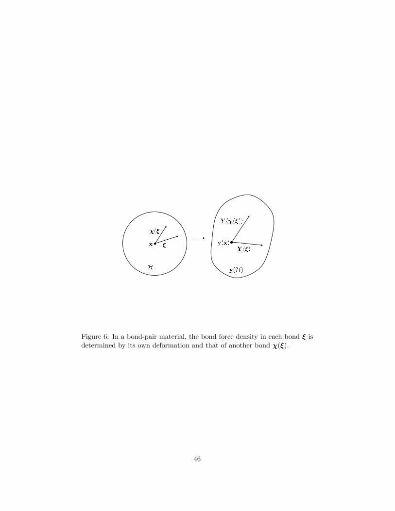
∣∣∣.Mechanically, the W defined in (86) sums up energies due to interactionsbetween pairs of bonds ξ and χ(ξ). Such a material is called a bond-pairmaterial (Figure 6).
To determine the associated force state, the Frechet derivative of this Wis evaluated as follows. Consider an increment in the deformation state δY.Then, from (86),
δW =∫H
[wp
(Y〈ξ〉,Y〈χ(ξ)〉, ξ,χ(ξ)
)· δY〈ξ〉
+ wq
(Y〈ξ〉,Y〈χ(ξ)〉, ξ,χ(ξ)
)· δY〈χ(ξ)〉
]dVξ.
Now use the change of variables ζ = χ(ξ) in the wq term to obtain
δW =∫Hwp
(Y〈ξ〉,Y〈χ(ξ)〉, ξ,χ(ξ)
)· δY〈ξ〉 dVξ
+∫Hwq
(Y〈χ−1(ζ)〉,Y〈ζ〉,χ−1(ζ), ζ
)· δY〈ζ〉 J−1(ζ) dVζ .
In the second integral, replace the dummy variable of integration ζ by ξ:
δW =∫H
[wp
(Y〈ξ〉,Y〈χ(ξ)〉, ξ,χ(ξ)
)+ wq
(Y〈χ−1(ξ)〉,Y〈ξ〉,χ−1(ξ), ξ
)J−1(ξ)
]· δY〈ξ〉 dVξ.
Comparing this result with (75), the force state can be read off:
T〈ξ〉 = ∇W 〈ξ〉 = wp
(Y〈ξ〉,Y〈χ(ξ)〉, ξ,χ(ξ)
)+ wq
(Y〈χ−1(ξ)〉,Y〈ξ〉,χ−1(ξ), ξ
)J−1(ξ). (87)
Bond-based materials are a special case of bond pair materials with χ〈ξ〉 = ξfor all ξ.
45
Figure 6: In a bond-pair material, the bond force density in each bond ξ isdetermined by its own deformation and that of another bond χ(ξ).
46
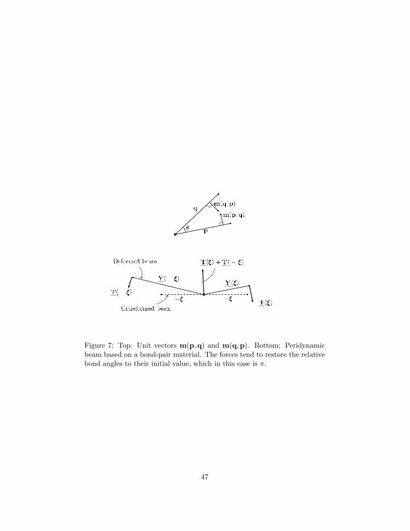
Figure 7: Top: Unit vectors m(p,q) and m(q,p). Bottom: Peridynamicbeam based on a bond-pair material. The forces tend to restore the relativebond angles to their initial value, which in this case is π.
47
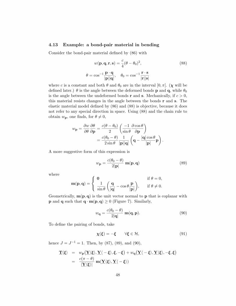
4.13 Example: a bond-pair material in bending
Consider the bond-pair material defined by (86) with
w(p,q, r, s) =c
4(θ − θ0)2, (88)
θ = cos−1 p · q|p||q|
, θ0 = cos−1 r · s|r||s|
where c is a constant and both θ and θ0 are in the interval [0, π]. (χ will bedefined later.) θ is the angle between the deformed bonds p and q, while θ0is the angle between the undeformed bonds r and s. Mechanically, if c > 0,this material resists changes in the angle between the bonds r and s. Theelastic material model defined by (86) and (88) is objective, because it doesnot refer to any special direction in space. Using (88) and the chain rule toobtain wp, one finds, for θ 6= 0,
wp =∂w
∂θ
∂θ
∂p=c(θ − θ0)
2
(−1
sin θ∂ cos θ∂p
)=c(θ0 − θ)
2 sin θ1|p||q|
(q− |q| cos θ
|p|p).
A more suggestive form of this expression is
wp =c(θ0 − θ)
2|p|m(p,q) (89)
where
m(p,q) =
0 if θ = 0,1
sin θ
(q|q|− cos θ
p|p|
), if θ 6= 0.
Geometrically, m(p,q) is the unit vector normal to p that is coplanar withp and q such that q ·m(p,q) ≥ 0 (Figure 7). Similarly,
wq =c(θ0 − θ)
2|q|m(q,p). (90)
To define the pairing of bonds, take
χ(ξ) = −ξ ∀ξ ∈ H, (91)
hence J = J−1 = 1. Then, by (87), (89), and (90),
T〈ξ〉 = wp
(Y〈ξ〉,Y〈 − ξ〉, ξ,−ξ
)+ wq
(Y〈 − ξ〉,Y〈ξ〉,−ξ, ξ
)=
c(π − θ)|Y〈ξ〉|
m(Y〈ξ〉,Y〈 − ξ〉)
48
whereθ = cos−1 Y〈ξ〉 ·Y〈 − ξ〉
|Y〈ξ〉||Y〈 − ξ〉|, 0 ≤ θ ≤ π.
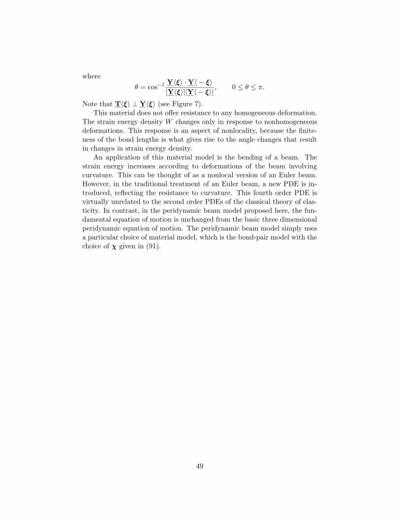
Note that T〈ξ〉 ⊥ Y〈ξ〉 (see Figure 7).This material does not offer resistance to any homogeneous deformation.
The strain energy density W changes only in response to nonhomogeneousdeformations. This response is an aspect of nonlocality, because the finite-ness of the bond lengths is what gives rise to the angle changes that resultin changes in strain energy density.
An application of this material model is the bending of a beam. Thestrain energy increases according to deformations of the beam involvingcurvature. This can be thought of as a nonlocal version of an Euler beam.However, in the traditional treatment of an Euler beam, a new PDE is in-troduced, reflecting the resistance to curvature. This fourth order PDE isvirtually unrelated to the second order PDEs of the classical theory of elas-ticity. In contrast, in the peridynamic beam model proposed here, the fun-damental equation of motion is unchanged from the basic three dimensionalperidynamic equation of motion. The peridynamic beam model simply usesa particular choice of material model, which is the bond-pair model with thechoice of χ given in (91).
49
5 Linear theory
Like the linear classical theory, the linear peridynamic theory concerns smalldeformations. However, the applicable notion of smallness is different in theperidynamic theory, because it does not restrict the deformation gradient,and even allows discontinuities. Under this assumption of smallness, theperidynamic equation of equilibrium reduces to a linear integral equation.
Linearization of the bond-based peridynamic theory is discussed in [60,83]. The discussion below pertains to the more general state-based theoryand largely follows [63]. See Section 1.2 for a summary of work to datemaking use of the linear theory.
5.1 Small displacements
Let B be a body with horizon δ. Consider a time-independent deformationy0, which may be large. (The role of y0 in the linearization will becomeclear in Section 5.3 below.) Let u be a displacement field superposed on y0,and define a vector state field by
(Strictly speaking, (93) is actually a condition on the relative displacements,rather than the displacements themselves.) This idea of a small displacementfield is a nonlocal analogue of the concept in classical linear theory that|grad u| 1. The peridynamic definition of a small displacement field (93)does not restrict rigid translations of a body, but it does restrict rigid bodyrotations to small angles. More importantly, it allows for possible smalldiscontinuities in u, a key difference from the classical linear theory.
Recalling the definition of the norm of a vector state (52), for a smalldisplacement field, (93) and (94) imply that
||U|| = O(`).
5.2 Double states
In the linear peridynamic theory, the analogue of the classical fourth orderelasticity tensor is a double state (see definition following (49)). Before de-veloping the linear theory further, it is helpful to introduce some propertiesof double states.
50
If D is a double state, then for every pair of bonds ξ and ζ inH, the valueof D〈ξ, ζ〉 is a second-order tensor. The set of all double states is denotedD. In the following, D and E are double states, while A and B are vectorstates. Define the vector state D •A by
(D •A)〈ξ〉 =∫H
D〈ξ, ζ〉 A〈ζ〉 dVζ ∀ξ ∈ H
where the integrand is the product of a second order tensor with a vector;the component form is DijAj . The adjoint of D is a double state defined by
D†〈ξ, ζ〉 = DT 〈ζ, ξ〉 ∀ξ, ζ ∈ H.
where the superscript T indicates the tensor transpose. Note that the orderof the bonds is switched when taking the adjoint in addition to taking thetensor transpose. D is self-adjoint if
D† = D.
Also define the vector state A • D by
A • D = D† •A.
For any vector states A and B, the following identity holds:
B • D† •A = A • D •B.
If S(·) : V → V is Frechet differentiable, then
S(A + a) = S(A) +∇S(A) • a + o(||a||) ∀A,a ∈ V (95)
where ∇S(A) is a double state. As before, in the case of a function oftwo states, such as S(A,B), the Frechet derivative with respect to each isdenoted SA or SB.
If Ψ(·) : V → R, then the second Frechet derivative of Ψ, if it exists, is adouble state defined by
∇∇Ψ = ∇(∇Ψ) on V.
The following list summarizes, omitting some details, three important resultsthat are proved in [63]:
(i) If Ψ(·, ·) : V×V → R and Ψ is twice continuously Frechet differentiable,then the order of differentiation in the mixed second Frechet derivativesof Ψ is interchangeable, i.e.,
(ΨA)B(A,B) = (ΨB)A(A,B) ∀A,B ∈ V.
51
(ii) If Ψ(·) : V → R and Ψ is twice continuously Frechet differentiable,then
(∇∇Ψ)† = ∇∇Ψ on V.
(iii) If S(·) : V → V and S is continuously Frechet differentiable, then
(∇S)† = ∇S on V (96)
if and only if there exists a twice continuously Frechet differentiablefunction Ψ(·) : V → R such that
S = ∇Ψ on V.
(This result is analogous to Poincare’s theorem in vector calculus.)
5.3 Linearization of an elastic constitutive model
Let the force state for a body B be given by T(Y), where T is the constitutivemodel. Suppose that T is Frechet differentiable, and denote its Frechetderivative by TY. Consider an equilibrated deformation y0 correspondingto a time-independent external body force density field b0, and define
Y0[x]〈q− x〉 = y0(q)− y0(x) ∀x,q ∈ B
andT0[x] = T(Y0[x],x) ∀x ∈ B.
Define a double state field called the modulus state field by
K[x] = TY(Y0[x],x) ∀x ∈ B. (97)
Let u be a small displacement field superposed on y0, and define the dis-placement state field by (92). Define the linearized constitutive model by
By (95), the linearized model differs from the full model by a term of ordero(||U||). If the material is elastic, then by definition
T(Y,x) = WY(Y,x) ∀Y ∈ V, x ∈ B
where W is the strain energy density function. Therefore, by (97),
K[x] = WYY(Y0[x],x) ∀x ∈ B, (99)
and by (96),K† = K on B. (100)
52
Furthermore, by result (iii) of Section 5.2, (100) implies that the materialis elastic.
The fact that the modulus state K[x] depends on Y0 in (99) representsa key advantage of the peridynamic approach over other nonlocal models,because it encompasses the coupling between the large deformation stateY0 and subsequent small motions of the body. This includes the couplingbetween a large bond force density T0〈ξ〉 and small rotation of the bond. Astriking example of the importance of these rotations is given in Example 4of [63], in which large compressive forces in bonds couple to subsequentrotations to result in material instability.
For an elastic material, the force state in the linearized model (98) can beobtained from the Frechet derivative of the following strain energy densityfunction:
T = W linU (U,x), W lin(U,x) = T0[x] •U +
12U •K[x] •U.
5.4 Equations of motion and equilibrium
Continuing under the assumptions of the previous section, the peridynamicequation of motion (58) under a body force density field b is
ρ(x)y(x, t) =∫B
(T[x, t]〈p− x〉 −T[p, t]〈x− p〉
)dVp + b(x, t)
for all x ∈ B, t ≥ 0. Since, by assumption, Y0 is equilibrated under b0,∫B
(T0[x]〈p− x〉 −T0[p]〈x− p〉
)dVp + b0(x) = 0 ∀x ∈ B.
Subtracting the last two equations and using (98) leads to
ρ(x)u(x, t) =∫B
((K[x] •U[x, t])〈p− x〉
− (K[p] •U[p, t])〈x− p〉)dVp + b(x, t) (101)
whereb(x, t) = b(x, t)− b0(x) = 0 ∀x ∈ B, t ≥ 0.
Using (92) in (101) and simplifying results in
ρ(x)u(x, t) =∫BC0(x,q)
(u(q, t)− u(x, t)
)dVq + b(x, t) (102)
for all x ∈ B, t ≥ 0, where C0 is the tensor valued function defined by
C0(x,q) =∫B
(K[x]〈p− x,q− x〉
−K[p]〈x− p,q− p〉+ K[q]〈x− q,p− q〉)dVp (103)
53
for all x,q ∈ B. (Recall from (51) that the dot products in (101) containvolume integrals.) If the material is elastic, then by (100) and (103),
CT0 (q,x) = C0(x,q) ∀x,q ∈ B. (104)
Setting the acceleration term to zero in (102) yields the linearized equationof equilibrium: ∫
BC0(x,q)
(u(q)− u(x)
)dVq + b(x) = 0 (105)
for all x ∈ B. This is a Fredholm linear integral equation of the second kind.C0 is called the micromodulus tensor field.
5.5 Linear bond-based materials
If the material is bond-based as well as elastic, recall from (76) and (79)that there is a bond potential function w(e, ξ,x) such that
T(Y,x)〈ξ〉 = we(e〈ξ〉, ξ,x)M〈ξ〉 ∀ξ ∈ H (106)
wheree〈ξ〉 = |Y〈ξ〉| − |ξ|, M〈ξ〉 =
Y〈ξ〉|Y〈ξ〉|
. (107)
(x is included among the arguments in w(e, ξ,x) to account for heterogene-ity.) To evaluate the modulus state field K using (97), the Frechet derivativeof T is found as follows. For a small increment δY in the deformation state,according to (106) and the chain rule,
δT = weeMδe+ weδM.
From (107),
δe = M · δY, δM =(1−M⊗M
) δY|Y|
,
henceδT = wee(M⊗M) · δY + we
(1−M⊗M
) δY|Y|
.
From this, (95), and (97),
K[x]〈ξ, ζ〉 =[wee(e0〈ξ〉, ξ,x)M0 ⊗M0
+ we(e0〈ξ〉, ξ,x)1−M0 ⊗M0
|Y0〈ξ〉|
]∆(ζ − ξ). (108)
54
where
e0〈ξ〉 = |Y0〈ξ〉| − |ξ|, M0 =Y0〈ξ〉|Y0〈ξ〉|
and ∆ is the three dimensional Dirac delta function. The K given by (108)is clearly self-adjoint. Because of (106), the second term on the right handside of (108) is non-null only if T0 is non-null. This second term representsthe change in direction of T0 in response to an incremental change dY.The first term on the right hand side of (106) represents the change in themagnitude of the bond force density.
In the special case of linearization near the reference configuration andof zero bond force densities in this configuration, (108) specializes to
K[x]〈ξ, ζ〉 = wee(0, ξ,x)∆(ζ − ξ)ξ ⊗ ξ|ξ|2
. (109)
In this case, (103) and (109) imply, after evaluating the integral,
C0(x,q) =[wee(0,q− x,x) + wee(0,x− q,q)
](q− x)⊗ (q− x)|q− x|2
−∆(q− x)∫Bwee(0,x− p,p)
(x− p)⊗ (x− p)|x− p|2
dVp. (110)
From (110), it follows that in addition to the symmetry (104) that alwaysholds for linearized elastic material models, the following symmetries alsohold if the material is bond-based:
CT0 (x,q) = C0(x,q), C0(q,x) = C0(x,q) ∀x,q ∈ B.
When (110) is substituted into the linearized equation of motion (102), theterm involving ∆(q−x) integrates to 0, and the resulting equation of motionfor this body is
ρ(x)u(x, t) =∫BC(x,q)
(u(q, t)− u(x, t)
)dVq + b(x, t) (111)
for all x ∈ B, t ≥ 0, where
C(x,q) =[wee(0,q− x,x) + wee(0,x− q,q)
](q− x)⊗ (q− x)|q− x|2
.
If the horizon δ is constant throughout B, then the region of integration in(111) can be replaced by the neighborhood of radius δ centered at x. Thissmaller region of integration can be used because wee(0, ξ,x) = 0 whenever|ξ| > δ. The smaller region cannot be used in the more general expression(102).
55
5.6 Equilibrium in a one dimensional model
This section describes application of the linear theory to an infinitely longbar under static loading by a body force density field b. It is shown thatthe problem can be analyzed using the Fourier transform, and a Green’sfunction solution is derived. Consider a homogeneous bar with constantcross-sectional area A, infinitely long in both directions, oriented along thex-axis. The material model is bond-based and linear elastic with horizonδ. The transverse dimensions of the bar are much smaller than δ. Define acoordinate system in which x1 is the axial direction. Let
x = x1, u = u1, b = b1,
C(q − x) = AC11(x, q) ∀x, q ∈ R3.
The equilibrium equation (105) simplifies to∫ ∞−∞
C(q − x)(u(q)− u(x)
)dq + b(x) = 0, x ∈ R. (112)
By (104),C(−ξ) = C(ξ) ∀ξ ∈ R3.
As shown in [75], this C is related to the Young’s modulus E that would bemeasured in the static extension of a long bar by
E =∫ ∞
0ξ2C(ξ) dξ.
Let v∗ denote the Fourier transform of any function v(x):
v∗(κ) =∫ ∞−∞
e−iκxv(x) dx,
with inverse transform given by
v(x) =1
2π
∫ ∞−∞
eiκxv∗(κ) dκ.
The Fourier variable κ physically represents the wave number, κ = 2π/λ,where λ is the wavelength. Taking the Fourier transform of (112) leads to∫ ∞
−∞
∫ ∞−∞
e−iκx[C(q − x)
(u(q)− u(x)
)]dq dx+ b∗(x) = 0.
By the convolution theorem, this implies
C∗(κ)u∗(κ)− Pu∗(κ) + b∗(κ) = 0
56
whereP =
∫ ∞−∞
C(ξ) dξ = C∗(0).
The transformed displacement can therefore be written formally as
u∗(κ) =b∗(κ)M(κ)
, (113)
whereM(κ) = P − C∗(κ). (114)
After inversion of the transform, the displacement is given by
u(x) =1
2π
∫ ∞−∞
eiκxu∗(κ) dκ =1
2π
∫ ∞−∞
eiκxb∗(κ)M(κ)
dκ
=1
2π
∫ ∞−∞
∫ ∞−∞
eiκ(x−z)b(z)M(κ)
dz dκ
=∫ ∞−∞
g(x, z)b(z) dz (115)
where g is a Green’s function given by
g(x, z) =1
2π
∫ ∞−∞
eiκ(x−z)
M(κ)dκ.
Some particular cases of static solutions to this one dimensional problemare discussed in [70] and [75], the latter of which also derives a dynamicGreen’s function. An example taken from [70] is shown in Figure 8. In thisexample, two opposite point loads of magnitude b0 are applied at the pointsx = ±a, thus
b(x) = b0(∆(x− a)−∆(x+ a))
where ∆ is the one dimensional Dirac delta function. The peridynamicmaterial model has a micromodulus function given by
C(ξ) =
3E/δ2, |ξ| ≤ δ0, otherwise
where E is the Young’s modulus. The length scale in the material model(the horizon) and the length scale in the loading are related, in this example,by the arbitrary choice
a = δ/4.
The peridynamic solution contains delta functions, indicated by the verticalarrows in the figure, located at ±a. The jumps in displacement shown in thefigure at ±3a and ±5a are a result of the discontinuities in C(ξ) at ξ = ±δ;
57
Figure 8: Peridynamic and classical displacement fields for two oppositepoint loads applied at x = ±a, where a = δ/4.
they would not appear if a continuous C were used. The solution also in-cludes oscillations that decay with distance from the points of application ofthe loads. As shown in [70] analytically, each successive oscillation containsa discontinuity in a higher derivative of u than the one before it. The peri-dynamic result approaches the classical displacement field asymptotically atlarge distances.
If the length scale in the material model, i.e., the horizon, is reduced sothat δ a while holding E constant, then the peridynamic displacementfield approaches the classical field at all points except x = ±a. At thesetwo points, the delta functions persist regardless of δ (see [70] for details).The convergence in the limit of small horizon is consistent with the resultsof Section 6.3. The analysis in that section does not apply at the pointsx = ±a because the deformation is not smooth there; thus the peridynamicoperator is not expected to converge to the classical operator.
For a given body force density field b, if a solution u to the equilibriumequation (112) exists, then the function u′ defined by
u′ = u+ uh
is also a solution to (112), where uh is any solution to the following homo-
58
geneous equilibrium equation:
Luh :=∫ ∞−∞
C(q − x)(uh(q)− uh(x)
)dq = 0, x ∈ R, t ≥ 0. (116)
where L is a linear operator. For any C, one such uh is provided by uh ≡c, where c is any constant. (A similar statement is true of the classicaltheory: any rigid translation of an equilibrium solution is also an equilibriumsolution.)
Other homogeneous solutions may also exist for certain choices of C. Theset of all these uh functions is the null space of L. If M(κ) has a nonzeroroot κ0, then it is easily confirmed that the function
uh(x) = eiκ0x
is a solution to the homogeneous equation (116). For such a material, thetransformed displacement u∗ given by (113) does not exist if b∗(κ0) 6= 0.In other words, there is no deformation of the bar that can equilibrate anapplied body force density that has a nonzero Fourier component at κ0. Inthis case, (115) may not apply.
Materials having a micromodulus C such that M has a nonzero root arenot typical well-behaved materials. For example, if C is nonnegative andcontinuous on R, it follows from (114) that M has only the root κ = 0. (Itis too restrictive to assume that C is strictly positive, since this excludessome materials that have physically reasonable behavior.)
An example of a material for which M does have nonzero roots has itsmicromodulus given by
C(ξ) = ∆(ξ − α) + ∆(ξ + α)
where α is a positive constant that is similar to the interatomic spacing ina discrete lattice model. For this material, by (114),
M(κ) = 2(1− cosακ),
which has an infinite number of roots κ0 = 2πn/α, where n is any integer.If the loading has nonzero Fourier components at these roots, i.e., if
b∗(
2πnα
)6= 0
for some integer n, then a solution to the equilibrium equation (112) failsto exist. However, if b contains no Fourier components κ outside the set(−2π/α, 0) ∪ (0, 2π/α), then the solution exists and is given by (115). Thismeans that as α → 0, there is a larger and larger interval on the κ axis
59
for which the peridynamic model behaves, for purposes of existence anduniqueness, like the classical theory. This observation is consistent with thegeneral rule that in the limit of small material length scale, the peridynamictheory behaves similarly to the classical theory, provided certain smoothnessconditions are met. (In the classical theory, only the Fourier componentκ = 0 is excluded from b, because it represents loading that is not self-equilibrated.)
In summary, the existence of solutions to the equilibrium problem (112)depends on both the material properties and the loading. A solution u forwell-behaved materials (no nonzero roots of M) is given by (115), providedb∗(0) = 0. For any such solution u, u+ c is also a solution for any constantc. If M has nonzero roots, the existence of solutions depends on the Fourierspectrum of the loading.
5.7 Plane waves and dispersion in one dimension
The equation of motion corresponding to (112) for the infinite, homogeneousbar is given by
ρu(x, t) =∫ ∞−∞
C(q−x)(u(q, t)−u(x, t)
)dq+b(x, t), x ∈ R, t ≥ 0. (117)
To investigate plane waves in the bar with wave number κ and angularfrequency ω, assume a motion of the form
u(x, t) = ei(κx−ωt)
with b ≡ 0. Substituting this expession into (117) results in
−ρω2ei(κx−ωt) = e−iωt∫ ∞−∞
C(q − x)(eiκq − eiκx
)dq
which implies the condition
ρω2 = M(κ)
where M is given by (114). This provides the following dispersion relation:
ω(κ) = ±
√M(κ)ρ
.
The corresponding phase velocity is given by
c(κ) =ω(κ)κ
= ±1κ
√M(κ)ρ
.
60
Figure 9: Dispersion curves for stable and unstable peridynamic materials.
Evidently, stable waves exist for a given κ only if M(κ) > 0. Figure 9illustrates possible dispersion curves for a peridynamic material exhibitingstable waves at all wave numbers, and also a material that is unstable forsome wave numbers due to “imaginary wave speeds.” The peridynamicdispersion curves have the same slope at the origin as the classical dispersionline if their Young’s moduli are the same.
61
6 Relation to other theories
In this section we identify quantities and principles that allow comparisonbetween the peridynamic and the classical theories, as well as some non-local theories. This comparison would not be complete without discussingNavier’s theory of solids (see [71, 72]). Navier conceived of a continuum as asmoothed out distribution of masses that interact with each other through acentral potential. This model treated the relative motion of each such pairaccording to a first order approximation based on the displacement gradientcomponents. In this sense, Navier’s model was a local theory, even thoughconceptually it involved long-range forces. Because of the assumption ofcentral potentials, isotropic materials were restricted to a Poisson ratio of1/4 in Navier’s theory. The local theory of Cauchy that was introducedafter Navier’s does not suffer from this restriction, and this is the classicalcontinuum theory that continues to enjoy wide usage and acceptance today.In the next section, we compare the kinematics of this classical theory withthose in the peridynamic theory.
6.1 Deformation gradient and the deformation state
Recall the definition of the deformation state (55) at a point x ∈ B, whereB is a body with horizon δ:
Y[x]〈ξ〉 = y(x + ξ)− y(x) ∀ξ ∈ H. (118)
(In this discussion, the time variable will not be included explicitly.) If thedeformation is continuously differentiable on B, then the first two terms ofa Taylor expansion yield
y(x + ξ) = y(x) + F(x)ξ +O(|ξ|2) ∀ξ ∈ H
where the deformation gradient tensor field F is defined by
F(x) =∂y∂x
(x) ∀x ∈ B.
Comparing the last two equations,
Y[x]〈ξ〉 = F(x)ξ +O(|ξ|2) ∀ξ ∈ H, x ∈ B. (119)
For a given continuously differentiable deformation, since |ξ| ≤ δ, it followsthat
Y[x] = F(x)X +O(δ2) ∀x ∈ B
where X is the identity state defined in (49). In this sense, conceptually,the deformation gradient approximates the deformation state. The key dis-tinctions are as follows:
62
• The deformation state is nonlocal in that it explicitly relates the de-formation of material points separated by finite distances, while thedeformation gradient is local.
• The deformation state can be evaluated even if the deformation is notdifferentable or continuous.
• The deformation gradient tensor maps small spheres into ellipsoids.(This is implied by the polar decomposition theorem.) The deforma-tion state can describe more complex kinematics.
6.2 Peridynamic stress tensor
Recall from Section 2.5 that, as a consequence of Noll’s lemma I [53, 49], theflux of linear momentum through a surface, i.e., the force per unit area, canbe expressed as the divergence of a tensor field. This tensor field is calledthe peridynamic stress tensor field, denoted ν. This can be expressed interms of the primitive quantity t as
ν(x) =∫U
∫ ∞0
∫ ∞0
(y + z)2t(x + ym,x− zm)⊗m dz dy dΩm (120)
where U is the unit sphere and dΩm is a differential element of solid anglein the direction of the unit vector m. The integrand can be alternativelyexpressed in terms of the force state by substituting
t(x + ym,x− zm) = T[x− zm]〈(y + z)m〉. (121)
The peridynamic equation of motion in terms of the peridynamic stresstensor is formally identical to the classical equation of motion:
ρy = div ν + b on B, t ≥ 0, (122)
in other words ∫B
(t− t′) dV ′ = div ν on B, t ≥ 0. (123)
The peridynamic stress tensor is similar to the Piola stress in the classicaltheory in that it provides the net force per unit area through a closed surface∂P with unit normal n:
FP =∫∂Pνn dA.
However, the forces described by ν are nonlocal; they represent direct in-teraction between points such as x + ym in the exterior of ∂P with pointssuch as x− zm in the interior.
63
6.3 Convergence in the limit of small horizon
Under the assumption of a continuously differentiable deformation, the ap-proximation (119) becomes more accurate as the horizon δ is reduced, be-cause |ξ| ≤ δ. It is also reasonable to expect that, since t in (121) is non-nullonly when y + z ≤ δ, the (nonlocal) peridynamic stress tensor should ap-proach the (local) Piola stress tensor as δ is reduced.
To further investigate the convergence of the peridynamic equations tothe classical equations, it is necessary to specify what it means for a peridy-namic constitutive model to change horizon. Restricting attention to elasticmaterials, one way to do this is to require that for a homogeneous deforma-tion of a homogeneous body, the strain energy density should be invariantas the horizon changes. To make this precise, suppose a material model W1
is given with horizon δ1. For any horizon δ > 0, define s = δ/δ1. Let Hsbe the family with horizon δ, and let Vs be the set of vector states on Hs.Define an elastic material model by
Ws(Ys) = W1
(Es(Ys)
)∀ Ys ∈ Vs (124)
where Es(·) : Vs → V1 is defined by
Es(Ys)〈ξ〉 =Ys〈sξ〉
s, ∀ ξ ∈ H1. (125)
Geometrically, Es rescales the length of bonds ξ ∈ Hs to the original familyH1. To confirm that the new material model defined in (124) possessesthe required invariance under rescaling, let a homogeneous deformation of alarge body B be defined by
y(x) = F0x + c ∀ x ∈ B
where F0 is a constant tensor, det F0 > 0, and c is a constant vector. Ifx ∈ B is sufficiently far from the boundary of the body that its family doesnot include any points on this boundary, then from (118),
Ys〈ξ〉 = F0ξ ∀ ξ ∈ Hs. (126)
Then for any ξ ∈ V1, from (125) and (126),
Es(Ys)〈ξ〉 =Ys〈sξ〉
s=
F0sξ
s= F0ξ.
So, if the deformation is homogeneous, Es(Ys) is independent of s. There-fore, under this assumption, Ws(Ys) defined through (124) is also indepen-dent of s. This proves that this rescaled material model is invariant underchanges in δ if the deformation is homogeneous.
64
Now let Ts denote the constitutive model for the force state derived fromWs:
Ts(Ys) = ∇Ws(Ys) ∀Ys ∈ Vs.
It is easily shown [68] that this force state scales with s as follows:
Ts(Ys)〈ξ〉 = s−4T1
(Es(Ys)
)〈ξ/s〉 ∀ξ ∈ Hs. (127)
Let νs denote the peridynamic stress tensor obtained from its definition(120) for this Ts using (121):
νs(x) =∫U
∫ ∞0
∫ ∞0
(y + z)2Ts(Ys)[x− zm]〈(y + z)m〉 ⊗m dz dy dΩm.
Returning to the case of a given continuously differentiable deformation withdeformation gradient tensor field F, it can be shown [68] that νs approachesa limit given by
νs(x)→ σ(F(x)) as s→ 0 ∀ x ∈ B
where σ is the function defined by
σ(F) =∫H1
T1(FX)〈ξ〉 ⊗ ξ dVξ ∀ F ∈ L+ (128)
where L+ is the set of all second order tensors with positive determinant.σ is called the collapsed stress tensor because it represents the limit, underthe present assumptions, of the peridynamic stress tensor for the horizoncollapsing to zero. It can further be shown [68] that
div νs(x)→ div σ(F(x)) as s→ 0, ∀x ∈ B, (129)
and thatσ(F) =
∂Ω∂F
(F) ∀F ∈ L+
where Ω is defined by
Ω(F) = W1(FX) ∀F ∈ L+.
Furthermore, σ and Ω inherit properties from the peridynamic material withhorizon δ1 characteristic of a Piola stress tensor:
• Objectivity: Let O+ be the set of all proper orthogonal tensors. Then
W1(QY) = W1(Y) ∀Y ∈ V1, Q ∈ O+
=⇒ Ω(QF) = Ω(F) ∀F ∈ L+, Q ∈ O+.
65
• Isotropy:
W1(YQ) = W1(Y) ∀Y ∈ V1, Q ∈ O+
=⇒ Ω(FQ) = Ω(F) ∀F ∈ L+, Q ∈ O+.
• Balance of angular momentum:∫H1
Y〈ξ〉 × T1(Y)〈ξ〉 dVξ = 0 ∀Y ∈ V1
=⇒ σ(F)FT = FσT (F) ∀F ∈ L+.
(129) means that if a given deformation is twice continuously differentiable,we can compare the acceleration fields ys computed by the peridynamictheory, for a material with horizon sδ1, to those of the classical theory y0:
ys → y0 as s→ 0
whereys =
∫H
[Ts[x]〈x′ − x〉 −Ts[x
′]〈x− x′〉]dVx′ + b
andy0 = div σ + b.
In these equations, Ts and σ are derived from the same peridynamic mate-rial model with horizon δ1 through (127) and (128) respectively.
In this sense, the peridynamic theory converges to the classical theoryin the limit of small horizon. Stated differently, the PDEs of the classicaltheory are obtainable from the peridynamic equations as a limiting case.
6.4 Elasticity tensor derived from a peridynamic material
Recall from Section 6.3 that a classical material model can be derived from aperidynamic model by requiring that the two produce the same stress tensorfor all homogeneous deformations. The classical material model is given by(128), which provides a Piola stress tensor σ(F), where F is the deformationgradient tensor.
By specializing this approach to linear peridynamic material models, afourth order elasticity tensor can be derived. To do this, substitute thelinear constitutive model (98) into (128) and assume T0 = 0. Consider adisplacement gradient tensor H, not necessarily symmetric, where |H| 1.By setting F = 1+H, the following expression for the components of stressis obtained [63]:
σij =[∫H
∫HK ik〈ξ, ζ〉ξjζl dVζ dVξ
]Hkl.
66
The classical constitutive model for linear elasticity is
σij = CijklHkl
where Cijkl is the fourth order elasticity tensor. Since H is arbitrary, com-paring the last two equations leads to the conclusion that
Cijkl =∫H
∫HK ik〈ξ, ζ〉ξjζl dVζ dVξ.
Thus, a classical linear elastic material model has been obtained from aperidynamic linear elastic model. The two models give the same stress tensorfor homogeneous deformations of a homogeneous body. They are expectedto disagree for nonhomogeneous deformations, and the classical model is notapplicable at all if a discontinuity in the deformation is present.
6.5 Nonlocal theories
In this section, the peridynamic model is compared with other strongly non-local theories, i.e., theories in which points separated from each other by afinite distance interact directly. Also included is a comparison with higherorder gradient models, which are weakly nonlocal because they contain alength scale in the constitutive model but do not explicitly include inter-actions across finite distances. The literature on such nonlocal models islarge, and only a few representative models are discussed here to illustratethe main similarities and differences.
Strongly nonlocal theories have been proposed as a way to gain insightinto the role of the finiteness of the interaction distance between atoms,particularly microstructure in crystals. A pioneering example of such anonlocal theory is Kroner’s [45] , which added nonlocal terms, in the formof an integral operator, to the local equation of motion for a body B:
ρ(x)ui(x, t) = Cijkluk,lj +∫B
Φik(x′ − x)uk(x′) dVx′ + bi(x, t)
where Cijkl is the fourth order elasticity tensor, and Φik is a function rep-resenting the effect of long-range interactions. Kroner’s nonlocal model islinear because the integral is a linear operator. Because Kroner’s equationof motion, like the classical equation of motion, involves the second partialderivatives of displacement, it does not lend itself to the study of phenomenainvolving discontinuities.
Perhaps the most widely known nonlocal elasticity theory is that of Erin-gen [24]. In its simplest form [23], its basic equations for an isotropic solidcan be expressed as
ρ(x)ui(x, t) = tij,j(x, t) + bi(x, t)
67
tij(x, t) =∫Bα(|x′ − x|)σij(x′, t) dVx′
σij(x, t) = λδijukk(x, t) + 2µui,j(x, t)
where λ and µ are the usual Lame moduli and α is a weighting function.Thus, in this version of Eringen’s model, a nonlocal stress tensor tij is eval-uated from the weighted volume average of the local stress tensor σij . LikeKroner’s model (and the classical local model), the form of Eringen’s equa-tions prevents it from achieving the goal of peridynamics, which is to applythe same field equations on or off of discontinuities. (However, Eringen,Speziale, and Kim [25] successfully treat the problem of a crack in a nonlo-cal elastic medium by, essentially, representing the crack as a zero-tractionboundary condition. The solution to this problem demonstrates the absenceof unbounded stress fields near the tip of a crack represented in this waywithin a nonlocal continuum.)
Kunin [46, 47] developed a nonlocal model in which internal forces areexpressed directly in terms of the displacement:
ρ(x)ui(x, t) =∫B
Φik(x′ − x)uk(x′) dVx′ + bi(x, t).
Formally, this expression is the same as the linearized equation of motion inthe peridynamic model, (102). However, in the peridynamic equation, thekernel is derived by linearization of a material model in the nonlinear theory,and therefore allows the micromodulus function C0 in (102) to be obtainedin an unambiguous way. For example, linearization of a peridynamic modelof an isotropic fluid uniquely determines the appropriate C0 function [63].
Deriving the linearized material model as described in Section 5.3 alsopreserves the coupling between the forces within a large deformation stateY0 and a superposed small displacement field. These potentially large forceshave a major effect on the properties of plane waves, and therefore on ma-terial stability [63]. For example, in a typical crystal, there are large forcesbetween the atoms regardless of the deformation. If the crystal has zerostress at a point, then the net force across any plane through that point iszero. But this does not change the fact that the forces are present; theymerely cancel each other out. The coupling between these forces and su-perposed displacements cannot be neglected in a theory aimed at providinginsight into the mechanics of microstructures.
A higher order approximation to the deformation state may be obtainedby adding an additional term to the Taylor expansion in (119):
where (grad F(x)) is a third order tensor representing a “strain gradient”term. If a constitutive model explicitly involves this new term, for example
68
if the free energy has the form
ψ(F, grad F),
the resulting mathematical description of the system is a higher order gradi-ent theory. Theories of this type implicitly involve a length scale because thedimensions of the two arguments of ψ differ by length. If the deformation hascontinuous third derivatives in space, then (130) asymptotically representsa better approximation to Y then (119). However, if there is a discontinuityin the deformation such as a crack, then a higher order gradient model is nomore applicable than the classical local model.
Nevertheless, Seleson et al. [59] have shown that a higher order gradientapproximation can be used as an intermediate step in upscaling a molecu-lar dynamics model to peridynamics. To do this, these authors constructseparate higher order gradient models from both an assumed peridynamicconstitutive model and from the discrete system using an inner expansiontechnique [4]. The parameters in the peridynamic model are determined bymatching the coefficients between these two higher order gradient expres-sions. In effect, this provides a peridynamic model for the discrete systemthat is demonstrated to accurately reproduce key features of the moleculardynamics model, including wave dispersion.
69
7 Discrete particles as peridynamic bodies
In this section it is shown that the ODEs describing the motion of discreteparticles can be obtained as the limiting case of the motion of mutuallyinteracting peridynamic bodies of finite volume, as their volume is reducedto zero. This limiting process could not be carried out within the classicaltheory of continuum mechanics, because nonlocality is a fundamental as-pect of the system. The resulting interactions between the discrete particleshave the same basic structure as the peridynamic continuum equations. It isfurther shown that these particles can be represented within the continuumequations with a mass density field and constitutive model that use gener-alized functions. This allows any multibody potential to be represented asa peridynamic material model.
Averaging the mass density and the interactions between particles resultsin a conventional (smooth) continuum. The averaged peridynamic stresstensor over a collection of particles provides, in effect, a Piola stress tensorfield that appears in the classical (PDE) equation of motion. This resultachieves the goal of deriving a classical stress tensor field from a set ofparticles interacting through an arbitrary multibody potential.
7.1 Self-equilibrated subregions
Let a body B be defined by
B =N⋃i=1
Pi,
where the Pi are N disjoint bounded subregions. Assume that the nonpo-larity condition (25) holds on B. For each subregion, define its mass andcenter of mass by
Mi =∫Pi
ρ(x) dVx, yi(t) =1Mi
∫Pi
ρ(x)y(x, t) dVx. (131)
Recall the abbreviated notation defined in (12). Define the net force andthat Pj exerts on Pi by
Fij =∫Pi
∫Pj
f dV ′ dV (132)
and the net external body force on Pi by
Fexti =
∫Pi
b dV . (133)
70
Within each Pi, let ri denoted the deformed position vector relative to thedeformed center of mass:
ri(x, t) = y(x, t)− yi(t), ∀x ∈ Pi. (134)
The net moment about yi that Pj exerts on Pi is found from
τ ij =∫Pi
∫Pj
ri × f dV ′ dV . (135)
where ri = ri(x, t). The net external moment on Pi about yi is given by
τ exti =
∫Pi
ri × b dV . (136)
The conditionFii = 0, i = 1, . . . , N (137)
is always satisfied because of (6) and (132). If the subregions are separatedby empty space and are small in size relative to the distances between them,it is reasonable to require on physical grounds that
τ ii = 0, i = 1, . . . , N. (138)
A system in which (138) holds will be called self-equilibrated. This conditiondoes not follow from the antisymmetry of f , except in the special case of anordinary material (see Section 4.3).
An alternate form of the condition (138) may be derived as follows. By(11), (132), (134), (135), and (137),
τ ii =∫Pi
∫Pi
ri × f dV ′ dV = yi × Fii +∫Pi
∫Pi
ri × f dV ′ dV
=∫Pi
∫Pi
(yi + ri)× (t− t′) dV ′ dV
=∫Pi
∫Pi
y × (t− t′) dV ′ dV
=∫Pi
∫Pi
(y′ − y)× t dV ′ dV .
where the change of dummy variable of integration x↔ x′ has been used inthe last step. Since the material is assumed to be nonpolar, (25) holds. So,the last expression implies
τ ii =∫Pi
∫B\Pi
(y′ − y)× t dV ′ dV .
71
Therefore, an alternate form of the condition for self-equilibration (138) is∫Pi
∫B\Pi
(y′ − y)× t dV ′ dV = 0, i = 1, . . . , N. (139)
We emphasize that self-equilibration does not hold in general; it reflects thespecial physical situation of small bodies separated by large empty distances.
7.2 Linear and angular momentum in self-equilibrated sub-regions
From the local balance of linear momentum (15) integrated over Pi,∫Pi
ρy dV =∫Pi
∫Bf dV ′ dV +
∫Pi
b dV .
In view of (131), (132), (133), and (137), this is equivalent to
Miyi =∑j 6=i
Fij + Fexti , i = 1, . . . , N. (140)
Equation (140) is the balance of linear momentum for the subregions ex-pressed in terms of the centers of mass, the net force between the subregions,and the net external forces. It holds regardless of whether the subregionsare self-equilibrated.
Now consider the balance of angular momentum about the origin insubregion Pi:d
dt
∫Pi
ρy × y dV =∫Pi
ρy × y dV =∫Pi
∫By × f dV ′ dV +
∫Pi
y × b dV .
Using (134),∫Pi
ρ(yi + ri)× (yi + ri) dV
=∫Pi
∫B
(yi + ri)× f dV ′ dV +∫Pi
(yi + ri)× b dV . (141)
But from (131) and (134),∫Pi
ρri dV =∫Pi
ρri dV = 0.
From this, the terms on the left hand side of (141) involving ri × yi andyi × ri drop out. Grouping the remaining terms involving yi together andusing (132) and (133) results in
yi×(Miyi−
∑j 6=i
Fij−Fexti
)+∫Pi
ρri×ri dV =∫Pi
∫Bri×f dV ′ dV+
∫Pi
ri×b dV .
72
By the balance of linear momentum (140), the term in parentheses vanishes,so that ∫
Pi
ρri × ri dV =∫Pi
∫Bri × f dV ′ dV +
∫Pi
ri × b dV .
If the subregions are self-equilibrated, (138) allows this to be rewritten inthe form
ai =∑j 6=iτ ij + τ ext
i , i = 1, . . . , N (142)
whereai =
∫Pi
ρri × ri dV
and τ ij and τ exti are defined in (135) and (136) respectively. Since ai is the
angular momentum of Pi about its own deformed center of mass, ai can bethought of as the angular momentum due to the the “spin” of the subregion.(142) asserts that if the subregions are self-equilibrated, changes in this spinare independent of net force on the subregion.
7.3 Peridynamic particles
The next step is to investigate the balance of angular momentum in thelimit of self-equilibrated subregions with zero size. This limiting case rep-resents peridynamic particles. To derive the properties of these particles,we adopt an ansatz concerning the nature of the forces during this limitingprocess such that the net forces remain fixed. Suppose that each subregionPi is bounded by a sphere centered at the center of mass in the referenceconfiguration xi. It is assumed that there exists a number ε > 0 such that|ri| ≤ ε for all i and all t ≥ 0, where ri is defined in (134). The sizes of thePi in the reference configuration are variable and are parameterized by ε.
For any ε > 0 and any Pi, assume that the bond force densities obey thefollowing ansatz:
t = Tijϕij(x′,x, ε) (143)
where the Tij are vectors independent of ε. ϕij is a non-negative functionon Pi × Pj × R+ such that for any ε > 0,
∫Pi
∫Pjϕij = 1. From (143), it is
immediate thatTij =
∫Pi
∫Pj
t dV ′ dV . (144)
73
From (11), (135), and (143), since |r| ≤ ε, it follows that
|τ ij | =
∣∣∣∣∣∫Pi
∫Pj
ri × (t− t′) dV ′ dV
∣∣∣∣∣≤∫Pi
∫Pj
|ri| |Tijϕij −Tjiϕji| dV ′ dV
≤ ε|Tij |∫Pi
∫Pj
ϕij + ε|Tji|∫Pi
∫Pj
ϕji dV′ dV
≤ ε(|Tij |+ |Tji|
),
henceτ ij = O(ε) as ε→ 0.
Adopting an ansatz for b similar to (143) leads to
τ exti = O(ε) as ε→ 0.
From these results and (142), the conclusion is that
ai → 0 as ε→ 0. (145)
This proves that in the limit ε→ 0, the angular momentum of a peridynamicparticle about its own deformed center of mass is independent of time.
Next we derive a condition for nonpolarity of the interparticle forces Tij .Continuing under the ansatz (143), since the Pi are self-equilibrated, (139)implies
0 =∫Pi
∫B\Pi
(y′ − y)× t dV ′ dV
=∫Pi
∑j 6=i
∫Pj
(y′ − y)× t dV ′ dV
=∫Pi
∑j 6=i
∫Pj
((yj + r′j)− (yi + ri)
)× t dV ′ dV
=∑j 6=i
(yj − yi)×Tij +∫Pi
∑j 6=i
∫Pj
(r′j − ri)× t dV ′ dV
=∑j 6=i
(yj − yi)×Tij +O(ε) as ε→ 0
where r′j = rj(x′, t). So, in the limit ε → 0, the requirement of nonpolarity(25) reduces to ∑
j 6=i(yj − yi)×Tij = 0 (146)
74
for all i, which states that the net moment about yi exerted by the Tij onthe other particles is zero.
Using (11), (132), and (144), it follows that
Fij = Tij −Tji
for all i and j. Then by (140), the balance of linear momentum for peridy-namic particles may be written as
Miyi =∑j 6=i
(Tij −Tji) + Fexti (147)
for all i.We have already investigated the dependence of angular momentum of
peridynamic particles about their own deformed center of mass, with theresult (145). Now we consider the balance of angular momentum of particlesabout the origin. To do this, once again take the limit as ε→ 0 in the globalbalance of angular momentum (27), leading to
Miyi × yi =∑j 6=i
(yj ×Tij − yi ×Tji
)+ yi × Fext
i . (148)
It is easy to show that this relation holds if the forces are nonpolar. To seethis, note that (147) implies
Miyi × yi = yi ×(∑j 6=i
(Tij −Tji) + Fexti
).
Add (146) to this result to obtain (148). Thus, if nonpolarity holds, thenthe global balance of angular momentum follows from the balance of linearmomentum.
It is a standard result in textbooks that for pairwise interactions betweenparticles, in which the force vector Fij is parallel to the relative deformedposition vector yj − yi, the balance of angular momentum follows from thebalance of linear momentum. In the present case of more complex inter-actions, the additional nonpolarity relation (146) is required. Of course,this additional relation is trivially satisfied in the special case of pairwiseinteractions.
By (56), (59), and (144), it follows that the Tij can be expressed in theform
Tij = Tij
(y1, . . . ,yN ),
where the Tij are suitably defined functions. These functions provide a con-stitutive model for the forces between peridynamic particles. The functionsTij must satisfy the nonpolarity requirement (146).
75
7.4 Particles as a special case of a continuum
In this section we demonstrate that a collection of discrete peridynamicparticles, together with the forces between them, can be represented withinthe framework of the continuum theory using generalized functions. Todo this, let xi denote the reference positions of the particles. Define aperidynamic body and its bond force densities by
ρ(x) =∑i
Mi∆(x− xi), b(x, t) =∑i
Fexti (t)∆(x− xi), (149)
t(x′,x, t) =∑i
∑j 6=i
Tij(t)∆(x− xi)∆(x′ − xj) (150)
where ∆ is the three dimensional Dirac delta function (which has unitsof volume−1). To confirm that this body reproduces the accelerations forperidynamic particles given by (147), substitute these expressions into theequation of motion (16):
ρ(x)y(x, t) =∫B
(t(x′,x, t)− t(x,x′, t)
)dV ′ + b(x, t)
to obtain∑i
Mi∆(x− xi)y(x, t) =∑i
Fexti (t)∆(x− xi)
+∫B
∑i
∑j 6=i
Tij(t)(∆(x− xi)∆(x′ − xj)−∆(x′ − xi)∆(x− xj)
)dVx′ .
Taking x to be any of the particle reference positions, and carrying out theintegration using the properties of the delta function, leads to (147).
Expressing the constitutive model (150) at xi in terms of a force state,set
T[x, t]〈ξ〉 = t(x + ξ,x, t)
to obtain
T[x, t]〈ξ〉 =∑i
∑j 6=i
Tij(t)∆(x− xi)∆(ξ − (xj − xi)). (151)
With this constitutive model and (149), the equations for peridynamic par-ticles are seen to be a special case of the continuum theory.
76
7.5 Multibody potentials
Consider a set of N particles with masses M1, . . . ,MN and current positionsy1, . . . ,yN . Let the potential energy of this set of particles be given byU(y1, . . . ,yn), where U is an N -body potential. Assume that U has theproperty of translational invariance:
for any constant vector c. Also assume that U satisfies the balance of linearmomentum,
N∑i=1
∂U
∂yi(y1, . . . ,yN ) = 0, (153)
and the balance of angular momentum,
N∑i=1
yi ×∂U
∂yi(y1, . . . ,yN ) = 0. (154)
These two assumptions are equivalent to requiring that each N -tuple ofparticles have constant total linear and angular momentum in the absenceof any other interactions. Define arbitrary reference positions of the particlesx1, . . . ,xN independent of time, and let the particle locations be describedby the motion y(x, t), so that
yi = y(xi, t), i = 1, . . . , N. (155)
Let x0 be an arbitrary fixed point called the reference point for this N -tuple of particles. This reference point may or may not coincide with thereference positions of any of the particles. Define an elastic nonhomogeneousperidynamic body by the following mass density and body force density:
ρ(x) =N∑i=1
Mi∆(x− xi), b(x, t) =N∑i=1
Fexti (t)∆(x− xi) (156)
and by the following strain energy density function:
W (Y,x) = ∆(x− x0)U(y1, . . . ,yN ) (157)
where ∆ is the three dimensional Dirac delta function. To put (157) in aform whose right hand side depends explicitly on Y, recall the definition ofthe deformation state (55), and use the abbreviated notation
y = y(x, t), Y = Y[x, t]. (158)
77
Then, for any x,
yi = y + Y〈xi − x〉, i = 1, . . . , N.
Now we can rewrite W in terms of the deformation state:
In the last step of (159), the translational invariance of U was used as statedin (152). Using (75), it is easily confirmed that the force state correspondingto this W is given by
T(Y,x)〈ξ〉 = ∆(x− x0)N∑i=1
∂U
∂yi∆(ξ − (xi − x)).
It can also be confirmed directly that with ρ and b supplied by (156), theequation of motion (16), evaluated at any x = xi, implies
Miyi = − ∂U∂yi
+ Fexti , i = 1, . . . , N (160)
which shows that the force on particle i due to interactions with other mem-bers of the N -tuple is −∂U/∂yi.
In subsequent discussion, it will be necessary to have the peridynamicdescription of the N -tuple of particles in the form (151). This can be ac-complished by treating the reference point for the N -tuple, x0, as a particlewith zero mass. Define
M0 = 0, T0j =∂U
∂yj, j = 1, . . . , N (161)
andT00 = Tj0 = Tij = 0, i = 1, . . . , N, j = 1, . . . , N. (162)
With these definitions, the equation of motion for peridynamic particles(147) implies (160). It also implies the additional relation
M0y0 =N∑j=1
∂U
∂yj= 0
which vanishes because of (153). With the definitions (161) and (162),the requirement for nonpolarity (146) is immediately seen to be implied by(154).
Several results have been obtained:
78
• This N -tuple of particles interacting through the multibody potentialU can be described exactly as a peridynamic state-based constitutivemodel with a strain energy density function W (·,x) that is nonzero ata single arbitrary point x = x0.
• The bond force densities in the force state at this x0 involve only thepartial derivatives of U .
• These bond force densities generate the correct expression for Newton’ssecond law for the particles, (160).
• We did not need to identify the force that each particle exerts on theother, since the forces T0j only involve the gradient of the N -bodypotential.
• Nonpolarity of the bond force densities is necessarily satisfied for anyadmissible U .
The primary limitation of the method presented here for treating molec-ular dynamics through the peridynamic equations is that the N -tuples thatinteract through the multibody potentials are defined in the reference config-uration, so it is assumed that these sets of particles do not change over time.This would be a good approximation for solids, but not fluids, in which thesets of particles that interact would evolve over time. However, it may bepossible to extend the peridynamic theory to an Eulerian framework, whichwould avoid this problem.
7.6 Peridynamic stress due to two discrete particles
Consider two distinct particles i and j with reference positions xi and xj .Let the force state field be given by
T[x]〈ξ〉 = Tij∆(x− xi)∆(ξ − (xj − xi)). (163)
One or both of these points may be a zero-mass reference point for a multi-body potential, as discussed in the previous section, or they may both havepositive mass. Recall from (120) that the peridynamic stress tensor field isgiven by
ν(x) =∫U
∫ ∞0
∫ ∞0
(y + z)2T[x− zm]〈(y + z)m〉 ⊗m dz dy dΩm (164)
where U is the unit sphere and dΩm is a differential solid angle in the direc-tion of the unit vector m. Let L denote the open line segment connecting xiand xj . Comparing the last two equations, evidently the integrand in (164)
79
takes on nonzero values only if x ∈ L and only if m = ±mij , where mij isthe unit vector defined by
mij =xj − xi|xj − xi|
(165)
(see Figure 10). From this observation and the form of the integrand in(164), it follows that ν can be expressed in the form
ν(x) = S(x)⊗mij (166)
where S is a vector-valued function that takes on non-null values only on L.Recall from the properties of the peridynamic stress tensor (123) that
div ν(x) =∫H
(T[x]〈ξ〉 −T[x + ξ]〈 − ξ〉
)dVξ.
Applying this to (163) leads to
div ν(x) =(∆(x− xi)−∆(x− xj)
)Tij . (167)
Let R be a sphere centered at xi with radius r < |xj−xi| (so that its bound-ary ∂R intersects L). By (167) and the properties of the delta function,∫
Rdiv ν(x) dV = Tij .
From this, (166), and the divergence theorem,
Tij =∫∂Rν(x)n dA =
∫∂R
(S(x)⊗mij)n dA
where n is the outward-directed unit normal vector to ∂R. But since S isnon-null only on L, it follows that n = mij there. Therefore,
Tij =(∫
∂RS(x) dA
)mij ·mij =
∫∂R
S(x) dA
since mij is a unit vector. Since this must hold for every choice of r suchthat 0 < r < |xj − xi|, it follows from (166) that∫
Pν(x) dA = Tij ⊗mij (168)
for every plane P normal to L that intersects L. Thus, ν has the structureof a two-dimensional Dirac delta function. Another way to state this is asfollows:
80
Figure 10: Interacting particles at xi and xj .
• ν = 0 on R3 − L.
• For any function γ on R3, using (168),∫R3
γν dV =∫L
∫Ps
γν dA ds = Tij ⊗mij
∫Lγ ds (169)
where s is path length along L, and Ps is the plane normal to L thatintersects L at s. This relation will be used in the next section incomputing the average stress among many particles.
7.7 Average stress due to many discrete particles
Now consider a system of many particles. These may include zero-massreference points for multibody potentials (Figure 11), as discussed in Sec-tion 7.5. From the results of the previous section, the peridynamic stresstensor field ν is non-null only on the line segments Lij connecting pairsof particles that interact with each other. (This is unrelated to whetherthe particles interact through a pair potential or a multibody potential.) Tomake this stress more useful, an averaging function is now introduced. First,the mechanical significance of an averaged stress field is investigated.
81
Figure 11: Peridynamic particles interacting through a 5-body potentialwith reference point x0.
82
Let φ be an averaging function on R3 such that∫φ = 1. A typical choice
of φ would beφ(q) = c exp(−|q|2/a2) (170)
where a and c are constants. Let ν be the peridynamic stress tensor field.Recall the local equation of motion in terms of the stress tensor (122):
ρ(x)y(x, t) = div ν(x, t) + b(x, t). (171)
Evaluate this equation at x + q, multiply both sides by φ(q) and integrateover R3:∫
φ(q)ρ(x + q)y(x + q, t) dVq =∫φ(q)div ν(x + q, t) dVq +
∫φ(q)b(x + q, t) dVq.
Define the following averaged quantities:
ρ(x) =∫φ(q)ρ(x + q) dVq,
y(x, t) =1
ρ(x)
∫φ(q)ρ(x + q)y(x + q, t) dVq,
ν(x, t) =∫φ(q)ν(x + q, t) dVq,
b(x, t) =∫φ(q)b(x + q, t) dVq. (172)
Note that y is a mass-weighted average deformed position vector. In termsof these quantities, (171) becomes
ρ(x)¨y(x, t) = div ν(x, t) + b(x, t).
This is the peridynamic equation of motion in terms of the averaged quan-tities.
If the distance between interacting particles, i.e., the horizon, is smallcompared to the length scale of the averaging function (such as a in (170)),then it is a good approximation to assume that φ is constant along any ofthe bonds. Neglecting the resulting error term, from (169) and (172), forany pair of particles i and j,
ν(x) = (Tij ⊗mij)(|xj − xi|φ(xi − x)
)Using (165), this can also be written as
ν(x) = φ(xi − x)Tij ⊗ (xj − xi).
83
For the system with many particles, this becomes
ν(x) =∑i
∑j 6=i
φ(xi − x)Tij ⊗ (xj − xi). (173)
Since φ has dimensions of 1/volume and Tij has dimensions of force, νhas dimensions of force/area. By (149) and the first of (172), the averageddensity for many particles is given by
ρ(x) =∑i
Miφ(xi − x).
If ν is evaluated in the reference configuration, in which yi = xi, then therequirement (146) for nonpolarity implies that ν is symmetric. To confirmthis, let a be any vector, and note that (146) implies∑
where “skw” means the skew-symmetric part of a tensor. Since this musthold for any a, it follows that skw ν(x) = 0; hence ν is symmetric.
Thus, nonpolarity of forces implies the symmetry of the averaged peri-dynamic stress tensor, prior to significant deformation of the system. Afterdeformation, the stress tensor is no longer symmetric except in special cases.This is comparable to the asymmetry of the classical Piola stress tensor ina body undergoing large deformation.
Our expression for ν in (173) performs the averaging in the referenceconfiguration, because the reference position vector x is the spatial variable.
84
Because of this, the weighting for a particle does not change as the particlemoves. This means that if the particles are highly mobile, as in a gas,the expression (173) for stress is not very useful, because its status as anobservable quantity depends on the assumption that the particles alwaysremain close together. In this case, it is more useful to perform the averagingin the deformed configuration, so that the weighting of each particle variesas it moves closer to or farther from an observation point. To derive theeffect of this change on the averaged stress, define the momentum densityat any point x in space by
p =∑i
Miφiyi, φi = φ(yi − x).
Define a function Φ byΦ(z,x) = φ(z− x),
thusp =
∑i
MiΦ(yi,x)yi.
Observe that∂Φ∂z
= −∂Φ∂x
. (174)
Evaluating the time derivative of p holding x fixed, while using (174) andtemporarily neglecting body forces, leads to
˙p =∑i
Mi
[φiyi + (yi ·
∂Φ∂z
(yi,x))yi]
=∑i
Mi
[φiyi − (yi ·
∂Φ∂x
(yi,x))yi]
=∑i
Mi
[φiyi − div
(Φ(yi,x)yi ⊗ yi
)]=∑i
Mi
[φiyi − div
(φiyi ⊗ yi
)]=∑i
Miφiyi − div∑i
Miφiyi ⊗ yi.
We are free to choose any reference configuration that is convenient. In thiscase, choose it to be the configuration at any time t. Then the peridynamicstress tensor is given by (173) with xi = yi, so that
˙p = div ν + div κ+ b
where the kinetic stress tensor is defined by
κ = −∑i
Miφiyi ⊗ yi.
85
The kinetic stress tensor accounts for the transport of momentum due tothe motion of particles into or out of a region that is fixed in space. Incontrast, the peridynamic stress tensor accounts only for the accelerationof particles. Kinetic stress is the primary contributor to pressure in gases,in which interactions between particles are weak but velocities, includingthermal velocities, are significant. The idea of kinetic stress is not new andnot particular to the peridynamic model, but it is included here to showthat it can be included in the peridynamic concept of momentum balancein a straightforward way.
The averaged peridynamic stress given by (173) is similar to Hardy’sexpression for the potential contribution to the stress tensor [37], which isobtained by averaging a large number of particles interacting through pairpotentials. Hardy also discusses the relation of this stress tensor to the virialstress. The present approach applies to multibody potentials, while ensuringthat the average stress satisfies balance of angular momentum (in the senseof producing symmetric ν in the reference configuration, as shown above).
86
8 Damage and fracture
This section presents the peridynamic view of damage and its incorporationinto a material model. This is presented within a thermodynamic frameworkthat highlights the role of irreversibility of damage. Various damage evolu-tion laws and their implications are described, the simplest being indepen-dent bond breakage. The energy balance for moving defects is investigated,leading to peridynamic expressions for the J-integral, surface energy, andthe Griffith criterion for crack growth.
8.1 Damage as part of a constitutive model
Suppose that a material has a free energy function ψ and entropy functionη that depend not only on the deformation state and temperature, but alsoon a scalar state φ called the damage state. We write
ψ(Y, θ, φ), η(Y, θ, φ). (175)
The damage state is special in that it cannot decrease over time, thus
φ ≥ 0, i.e., φ〈ξ〉 ≥ 0 ∀ ξ ∈ H. (176)
It is also assumed that
0 ≤ φ ≤ 1, i.e., 0 ≤ φ〈ξ〉 ≤ 1 ∀ ξ ∈ H. (177)
The damage state is determined by the deformation and by other variablesthrough a prescribed damage evolution law of the form
φ = D(Y, Y, . . . )
or alternatively in terms of the rate of damage growth:
φ = D(Y, Y, . . . ).
A material model such that, for any ξ ∈ H,
φ〈ξ〉 = 1 =⇒ T〈ξ〉 = 0 (178)
is said to have strong damage dependence. All other material models haveweak damage dependence.
87
8.2 Irreversibility of damage growth
Recall the inequality (69) derived from the first and second laws in terms offree energy:
T • Y − θη − ψ ≥ 0.
We now repeat the Coleman and Noll method [15] used previously in Sec-tion 4.5 to obtain restrictions on the constitutive response in the presenceof evolving damage. Differentiating the first of (175) with respect to timeyields
ψ = ψY • Y + ψθθ + ψφ • φ, (179)
where ψY and ψφ are the Frechet derivatives of ψ with respect to Y and φrespectively, and ψθ = ∂ψ/∂θ. Combining the last two expressions yields[
T− ψY
]• Y −
[η + ψθ
]θ − ψφ • φ ≥ 0. (180)
As in Section 4.5, assume that Y and θ can be varied independently andarbitrarily in (180), hence
T = ψY, η = −ψθ. (181)
In view of (176), φ cannot be set arbitrarily in (180), leading to the conclu-sion
ψφ ≤ 0 , (182)
which is the second law restriction on the dependence of free energy on thedamage. Using (181), (179) takes the form
ψ = T • Y − θη + ψφ • φ. (183)
Now assume an adiabatic process, so that h = r = 0. Subtracting (68),which continues to hold in the presence of damage, from (183) leads to theconclusion
η =ψd
θ, ψd := −ψφ • φ (184)
where ψd is the rate of energy dissipation. The first of (184) gives the entropyproduction due to damage evolution.
8.3 Bond breakage
Recall the definition of the scalar extension state e,
e = |Y| − |X| (185)
88
where X is the identity state defined in (49). A useful example of a damageevolution law is given by the following model:
φ〈ξ〉 = D(Y, ξ)〈ξ〉 = maxtf(e〈ξ〉, ξ) (186)
where f(e, ξ) is a nondecreasing function of e, 0 ≤ f ≤ 1, and the maximumis taken over all times up to t. Assume for simplicity that for a given motion,e is a nondecreasing function of time. Observing from (185) that
e = M ·Y, M =Y|Y|
, (187)
differentiating (186) with respect to time yields an equivalent damage evo-lution law in terms of the rate:
φ〈ξ〉 = D(Y, Y, ξ) = fe(e〈ξ〉, ξ)M〈ξ〉 · Y〈ξ〉 (188)
where fe denotes the partial derivative of f with respect to e. It is helpfulto introduce a vector state r defined by
r〈ξ〉 = fe(e〈ξ〉, ξ)M〈ξ〉 (189)
so that (188) can be written as
φ = r · Y (190)
provided e is nondecreasing. A specific case of such a damage model is bondbreakage in tension, in which
f(e, ξ) = H(e− eb(ξ)
)(191)
where H is the Heaviside step function and eb(ξ) is the prescribed bondbreakage extension for the bond ξ. In this case
fe(e, ξ) = ∆(e− eb(ξ)
)and from (188),
φ = ∆(e− eb)M · Y
Alternatively, the same damage evolution law can be defined in terms of therate through (190) with
r = ∆(e− eb)M.
Bond breakage in compression can be treated in a similar way.
89
8.4 Ordinary material models with strong damage depen-dence
Suppose an elastic material model is defined by
W (Y) = W 0(e) (192)
where W 0 is a function and e is the scalar extension state, defined by (185).Because of (187), the chain rule implies
∇W (Y) = ∇W 0(e)M.
Now we will modify the material model (192) to include damage. To dothis, define a free energy density function by
ψ(Y, φ) = W 0((1− φ)e
). (193)
The first of (181) and the chain rule provide the following force state:
T = ψY = (1− φ)t0M, t0 = ∇W 0((1− φ)e
). (194)
Because of the (1 − φ) term in this expression for T, evidently (178) holdsfor this material, so it has strong damage dependence. By (193),
ψφ = −t0e. (195)
So, the second law requirement (182) holds provided
t0e ≥ 0. (196)
This asserts that the scalar bond force density in each bond has the samesign as the bond’s scalar extension.
8.5 Bond-based constitutive models with bond breakage
An important special case of the ordinary material with strong damagedependence is obtained if the bond breakage model for evolution of damageis combined with a bond-based constitutive model. Following (78), choose
W 0(e) =∫Hw(e〈ξ〉, ξ) dVξ
where w(e, ξ) is the differentiable bond potential function. Let the damageevolution be described by the bond breakage model in (191). Following themethod of the previous section, modify W 0 to include damage by definingthe following free energy function:
ψ(Y, φ) = W 0((1− φ)e
)=∫Hw((1− φ〈ξ〉)e〈ξ〉, ξ
)dVξ. (197)
90
From (194), the force state is given by
T = (1− φ)t0M, t0〈ξ〉 = we((1− φ〈ξ〉)e〈ξ〉, ξ
).
The Frechet derivative of ψ with respect to φ is supplied by (195), thus
ψφ〈ξ〉 = −e〈ξ〉we((1− φ〈ξ〉)e〈ξ〉, ξ
)(198)
for all ξ ∈ H. The second law condition is given by (196). The importantdistinction between this material and more general ordinary materials isthat here, t0〈ξ〉 and φ〈ξ〉 for a given bond ξ are determined independentlyof whatever happens in all the other bonds.
It is of interest to compute the dissipated energy at a point x up to timet. To do this, use the second of (184) and (198), assuming for simplicitythat e is nondecreasing:
ψd = −∫ t
0ψφ • φ dt =
∫ t
0
∫He〈ξ〉we
((1− φ〈ξ〉)e〈ξ〉, ξ
)φ〈ξ〉 dVξ dt.
Recalling that, by definition, ψφ refers to the derivative of ψ holding Y, andtherefore e, constant, it follows that
ψd = −∫H
∫ φ〈ξ〉
0
d
dσw((1− σ)e〈ξ〉, ξ
)dσ dVξ.
Combining this with (186) and (191), because φ〈ξ〉 changes discontinuouslywhen the extension reaches the bond breakage extension eb(ξ), it followsthat
ψd =∫Hwb(ξ)φ〈ξ〉 dVξ
where the bond breakage energy is defined by
wb(ξ) = w(eb(ξ), ξ)− w(0, ξ).
In this material, the dissipated energy is simply the integral of the bondbreakage energies over all the broken bonds in the family.
In this material, ψd depends only on the current value of φ. This is nottrue for most other materials; a counterexample is the separable damagemodel discussed in the next section.
8.6 Separable damage models
The previous section showed how damage can be introduced into a bond-based material model simply by modifying the bond potential function witha term that depends on bond damage, as indicated in (197). The present
91
section deals with incorporation of damage into more general elastic consi-titutive models. Assume that such an “undamaged” model is provided, andlet W 0(Y) be its strain energy density function. Let T0 = ∇W 0. Furtherassume that
W 0(X) = 0 and W 0(Y) ≥ 0 ∀ Y ∈ V. (199)
Define a free energy density function by
ψ(Y, φ) = Φ(φ)W 0(Y) (200)
whereΦ(φ) =
1V
∫H
(1− φ〈ξ〉)2 dVξ, V =∫HdVξ. (201)
Because the damage state and the deformation state appear in separateterms in (200), this type of damage model will be called separable. Afterevaluating the Frechet derivatives and using the first of (181), the force stateincluding damage is found to be
T〈ξ〉 = ψY〈ξ〉 = Φ(φ)T0〈ξ〉. (202)
This means that all the bonds have their force reduced by the same scalarΦ(φ). Φ decreases monotonically with time because, by the assumption(176), φ increases monotonically. From (200) and (201), the Frechet deriva-tive of free energy with respect to φ is given by
ψφ〈ξ〉 = −2W 0(Y)V
(1− φ〈ξ〉). (203)
The second law requirement (182) is necessarily satisfied because of (177),(199), and (203). The energy dissipation rate is found from (184) and (203)to be
ψd = −ψφ • φ =2W 0(Y)
V
∫H
(1− φ〈ξ〉)φ〈ξ〉 dVξ
= −W 0(Y)Φ.
The dissipated energy up to time t is therefore given by
ψd(t) =∫ t
0ψd(τ) dτ = −
∫ t
0W 0(Y[τ ])Φ(τ) dτ.
The separable damage model results in a material characterization with weakdependence on damage (see Section 8.1), because (202) does not necessarilyimply that bonds with φ〈ξ〉 = 1 have T〈ξ〉 = 0. This is in contrast to thematerials discussed in Section 8.4, which exhibit strong damage dependence.
92
Figure 12: Subregion Pt containing points where there is energy dissipationmoves to the right with velocity V.
8.7 Energy balance in progressive damage
Consider a closed, bounded subregion Pt with constant shape that translatesthrough the reference configuration B with velocity V; thus there is a fluxof material through its boundary ∂Pt. Assume a steady-state motion of theform
y(x, t) = x + u(x−Vt) (204)
where u is some differentiable function (Figure 12).Assume that body force, kinetic energy, heat transport, and heat sources
are all negligible. Additionally assume an isothermal process, so that θ = 0.These assumptions along with the local first law expression (65) and (183)imply
ψ = ε+ ψφ • φ. (205)
Recalling the shorthand notation in (12), the global first law (35) in thiscase has the form∫
Pt
ε dV =∫Pt
∫B\Pt
(t · y′ − t′ · y) dV ′ dV . (206)
Because the motion is steady state, the total time derivative of any inten-sive quantity over Pt vanishes. The Reynolds transport theorem therefore
93
implies, for the free energy ψ,
d
dt
∫Pt
ψ dV =∫Pt
ψ dV +∫∂Pt
ψV · n dA = 0
where n is the outward-directed unit normal to ∂Pt. Using this and (205),∫Pt
(ε+ ψφ • φ
)dV +
∫∂Pt
ψV · n dA = 0.
From this and (206),∫Pt
∫B\Pt
(t · y′ − t′ · y) dV ′ dV +∫Pt
ψφ • φ dV +∫∂Pt
ψV · n dA = 0.
Evaluating y and y′ using (204), therefore∫P
∫B\P
(t′ · (uxV)− t · (u′xV)
)dV ′ dV
+∫Pψφ • φ dV +
∫∂PψV · n dA = 0 (207)
where the t subscript has been dropped from Pt and
ux = grad u(x−Vt), u′x = grad u(x′ −Vt).
(Note that (207) has the same structure as the master balance law discussedin Section 2.5.) Using the second of (184), this result can be expressed inthe form
J ·V =∫Pψd dV , ψd = −ψφ • φ (208)
whereJ =
∫P
∫B\P
(uTxt′ − (u′x)T t
)dV ′ dV +
∫∂Pψn dA. (209)
This provides the peridynamic equivalent of the J-integral in the standardtheory [57]. (208) and (209) relate the free energy lost in some dissipa-tive process to quantities along the surface of a subregion P that containsthe material where the dissipation is occurring. This dissipative region canbe much smaller than P. The required quantities on the surface ∂P canbe evaluated if the deformation is known near this surface. Thus, we can“measure” the dissipation based on these far-field quantities without know-ing the details of what happens in the dissipative region. Recall that (176)and (182), which are consequences of the second law, together with (208),ensure that
J ·V ≥ 0
94
for any V; in other words the rate of energy dissipation is always nonnega-tive.
Although it was assumed that u is differentiable (with respect to allspatial coordinates), it is only the directional derivative uxV in the directionof motion that is used. Therefore, it is permissible to have discontinuitiesparallel to the direction of propagation, as would be the case with a crack. Asin the classical development of the J-integral [57], the assumption of a steadymotion excludes curved or oscillatory cracks. However, the peridynamicmethod can nevertheless be applied in these cases, as demonstrated by thenumerical studies summarized in Section 1.2.
Evidently, if there is no dissipation within the closed surface ∂P, thenJ = 0. So, P can be deformed to include any amount of additional materialin which there is no dissipation occurring without changing the value of J.In this sense, J is “path independent.”
8.8 Relation to the Griffith criterion
A good approximation in many solids is to assume that a crack will growif a definite amount of energy G, called the critical energy release rate, isavailable to it per unit area of crack advance. The critical energy releaserate is often thought of as being consumed in separating atoms to createnew surface area, but it can include other processes as well, such as plasticwork in the vicinity of the crack tip. Plasticity in peridynamic materials,although not treated in the present article, is discussed in [67]. Like therate dependence discussed in Section 4.5 (see (73)), plasticity represents amechanism whose energy dissipation rate can be included through termssimilar to ψd discussed here for damage evolution.
The Griffith concept of crack growth can be related to the peridynamicmodel as follows. In (208), suppose φ scales with V. In other words, assumethat the damage model is such that there exists a vector state valued functionr(φ) such that
φ = r • Y.
(189) is an example of such an r. From (204),
Y[x]〈x′ − x〉 = −(u′x − ux)V.
Combining the last two equations,
φ = −(G • r) ·V (210)
where the double state field G is defined by
G[x]〈ξ, ζ〉 =(uTx (x + ξ)− uTx (x)
)∆(ζ − ξ).
95
for all bonds ξ, ζ ∈ H. From (208) and (210),
J ·V =(∫Pψφ •G • r dV
)·V
from which it follows that
J =∫Pψφ •G • r dV . (211)
If the direction of propagation is parallel to a unit vector a, then J · a is theenergy dissipation (with units of energy/length). If the body is a plate ofthickness β containing a crack through its thickness, and if P is a cylinderthrough the thickness containing the crack tip, then the energy dissipatedper unit crack area is
Ga =J · aβ
.
Under the assumptions of the present analysis, we have arrived at the Griffithmodel for crack growth: energy is dissipated at a constant rate per unit crackarea, independent of time and propagation speed. Of course, the integrandin (211) depends on all the details of the deformation and the materialmodel, including the damage model.
8.9 Surface energy
The results of the previous section show that, under certain conditions, acrack growing in a peridynamic solid consumes a fixed amount of energyper unit area of crack growth. This energy can be computed, in a numericalmodel of a growing crack, either by evaluating J directly from (211) or usingthe expression (209) that was derived from an energy balance on a movingsubregion containing the crack tip. By carrying out this calculation fordifferent choices of parameters in the damage evolution law D or D, theseparameters can be calibrated to experimental data on critical energy releaserate.
In this section, a simpler but approximate procedure is presented foraccomplishing the same thing. This procedure assumes that the energyconsumed by a growing crack equals the work required, per unit crack area,to separate two halves of a body across a plane (Figure 13). Suppose aplane A separates a large homogeneous body B into two subsets B+ andB−, where B− includes A. Consider a small patch on A with area a. LetP be the cylinder normal to A, extending infinitely in both directions fromit, whose cross-section is this small patch. Also define P+ = P ∩ B+ andP− = P ∩ B−.
96
Consider a motion with velocity field v given by
v =
c/2 on B+
−c/2 on B−
where c is a constant vector. Now compute the total energy E absorbed byP in this motion. By (34),
E =∫ t
0Wabs(P) dt′ =
∫ ∞0
∫P
∫Bt · (v′ − v) dV ′ dV dt
where t = t(x′,x, t), v = v(x), and v′ = v(x′). In this discussion, t servesas a convenient parameter although dynamics is not considered. Becausethe body is homogeneous, the energies absorbed by P+ and by P− must beequal. Also, bonds that do not cross A do not contribute to the integrand,since v = v′ for these bonds. With these simplifications,
E = 2∫ ∞
0
∫P−
∫B+
t · c dV ′ dV dt, (212)
in which the factor of 2 appears because the integral over P+ is not includedexplicitly. Assume that the material is characterized by a free energy densityfunction with damage. By (181),
t = t(x′,x, t) = ψY(Y, φ)〈x′ − x〉.
Following [26], assume that the material model is such that each bond con-sumes a prescribed amount of work (per unit volume squared) w0 as the twoparts of the body are separated out to a large distance:∫ ∞
0t · c dt = w0 ∀ x ∈ B−, ∀ x′ ∈ B+.
An example of such a material model is one in which each bond breaks atthe time τ(x′,x) at which the net work done on it up to that time equalsw0, thus
φ[x, t]〈x′ − x〉 = H(t− τ(x′,x))
where τ is defined by ∫ τ(x′,x)
0t · c dt = w0.
Also, assume that in such a material model, t = 0 for t > τ . The functionτ is not known in advance, but this does not matter; it can be computedin a numerical simulation “on the fly.” Under these assumptions about thematerial, (212) becomes
E = 2w0
∫P−
∫B+
φ[x,∞]〈x′ − x〉 dV ′ dV . (213)
97
To evaluate this double integral, observe that φ[x,∞]〈x′−x〉 = 1 for bondsthat connect points x ∈ P− to points x′ ∈ B+. Referring to Figure 14, anypoint x on the lower vertical axis with 0 ≤ z ≤ δ is connected to points x′
within the spherical cap H∩ B+. Working in a spherical coordinate systemwith elevation angle ϕ, azimuthal angle ϑ, and radius ξ, (213) reduces to
E = 2w0a
∫ 2π
0
∫ δ
0
∫ δ
z
∫ cos−1(z/ξ)
0ξ2 sinϕ dϕ dξ dz dϑ =
πw0δ4a
2. (214)
Assuming that this surface energy equals the critical energy release rate Gfor the material times the area of the patch a,
G = E/a.
From this and (214), solving for w0 yields
w0 =2Gπδ4
.
Thus, the critical value of work on a bond for bond breakage has beendetermined from the measurable quantity G. This result is independent ofthe details of the constitutive model.
9 Discussion
The development of the peridynamic theory presented above has emphasizedthe unifying aspect of the theory: the same field equations can be applieddirectly to traditional continua, to continua with emerging and propagatingdefects, and to discrete particles. Does such a unified treatment have anyadvantages over standard methods? One possible benefit is that since allthese regimes satisfy the same field equations, it may not be necessary todevise coupling methods to connect disparate mathematical systems. Forexample, communication between an atomistic and a continuous region doesnot require coupling between a set of ODEs describing the particles andPDEs describing the continuum, since both regimes obey the same integro-differential equations in peridynamics. Development of such an atomistic-to-continuum coupling within the peridynamic framework is a current areaof research.
Similarly, because the same field equations within the peridynamic modelapply to points either on or off of a discontinuity, cracks and other defectsgrow autonomously. Their nucleation and progression are determined bythe equation of motion and the material model, which may include damageevolution. It is not necessary to provide a supplemental kinetic relationthat dictates the evolution of cracks, as is needed in traditional fracture
98
Figure 13: Computation of surface energy by the total work absorbed byP− as it separates from B+.
99
Figure 14: Computation of surface energy by the total work absorbed byP− as it separates from B+.
100
mechanics. Instead, cracks appear and grow spontaneously depending onconditions.
It is worthwhile to compare the peridynamic approach to fracture againstvariational approaches [28, 12, 13] in which the growth of a crack is de-termined by energy minimization, including contributions from continuousparts of the body and from energy consumed by the crack. Like traditionalfracture mechanics, this variational approach treats cracks as separate enti-ties from the continuous parts of the deformation, hence the need to includetheir energy consumption through separate terms in the variational state-ment. Thus, the variational approach to fracture has fundamentally differentpurposes and characteristics from the peridynamic approach, which treatsdamage only through the material model and does not distinguish betweencracked and continuous parts of the body.
A question of fundamental interest is the extent to which the peridy-namic approach to damage can qualitatively and quantitatively reproducethe phenomena of fracture, particularly in complex materials and geome-tries. A closely related question is how the details of the constitutive model,including the damage evolution law, influence predicted fracture and failureof materials. As noted in Section 1.2, there are many encouraging numericalresults available that apply peridynamic modeling to a variety of problemsin fracture and fragmentation, including dynamic fracture. In most cases,these simulations rely on the simplest possible assumptions about materialresponse and damage. A more comprehensive approach is needed to learnwhat insights can be gained from the peridynamic method for fracture, andwhat types of material models lead to the best agreement with experimentaldata.
As remarked in Section 3, the peridynamic theory uses vector states,rather than second order tensors, as the fundamental quantities that a con-stitutive model deals with. These states are infinite dimensional objects,unlike tensors, which are 9-dimensional. This suggests that there may bea potentially larger and richer environment provided by the peridynamictheory in material modeling. This environment includes, as discussed inthe present article, the ability to treat discontinuities and long-range forcesdirectly. But there may also be other avenues of material modeling in theperidynamic theory that remain to be explored. For example, it is demon-strated in [69] that peridynamics reveals a condition for a particular type ofmaterial instability, interpreted as the nucleation of a crack, that is not nec-essarily well described by mathematical conditions such as loss of ellipticityin the classical theory. It is shown in [79] that a peridynamic micromodulusfunction in one dimension can be obtained from experimental measurementsof wave dispersion data. Material response within peridynamics, includingits implications for material stability and generation of defects, is an open
101
and promising area of research.As noted in Section 7.5, the representation of a system of a discrete
particles within the peridynamic theory is at present limited by the inter-actions are defined in the reference configuration due to the Lagrangiannature of the method. The generality of the treatment could be improvedby developing an Eulerian version of the model that would allow changinginteractions. This would also permit a number of other applications to bemodeled, notably those involving fluids.
Future development of the peridynamic theory will include multiscale ap-plications. It may be possible to construct a consistent multiscale methodwithin peridynamics, that is, a rigorously coupled set of models at differentlength scales that all have the same mathematical structure. Such a multi-scale method has been proposed in [62]. In this approach, a set of reduced,or coarsened, degrees of freedom is chosen from a detailed linearized modelat the smallest length scale. This detailed description could represent alinearized molecular dynamics model since, subject to the assumptions inSection 7.4, discrete particles are a special case of a peridynamic contin-uum. It is possible to evaluate the coarsened micromodulus function suchthat the forces within the coarsened model agree with what would have beenevaluated from the full, detailed model, even though the coarsened modelexcludes many of the original degrees of freedom. The resulting coarsenedmodel has the same mathematical structure as the detailed model, i.e., linearperidynamics. Therefore, the coarsening process can be repeated over andover hierarchically, leading to successively more economical computationalmodels.
Acknowledgments
The authors gratefully acknowledge helpful discussions with Drs. JohnAidun, Abe Askari, Etienne Emmrich, Florin Bobaru, John Foster, MaxGunzburger, Michael Parks, Mark Sears, Pable Seleson, Olaf Weckner, andJifeng Xu. The preparation of this article was supported by the US Depart-ment of Energy as part of a Laboratory Directed Research and Developmentproject at Sandia National Laboratories. Sandia is a multiprogram labora-tory operated by Sandia Corporation, a Lockheed Martin Company, for theUnited States Department of Energy’s National Nuclear Security Adminis-tration under contract DE-AC04-94AL85000.
102
References
[1] A. Agwai, I. Guven, and E. Madenci. Peridynamic theory for failureprediction in multilayer thin-film structures of electronic packages. InProc. 58th Electronic Components and Technology Conference (ECTC),pages 1614–1619. IEEE, 2008.
[2] A. Agwai, I. Guven, and E. Madenci. Peridynamic theory for im-pact damage prediction and propagation in electronic packages due todrop. In Proc. 58th Electronic Components and Technology Conference(ECTC), pages 1048–1053. IEEE, 2008.
[3] B. Alali and R. Lipton. Multiscale analysis of heterogeneous mediain the peridynamic formulation. Technical Report IMA Preprint Se-ries 2241, Institute for Mathematics and Its Applications, Minneapolis,Minnesota, USA, 2009.
[4] M. Arndt and M. Griebel. Derivation of higher order gradient con-tinuum models from atomistic models for crystalline solids. MultiscaleModeling and Simulation, 4:531–562, 2005.
[5] E. Askari, F. Bobaru, R. B. Lehoucq, M. L. Parks, S. A. Silling, andO. Weckner. Peridynamics for multiscale materials modeling. Journalof Physics: Conference Series, 125(012078), 2008.
[6] E. Askari, K. Nelson, O. Weckner, J. Xu, and S. A. Silling. The designof a hybrid material for multifunctional performance using advancedanalysis techniques and testing. In Proc. 40th ISTC, Memphis, Ten-nessee, USA. Society for the Advancement of Material and ProcessEngineering, 2008.
[7] E. Askari, J. Xu, and S. Silling. Peridynamic analysis of damage andfailure in composites. In 44th AIAA Aerospace Sciences Meeting andExhibit, Reno, Nevada, number AIAA 2006-88. American Institute ofAeronautics and Astronautics, 2006.
[8] Z. P. Bazant and G. Pijaudier-Cabot. Nonlocal continuum damage,localization instability and convergence. Journal of Applied Mechanics,55:287–290, 1988.
[9] F. Bobaru. Influence of van der Waals forces on increasing the strengthand toughness in dynamic fracture of nanofibre networks: a peridy-namic approach. Modelling and Simulation in Materials Science andEngineering, 15:397–417, 2007.
103
[10] F. Bobaru and S. A. Silling. Peridynamic 3d models of nanofiber net-works and carbon nanotube-reinforced composites. In NUMIFORM2004 - Proceedings of the 8th International Conference on NumericalMethods in Industrial Forming Processes, AIP Conference Proceedings,Vol. 712, pages 1565–1570. American Institute of Physics, 2004.
[11] F. Bobaru, M. Yang, L. F. Alves, S. A. Silling, A. Askari, and J. Xu.Convergence, adaptive refinement, and scaling in 1d peridynamics. In-ternational Journal for Numerical Methods in Engineering, 77:852–877,2008.
[12] B. Bourdin, G. A. Francfort, and J.-J. Marigo. Numerical experimentsin revisited brittle fracture. Journal of the Mechanics and Physics ofSolids, 48:797–826, 2000.
[13] B. Bourdin, G. A. Francfort, and J.-J. Marigo. The variational approachto fracture. Journal of Elasticity, 91:5–148, 2008.
[14] X. Chen and M. Gunzburger. Continuous and discontinuous finite ele-ment methods for a peridynamics model of mechanics. Technical report,Florida State University, 2010.
[15] B. D. Coleman and W. Noll. The thermodynamics of elastic materialswith heat conduction and viscosity. Archive for Rational Mechanicsand Analysis, 13:167–178, 1963.
[16] K. Dayal and K. Bhattacharya. Kinetics of phase transformations inthe peridynamic formulation of continuum mechanics. Journal of theMechanics and Physics of Solids, 54:1811–1842, 2006.
[17] P. N. Demmie and S. A. Silling. An approach to modeling extreme load-ing of structures using peridynamics. Journal of Mechanics of Materialsand Structures, 2:1921–1945, 2007.
[18] Q. Du and K. Zhou. Mathematical analysis for the peridynamic nonlo-cal continuum theory. Mathematical Modelling and Numerical Analysis,To appear, 2010.
[19] Q. Du and K. Zhou. Mathematical and numerical analysis of linear peri-dynamic models with nonlocal boundary conditions. Preprint, Penn-sylvania State University, 2010.
[20] E. Emmrich and O. Weckner. Analysis and numerical approximationof an integro-differential equation modeling non-local effects in linearelasticity. Mathematics and Mechanics of Solids, 12:363–384, 2007.
104
[21] E. Emmrich and O. Weckner. On the well-posedness of the linear peri-dynamic model and its convergence towards the Navier equation of lin-ear elasticity. Communications in Mathematical Sciences, 5:851–864,2007.
[22] E. Emmrich and O. Weckner. The peridynamic equation and its spatialdiscretisation. Mathematical Modelling and Analysis, 12, 2007.
[23] A. C. Eringen. On differential equations of nonlocal elasticity and solu-tions of screw dislocation and surface waves. Journal of Applied Physics,54:4703–4710, 1983.
[24] A. C. Eringen. Nonlocal continuum field theories. Springer-VerlagNewYork, Inc, 2002.
[25] A. C. Eringen, C. G. Speziale, and B. S. Kim. Crack-tip problem innon-local elasticity. Journal of the Mechanics and Physics of Solids,25:339–355, 1977.
[26] J. T. Foster. Dynamic crack initiation toughness: experiments andperidynamic modeling. Technical Report Ph.D. dissertation, PurdueUniversity, reprinted in SAND2009-7217, Sandia National Laboratories,Albuquerque, New Mexico, 2009.
[27] J. T. Foster, S. A. Silling, and W. W. Chen. Viscoplasticity usingperidynamics. International Journal for Numerical Methods In Engi-neering, 81:1242–1258, 2010.
[28] G. A. Francfort and J.-J. Marigo. Revisiting brittle fracture as anenergy minimization problem. Journal of the Mechanics and Physicsof Solids, 46:1319–1342, 1998.
[29] E. Fried. New insights into classical particle mechanics. Discrete andContinuous Dynamical Systems, to appear.
[30] W. Gerstle, N. Sau, and S. A. Silling. Peridynamic modeling of concretestructures. Nuclear Engineering and Design, 237:1250–1258, 2007.
[31] W. Gerstle, S. Silling, D. Read, V. Tewary, and R. Lehoucq. Peri-dynamic simulation of electromigration. Computers, Materials, andContinua, 8:75–92, 2008.
[32] W. H. Gerstle, N. Sau, and E. Aguilera. Micropolar peridynamic con-stitutive model for concrete. In 19th International Conference on Struc-tural Mechanics in Reactor Technology (SMiRT 19), Toronto, Canada,number SMIRT19-B02-1, pages 1–8, 2007.
105
[33] W. H. Gerstle, N. Sau, and N. Sakhavand. On peridynamic computa-tional simulation of concrete structures. Technical Report SP265-11,American Concrete Institute, 2009.
[34] W. H. Gerstle, N. Sau, and S. A. Silling. Peridynamic modeling of plainand reinforced concrete structures. In 18th International Conferenceon Structural Mechanics in Reactor Technology (SMiRT 18), Beijing,China, number SMIRT18-B01-2, pages 54–68, 2005.
[35] M. Gunzburger and R. B. Lehoucq. A nonlocal vector calculus withapplication to nonlocal boundary value problems. Technical ReportSAND2009-4666J, Sandia National Laboratories, Albuquerque, NewMexico 87185 and Livermore, California 94550, February 2010.
[36] M. E. Gurtin and W. O. Williams. On the first law of thermodynamics.Arch. Rat. Mech. Anal., 42:77–92, 1971.
[37] R. J. Hardy. Formulas for determining local properties in molecular-dynamics simulations: Shock waves. Journal of Chemical Physics,76:622–628, 1982.
[38] J. P. Hirth and J. Lothe. Theory of Dislocations, 2nd edition, pages63–64. Wiley, New York, 1982.
[39] J. Irving and J. Kirkwood. The statistical mechanical theory of trans-port processes. IV. the equations of hydrodynamics. J. Chem. Phys.,18:817–829, 1950.
[40] J. F. Kalthoff and S. Winkler. Failure mode transition at high ratesof shear loading. In C. Y. Chiem, H. D. Kunze, and L. W. Meyer,editors, Impact Loading and Dynamic Behavior of Materials, Vol. 1,pages 185–195. DGM Informationsgesellschaft Verlag, 1988.
[41] K.-I. Kanatani. A micropolar continuum theory for the flow of granularmaterials. International Journal of Engineering Science, 17:419–432,1979.
[42] B. Kilic, A. Agwai, and E. Madenci. Peridynamic theory for progressivedamage prediction in center-cracked composite laminates. CompositeStructures, 90:141–151, 2009.
[43] B. Kilic and E. Madenci. Prediction of crack paths in a quenched glassplate by using peridynamic theory. International Journal of Fracture,156:165–177, 2009.
[44] B. Kilic and E. Madenci. IEEE Transactions on Advanced Packaging,33:97–105, 2010.
106
[45] E. Kroner. Elasticity theory of materials with long range cohesive forces.International Journal of Solids and Structures, 3:731–742, 1967.
[46] I. A. Kunin. Elastic Media with Microstructure I: One-DimensionalModels. Springer: Berlin, 1982.
[47] I. A. Kunin. Elastic Media with Microstructure II: Three-DimensionalModels. Springer: Berlin, 1983.
[48] R. B. Lehoucq and S. A. Silling. Force flux and the peridynamic stresstensor. Journal of the Mechanics and Physics of Solids, 56:1566–1577,2008.
[49] R. B. Lehoucq and O. A. von Lilienfeld. “Translation of Walter Noll’sderivation of the fundamental equations of continuum thermodynamicsfrom statistical mechanics”. Journal of Elasticity, 2010.
[50] R. W. Macek and S. A. Silling. Peridynamics via finite element analysis.Finite Elements in Analysis and Design, 43:1169–1178, 2007.
[51] E. Madenci, E. Oterkus, and A. Barut. Peridynamic theory based onvariational principle. Presentation, SIAM Conference on MathematicalAspects of Materials Science, Philadelphia, May, 2010.
[52] R. Maranganti and P. Sharma. Length scales at which classical elasticitybreaks down for various materials. Physical Review Letters, 98:195504,2007.
[53] W. Noll. Die Herleitung der Grundgleichungen der Thermomechanikder Kontinua aus der statistischen Mechanik. Journal of Rational Me-chanics and Analysis, 4:627–646, 1955. In German, English translationavailable [49].
[54] W. Noll. Thoughts on the concept of stress. Journal of Elasticity, 2010.In press.
[55] J. Ozbolt and Z. P. Bazant. Numerical smeared fracture analysis: non-local microcrack interaction approach. International Journal for Nu-merical Methods in Engineering, 39:635–661, 1996.
[56] M. L. Parks, R. B. Lehoucq, S. J. Plimpton, and S. A. Silling. Imple-menting peridynamics within a molecular dynamics code. ComputerPhysics Communications, 179:777–783, 2008.
[57] J. R. Rice. A path independent integral and the approximate analy-sis of strain concentration by notches and cracks. Journal of AppliedMechanics, 35:379–386, 1968.
107
[58] M. P. Sears and R. B. Lehoucq. The statistical mechanical foundationsof peridynamics: I. mass and momentum conservation laws. TechnicalReport 2009-0791J, Sandia National Laboratories, Albuquerque, NM87185, 2009.
[59] P. Seleson, M. L. Parks, M. Gunzburger, and R. B. Lehoucq. Peridy-namics as an upscaling of molecular dynamics. Multiscale Modeling andSimulation, 8:204–227, 2009.
[60] S. A. Silling. Reformulation of elasticity theory for discontinuities andlong-range forces. Journal of the Mechanics and Physics of Solids,48:175–209, 2000.
[61] S. A. Silling. Dynamic fracture modeling with a meshfree peridynamiccode. In K.-J. Bathe, editor, Computational Fluid and Solid Mechanics2003, pages 641–644. Elsevier, 2003.
[62] S. A. Silling. A coarsening method for linear peridynamics. TechnicalReport SAND2010-1880J, Sandia National Laboratories, Albuquerque,New Mexico 87185 and Livermore, California 94550, March 2010.
[63] S. A. Silling. Linearized theory of peridynamic states. Journal of Elas-ticity, 99:85–111, 2010.
[64] S. A. Silling and E. Askari. Peridynamic modeling of impact damage.In PVP-Vol.489, Problems Involving Thermal-Hydraulics, Liquid Slosh-ing, and Extreme Loads on Structures, San Diego, California, numberPVP2004-3049, pages 197–205. ASME, 2004.
[65] S. A. Silling and E. Askari. A meshfree method based on the peridy-namic model of solid mechanics. Computers and Structures, 83:1526–1535, 2005.
[66] S. A. Silling and F. Bobaru. Peridynamic modeling of membranes andfibers. International Journal of Non-Linear Mechanics, 40:395–409,2005.
[67] S. A. Silling, M. Epton, O. Weckner, J. Xu, and E. Askari. Peridynamicstates and constitutive modeling. Journal of Elasticity, 88:151–184,2007.
[68] S. A. Silling and R. B. Lehoucq. Convergence of peridynamics to clas-sical elasticity theory. Journal of Elasticity, 93:13–37, 2008.
[69] S. A. Silling, O. Weckner, A. Askari, and F. Bobaru. Crack nucleationin a peridynamic solid. International Journal of Fracture, to appear,2010.
108
[70] S. A. Silling, M. Zimmermann, and R. Abeyaratne. Deformation of aperidynamic bar. Journal of Elasticity, 73:173–190, 2003.
[71] S. P. Timoshenko. History of the Strength of Materials, pages 104–107.McGraw-Hill, New York, 1953.
[72] I. Todhunter. A History of the Theory of Elasticity and of the Strengthof Materials, Vol. 1, pages 138–139, 223–224, 283–284. Dover, NewYork, 1960.
[73] C. Truesdell. A First Course in Rational Continuum Mechanics. Vol-ume I: General Concepts, pages 120–121. Academic Press: New York,1977.
[74] T. L. Warren, S. A. Silling, A. Askari, O. Weckner, M. A. Epton, andJ. Xu. A non-ordinary state-based peridynamic method to model solidmaterial deformation and fracture. International Journal of Solids andStructures, 46:1186–1195, 2009.
[75] O. Weckner and R. Abeyaratne. The effect of long-range forces on thedynamics of a bar. Journal of the Mechanics and Physics of Solids,53:705–728, 2005.
[76] O. Weckner, A. Askari, J. Xu, H. Razi, and S. Silling. Damage andfailure analysis based on peridynamics - theory and applications. In 48thAIAA/ASME/ASCE/AHS/ASC Structures, Structural Dynamics, andMaterials Conference, Honolulu, Hawaii, USA, number AIAA 2007-2314. American Institute of Aeronautics and Astronautics, 2007.
[77] O. Weckner, G. Brunk, M. A. Epton, S. A. Silling, and E. Askari.Green’s functions in non-local three-dimensional linear elasticity. Pro-ceedings of the Royal Society A, 465:3463–3487, 2009.
[78] O. Weckner and E. Emmrich. Numerical simulation of the dynamics ofa nonlocal, inhomogeneous, infinite bar. Journal of Computational andApplied Mechanics, 6:311–319, 2005.
[79] O. Weckner and S. A. Silling. Determination of the constitutive modelin peridynamics from experimental dispersion data. International Jour-nal of Multiscale Computational Engineering, under review.
[80] J. Xu, A. Askari, O. Weckner, H. Razi, and S. Silling. Damage andfailure analysis of composite laminates under biaxial loads. In 48thAIAA/ASME/ASCE/AHS/ASC Structures, Structural Dynamics, andMaterials Conference, Honolulu, Hawaii, USA, number AIAA 2007-2315. American Institute of Aeronautics and Astronautics, 2007.
109
[81] J. Xu, A. Askari, O. Weckner, and S. Silling. Peridynamic analysis ofimpact damage in composite laminates. Journal of Aerospace Engineer-ing, 21:187–194, 2008.
[82] A. Yuse and M. Sano. Transition between crack patterns in quenchedglass plate. Nature, 362:329–331, 1993.
[83] M. Zimmermann. A continuum theory with long-range forces for solids.Technical Report Ph.D. dissertation, Department of Mechanical Engi-neering, Massachusetts Institute of Technology, 2005.