158
Barcelona, June 2009 Ph. D. Dissertation Civil Engineering Program with EUROPEAN MENTION Leonardo David Donado Garzón Civil Engineer, MS Water Resources Engineering
Barcelona, June 2009
Ph. D. DissertationCivil Engineering Program
withEUROPEAN MENTION
Leonardo David Donado GarzónCivil Engineer, MS Water Resources Engineering

(This page intentionally left blank.)
On multicomponent reactive transport in porous media: From the natural complexity to analytical solutions
byLeonardo David Donado GarzónCivil Engineer (National University of Colombia) 2000
M.S. (National University of Colombia) 2004
Advisers:Dr. Xavier Sánchez-Vila
Dr. Marco Dentz
Hydrogeology Group, Department of Geothecnical Engineering and Geosciences
A dissertation submitted as partial fulfillmentof the requirements for the degree of
Doctor in Civil Engineeringwith
EUROPEAN MENTION
in theSCHOOL OF CIVIL ENGINEERING
of theTECHNICAL UNIVERSITY OF CATALONIA
Barcelona, June 2009

(This page intentionally left blank.)

This work was supported by the Programme ALβAN, European Union Programme of High
Level Scholarships for Latin America, identification number E03D22383CO. This research is also
sponsored in part by the sixth framework projects of the EUROPEAN COMMISION: FUNMIG
(FUNdamental Processe with Radionuclide MIGration) under agreement FP6 516514 and
GABARDINE (Groundwater Artificial recharge Based on Alternative sources of wateR: aDvanced
INtegrated technologies and managEment ) under agreement FP6 518118. This work was also
supported by Nuclear Security Council of Spain (CSN) and National Company of Wastes of Spain
(ENRESA) through the HIDROBAP-II project(Hydrogeology of Low Permeable Media, Second
Phase) under agreement STN-281-99-640.00. Part of the work was funded by project MODEST
(MODelación y EScalado deTranporte reactivo) under agreement CGL-2005-05171 with the Spanish
Minestry of Science and Innovation
The author gratefully acknowledge to the Mobility Programs of the Industrial University of Santander,
Colombian Institute for the Development of Science and Technology “Francisco José de Caldas”
and National University of Colombia.
Views and conclusions contained in this document are those of the authors and should not be interpreted as necessarily
representing the social policies or endorsements, either expressed or implied any of the funding institutions.

(This page intentionally left blank.)
Generalities | i
Ph. D. Dissertation | L.D. DONADO
Estoy bajo el agua
y los latidos de mi corazón
producen círculos en la superficie.
Milan Kundera
ii | On multicomponent reactive transport in porous media: From the natural complexity to analytical solutions
Hydrogeology Group – GHS | UPC
Este trabajo está dedicado a:
A la vida por permitirme compartir junto a mi
familia de todas sus cosas bellas
Generalities | iii
Ph. D. Dissertation | L.D. DONADO
AGRADECIMIENTOS
En estas palabras quisiera dar las gracias a todas las entidades y personas que hicieron
posible de alguna manera el cumplimiento de este objetivo.
Primero quisiera agradecer a mi alma Mater, la Universidad Nacional de Colombia por
brindarme el apoyo necesario para lograr la Beca Alan, y así poder iniciar el doctorado. Quisera
dar mención especial a mis amigos y hoy colegas, Julio Esteban y Nelson por sus referencias de mí.
En segundo lugar quiero agradecer a la Universidad Politécnica de Cataluña, y en su cabeza
a mi tutor Xavi, por ser siempre un consejero y un amigo. Muchas gracias por enseñarme tantas
cosas y ayudarme a ser la persona que hoy soy.
También quiero agradecer a Marco por sus ratos de paciencia y enseñarme cosas nuevas, y a
Alberto por acogerme en Milán para mi estancia de investigación. Fueron tres meses renovadores en
el Politécnico de Milán. Además deseo agradecer los brillantes momentos con Jesús, que me enseñó a
ver las cosas con su particular forma de ser.
Por último le doy las gracias a todas las personas que en Europa o en Colombia siempre
estuvieron allí para darme una voz de aliento en los momentos que más lo necesitaba… a Chiara por
ser mi amiga fiel; a Andrés, Vanessa, Luit, Paolo, Geo e Isa por estar siempre a mi lado; a Willy y
Paola por ser como padres en las navidades más frías, a mis compañeras de piso en Milán: Daniela y
Paola Ambrosi por ayudarme a renovar mi vida, a Claudia Grisales, Merce y Conrado por su
amistad y su hospitalidad; a Silvia y Tere porque hacían que todo fuese posible; a Diogo y David por
sacarme del atolladero; a la colombianada en la UPC: Carlitos, Vladimir, Jubert, Nubia, Pablo,
Mauro, Eduardo, y los que están por aquí y por allí: Silvia Juliana, Albert, Julio, Ingrid, Giovanny,
Lorena, Claudia, Olgai, Luzza y Mónica Sofía; Gracias Totales.
Y al estoico aguante de mis estudiantes de la UIS y la UN por permitirme el tiempo de
terminar mi tesis.
iv | On multicomponent reactive transport in porous media: From the natural complexity to analytical solutions
Hydrogeology Group – GHS | UPC
ABSTRACT
Transport of non-conservative species or solutes in porous or fractured media is highly influenced by heterogeneity. Additional complexity is added to the processes due to the presence of different types of chemical reactions that control the fate of species concentrations in the medium. Many of these chemical reactions are governed by mixing of waters with different geochemical signature. Mixing yields instantaneous chemical disequilibrium in the resulting mixed water, and reactions take place to re-equilibrate the system.
This dissertation studies transport in heterogeneous media covering different problems (flow, conservative transport and reactive transport) and in different aquifer types. First, we analyze flow and transport in low permeable highly fractured massifs. These are studied using the Discrete Fracture Network (DFN) approach, where a dense network of water-conducting intersecting fractures is considered. The DFN approach traditionally has lacked the possibility of analyzing transport (as well as flow) in an inverse problem framework. In this Thesis we propose a methodology to extend the traditional inverse problem approach to dense networks by using the concept of zone parameter multiplied by a predefined fracture parameter which is drawn from an a priori pdf. We show how this methodology can be used to analyze hydraulic (pumping and recovery) and tracer tests in a real fractured massif located in Central Spain.
The actual tracer test, performed with a conservative solute (deuterium), evidences Non-Fickian behavior, characterized by tailing in the breakthrough curve. This behavior can be numerically modeled by means of a transport equation including not only advection and dispersion, but an additional process accounting for the solute travelling through low permeable (or impermeable) areas within the domain. Actually, this effect can be realistically observed in fractured media since part of the solute diffuses into the immobile matrix (this process termed matrix diffusion), and parts sample portions of the domain where slow advection takes place.
As a consequence, transport of conservative solutes in heterogeneous media can be modeled with an effective equation involving a mass transfer term between the mobile and some immobile zones. In the second part of the thesis we explore the possibility of extending this idea to account for transport of reactive species. We start by considering species where local chemical equilibrium conditions are reached instantaneously. The impact of the medium heterogeneity on effective transport is represented by a multi rate mass transfer approach, which models the medium as a multiple continuum of one mobile and multiple immobile regions, which are related
Generalities | v
Ph. D. Dissertation | L.D. DONADO
by kinetic mass transfer. Even though all regions (mobile and immobile) are assumed to be well mixed (local equilibrium), globally equilibrium is not preserved. The imposition of local equilibrium at all points implies the need for reactions to take place all through the domain, driven by both local dispersion and mass transfer. We derive explicit expressions for the reaction rates in the mobile and immobile regions and study the impact of mass transfer on reactive transport. The reaction rates can change significantly compared with the ones that would be obtained in a homogeneous media. For a broad distribution of residence times in the immobile zones, the system may take much more time to equilibrate globally than for a homogeneous medium.
The last topic addressed in this Thesis is the analysis of transport of species undergoing non-instantaneous (kinetic) chemical equilibrium. Reactive transport at the local scale is analyzed under two situations: (i) with a single kinetic reaction and (ii) with two simultaneous reactions: one considered instantaneous and the other one being slow related to the transport characteristic time. In the first problem of these problems, we find that the problem can be rewritten only in terms of the initial state of the system plus a non-linear partial differential equation for the reaction rate. The equation can be solved by obtaining the individual solutions for a set of linear partial differential equations obtained after performing a perturbation expansion of the PDE in terms of the inverse of the Damkhöler number. The first of the equations in the expansion provides the solution for Da (equivalent to instantaneous equilibrium).
Last, the combination of equilibrium and kinetic reactions in a
multicomponent system is studied. The work starts from the methodology of Molins
et al., [2004] to decouple a reactive transport system with the combined presence of equilibrium (fast) and kinetic (slow) reactions. Then an exact explicit expression is developed for the space-time distribution of reaction rates for a groundwater reactive transport scenario where the geochemical system can be described by any number of instantaneous equilibrium reactions in the presence of one kinetic reaction. The key result is that the equilibrium reaction rate depends on a mixing-related term, the kinetic reaction rate, which is actually controlling the availability of reactants in the system, and the distribution of (conservative and kinetic) linear combinations of aqueous species concentrations. From an operational standpoint, our expressions allow direct computation of equilibrium reaction rates without the need to calculate aqueous species concentrations. To illustrate the results, the dissolution of calcite in the presence of precipitating gypsum in a one-dimensional fully saturated system is analyzed. The example highlights the highly nonlinear and non monotonic response of the system to the controlling input parameters.
vi | On multicomponent reactive transport in porous media: From the natural complexity to analytical solutions
Hydrogeology Group – GHS | UPC
RESUMEN
El transporte de especies o solutos no conservativos en medios porosos o fracturados es altamente influenciado por su heterogeneidad. Adicionalmente, más complejidad es agregada al proceso de transporte, debido a la presencia de diferentes tipos de reacciones químicas que controlan la evolución de las concentraciones de las especies en el medio. Muchas de esas reacciones químicas están gobernadas por la mezcla de aguas con diferente calidad geoquímica. La mezcla produce desequilibrio químico instantáneo en el agua mezclada resultante, y las reacciones dan lugar para que se re-equilibre el sistema.
Esta disertación doctoral estudia el transporte en medios heterogéneos cubriendo diferentes problemas (flujo de agua subterránea y transporte conservativo y reactivo) y en diferentes tipos de acuíferos. Primero, el flujo y el transporte se analizan en rocas masivas fracturadas, las cuales poseen una baja permeabilidad. Estas formaciones son estudiadas usando como modelo conceptual las Redes Discretas de Fracturas (DFN, por sus siglas en inglés), donde se considera el medio como una densa red de fracturas que conducen agua que se interconectan. El modelo de DFN es una alternativa válida para conceptualizar el transporte de solutos en el medio fracturado, pero tradicionalmente no se ha utilizado para analizar ni el transporte ni el flujo en una modelación de tipo problema inverso, debido a su alto costo computacional. En esta disertación se propone una metodología para extender una solución tradicional tipo problema inverso para redes muy densas usando el concepto del parámetro de zona multiplicado por un factor predefinido de fractura el cual es obtenido a priori usando una función de distribución de probabilidad (pdf, por sus siglas en inglés). Este trabajo, adicionalmente muestra como esta metodología puede ser usada para analizar pruebas hidráulicas (de bombeo y de recuperación) y ensayos de trazadores en un macizo fracturado real localizado en el centro de España.
El ensayo de trazadores analizado, fue llevado a cabo con un soluto conservativo (deuterio), y evidenció un comportamiento No-Fickiano, debido al alargamiento en las colas de las curvas de llegada de soluto (BTC, por sus siglas en inglés). Este comportamiento puede ser modelado numéricamente por medio de una ecuación de transporte que no sólo incluya los procesos de advección y dispersión, sino que adicionalmente tenga en cuenta que el soluto viaja a través del medio poco permeable o impermeable. De hecho, este efecto puede observarse de una manera real en un medio fracturado ya que los solutos se difunden en la matriz de roca (proceso denominado difusión en la matriz), y en las zonas inmóviles de las fracturas, donde el flujo se inmoviliza o se mueve muy lento.
Generalities | vii
Ph. D. Dissertation | L.D. DONADO
Como consecuencia, el transporte de solutos conservativos en medios heterogéneos puede modelarse con una ecuación efectiva que involucre un término de transferencia de masa entre la zona móvil y la zona inmóvil. La segunda parte de la disertación explora la posibilidad de extender esta idea para tener en cuenta las especies reactivas. Se parte de la consideración de que las especies están en equilibrio químico local, el cual es alcanzado instantáneamente. El impacto de la heterogeneidad del medio en el transporte efectivo es representado por un modelo de tasa de transferencia múltiple de masa (MRMT, por sus siglas en inglés), el cual aproxima el medio a un multicontinuo de una región móvil y varias regiones inmóviles, las cuales se relacionan por una transferencia de masa cinética. Partiendo del hecho de que todas las regiones (móviles e inmóviles) están bien mezcladas (equilibrio local), el equilibrio global no se preserva. Esta imposición de equilibrio local en todos los puntos implica que las reacciones tomen lugar en todo el dominio, y sean dominadas tanto por la dispersión local como por la transferencia de masa. Se derivaron expresiones explícitas para calcular las tasas de reacción en las regiones móvil e inmóvil y se estudió el impacto de la transferencia de masa en el transporte reactivo. Las tasas de reacción pueden cambiar significativamente comparadas con aquellas que se obtendrían en un medio homogéneo. Para una amplia distribución de tiempos de residencia en las zonas inmóviles, el sistema podría tomar mucho más tiempo para equilibrar globalmente el medio comparado que para un medio homogéneo.
El último tema abordado en esta disertación es el análisis del transporte de especies bajo condiciones de cinética química o equilibrio no instantáneo. El transporte reactivo a escala local es analizado bajo dos situaciones: (i) con una reacción sencilla y (ii) con dos reacciones simultáneas: una considerada instantánea y la otra como lenta respecto al tiempo característico de transporte. En la primera situación de las dos planteadas, es posible concluir que el problema puede ser reescrito sólo en términos del estado inicial del sistema más una ecuación diferencial parcial no lineal y no homogénea para la tasa de reacción. La ecuación puede ser resuelta obteniendo las soluciones individuales para un conjunto de ecuaciones diferenciales parciales obtenidas luego de realizar una expansión por perturbaciones de la PDE (ecuación diferencial parcial, por sus siglas en inglés) en términos del
inverso del número de Damköhler (Da). La primera de estas ecuaciones en la
expansión permite obtener la solución para Da (equivalente al equilibrio instantáneo).
Y por último se estudia la combinación de las reacciones en equilibrio y cinética en un sistema multicomponente. Este trabajo parte de la metodología de
Molins et al. [2004] para descomponer un sistema de transporte reactivo con la presencia de reacciones en equilibrio (rápidas) y cinéticas (lentas). Luego una
viii | On multicomponent reactive transport in porous media: From the natural complexity to analytical solutions
Hydrogeology Group – GHS | UPC
expresión exacta es desarrollada para la distribución espacio temporal de las tasas de reacción para un escenario de transporte reactivo de aguas subterráneas donde el sistema geoquímico es descrito por cualquier número de reacciones en equilibrio y la presencia de una sola reacción cinética. El resultado clave es que la tasa de reacción en equilibrio depende de un término relativo a la mezcla y a la reacción cinética, la cual es de hecho el factor que controla la disponibilidad de reactantes en el sistema, y la distribución de las combinaciones lineales de las concentraciones acuosas de las especies, llamadas componentes tanto conservativas como cinéticas. Desde un punto de vista operacional, estas expresiones permiten el cálculo directo de las tasas de reacción en equilibrio sin la necesidad de calcular las concentraciones de las especies acuosas. Para ilustrar los resultados, se analizó la disolución de la calcita en presencia de la precipitación de yeso en un sistema unidimensional totalmente saturado. El ejemplo resalta la alta no linealidad y la respuesta no monótona del sistema a los parámetros de entrada de control.
Generalities | ix
Ph. D. Dissertation | L.D. DONADO
RESUM
El transport d'espècies o soluts no conservatius en medis porosos o fracturats és altament influït per la seva heterogeneïtat. Addicionalment, més complexitat és agregada al procés de transport, a causa de la presència de diferents tipus de reaccions químiques que controlen l'evolució de les concentracions de les espècies en el midi. Moltes d'aquestes reaccions químiques estan governades per la mescla d'aigües amb diferent qualitat geoquímica. La mescla produeix desequilibri químic instantani en l'aigua barrejada resultant, i les reaccions donen lloc a que es reequilibri el sistema.
Aquesta dissertació doctoral estudia el transport en medis heterogenis cobrint diferents problemes (flux d'aigua subterrània i transport conservatiu i reactiu) i en diferents tipus d'aqüífers. Primer, el flux i el transport s'analitzen en roques massives fracturades, les quals tenen una baixa permeabilitat. Aquestes formacions són estudiades usant com a model conceptual les Xarxes Discretes de Fractures (DFN, per les seves sigles en anglès), on es considera el medi com una densa xarxa de fractures que condueixen aigua, que s'interconnecten. El model de DFN és una alternativa vàlida per conceptualizar el transport de soluts enmig fracturat, però tradicionalment no s'ha utilitzat per analitzar ni el transport ni el flux en un modelació de tipus problema invers, a causa del seu alt cost computacional. En aquesta dissertació es proposa una metodologia per estendre una solució tradicional tipus problema invers per a xarxes molt denses usant el concepte del paràmetre de zona multiplicat per un factor predefinit de fractura que és obtingut a priori usant una funció de distribució de probabilitat (pdf, per les seves sigles en anglès). Aquest treball, addicionalment mostra com aquesta metodologia pot ser usada per analitzar proves hidràuliques (de bombament i de recuperació) i assaigs de traçadors en un massís fracturat real localitzat en el centre d'Espanya.
L'assaig de traçadors analitzat, va ser dut a terme amb un solut conservatiu (deuteri), i va evidenciar un comportament No-Fickià, a causa de l'allargament a les cues de les corbes d'arribada de solut (BTC, per les seves sigles en anglès). Aquest comportament pot ser modelat numèricament per mitjà d'una equació de transport que no solament inclogui els processos d'advecció i dispersió, sinó que addicionalment tingui en compte que el solut viatja a través del medi poc permeable o impermeable. De fet, aquest efecte pot observar-se d'una manera real en un medi fracturat ja que els soluts es difonen a la matriu de la roca (procés denominat difusió a la matriu), i a les zones immòbils de les fractures, on el flux s'immobilitza o es mou molt lent.
x | On multicomponent reactive transport in porous media: From the natural complexity to analytical solutions
Hydrogeology Group – GHS | UPC
Com a conseqüència, el transport de soluts conservatius en medis heterogenis pot modelar-se amb una equació efectiva que involucri un terme de transferència de massa entre la zona mòbil i la zona immòbil. La segona part de la dissertació explora la possibilitat d'estendre aquesta idea per tenir en compte les espècies reactives. Es parteix de la consideració que les espècies estan en equilibri químic local, el qual és assolit instantàniament. L'impacte de l'heterogeneïtat del medi en el transport efectiu és representat per un model de taxa de transferència múltiple de massa (MRMT, per les seves sigles en anglès), el qual aproxima el medi com un multicontinu d'una regió mòbil i diverses regions immòbils, les quals es relacionen per una transferència de massa cinètica. Partint del fet que totes les regions (mòbils i immòbils) estan ben barrejades (equilibri local), l'equilibri global no es preserva. Aquesta imposició d'equilibri local en tots els punts implica la necessitat que les reaccions prenguin lloc en tot el domini, i siguin dominades tant per la dispersió local com per la transferència de massa. Es van derivar expressions explícites per calcular les taxes de reacció a les regions mòbil i immòbil i es va estudiar l'impacte de la transferència de massa en el transport reactiu. Les taxes de reacció poden canviar significativament comparades amb aquelles que s'obtindrien en un medi homogeni. Per a una àmplia distribució de temps de residència a les zones immòbils, el sistema podria prendre molt més temps per equilibrar globalment el medi comparat que per a un medi homogeni.
L'últim tema abordat en aquesta dissertació és l'anàlisi del transport d'espècies sota condicions de cinètica química o equilibri no instantani. El transport reactiu a escala local és analitzat sota dues situacions: (i) amb una reacció senzilla i (ii) amb dues reaccions simultànies: una considerada instantània i l'altra com a lenta respecte al temps característic de transport. En la primera situació de les dues plantejades, és possible concloure que el problema pot ser reescrit només en termes de l'estat inicial del sistema més una equació diferencial parcial no lineal i no homogènia per a la taxa de reacció. L'equació pot ser resolta obtenint les solucions individuals per a un conjunt d'equacions diferencials parcials obtingudes després de realitzar una expansió per pertorbacions de la PDE (equació diferencial parcial, per les seves sigles
en anglès) en termes de l'invers del nombre de Damköhler (Da). La primera
d'aquestes equacions en l'expansió permet obtenir la solució per a Da (equivalent a l'equilibri instantani).
I finalment s'estudia la combinació de les reaccions en equilibri i cinètica en un sistema multicomponent. Aquest treball parteix de la metodologia de Molins et al. [2004] per descompondre un sistema de transport reactiu amb la presència de reaccions en equilibri (ràpides) i cinètiques (lentes). Després una expressió exacta és desenvolupada per a la distribució espai temporal de les taxes de reacció per a un escenari de transport reactiu d'aigües subterrànies on el sistema geoquímic és descrit
Generalities | xi
Ph. D. Dissertation | L.D. DONADO
per qualsevol nombre de reaccions en equilibri i la presència d'una sola reacció cinètica. El resultat clau és que la taxa de reacció en equilibri depèn d'un terme relatiu a la mescla i a la reacció cinètica, la qual és de fet el factor que controla la disponibilitat de reactants en el sistema, i la distribució de les combinacions lineals de les concentracions aquoses de les espècies, anomenades components tant conservatives com cinètiques. Des d'un punt de vista operacional, aquestes expressions permeten el càlcul directe de les taxes de reacció en equilibri sensa la necessitat de calcular les concentracions de les espècies aquoses. Per il·lustrar els resultats, es va analitzar la dissolució de la calcita en presència de la precipitació de guix en un sistema unidimensional totalment saturat. L'exemple fa ressaltar l'alta no linealitat i la resposta no monòtona del sistema als paràmetres d'entrada de control.
xii | On multicomponent reactive transport in porous media: From the natural complexity to analytical solutions
Hydrogeology Group – GHS | UPC
RELATED PUBLICATIONS
Dentz, M., G. V. Zavala, L. D. Donado, M. Saaltink, M. Willmann, M. De Simoni, X. Berkowitz, X. Sanchez-Vila, and J. Carrera (2005a), Upscaling of reactive transport in heterogeneous media, paper presented at First Annual Workshop. Proceedings of FUNMIG Project, Saclay, France, November 28 – December 2.
Dentz, M., G. V. Zavala, L. D. Donado, and X. Sanchez-Vila (2005b), Multicomponent Reactive Transport Modeling in Heterogeneous Media, paper presented at First Annual Workshop. Proceedings of FUNMIG Project, Saclay, France, November 28 – December 2.
Donado, L. D., A. Guadagnini, X. Sanchez-Vila, and J. Carrera (In Preparation-a), Solution for multicomponent reactive transport under equilibrium and kinetic reactions, Water Resour. Res.,
Donado, L. D., E. Ruiz, X. Sanchez-Vila, and F. J. Elorza (2005), Calibration of hydraulic and tracer tests in fractured media represented by a DFN Model, paper presented at Pre-Proceedings of Calibration and Reliability in Groundwater Modelling: From Uncertainty to Decision Making. MODELCARE 2005, The Hague, The Netherlands.
Donado, L. D., E. Ruiz, X. Sanchez-Vila, and F. J. Elorza (In preparation-b), Modelling groundwater flow and solute transport in fractured media by means of Discrete Fracture Network model,
Donado, L. D., E. Ruiz, X. Sanchez-Vila, F. J. Elorza, C. Bajos, and A. Vela-Guzman (2006b), Calibration of hydraulic and tracer tests in fractured media represented by a DFN Model, paper presented at Calibration and Reliability in Groundwater Modelling: From Uncertainty to Decision Making. MODELCARE 2005, IAHS Publication, The Hague, The Netherlands, 2005.
Donado, L. D., X. Sanchez-Vila, and M. Dentz (2006c), An analytical solution for bi-component reactive transport in a heterogeneous column, paper presented at IAMG 06. Annual Conference on “Quantitative geology for multiple sources”, IAMG, Liege, Belgium.
Donado, L. D., X. Sanchez-Vila, and M. Dentz (2006d), Multi-component reactive transport in a physically heterogeneous porous media, Eos Trans. AGU Fall Meet. Supl., 87, Abstract H13F-06,
Donado, L. D., X. Sanchez-Vila, and M. Dentz (2006e), Solución analítica un sistema binario de transporte reactivo en una columna de material heterogéneo, paper presented at XVII National Seminar of Hydraulics and Hydrology, Popayán, Colombia.
Donado, L. D., X. Sanchez-Vila, M. Dentz, and J. Carrera (Submitted), Multicomponent reactive transport in multi-continuum media, Water Resour. Res.,
Donado, L. D., X. Sanchez-Vila, E. Ruiz, and F. J. Elorza (2006f), Modelación de medios fracturados mediante redes de fracturas discretas, paper presented at II Congreso Colombiano de Hidrogeología, Bucaramanga, Colombia.
Sanchez-Vila, X., M. Dentz, and L. D. Donado (2007), Transport-controlled reaction rates under local non-equilibrium conditions, Geophys. Res. Lett., 34, L10404, doi:10.1029/2007GL029410
Generalities | xiii
Ph. D. Dissertation | L.D. DONADO
CONTENTS
Pg.
AGRADECIMIENTOS ...................................................................................................................... III
ABSTRACT ......................................................................................................................................... IV
RESUMEN .......................................................................................................................................... VI
RESUM ............................................................................................................................................... IX
RELATED PUBLICATIONS ............................................................................................................ XII
CONTENTS ..................................................................................................................................... XIII
LIST OF FIGURES ........................................................................................................................... XVI
LIST OF TABLES ............................................................................................................................. XIX
1 GENERAL INTRODUCTION ..................................................................................................... 21
2 INVERSE MODELING IN DISCRETE FRACTURE ................................................................ 27
2.1 INTRODUCTION ............................................................................................................................. 27 2.2 DISCRETE FRACTURE NETWORK ................................................................................................... 30 2.3 METHODOLOGY ............................................................................................................................. 32 2.3.1 Generation of the discrete fracture network ..................................................................................... 33 2.3.1.1 Spatial location of the fractures (or simulation support)................................................................. 33 2.3.1.2 Quantity of fractures ........................................................................................................................ 34 2.3.1.3 Size of the fractures .......................................................................................................................... 34 2.3.1.4 Fracture alignment ........................................................................................................................... 35 2.3.2 From the DFN to a numerical mesh ................................................................................................ 35 2.3.3 Flow and transport simulations in a DFN ....................................................................................... 36 2.4 APPLICATIONS TO EL BERROCAL SITE ............................................................................................... 37 2.4.1 Characterization of the fracture families ......................................................................................... 39 2.4.1.1 Distribution functions of fracture location and orientation............................................................. 39 2.4.1.2 Distribution functions of the fracture size ....................................................................................... 39 2.4.1.3 Distribution functions of fracture density ....................................................................................... 40 2.4.2 Fracture Network Simulations ...................................................................................................... 41 2.4.3 Flow and tracer tests ................................................................................................................... 43 2.4.4 Hydraulic test interpretation ........................................................................................................ 44 2.4.5 Tracer test interpretation ............................................................................................................. 46 2.4.6 Statistical Analysis of the estimated hydraulic parameters ................................................................. 49 2.5 CONCLUSIONS ............................................................................................................................... 49
3 REACTION RATES FOR MIXING-CONTROLLED REACTION IN MULTI-CONTINUUM
MEDIA ................................................................................................................................................. 57
3.1 INTRODUCTION ............................................................................................................................. 57 3.2 MATHEMATICAL MODEL ................................................................................................................ 60 3.2.1 Chemical system ......................................................................................................................... 60
xiv | On multicomponent reactive transport in porous media: From the natural complexity to analytical solutions
Hydrogeology Group – GHS | UPC
3.2.2 Reactive transport in single continuum media .................................................................................. 61 3.2.3 Reactive transport in multicontinuum media ................................................................................... 61 3.2.4 Defining the system in terms of components ..................................................................................... 64 3.2.5 Evaluation of reaction rates ......................................................................................................... 66 3.3 PARTICULARIZATION FOR A BINARY SYSTEM .................................................................................. 66 3.3.1 Problem Statement ..................................................................................................................... 66 3.3.2 Solution .................................................................................................................................... 67 3.4 APPLICATION EXAMPLE: 1-D FIXED-STEP FUNCTION ....................................................................... 68 3.4.1 Problem statement ...................................................................................................................... 69 3.4.2 Reaction rate ............................................................................................................................. 70 3.5 EVALUATION OF THE REACTION RATES ........................................................................................... 72 3.6 CONCLUSIONS ............................................................................................................................... 80
4 TRANSPORT-CONTROLLED REACTION RATES UNDER LOCAL NON-EQUILIBRIUM
CONDITIONSHOMOGENEOUS MEDIA ....................................................................................... 81
4.1 INTRODUCTION ............................................................................................................................. 81 4.2 PRELIMINARY REMARKS ................................................................................................................ 84 4.3 TRANSPORT-CONTROLLED REACTION ........................................................................................... 85 4.4 LARGE DAMKÖHLER NUMBERS ...................................................................................................... 87 4.5 CASE STUDY .................................................................................................................................. 89 4.6 DISCUSSION .................................................................................................................................. 91
5 SIMULTANEOUS EQUILIBRIUM AND KINETIC REACTION RATES ............................... 93
5.1 INTRODUCTION ............................................................................................................................. 93 5.2 TWO REACTION MODEL ................................................................................................................ 96 5.3 APPLICATION EXAMPLE ............................................................................................................... 102 5.3.1 Description of the chemical system ............................................................................................... 102 5.3.2 Transport problem and dimensional analysis ................................................................................. 103 5.3.3 Numerical solution ................................................................................................................... 105 5.3.4 Analysis of the results ................................................................................................................ 106 5.4 GENERAL FORMULATION ............................................................................................................ 111 5.5 CONCLUSIONS ............................................................................................................................. 115
6 SUMMARY AND CONCLUSIONS .......................................................................................... 117
6.1 INVERSE MODELING WITH DFN ................................................................................................... 118 6.1.1 Main Results............................................................................................................................ 118 6.1.2 Outlook .................................................................................................................................. 119 6.2 REACTION RATES FOR MIXING-CONTROLLED REACTION IN MULTI-CONTINUUM MEDIA ................ 119 6.2.1 Main Results............................................................................................................................ 119 6.2.2 Outlook .................................................................................................................................. 120 6.3 TRANSPORT-CONTROLLED REACTION RATES UNDER LOCAL NON-EQUILIBRIUM CONDITIONS.... 121 6.3.1 Main Results............................................................................................................................ 121 6.3.2 Outlook .................................................................................................................................. 121 6.4 SIMULTANEOUS EQUILIBRIUM AND KINETIC REACTION RATE IN POROUS MEDIA ......................... 121 6.4.1 Main Results............................................................................................................................ 121 6.4.2 Outlook .................................................................................................................................. 122
Generalities | xv
Ph. D. Dissertation | L.D. DONADO
7 REFERENCES ............................................................................................................................. 123
8 APPENDIXES .............................................................................................................................. 129
8.1 APPENDIX A1: GENERAL REACTION RATE ...................................................................................... 129 8.2 APPENDIX A2: GENERAL SOLUTION IN LAPLACE SPACE OF THE TOTAL MOBILE CONCENTRATION ... 130 8.3 APPENDIX A3: DECOUPLING OF THE TWO-REACTION MODEL ........................................................ 130

xvi | On multicomponent reactive transport in porous media: From the natural complexity to analytical solutions
Hydrogeology Group – GHS | UPC
LIST OF FIGURES
Pg.
FIGURE 2.1 SOME EXAMPLES OF OUTCROPS IN FRACTURED MASSIFS AT DIFFERENT SCALES. (A): MACRO-
SCALE, GUADALUPE FORMATION, MAIN AQUIFER OF BOGOTA, COLOMBIA (COURTESY BY G. PULIDO).
(B) MESO-SCALE, SANDSTONE IN SUESCA ROCKS (BOGOTÁ) (AFTER WWW.CAFEYCREPES.COM). (C)
MICRO-SCALE, ORTHOGONAL TRACTION FRACTURES TO FOLIATION PLANES IN GRANULAR ROCKS
(AFTER JORGENSEN ET AL. [2008]). (D) EVIDENCE OF CHANNELED FLOW IN A TUFF FRACTURE (AFTER
HTTP://WWW-ESD.LBL.GOV/NW/LAB_TESTS/INDEX.HTML) ..................................................................... 30 FIGURE 2.2 SCHEME OF THE CONSTRUCTION OF THE CONDUCTIVE CHANNEL NETWORK. WHENEVER TWO
DISKS INTERSECT, THEIR CENTERS ARE CONNECTED BY MEANS OF TWO SEGMENTS SHARING A NODE
LOCATED AT THE INTERSECTING LINE BETWEEN THE TWO DISKS. THE RESULTING 1D ELEMENTS
(SEGMENTS) CAN BE ASSOCIATED TO A GIVEN DISK (FRACTURE); I.E., ELEMENTS E12 AND E13 BELONG TO
THE CONDUCTIVITY ZONE ASSOCIATED TO FRACTURE 1. THE SCHEME IS REPEATED FOR ALL
FRACTURES IN THE INTERCONNECTED CLUSTER. ........................................................................... 36 FIGURE 2.3 AN EXAMPLE OF THE FULL PROCEDURE OF GOING FROM A 3-D DFN TO A MESH OF 1-D
ELEMENTS EMBEDDED IN A 3-D VOLUME. DIFFERENT COLORS REPRESENT THE FAMILIES. ............... 38 FIGURE 2.4 TREATMENT FOR THE OBSERVATION POINTS. TWO NODES ARE GENERATED FOR EACH
OBSERVATION POINT. ONE OF THE NODES IS CONNECTED TO ALL INTERSECTING DISKS. THE TWO
NEW NODES ARE ALSO CONNECTED THROUGH A 1D ELEMENT. OBSERVATIONS ARE ASSOCIATED TO
THE FREE NODE IN THIS ELEMENT. ................................................................................................. 38 FIGURE 2.5 GENERAL LOCATION OF EL BERROCAL SITE, IN CENTRAL SPAIN. ............................................ 39 FIGURE 2.6 LOCATION OF STUDIED BOREHOLES S2, S13 AND S15 AT EL BERROCAL SITE. (AFTER GARCÍA
GUTIÉRREZ ET AL., [1997A]) ............................................................................................................ 40 FIGURE 2.7 PLAN VIEW OF FRACTURE TRACES OBSERVED IN THE FIELD AT THE 1:2 000 SCALE. THE
BOREHOLES AND THE TRACE OF THE QUARTZ DIKE LOCATION IS ALSO DISPLAYED ........................... 41 FIGURE 2.8 AN INDIVIDUAL REALIZATION OF THE FRACTURE NETWORK AT THE 1:2000 SCALE, WITH THE
RESPECTIVE GEOLOGICAL SECTION AT ELEVATION Z = 0 M. ............................................................. 42 FIGURE 2.9 PACKER LOCATION AT BOREHOLE S2, S13 AND S15 DURING TESTS. WHITE INTERVALS HAVE NO
MEASUREMENT INSTRUMENTS. MEASUREMENTS OBSERVED IN BLACK AND WHITE INTERVALS ARE
USED FOR CALIBRATION PURPOSES, WHILE INFORMATION FROM GRAY INTERVALS IS DISCARDED. BLACK INTERVALS ARE PACKERS. FRACTURES F1 AND F2 POSITIONS ARE LOCATED AS WELL. (AFTER
GUIMERA, ET AL., [1996]). ............................................................................................................... 43 FIGURE 2.10 OBSERVED (DOTS) VS COMPUTED DRAWDOWN (LINES) AFTER CALIBRATION OF A PUMPING
TEST (PUMPING IN S2.1 AND THREE OBSERVATION POINTS) AT EL BERROCAL USING A DFN APPROACH.
THIS NETWORK CORRESPONDS TO ONE OF THE BEST FITTING (CATHEGORY: GOOD) WITH A TOTAL J
FOR THE HEADS TERM OF 6.7. ........................................................................................................ 45 FIGURE 2.11 BEST FIT FOR A GIVEN FRACTURE NETWORK REALIZATION. THIS NETWORK IS CLASSIFIED AS
BAD IN TERMS OF CALIBRATION PURPOSES. IN THIS CASE J FOR HEADS ONLY IS 34.85 (COMPARE IT
WITH THAT OF THE PREVIOUS FIGURE). ........................................................................................ 46 FIGURE 2.12 OBSERVED (DOTS) VS COMPUTED CONCENTRATIONS (SOLID LINES) AFTER CALIBRATING
TRACER TESTS IN EL BERROCAL USING A DFN APPROACH USING DEUTERIUM WITH AN ADVECTION–
DISPERSION–MATRIX DIFFUSION (ADE + MD) MODEL. .................................................................. 48
Generalities | xvii
Ph. D. Dissertation | L.D. DONADO
FIGURE 2.13 HISTOGRAMS OF THE DISTRIBUTION OF HYDRAULIC CONDUCTIVITY FOR THE BEST FITTING
NETWORK. THE REPRESENTATIVE VALUES ARE: KMEAN=1.95 M D-1; LOG KMEAN=-0.14; VAR[LOG K] =
0.45. ............................................................................................................................................. 51 FIGURE 2.14 HISTOGRAMS OF THE DISTRIBUTION OF STORATIVITY FOR EACH FAMILY IN THE BEST FITTING
NETWORK. THE REPRESENTATIVE VALUES ARE: SMEAN=2.5 10-6; LOG S = -6.09; VAR[LOG S] = 0.32 .. 51 FIGURE 2.15 HISTOGRAMS OF THE DISTRIBUTION OF HYDRAULIC CONDUCTIVITY (TOP) AND STORATIVITY
(BOTTOM) FOR FAMILY 03 IN ALL THE GENERATED DFNS. THE REPRESENTATIVE VALUES ARE
SHOWN IN EACH CHART. ............................................................................................................... 52 FIGURE 2.16 HISTOGRAMS OF THE DISTRIBUTION OF HYDRAULIC CONDUCTIVITY (TOP) AND STORATIVITY
(BOTTOM) FOR FAMILY 02 IN ALL THE GENERATED DFNS. THE REPRESENTATIVE VALUES ARE
SHOWN IN EACH CHART. ............................................................................................................... 53 FIGURE 2.17 HISTOGRAMS OF THE DISTRIBUTION OF HYDRAULIC CONDUCTIVITY (TOP) AND STORATIVITY
(BOTTOM) FOR FAMILY 03 IN ALL THE GENERATED DFNS. THE REPRESENTATIVE VALUES ARE
SHOWN IN EACH CHART. ............................................................................................................... 54 FIGURE 2.18 HISTOGRAMS OF THE DISTRIBUTION OF HYDRAULIC CONDUCTIVITY (TOP) AND STORATIVITY
(BOTTOM) FOR FAMILY 04 IN ALL THE GENERATED DFNS. THE REPRESENTATIVE VALUES ARE
SHOWN IN EACH CHART. ............................................................................................................... 55 FIGURE 2.19 HISTOGRAMS OF THE DISTRIBUTION OF HYDRAULIC CONDUCTIVITY (TOP) AND STORATIVITY
(BOTTOM) FOR FAMILY 05 IN ALL THE GENERATED DFNS. THE REPRESENTATIVE VALUES ARE
SHOWN IN EACH CHART. ............................................................................................................... 56
FIGURE 3.1 'mu AND 'imu (WEIGHTED AVERAGED) OVER TIME AT THREE POINTS IN SPACE : X=0.1 (TOP),
X=1 (MIDDLE) AND X=10 (BOTTOM) FOR TWO PECLET NUMBERS: 'mu , PE=0.1 (SOLID LINE); 'imu ,
PE=0.1 (DASHED); 'mu , PE=10 (DASH-DOT); 'imu , PE=10 (SOLID BOLD). .......................................... 74
FIGURE 3.2 CONCENTRATION OF THE TWO AQUEOUS SPECIES IN THE MOBILE AND IMMOBILE ZONES
(WEIGHTED AVERAGE) AND FOR THE CASE 0.1Pe : ' 0.1 x (TOP), X=1 (MIDDLE) AND
' 10 x (BOTTOM): 1' mc (SOLID LINE); 1' imc (DASHED); 2' mc (DASH-DOT); 2' imc (SOLID BOLD). ... 75
FIGURE 3.3 REACTION RATES WITH TIME AT THREE POINTS IN SPACE : ' 0.1 x (TOP), ' 1 x (MIDDLE)
AND ' 10x (BOTTOM). THE TOTAL REACTION RATE IS THE SUM OF THE THREE INDIVIDUAL
CONTRIBUTIONS PRESENTED IN EQUATIONS (3.40) AND (3.41): MIXING TERM (SOLID LINE), MASS
TRANSFER TERM (DASHED), AND TOTAL REACTION IN THE IMMOBILE ZONE (DASH-DOT). THE PLOTS
CORRESPOND TO TWO DIFFERENT PE VALUES: (A) 0.1Pe (B) 10Pe . ................................... 76 FIGURE 3.4 REACTION RATES VERSUS DISTANCE AT TWO POINTS IN TIME: T=0.01 (TOP), T=1 (BOTTOM). THE
TOTAL REACTION RATE IS THE SUM OF THE THREE CONTRIBUTIONS PRESENTED IN EQUATIONS (3.40)
AND (3.41): MIXING TERM (SOLID LINE), MASS TRANSFER TERM (DASHED), AND TOTAL REACTION IN
THE IMMOBILE ZONE (DASH-DOT). THE PLOTS CORRESPOND TO TWO DIFFERENT PE VALUES: (A)
0.1Pe (B) 10Pe . ............................................................................................................... 77 FIGURE 3.5 REACTION RATE INTEGRATED OVER TIME AGAINST SPATIAL COORDINATE (TOP) AND
INTEGRATED OVER SPACE AGAINST TIME (BOTTOM). THE TWO CURVES CORRESPOND TO TWO
DIFFERENT PE VALUES: PE=0.01 (DASHED LINE), PE=10 (SOLID). ....................................................... 78
FIGURE 3.6 INTEGRATED REACTION RATES FOR THE
1 MODEL. REACTION RATE INTEGRATED OVER TIME
AGAINST SPATIAL COORDINATE (TOP). REACTION RATE INTEGRATED OVER TIME AGAINST TIME
(BOTTOM). THE TWO CURVES CORRESPOND TO TWO DIFFERENT PE VALUES: PE=0.01 (DASHED LINE), PE=10 (SOLID). .............................................................................................................................. 79
FIGURE 4.1. CONCENTRATION SPACE MAP SHOWING THE POTENTIAL VALUES FOR INSTANTANEOUS AND
NON-INSTANTANEOUS EQUILIBRIUM CONDITIONS. IN THE FORMER, ONLY THE VALUES ALONG THE
HYPERBOLA ARE VALID CONFIGURATIONS. ..................................................................................... 84
xviii | On multicomponent reactive transport in porous media: From the natural complexity to analytical solutions
Hydrogeology Group – GHS | UPC
FIGURE 4.2. REACTION RATE AS A FUNCTION OF DIMENSIONLESS TIME AT THE DIMENSIONLESS POSITION
1x FOR 110Pe . ................................................................................................................ 90
FIGURE 4.3. REACTION RATE AS A FUNCTION OF NORMALIZED DISTANCE AT DIMENSIONLESS TIME 0.5t
FOR 110Pe . ........................................................................................................................... 91
FIGURE 5.1 CHEMICAL SIGNATURES OF THE WATERS INVOLVED IN THE EXAMPLE PRESENTED IN THIS PAPER. EQUILIBRIUM CURVES ARE ALSO INCLUDED. RESIDENT WATER IS IN EQUILIBRIUM WITH RESPECT TO
BOTH MINERALS; INJECTED WATER IS IN EQUILIBRIUM WITH RESPECT TO GYPSUM AND
UNDERSATURATED WITH RESPECT TO CALCITE. NOTICE THE VERY DIFFERENT SCALES USED IN THE
AXES. .......................................................................................................................................... 107 FIGURE 5.2. PATHLINES OF THE CHEMICAL EVOLUTION OF THE RESIDENT WATER AT THREE DIFFERENT
LOCATIONS IN CONCENTRATION SPACE, AND FOR THREE Da NUMBERS. THE ARROWS INDICATE THE
DIRECTION OF THE INDIVIDUAL PATHLINES FOR INCREASING TIME. FOR SMALL Da VALUES, WATER
EVENTUALLY REACHES A CHEMICAL SIGNATURE VERY CLOSE TO THAT OF THE INJECTED WATER
(KINETIC REACTION IS QUITE IRRELEVANT). FOR LARGE Da VALUES AND AT SOME DISTANCE FROM
THE INLET, THE RESULTING WATER IS CLOSE TO CHEMICAL EQUILIBRIUM. ................................... 108 FIGURE 5.3. EVOLUTION OF COMPONENTS (EQUILIBRIUM AND KINETIC) WITH TIME AT THREE DIFFERENT
LOCATIONS FOR 1Da . ........................................................................................................... 109 FIGURE 5.4 KINETIC COMPONENT WITH TIME FOR THREE DIFFERENT LOCATION (DISTANCE FROM THE
INLET INCREASING FROM (A) TO (C)). EACH PLOT PRESENTS THE EVOLUTION CORRESPONDING TO
THREE DIFFERENT Da NUMBERS. NOTICE (VERTICAL SCALE) THAT THE QUANTITATIVE VARIATIONS
ARE NOT VERY SIGNIFICANT, BUT THIS IS ENOUGH TO PRODUCE RELEVANT MEASURABLE
DIFFERENCES IN REACTION RATES. .............................................................................................. 109 FIGURE 5.5 NORMALIZED AQUEOUS CONCENTRATIONS INVOLVED IN THE ANALYZED SYSTEM FOR THREE
DIFFERENT LOCATIONS ALONG THE COLUMN AND AS A FUNCTION OF TIME. ................................. 110 FIGURE 5.6 NORMALIZED KINETIC REACTION RATE AND NORMALIZED EQUILIBRIUM REACTION RATE AT
THREE DIFFERENT LOCATIONS ALONG THE COLUMN AND AS A FUNCTION OF TIME. NOTICE THE VERY
DIFFERENT VERTICAL SCALES IN EACH PLOT ................................................................................ 113
Generalities | xix
Ph. D. Dissertation | L.D. DONADO
LIST OF TABLES
Pg.
TABLE 2.1. CLASSIFICATION OF THE MATHEMATICAL MODELS FOR ONE-PHASE FLOW. THESE METHODS
REPRESENT THE HETEROGENEITY OF THE FRACTURED GEOLOGICAL MEDIA BY MEANS OF DFN
APPROACH. (AFTER COMMITTEE ON FRACTURE CHARACTERIZATION AND FLUID FLOW [1996]) .............. 31 TABLE 2.2 VARIABLES OF PARAMETERIZATION OF A NUMBER OF POSSIBLE GENERATION PROCESSES ......... 34 TABLE 2.3 SIMULATION PARAMETERS FOR THE NORTH ZONE AT THE 1:2 000 SCALE. P21 AND P32 ARE THE
SURFACE AND THE 3D FRACTURE DENSITY FITTING PARAMETERS.. ................................................ 41 TABLE 2.4 SIMULATION PARAMETERS FOR THE SOUTH ZONE AT THE 1:2 000 SCALE. P21 AND P32 ARE THE
SURFACE AND THE 3D FRACTURE DENSITY FITTING PARAMETERS. ................................................. 42 TABLE 2.5 COMPARISON OF THE FRACTURE NETWORK STATISTICS OF THE OBSERVED (FIGURE 2.7) AND
SIMULATED (FIGURE 2.8) TRACES ................................................................................................. 42 TABLE 2.6 LOCATION, DEPTH AND DIAMETER OF THE BOREHOLES (AFTER RIVAS ET AL., [1997]). DRV
MEANS DEGREES RESPECT TO VERTICAL ......................................................................................... 44 TABLE 2.7 EXPERIMENTAL RESULTS ACHIEVED FROM THE CONVERGENT TRACER TEST (AFTER, RIVAS ET AL.,
[1997]) ......................................................................................................................................... 47 TABLE 2.8 CALIBRATED PARAMETERS OF TRANSPORT IN THE MODELED DFN .......................................... 49
TABLE 3.1 NORMALIZED REACTION RATES AND CORRESPONDING PROBABILITIES (1
1N
jj
p
) USED IN THE
TWO MODELS DEFINED IN SECTION 3.4.2. ....................................................................................... 71 TABLE 5.1. ION SIZE PARAMETER AND ACTIVITY COEFFICIENTS OF THE SYSTEM SPECIES, FOR
-10.1 mol·kgI . ..................................................................................................................... 103
TABLE 5.2 DIMENSIONLESS PARAMETERS AND CHARACTERISTIC TIMES ................................................. 104 TABLE 5.3. LIST OF MAIN VARIABLES ..................................................................................................... 114

(This page intentionally left blank.)
chapter
On multicomponent reactive transport in porous media: From the natural complexity to analytical solutions

(This page intentionally left blank.)
Chapter 1: General Introduction | 21
Ph. D. Dissertation | L.D. DONADO
Chapter 1
General Introduction
1 GENERAL INTRODUCTION
he increasing development of modern society and industry is causing increasing stress upon water resources, and augmenting the quantity and variety of wastes and pollutants that the natural environment cannot
adequately process. Water bodies are natural receptors of this pollution, compromising the existing groundwater resources. This is an important cause of concern, since groundwater represents around 30% of the freshwater supplies worldwide.
In recent years, researchers, scientists and engineers have increased their efforts in understanding groundwater hydrodynamics. That is, the understanding how water flows, both in terms of magnitude and direction, and consequently the migration of pollutants. The overall goals of modern hydrogeology are: (1) the adequate management of groundwater resources; (2) the evaluation of aquifer vulnerability; and (3) characterization of the extension of the pollutant plumes and the time necessary for aquifer remediation.
In this thesis we address both flow and transport in complex geological environments. Understanding the spatial heterogeneity caused by geological
T
22 | On multicomponent reactive transport in porous media: From the natural complexity to analytical solutions
Hydrogeology Group – GHS | UPC
processes, combined with a good understanding of microscale flow, transport and reaction processes is key to adequately comprehend effective flow and chemical transport in geological media. This knowledge is a precondition for example for correct resources management and the design of aquifer remediation strategies. Some of the transport processes are well known in the groundwater literature, and are independent of the actual contaminant. These processes include advection, diffusion, hydrodynamic dispersion and sorption. Other processes are the consequence of the interaction among different waters, which leads to changes in the water quality. Interactions can be physical, chemical and biological including cation exchange, oxidation/reduction, precipitation/dissolution, and biological
growth among others [e.g., Steefel and MacQuarrie, 1996; Cirpka et al., 1999; MacQuarrie
and Mayer, 2005].
The difficulty in tackling biogeochemical reactions increases dramatically when taking into account the inherent heterogeneity of a natural system. Furthermore, the description of heterogeneity depends on the scale of observation of
the problem [e.g., Neuman et al., 2008]. The impact of physical heterogeneity on flow through geological media has been widely recognized and is usually addressed
through representative parameters [Sanchez-Vila et al., 2006 and references therein].
Spatial variability plays an important role in the transport of contaminants in porous media: it affects the path lines followed by solute particles, the spread of solute bodies, the shape of breakthrough curves, the spatial variability of the
concentration, and the ability to quantify any of theses accurately [Rubin, 2003].
Physical heterogeneity is also reflected into hydromechanical dispersion [Loggia et al.,
2004; Le Borgne and Gouze, 2008]. Actually, it is well known that even if we assume that the classical advection-dispersion equation (ADE) holds at the local (short range) scale, it cannot be generally extended to larger scales. Up to the late years of the XXth Century focus of research was in finding equivalent parameters that could be included in the ADE to reproduce the observation at different scales. In the last years, though, a large body of literature has addressed the problem differently. Rather than looking for scale-dependent effective parameters in a equivalent ADE model. The most widely used methods are: (1) Continuous Time Random Walk
(CTRW) [e.g., Berkowitz and Scher, 1998; Dentz et al., 2004], (2) Multirate Mass
Transfer (MRMT) [e.g., Haggerty and Gorelick, 1995; Wang et al., 2005] and (3)
Fractional Advection-Dispersion Equations (FADE) [e.g., Benson et al., 2000a; Benson et
al., 2000b].
Fractured geological media are an example of highly heterogeneous media. Water flows through fractures that are organized in families whose directions are governed by tectonics. Continuum mechanics are applied at the scale of a
Chapter 1: General Introduction | 23
Ph. D. Dissertation | L.D. DONADO
representative elemental volume (REV) of the media [Berkowitz, 2002; Neuman, 2005 and references therein]. Two main kinds of equivalent porous models (EPM) exist: double porosity and double permeability models. The former are based on the assumption that the fractures are the flow channels while the host rock can store and exchange solute by means of matrix diffusion. The latter includes the host rock as a very low permeability medium compared with the material of the fractures;
hence the water can also flow through the matrix [Carrera et al., 1998; MacQuarrie and
Mayer, 2005].
Another way to model low permeable fractured media is by means of Discrete Fracture Networks (DFN). The method defines the fractures is by using of statistical distributions of properties such as location, length, or aperture. Fractures are
represented by disks, ellipses or polygons in 3D [Berkowitz, 2002; Neuman, 2005]. The location of the different fractures is uncertain, and so the actual network is best studied in a stochastic framework.
Several field experiments have been carried out in fractured rocks. Examples are Äspö in Sweden, Grimsel in Switzerland, Fanay-Augères in France, El Berrocal
and Ratones in Spain [Martinez-Landa and Carrera, 2006 and references therein]. Experiments designed for hydraulic characterization of these complex media include hydraulic tests (slug, pump, and recovery), tracer tests (usually under convergent flow conditions), and hydraulic tomography among others. Interpretation of such tests is more easily performed using an EPM model, since methodologies for the inverse problem in such media have been developed and used widely since the 80's
[e.g., Carrera and Neuman, 1986a; Carrera and Neuman, 1986b; Carrera and Neuman, 1986c]. Nevertheless, the application of inverse problem in DFN has been given very little attention.
In Chapter 2 we address precisely this last problem. The chapter develops a methodology that allows calibration of hydraulic and conservative tracer tests in fractured geological media within a DFN framework. The methodology is based on the simplification of the 3D fracture model to a set of 1D conduits embedded in a 3D block. By using data from an existing tracer test in El Berrocal Site (Spain), the best fit was obtained by using an advection – dispersion – matrix diffusion model
[Carrera et al., 1998]. It accounts for the real physical process of diffusion into pseudo-stagnant zones, and for mass-transfer between mobile and the less mobile zones. Results were presented in June 2005 in the ModelCARE 2005 Conference held in
The Netherlands [Donado et al., 2006] .
While in some cases transport of conservative solutes is of interest, the fate of dissolved chemical in the flow through geological media is determined by the medium heterogeneities as described above, and chemical reaction among
24 | On multicomponent reactive transport in porous media: From the natural complexity to analytical solutions
Hydrogeology Group – GHS | UPC
themselves and the solid matrix. The description of multi-component reactive transport involves defining transport equations for the different aqueous species, plus a set of mass action laws and rate laws for the chemical reaction requires defining their characteristic time. Reactions can be classified in two main categories, fast and slow, depending on whether the characteristic reaction time is smaller or larger than mass transfer time scales. Fast reactions can be treated in equilibrium which allows reducing the mathematical complexity of a multicomponent reactive transport problem by reducing the dimensionality of the solution space by direct application of the mass action law. In such cases it is possible to compute reaction
rates by means of explicit expressions [De Simoni et al., 2005] developed in terms of conservative quantities. The derived expressions for the reaction rates are dominated by a factor that depends on the mixing properties of a conservative component. Heterogeneities induce concentration gradients and thus mixing. An equivalent ADE model characterized by a macrodispersive flux does not represent
this mechanism adequately [Luo et al., 2008].
MRMT has been considered a proper framework to integrate the impact of
heterogeneity on physical and geochemical processes [e.g., Lawrence et al., 2002]. The distribution of mass transfer can be obtained from soil characteristics and the
geometry of the porous lattice [Haggerty and Gorelick, 1998]. So, Chapter 3 presents an
extension of the methodology of De Simoni et al. [2005] and studies the impact of mass transfer processes on the spatial and temporal distribution of the reaction rate
[Donado et al., Submmited-b].
In some particular reactive problems it is not possible to assume that the reactions are fast. Slow reactions are characterized by a reaction rate which can be written in terms of the distance to equilibrium (kinetic law). The latter induces non-linearities in reactive transport problems. In consequence, an explicit expression for the reaction rate in a kinetic-driven system is very difficult to be achieved. Chapter
4 presents a methodology for the solution of a reactive bi-molecular system under non-equlibrium conditions. In this case, an explicit expression cannot be derived. Instead we develop a non-linear partial differential equation for the spatial and temporal distribution of the reaction rate. When the reaction rate is relatively fast but still equilibrium conditions cannot be invoked, the equation can be solved by means of a perturbations expansion. In the limit of infinitely fast reaction, the
solution converges to that of De Simoni et al. [2005].
More realistic natural systems involve a combination of reactions, each one with different time scales. Whenever both types of reactions are present, the
solution of the multicomponent system is extremely complex [Steefel and Lasaga, 1994;
Steefel and MacQuarrie, 1996; Steefel et al., 2005]. Selecting whether a reaction can be
Chapter 1: General Introduction | 25
Ph. D. Dissertation | L.D. DONADO
considered instantaneous in a real geochemical problem is not trivial. In a given problem we are concerned with a range of times which can usually be related to the characteristic transport time. All reactions whose characteristic time is smaller than the characteristic transport time can be considered instantaneous. Only reactions with characteristic times comparable to transport characteristic time would be treated as kinetically driven.
Several authors have derived methodologies to decouple systems involving
equilibrium and kinetic reactions [e.g. Molins et al., 2004; Krautle and Knabner, 2005]. These approaches allow computing the species concentrations as a function of the kinetic reaction rates. Their solution has been approximated by means of numerical
methods due to its high non-linearity [Donado et al., Submmited-a]. Chapter 5 presents an analytical approach to directly compute kinetic and equilibrium reaction rates by solving independent reactive problems involving linear and non-linear partial differential equations.
Finally, the last chapter summarizes and concludes the main results of the presented work and discusses some possible lines of future research.

(This page intentionally left blank.)
chapter
On multicomponent reactive transport in porous media: From the natural complexity to analytical solutions

(This page intentionally left blank.)
Chapter 2: Inverse Modeling in Discrete Fracture Network | 27
Ph. D. Dissertation | L.D. DONADO
Chapter 2
Inverse Modeling in Discrete Fracture Networks
2 INVERSE MODELING IN DISCRETE
FRACTURE
2.1 Introduction
Amongst the many heterogeneous aquifer systems, fracture networks in low permeability massifs are arguably the most difficult to study. In general, water resources are scarce in those areas. Thus, aquifers in such systems, while heavily exploited in some areas in the world, were ignored for quantitative resources evaluations until the late XXth Century It was only few decades ago where the interest in such aquifer systems increased, as they started being considered and studied as potential hosts for hazardous waste repositories in developed countries.
Modeling different processes in fractured geological media is challenging due to the inherent geometrical complexity. Additional difficulty in the model conceptualization of such systems arises from the existence of heterogeneity at all scales, meaning that the number of fractures depends on the observation window. Furthermore, flow is controlled by a few conducting features carrying the largest proportion of the total flow; the location of these features depends on the regional gradient and on the anisotropy linked to tectonics. A most important point is the
28 | On multicomponent reactive transport in porous media: From the natural complexity to analytical solutions
Hydrogeology Group – GHS | UPC
impossibility to fully characterize the fracture network in terms of both actual location and extension of the individual fractures and their corresponding hydraulic properties. Groundwater flow and solute transport in fractured media can be modeled by a number of approaches that can be classified in three groups depending
on the way heterogeneity is represented [e.g., Committee on Fracture Characterization and
Fluid Flow, 1996; Molinero, 2001; Wang and Kulatilake, 2008 and references therein]: equivalent porous media (EPM), porous media with embedded fractures (mixed approach), and discrete fractured network (DFN). All of these approaches have been widely applied for resources evaluation and contaminant migration problems, mostly involving forward flow and transport simulations.
EPM models are the simplest ones, and are based upon considering that the inherent heterogeneity of the system is fully accounted for using upscaled parameters representing simple processes. Mostly, the domain is modeled as composed by a porous medium with an anisotropic tensor of hydraulic conductivity,
K , [e.g., Berkowitz et al., 1988; Durlofsky, 1991; Bear, 1993] and an effective dispersion tensor. Principal directions of the effective K tensor are governed by the direction of the most conducting features, which can be assessed from field observations. A disadvantage of this model is the difficulty in defining the representative elementary
volume (REV) [Bear, 1972]. So, the eigenvalues of the K tensor change with the scale of interest.
Hybrid methods account for equivalent porous media with embedded discrete features. In this approach it is assumed that the most relevant (in terms of water bearing) fractures can be detected by means of an intensive geological exploration. This exploration should include, at least, detailed geological cartography, electric or seismic prospection, and a suite of flow and tracer tests in multi-packered wells [e.g.,
Martinez-Landa and Carrera, 2006]. The fractures are embedded deterministically in the medium, and their properties are independent of that of the equivalent porous media.
The last group of methods includes the study of the system as a discrete fracture network (DFN). The goal is to find a representation of the system that looks "realistic", meaning that water only flows within fractures. For this reason it is necessary to create a suite of intersecting fractures, representing in quantitative terms the different recorded families within a fully 3D domain. The most important point is the geological, geometrical and hydraulic characterization of these fractures
[e.g., Hudson and Lapointe, 1980; Long et al., 1982; Long and Billaux, 1987]. Fundamentals of the fluid mechanics on the fractures with negligible matrix permeability were
summarized in Bodin et al. [2003b; 2003a]. Moreno et al. [2006], among others, analyze diffusion into the rock matrix under transient flow conditions.
Chapter 2: Inverse modeling in Discrete Fracture Network | 29
Ph. D. Dissertation | L.D. DONADO
This type of approach has two important points to address when applied to realistic situations: (i) the geometrical problem, since this method requires statistical inference for selecting the stochastic distributions for fractures location, orientation and length, and for determining the hydraulic conductivity at some scale considered as local; (ii) the conditioning problem, since the information about the location of existing fractures should be incorporated in the fracture generation process, and (iii) the numerical problem, since there is the need for solving the equations of flow and transport (conservative and eventually reactive) in each one of the fractures. The inherent lack of knowledge of the full system entails working in a stochastic framework, such that a particular flow or transport problem can only be addressed within a Monte Carlo framework.
The main limitation in DFN approaches so far has been trying to couple the approach with an inverse problem in order to estimate the driving parameters of the system. The difficulty arises from the combination of a large number of fractures, different hydraulic parameters for each different fracture to be estimated, and
combined with a large number of realizations. Bodin et al., [2007] present a methodology for groundwater flow and solute transport modeling by means of time-
domain random walk in fracture networks and Wang and Kulatilake [2008] presents a qualitative and quantitative analysis of the influence of the fracture properties on the hydraulic behavior of the system, giving response to the issue about delineation and
characterization of discontinuities brought up by Neuman [2005].
In this chapter we present a novel methodology to simplify the burden of running an inverse problem in a DFN. The method is based on recognizing that fractures are geologically grouped into families, so that it is possible to write the hydraulic parameters for all fractures belonging to a given family as the product of two values, one specific for each individual fracture (driven from an a priori distribution) and a second one which is a fixed factor that is applied to all fractures belonging to a given family. This last parameter is the only one calibrated, thus reducing the number of estimated parameters by orders of magnitude, and making the problem feasible in terms of eliminating the possibility of overparameterization.
The method has been successfully applied to the interpretation of a hydraulic
and a tracer test performed in the granitic batholith of El Berrocal (Spain) within the context of project HIDROBAP-II, financed by ENRESA and the Spanish Nuclear Security Council (CSN). Interpretations of these same tests are already available in
the literature [Rivas et al., 1997] by means of a mixed approach model, which allows comparison of the two methodologies. The quality of the obtained fittings with the proposed methodology based on direct calibration of DFN allows one to conclude
30 | On multicomponent reactive transport in porous media: From the natural complexity to analytical solutions
Hydrogeology Group – GHS | UPC
that DFN models are an efficient alternative to study flow and solute transport in fractured media.
2.2 Discrete Fracture Network
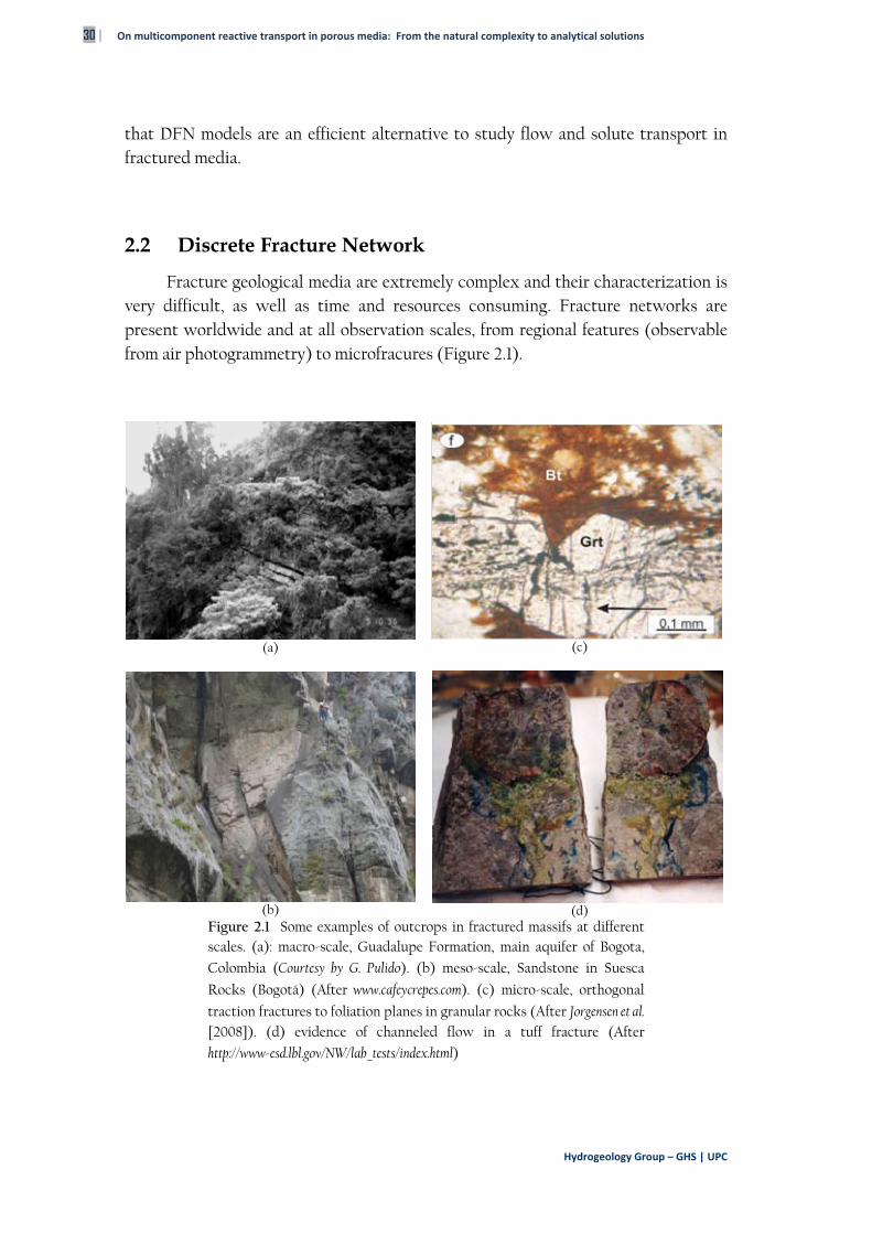
Fracture geological media are extremely complex and their characterization is very difficult, as well as time and resources consuming. Fracture networks are present worldwide and at all observation scales, from regional features (observable from air photogrammetry) to microfracures (Figure 2.1).
(a)
(c)
(b)
(d)
Figure 2.1 Some examples of outcrops in fractured massifs at different scales. (a): macro-scale, Guadalupe Formation, main aquifer of Bogota,
Colombia (Courtesy by G. Pulido). (b) meso-scale, Sandstone in Suesca
Rocks (Bogotá) (After www.cafeycrepes.com). (c) micro-scale, orthogonal
traction fractures to foliation planes in granular rocks (After Jorgensen et al. [2008]). (d) evidence of channeled flow in a tuff fracture (After
http://www-esd.lbl.gov/NW/lab_tests/index.html)
Chapter 2: Inverse modeling in Discrete Fracture Network | 31
Ph. D. Dissertation | L.D. DONADO
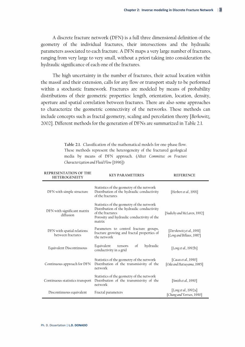
A discrete fracture network (DFN) is a full three dimensional definition of the geometry of the individual fractures, their intersections and the hydraulic parameters associated to each fracture. A DFN maps a very large number of fractures, ranging from very large to very small, without a priori taking into consideration the hydraulic significance of each one of the fractures.
The high uncertainty in the number of fractures, their actual location within the massif and their extension, calls for any flow or transport study to be performed within a stochastic framework. Fractures are modeled by means of probability distributions of their geometric properties: length, orientation, location, density, aperture and spatial correlation between fractures. There are also some approaches to characterize the geometric connectivity of the networks. These methods can
include concepts such as fractal geometry, scaling and percolation theory [Berkowitz, 2002]. Different methods for the generation of DFNs are summarized in Table 2.1.
Table 2.1. Classification of the mathematical models for one-phase flow. These methods represent the heterogeneity of the fractured geological
media by means of DFN approach. (After Committee on Fracture
Characterization and Fluid Flow [1996])
REPRESENTATION OF THE HETEROGENEITY
KEY PARAMETERES REFERENCE
DFN with simple structure Statistics of the geometry of the network Distribution of the hydraulic conductivity of the fractures
[Herbert et al., 1991]
DFN with significant matrix diffusion
Statistics of the geometry of the network Distribution of the hydraulic conductivity of the fractures Porosity and hydraulic conductivity of the matrix
[Sudicky and McLaren, 1992]
DFN with spatial relations between fractures
Parameters to control fracture groups, fracture growing and fractal properties of the network
[Dershowitz et al., 1991] [Long and Billaux, 1987]
Equivalent Discontinuous Equivalent tensors of hydraulic conductivity in a grid [Long et al., 1992b]
Continuous approach for DFN Statistics of the geometry of the network Distribution of the transmisivity of the network
[Cacas et al., 1990] [Oda and Hatsuyama, 1985]
Continuous statistics transport Statistics of the geometry of the network Distribution of the transmisivity of the network
[Smith et al., 1990]
Discontinuous equivalent Fractal parameters [Long et al., 1992a]
[Chang and Yortsos, 1990]
32 | On multicomponent reactive transport in porous media: From the natural complexity to analytical solutions
Hydrogeology Group – GHS | UPC
Adding to the complexity of geometry, each fracture has a characteristic hydraulic behavior. An individual fracture can be modeled as having a constant separation (parallel plate approach), or a variable one. In the former model, a
transmissivity value, T can be defined for each fracture from the cubic law approach;
i.e., T is proportional to b3, where b is the separation among fractures [Bear, 1972;
Witherspoon et al., 1980; Bear and Berkowitz, 1987]. In reality, fracture spacing varies spatially. Then water tends to flow along a small fraction of the fracture, developing
channeling [Tsang and Witherspoon, 1985; Moreno et al., 1988; Moreno and Neretnieks, 1993;
Tsang et al., 1996] which cover small portions of fractures. In some sense, it can be said that water flows through a network of interconnected 1D features. The actual location of these channels and their related hydraulic parameters are flow dependent
and may change with the stress tensor variations [Oda and Hatsuyama, 1985; Durlofsky,
1991; Berkowitz and Scher, 2001].
Analysis of pumping and tracer tests in fracture networks has a number of drawbacks. The number of existing fractures in a system is undefined, since fractures span all scales. The actual number of fractures in a given window can be modeled using fractal concepts, and thus it is necessary to define upper and lower cut-off values to generate realizations of the network with a finite number of fractures. Furthermore, each individual fracture has distinctive hydraulic features. When interpreting tests, it would be necessary to find the estimates of a huge number of hydraulic parameters in an inverse framework. The task would be formidable, but actually the main problem is not the magnitude, but rather the fact that it would be an overparameterized problem.
A different approach is proposed in this work, where the concept of family of fractures is used to reduce significantly the number of parameters to be estimated, so that the problem becomes both stable and solvable. The methodology is presented next.
2.3 Methodology
In this section, we present the applied methodology for modeling flow and transport in geological fracture media by means of a DFN approach. Initially, a description of the generation of fracture networks is shown. This methodology consists on a series of stages that includes characterization of distribution functions for quantity, size, alignment and location of the fractures. A methodology consisting of four modulus (each corresponding to one of the given specified distribution functions) is then implemented sequentially to produce one realization of a fractured system.
Chapter 2: Inverse modeling in Discrete Fracture Network | 33
Ph. D. Dissertation | L.D. DONADO
In the generation process, the sequential concatenation of each one of the modulus must follow the principle of conservation of the fracture density. It means that each new generated fracture network must respect the imposed density (within the simulation domain) and preserving the size distribution function. The result is a synthetic medium, in which additional fractures can be easily added (or removed) to enhance connectivity aspects of the network or to include specific fractures that have been observed or postulated.
2.3.1 Generation of the discrete fracture network
The initial step in our methodology is to define a set of fracture families, defined a priori on the basis of available field observations or on tectonics. Each family is composed by a number of fractures whose location, geometry and
orientation are defined in terms of probability density functions (pdf) supported by
field data such as geological cartography and well logging [see e.g., Nita et al., 2004]. The fracture apertures may also be predefined based on field work or on tectonics
consideration, and also characterized by means of a pdf.
The fracture network is directly generated from these pdf’s, which may or may not be conditional to existing hard data. The usual approach is to select a particular geometry that can be easily parameterized. The usual shape is disks. An individual fracture is thus characterized in a 3D space by a point (location of the center), a length (the radius), three angles (orientation) and a distance (the fracture aperture if
it is considered constant). All these parameters are drawn from the pdf’s either independently or from joint distributions. In the latter case the procedure is to follow a sequential method where parameters are drawn from conditional density functions.
2.3.1.1 Spatial location of the fractures (or simulation support)
In this part of the methodology, the distribution of the fracture centers must be obtained. The model most widely used is Poisson, with constant or variable density, but other models can also be used, such as Gibbs distribution, “birth-death”,
“salvo” or fractal [Geman and Geman, 1984]. Regardless the model selected, it is necessary to provide a set of values to the variables which parameterize them (see Table 2.2). The simulated area can be populated by individual realizations using diverse statistical techniques, including random sampling, genetic algorithms or
simulated annealing [e.g., Ouenes, 2000; Tran and Tran, 2007].
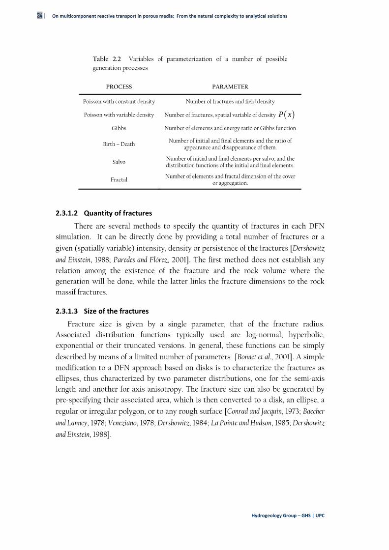
34 | On multicomponent reactive transport in porous media: From the natural complexity to analytical solutions
Hydrogeology Group – GHS | UPC
Table 2.2 Variables of parameterization of a number of possible generation processes
PROCESS PARAMETER
Poisson with constant density Number of fractures and field density
Poisson with variable density Number of fractures, spatial variable of density P x
Gibbs Number of elements and energy ratio or Gibbs function
Birth – Death Number of initial and final elements and the ratio of appearance and disappearance of them.
Salvo Number of initial and final elements per salvo, and the distribution functions of the initial and final elements.
Fractal Number of elements and fractal dimension of the cover or aggregation.
2.3.1.2 Quantity of fractures
There are several methods to specify the quantity of fractures in each DFN simulation. It can be directly done by providing a total number of fractures or a
given (spatially variable) intensity, density or persistence of the fractures [Dershowitz
and Einstein, 1988; Paredes and Flórez, 2001]. The first method does not establish any relation among the existence of the fracture and the rock volume where the generation will be done, while the latter links the fracture dimensions to the rock massif fractures.
2.3.1.3 Size of the fractures
Fracture size is given by a single parameter, that of the fracture radius. Associated distribution functions typically used are log-normal, hyperbolic, exponential or their truncated versions. In general, these functions can be simply
described by means of a limited number of parameters [Bonnet et al., 2001]. A simple modification to a DFN approach based on disks is to characterize the fractures as ellipses, thus characterized by two parameter distributions, one for the semi-axis length and another for axis anisotropy. The fracture size can also be generated by pre-specifying their associated area, which is then converted to a disk, an ellipse, a
regular or irregular polygon, or to any rough surface [Conrad and Jacquin, 1973; Baecher
and Lanney, 1978; Veneziano, 1978; Dershowitz, 1984; La Pointe and Hudson, 1985; Dershowitz
and Einstein, 1988].
Chapter 2: Inverse modeling in Discrete Fracture Network | 35
Ph. D. Dissertation | L.D. DONADO
2.3.1.4 Fracture alignment
Alignment depends on the geological structure mapped on the stereographic
sphere [Pincus, 1951; Rodgers, 1952; Watson, 1966; Jupp and Mardia, 1989]. Several bivariate (direction and dip) distributions could be used here, such as spherical
Fisher, Bingham, or spherical Gauss [Solé-Sugrañes, 1977; Fisher et al., 1987].
2.3.2 From the DFN to a numerical mesh
Once the DFN has been created, the next step corresponds to convert it into a mesh that can be handled by numerical codes. We adopt here a methodology that conceptualizes flow in a fracture network as that of a network of interconnected channels. The methodology we propose is a modification of the channel model
developed by Cacas et al., [1990]. The initial point is to find the conductive fracture network (a subset of the full network). This network is formed by the cluster(s) of fractures that are physically interconnected (not isolated) and also hydraulically connected to the boundaries, so that they are capable of conducting water. Finding the conductive network allows eliminating clusters of fractures which are disconnected from the main fracture skeleton. Removal of these non-conducting fractures allows simplifying the overall computational burden in later stages.
Creating the grid of 1-D elements (channels) is performed in three stages:
(1) Two intersecting disks are connected by two segments, each one having an end (node) located at the disk center. These two points are connected by defining an additional node, located at the intersection of the two fractures (the actual point selected is that minimizing the total length of the segments),Figure 2.2.
(2) Step 1 is repeated for all intersecting disks (Figure 2.3 top) that belong to the interconnected cluster.
(3) Since from step (1) it follows that each element ije generated can be
associated to a particular fracture, it is possible to transfer properties from the fracture to the element. These properties include not only hydraulic parameters, but also the fact that each element can now be associated to one of the fracture families (see Figure 2.3 bottom).
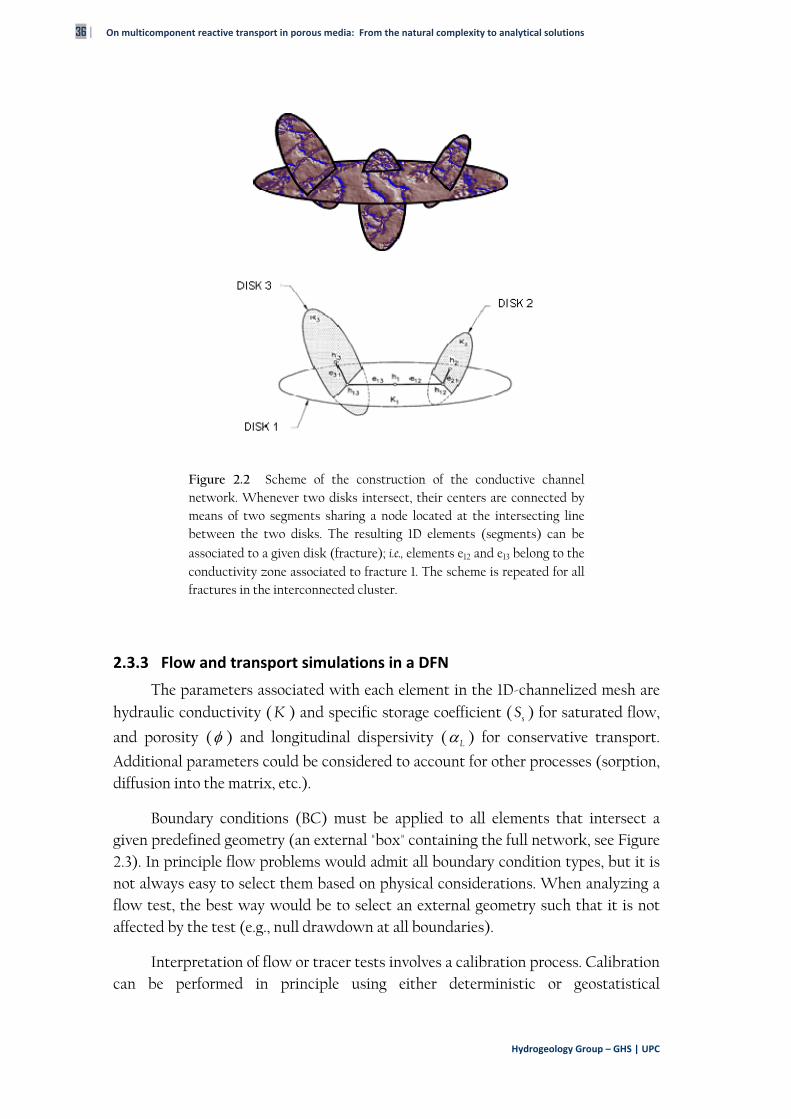
36 | On multicomponent reactive transport in porous media: From the natural complexity to analytical solutions
Hydrogeology Group – GHS | UPC
Figure 2.2 Scheme of the construction of the conductive channel network. Whenever two disks intersect, their centers are connected by means of two segments sharing a node located at the intersecting line between the two disks. The resulting 1D elements (segments) can be
associated to a given disk (fracture); i.e., elements e12 and e13 belong to the conductivity zone associated to fracture 1. The scheme is repeated for all fractures in the interconnected cluster.
2.3.3 Flow and transport simulations in a DFN
The parameters associated with each element in the 1D-channelized mesh are hydraulic conductivity ( K ) and specific storage coefficient ( sS ) for saturated flow,
and porosity ( ) and longitudinal dispersivity ( L ) for conservative transport.
Additional parameters could be considered to account for other processes (sorption, diffusion into the matrix, etc.).
Boundary conditions (BC) must be applied to all elements that intersect a given predefined geometry (an external "box" containing the full network, see Figure 2.3). In principle flow problems would admit all boundary condition types, but it is not always easy to select them based on physical considerations. When analyzing a flow test, the best way would be to select an external geometry such that it is not affected by the test (e.g., null drawdown at all boundaries).
Interpretation of flow or tracer tests involves a calibration process. Calibration can be performed in principle using either deterministic or geostatistical
Chapter 2: Inverse modeling in Discrete Fracture Network | 37
Ph. D. Dissertation | L.D. DONADO
methodologies. Any code that can handle 1D elements in a 3D mesh could be used. Observation points should belong to one of the 1D elements of the conductive network. The way this is ensured is sketched in Figure 2.4. All fractures, intersecting the well are joined to a single node (representing the observation point), creating new 1D elements. Since these elements do not correspond to any given family, an external family must be created (if deemed necessary it could be one new family per observation point).
In order to carry out the inverse problem, we consider that the actual parameter values in each individual element are given by the product of two values: (a) one specific number, based on geometrical and connectivity considerations, and
drawn from a pre-specified pdf, and (b) a scaling factor (termed “family parameter”) which is an unknown value that is the same for all elements associated with a given
family. Only these family parameters are actually calibrated. Thus, the final pdf of a particular parameter in a particular family is just rescaled from the values initially assigned.
This strong reduction in the calibration burden makes it possible to solve demanding transport problems involving different non-conservative processes such as sorption, first-order radioactive decay and matrix diffusion. Whenever one of the processes is incorporated into the conceptual model, some additional parameters arise. These parameters are treated again as the product of an individual parameters for each element times a family parameter to be calibrated.
2.4 Applications to El Berrocal Site
The methodology proposed is now applied to the interpretation of different
tests carried out in El Berrocal Site [D'Alessandro et al., 1995; D'Alessandro et al., 1997a;
D'Alessandro et al., 1997b; Garcia Gutierrez et al., 1997; Rivas et al., 1997], located in the Province of Toledo, Spain (see Figure 2.5).
In this area five fracture families have been characterized according to geomorphologic properties, such as size and orientation, strike and dip. Each family is defined by the number of fractures, and their location, spatial orientation and fracture aperture, each parameter drawn from a predetermined statistical
distribution. Based on a regional model of the site [Rivas et al., 1997], the extension of the simulated block selected was 600 × 600 × 300 m. Detailed methodology about generation of the DFNs is shown in the next section. A total number of 100 equally likely networks were generated by this method.
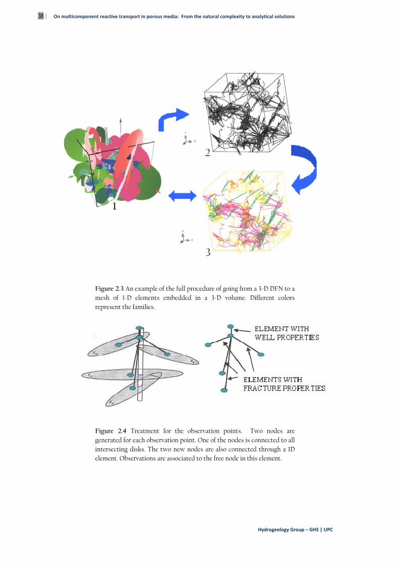
38 | On multicomponent reactive transport in porous media: From the natural complexity to analytical solutions
Hydrogeology Group – GHS | UPC
Figure 2.3 An example of the full procedure of going from a 3-D DFN to a mesh of 1-D elements embedded in a 3-D volume. Different colors represent the families.
Figure 2.4 Treatment for the observation points. Two nodes are generated for each observation point. One of the nodes is connected to all intersecting disks. The two new nodes are also connected through a 1D element. Observations are associated to the free node in this element.
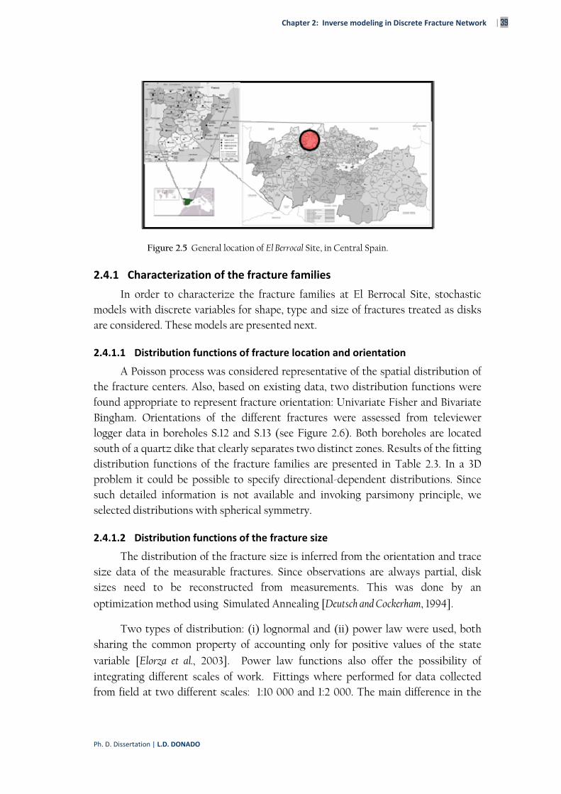
Chapter 2: Inverse modeling in Discrete Fracture Network | 39
Ph. D. Dissertation | L.D. DONADO
Figure 2.5 General location of El Berrocal Site, in Central Spain.
2.4.1 Characterization of the fracture families
In order to characterize the fracture families at El Berrocal Site, stochastic models with discrete variables for shape, type and size of fractures treated as disks are considered. These models are presented next.
2.4.1.1 Distribution functions of fracture location and orientation
A Poisson process was considered representative of the spatial distribution of the fracture centers. Also, based on existing data, two distribution functions were found appropriate to represent fracture orientation: Univariate Fisher and Bivariate Bingham. Orientations of the different fractures were assessed from televiewer logger data in boreholes S.12 and S.13 (see Figure 2.6). Both boreholes are located south of a quartz dike that clearly separates two distinct zones. Results of the fitting distribution functions of the fracture families are presented in Table 2.3. In a 3D problem it could be possible to specify directional-dependent distributions. Since such detailed information is not available and invoking parsimony principle, we selected distributions with spherical symmetry.
2.4.1.2 Distribution functions of the fracture size
The distribution of the fracture size is inferred from the orientation and trace size data of the measurable fractures. Since observations are always partial, disk sizes need to be reconstructed from measurements. This was done by an
optimization method using Simulated Annealing [Deutsch and Cockerham, 1994].
Two types of distribution: (i) lognormal and (ii) power law were used, both sharing the common property of accounting only for positive values of the state
variable [Elorza et al., 2003]. Power law functions also offer the possibility of integrating different scales of work. Fittings where performed for data collected from field at two different scales: 1:10 000 and 1:2 000. The main difference in the
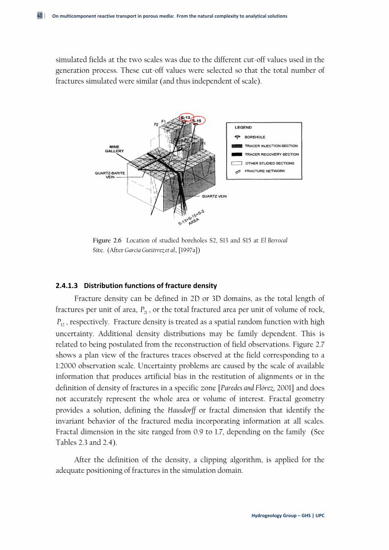
40 | On multicomponent reactive transport in porous media: From the natural complexity to analytical solutions
Hydrogeology Group – GHS | UPC
simulated fields at the two scales was due to the different cut-off values used in the generation process. These cut-off values were selected so that the total number of fractures simulated were similar (and thus independent of scale).
Figure 2.6 Location of studied boreholes S2, S13 and S15 at El Berrocal
Site. (After García Gutiérrez et al., [1997a])
2.4.1.3 Distribution functions of fracture density
Fracture density can be defined in 2D or 3D domains, as the total length of fractures per unit of area, 21P , or the total fractured area per unit of volume of rock,
32P , respectively. Fracture density is treated as a spatial random function with high
uncertainty. Additional density distributions may be family dependent. This is related to being postulated from the reconstruction of field observations. Figure 2.7 shows a plan view of the fractures traces observed at the field corresponding to a 1:2000 observation scale. Uncertainty problems are caused by the scale of available information that produces artificial bias in the restitution of alignments or in the
definition of density of fractures in a specific zone [Paredes and Flórez, 2001] and does not accurately represent the whole area or volume of interest. Fractal geometry
provides a solution, defining the Hausdorff or fractal dimension that identify the invariant behavior of the fractured media incorporating information at all scales. Fractal dimension in the site ranged from 0.9 to 1.7, depending on the family (See Tables 2.3 and 2.4).
After the definition of the density, a clipping algorithm, is applied for the adequate positioning of fractures in the simulation domain.
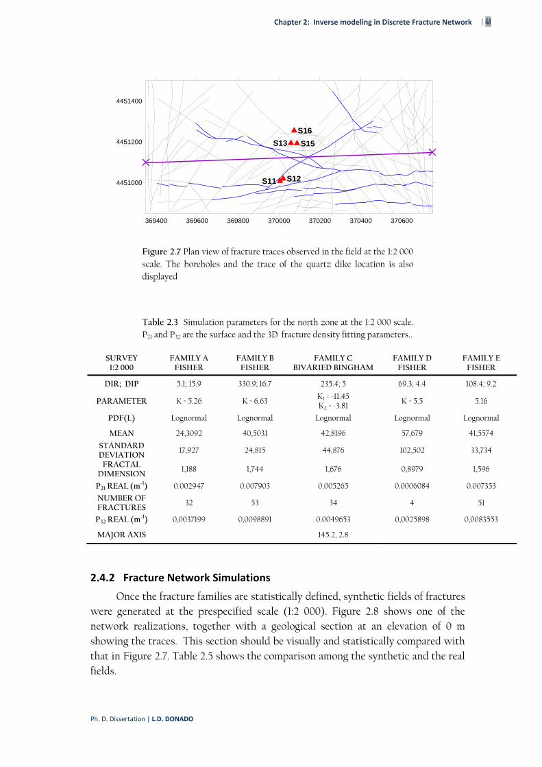
Chapter 2: Inverse modeling in Discrete Fracture Network | 41
Ph. D. Dissertation | L.D. DONADO
369400 369600 369800 370000 370200 370400 370600
4451000
4451200
4451400
S11
S13
S12
S15
S16
Figure 2.7 Plan view of fracture traces observed in the field at the 1:2 000 scale. The boreholes and the trace of the quartz dike location is also displayed
Table 2.3 Simulation parameters for the north zone at the 1:2 000 scale. P21 and P32 are the surface and the 3D fracture density fitting parameters..
SURVEY 1:2 000
FAMILY A FISHER
FAMILY B FISHER
FAMILY C BIVARIED BINGHAM
FAMILY D FISHER
FAMILY E FISHER
DIR; DIP 5.1; 15.9 330.9; 16.7 235.4; 5 69.3; 4.4 108.4; 9.2
PARAMETER K = 5.26 K = 6.63 K1 = -11.45 K2 = -3.81 K = 5.5 5.16
PDF(L) Lognormal Lognormal Lognormal Lognormal Lognormal
MEAN 24,3092 40,5031 42,8196 57,679 41,5574
STANDARD DEVIATION
17,927 24,815 44,876 102,502 33,734
FRACTAL DIMENSION
1,188 1,744 1,676 0,8979 1,596
P21 REAL (m-1) 0.002947 0.007903 0.005265 0.0006084 0.007353
NUMBER OF FRACTURES
32 53 34 4 51
P32 REAL (m-1) 0,0037199 0,0098891 0.0049653 0,0025898 0,0083553
MAJOR AXIS 145.2, 2.8
2.4.2 Fracture Network Simulations
Once the fracture families are statistically defined, synthetic fields of fractures were generated at the prespecified scale (1:2 000). Figure 2.8 shows one of the network realizations, together with a geological section at an elevation of 0 m showing the traces. This section should be visually and statistically compared with that in Figure 2.7. Table 2.5 shows the comparison among the synthetic and the real fields.
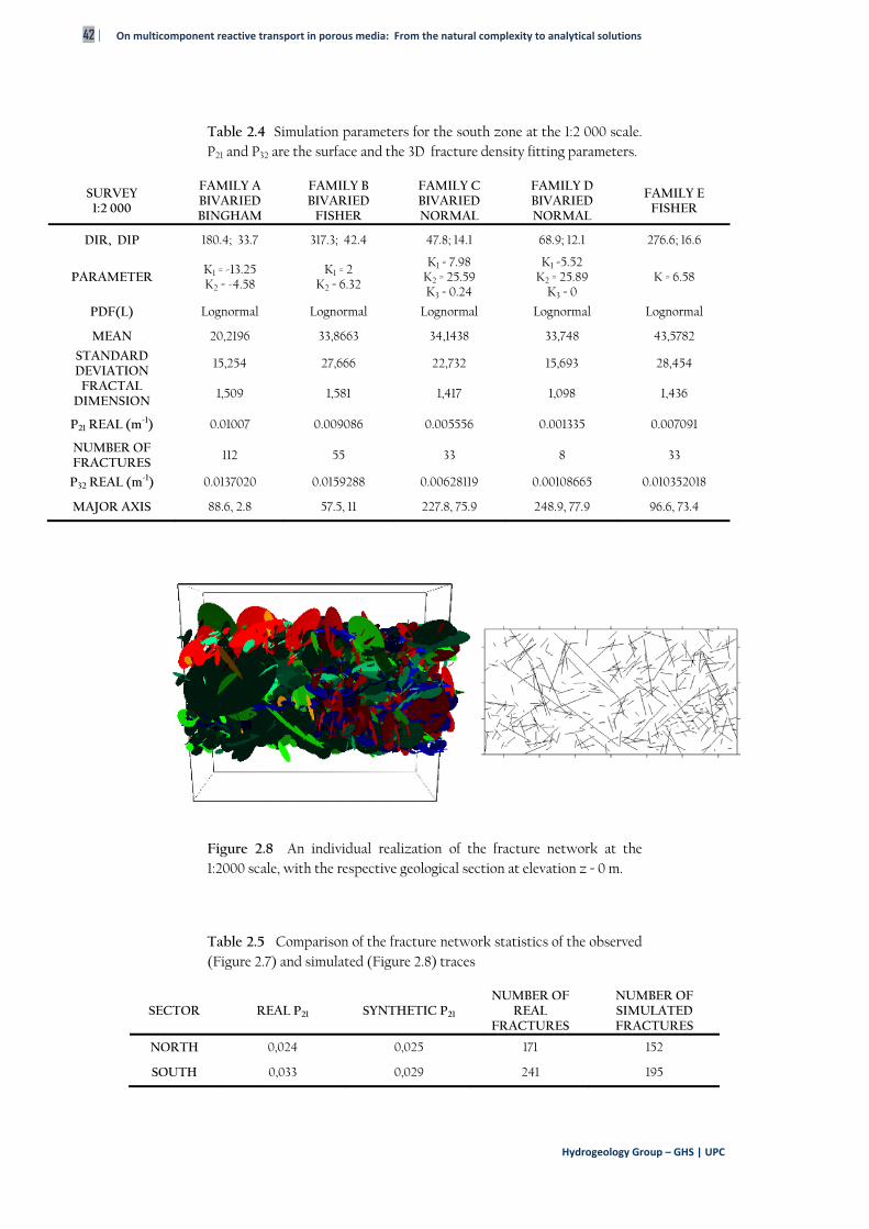
42 | On multicomponent reactive transport in porous media: From the natural complexity to analytical solutions
Hydrogeology Group – GHS | UPC
Table 2.4 Simulation parameters for the south zone at the 1:2 000 scale. P21 and P32 are the surface and the 3D fracture density fitting parameters.
SURVEY 1:2 000
FAMILY A BIVARIED BINGHAM
FAMILY B BIVARIED
FISHER
FAMILY C BIVARIED NORMAL
FAMILY D BIVARIED NORMAL
FAMILY E FISHER
DIR, DIP 180.4; 33.7 317.3; 42.4 47.8; 14.1 68.9; 12.1 276.6; 16.6
PARAMETER K1 = -13.25 K2 = -4.58
K1 = 2 K2 = 6.32
K1 = 7.98 K2 = 25.59 K3 = 0.24
K1 =5.52 K2 = 25.89
K3 = 0 K = 6.58
PDF(L) Lognormal Lognormal Lognormal Lognormal Lognormal
MEAN 20,2196 33,8663 34,1438 33,748 43,5782
STANDARD DEVIATION
15,254 27,666 22,732 15,693 28,454
FRACTAL DIMENSION
1,509 1,581 1,417 1,098 1,436
P21 REAL (m-1) 0.01007 0.009086 0.005556 0.001335 0.007091
NUMBER OF FRACTURES
112 55 33 8 33
P32 REAL (m-1) 0.0137020 0.0159288 0.00628119 0.00108665 0.010352018
MAJOR AXIS 88.6, 2.8 57.5, 11 227.8, 75.9 248.9, 77.9 96.6, 73.4
Figure 2.8 An individual realization of the fracture network at the 1:2000 scale, with the respective geological section at elevation z = 0 m.
Table 2.5 Comparison of the fracture network statistics of the observed (Figure 2.7) and simulated (Figure 2.8) traces
SECTOR REAL P21 SYNTHETIC P21 NUMBER OF
REAL FRACTURES
NUMBER OF SIMULATED FRACTURES
NORTH 0,024 0,025 171 152
SOUTH 0,033 0,029 241 195
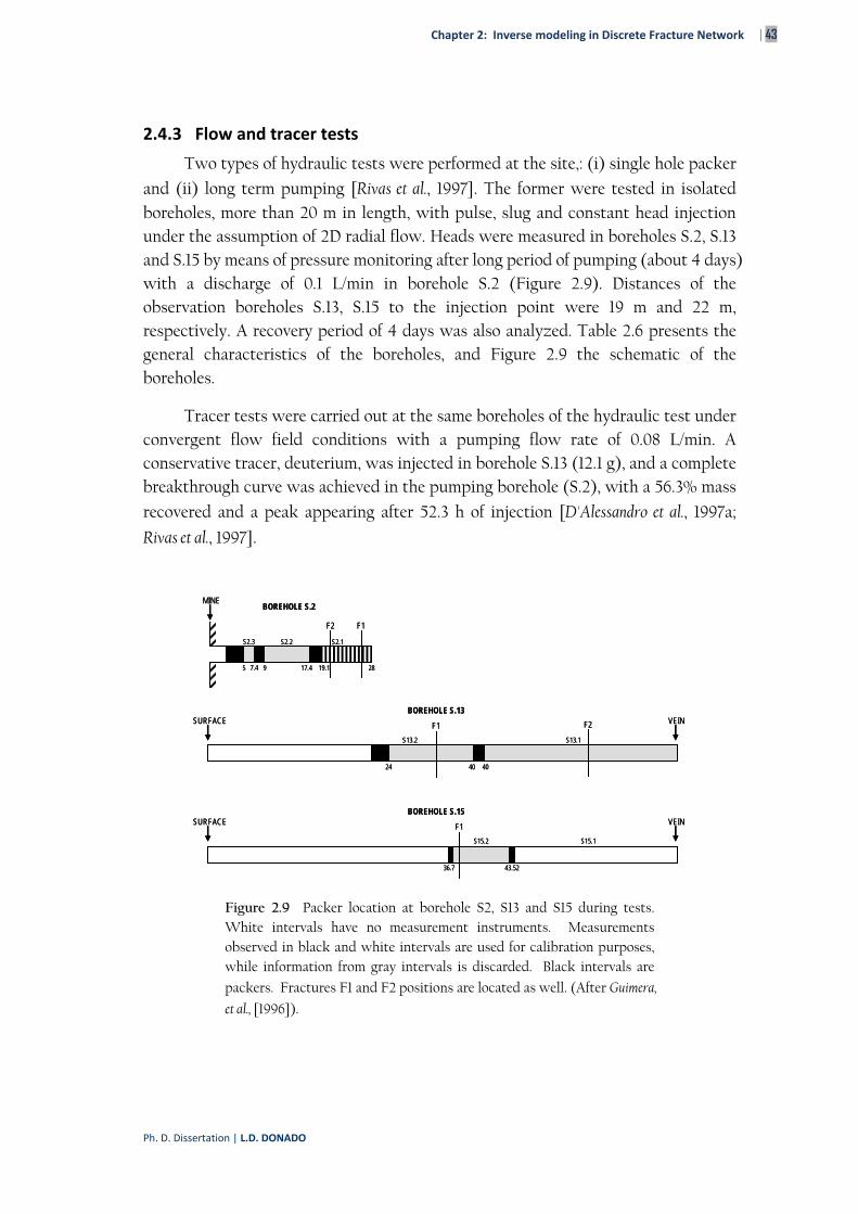
Chapter 2: Inverse modeling in Discrete Fracture Network | 43
Ph. D. Dissertation | L.D. DONADO
2.4.3 Flow and tracer tests
Two types of hydraulic tests were performed at the site,: (i) single hole packer
and (ii) long term pumping [Rivas et al., 1997]. The former were tested in isolated boreholes, more than 20 m in length, with pulse, slug and constant head injection under the assumption of 2D radial flow. Heads were measured in boreholes S.2, S.13 and S.15 by means of pressure monitoring after long period of pumping (about 4 days) with a discharge of 0.1 L/min in borehole S.2 (Figure 2.9). Distances of the observation boreholes S.13, S.15 to the injection point were 19 m and 22 m, respectively. A recovery period of 4 days was also analyzed. Table 2.6 presents the general characteristics of the boreholes, and Figure 2.9 the schematic of the boreholes.
Tracer tests were carried out at the same boreholes of the hydraulic test under convergent flow field conditions with a pumping flow rate of 0.08 L/min. A conservative tracer, deuterium, was injected in borehole S.13 (12.1 g), and a complete breakthrough curve was achieved in the pumping borehole (S.2), with a 56.3% mass
recovered and a peak appearing after 52.3 h of injection [D'Alessandro et al., 1997a;
Rivas et al., 1997].
S2.3 S2.2 S2.1
MINE
F2 F1
5 7.4 9 17.4 19.1 28
BOREHOLE S.2
S2.3 S2.2 S2.1
MINE
F2 F1
5 7.4 9 17.4 19.1 28
BOREHOLE S.2
VEINF1
40
S13.1
F2
S13.2
24 40
SURFACEBOREHOLE S.13
VEINF1
40
S13.1
F2
S13.2
24 40
SURFACEBOREHOLE S.13
VEINF1
36.7
S15.1S15.2
43.52
SURFACEBOREHOLE S.15
VEINF1
36.7
S15.1S15.2
43.52
SURFACEBOREHOLE S.15
Figure 2.9 Packer location at borehole S2, S13 and S15 during tests. White intervals have no measurement instruments. Measurements observed in black and white intervals are used for calibration purposes, while information from gray intervals is discarded. Black intervals are
packers. Fractures F1 and F2 positions are located as well. (After Guimera,
et al., [1996]).
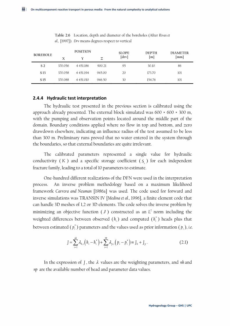
44 | On multicomponent reactive transport in porous media: From the natural complexity to analytical solutions
Hydrogeology Group – GHS | UPC
Table 2.6 Location, depth and diameter of the boreholes (After Rivas et
al., [1997]). Drv means degrees respect to vertical
2.4.4 Hydraulic test interpretation
The hydraulic test presented in the previous section is calibrated using the approach already presented. The external block simulated was 600 × 600 × 300 m, with the pumping and observation points located around the middle part of the domain. Boundary conditions applied where no flow in top and bottom, and zero drawdown elsewhere, indicating an influence radius of the test assumed to be less than 300 m. Preliminary runs proved that no water entered in the system through the boundaries, so that external boundaries are quite irrelevant.
The calibrated parameters represented a single value for hydraulic conductivity ( K ) and a specific storage coefficient (
sS ) for each independent
fracture family, leading to a total of 10 parameters to estimate.
One-hundred different realizations of the DFN were used in the interpretation process. An inverse problem methodology based on a maximum likelihood
framework Carrera and Neuman [1986a] was used. The code used for forward and
inverse simulations was TRANSIN IV [Medina et al., 1996], a finite element code that can handle 3D meshes of 1,2 or 3D elements. The code solves the inverse problem by
minimizing an objective function ( J ) constructed as an 2L norm including the
weighted differences between observed ( ih ) and computed ( *ih ) heads plus that
between estimated ( *ip ) parameters and the values used as prior information ( ip ), i.e.
* *, ,
1 1
npnh
h i i i p i i i h pi i
J h h p p J J . (2.1)
In the expression of J , the values are the weighting parameters, and nh and
np are the available number of head and parameter data values.
BOREHOLE POSITION SLOPE
[drv] DEPTH
[m] DIAMETER
[mm] X Y Z
S 2 370.056 4 451.186 900.21 95 30.10 86
S 13 370.058 4 451.194 945.00 20 173.70 101
S 15 370.088 4 451.010 946.50 30 154.76 101
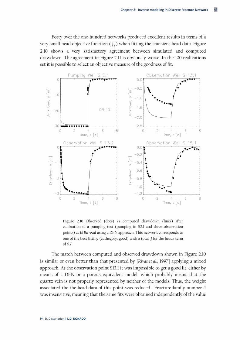
Chapter 2: Inverse modeling in Discrete Fracture Network | 45
Ph. D. Dissertation | L.D. DONADO
Forty over the one-hundred networks produced excellent results in terms of a very small head objective function ( hJ ) when fitting the transient head data. Figure
2.10 shows a very satisfactory agreement between simulated and computed drawdown. The agreement in Figure 2.11 is obviously worse. In the 100 realizations set it is possible to select an objective measure of the goodness of fit.
Figure 2.10 Observed (dots) vs computed drawdown (lines) after calibration of a pumping test (pumping in S2.1 and three observation
points) at El Berrocal using a DFN approach. This network corresponds to
one of the best fitting (cathegory: good) with a total J for the heads term of 6.7.
The match between computed and observed drawdown shown in Figure 2.10
is similar or even better than that presented by [Rivas et al., 1997] applying a mixed approach. At the observation point S13.1 it was impossible to get a good fit, either by means of a DFN or a porous equivalent model, which probably means that the quartz vein is not properly represented by neither of the models. Thus, the weight associated the the head data of this point was reduced. Fracture-family number 4 was insensitive, meaning that the same fits were obtained independently of the value
46 | On multicomponent reactive transport in porous media: From the natural complexity to analytical solutions
Hydrogeology Group – GHS | UPC
used for this particular zone. This is an indication that in the vicinity of the test area very few, if any, of the conducting elements belongs to that particular family.
Results were divided in four groups according to their hJ value. Those groups
were: good (0 to 10), fair (10 to 20), bad (20 to 50) and unfittable (greatest than 50). Around 40% of the networks provided values below 10, and those were selected as potential candidates for tracer test interpretations, that will be presented in the next subsection.
Figure 2.11 Best fit for a given fracture network realization. This network
is classified as bad in terms of calibration purposes. In this case J for
heads only is 34.85 (compare it with that of the previous figure).
2.4.5 Tracer test interpretation
The proposed methodology was extended to transport analysis in the forty networks, where flow could be calibrated with a good fitting to the observed data, thus providing a good to excellent fit of the hydraulic test. A convergent tracer test involving the same piezometers was then analyzed. This test was carried out with an
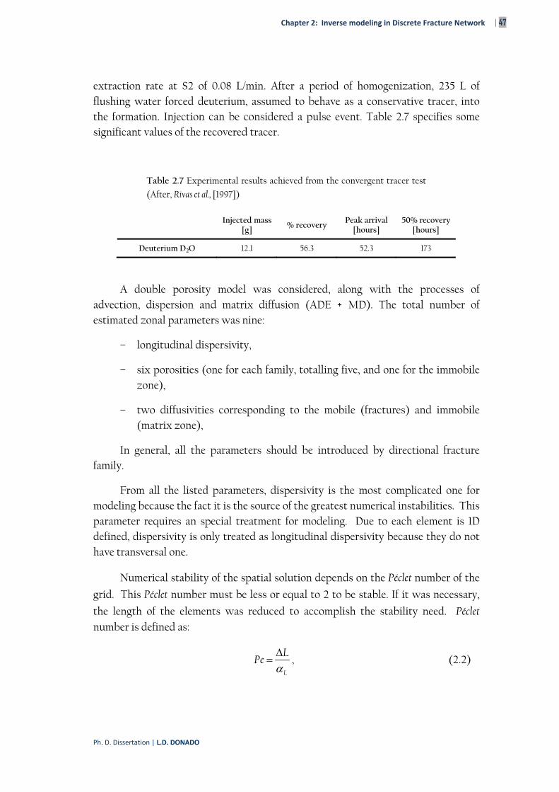
Chapter 2: Inverse modeling in Discrete Fracture Network | 47
Ph. D. Dissertation | L.D. DONADO
extraction rate at S2 of 0.08 L/min. After a period of homogenization, 235 L of flushing water forced deuterium, assumed to behave as a conservative tracer, into the formation. Injection can be considered a pulse event. Table 2.7 specifies some significant values of the recovered tracer.
Table 2.7 Experimental results achieved from the convergent tracer test
(After, Rivas et al., [1997])
Injected mass
[g] % recovery
Peak arrival [hours]
50% recovery [hours]
Deuterium D2O 12.1 56.3 52.3 173
A double porosity model was considered, along with the processes of advection, dispersion and matrix diffusion (ADE + MD). The total number of estimated zonal parameters was nine:
– longitudinal dispersivity,
– six porosities (one for each family, totalling five, and one for the immobile zone),
– two diffusivities corresponding to the mobile (fractures) and immobile (matrix zone),
In general, all the parameters should be introduced by directional fracture family.
From all the listed parameters, dispersivity is the most complicated one for modeling because the fact it is the source of the greatest numerical instabilities. This parameter requires an special treatment for modeling. Due to each element is 1D defined, dispersivity is only treated as longitudinal dispersivity because they do not have transversal one.
Numerical stability of the spatial solution depends on the Péclet number of the
grid. This Péclet number must be less or equal to 2 to be stable. If it was necessary,
the length of the elements was reduced to accomplish the stability need. Péclet number is defined as:
L
LPe
, (2.2)
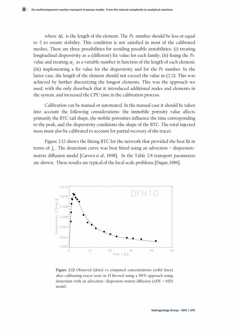
48 | On multicomponent reactive transport in porous media: From the natural complexity to analytical solutions
Hydrogeology Group – GHS | UPC
where L is the length of the element. The Pe number should be less or equal to 2 to ensure stability. This condition is not satisfied in most of the calibrated meshes. There are three possibilities for avoiding possible instabilities: (i) treating longitudinal dispersivity as a (different) fix value for each family; (ii) fixing the Pe value and treating L as a variable number in function of the length of each element;
(iii) implementing a fix value for the dispersivity and for the Pe number. In the latter case, the length of the element should not exceed the value in (2.2). This was achieved by further discretizing the longest elements. This was the approach we used, with the only drawback that it introduced additional nodes and elements in the system, and increased the CPU time in the calibration process.
Calibration can be manual or automated. In the manual case it should be taken into account the following considerations: the immobile porosity value affects primarily the BTC tail shape, the mobile porosities influence the time corresponding to the peak, and the dispersivity conditions the shape of the BTC. The total injected mass must also be calibrated to account for partial recovery of the tracer.
Figure 2.12 shows the fitting BTC for the network that provided the best fit in terms of hJ . The deuterium curve was best fitted using an advection – dispersion–
matrix diffusion model [Carrera et al., 1998]. In the Table 2.8 transport parameters
are shown. These results are typical of the local scale problems [Dagan, 1986].
Figure 2.12 Observed (dots) vs computed concentrations (solid lines)
after calibrating tracer tests in El Berrocal using a DFN approach using deuterium with an advection– dispersion–matrix diffusion (ADE + MD) model.
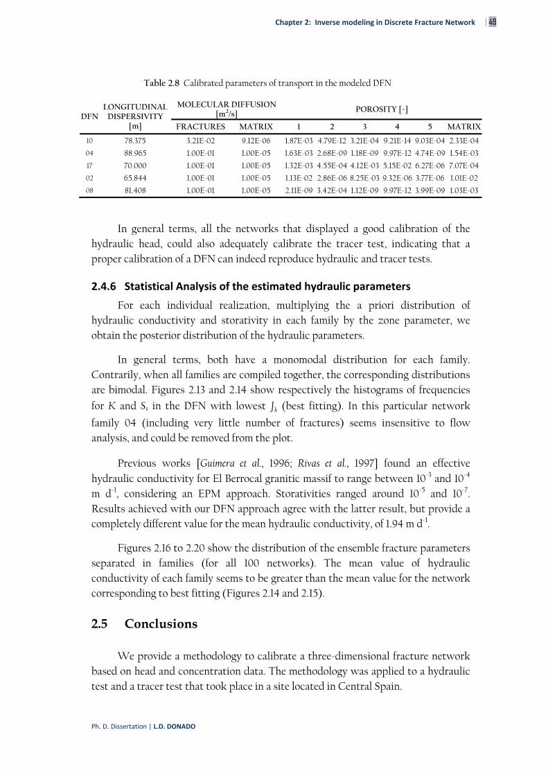
Chapter 2: Inverse modeling in Discrete Fracture Network | 49
Ph. D. Dissertation | L.D. DONADO
Table 2.8 Calibrated parameters of transport in the modeled DFN
DFN LONGITUDINAL
DISPERSIVITY [m]
MOLECULAR DIFFUSION [m2/s]
POROSITY [-]
FRACTURES MATRIX 1 2 3 4 5 MATRIX
10 78.375 3.21E-02 9.12E-06 1.87E-03 4.79E-12 3.21E-04 9.21E-14 9.03E-04 2.33E-04
04 88.965 1.00E-01 1.00E-05 1.63E-03 2.68E-09 1.18E-09 9.97E-12 4.74E-09 1.54E-03
17 70.000 1.00E-01 1.00E-05 1.32E-03 4.55E-04 4.12E-03 5.15E-02 6.27E-06 7.07E-04
02 65.844 1.00E-01 1.00E-05 1.13E-02 2.86E-06 8.25E-03 9.32E-06 3.77E-06 1.01E-02
08 81.408 1.00E-01 1.00E-05 2.11E-09 3.42E-04 1.12E-09 9.97E-12 3.99E-09 1.03E-03
In general terms, all the networks that displayed a good calibration of the hydraulic head, could also adequately calibrate the tracer test, indicating that a proper calibration of a DFN can indeed reproduce hydraulic and tracer tests.
2.4.6 Statistical Analysis of the estimated hydraulic parameters
For each individual realization, multiplying the a priori distribution of hydraulic conductivity and storativity in each family by the zone parameter, we obtain the posterior distribution of the hydraulic parameters.
In general terms, both have a monomodal distribution for each family. Contrarily, when all families are compiled together, the corresponding distributions are bimodal. Figures 2.13 and 2.14 show respectively the histograms of frequencies
for K and Ss in the DFN with lowest hJ (best fitting). In this particular network
family 04 (including very little number of fractures) seems insensitive to flow analysis, and could be removed from the plot.
Previous works [Guimera et al., 1996; Rivas et al., 1997] found an effective hydraulic conductivity for El Berrocal granitic massif to range between 10-3 and 10-4 m d-1, considering an EPM approach. Storativities ranged around 10-5 and 10-7. Results achieved with our DFN approach agree with the latter result, but provide a completely different value for the mean hydraulic conductivity, of 1.94 m d-1.
Figures 2.16 to 2.20 show the distribution of the ensemble fracture parameters separated in families (for all 100 networks). The mean value of hydraulic conductivity of each family seems to be greater than the mean value for the network corresponding to best fitting (Figures 2.14 and 2.15).
2.5 Conclusions
We provide a methodology to calibrate a three-dimensional fracture network based on head and concentration data. The methodology was applied to a hydraulic test and a tracer test that took place in a site located in Central Spain.
50 | On multicomponent reactive transport in porous media: From the natural complexity to analytical solutions
Hydrogeology Group – GHS | UPC
One hundred different realizations of a DFN were used in the calibration process. Eighty per cent (80%) of the networks analyzed presented acceptable
agreement with observed drawdowns (i.e., a low value of the objective functions for heads). Furthermore, about 30% of those provide an excellent fitting in terms of heads. Fittings are comparable with, and in some cases better, than those obtained by means of an approach based on an equivalent porous media with embedded fractures. The methodology allows one to calibrate a relatively small number of parameters, making the calibration process possible. The actual fitted parameters
(zonal K and Ss values) vary with each simulation. Families that do not contribute to flow can be detected by this method. The tracer test interpretation allows additional parameters to be estimated, such as porosity and dispersivity, along with the porosity and dispersion coefficient of the immobile zone if a double porosity model is adopted.
In conclusion, the methodology presented allows calibrating the relevant parameters corresponding to a DFN. The definite advantage of the method is that the DFN simulated is not unique, so this methodology can be easily and immediately applied in a geostatistical framework, thus making it easier to give physical meaning to the calibrated values.
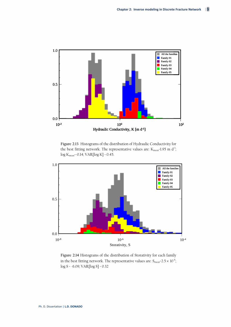
Chapter 2: Inverse modeling in Discrete Fracture Network | 51
Ph. D. Dissertation | L.D. DONADO
All the families
Family 02
Family 03Family 04
Family 05
Family 01
0.0
0.5
1.0
10-2 100 102
Hydraulic Conductivity, K [m d-1]
All the families
Family 02
Family 03Family 04
Family 05
Family 01
All the families
Family 02
Family 03Family 04
Family 05
Family 01
0.0
0.5
1.0
10-2 100 102
Hydraulic Conductivity, K [m d-1]10-2 100 102
Hydraulic Conductivity, K [m d-1]
Figure 2.13 Histograms of the distribution of Hydraulic Conductivity for the best fitting network. The representative values are: Kmean=1.95 m d-1; log Kmean=-0.14; VAR[log K] = 0.45.
All the families
Family 02
Family 03Family 04
Family 05
Family 01
All the families
Family 02
Family 03Family 04
Family 05
Family 01
0.0
0.5
1.0
10-8 10-6 10-4
Storativity, S
Figure 2.14 Histograms of the distribution of Storativity for each family
in the best fitting network. The representative values are: Smean=2.5 10-6; log S = -6.09; VAR[log S] = 0.32
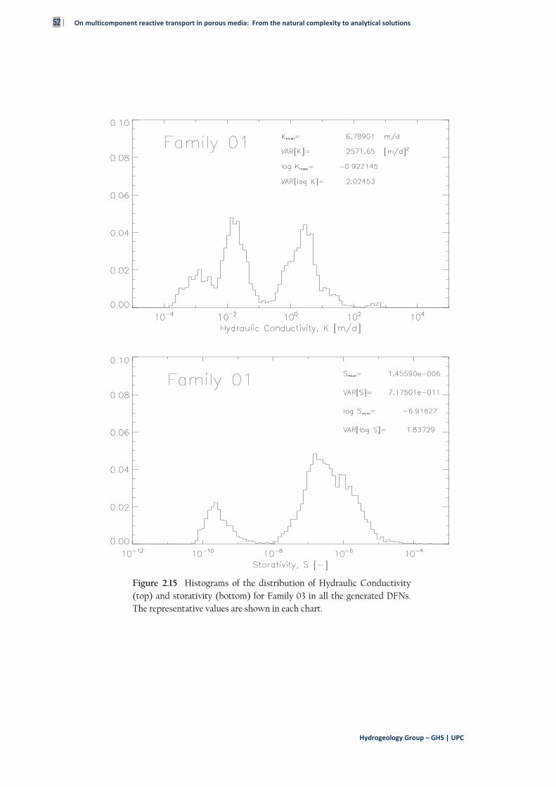
52 | On multicomponent reactive transport in porous media: From the natural complexity to analytical solutions
Hydrogeology Group – GHS | UPC
Figure 2.15 Histograms of the distribution of Hydraulic Conductivity (top) and storativity (bottom) for Family 03 in all the generated DFNs. The representative values are shown in each chart.
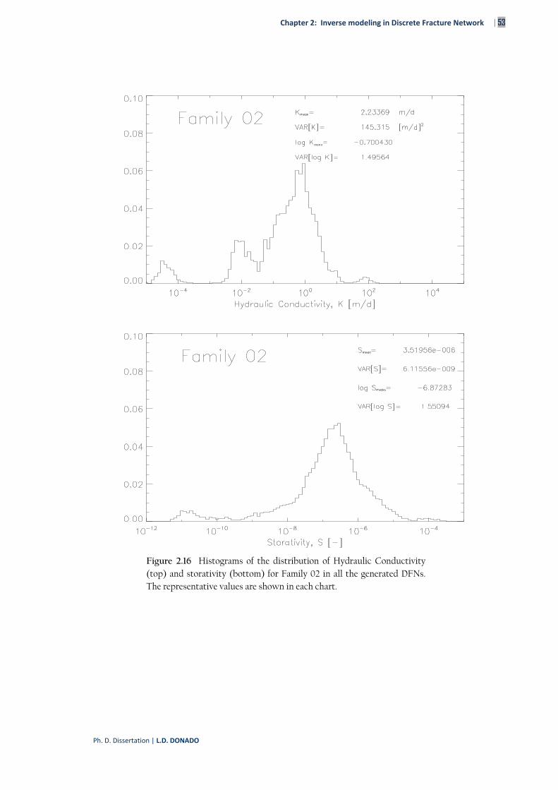
Chapter 2: Inverse modeling in Discrete Fracture Network | 53
Ph. D. Dissertation | L.D. DONADO
Figure 2.16 Histograms of the distribution of Hydraulic Conductivity (top) and storativity (bottom) for Family 02 in all the generated DFNs. The representative values are shown in each chart.
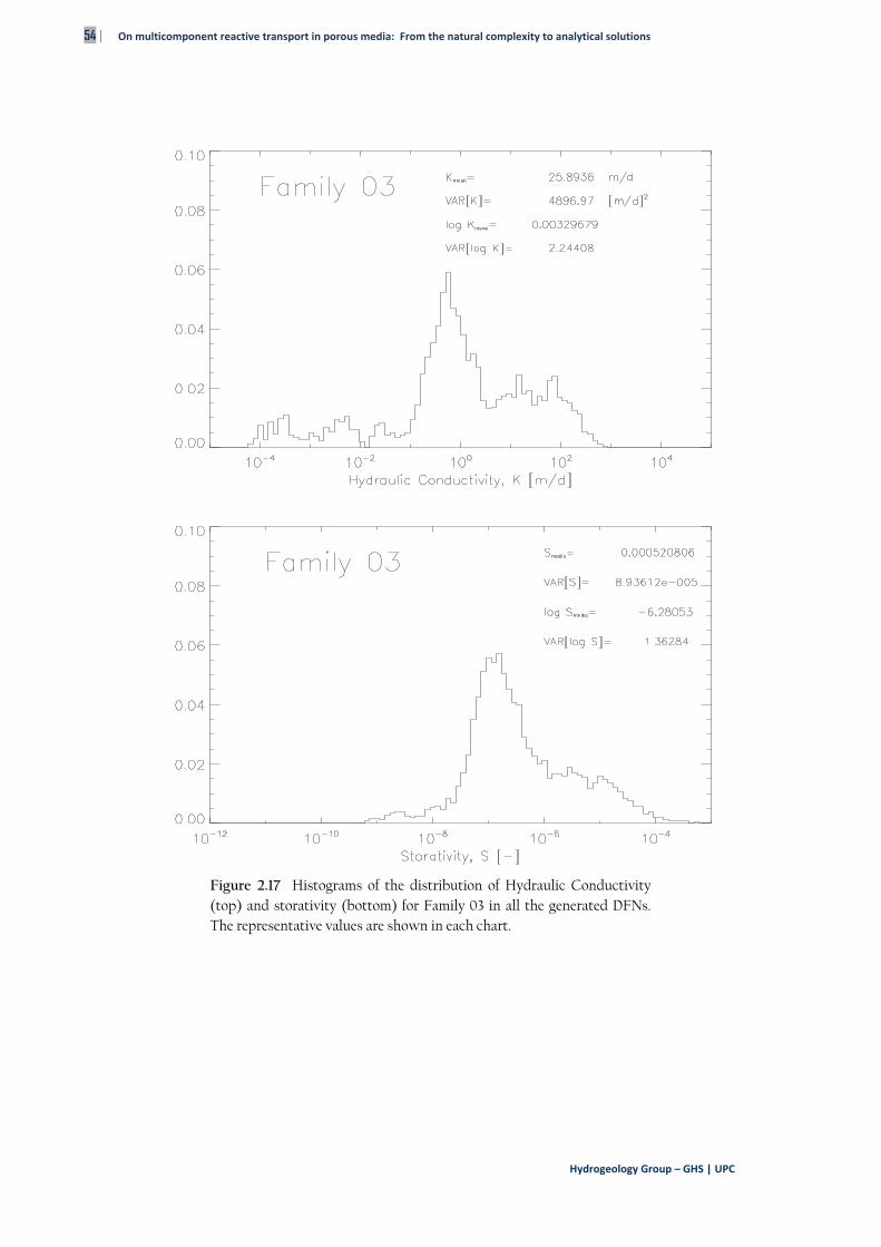
54 | On multicomponent reactive transport in porous media: From the natural complexity to analytical solutions
Hydrogeology Group – GHS | UPC
Figure 2.17 Histograms of the distribution of Hydraulic Conductivity (top) and storativity (bottom) for Family 03 in all the generated DFNs. The representative values are shown in each chart.
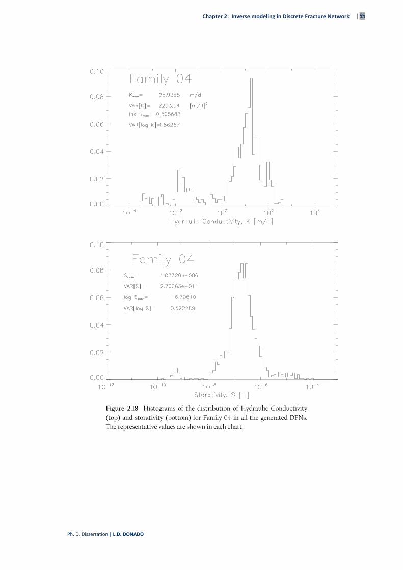
Chapter 2: Inverse modeling in Discrete Fracture Network | 55
Ph. D. Dissertation | L.D. DONADO
Figure 2.18 Histograms of the distribution of Hydraulic Conductivity (top) and storativity (bottom) for Family 04 in all the generated DFNs. The representative values are shown in each chart.
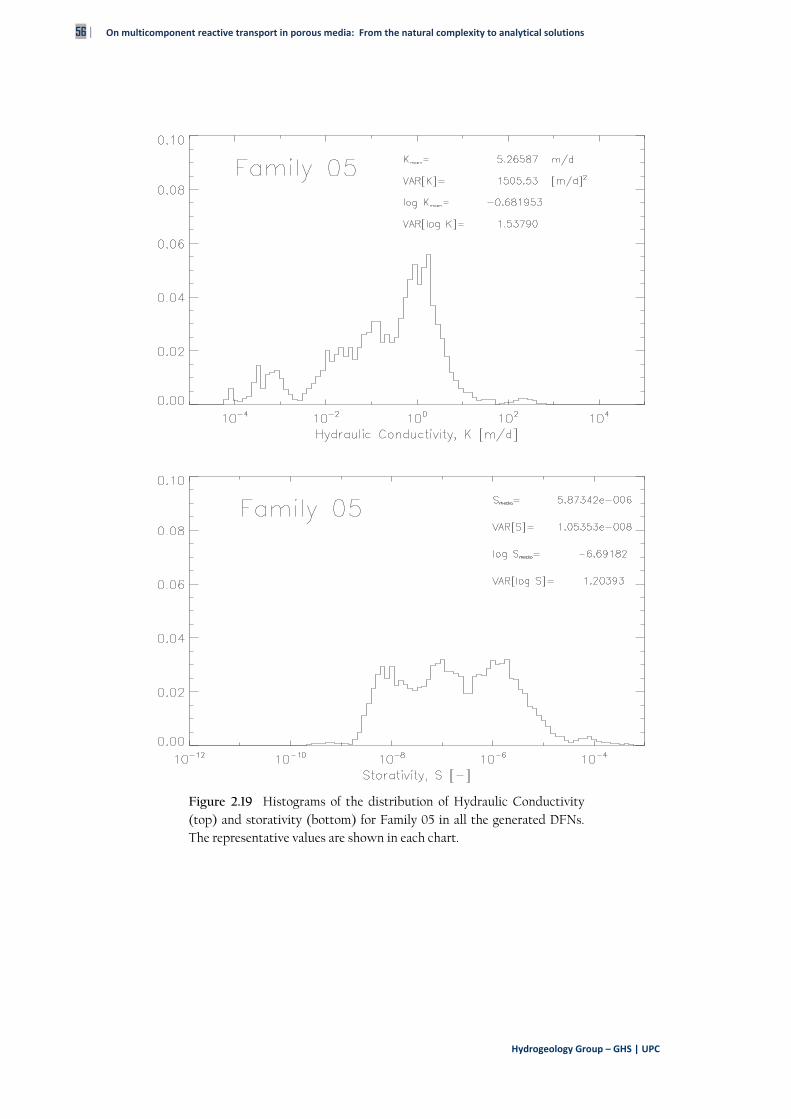
56 | On multicomponent reactive transport in porous media: From the natural complexity to analytical solutions
Hydrogeology Group – GHS | UPC
Figure 2.19 Histograms of the distribution of Hydraulic Conductivity (top) and storativity (bottom) for Family 05 in all the generated DFNs. The representative values are shown in each chart.
chapter
On multicomponent reactive transport in porous media: From the natural complexity to analytical solutions

(This page intentionally left blank.)
Chapter 3: Reaction rates for mixing‐controlled reaction in multi‐continuum media | 57
Ph. D. Dissertation | L.D. DONADO
Chapter 3
Reaction rates for mixing‐controlled reaction in multi‐continuum media
3 REACTION RATES FOR MIXING‐
CONTROLLED REACTION IN MULTI‐
CONTINUUM MEDIA
3.1 Introduction
Reactive transport through natural permeable media incorporates complexity at different levels. On the one hand, aquifers are heterogeneous in terms of hydraulic parameters. On the other hand, reactions may require incorporating a large number of aqueous and solid species and a variety of reaction types. Coupling these two complexities is not trivial. Hence, multicomponent reactive transport has been traditionally modeled by means of the advection-dispersion equation (ADE) with
additional terms to represent reactions [e.g., Cederberg et al., 1985; Rubin, 1990; Wang
and VanCappellen, 1996]. These terms can include all kinds of reactions and affect hydraulic properties (e.g. porosity or hydraulic conductivity), causing the problem to be coupled and difficult.
Hence, efforts have concentrated on developing solution methodologies with
emphasis on accurate representation of multicomponent reactions. However, Rezaei
58 | On multicomponent reactive transport in porous media: From the natural complexity to analytical solutions
Hydrogeology Group – GHS | UPC
et al. [2005] showed that the rate, location and occurrence conditions for equilibrium reactions may be controlled more by transport, specifically mixing, than by chemistry. This is true not only for equilibrium reactions but also for fast
degradation reactions [see Borden and Bedient, 1986; Cirpka and Valocchi, 2007]. In fact,
De Simoni et al. [2005] derived an equation for equilibrium reaction rates that expresses this dependence explicitly. In this expression reaction rate is proportional
to a mixing factor as expressed by a term similar to the dilution index [Kitanidis,
1994]. This point is further stressed by De Simoni et al. [2007], who write reaction rates using the dilution index in terms of mixing ratios. Aside, from the fact that this may be computationally advantageous whenever the number of end-member waters is smaller than the number of components, it illustrates that mixing is indeed what controls many chemical reactions.
The main difficulty in dealing with reactive transport through heterogeneous media lies precisely on how to characterize mixing. Mixing has been traditionally described by dispersion coefficients. In fact, macrodispersion coefficients account
for the effect of heterogeneity [Gelhar and Axness, 1983; Dagan, 1986; Neuman et al., 1987]. However macrodispersion measures spreading (rate of growth of plume moments) rather than mixing. Therefore, it is inadequate for simulating reactive transport. As a result, thorough analyses of the effect of heterogeneity on reactive transport have been restricted to explicitly simulated variability of hydraulic conductivity and use
of local dispersion. Such is the case of Molz and Widdowson [1988] or Fernandez-Garcia et
al., [2008], who used a stratified medium, or MacQuarrie and Sudicky [1990] and Luo et
al. [2008] who considered a random field. These kinds of approaches yield insight into the effect of heterogeneity. However, they are hard to generalize and cumbersome in practice.
It is clear that a simplified transport equation discriminating between mixing and spreading is needed. Attempts along this line have been made in what can be termed effective dynamics approximations. Most of these consist of the inclusion of an immobile region in semi-phenomenological approaches that lead to methods such
as the memory function [Carrera et al., 1998], multi-rate mass transfer (MRMT)
[Haggerty and Gorelick, 1995; Wang et al., 2005], or continuous time random walk
(CTRW) [e.g., Berkowitz and Scher, 1998; Berkowitz et al., 2006]. All these methodologies share the concept that if the medium is homogenized, there is a need to incorporate a term in the governing equation that accounts for memory of the micro-scale heterogeneities that solutes have sampled along their path. These memory effects influence transport at the large scale.
So far, effective dynamics have been explored in the literature only for solutes that are either conservative or that sorb reversibly to the mineral phase. While
Chapter 3: Reaction rates for mixing‐controlled reaction in multi‐continuum media | 59
Ph. D. Dissertation | L.D. DONADO
sorption reactions can be of interest for many environmental reactions, it is also true that other type of reactions must be incorporated in the analysis in order to have a complete picture of the effect of heterogeneity upon multicomponent reactive transport. Moreover, the fact that they explicitly discriminate between mixing and spreading makes them ideally suited for reactive transport. In fact, these models make an explicit attempt at representing the complexity of transport at the pore
scale [Lichtner, 1985]. The fact that effective dynamics approximations incorporate pore scale complexity and a clear discrimination between mixing and spreading is hopeful, but not sufficient. To be accurate, these approximations would have to accurately represent mixing, which to date has not been proven. What these approximations yield, after calibrations is a proper reproduction of the pdf of travel
times [Luo and Cirpka, 2008]. This is necessary for reproducing mixing, but not sufficient. One can envision cases where a given pdf is the result of mixing as well as the superposition of nearly independent flow tubes. It is clear that further research is needed to ascertain under which circumstances mixing is properly reproduced. One way to do so would be by comparing breakthrough curves of reacting and conservative tracers. To this end, we need to have analytical solutions for multicomponent reactive transport using effective dynamics approximations.
Analytical solutions for rather general multi-component reactive transport
problems are available [e.g., Sun et al., 1999; Clement, 2001; Serrano, 2003; Quezada et al.,
2004; Sun et al., 2004; De Simoni et al., 2005; Werth et al., 2006; De Simoni et al., 2007]. However, these analytical procedures are restricted to physical and chemical homogeneity. With the notable exception of adsorption and linear decay processes, few published papers address the use of analytical methods for solving reactive transport problems in heterogeneous media. This is ironic as heterogeneity is arguably the most singular characteristic of natural aquifers. Attempts at dealing
with heterogeneity through perturbation approaches [Miralles-Wilhelm et al., 1998; Luo
et al., 2008] have met with limited success. Certainly, no solution is available for multicomponent reactive transport using effective dynamics approximations. The main reason is that effective dynamics methods are non-local, that is, they work with concentration distributions rather than local values, which are the ones needed for simulating reactions.
In this work, we deal with heterogeneity in terms of an effective transport model using the multi rate mass transfer approach (MRMT), which represents the heterogeneous media as a multi continuum of a mobile and several immobile regions.
Solute is exchanged between these regions by linear kinetic mass transfer [Haggerty et
al., 2000]. The MRMT approach is equivalent to a certain implementation of
continuous time random walks (CTRW) [Dentz and Berkowitz, 2003]. We prove the
60 | On multicomponent reactive transport in porous media: From the natural complexity to analytical solutions
Hydrogeology Group – GHS | UPC
impact of mass transfer on reactive transport in terms of explicit expressions for the reaction rates in the mobile and immobile regions.
3.2 Mathematical Model
A multicomponent reactive transport problem is defined by (i) the chemical system, including the aqueous and mineral species involved and the reactions taking place amongst them and (ii) the transport model defined in terms of mass balance equations. In this work all reactions are assumed to be in chemical equilibrium; that is, the characteristic reaction time is much smaller than the characteristic diffusive time.
We first write the full multicomponent reactive transport problem in terms of chemical components. Then we extend it to multicontinuum media. The resulting system yields a suite of uncoupled conservative transport problems. Reaction rates can then be written explicitly in terms of the components and the prespecified memory function.
3.2.1 Chemical system
The main assumption in this work is that all reactions are in chemical equilibrium. Thus, they can be represented by means of mass action laws, written
here in matrix format [e.g., Saaltink et al., 1998]:
log logS c K , (3.1)
where S is the stoichiometric matrix, c is the vector of species concentrations (mass of species per unit volume of fluid), and K contains the equilibrium constants for all reactions involved. Mass action laws hold for both homogeneous (i.e. all reactants in the same phase) and heterogeneous (some reactants in aqueous and some in solid phases) reactions.
Components can be defined as linear combinations of species, that remain
unaffected by equilibrium reactions [Saaltink et al., 1998]. This linear relation can be written as
u Uc , (3.2)
where u is the vector of components, and U is termed the components matrix, satisfying
0TUS . (3.3)
Chapter 3: Reaction rates for mixing‐controlled reaction in multi‐continuum media | 61
Ph. D. Dissertation | L.D. DONADO
Most methodologies to solve geochemical reactive transport problems are based on posing and solving the problem in the component space. Concentrations can then be obtained from speciation calculations. These consist of solving (3.1) and (3.2) for c given u .
3.2.2 Reactive transport in single continuum media
The governing mass balance equations can be written in compact form as
, , ' ,tt L t tt
c x M c x f x , (3.4)
where is porosity; M is a diagonal matrix with terms equal to either unity
for aqueous species, or zero for minerals; and 'f is a sink/source term (mass of species per unit volume of aquifer and unit time). This last term accounts for the mass of a given species that is produced or lost due to chemical reactions (e.g., precipitation will be a net loss of mass of each of the reacting species, and a gain in
the mineral species). The linear operator tL c accounts for advection and
diffusion/dispersion
, , · ,tL t t t c x q c x D c x , (3.5)
q being Darcy’s flux and D the dispersion tensor. The sink/source term 'f in
(3.4) is a linear combination of reaction rates, since a single species can be involved in more than one reaction with different stoichiometric coefficients. Defining r as
the vector of reaction rates, it is possible to write [e.g., Saaltink et al., 1998]
' 'Tf S r . (3.6)
Notice that this formulation implicitly assumes that all species are subject to identical transport processes, which is clearly true for advection and mechanical dispersion, but could be argued for molecular diffusion and porosity.
3.2.3 Reactive transport in multicontinuum media
Solute transport through heterogeneous media faces difficulties as it makes it impossible to accurately know the spatial distribution of q . This implies that any
solution of (3.4) will lead to uncertain c values. Several approaches, either analytical or numerical, are available in the literature to tackle this problem. Analytical approaches to transport problems can be classified broadly into two groups: perturbation approaches and effective dynamics. In the former, the main idea is not
62 | On multicomponent reactive transport in porous media: From the natural complexity to analytical solutions
Hydrogeology Group – GHS | UPC
to reproduce concentration values at the local scale, but rather to find their low order statistical moments (typically, expected value and variance-covariance of concentrations). The process usually involves ensemble averaging, which smoothes out spatial fluctuations. As a result, transport parameters derived from conservative transport using these methods cannot be used for simulating mixing driven reactive transport. In the latter group, the goal is to find an effective equation to substitute the ADE approach.
Several alternatives can be used to model effective dynamics (FADE [Benson et
al., 2000a; Cushman and Ginn, 2000]; CTRW [Berkowitz and Scher, 1995; Berkowitz et al.,
2006]; MRMT [Haggerty and Gorelick, 1995; Carrera et al., 1998; Lawrence et al., 2002]). Most of them include non-local terms that hinder reactive transport calculations. However, some of these formulations can be localized using multicontinuum methods. In essence, these consist of viewing the medium as the superposition of a mobile and an ensemble of immobile continua. These regions interact so that solute mass is transferred between the mobile and each of the immobile regions. This model originated in the physical-chemistry literature where it was used to model photon
trapping [e.g., Schmidlin, 1977] or non-instantaneous adsorption in batch reactors [e.g.,
Connaughton et al., 1993] using a finite number of immobile phases. The model (usually. but non-uniquely, termed Multi Rate Mass Transfer -MRMT- model), was later
coupled to transport [Haggerty and Gorelick, 1995] and further extended to a
continuous suite of immobile phases [Haggerty and Gorelick, 1998]. The resulting
breakthrough curves are analogous to those measured in the field (i.e., in physically heterogeneous media). This prompted several authors to propose similar models as
an alternative model for transport through heterogeneous media [Berkowitz and Scher,
1998; Carrera et al., 1998; Haggerty et al., 2001]. Sanchez-Vila and Carrera [2004] demonstrated that in the limit of large distances a diffusive problem provides approximately the same statistical moments as a macrodispersive model in a stationary field, thus extending the range of validity of the formulation to large
scales. Dentz and Berkowitz [2003] showed the equivalence between CTRW and MRMT models for particular cases.
Multicontinuum models for conservative species are fully defined by the distribution of , first order exchange rates between the mobile and the immobile
continua. This distribution, f , can be seen as the fraction of immobile sites that
transfer mass at a given rate [T-1]. This distribution is directly related to the
better known concept of memory function [Carrera et al., 1998; Haggerty et al., 2000], by
Chapter 3: Reaction rates for mixing‐controlled reaction in multi‐continuum media | 63
Ph. D. Dissertation | L.D. DONADO
0
tg t f e d
, (3.7)
Solute mass is distributed between mobile and immobile regions which
concentrations ,m tc x and , ,im tc x , respectively (all concentrations expressed
as mass per unit volume of fluid). Notice that the latter is an dependent distribution of concentrations because concentration in the immobile region depends on mass transfer from the mobile region.
Thus, the total concentration at a given point in space ,t tc x can be written
as
0
, , , ,t m m im imt t f t d
c x c x c x , (3.8)
where m , im , and ( )m im are mobile, immobile, and total porosities,
respectively.
Mass balance of aqueous species needs to be defined both for the mobile (flowing) and immobile (no flowing) regions. Mobile region mass balance is analogous to (3.4)and reads
0
, , , , , ,m m im m im t m m mt t t f d L t tt
c x c x c x c x f x .(3.9)
The second term on the left hand side describes first-order mass transfer between the mobile and the immobile regions, mf is a sink/source vector and
corresponds to the mass removed by reactions from the mobile zone per unit volume of fluid in the mobile zone and unit time. Mass balance in the immobile regions is given by
, ,
, , , , ,imm im im
tt t t
t
c xc x c x f x , (3.10)
where the first term on the right hand side expresses the mass exchanged with the mobile zone and imf corresponds to the mass removed by reactions from that
64 | On multicomponent reactive transport in porous media: From the natural complexity to analytical solutions
Hydrogeology Group – GHS | UPC
particular immobile zone (of volume ( )im f ) per unit volume of fluid (in the
immobile zone) and unit time. Integrating (3.10) with the weight ( )f , multiplying
by im and adding the resulting equation and (3.9), yields the integrated mass
balance equation
, , , ,m m im t mt t L t tt
c x x c x f xΓ , (3.11)
where Γ represents the time derivative of the total concentration in the immobile regions
0
, , ,imt f t dt
cx xΓ , (3.12)
and f integrates reactions in the mobile and immobile regions (i.e. the total mass removed from the system by reactions per unit volume of aquifer and unit time). It is equal to
0
, , ( ) , ,
,,
m m im imt t f t d
m totalim total
f x f x f x
ff
. (3.13)
In (3.13) ,m totalf and
,im totalf are the contributions to the total reaction rate
taking place in the mobile and immobile domains, respectively.
Up to this point, the system consists on sN equations (3.11) and (3.10) (one for
each value if we use a discretized version of (3.11)) for mass balance, plus a number of equilibrium equations. This problem is nonlinear and must be solved for every ( , , )tx . Simplifications must be sought. To this end, we formulate the
problem in terms of components in the next section.
3.2.4 Defining the system in terms of components
Working with chemical components simplifies the mass balance equations system given by (3.10) and (3.11). Pre-multiplying equations (3.10) and (3.11) by U , and using (3.3) and (3.6), we obtain:
Chapter 3: Reaction rates for mixing‐controlled reaction in multi‐continuum media | 65
Ph. D. Dissertation | L.D. DONADO
0
, , , ,imm m im t mt f t d L t
t t
uu x x u x , (3.14)
, ,
, , ,imm im
tt t
t
u xu x u x , (3.15)
where mu and imu are the vectors of mobile and immobile component
concentrations respectively, given as
m mu Uc ; and im imu Uc . (3.16)
Solving (3.14) for imu , we obtain
'0 0
0
, , , ' ' *
t
t tt t tim im m im mt e e t dt e e u x u u x u u . (3.17)
0 ,im u x being the initial condition. Substituting (3.17) into (3.14) we obtain
the governing equation for mu
00, * ,m m im m im m t m
gt g g L t
t t
u x u u u u x . (3.18)
Concentrations of all species in either facies can be obtained via the flowing sequential approach:
1. Solve equation (3.18) to obtain mu . This is a linear partial differential
equation and can be solved by means of any of the existing codes that can solve transport of conservative species with a multicontinuum approach,
2. Obtain imu from expression (3.17).
3. Obtain mc and imc by speciation. Several numerical codes capable of this
are available in the literature.
66 | On multicomponent reactive transport in porous media: From the natural complexity to analytical solutions
Hydrogeology Group – GHS | UPC
3.2.5 Evaluation of reaction rates
Total reaction rates may be obtained by means of mass balance considerations from (3.9) and (3.10). Alternatively, it is possible to derive an explicit expression for the direct evaluation of the total reaction taking place in the system. The resulting expression (see Appendix A.1) is
00
*T imm m m im m m m im im
gg f d
t t
uf H u D u J u u J , (3.19)
where H is the Hessian matrix of the species’ concentration with respect to the components in the mobile phase (the components of the k-th reaction Hessian
are given by 2, ,
k kij m m i m jc u u , , 1i j ,…, s rN N where k
mc is the secondary species
associated to the k-th reaction, see [De Simoni et al., 2005], for details). In a similar
way, imJ and mJ represent the Jacobian matrix of the species concentration with
respect to the components either in the immobile phase ( , , ,Jim ij im i im jc u ) or in the
mobile phase ( , , ,J m ij m i m jc u ). The total reaction rate is the sum of three terms
on the right hand side of (19): (i) the first term quantifies the impact of dispersion induced mixing in the mobile region; (ii) the second and third terms together account for the enhanced mixing of the reacting species due to mass transfer between the mobile and immobile zones, incorporating memory effects through
g t and the impact of the reactions taking place in the immobile regions. Actually,
the first term is identical to the one derived by De Simoni et al. [2005] for reactive transport in homogeneous media.
3.3 Particularization for a binary system
3.3.1 Problem Statement
We consider a system consisting of an instantaneous bimolecular precipitation/dissolution reaction of two solutes ( 1B and 2B ) in equilibrium with a
solid mineral (species 3M ):
1 2 3( )saB bB M . (3.20)
For simplicity, but without any loss of generality, we consider 1a b , so that we have the following stoichiometric matrix:
1
1T
S . (3.21)
Chapter 3: Reaction rates for mixing‐controlled reaction in multi‐continuum media | 67
Ph. D. Dissertation | L.D. DONADO
The law of mass action is expressed for both the mobile and the immobile concentrations
1 2
log log logm mc c K and 1 2
log ( ) log ( ) logim imc c K (3.22)
The mass balance equations for the two aqueous species are:
,, , · , , 1,2i
i i
mm im i m m m
c tt c t c t r i
t
xx q x D x (3.23)
with
0
, ,, iim
i
c tt f d
t
x
x (3.24)
3.3.2 Solution
Following the general methodology of section 3.2, it is necessary to define the mobile conservative components of the system to satisfy (3.3). Amongst the different possibilities, the simplest one will be to select
1 1 U . (3.25)
This implies that the system can be fully defined in terms of a single conservative component for the mobile domain, and another one for each mass transfer rate in the immobile one.
1 2m m mu c c and
1 2( ) ( ) ( )im im imu c c . (3.26)
The governing equation for mu (now the individual term in vector mu ) is (3.18).
If an analytical or numerical solution for mu to a given transport problem is obtained,
then imu can be obtained explicitly from (3.17).
If the equilibrium constant does not depend on the concentrations of the species, the mass action law equations (3.22) in either phase can be combined with (3.26) to explicitly obtain the species concentrations in terms of the components concentrations:
68 | On multicomponent reactive transport in porous media: From the natural complexity to analytical solutions
Hydrogeology Group – GHS | UPC
1 2
,
( 1) 4
2
jm m
m j
u u Kc
and
1 2
,
( 1) 4
2
jim im
im j
u u Kc
. (3.27)
Finally, the total reaction rates in the system can be obtained from:
2
0
0
, , ,
, ,, , , ,
, ,
im im im
imim m im
r t f r t d
c tf c t c t d
t t
x x
xx x
x
(3.28)
2
2
02
0
, ,, , , *
, ,
, ,, .
, ,
m mTm m m m im m m
m m
im imim im
im
c t c t gr t u t u t g u u
u t u t t
c t uf d r t
u t t
x xx x D x
x x
xx
x
(3.29)
In this particular chemical configuration the derivatives of species concentrations with respect to components used in (3.28) and (3.29) are explicitly given by
1,
2
11
2 4
jm j m
m m
c uu u K
and
2,
3/ 22 2
2
4
m j
m m
c Ku u K
1,2j , (3.30)
1,
2
11
2 4
jim j im
im im
c uu u K
and
2,
3/ 22 2
2
4
im j
im im
c Ku u K
1,2j . (3.31)
3.4 Application Example: 1-D fixed-step function
A significant feature of the methodology proposed is that, whenever the transport of conservative species is solvable analytically, so too is the multi-component reactive transport problem. This is illustrated by means of an example of a 1-D column with constant input concentration with a discrete distribution of mass transfer coefficients.
Chapter 3: Reaction rates for mixing‐controlled reaction in multi‐continuum media | 69
Ph. D. Dissertation | L.D. DONADO
3.4.1 Problem statement
The material in the column is completely saturated with water in chemical equilibrium with the crushed mineral acting as porous media. We assume initial
concentrations of components 0 0 0m imu u (or equivalently 0 0 0 0
1, 1, 2, 2,m im m imc c c c K ). At the inlet, a solution with a different chemical
signature (though still in equilibrium with the mineral), is injected. Despite the fact that this set-up leads to mineral precipitation along the column (located preferentially at the inlet), we will consider that the total precipitated amount is not sufficient to cause changes in porosity or permeability in the medium. Accounting for variations in hydraulic parameters is not a limitation if the solutions of the conservative transport are sought numerically, but significantly complicates
analytical solutions. The flow applied is steady-state and uniform, with a value xq .
The system is best presented in dimensionless terms:
2
0 2
' 1 ' '' * '
' ' ' 'm m m
m m
u g u ug u u
t t Pe x x
, (3.32)
, , , ' , ' , 'x im madv m m
x m m adv
L q L t x ut Pe t x u
q D t L K
, (3.33)
where L is the characteristic length of the column. Additional dimensionless variables are
, ' , ' , 'm im imadv m im im
c c ut c c u
K K K . (3.34)
The initial and boundary conditions are:
0
' ', ' 0 0 ' 0
' ' 0, ' ; ' ' , ' 0 ' 0m
m m
u x t x
u x t u u x t t
(3.35)
The solution is obtained in Laplace space and is described in Appendix 2.
0 4' ', exp ' exp ' 1 1
2 2m
u Pe Peu x s x x s g s
s Pe
(3.36)
70 | On multicomponent reactive transport in porous media: From the natural complexity to analytical solutions
Hydrogeology Group – GHS | UPC
where Pe is the Péclet number and the dimensionless memory function in
Laplace space is given by 0
fg s d
s
, and corresponds to the
dimensionless mass transfer rate. Expression (3.36) cannot be back-transformed analytically, but can be presented in terms of the corresponding solution for homogeneous media:
1 2
12
01
11 22
2
' ', ' ', ' ',
4' ', exp ' exp ' 1
2 2
4 4' ', exp ' 1 1 1
2 4
m m m
m
m
u x s u x s u x s
u Pe Pe su x s x x
s Pe
Pe s s gu x s x
Pe Pe s
(3.37)
From the properties of Laplace transform, the final solution is given as
1 11 2' ', ' ' ', * ' ',m m mu x t u x s u x s . (3.38)
It should also be noted that 11' ',mu x s corresponds to the well-known
solution provided by Ogata and Banks [1961], for a pulse injection in a homogeneous media, given by
01
' ' ' '' ', exp ' erfc erfc
2 2 2' 'm
u Pe x t Pe x tu x t Pe x
Pe t Pe t
(3.39)
In short, (3.39) is the convolution of the Ogata-Banks solution with a function incorporating the effects of heterogeneity by the inclusion of the memory function.
From (3.37), when tends to zero (homogeneous problem), then ' ', 'mu x t
reduces to the Ogata-Banks solution.
3.4.2 Reaction rate
Heterogeneity within the 1-D column is modeled by a multiple sites mass
transfer probability density function (pdf) described by 1
N
j jj
f p
,
where is defined by a discretized version of a gamma function. We selected two
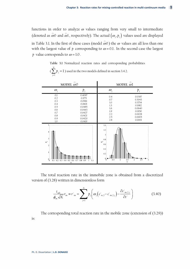
Chapter 3: Reaction rates for mixing‐controlled reaction in multi‐continuum media | 71
Ph. D. Dissertation | L.D. DONADO
functions in order to analyze values ranging from very small to intermediate
(denoted as
0 and
1 , respectively). The actual ,j jp values used are displayed
in Table 3.1. In the first of these cases (model
0 ) the values are all less than one with the largest value of p corresponding to 0.1 . In the second case the largest
p value corresponds to 1.0 .
Table 3.1 Normalized reaction rates and corresponding probabilities
(1
1N
jj
p
) used in the two models defined in section 3.4.2.
MODEL
0 MODEL
1
j jp j jp
0.1 0.2 0.3 0.4 0.5 0.6 0.7 0.8 0.9 1.0
0.4097 0.1771 0.0916 0.0601 0.0485 0.0443 0.0427 0.0421 0.0420 0.0419
0.4 0.7 1.0 1.3 1.6 1.9 2.2 2.5 2.8
0.0397 0.3043 0.3754 0.1982 0.0640 0.0150 0.0028 0.0005 0.0001
The total reaction rate in the immobile zone is obtained from a discretized version of (3.28) written in dimensionless form
,2,,2 ,2,
1
'' ' '
'
N
im jadvim im j j m im j
imj
ctr r p c c
tK
(3.40)
The corresponding total reaction rate in the mobile zone (extension of (3.29)) is:
72 | On multicomponent reactive transport in porous media: From the natural complexity to analytical solutions
Hydrogeology Group – GHS | UPC
22,22
mixing
,2,,20
1 1
mass transfer
'1 ''
' '
'''' * ' '
'
madv mm m
mm
N N
im jmm m j j im
mj j
ct ur r
Pe u xK
ccgg u u p p r
t u t
(3.41)
where the memory function is 1
j
N
Tj j
j
g T p e
.
In (3.32) we have separated the contributions from the mixing part (i.e., the
corresponding reaction if is taken equal to zero) from that of the heterogeneous
domain (i.e., the contribution of the memory function plus reactions in the immobile zone in our MRMT model).
The specific chemical problem considered is precipitation of siderite
( 2+ 2-3 3FeCO =Fe +CO ) with an equilibrium constant log 25º 10.7K C
[Coudrainribstein and Morel, 1987]. The porosity ratio was fixed at a constant value of
5/7, following the indications of Sanchez-Vila and Carrera [2004]. The reaction rate is
computed by the inverse Laplace transform of (3.37) using the de Hoog algorithm
[Hollenbeck, 1998]. Results are discussed in the next section.
3.5 Evaluation of the reaction rates
The dimensionless mass transfer rate ( ) represents the ratio between mass transfer rate and advection rate. It has a strong influence on the behavior of breakthrough curves (BTCs) of the dimensionless immobile concentration. In the
0 model, mass transfer is very slow. Correspondingly, solute transfers back to the
mobile zone with difficulty, causing significant tailing in BTC's. In the
1 model the characteristic times of mass transfer and dispersion are similar. Finally it should be
noted that if all values were very large (i.e., mass transfer between the mobile and immobile phases is instantaneous), the system would respond as that of a homogeneous media with a retardation factor equal to 1 , and consequently
reactions could be obtained from the results of De Simoni et al., [2005].
We start by looking at the reactive transport problem presented in the previous section in terms of normalized concentrations. Due to the particular choice of boundary conditions (step-input function), the initial water will eventually be
Chapter 3: Reaction rates for mixing‐controlled reaction in multi‐continuum media | 73
Ph. D. Dissertation | L.D. DONADO
substituted by the input water. This effect takes place faster in the mobile phase and eventually transmits to the different immobile phases (according to the corresponding values). In Figure 3.1 we see the evolution of the concentrations of
the components with time for two particular values of Pe (= 0.1, i.e., diffusion-
dominated problem or 10, i.e., advection-dominated problem) and for three different
distances ( 0.1, 1 10x and ). Unless stated otherwise, all figures include only the
results corresponding to model
0 . In the figure we observe a clear separation between the curves corresponding to the mobile and the immobile zones (the latter is actually the weighted arithmetic average of the component concentrations). For
the diffusive case (smaller Péclet number) the changes in the mobile zone occur earlier, which is a reflection of the diffusive front that propagates through the system. For completeness, Figure 3.2 displays the corresponding concentration of aqueous species obtained from the normalized expressions of the actual concentrations (3.27).
The distribution of reaction rates in space and time is presented next. Figure 3.3 displays the various contributions to the total reaction rates over time at three points in space. For the point closest to the inlet the mixing driven contribution (see equation (3.41)) is largest and it is only at late times that the mass transfer contribution dominates and becomes the main contributor to the total reaction rate. For large travel distances almost all of the reaction is driven by the mass transfer
term. While this holds true for both Péclet numbers, it is clearly visible that the mass
transfer term is more important in the higher Péclet number case. At short times, the concentration gradients are large and the reactions are driven by mixing due to local dispersion. With increasing time, gradients are smoothed out and mass transfer dominates over local dispersion as a mixing mechanism and becomes the dominating driving force of chemical reaction. This effect is more pronounced for advection-dominated transport ( Pe = 10). After the smoothing out of the large initial gradients, local dispersion plays only a subordinate role.
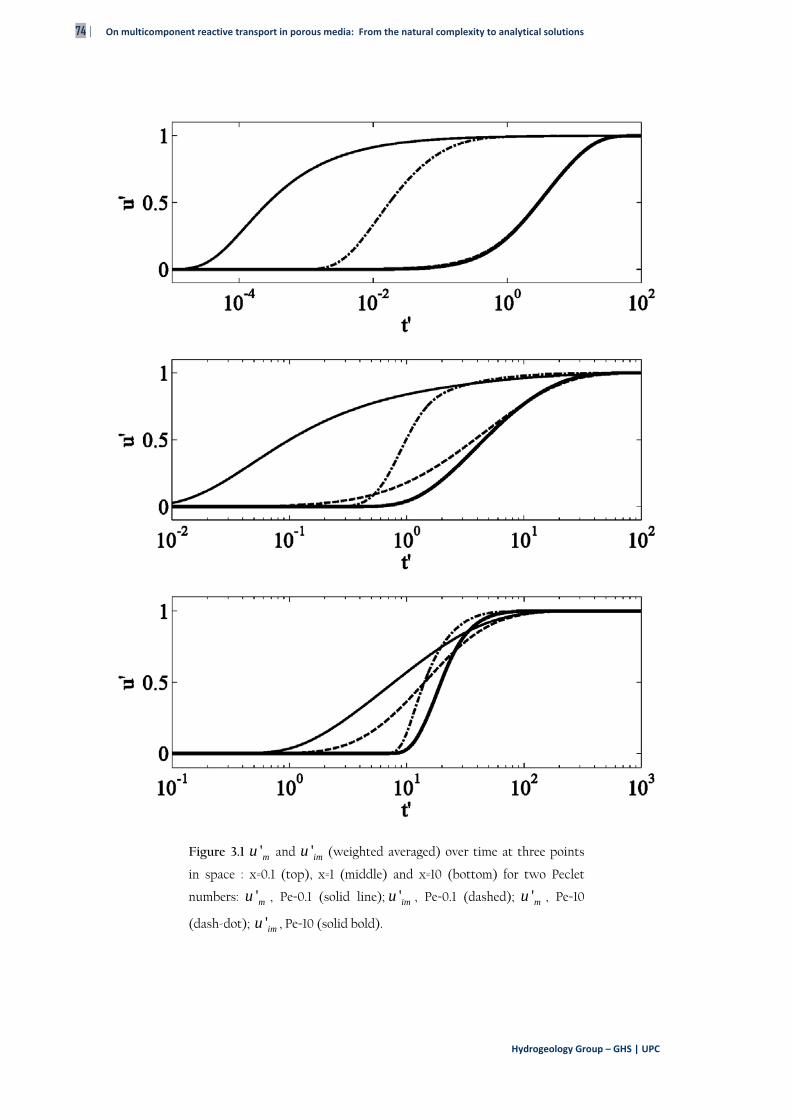
74 | On multicomponent reactive transport in porous media: From the natural complexity to analytical solutions
Hydrogeology Group – GHS | UPC
Figure 3.1 'mu and 'imu (weighted averaged) over time at three points
in space : x=0.1 (top), x=1 (middle) and x=10 (bottom) for two Peclet
numbers: 'mu , Pe=0.1 (solid line); 'imu , Pe=0.1 (dashed); 'mu , Pe=10
(dash-dot); 'imu , Pe=10 (solid bold).
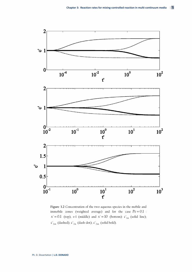
Chapter 3: Reaction rates for mixing‐controlled reaction in multi‐continuum media | 75
Ph. D. Dissertation | L.D. DONADO
Figure 3.2 Concentration of the two aqueous species in the mobile and
immobile zones (weighted average) and for the case 0.1Pe :
' 0.1 x (top), x=1 (middle) and ' 10 x (bottom): 1' mc (solid line);
1' imc (dashed); 2' mc (dash-dot); 2' imc (solid bold).
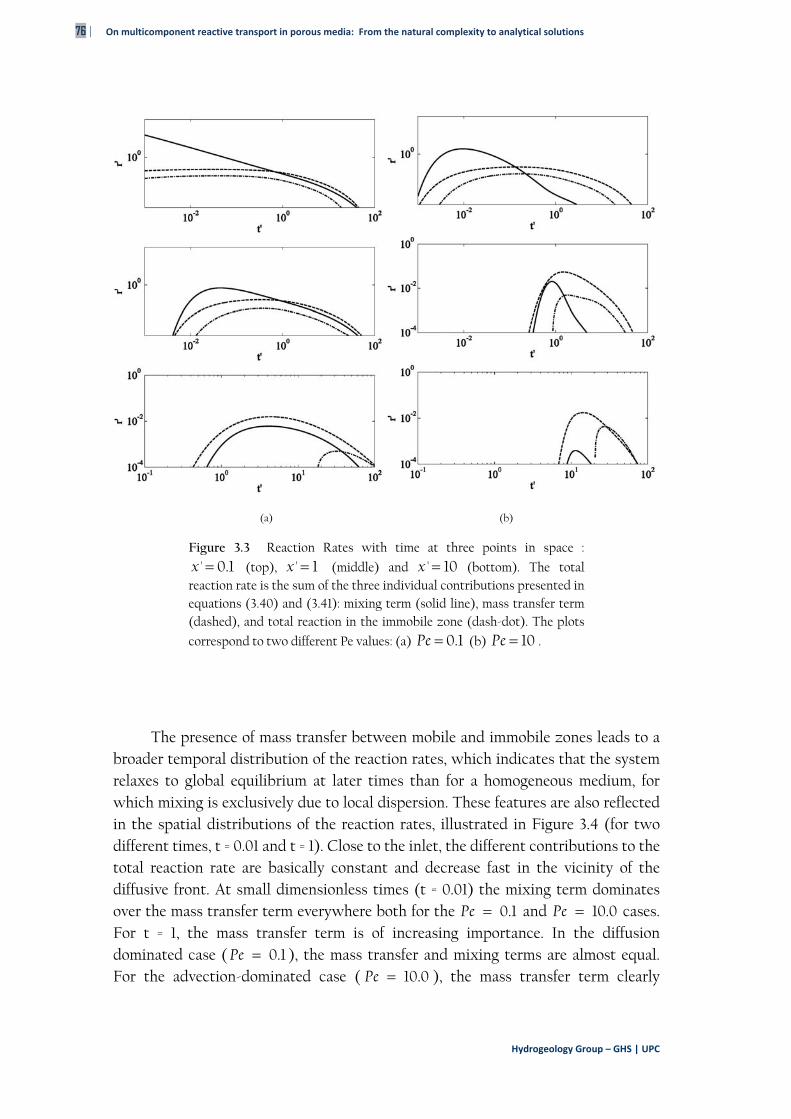
76 | On multicomponent reactive transport in porous media: From the natural complexity to analytical solutions
Hydrogeology Group – GHS | UPC
(a) (b)
Figure 3.3 Reaction Rates with time at three points in space :
' 0.1 x (top), ' 1 x (middle) and ' 10x (bottom). The total reaction rate is the sum of the three individual contributions presented in equations (3.40) and (3.41): mixing term (solid line), mass transfer term (dashed), and total reaction in the immobile zone (dash-dot). The plots
correspond to two different Pe values: (a) 0.1Pe (b) 10Pe .
The presence of mass transfer between mobile and immobile zones leads to a broader temporal distribution of the reaction rates, which indicates that the system relaxes to global equilibrium at later times than for a homogeneous medium, for which mixing is exclusively due to local dispersion. These features are also reflected in the spatial distributions of the reaction rates, illustrated in Figure 3.4 (for two different times, t = 0.01 and t = 1). Close to the inlet, the different contributions to the total reaction rate are basically constant and decrease fast in the vicinity of the diffusive front. At small dimensionless times (t = 0.01) the mixing term dominates over the mass transfer term everywhere both for the 0.1Pe and 10.0Pe cases. For t = 1, the mass transfer term is of increasing importance. In the diffusion dominated case ( 0.1Pe ), the mass transfer and mixing terms are almost equal. For the advection-dominated case ( 10.0Pe ), the mass transfer term clearly
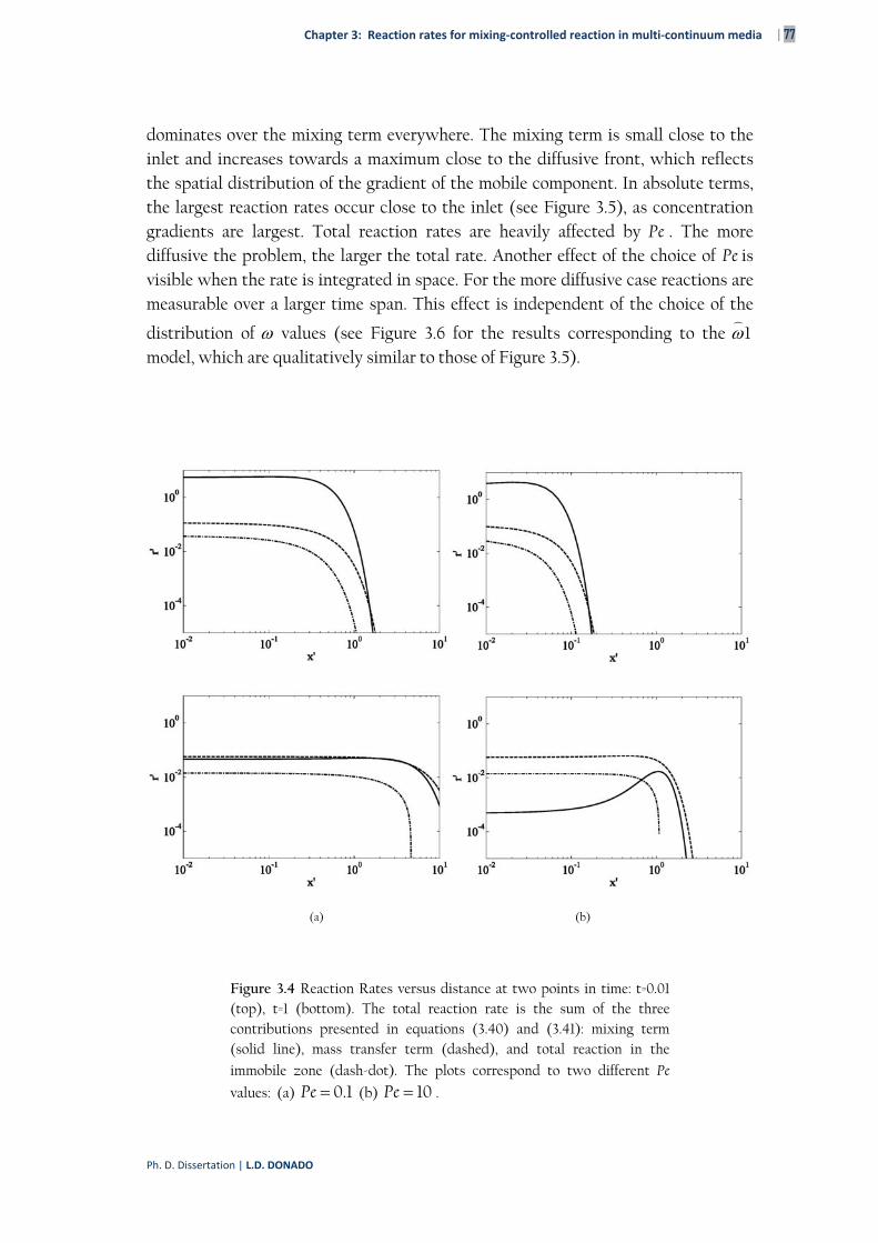
Chapter 3: Reaction rates for mixing‐controlled reaction in multi‐continuum media | 77
Ph. D. Dissertation | L.D. DONADO
dominates over the mixing term everywhere. The mixing term is small close to the inlet and increases towards a maximum close to the diffusive front, which reflects the spatial distribution of the gradient of the mobile component. In absolute terms, the largest reaction rates occur close to the inlet (see Figure 3.5), as concentration gradients are largest. Total reaction rates are heavily affected by Pe . The more diffusive the problem, the larger the total rate. Another effect of the choice of Pe is visible when the rate is integrated in space. For the more diffusive case reactions are measurable over a larger time span. This effect is independent of the choice of the
distribution of values (see Figure 3.6 for the results corresponding to the
1 model, which are qualitatively similar to those of Figure 3.5).
(a) (b)
Figure 3.4 Reaction Rates versus distance at two points in time: t=0.01 (top), t=1 (bottom). The total reaction rate is the sum of the three contributions presented in equations (3.40) and (3.41): mixing term (solid line), mass transfer term (dashed), and total reaction in the
immobile zone (dash-dot). The plots correspond to two different Pe
values: (a) 0.1Pe (b) 10Pe .
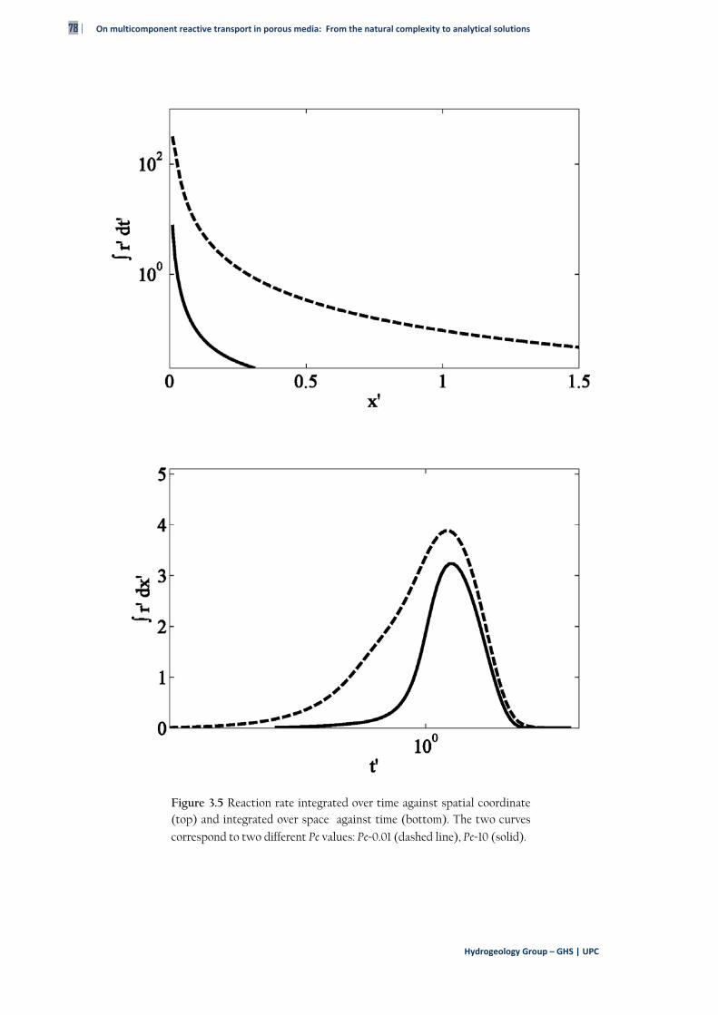
78 | On multicomponent reactive transport in porous media: From the natural complexity to analytical solutions
Hydrogeology Group – GHS | UPC
Figure 3.5 Reaction rate integrated over time against spatial coordinate (top) and integrated over space against time (bottom). The two curves
correspond to two different Pe values: Pe=0.01 (dashed line), Pe=10 (solid).
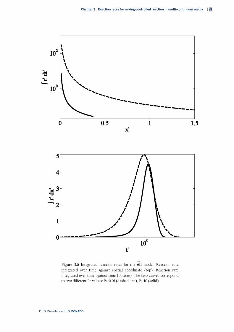
Chapter 3: Reaction rates for mixing‐controlled reaction in multi‐continuum media | 79
Ph. D. Dissertation | L.D. DONADO
Figure 3.6 Integrated reaction rates for the
1 model. Reaction rate integrated over time against spatial coordinate (top). Reaction rate integrated over time against time (bottom). The two curves correspond to two different Pe values: Pe=0.01 (dashed line), Pe=10 (solid).
80 | On multicomponent reactive transport in porous media: From the natural complexity to analytical solutions
Hydrogeology Group – GHS | UPC
3.6 Conclusions
We study mixing-driven reactive transport in an effective medium that is characterized by a mobile region and a suite of immobile regions which are characterized by a distribution of solute retention times. The mobile and immobile regions communicate by linear kinetic mass transfer. The retention properties are
the same at each point in space, i.e., the solute can encounter the full spectrum of retention zones at any point. Such an effective medium can be visualized as consisting of multiple overlapping continua. The resulting transport model is termed multi rate mass transfer (MRMT) model, providing an effective description of transport in heterogeneous media. In this approach, the medium heterogeneity is represented by the distribution of solute retention times.
By setting the geochemical problem in term of chemical components, we derive explicit expressions for the reaction rates in either the mobile and the immobile zones. We identify three contributions to the total reaction rate, (i) a term that is
identical in form to the one derived by De Simoni et al. [2005], which quantifies local dispersive mixing in the mobile region, (ii) a term that quantifies mixing due to mass transfer between the mobile and immobile regions, and (iii) a term that quantifies the total reaction in the immobile regions. The latter term is relatively small compared with the contributions from the mobile region. Nevertheless, the mass exchange between the mobile and immobile zones has an important effect on the reaction dynamics.
For advective-dispersive transport in a homogeneous medium, the only mixing mechanism is local dispersion, which induces non-equilibrium. In the presence of immobile regions, advective transport and mass transfer between the mobile and immobile zones leads to mixing of the mobile water and water that has been released from the immobile regions. This induces non-equilibrium and thus reaction. For local dispersive mixing, the typical mixing time scale is given by the dispersion time over the variation distance of the component distribution, while for mass transfer induced mixing, the time scale is given by the typical retention time scale, which can be very large. Thus, for reactive transport in a medium characterized by a broad distribution of retention times, the time for the system to reach global equilibrium can be significantly increased. Such mechanisms can not be captured by a macro-dispersion model, which would lead to an underestimation of the total reaction taking place.
Heterogeneity is accounted by means of an effective dynamics approach, where the system is homogeneized by means of a multi-rate mass transfer approach. The mobile zone accounts for the fastest paths, while the less mobile zones are assumed as immobile, interexchanging mass with the mobile zone by means of a
Chapter 3: Reaction rates for mixing‐controlled reaction in multi‐continuum media | 81
Ph. D. Dissertation | L.D. DONADO
prespecified distribution of constant rates. This model has extensively be used in the literature to account for transport of conservative species. An important result of this work is an analytical solution of the reaction rate term for multicomponent systems was derived. Our first conclusion is that when we account for mixing driven reactions, the choice of the degree of heterogeneity, as well as the mass transfer rates has a definite quantitative impact.
Heterogeneous reaction rate is directly proportional to total capacity factor, which in our model is a measure of the degree of heterogeneity of the system. It is also important to note that since reactions are driven by mixing, which is itself driven by local dispersion/diffusion, in advective dominated cases the total reaction taking place in the mobile phase is quite small, but this is not the case for the reactions taking place in the immobile zone. As a consequence, in advective dominated systems, the main contribution for the reaction rates is due to explicitly acknowledging heterogeneity. Homogenizing the system by means of upscaling
parameters (i.e., a macrodispersive approach) would lead to a clear underestimation of the total reaction taking place in the system.

(This page intentionally left blank.)
chapter
On multicomponent reactive transport in porous media: From the natural complexity to analytical solutions

(This page intentionally left blank.)
Chapter 4: Transport‐controlled reaction rates under local non‐equilibrium conditions | 81
Ph. D. Dissertation | L.D. DONADO
Chapter 4
Transport‐controlled reaction rates under local non‐equilibrium conditions
4 TRANSPORT‐CONTROLLED REACTION
RATES UNDER LOCAL NON‐EQUILIBRIUM
CONDITIONSHOMOGENEOUS MEDIA
4.1 Introduction
Chemical reactions in aquatic systems are driven by non-equilibrium conditions. When at a given point the concentrations of the reacting species do not satisfy the law of mass action, the system reacts by changing these concentrations, driving the system towards equilibrium. In reactive transport problems, reactions are driven by (1) local non-equilibrium due to deviations of the locally uniform species concentrations from the law of mass action and (2) global non-equilibrium due to transport-controlled mixing, which leads to spatial variations in the aqueous species concentrations.
Solute transport and mixing are governed by advection, diffusion and hydrodynamic dispersion. These processes are linear in the species concentrations. Chemical interactions induce non-linearities, since the reaction rates, incorporated
82 | On multicomponent reactive transport in porous media: From the natural complexity to analytical solutions
Hydrogeology Group GHS | UPC
as sink/source terms in the global mass balances, are non-linear in the species concentrations. The local scale reaction rates are modeled by inferring the dynamics determined in a well-mixed reactor while assuming complete mixing of the species locally.
The chemical evolution of a multispecies system can be fully described in terms of reaction rates. In a well stirred environment (complete mixing assumed), the reaction rate is homogeneous in space due to the uniform species concentrations, and solely varies in time. Its temporal evolution reflects the reaction dynamics and describes the relaxation of the system towards equilibrium. In a reactive transport problem, reaction rates are a function of space and time because the species concentrations vary spatio-temporally. The reaction rate provides a map of where reactions occur in the medium. As such, reaction rates contain valuable information about the transport-controlled global reaction dynamics. Thus, in order to properly address and understand the dynamics of multicomponent reactive transport, it is necessary to have a methodology at hand to compute the reaction rates at any location in space and time.
Because of its mathematical complexity, the solution of multicomponent reactive transport problems in general, and the computation of reaction rates in particular, have been mostly tackled using numerical approaches. A few studies deal with analytical solutions to simplified reactive transport problems, such as
homogeneous bimolecular reactions [Ham et al., 2004], biodegradation in natural
attenuation problems [Liedl et al., 2005; Cirpka et al., 2006], and heterogeneous or
homogeneous reactions involving multiple aqueous species and minerals [De Simoni et
al., 2005; 2007]. In all these cases the geochemical problems are characterized by
local instantaneous equilibrium. Kechagia et al. [2002] studied the upscaling of fast chemical reactions from the pore to the Darcy scale using volume-averaging techniques and discuss the validity of the continuum approach for fast local scale reactions.
Local scale equilibrium can be assumed to hold if the reaction time r is small
compared to a typical dispersion time scale D . The dispersion scale is compared to
the reaction time scale r by the non-dimensional Damköhler number Da , defined
as [e.g., Knapp, 1989],
D
r
Da (4.1)
Note that dispersion is the relevant mass transfer mechanism in the context of the mixing-limited reactions under consideration here. Advective transport has the effect of a mere translation of a fluid element in space.
Chapter 4: Transport‐controlled reaction rates under local non‐equilibrium conditions | 83
Ph. D. Dissertation | L.D. DONADO
Under the assumption of an instantaneous local chemical reaction, i.e., Da ,
[De Simoni et al., 2005] presented a methodology for the derivation of the spatiotemporal distribution of the reaction rate. The resulting expression is the product of two terms: (1) a mixing controlled contribution, which depends on the local dispersion tensor; and (2) a speciation term, containing the details of the local chemical reaction.
For local non-equilibrium conditions (i.e. finite Damköhler numbers), the species concentrations cannot be decoupled from the reaction rates, complicating the mathematical problem. So, it is not possible to derive an explicit expression for the reaction rate.
Figure 4.1 illustrates the problem for a simple geochemical system involving precipitation of a mineral caused by the reaction of two aqueous species. In the case of instantaneous equilibrium, only the configurations along the line corresponding to the law of mass action (a hyperbola in Figure 4.1) are valid configurations. If at some point two waters with different chemical signatures (still both in perfect chemical equilibrium with the mineral) mix and no reaction takes place, the concentrations would be along the dashed line, leading for example to point A (oversaturated with respect to the mineral). Instantaneous reaction would take the concentrations to point B . Instead, if equilibrium is non-instantaneous, any point in the 1 2c c space is a valid configuration. If water 1W mixes with water 2W , and if
diffusion is very fast compared to reaction (small Da ) the path would be 1W A B B , along straight lines. Any point along the line is valid, and so it is
possible that water in point B mixes with additional 2W water; the resulting mixtures would be now along the new dashed line. If, instead, reaction is fast, then the path would be 1W B , but now along the hyperbola. In such a case, the chemical evolution is a succession of equilibrium states.
The assumption of instantaneous equilibrium reduces the dimensionality of the problem through the law of mass action. Thus, non-instantaneous reactions lead to a more complex problem in mathematical terms. Reactions and concentrations cannot be decoupled, and no explicit expressions might be obtained. Instead it is possible to derive a non-linear evolution equation for the distribution of reaction rates. For fast local-scale reactions (large Da ), we derive a perturbation series of the reaction rate in powers of the inverse Damköhler number. In first order, we obtain an explicit expression for the reaction rate. The zeroth-order contribution recovers
the solution for local instantaneous equilibrium by [De Simoni et al., 2005].
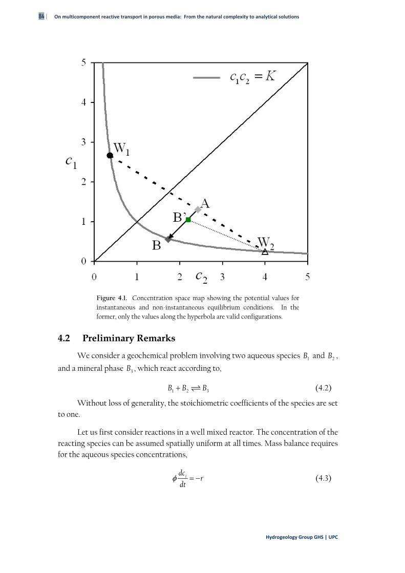
84 | On multicomponent reactive transport in porous media: From the natural complexity to analytical solutions
Hydrogeology Group GHS | UPC
Figure 4.1. Concentration space map showing the potential values for instantaneous and non-instantaneous equilibrium conditions. In the former, only the values along the hyperbola are valid configurations.
4.2 Preliminary Remarks
We consider a geochemical problem involving two aqueous species 1B and 2B ,
and a mineral phase 3B , which react according to,
1 2 3B B B (4.2)
Without loss of generality, the stoichiometric coefficients of the species are set to one.
Let us first consider reactions in a well mixed reactor. The concentration of the reacting species can be assumed spatially uniform at all times. Mass balance requires for the aqueous species concentrations,
idcr
dt (4.3)
Chapter 4: Transport‐controlled reaction rates under local non‐equilibrium conditions | 85
Ph. D. Dissertation | L.D. DONADO
with i = 1, 2; porosity is denoted by . The concentrations of the aqueous species (in
molar mass per unit volume of fluid) are denoted by 1c and 2c . Here, the species
concentrations depend only on time. For the reaction rate r ( 0r indicating precipitation), we employ the model given by, e.g., Knapp [1989], Steefel and Lasaga [1994], Lasaga et al. [1994], and Langmuir [1997],
0 1r Sk (4.4)
where the effective reaction time r is defined by
0
r
KSk
(4.5)
with 0k the rate constant, S the specific reactive surface, and K the local
equilibrium constant. Finally, is the ion activity product, given by 1 2 /c c K .
The conservative component [e.g., Lichtner, 1985],
1 2u c c (4.6)
decouples the nonlinear system of equations (4.3). As / 0du dt , the
conservative component 0 00 1 2
t tu u c c is constant. Thus, (4.3) can be solved
straightforwardly for the species concentrations by separation of variables. This yields for the reaction rate the explicit expression,
2 2
20 01 41 1 tanh
4 2r r
u K u tr K A
K K
(4.7)
with the constant A given by the initial conditions,
1 0 0 21 2 0tanh / 4t tA c c u K . In the limiting case of rt , r tends to zero and
the system equilibrates. The statement 1 2c c K (law of mass action) is, thus,
equivalent to 0r . For transport-controlled reactions these two statements are not equivalent. We will address this point later.
4.3 Transport-Controlled Reaction
Mass conservation implies that the concentrations ,ic tx of the aqueous
species ( 1,2i ) are governed by the following transport equations,
ii i
cc c r
t
q D (4.8)
86 | On multicomponent reactive transport in porous media: From the natural complexity to analytical solutions
Hydrogeology Group GHS | UPC
The specific discharge is denoted by q , and D denotes the bulk dispersion
tensor. Without loss of generality we set 1 in the following. The reaction rate r is
given by (4.4), which implicitly assumes that the reacting species are well mixed and their concentrations are uniform on a local support volume iV characterized by
the length scale l . Note that the validity of the continuum approach for very fast local scale reactions is in fact subject of discussion. Here, we assume the existence of a local support scale and leave this important question aside. Kechagia et al.[2002] addressed this issue in their paper on the upscaling of reactive transport processes from the pore to the Darcy scale.
We distinguish here two typical transport time scales; the advection time
scale /a l q , and the dispersion time scale 2 /D l D with D a characteristic
dispersion measure (here, for simplicity, we characterize the effect of dispersion by a single time scale, while in general there could be more than one involving the directional dispersion coefficients). The Péclet number /D aPe quantifies the
relative importance of dispersive and advective transport mechanisms. Note that the dispersion scale is the reaction limiting mass transfer mechanism. In the absence of dispersion, no reaction takes place since waters in contact do not mix and are just advected.
We non-dimensionalize (4.8) by rescaling the spatial coordinates by l ( /i ix x l ), time by the dispersion time scale D ( / Dt t ), and concentrations by
K ( /i ic c K ). This yields
ii i
cc c r
t
q D (4.9)
with the re-scaled reaction rate written in terms of the Damköhler number defined in (4.1)
1r Da (4.10)
The dimensionless discharge and dispersion tensor are defined by /D l q q
and 2/D l D D ; denotes the nabla operator in the dimensionless coordinates.
For compactness of notation, in the following the primes are omitted.
The independent component (4.6) is conservative and evolves according to,
0u
u ut
q D (4.11)
From equations (4.6) and (4.10) we obtain explicit expressions for 1c and 2c ,
Chapter 4: Transport‐controlled reaction rates under local non‐equilibrium conditions | 87
Ph. D. Dissertation | L.D. DONADO
21 / 2
14 1
2 2u
c u (4.12)
where we defined r , being the inverse Damköhler number ( 1Da ).
According to (4.12), the ic are only functions of the independent components u and
(i.e., ,i ic c u ). Thus, applying the chain rule to (4.9), and after some algebra,
we obtain the following non-linear partial differential equation for the dimensionless reaction rate r ,
2 2 2
22 2
2 T T Ti i i ir c c c cr r u r r r r u u
t u u
q D D D D (4.13)
It turns out that (4.13) does not depend on i , as can be easily seen by inserting (4.12) into (4.13); in the following we choose 2i .
The solution methodology can be detailed as follows. First, the linear equation (4.11) is solved for u , either numerically or, if possible, analytically. Then r remains the only unknown, and can be obtained by solving (4.13). Since this equation is non-linear in r , the solution must in general be sought numerically. In the case of large
Damköhler numbers, r can be expanded into a series in 1Da , from which an approximate solution for r can be obtained by truncation. This is explored in the next section.
4.4 Large Damköhler Numbers
For 1 ( 1Da ), the reactive transport system is close to local equilibrium at all points. De Simoni et al. [2005] derived an explicit exact expression for the
reaction rate in the case 0 , which is equivalent to the condition 1 2c c K , i.e., the
mass action law is fulfilled locally. Their result proves that the 00lim r r exists,
which implies that 1 for small values. Note that for the wellmixed
reactor, 1 2c c K implies 0r , while in a reactive transport scenario, even though
local equilibrium is reached instantaneously, the reaction rate remains finite as a consequence of transport-driven changes in the concentration values.
For large Da , we obtain an approximate solution for the reaction rate by means of an expansion into a series in powers of the inverse Damköhler number
0
nn
n
r r
(4.14)
88 | On multicomponent reactive transport in porous media: From the natural complexity to analytical solutions
Hydrogeology Group GHS | UPC
For bounded 0r , 1 for 1 . Thus, for small , the species
concentration 2c , can be expanded into a series in powers of 1r , which
gives,
2 2
0
n nn
n
c r r c
, 22
0
1!
nn
n
cc
n
(4.15)
Inserting (4.14) into (4.15), we obtain,
2 2
0 0
kn nk
k nk n
c R c
(4.16)
where nkR the are given by
1 2
1 1 2 2 1 1
1 2 10 0
nn n n
n
m mkn k m m m m m m
km m m
R r r r r
(4.17)
for 1n . In particular, for 0n , 0
0k kR and for 1n , 1 k
kR r .
Inserting (4.14) and (4.16) into (4.13) and collecting terms of the order k
yields a recursive relation for kr . Here we focus on the zeroth and first-order
contributions to r . The zeroth order term 0r is given by
02
0 22
Tcr u u
u
D (4.18)
The resulting expression for 0r is identical to the one derived by De Simoni et al.
[2005] under local instantaneous equilibrium conditions, i.e., in the limit of Da
(in this case 02 2c c ). For the first-order contribution 1r , we obtain,
0 1 12
1 0 0 1 0 02 22 2
2T Tr c cr r r c r u u u r
t u u
q D D D (4.19)
Note that equation (4.19) is explicit, since from (4.15), 02c and 1
2c are given by
explicit expressions,
0 22
14
2 2u
c u 12 2
1
4c
u
(4.20)
With this same methodology it would also be possible to obtain explicit
expressions for higher order terms ir , 1i .
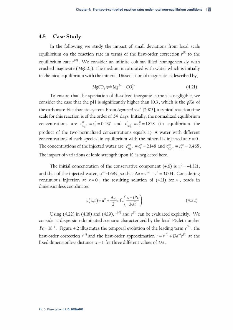
Chapter 4: Transport‐controlled reaction rates under local non‐equilibrium conditions | 89
Ph. D. Dissertation | L.D. DONADO
4.5 Case Study
In the following we study the impact of small deviations from local scale
equilibrium on the reaction rate in terms of the first-order correction 1r to the
equilibrium rate 0r . We consider an infinite column filled homogeneously with crushed magnesite ( 30MgC ). The medium is saturated with water which is initially
in chemical equilibrium with the mineral. Dissociation of magnesite is described by,
2 23 3MgCO Mg CO (4.21)
To ensure that the speciation of dissolved inorganic carbon is negligible, we consider the case that the pH is significantly higher than 10.3 , which is the pKa of
the carbonate-bicarbonate system. From Azaroual et al. [2003], a typical reaction time scale for this reaction is of the order of 54 days. Initially, the normalized equilibrium
concentrations are 20 0
1 0.537Mg
c c and 23
0 02 1.858
COc c (in equilibrium the
product of the two normalized concentrations equals 1 ). A water with different concentrations of each species, in equilibrium with the mineral is injected at 0x .
The concentrations of the injected water are, 201 2.148ext
Mgc c and 2
32 0.465ext ext
COc c .
The impact of variations of ionic strength upon K is neglected here.
The initial concentration of the conservative component (4.6) is 0 1.321u ,
and that of the injected water, extu =1.683 , so that 0 3.004extu u u . Considering continuous injection at 0x , the resulting solution of (4.11) for u , reads in dimensionless coordinates
0, erfc2 2
u x tPeu x t u
t
(4.22)
Using (4.22) in (4.18) and (4.19), 0r and 1r can be evaluated explicitly. We consider a dispersion-dominated scenario characterized by the local Péclet number
110Pe . Figure 4.2 illustrates the temporal evolution of the leading term 0r , the
first-order correction 1r and the first-order approximation 0 11r r Da r at the fixed dimensionless distance 1x for three different values of Da .
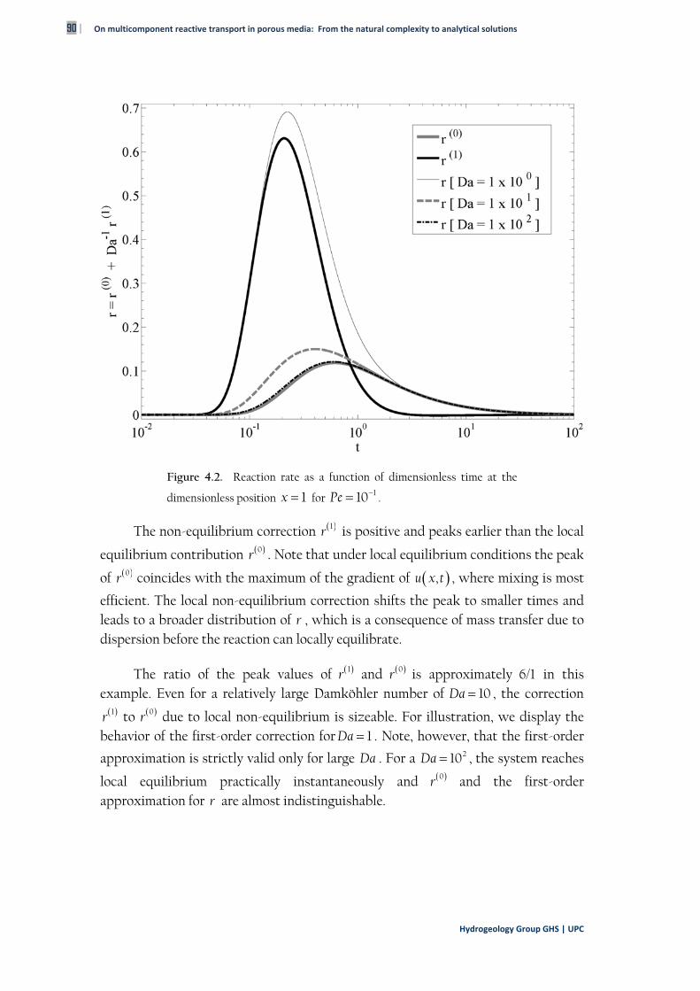
90 | On multicomponent reactive transport in porous media: From the natural complexity to analytical solutions
Hydrogeology Group GHS | UPC
Figure 4.2. Reaction rate as a function of dimensionless time at the
dimensionless position 1x for 110Pe .
The non-equilibrium correction 1r is positive and peaks earlier than the local
equilibrium contribution 0r . Note that under local equilibrium conditions the peak
of 0r coincides with the maximum of the gradient of ,u x t , where mixing is most
efficient. The local non-equilibrium correction shifts the peak to smaller times and leads to a broader distribution of r , which is a consequence of mass transfer due to dispersion before the reaction can locally equilibrate.
The ratio of the peak values of 1r and 0r is approximately 6/1 in this example. Even for a relatively large Damköhler number of 10Da , the correction 1r to 0r due to local non-equilibrium is sizeable. For illustration, we display the
behavior of the first-order correction for 1Da . Note, however, that the first-order
approximation is strictly valid only for large Da . For a 210Da , the system reaches
local equilibrium practically instantaneously and 0r and the first-order approximation for r are almost indistinguishable.
Chapter 4: Transport‐controlled reaction rates under local non‐equilibrium conditions | 91
Ph. D. Dissertation | L.D. DONADO
Figure 4.3. Reaction rate as a function of normalized distance at
dimensionless time 0.5t for 110Pe .
Figure 4.3 shows a snapshot of 0r , 1r and the first-order approximation versus distance at a fixed time, again for three different Damköhler numbers. The
behavior of 0r is basically determined by the gradient of the conservative component, see (4.18), and assumes a maximum where the gradient of u is maximal. The first-order correction shows a very different behavior with two positive peaks and a negative one in between. The peak of the resulting first-order correction is shifted in the positive x -direction as a result of advection. Mass transfer due to
dispersion, again, leads to a broader spatial distribution for r rather than for 0r . For a value of 1Da , the shape of the first-order approximation is very different from
the one of 0r . It has forward and backward peaks, while in between it can assume negative values, indicating dissolution. However, as mentioned above, the first-
order approximation is strictly valid only for large Da . Again, for 100Da , 0r and the first-order approximation for r are practically indistinguishable.
4.6 Discussion
We present an analytical approach to study reactive transport under local non-equilibrium conditions. The reaction rate can be used as the main variable
92 | On multicomponent reactive transport in porous media: From the natural complexity to analytical solutions
Hydrogeology Group GHS | UPC
characterizing the multispecies transport system. For instantaneously reached chemical equilibrium the reaction rate can be evaluated explicitly in terms of components (linear combinations of the species concentrations behaving conservatively). Under local-scale non-equilibrium conditions the reaction rate can be obtained as the solution of a non-linear PDE and depends on the ratio between the characteristic dispersion and reaction times.
We use an expansion of the reaction rate for large Damköhler numbers to analyze the system behavior for small deviations from local equilibrium. Even small deviations from local equilibrium can have a sizeable impact on the shape and magnitude of the reaction rate distribution in space, increasing its width and changing the peak position compared to the behavior under local equilibrium conditions. The impact of larger deviations from local equilibrium (typical mass transfer time smaller than the reaction time scale) needs to be analyzed by a full (numerical) solution of the non-linear partial differential equation (13) and comparison to experiments and direct numerical simulations.
chapter
On multicomponent reactive transport in porous media: From the natural complexity to analytical solutions

(This page intentionally left blank.)
Chapter 5: Simultaneous Equilibrium and Kinetic reaction rates | 93
Ph. D. Dissertation | L.D. DONADO
Chapter 5
Simultaneous Equilibrium and Kinetic reaction rates
5 SIMULTANEOUS EQUILIBRIUM AND KINETIC
REACTION RATES
5.1 Introduction
Chemical reactions may affect the fate of pollutants and the properties of the host porous medium. However, the conditions for the reactions to occur, their
location, and often their rate, are largely controlled by transport [Rezaei et al., 2005], which is what motivates analyses of reactive transport. Modeling multicomponent reactive transport problems requires specifying (a) a set of mass balance equations, one for each species being transported, and (b) a second set of equations describing the reactions amongst species. Mass balance of each individual species is expressed by a solute transport equation with a source term to account for all the reactions participated by each individual species. The transport equation itself can be written according to different conceptual models. These include the advection dispersion
equation (ADE) [e.g., Bear, 1972], dual- or multiple-domain mass transfer models
[e.g., Haggerty and Gorelick, 1995; Carrera et al., 1998; Cvetkovic et al., 1999; Berkowitz et al.,
2008], fractional derivatives [e.g., Benson et al., 2000a; Cushman and Ginn, 2000], or
continuous time random walks [e.g., Berkowitz and Scher, 1995; Berkowitz et al., 2006].
94 | On multicomponent reactive transport in porous media: From the natural complexity to analytical solutions
Hydrogeology Group – GHS | UPC
From a pragmatic standpoint, chemical reactions can be subdivided into two
broad groups, i.e., “sufficiently fast” and “insufficiently fast” reactions [Rubin, 1983], depending on whether a characteristic reaction time is much smaller than the time
scales associated with other mass-transfer processes (e.g., advection, diffusion, dispersion). In the presence of “sufficiently fast” reactions the assumption of local chemical equilibrium can be considered appropriate. This is the case for most aqueous reactions. On the other hand, reactions involving minerals and aqueous
species are often better described as kinetic, that is, “insufficiently fast” [e.g., Steefel
and Lasaga, 1994]. Whenever reactions with different characteristic times occur simultaneously, the solution of the associated multicomponent system becomes
mathematically complex due to the presence of non-linearities [e.g., Steefel and Lasaga,
1994; Steefel and MacQuarrie, 1996; Molins et al., 2004; Steefel et al., 2005 and references therein].
A crucial element in the analysis of reactive transport scenarios is the assessment of the space-time patterns of reaction rates. This allows: (1) identifying the position and magnitude of the maximum local rates, which may have significant impacts on hydraulic properties, including formation of wormholes in dissolution problems, or occurrence of clogging and diagenetic phenomena in precipitation or
biological problems [e.g., Kielland, 1937; Steefel and MacQuarrie, 1996; Krautle and
Knabner, 2005], (2) identifying the extent of the domain contributing to the observed process, and (3) providing information about the rate of evolution of the system towards equilibrium conditions.
A series of mathematical formulations to solve multicomponent reactive transport problems are available in the literature, and included in a variety of codes
[e.g., Rubin, 1990; Kinzelbach et al., 1991; Yeh and Tripathi, 1991; Friedly and Rubin, 1992;
Rubin, 1992; Lichtner, 1996; Steefel and MacQuarrie, 1996; Clement et al., 1998; Saaltink et al.,
1998; Tebes-Stevens et al., 1998; Parkhurst and Appelo, 1999; Robinson et al., 2000; Saaltink et
al., 2001; Molins et al., 2004; Krautle and Knabner, 2005]. All these methodologies are based on the idea that reactive transport problems can be reformulated as follows: (a)
defining the chemical system in terms of components (i.e., linear combinations of reactive species concentrations); some of these components are conservative so that their associated transport equations can be decoupled from the full system, while other components (termed kinetic components) are associated with kinetic reactions and cannot be completely decoupled; (b) solving the transport equations for the conservative components; (c) calculating the kinetic components by solving a nonlinear algebraic system of equations; (d) performing speciation calculations to obtain the concentration of aqueous species from the space-time distribution of components; and (e) substituting the latter into the transport equations to evaluate
Chapter 5: Simultaneous Equilibrium and Kinetic reaction rates | 95
Ph. D. Dissertation | L.D. DONADO
numerically reaction rates. This approach can be applied when the concentrations of the reacting species stand in algebraic relationship to each other and transport
parameters are identical for all compounds (e.g., if an ADE were used, that would meant that all species are subject to the same advective velocity and diffusion/dispersion coefficients). The former requirement is met by systems either
in local chemical equilibrium or instantaneous, complete, irreversible reactions [e.g.,
Ham et al., 2004; Liedl et al., 2005] and can also be used for specific cases of kinetic
reactions [Molins et al., 2004; Cirpka and Valocchi, 2007].
A methodology to compute directly homogeneous and heterogeneous reaction
rates under instantaneous equilibrium has been presented by De Simoni et al. [2005; 2007]. Their general expression for the reaction rates illustrates that mixing
processes control equilibrium reaction rates. De Simoni et al. [2005; 2007] solve two independent problems: (a) the transport of one or more conservative species, and (b)
chemical speciation. The approach has been used by Guadagnini et al. [2009] in conjunction with laboratory-scale CaCO3 dissolution experiments reported in
Singurindy et al. [2004] to describe spatial distribution of equilibrium reactions rates in a homogeneous flow cell. Deconstructing the full reactive transport problem into two independent ones (transport of conservative species and speciation) has
additional advantages. For instance, Sanchez-Vila et al. [2009] employed it to obtain the probability density function of aqueous species concentrations in a randomly heterogeneous stratified medium.
Whenever reactions do not occur under equilibrium conditions it is not possible to evaluate explicitly reaction rates. Still, it is possible to pose the problem so that reaction rates are the dependent variables. In the case of a bi-molecular system where two aqueous species react to produce non-instantaneous
precipitation/dissolution of a mineral, Sanchez-Vila et al. [2007] found that reaction rates can be obtained by solving a non-linear partial differential equation. When the kinetic reaction is fast, the latter equation can be solved by means of a perturbation expansion in terms of the inverse of the Damköhler number, where the leading order
term corresponds to the expression already provided by De Simoni et al. [2005] for instantaneous equilibrium.
Here we develop an exact analytical expression for the reaction rates associated with a multicomponent reactive transport problem in the presence of both kinetic and equilibrium chemical reactions. Selecting whether a reaction can be considered instantaneous in a real geochemical problem is not a trivial task. When several reactions take place simultaneously, the reaction characteristic times, ,r i
( 1, ..., ; r ri N N being the number of reactions), span over several orders of
96 | On multicomponent reactive transport in porous media: From the natural complexity to analytical solutions
Hydrogeology Group – GHS | UPC
magnitude. In a given subsurface transport problem one is typically concerned with a range of times which can usually be related to some transport characteristic time,
t . All reactions characterized by ,r i t can be treated mathematically as
instantaneous. On the other hand, reactions associated with ,r i t can be typically
neglected. Thus, only reactions associated with characteristic times comparable to
t need to be treated as kinetically driven.
On the basis of this reasoning, we consider here a system where only one reaction is kinetically controlled, while allowing for any number of equilibrium reactions to take place simultaneously. The methodology could be extended to include the presence of more than one kinetic reaction. This would only contribute to increase the casuistic without any added benefit to the conceptual part of the work.
We start from the work of Molins et al. [2004] and De Simoni et al. [2005] and develop expressions for the space-time distribution of reaction rates for a two-reactions system, when only one reaction occurs under instantaneous equilibrium. The equilibrium reaction rate is expressed as a function of a mixing-related term, the distribution of (conservative and kinetic) components and the kinetic reaction rate. The resulting expressions are then solved numerically to simulate the dissolution of calcite in the presence of precipitating gypsum. We conclude by presenting the generalization of the formulation for a multicomponent system characterized by an arbitrary number of equilibrium reactions and one kinetic reaction.
5.2 Two Reaction Model
The general formulation for a system involving several equilibrium reactions will be presented in Section 5.4. Here, we discuss the solution for a particular two-reaction system, which facilitates presenting the general ideas and the benefits of the
methodology. The system involves the precipitation/dissolution of two minerals ( )4
sB
and ( )5
sB in the presence of three aqueous species, 1B , 2B , and 3B , one of them
participating in both reactions (common ion effect). The reactions considered are
( )1 2 4
sB B B , (5.1)
( )1 3 5
sB B B . (5.2)
We treat both mineral as pure phases so that their activity is unity. We consider (5.1) to occur at equilibrium at all points in the domain. On the contrary,
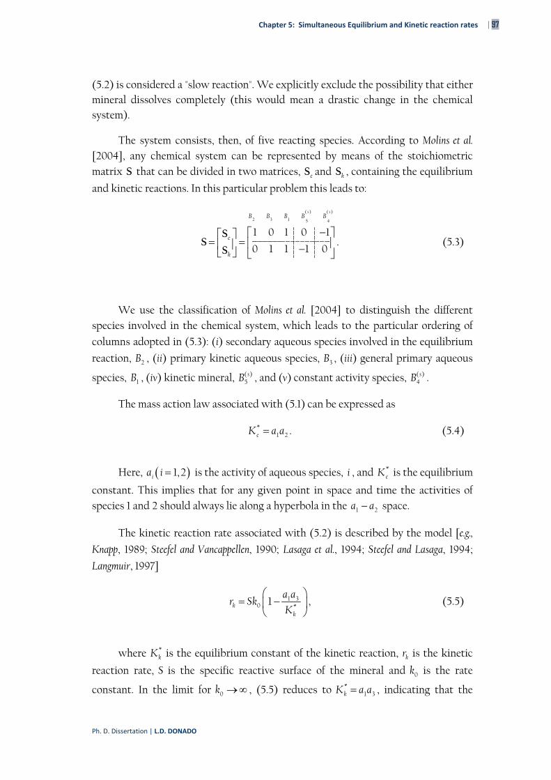
Chapter 5: Simultaneous Equilibrium and Kinetic reaction rates | 97
Ph. D. Dissertation | L.D. DONADO
(5.2) is considered a "slow reaction". We explicitly exclude the possibility that either mineral dissolves completely (this would mean a drastic change in the chemical system).
The system consists, then, of five reacting species. According to Molins et al. [2004], any chemical system can be represented by means of the stoichiometric matrix S that can be divided in two matrices, eS and kS , containing the equilibrium
and kinetic reactions. In this particular problem this leads to:
( ) ( )
2 3 1 5 4
1 0 1 0 1
0 1 1 1 0
s s
e
k
B B B B B
SS
S. (5.3)
We use the classification of Molins et al. [2004] to distinguish the different species involved in the chemical system, which leads to the particular ordering of
columns adopted in (5.3): (i) secondary aqueous species involved in the equilibrium
reaction, 2B , (ii) primary kinetic aqueous species, 3B , (iii) general primary aqueous
species, 1B , (iv) kinetic mineral, ( )5
sB , and (v) constant activity species, ( )4
sB .
The mass action law associated with (5.1) can be expressed as
*1 2eK a a . (5.4)
Here, 1,2ia i is the activity of aqueous species, i , and *eK is the equilibrium
constant. This implies that for any given point in space and time the activities of species 1 and 2 should always lie along a hyperbola in the 1 2a a space.
The kinetic reaction rate associated with (5.2) is described by the model [e.g.,
Knapp, 1989; Steefel and Vancappellen, 1990; Lasaga et al., 1994; Steefel and Lasaga, 1994;
Langmuir, 1997]
1 30 *
1kk
a ar Sk
K, (5.5)
where *kK is the equilibrium constant of the kinetic reaction, kr is the kinetic
reaction rate, S is the specific reactive surface of the mineral and 0k is the rate
constant. In the limit for 0k , (5.5) reduces to *1 3kK a a , indicating that the
98 | On multicomponent reactive transport in porous media: From the natural complexity to analytical solutions
Hydrogeology Group – GHS | UPC
reaction is in equilibrium for all practical purposes. Coefficients *eK and *
kK usually
depend on temperature and pressure. For simplicity, they will be assumed constant in this work.
Activities ( )ia and concentrations of aqueous species ( )ic are related by
ii
i
ac , (5.6)
where i is the activity coefficients for the i-th aqueous species. For moderately
saline solutions i can be approximated by the extended Debye-Hückel equation
2
0log1
ii
i
Az Ib I
a B I. (5.7)
Here A and B are temperature dependent parameters (for a temperature of
25 C , 0.5092A and 0.3282B ), b
= 0.041, and 0
ia is the ionic radius [Kielland,
1937] of species i; I is the ionic strength, defined as
2
1
12
sN
i ii
I c z , (5.8)
where jz is the valence of species j. Within the range of validity of (5.7), i
depends only, and weakly, on I, which typically does not vary much in space and time. This allows recasting the geochemical problem in terms of concentrations,
rather than activities. Thus, introducing *
1 2
ee
KK
and
*
1 3
kk
KK
as approximately
constant, leads to
1 2eK c c , (5.9)
1 30 1k
k
c cr Sk
K. (5.10)
We consider transport of the three aqueous species to be described by the following equations:
Chapter 5: Simultaneous Equilibrium and Kinetic reaction rates | 99
Ph. D. Dissertation | L.D. DONADO
11 1 3,e k
cL c r r c c
t, (5.11)
22 e
cL c r
t, (5.12)
33 1 3,k
cL c r c c
t, (5.13)
where is the medium porosity, er is the sink/source term that indicates
either the input or removal of c1 and/or c2 due to the equilibrium reaction and kr is
the corresponding sink/source term for ( 1 3,c c ) associated with the kinetic reaction.
According to this notation, positive values of reaction rates indicate that mineral dissolution is occurring. Without loss of generality, we consider the transport
operator iL c to be given by the advection-dispersion equation, i.e.,
i i iL c c cq D , (5.14)
where q and D respectively are Darcy’s flux and the diffusion/dispersion tensor.
The solution of the problem then entails solving 5 coupled non-linear equations [(5.9), (5.10), (5.11), (5.12) and (5.13)] in terms of the 5 unknowns
1 2 3, , , ,e kc c c r r . Following the approach of Molins et al. [2004], it is possible to
partially decouple the system of equations upon introducing master species (or components). These are defined as linear combinations of the species concentrations such that some of them are conservative quantities. The vector of conservative components, eu , is defined in terms of the component matrix, U , as
e u Uc (5.15)
where U is chosen so that 0Te US . The details of the methodology are
presented in Appendix A. In the two reactions model, one can define a single conservative component as
2 3 1eu c c c (5.16)
100 | On multicomponent reactive transport in porous media: From the natural complexity to analytical solutions
Hydrogeology Group – GHS | UPC
We note that simply adding equations (5.12) and (5.13) and substracting (5.11)
leads to the equation governing the transport of the conservative component, i.e.,
e e eu u ut
q D (5.17)
In other words, dissolution or precipitation of two minerals 4
sB and 5
sB
affects the individual concentrations of the three aqueous species, 1B , 2B , and 3B ,
but does not alter the space-time distribution of 2 3 1( )u c c c . Equation (5.17) is
fully decoupled from the general 5-dimensional system, and can be solved independently.
Introduction of a kinetic component, ku , defined as (see Appendix 3)
3 1 2k eu c u c c , (5.18)
allows further reducing the dimensionality of the coupled problem. Substracting (5.12) from (5.11) yields the governing equation for this component
,k k k ku L u r u ut
(5.19)
Using (5.9) and (5.18) leads to the following relationships between the aqueous species concentrations 1c and 2c and ku
2
1 1
4
2 2k ek
k
u Kuc f u ;
2
2 2
4
2 2k ek
k
u Kuc f u . (5.20)
Using (5.20) for c1, expressing 3 k ec u u and substituting in (5.10) allows
expressing the kinetic reaction rate in terms of the two components u and ku as
20 1 4
2k
k s k k ek
u ur S k u u K
K
. (5.21)
Finally, using the mass balance equation of c2 (5.12), plus (5.19) leads, after some algebraic manipulations, to the following expression relating the equilibrium and kinetic reaction rates
Chapter 5: Simultaneous Equilibrium and Kinetic reaction rates | 101
Ph. D. Dissertation | L.D. DONADO
2
2 22
, , Te k e k k k
k k
c cr t r u u u u
u u
x D . (5.22)
We note that the derivatives of concentrations with respect to the kinetic component can be written explicitly as
2 1
2
11
2 2 4k
k k k e
c c uu u u K
;
2 21 2
3/ 22 2 2
2
4e
k k k e
c c Ku u u K
. (5.23)
The equilibrium reaction rate (5.22) incorporates two terms: the first one accounts for the influence of the reactants being released non-instantaneously to the system by the kinetic reaction; the second one accounts for mixing of the kinetic component.
In essence, the complete analysis of these types of precipitation/dissolution processes in the presence of an instantaneous equilibrium and a kinetic reaction entails deconstructing the problem according to the following steps:
1) Solve for the conservative component eu , by solving a conservative transport
equation (5.17),
2) Solve equation (5.19) for ku , using (5.21) for kr ;
3) Perform chemical speciation using (5.20) obtain 1c and 2c ;
4) Compute 3 e kc u u .
Finally, the reaction rates kr and
er can be obtained by either of the following
alternative ways:
5a) Explicit calculation from (5.21) and (5.22), or
5b) By mass balance arguments from (5.12) and (5.13).
The critical point in the procedure is then step 2), i.e., the computation of ku
by means of (5.19). The latter equation is non-linear, and in general should be solved numerically. It follows that the methodology we present replaces the problem of solving 5 coupled partial differential equations (PDEs) with the successive solution of a linear conservative PDE, a non-linear PDE and a set of algebraic expressions. The advantage of using this decoupled option with respect to the coupled one should be further explored in practical applications.
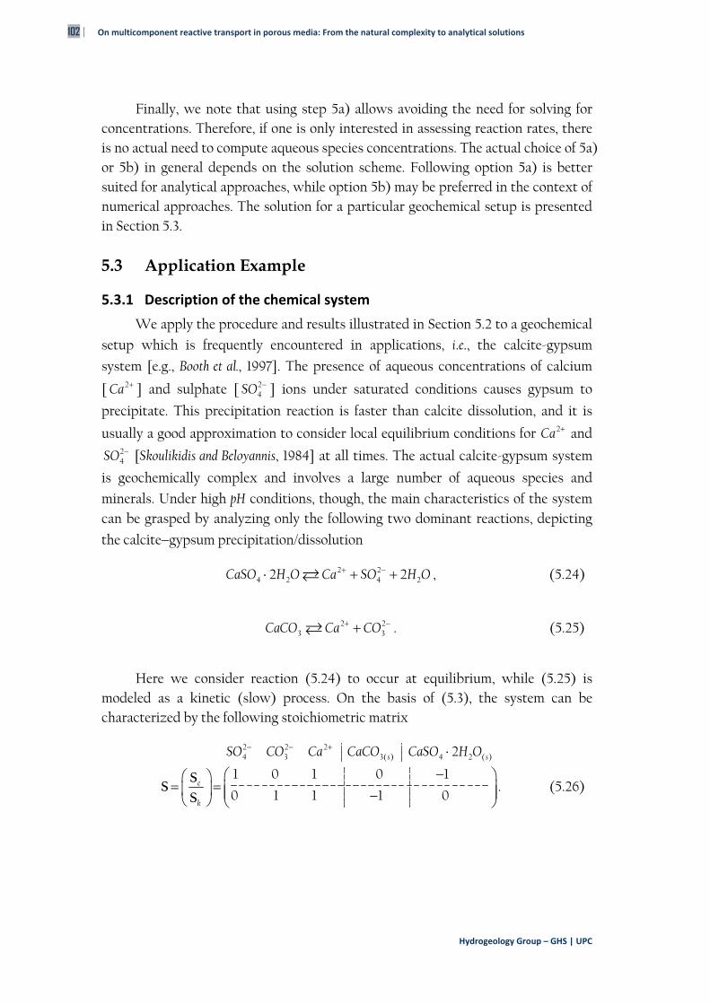
102 | On multicomponent reactive transport in porous media: From the natural complexity to analytical solutions
Hydrogeology Group – GHS | UPC
Finally, we note that using step 5a) allows avoiding the need for solving for concentrations. Therefore, if one is only interested in assessing reaction rates, there is no actual need to compute aqueous species concentrations. The actual choice of 5a) or 5b) in general depends on the solution scheme. Following option 5a) is better suited for analytical approaches, while option 5b) may be preferred in the context of numerical approaches. The solution for a particular geochemical setup is presented in Section 5.3.
5.3 Application Example
5.3.1 Description of the chemical system
We apply the procedure and results illustrated in Section 5.2 to a geochemical
setup which is frequently encountered in applications, i.e., the calcite-gypsum
system [e.g., Booth et al., 1997]. The presence of aqueous concentrations of calcium
[ 2Ca ] and sulphate [ 24SO ] ions under saturated conditions causes gypsum to
precipitate. This precipitation reaction is faster than calcite dissolution, and it is
usually a good approximation to consider local equilibrium conditions for 2Ca and 2
4SO [Skoulikidis and Beloyannis, 1984] at all times. The actual calcite-gypsum system
is geochemically complex and involves a large number of aqueous species and
minerals. Under high pH conditions, though, the main characteristics of the system can be grasped by analyzing only the following two dominant reactions, depicting
the calcitegypsum precipitation/dissolution
2 24 2 4 22 2CaSO H O Ca SO H O , (5.24)
2 23 3CaCO Ca CO . (5.25)
Here we consider reaction (5.24) to occur at equilibrium, while (5.25) is modeled as a kinetic (slow) process. On the basis of (5.3), the system can be characterized by the following stoichiometric matrix
2 2 24 3 3( ) 4 2 ( )2
1 0 1 0 1
0 1 1 1 0
s s
e
k
SO CO Ca CaCO CaSO H O
SS
S. (5.26)
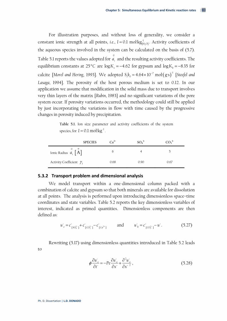
Chapter 5: Simultaneous Equilibrium and Kinetic reaction rates | 103
Ph. D. Dissertation | L.D. DONADO
For illustration purposes, and without loss of generality, we consider a
constant ionic strength at all points, i.e., 2
-1[H O]0.1 mol·kgI . Activity coefficients of
the aqueous species involved in the system can be calculated on the basis of (5.7).
Table 5.1 reports the values adopted for 0
ia and the resulting activity coefficients. The
equilibrium constants at 25 C are log 4.62eK for gypsum and log 8.35kK for
calcite [Morel and Hering, 1993]. We adopted -170 4.64 10 mol· g·ssS k [Steefel and
Lasaga, 1994]. The porosity of the host porous medium is set to 0.12. In our application we assume that modification in the solid mass due to transport involves
very thin layers of the matrix [Rubin, 1983] and no significant variations of the pore system occur. If porosity variations occurred, the methodology could still be applied by just incorporating the variations in flow with time caused by the progressive changes in porosity induced by precipitation.
Table 5.1. Ion size parameter and activity coefficients of the system
species, for -10.1 mol·kgI .
SPECIES Ca2+ SO42- CO3
2-
Ionic Radius 0
ia o
A 6 4 5
Activity Coefficient i 0.68 0.90 0.67
5.3.2 Transport problem and dimensional analysis
We model transport within a one-dimensional column packed with a combination of calcite and gypsum so that both minerals are available for dissolution at all points. The analysis is performed upon introducing dimensionless space–time coordinates and state variables. Table 5.2 reports the key dimensionless variables of interest, indicated as primed quantities. Dimensionless components are then defined as:
2 2 24 3[ ] [ ] [ ]
' ' ' 'e SO CO Cau c c c and 2
3[ ]' ' 'k CO
u c u . (5.27)
Rewriting (5.17) using dimensionless quantities introduced in Table 5.2 leads to
2
2
' ' '' ' 'e e eu u u
Pet x x
, (5.28)
104 | On multicomponent reactive transport in porous media: From the natural complexity to analytical solutions
Hydrogeology Group – GHS | UPC
which we solve with appropriate initial and boundary conditions. By the same token, the equation satisfied by the kinetic component can be written as
2
2
' ' ''
' ' 'k k k
k
u u uPe r
t x x. (5.29)
Table 5.2 Dimensionless parameters and characteristic times
PARAMETER EQUATION
Dimensionless time: 'd
tt
(5.30)
Dimensionless distance: 'x
xl
(5.31)
Diffusive time: 2
D
lD
(5.32)
Advective time: a
lq
(5.33)
Reactive time: *13
0r
K
Sk (5.34)
Péclet number: De
a
qlP
D
(5.35)
Damkölher number: D a
r r
Da Pe
(5.36)
Relative equilibrium reaction constant: *12
1 2
eKK
(5.37)
Relative kinetic reaction constant: *13
1 3
kKK
(5.38)
Dimensionless concentration (i = 1, 2, 3): ' ii
G
cc
K (5.39)
Dimensionless reaction rate (j = e, k):
' dj j
G
r rK
(5.40)
Relative equilibrium constant: *12*13
r
KK
K (5.41)
Dimensionless equilibrium reaction constant: *12
12G
KK
K (5.42)
Dimensionless kinetic reaction constant: *13
13G
KK
K (5.43)
Chapter 5: Simultaneous Equilibrium and Kinetic reaction rates | 105
Ph. D. Dissertation | L.D. DONADO
The expressions for 2[ ]'
Cac , 2
4[ ]'
SOc and 'kr are:
2
212
[ ]
' ' 4'
2k k
Ca
u u Kc
, 2
4
212
[ ]
' ' 4'
2k k
SO
u u Kc
, (5.44)
2 23
14
1 [ ] [ ]2
1' ' 'k r Ca CO
r
r Da K c cK
. (5.45)
Once 'kr is estimated, 'er can be computed as:
2 22 2
[ ] [ ]
2
' '' , 1 ' '
' 'Ca Ca
e k kk k
c cr x t r u
u u x , (5.46)
The derivatives appearing in (5.46) can be computed from(5.44).
5.3.3 Numerical solution
The solution of a particular problem is presented here to illustrate the methodology. The problem analyzed corresponds to a highly diffusive system behavior ( Pe = 0.1) to enhance reaction rates.
Water is initially in equilibrium with respect to calcite and gypsum. The
values adopted for the initial (resident) normalized concentrations are:
2
0
[ ]' 1
t
Cac ,
2
4
0
[ ]' 63.229
t
SOc and
2
3
0
[ ]' 0.0158
t
COc . With these values the initial
concentrations of the conservative and kinetic components are then 0
' 62.2448t
u
and 0
' 62.229t
ku .
Water undersaturated with respect to calcite and saturated with respect to gypsum is continuously introduced in the system at the inlet ( ' 0x ) starting at
time 0t . Concentration values characterizing the chemical signature of the
injected water are: 2[ ] 0
' 0.5Ca x
c , 2
4[ ] 0' 126.458
SO xc and
2
3[ ] 0' 0.00031631
CO xc .
With these concentrations, the boundary conditions are
0' 125.9583
xu and
0' 125.958k x
u , respectively for the conservative and kinetic components. Figure
5.1a juxtaposes the initial and boundary conditions to the corresponding equilibrium
106 | On multicomponent reactive transport in porous media: From the natural complexity to analytical solutions
Hydrogeology Group – GHS | UPC
curves in ( 2[ ]'
Cac , 2
4[ ]'
SOc ) space. The corresponding depiction in ( 2[ ]
'Ca
c , 23[ ]
'CO
c )
space is reported in Figure 5.1b. The set-up corresponds thus to a water initially in chemical equilibrium with the two minerals which is displaced by water which is undersaturated in calcite and saturated in gypsum.
The solution of the reactive transport problem involves solving the non-linear PDE (5.29). We solve it by means of an implicit predictor-corrector approach relying on a forward finite difference and central finite difference approximation respectively for time and space.
5.3.4 Analysis of the results
We start by examining the evolution of the aqueous concentrations of the
species taking part in the kinetic reaction in the ( 2[ ]'
Cac , 2
3[ ]'
COc ) plane. Figure 5.2
depicts the pathlines characterizing the temporal evolution of the state of the chemical system for three selected locations along the column and three values of the
Damkölher number, Da . As a reference, the equilibrium curve is reported, together with the compositions of the initial (resident) and injected water. Pathlines are defined here as the collection of concentration (pair) values that a given point in the column samples with time. In our example, all of them originate from the point corresponding to the chemical signature of the resident water and move leftwards with time (time increases along the direction of the arrows in Figure 5.2). We note
that for small values of Da , i.e., 210Da , the kinetic reaction is very slow, and all pathlines (corresponding to ' 0.05, 0.50, 0.95x ) tend towards the point
corresponding to the injected (boundary) water. This indicates that advection processes dominate with respect to chemical reaction. Notice that the final point (which corresponds to infinite time) of the pathlines does not correspond exactly to that of the injected water, since some amount of reaction takes place.
The picture changes as Da increases. For intermediate values of Da , the final point of a pathline lies somewhere in between the one corresponding to the injected water and the equilibrium curve. We note that pathlines tend to lie closer to the equilibrium curve as the distance between the observation point and the inlet boundary increases. This is associated with the fact that the system has more time to equilibrate. It is interesting to observe that some of the pathlines in Figure 5.2 are
non-monotonic in terms of values of 23[ ]
'CO
c sampled with time. This indicates an
initial decrease in 23[ ]
'CO
c , followed by an increase at a later time. Obviously, the
system is close to equilibrium at all times for very large values of Da , except very close to the inlet point, and pathlines at all points lie near the equilibrium curve.
Moreover, all curves end at a similar (albeit not exactly equal) value of 2[ ]'
Cac . This
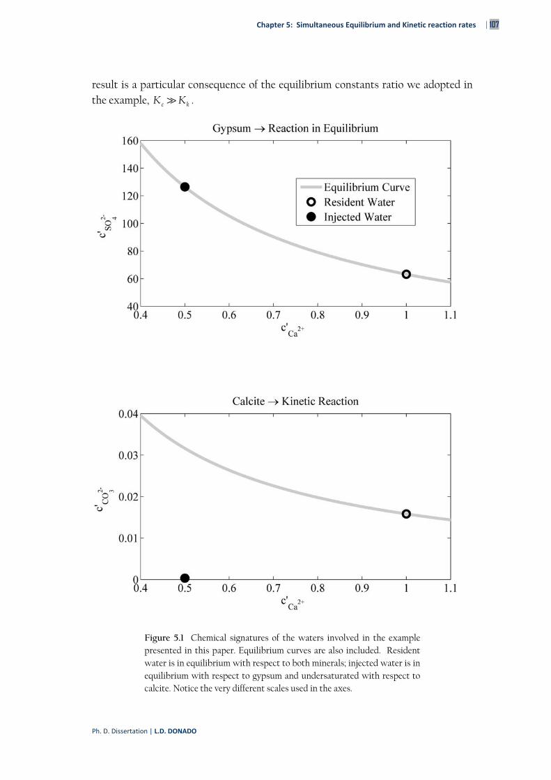
Chapter 5: Simultaneous Equilibrium and Kinetic reaction rates | 107
Ph. D. Dissertation | L.D. DONADO
result is a particular consequence of the equilibrium constants ratio we adopted in the example, e kK K .
Figure 5.1 Chemical signatures of the waters involved in the example presented in this paper. Equilibrium curves are also included. Resident water is in equilibrium with respect to both minerals; injected water is in equilibrium with respect to gypsum and undersaturated with respect to calcite. Notice the very different scales used in the axes.
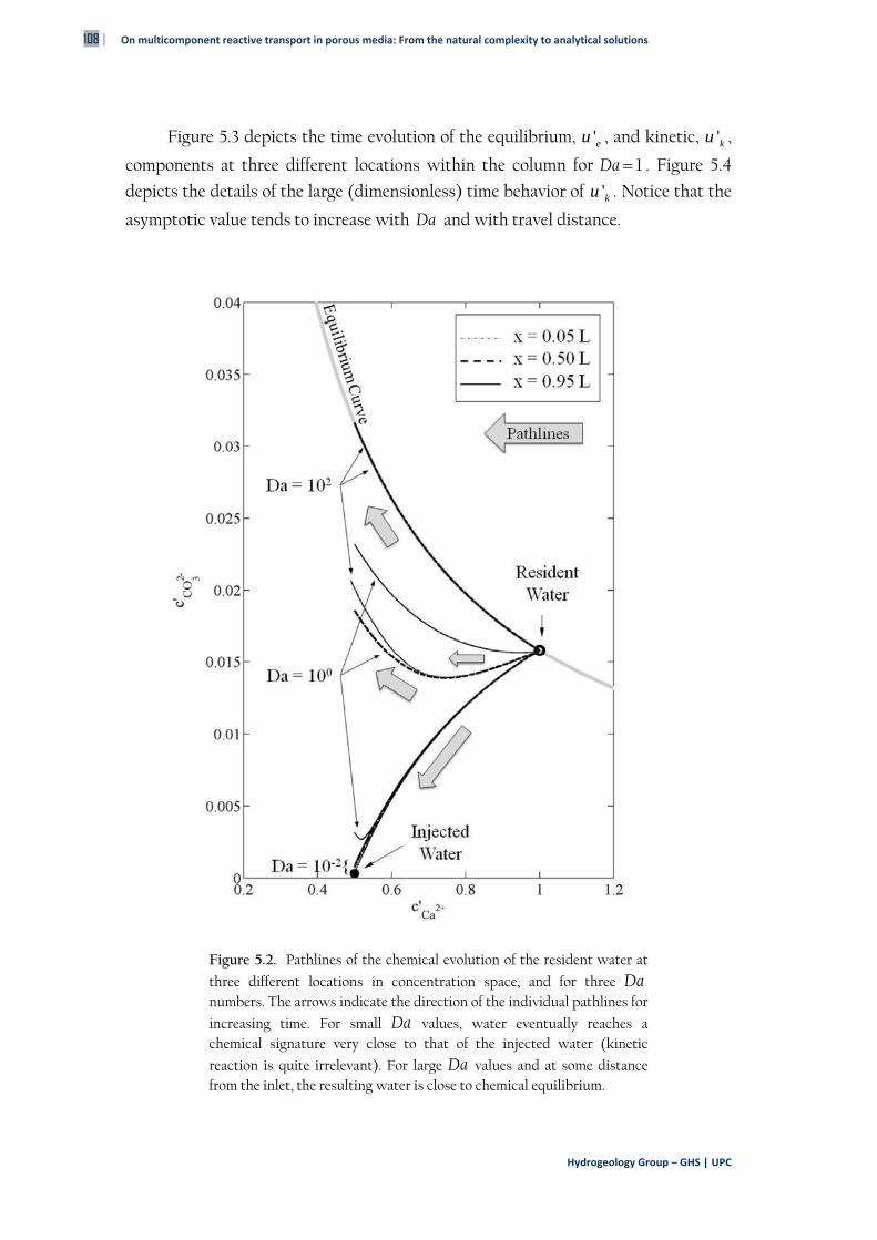
108 | On multicomponent reactive transport in porous media: From the natural complexity to analytical solutions
Hydrogeology Group – GHS | UPC
Figure 5.3 depicts the time evolution of the equilibrium, 'eu , and kinetic, 'ku ,
components at three different locations within the column for 1Da . Figure 5.4
depicts the details of the large (dimensionless) time behavior of 'ku . Notice that the
asymptotic value tends to increase with Da and with travel distance.
Figure 5.2. Pathlines of the chemical evolution of the resident water at
three different locations in concentration space, and for three Da numbers. The arrows indicate the direction of the individual pathlines for
increasing time. For small Da values, water eventually reaches a chemical signature very close to that of the injected water (kinetic
reaction is quite irrelevant). For large Da values and at some distance from the inlet, the resulting water is close to chemical equilibrium.
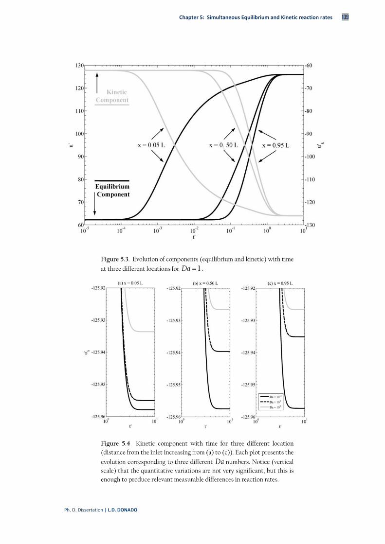
Chapter 5: Simultaneous Equilibrium and Kinetic reaction rates | 109
Ph. D. Dissertation | L.D. DONADO
Figure 5.3. Evolution of components (equilibrium and kinetic) with time
at three different locations for 1Da .
Figure 5.4 Kinetic component with time for three different location (distance from the inlet increasing from (a) to (c)). Each plot presents the
evolution corresponding to three different Da numbers. Notice (vertical scale) that the quantitative variations are not very significant, but this is enough to produce relevant measurable differences in reaction rates.
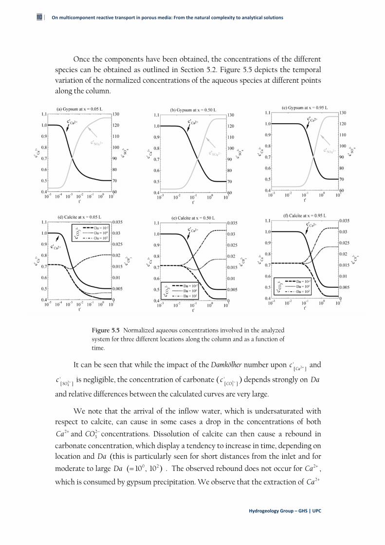
110 | On multicomponent reactive transport in porous media: From the natural complexity to analytical solutions
Hydrogeology Group – GHS | UPC
Once the components have been obtained, the concentrations of the different species can be obtained as outlined in Section 5.2. Figure 5.5 depicts the temporal variation of the normalized concentrations of the aqueous species at different points along the column.
Figure 5.5 Normalized aqueous concentrations involved in the analyzed system for three different locations along the column and as a function of time.
It can be seen that while the impact of the Damkölher number upon 2[ ]'
Cac and
24[ ]
'SO
c is negligible, the concentration of carbonate ( 23[ ]
'CO
c ) depends strongly on Da
and relative differences between the calculated curves are very large.
We note that the arrival of the inflow water, which is undersaturated with respect to calcite, can cause in some cases a drop in the concentrations of both
2Ca and 23CO concentrations. Dissolution of calcite can then cause a rebound in
carbonate concentration, which display a tendency to increase in time, depending on location and Da (this is particularly seen for short distances from the inlet and for
moderate to large Da 0 2( 10 , 10 ) . The observed rebound does not occur for 2Ca ,
which is consumed by gypsum precipitation. We observe that the extraction of 2Ca
Chapter 5: Simultaneous Equilibrium and Kinetic reaction rates | 111
Ph. D. Dissertation | L.D. DONADO
causes further dissolution of calcite, to the point that for high Da or short travel
distances the asymptotic concentration of 23CO is higher than that of either input or
resident waters.
The temporal behavior of normalized kinetic and equilibrium reaction rates are shown in Figure 5.6. Gypsum precipitation, er , despite occurring at equilibrium,
is (non-monotonically) affected by Da , since it depends on the interplay between transport and reaction characteristic times, which ultimately govern the evolution of
the system. In the limit for large Damkölher numbers the equilibrium reaction rate
tends to the solution presented by De Simoni et al. [2005] for a bi-molecular reaction
system. An important feature of the system is that re tends to (a negative) non-zero (albeit in some cases very close to zero) asymptotic values for large times. This is particularly clear for intermediate values of Da at ' 0.5 x (Figures 5.6b, e). Likewise, the kinetic reaction rate depends on Da and tends to a positive asymptotic value (Figures 6d, e, f). This is equivalent to state that the system is always active also in the limit for large times, as a kinetic reaction always takes place in order to preserve
local equilibrium conditions. In short, the actual late-time concentrations 2[ ]'
Cac and
24[ ]
'SO
c are always different (albeit only slightly, in the analyzed scenario) from those
of the input (external) water.
5.4 General Formulation
We now extend the methodology illustrated in Section 5.2 to describe multispecies transport processes in the presence of generic homogeneous and classical heterogeneous reactions. Chemical equilibrium is defined in terms of the mass action law, relating reactants and products. Following the notation introduced in Section 5.2, one can write
*log log logea a K K S c , (5.47)
here, eaS is a e saN N matrix ( eN and saN respectively being the number of
equilibrium reactions and the number of aqueous species in the system) containing the stoichiometric coefficient of equilibrium reactions; ac is the vector of
concentrations of aqueous species; K and *K respectively are the vectors of
equilibrium and equivalent equilibrium constants; is the vector of activity coefficients. The stoichiometry of kinetic reactions is typically included in the kinetic stoichiometric matrix, kS of size k sN N ( kN and sN respectively being the
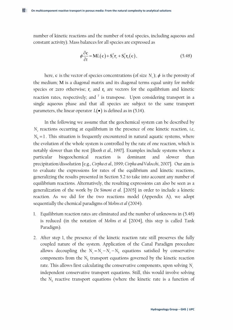
112 | On multicomponent reactive transport in porous media: From the natural complexity to analytical solutions
Hydrogeology Group – GHS | UPC
number of kinetic reactions and the number of total species, including aqueous and constant activity). Mass balances for all species are expressed as
T Te e k kL
t
c
M c S r S r c , (5.48)
here, c is the vector of species concentrations (of size sN ); is the porosity of
the medium; M is a diagonal matrix and its diagonal terms equal unity for mobile species or zero otherwise; er and kr are vectors for the equilibrium and kinetic
reaction rates, respectively; and T is transpose. Upon considering transport in a single aqueous phase and that all species are subject to the same transport
parameters, the linear operator L is defined as in (5.14).
In the following we assume that the geochemical system can be described by
eN reactions occurring at equilibrium in the presence of one kinetic reaction, i.e,
1kN . This situation is frequently encountered in natural aquatic systems, where
the evolution of the whole system is controlled by the rate of one reaction, which is
notably slower than the rest [Booth et al., 1997]. Examples include systems where a particular biogeochemical reaction is dominant and slower than
precipitation/dissolution [e.g., Cirpka et al., 1999; Cirpka and Valocchi, 2007]. Our aim is to evaluate the expressions for rates of the equlibrium and kinetic reactions, generalizing the results presented in Section 5.2 to take into account any number of equilibrium reactions. Alternatively, the resulting expressions can also be seen as a
generalization of the work by De Simoni et al. [2005] in order to include a kinetic reaction. As we did for the two reactions model (Appendix A), we adopt
sequentially the chemical paradigms of Molins et al (2004).
1. Equilibrium reaction rates are eliminated and the number of unknowns in (5.48)
is reduced (in the notation of Molins et al. [2004], this step is called Tank Paradigm).
2. After step 1, the presence of the kinetic reaction rate still preserves the fully coupled nature of the system. Application of the Canal Paradigm procedure allows decoupling the c s e kN N N N equations satisfied by conservative
components from the kN transport equations governed by the kinetic reaction
rate. This allows first calculating the conservative components, upon solving cN
independent conservative transport equations. Still, this would involve solving the kN reactive transport equations (where the kinetic rate is a function of
Chapter 5: Simultaneous Equilibrium and Kinetic reaction rates | 113
Ph. D. Dissertation | L.D. DONADO
species concentrations) together with the eN chemical expressions (5.47) and
the cN definitions of conservative components.
3. By applying the River and Aquifer Paradigms procedure, it is possible to eliminate both the kinetic and constant activity species from the system. This leads to a fully decoupled problem that can be solved in steps similar to those proposed in Section 5.2 for the two-reactions model. This procedure yields the space-time distribution of equilibrium and kinetic reaction rates from the numerical solution of (5.48), once the vector c is known.
Figure 5.6 Normalized kinetic reaction rate and normalized equilibrium reaction rate at three different locations along the column and as a function of time. Notice the very different vertical scales in each plot
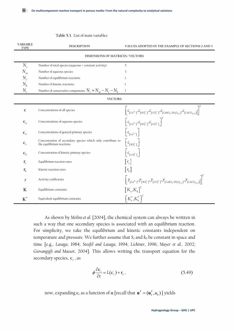
114 | On multicomponent reactive transport in porous media: From the natural complexity to analytical solutions
Hydrogeology Group – GHS | UPC
Table 5.3. List of main variables
VARIABLE TYPE
DESCRIPTION VALUES ADOPTED IN THE EXAMPLE OF SECTIONS 2 AND 3
DIMENSIONS OF MATRICES / VECTORS
sN Number of total species (aqueous + constant activity) 5
saN Number of aqueous species 3
eN Number of equilibrium reactions 1
kN Number of kinetic reactions 1
cN Number of conservative components c sa e kN N N N 1
VECTORS
c Concentrations of all species 2 2 2
4 3 4 2 ( ) 3( )[ ] [ ] [ ] [ 2 ] [ ], , , ,
s s
T
Ca SO CO CaSO H O CaCOc c c c c
ac Concentrations of aqueous species 2 2 2
4 3[ ] [ ] [ ], ,
T
Ca SO COc c c
'ac Concentrations of general primary species 2[ ]Cac
ec Concentration of secondary species which only contribute to the equilibrium reactions 2
4[ ]SOc
kc Concentration of kinetic primary species 23[ ]CO
c
er Equilibrium reaction rates er
kr Kinetic reaction rates kr
Activity coefficients 2 2 2
4 3 4 2 ( ) 3( )[ ] [ ] [ ] [ 2 ] [ ], , , ,
s s
T
Ca SO CO CaSO H O CaCO
K Equilibrium constants ,T
e kK K
*K Equivalent equilibrium constants * *,T
e kK K
As shown by Molins et al. [2004], the chemical system can always be written in such a way that one secondary species is associated with an equilibrium reaction. For simplicity, we take the equilibrium and kinetic constants independent on
temperature and pressure. We further assume that Ss and k0 be constant in space and
time [e.g., Lasaga, 1984; Steefel and Lasaga, 1994; Lichtner, 1996; Mayer et al., 2002;
Giovangigli and Massot, 2004]. This allows writing the transport equation for the
secondary species, ec , as
( )cc eL
t c
c r , (5.49)
now, expanding ce as a function of u [recall that ( , )T Te kuu u ] yields
Chapter 5: Simultaneous Equilibrium and Kinetic reaction rates | 115
Ph. D. Dissertation | L.D. DONADO
2
2( ) · ·tc c
eLt
c u c
u u D u ru u
, (5.50)
where the left hand side is zero for all components but ku , which satisfies
equation (5.19). Substituting (5.19) into (5.50) yields
2
2· ·tc c
e kk
ru
c cr u D u
u. (5.51)
In the absence of the kinetically driven behavior, one immediately recovers
from (5.51) the expression of De Simoni et al. [2005], where the reaction is solely driven by mixing.
5.5 Conclusions
Our work leads to the following major conclusions:
1. The methodology we propose allows obtaining exact explicit expressions of the space-time distribution of reaction rates when the geochemical system can be described by eN reactions occurring at equilibrium in the presence of
one kinetic reaction. The equilibrium reaction rate is then expressed as a function of a mixing-related term, the distribution of (conservative and kinetic) components and the kinetic reaction rate.
2. The complete analysis of the analyzed reactive transport problem entails deconstructing it according to a sequence of decoupled steps. A key point of the procedure is that it eliminates the need to compute aqueous concentrations if one is only interested in assessing reaction rates. As compared to formulations previously proposed in the literature to solve multispecies transport problems in the presence of a generic number of
reactions [e.g., Molins et al., 2004], the method we adopt is simpler and more concise. The critical point in the procedure is the computation of the reactive component, ku , which satisfies a highly non-linear partial differential
equation. In general, the latter should be solved numerically. It follows that the advantages associated with our procedure (solving an individual non-linear equation in front of solving the complete coupled system of non-linear equations) should be further explored in practical applications.
116 | On multicomponent reactive transport in porous media: From the natural complexity to analytical solutions
Hydrogeology Group – GHS | UPC
3. The resulting expressions are applied to a geochemical setup which is
frequently encountered in applications, i.e., the calcite-gypsum system. The salient features of the latter are typically described by two chemical reactions. The transport of reactive species is then solved to simulate the dissolution of calcite in the presence of water geochemically equilibrated with gypsum within a one-dimensional column. The solution is offered in terms of relevant dimensionless parameters controlling the system, highlighting the role of the heavily non-linear interplay between characteristic transport and reaction times. A key finding is that the system is always active in the limit for large times, as the reactants kinetically interact in order to preserve local equilibrium conditions.
chapter
On multicomponent reactive transport in porous media: From the natural complexity to analytical solutions

(This page intentionally left blank.)
Chapter 6: Summary and Conclusions | 117
Ph. D. Dissertation | L.D. DONADO
Chapter 6
Summary and Conclusions
6 SUMMARY AND CONCLUSIONS
he dissertation was focused on the analysis and characterization of the transport of non-conservatives solutes in the geological media. The latter is very complex due to geological processes of genesis and
formation. Indeed, natural media as fractured rocks or aquifers presents high variability of their hydrodynamic properties. This variability adds high complexity in the understanding of all processes and phenomena that occurs on them.
Effective dynamics have been stated by several authors as a modeling approach for flow and transport in heterogeneous media. These dynamics can be fully-defined in three main groups: (i) multirate mass transfer, MRMT, (ii) continuous time random walk, CTRW and (iii) fractional advection dispersion equations, FADE.
Between different geological media, fractured media presents a special interest in the scientific community due to its usefulness in the storage of nuclear wastes because of its low permeability. Radionuclides are a very non-conservative type of solute that can be affected by several types of reactions. Reactions can be defined in function of its characteristic time as instantaneous or slow. The former are very fast in comparison with transport characteristic time and the latter are slow and the reaction characteristic time is relatively similar to transport characteristic time. If
T
118 | On multicomponent reactive transport in porous media: From the natural complexity to analytical solutions
Hydrogeology Group – GHS | UPC
reaction is slow, the hydrogeological media is not in equilibrium, and the equations for modeling the multicomponent system are not linear and not homogeneous.
This research was carried out in four stages. The first one consists on the inverse modeling of groundwater flow and solute transport in fractured media, represented by means of Discrete Fracture Network as conceptual model. The second consist on a definition of an analytical expression to compute equilibrium reaction rates in multi-species reactive transport system in a heterogeneous media. The heterogeneity of the media was based on MRMT effective dynamics. Third stage of the dissertation was focused on the establishment of a semi-analytical solution for the reaction rates in a system under non-equilibrium conditions. And finally, last stage was the generation of analytical expression for reaction rates in a system with the presence of any quantity of equilibrium reactions and one kinetic reaction. A summary of the main results and future work lines of each stage are presented as follows.
6.1 Inverse modeling with DFN
6.1.1 Main Results
Groundwater flow and solute transport were modeled in a fractured media via DFN approach. A total number of 100 synthetic realizations of DFN were generated based on the probability distributions of the field geological properties. DFN represents fractures as discs that are associated to fracture families to simplify the total number of parameters to be calibrated.
Hydraulic and tracer tests were calibrated by means of inverse problem with TRANSIN II. Results of this modeling permit to conclude that DFN present similar or best results to previous modeling with an Equivalent Porous Media. DFN poses as a more realistic definition of the fractured media, but generate a gigantic quantity of hydrodynamic parameters to compute and calibrate.
Transport in this type of media is a challenging problem due to behavior of solutes and their interaction with the rock matrix. Breakthrough curves of deuterium shows tailing that typical fickian solutions cannot adequately represent. The inverse model demonstrates that adding matrix diffusion to the advection-dispersion mass balance equation, BTC have an extraordinary fitting. This type of behavior is related to memory effects caused by the heterogeneity of the media.
Statistical analysis of the different calibrated hydraulic parameters (hydraulic conductivity and specific storativity) shows that every family has a monomodal distribution of their hydrodynamic parameter. This is called effective parameter. In
Chapter 6: Summary and Conclusions | 119
Ph. D. Dissertation | L.D. DONADO
contrast, when all the values are analyzed, parameters show a bimodal distribution. These parameters are defined as ensemble. Effective parameter does not represent
6.1.2 Outlook
Additional research into the influence of the connectivity of the channels will provide a reduction of the broad band of the conductance matrix. It is suggested that there must be an effective network of channels that conducts all the water. A more extensive study of it can be done applying percolation theory. An effective conductive network will reduce the computation cost of the calibration models.
DFN approach is generally related to a model in which the location of fractures
inside the matrix are fully defined [e.g., MacQuarrie and Mayer, 2005]. It may be possible to condition the generated networks to hard data achieved from borehole data logs.
It is suggested that a statistical analysis of transport parameters could be also undertaken. It will offer a definition of effective and ensemble values for transport parameters. An important issue that can be solved is the scale problem because the greater part of multi-specie reactive transport problems are limited for it.
Tailings of the breakthrough curves are caused when diffusion dominates the processes. An application of an effective dynamics approach can be carried out in this type of media. The main idea is to represent the heterogeneity of the media and its effect on the diffusive processes. The effective dynamics will represent low and high permeability zones and their interaction, behavior that dominates the transport processes.
6.2 Reaction rates for mixing-controlled reaction in multi-continuum media
6.2.1 Main Results
Based on the evidence of tailing on BTC, an effective dynamic with memory effects was implemented. Heterogeneous media is visualized as a multiple overlapping continua with different types of permeability. MRMT approach was used as effective dynamics.
This type of approach permits to represent the influence of heterogeneity in hydrodynamic processes in the media without having into account that implemented scaling method for the definition of effective or ensemble parameters.
In this approach, the medium heterogeneity is represented by the distribution of solute retention times. The used approach has permitted to achieve an analytical
120 | On multicomponent reactive transport in porous media: From the natural complexity to analytical solutions
Hydrogeology Group – GHS | UPC
expression for compute the reaction rates in both mobile and immobile zones. This analytical expression identifies three different contributions: (i) an identical term
that represent local dispersive mixing in the mobile region [De Simoni et al., 2005], (ii) the term that represent mixing caused by mass transfer among zones, and (iii) a term that represent the reaction in the set of immobile zones.
Heterogeneity of media is characterized by a set of mobile and immobile zones. When an advective-dispersive multi-specie transport is presented in the mobile zones, the unique mechanism that induces non equilibrium conditions is local dispersion. With the additional presence of mass transfer with immobile waters, mixing is achieved. This induces non-equilibrium and reactions too.
For local dispersive mixing, the relevant time scale is given by the dispersion time, while for mass transfer mixing, the time scale is defined by the reaction time. The time for the system to reach global equilibrium can be significantly increased. Such mechanisms can not be captured by a macro-dispersion model, which would lead to an underestimation of the total reaction taking place. As consequence, the degree of heterogeneity, as well the mass transfer rates has an important impact in the total reaction rate.
In advective dominated cases, the majority of the reaction takes place in the immobile zones. It means that the heterogeneity defines the reaction and mixing. An advantage of this type of approach, is the correct description of the reaction rate, with no underestimation caused by up-scaling parameters as macrodispersive approach.
6.2.2 Outlook
From the point of view of practical engineering it will be important to follow this type of approach in natural media to obtain corroboration of the analytical results.
Multi-rate mass transfer approach poses as an ideal model for representing mixing in micro-scale, but its applicability in large-scale media is argued by several senior authors. Numerical modeling carried out by Hydrogeology Group in recent years demonstrates that this type of approach is useful for the differentiation among spreading and mixing.
The following stage of the research could be an experimental program to verify that this analytical solution really quantifies mixing effects, therefore a correct prediction of plume shapes and remediation techniques.
Chapter 6: Summary and Conclusions | 121
Ph. D. Dissertation | L.D. DONADO
6.3 Transport-Controlled Reaction Rates Under Local Non-Equilibrium Conditions
6.3.1 Main Results
A reaction can be defined by its characteristic time as slow or instantaneous. In an advective-dispersive transport system, it depends on the relationship with the transport characteristic time. It means that when the transport time is similar or greater that the reaction time, the reaction can be treated as instantaneous. In contrary, when reaction time is larger than transport one, reaction is not in equilibrium and is defined by a kinetic law. Kinetic reaction adds non-linearity to mathematical models. This part of the dissertations shows an analytical solution for reaction rate in multi-species reactive transport under local non-equilibrium conditions.
One of the main results consists on an analysis of the influence on local non-equilibrium conditions in the reaction. This study defines the ratio among transport and reaction characteristic times. When this ratio is very small, reaction tends to be
in equilibrium and the solution is the same stated one [De Simoni et al., 2005], but if this ratio is greater, reaction rates can be underestimated, therefore all the plumes hydrodynamics.
6.3.2 Outlook
As a result of this research, the impact of larger deviations from local equilibrium (typical mass transfer time smaller than the reaction time scale) needs to be analyzed by a full (numerical) solution of the non-linear partial differential equation and comparison to experiments and direct numerical simulations.
6.4 Simultaneous Equilibrium and Kinetic Reaction Rate in Porous Media
6.4.1 Main Results
The last stage of the dissertation was focused on achieving analytical solutions for reaction rates in a more realistic situation, with the presence of two types of reactions: several ones in equilibrium and one kinetic. This work leads to the following results.
Exact and explicit expressions to compute reaction rates distributions in space and time for the defined geochemical system. Equilibrium reaction rates are
122 | On multicomponent reactive transport in porous media: From the natural complexity to analytical solutions
Hydrogeology Group – GHS | UPC
expressed in terms of the mixing, the kinetic reaction rate and the distribution of components.
This study proposes a methodology to compute reaction rates, eliminating the need to compute aqueous concentrations, because reaction rates and their relationship with component define the mixing processes.
The solution is offered in terms of relevant dimensionless parameters controlling the system, highlighting the role of the heavily non-linear interplay between characteristic transport and reaction times. A key result is that the system is always active in the limit for large times, as the reactants kinetically interact in order to preserve local equilibrium conditions.
6.4.2 Outlook
It follows that the advantages associated with the implemented procedure (solving an individual non-linear equation in front of solving the complete coupled system of non-linear equations) should be further explored in practical applications.
The critical point is the procedure of computation of the kinetic component. In general, it is achieved by means of numerical solution of a non-linear and non-homogeneous differential partial equation. A sophisticated numerical approach must be implemented for solving more complex problems.
chapter
On multicomponent reactive transport in porous media: From the natural complexity to analytical solutions

(This page intentionally left blank.)
Chapter 7: References | 123
Ph. D. Dissertation | L.D. DONADO
Chapter 7
References
7 REFERENCES
Azaroual, M., C. Kervévan, M. V. Durance, S. Brochot, and P. Durst (2003), SCALE2000 user’s manual, edited, p. 57, BRGM, Orléans, France.
Baecher, G. B., and N. A. Lanney (1978), Trace length biases in joint surveys, paper presented at 19th U.S. Symposium on Rock Mechanics, AIME, 56-65.
Bear, J. (1972), Dynamics of fluids in porous media, Dover Publications, Inc., New York. Bear, J. (1993), Modeling flow and contaminant transport in fractured rocks, in Flow and contaminant transport in
fractured media, edited by J. Bear, C. F. Tsang and G. De Marsily, Academic Press, Inc, San Diego, California. Bear, J., and B. Berkowitz (1987), Groundwater flow and pollution in fractured rock aquifers, in Developments of
Hydraulic Engineering, edited by I. P. Novak, Elsevier. Benson, D. A., S. W. Wheatcraft, and M. M. Meerschaert (2000a), Application of a fractional advection-
dispersion equation, Water Resour. Res., 36(6), 1403-1412 Benson, D. A., S. W. Wheatcraft, and M. M. Meerschaert (2000b), The fractional-order governing equation of
Levy motion, Water Resour. Res., 36(6), 1413-1423 Berkowitz, B. (2002), Characterizing flow and transport in fractured geological media: A review, Adv. Water
Resour., 25(8-12), 861-884 Berkowitz, B., J. Bear, and C. Braester (1988), Continuum Models for Contaminant Transport in Fractured
Porous Formations, Water Resour. Res., 24(8), 1225-1236 Berkowitz, B., A. Cortis, M. Dentz, and H. Scher (2006), Modeling non-Fickian transport in geological
formations as a continuous time random walk, Rev. Geophys., 44(2), RG2003, doi:10.1029/2005RG000178. Berkowitz, B., S. Emmanuel, and H. Scher (2008), Non-Fickian transport and multiple-rate mass transfer in
porous media, Water Resour. Res., 44(3), W03402, doi:10.1029/2007WR005906. Berkowitz, B., and H. Scher (1995), On Characterization of Anomalous-Dispersion in Porous and Fractured
Media, Water Resour. Res., 31(6), 1461-1466 Berkowitz, B., and H. Scher (1998), Theory of anomalous chemical transport in random fracture networks, Phys.
Rev. E: Stat. Phys., Plasmas, Fluids,, 57(5), 5858-5869 Berkowitz, B., and H. Scher (2001), The role of probabilistic approaches to transport theory in heterogeneous
media, Transport Porous Med., 42(1-2), 241-263 Bodin, J., F. Delay, and G. de Marsily (2003a), Solute transport in a single fracture with negligible matrix
permeability: 1. fundamental mechanisms, Hydrogeol. J., 11(4), 418-433 Bodin, J., F. Delay, and G. de Marsily (2003b), Solute transport in a single fracture with negligible matrix
permeability: 2. mathematical formalism, Hydrogeol. J., 11(4), 434-454
124 | On multicomponent reactive transport in porous media: From the natural complexity to analytical solutions
Hydrogeology Group – GHS | UPC
Bodin, J., G. Porel, F. Delay, F. Ubertosi, S. Bernard, and J. R. de Dreuzy (2007), Simulation and analysis of solute transport in 2D fracture/pipe networks: The SOLFRAC program, J. Contam. Hydrol., 89(1-2), 1-28
Bonnet, E., O. Bour, N. E. Odling, P. Davy, I. Main, P. Cowie, and B. Berkowitz (2001), Scaling of fracture systems in geological media, Rev. Geophys., 39(3), 347-383
Booth, J., Q. Hong, R. G. Compton, K. Prout, and R. M. Payne (1997), Gypsum overgrowths passivate calcite to acid attack, J. Colloid Interf. Sci., 192(1), 207-214
Borden, R. C., and P. B. Bedient (1986), Transport of Dissolved Hydrocarbons Influenced by Oxygen-Limited Biodegradation .1. Theoretical Development, Water Resour. Res., 22(13), 1973-1982
Cacas, M. C., E. Ledoux, G. de Marsily, B. Tillie, A. Barbreau, E. Durand, B. Feuga, and P. Peaudecerf (1990), Modeling Fracture Flow With a Stochastic Discrete Fracture Network: Calibration and Validation 1. The Flow Model, Water Resour. Res., 26(3), 479–489
Carrera, J., and S. P. Neuman (1986a), Estimation of Aquifer Parameters under Transient and Steady-State Conditions .1. Maximum-Likelihood Method Incorporating Prior Information, Water Resour. Res., 22(2), 199-210
Carrera, J., and S. P. Neuman (1986b), Estimation of Aquifer Parameters under Transient and Steady-State Conditions .2. Uniqueness, Stability, and Solution Algorithms, Water Resour. Res., 22(2), 211-227
Carrera, J., and S. P. Neuman (1986c), Estimation of Aquifer Parameters under Transient and Steady-State Conditions .3. Application to Synthetic and Field Data, Water Resour. Res., 22(2), 228-242
Carrera, J., X. Sanchez-Vila, I. Benet, A. Medina, G. Galarza, and J. Guimera (1998), On matrix diffusion: formulations, solution methods and qualitative effects, Hydrogeol. J., 6(1), 178-190
Cederberg, G. A., R. L. Street, and J. O. Leckie (1985), A Groundwater Mass-Transport and Equilibrium Chemistry Model for Multicomponent Systems, Water Resour. Res., 21(8), 1095-1104
Chang, J., and Y. C. Yortsos (1990), Pressure transient analysis of fractal reservoirs, SPE Formation Evaluation361 Cirpka, O. A., E. O. Frind, and R. Helmig (1999), Numerical simulation of biodegradation controlled by
transverse mixing, J. Contam. Hydrol., 40(2), 159-182 Cirpka, O. A., A. Olsson, Q. S. Ju, M. A. Rahman, and P. Grathwohl (2006), Determination of transverse
dispersion coefficients from reactive plume lengths, Ground Water, 44(2), 212-221 Cirpka, O. A., and A. J. Valocchi (2007), Two-dimensional concentration distribution for mixing-controlled
bioreactive transport in steady state, Adv. Water Resour., 30(6-7), 1668-1679 Clement, T. P. (2001), Generalized solution to multispecies transport equations coupled with a first-order
reaction network, Water Resour. Res., 37(1), 157-163 Clement, T. P., Y. Sun, B. S. Hooker, and J. N. Petersen (1998), Modeling multispecies reactive transport in
ground water, Ground Water Monit. Remed., 18(2), 79-92 Committee on Fracture Characterization and Fluid Flow, U. N. R. C. (1996), Rock Fractures and Fluid Flow:
Contemporary Understanding and Applications, National Academy Press, Washington. Connaughton, D. F., J. R. Stedinger, L. W. Lion, and M. L. Shuler (1993), Description of Time-Varying
Desorption-Kinetics - Release of Naphthalene from Contaminated Soils, Environ. Sci. Tech., 27(12), 2397-2403
Conrad, F., and C. Jacquin (1973), Répresentation d’un réseau bidimensionnel de -fractures par un modéle probabiliste: Application au calcul des grandeurs géométriques des blocs matriciels, Reveu de l'Institute Français du Pétrole, 28(6), 843-890
Coudrainribstein, A., and F. M. M. Morel (1987), Transport Modeling of Major Reactive Elements in a Variable Temperature-Field - Methodology and Simple Examples, Bull. Soc. Geol. Fr., 3(5), 1009-1017
Cushman, J. H., and T. R. Ginn (2000), Fractional advection-dispersion equation: A classical mass balance with convolution-Fickian flux, Water Resour. Res., 36(12), 3763-3766
Cvetkovic, V., J. O. Selroos, and H. Cheng (1999), Transport of reactive tracers in rock fractures, J. Fluid. Mech., 378335-356
D'Alessandro, M., J. Guimerà, F. Mousty, and A. Yllera De Llano (1995), In situ migration tests at El Berrocal site with conservative isotopic tracers: Laboratory and field results from phase 1 of the project, El Berrocal Project, Topical report No. 15, Intera, UK.
D'Alessandro, M., F. Mousty, G. Bidoglio, J. Guimera, I. Benet, X. Sanchez-Vila, M. Garcia Gutierrez, and A. Yllera De Llano (1997a), Field tracer experiment in a low permeability fractured medium: results from El Berrocal site, J. Contam. Hydrol., 26(1-4), 189-201, doi:10.1016/S0169-7722(96)00068-X
D'Alessandro, M., F. Mousty, G. Bidoglio, J. Guimera, I. Benet, X. Sanchez-Vila, M. Garcia Gutiérrez, and A. Yllera De Llano (1997b), Field tracer experiment in a low permeability fractured medium: results from El Berrocal site, J. Contam. Hydrol., 26(1-4), 189-201, doi:10.1016/S0169-7722(96)00068-X
Dagan, G. (1986), Statistical-Theory of Groundwater-Flow and Transport - Pore to Laboratory, Laboratory to Formation, and Formation to Regional Scale, Water Resour. Res., 22(9), S120-S134
De Simoni, M., J. Carrera, X. Sanchez-Vila, and A. Guadagnini (2005), A procedure for the solution of multicomponent reactive transport problems, Water Resour. Res., 41(11), W11410, doi:10.1029/2005WR004056.
De Simoni, M., J. Carrera, X. Sanchez-Vila, and M. Saaltink (2007), A mixing ratios-based formulation for multicomponent reactive transport, Water Resour. Res., 43(7), W07419, doi:10.1029/2006WR005256.
Chapter 7: References | 125
Ph. D. Dissertation | L.D. DONADO
Dentz, M., and B. Berkowitz (2003), Transport behavior of a passive solute in continuous time random walks and multirate mass transfer, Water Resour. Res., 39(5), 1111, doi:10.1029/2001WR001163.
Dentz, M., A. Cortis, H. Scher, and B. Berkowitz (2004), Time behavior of solute transport in heterogeneous media: transition from anomalous to normal transport, Adv. Water Resour., 27(2), 155-173
Dershowitz, W. S. (1984), Rock joint systems, 764 pp, Massachusetts Institute of Technology, Cambridge. Dershowitz, W. S., and H. H. Einstein (1988), Characterizating rock joint geometry with joint system models,
Roc Mech. Rock Eng., 21(1), 21-51 Dershowitz, W. S., P. Wallmann, and S. Kindred (1991), Discrete Fracture Network for the Stripa Site
Characterization and Validation Drift Inflow Predictions, 140 pp, SKB Stripa Technical Report, TR-91-16, SKB, Swedish Nuclear Power and Waste Management Co., Stockholm.
Deutsch, C. V., and P. W. Cockerham (1994), Practical considerations in the application of simulated annealing to stochastic simulation, Math. Geol., 26(1), 67-82
Donado, L. D., A. Guadagnini, X. Sanchez-Vila, and J. Carrera (Submmited-a), Solution for multicomponent reactive transport under equilibrium and kinetic reactions, Water Resour. Res.
Donado, L. D., E. Ruiz, X. Sanchez-Vila, F. J. Elorza, C. Bajos, and A. Vela-Guzman (2006), Calibration of hydraulic and tracer tests in fractured media represented by a DFN Model, paper presented at Calibration and Reliability in Groundwater Modelling: From Uncertainty to Decision Making. MODELCARE 2005, IAHS Publication, 316 + xii, The Hague, The Netherlands, 2005.
Donado, L. D., X. Sanchez-Vila, M. Dentz, J. Carrera, and D. Bolster (Submmited-b), Multi-component reactive transport in multi–continuum media, Water Resour. Res.
Durlofsky, L. J. (1991), Numerical Calculation of Equivalent Grid Block Permeability Tensors for Heterogeneous Porous Media, Water Resour. Res., 27(5), 699-708
Elorza, F. J., R. Nita, F. Flórez, C. Paredes, L. Vives, E. Ruiz, X. Sanchez-Vila, J. Carrera, S. Martin, A. Muñoz, G. De Vicente, A. Vela, and C. Bajos (2003), Simulación hidrogeológica estocástica de medios geológicos gracturados, in Geoestadística y modelos matemáticos en hidrogeología, edited by J. Mateu, M. Chica-Olmo and I. Morell, p. 312, Universitat Jaume I, Castellón.
Fernandez-Garcia, D., X. Sanchez-Vila, and A. Guadagnini (2008), Reaction rates and effective parameters in stratified aquifers, Adv. Water Resour., 31(10), 1364-1376, doi: 10.1016/j.advwatres.2008.07.001
Fisher, N. I., T. Lewis, and B. J. J. Embleton (1987), Statistical analysis of spherical data, Cambridge University Press. Friedly, J. C., and J. Rubin (1992), Solute Transport with Multiple Equilibrium-Controlled or Kinetically
Controlled Chemical-Reactions, Water Resour. Res., 28(7), 1935-1953 Garcia Gutierrez, M., J. Guimera, A. Yllera De Llano, A. Hernandez Benitez, J. Humm, and M. Saaltink (1997),
Tracer test at El Berrocal site, Journal of Contaminant Hydrology, 26(1-4), 179-188, doi:10.1016/S0169-7722(96)00067-8.
Gelhar, L. W., and C. L. Axness (1983), 3-Dimensional Stochastic-Analysis of Macrodispersion in Aquifers, Water Resour. Res., 19(1), 161-180
Geman, S., and D. Geman (1984), Stochstic relaxation, Gibbs distributions, and the bayesian restoration of images, IEEE T. Pattern Anal., 6(6), 721-741
Giovangigli, V., and M. Massot (2004), Entropic structure of multicomponent reactive flows with partial equilibrium reduced chemistry, Math. Meth. Appl. Sci., 27(7), 739-768
Guadagnini, A., X. Sanchez-Vila, M. Saaltink, M. Bussini, and B. Berkowitz (2009), Application of a mixing-ratios based formulation to model mixing-driven dissolution experiments Adv. Water Resour., 32(5), 756-766, doi:10.1016/j.advwatres.2008.07.005.
Guimera, J., L. Vives, M. Saaltink, P. Tume, J. Carrera, P. Meiers, and B. Ruiz (1996), Numerical modelling of pumping tests in a fractured low permeability media, 61-89 pp, El Berrocal Project, Topical Report 14, Enresa, Madrid.
Haggerty, R., S. W. Fleming, L. C. Meigs, and S. A. McKenna (2001), Tracer tests in a fractured dolomite 2. Analysis of mass transfer in single-well injection-withdrawal tests, Water Resour. Res., 37(5), 1129-1142
Haggerty, R., and S. M. Gorelick (1995), Multiple-Rate Mass-Transfer for Modeling Diffusion and Surface-Reactions in Media with Pore-Scale Heterogeneity, Water Resour. Res., 31(10), 2383-2400
Haggerty, R., and S. M. Gorelick (1998), Modeling mass transfer processes in soil columns with pore-scale heterogeneity, Soil Sci. Soc. Am. J., 62(1), 62-74
Haggerty, R., S. A. McKenna, and L. C. Meigs (2000), On the late-time behavior of tracer test breakthrough curves, Water Resour. Res., 36(12), 3467-3479
Ham, P. A. S., R. J. Schotting, H. Prommer, and G. B. Davis (2004), Effects of hydrodynamic dispersion on plume lengths for instantaneous bimolecular reactions, Adv. Water Resour., 27(8), 803-813
Herbert, A., J. Gale, G. Lanyon, and R. MacLeod (1991), Modeling for the Stripa site characterization and validation drift inflow: prediction of flow through fractured rock., SKB Report 91-35, pp, Swedish Nuclear Power and Waste Management Co., Stockholm.
Hollenbeck, K. J. (1998), INVLAP.M: A matlab function for numerical inversion of Laplace transforms by the de Hoog algorithm, edited, http://www.isva.dtu.dk/staff/karl/invlap.htm
Hudson, J. A., and P. R. Lapointe (1980), Printed-Circuits for Studying Rock Mass Permeability, Int. J. Rock Mech. Min. Sci., 17(5), 297-301
126 | On multicomponent reactive transport in porous media: From the natural complexity to analytical solutions
Hydrogeology Group – GHS | UPC
Jorgensen, L., M. C. Frisicale, and L. V. Dimieri (2008), Microestructuras de deformación en rocas granulíticas, Cerro La Crespa, Tandilia, Provincia de Buenos Aires, Rev. Asoc. Geol. Argent., 63(2), 233-243
Jupp, P. E., and K. V. Mardia (1989), A unified view of the theory of directional statistics, 1975-1988, Int. Stat. Rev., 57(3), 261-294
Kechagia, P. E., I. N. Tsimpanogiannis, Y. C. Yortsos, and P. C. Lichtner (2002), On the upscaling of reaction-transport processes in porous media with fast or finite kinetics, Chem. Eng. Sci., 57(13), 2565-2577, doi:10.1016/S0009-2509(02)00124-0
Kielland, J. (1937), Individual Activity Coefficients of Ions in Aqueous Solutions, J. Am. Chem. Soc., 59(9), 1675 - 1678
Kinzelbach, W., W. Schäfer, and J. Herzer (1991), Numerical modelling ofnatural and enhanced denitrification processes in aquifers, Water Resour. Res., 27(6), 1123-1135
Kitanidis, P. K. (1994), The Concept of the Dilution Index, Water Resour. Res., 30(7), 2011-2026 Knapp, R. B. (1989), Spatial and temporal scales of local equilibrium in dynamic fluid-rock systems, Geochim.
Cosmochim. Acta, 53(8), 1955-1964, doi:10.1016/0016-7037(89)90316-5. Krautle, S., and P. Knabner (2005), A new numerical reduction scheme for fully coupled multicomponent
transport-reaction problems in porous media, Water Resour. Res., 41(9), La Pointe, P., and J. A. Hudson (1985), Characterization and interpretation of rock mass joint patterns, Special
Paper 199, B. Series, Geological Society of America, Boulder, CO. Langmuir, D. (1997), Aqueous Environmental Geochemistry, Prentice-Hall, Upper Saddle River, N. J. Lasaga, A. C. (1984), Chemical-Kinetics of Water-Rock Interactions, J. Geophys. Res., 89(NB6), 4009-4025 Lasaga, A. C., J. M. Soler, J. Ganor, T. E. Burch, and K. L. Nagy (1994), Chemical weathering rate laws and global
geochemical cycles, Geochim. Cosmochim. Acta, 58(10), 2361-2386, doi:10.1016/0016-7037(94)90016-7. Lawrence, A. E., X. Sanchez-Vila, and Y. Rubin (2002), Conditional moments of the breakthrough curves of
kinetically sorbing solute in heterogeneous porous media using multirate mass transfer models for sorption and desorption, Water Resour. Res., 38(11), 1248, doi:10.1029/2001WR001006.
Le Borgne, T., and P. Gouze (2008), Non-Fickian dispersion in porous media: 2. Model validation from measurements at different scales, Water Resour. Res., 44(6), W06427, doi:10.1029/2007WR006279.
Lichtner, P. C. (1985), Continuum model for simultaneous chemical reactions and mass transport in hydrothermal systems, Geochim. Cosmochim. Acta, 49(3), 779-800, doi:10.1016/0016-7037(85)90172-3.
Lichtner, P. C. (1996), Continuum formulation of multicomponent-multiphase reactive transport, in Reactive Transport in Porous Media,, edited by P. C. Lichtner, C. Steefel and E. H. Oecklers, pp. 1-81, Mineral Society of America, Washington.
Liedl, R., A. J. Valocchi, P. Dietrich, and P. Grathwohl (2005), Finiteness of steady state plumes, Water Resour. Res., 41(12), W12501, doi:10.1029/2005WR004000.
Loggia, D., P. Gouze, R. Greswell, and D. J. Parker (2004), Investigation of the geometrical dispersion regime in a single fracture using positron emission projection imaging, Transport Porous Med., 55(1), 1-20
Long, J. C. S., and D. M. Billaux (1987), From Field Data to Fracture Network Modeling: An Example Incorporating Spatial Structure, Water Resour. Res., 23(7), 1201–1216
Long, J. C. S., C. Doughty, K. Hestir, and S. Martel (1992a), Modelling heterogeneous and fractured reservoirs with inverse methods based on iterated function system, in Reservoir Characterization III, edited by B. Linville, Penwell Books, Tulsa, Oklahoma.
Long, J. C. S., A. Mauldon, K. Nelson, S. Martel, P. Fuller, and K. Karasaki (1992b), Prediction of flow and drawdown for the site characterization and validation site in the Stripa mine, SKB Report 92-05, Swedish Nuclear Power and Waste Management Co, Stockholm.
Long, J. C. S., J. S. Remer, C. R. Wilson, and P. A. Witherspoon (1982), Porous-Media Equivalents for Networks of Discontinuous Fractures, Water Resour. Res., 18(3), 645-658
Luo, J., and O. A. Cirpka (2008), Traveltime-based descriptions of transport and mixing in heterogeneous domains, Water Resour. Res., 44(9),
Luo, J., M. Dentz, J. Carrera, and P. K. Kitanidis (2008), Effective reaction parameters for mixing controlled reactions in heterogeneous media, Water Resour. Res., 44(2), W02416, doi:10.1029/2006WR005658.
MacQuarrie, K. T. B., and K. U. Mayer (2005), Reactive transport modeling in fractured rock: A state-of-the-science review, Earth Sci. Rev., 72(3-4), 189-227
Macquarrie, K. T. B., and E. A. Sudicky (1990), Simulation of Biodegradable Organic Contaminants in Groundwater .2. Plume Behavior in Uniform and Random Flow-Fields, Water Resour. Res., 26(2), 223-239
Martinez-Landa, L., and J. Carrera (2006), A methodology to interpret cross-hole tests in a granite block, J. Hydrol., 325(1-4), 222-240
Mayer, K. U., E. O. Frind, and D. W. Blowes (2002), Multicomponent reactive transport modeling in variably saturated porous media using a generalized formulation for kinetically controlled reactions, Water Resour. Res., 38(9), 1174, doi:10.1029/2001WR000862.
Medina, A., G. Galarza, and J. Carrera (1996), TRANSIN II. FORTRAN code for solving the coupled flow and transport inverse problem in saturated conditions., Topical report 16, volume IV, El Berrocal Project, .
Miralles-Wilhelm, F., L. W. Gelhar, and V. Kapoor (1998), Comment on "Stochastic analysis of oxygen-limited biodegradation in three-dimensionally heterogeneous aquifers" by F. Miralles-Wilhelm et al. - Reply, Water
Chapter 7: References | 127
Ph. D. Dissertation | L.D. DONADO
Resour. Res., 34(9), 2427-2429 Molinero, J. (Ed.) (2001), Testing and validation of numerical models of groundwater flow, solute transport and
chemical reactions in fractured granites: A quantitative study of the hydrogeological and hydrochemical impact produced, 253 pp., Enresa, Madrid.
Molins, S., J. Carrera, C. Ayora, and M. W. Saaltink (2004), A formulation for decoupling components in reactive transport problems, Water Resour. Res., 40(10), W10301, doi:10.1029/2003WR002970.
Molz, F. J., and M. A. Widdowson (1988), Internal Inconsistencies in Dispersion-Dominated Models That Incorporate Chemical and Microbial Kinetics, Water Resour. Res., 24(4), 615-619
Morel, F. M. M., and J. G. Hering (1993), Principles and Applications of Aquatic Chemistry, 608 pp., John Wiley and Sons, Inc.
Moreno, L., J. Crawford, and I. Neretnieks (2006), Modelling radionuclide transport for time varying flow in a channel network, J. Contam. Hydrol., 86(3-4), 215-238
Moreno, L., and I. Neretnieks (1993), Fluid-Flow and Solute Transport in a Network of Channels, J. Contam. Hydrol., 14(3-4), 163-192
Moreno, L., Y. W. Tsang, C. F. Tsang, F. V. Hale, and I. Neretnieks (1988), Floe and tracer transport in a single fracture: A stochastic model and its relation to some field observations, Water Resour. Res., 24(12), 2003-2048
Neuman, S. P. (2005), Trends, prospects and challenges in quantifying flow and transport through fractured rocks, Hydrogeol. J., 13(1), 124-147
Neuman, S. P., M. Riva, and A. Guadagnini (2008), On the geostatistical characterization of hierarchical media, Water Resour. Res., 44(2), W02403, doi: 10.1029/2007WR006228
Neuman, S. P., C. L. Winter, and C. M. Newman (1987), Stochastic-Theory of Field-Scale Fickian Dispersion in Anisotropic Porous-Media, Water Resour. Res., 23(3), 453-466
Nita, R., E. Ruiz, X. Sanchez-Vila, F. J. Elorza, and J. Carrera (2004), Calibration of a DFN model for the simulation of groundwater flow and solute transport in fractured geological media, Geophys. Res. Abstr., 6, 07810, SRef-ID: 1607-7962/gra/EGU04-A-07810.
Oda, M., and Y. Hatsuyama (1985), Permeability Tensor forjointed rock masses, paper presented at Proc. Int. Symp. on Fund, of Rock Joints, 303-312, Bjorklinden.
Ogata, A., and R. B. Banks (1961), A solution of the differential equation of longitudinal dispersion in porous media, USGS Prof. Paper(411-A),
Ouenes, A. (2000), Practical application of fuzzy logc and neural networks to fractured reservoir characterization, Comput. Geosci., 26(8), 953-962
Paredes, C., and F. Flórez (2001), Evaluación Eficiente de la densidad de fracturación, B. Geol. Minero, 1(112), 51-64 Parkhurst, D. L., and C. A. J. Appelo (1999), User’s guide to PHREEQC (Version 2)—A computer program for
speciation, batch-reaction, one-dimensional transport, and inverse geochemical calculations, 312 pp, U.S. Geological Survey Water-Resources Investigations Report, 4259, USGS.
Pincus, H. J. (1951), Statistical methods applied to the study of rock fractures, Geol. Soc. Am. Bull., 6281-130 Quezada, C. R., T. P. Clement, and K.-K. Lee (2004), Generalized solution to multi-dimensional multi-species
transport equations coupled with a first-order reaction network involving distinct retardation factors, Adv. Water Resour., 27(5), 507-520
Rezaei, M., E. Sanz, E. Raeisi, C. Ayora, E. Vázquez-Suñé, and J. Carrera (2005), Reactive Transport Modeling of Calcite Dissolution in the Salt Water Mixing Zone, J. Hydrol., 311 (1-4), 282-298
Rivas, P., P. Hernán, J. Bruno, J. Carrera, P. Gómez, J. Guimera, C. Marín, and L. Pérez del Villar (1997), El Berrocal Poject: Characterization and validation of natural radionuclide migartion processes under real conditions on the fissured granic environmet, 522 pp, Nuclear Science and Technology, EUR 17478, D.-G. S. R. a. Development, European Commission, Luxembourg.
Robinson, B. A., H. S. Viswanathan, and A. J. Valocchi (2000), Efficient numerical techniques for modeling multicomponent ground-water transport based upon simultaneous solution of strongly coupled subsets of chemical components, Adv. Water Resour., 23(4), 307-324
Rodgers, J. (1952), Use of equal-area or other projections in the statistical treatment of joints, Geol. Soc. Am. Bull., 63(4), 427-429
Rubin, J. (1983), Transport of Reacting Solutes in Porous-Media - Relation between Mathematical Nature of Problem Formulation and Chemical Nature of Reactions, Water Resour. Res., 19(5), 1231-1252
Rubin, J. (1990), Solute Transport with Multisegment, Equilibrium-Controlled Reactions - a Feed Forward Simulation Method, Water Resour. Res., 26(9), 2029-2055
Rubin, J. (1992), Solute Transport with Multisegment, Equilibrium-Controlled, Classical Reactions - Problem Solvability and Feed Forward Methods Applicability for Complex Segments of at Most Binary Participants, Water Resour. Res., 28(6), 1681-1702
Rubin, Y. (2003), Applied Stochastic Hydrogeology, Oxford University Press, New York. Saaltink, M. W., C. Ayora, and J. Carrera (1998), A mathematical formulation for reactive transport that
eliminates mineral concentrations, Water Resour. Res., 34(7), 1649-1656 Saaltink, M. W., J. Carrera, and C. Ayora (2001), On the behavior of approaches to simulate reactive transport, J.
Contam. Hydrol., 48(3-4), 213-235
128 | On multicomponent reactive transport in porous media: From the natural complexity to analytical solutions
Hydrogeology Group – GHS | UPC
Sanchez-Vila, X., and J. Carrera (2004), On the striking similarity between the moments of breakthrough curves for a heterogeneous medium and a homogeneous medium with a matrix diffusion term, J. Hydrol., 294(1-3), 164-175
Sanchez-Vila, X., M. Dentz, and L. D. Donado (2007), Transport-controlled reaction rates under local non-equilibrium conditions, Geophys. Res. Lett., 34(10), L10404, doi:10.1029/2007GL029410.
Sanchez-Vila, X., A. Guadagnini, and J. Carrera (2006), Representative hydraulic conductivities in saturated groundwater flow, Rev. Geophys., 44(3), RG3002, doi: 10.1029/2005RG000169
Sanchez-Vila, X., A. Guadagnini, and D. Fernàndez-García (2009), Conditional Probability Density Functions of Concentrations for Mixing-Controlled Reactive Transport in Heterogeneous Aquifers, Math. Geosci., 41(3), 323-351, 10.1007/s11004-008-9204-2
Schmidlin, F. W. (1977), Theory of trap-controlled transient photoconduction, Phys. Rev. B, 16(6), 2362-2385 Serrano, S. E. (2003), Propagation of nonlinear reactive contaminants in porous media, Water Resour. Res., 39(8),
1228, doi:10.1029/2002WR001922. Singurindy, O., B. Berkowitz, and R. P. Lowell (2004), Carbonate dissolution and precipitation in coastal
environments: Laboratory analysis and theoretical consideration, Water Resour. Res., 40(4), W04401, doi:10.1029/2003WR002651.
Skoulikidis, T. N., and N. Beloyannis (1984), Inversion of marble sulfation - Reconversion of gypsum films into calcite in surfaces of monuments and statues, Stud. Conserv., 29(1), 197-204
Smith, L., T. Clemo, and M. Robertson (1990), New approaches to the simulation of field scale solute transport in fractured rocks, paper presented at Proceedings of the 5th Canadian/American Conference on Hydrogeology, National Waterwell Association., Dublin, Oh.
Solé-Sugrañes, L. (1977), Algunas consideraciones sobr el tratamiento estadístico de datos direccionales en geología, Acta Geol. Hisp., 12(4-6), 69-77
Steefel, C. I., D. J. DePaolo, and P. C. Lichtner (2005), Reactive transport modeling: An essential tool and a new research approach for the Earth sciences, Earth Planet. Sci. Lett., 240(3-4), 539-558
Steefel, C. I., and A. C. Lasaga (1994), A coupled model for transport of multiple chemical-species and kinetic precipitation dissolution reactions with application to reactive flow in single-phase hydrothermal systems, Am. J. Sci., 294(5), 529-592
Steefel, C. I., and K. T. B. MacQuarrie (1996), Approaches to modeling of reactive transport in porous media, in Reactive Transport in Porous Media, edited by P. C. Lichtner, C. I. Steefel and E. H. Oecklers, pp. 83-129, Mineral. Soc. Am., Washington D.C.
Steefel, C. I., and P. Vancappellen (1990), A New Kinetic Approach to Modeling Water-Rock Interaction - the Role of Nucleation, Precursors, and Ostwald Ripening, Geochim. Cosmochim. Acta, 54(10), 2657-2677
Sudicky, E. A., and R. G. McLaren (1992), The Laplace Transform Galerkin Technique for Large-Scale Simulation of Mass-Transport in Discretely Fractured Porous Formations, Water Resour. Res., 28(2), 499-514
Sun, Y., T. P. Clement, R. S. Skeen, and J. N. Petersen (1999), Development of analytical solutions for multispecies transport with serial and parallel reactions, Water Resour. Res., 35(1), 185-190
Sun, Y., X. Lu, J. N. Petersen, and T. A. Buscheck (2004), An Analytical Solution of Tetrachloroethylene Transport and Biodegradation, Transport Porous Med., 55(3), 301-308
Tebes-Stevens, C., A. J. Valocchi, J. M. VanBriesen, and B. E. Rittmann (1998), Multicomponent transport with coupled geochemical and microbiological reactions: model description and example simulations, J. Hydrol., 209(1-4), 8-26
Tran, N. H., and K. Tran (2007), Combination of fuzzy ranking and simulated annealing to improve discrete fracture inversion, math. Comput. Model., 45(7-8), 1010-1020, doi:10.1016/j.mcm.2006.08.013
Tsang, Y. W., C. F. Tsang, F. V. Hale, and B. Dverstorp (1996), Tracer transport in a stochastic continuum model of fractured media, Water Resour. Res., 32(10), 3077-3092
Tsang, Y. W., and P. A. Witherspoon (1985), Effects of fracture roughness on fluid flow through a single deformable fracture, paper presented at 17th International Congress of IAH, IAH, Tucson.
Veneziano, D. (1978), Probabilistic modelo of joints in rock, in MIT, edited, Cambridge. Wang, M. Y., and P. Kulatilake (2008), Understanding of hydraulic properties from configurations of
stochastically distributed fracture networks, Hydrological Processes, 22(8), 1125-1135 Wang, P. P., C. M. Zheng, and S. M. Gorelick (2005), A general approach to advective-dispersive transport with
multirate mass transfer, Adv. Water Resour., 28(1), 33-42 Wang, Y. F., and P. VanCappellen (1996), A multicomponent reactive transport model of early diagenesis:
Application to redox cycling in coastal marine sediments, Geochim. Cosmochim. Acta, 60(16), 2993-3014 Watson, G. S. (1966), The statistics of orientation data, Geology, 74(5), 786-797 Werth, C. J., O. A. Cirpka, and P. Grathwohl (2006), Enhanced mixing and reaction through flow focusing in
heterogeneous porous media, Water Resour. Res., 42(12), W12414 Witherspoon, P. A., J. S. Y. Wong, K. Iwai, and J. Gale (1980), Validity of cubic law for fluid in a deformable rock
fracture, Water Resour. Res., 16(6), 1016-1024 Yeh, G. T., and V. S. Tripathi (1991), A Model for Simulating Transport of Reactive Multispecies Components -
Model Development and Demonstration, Water Resour. Res., 27(12), 3075-3094
chapter
On multicomponent reactive transport in porous media: From the natural complexity to analytical solutions

(This page intentionally left blank.)
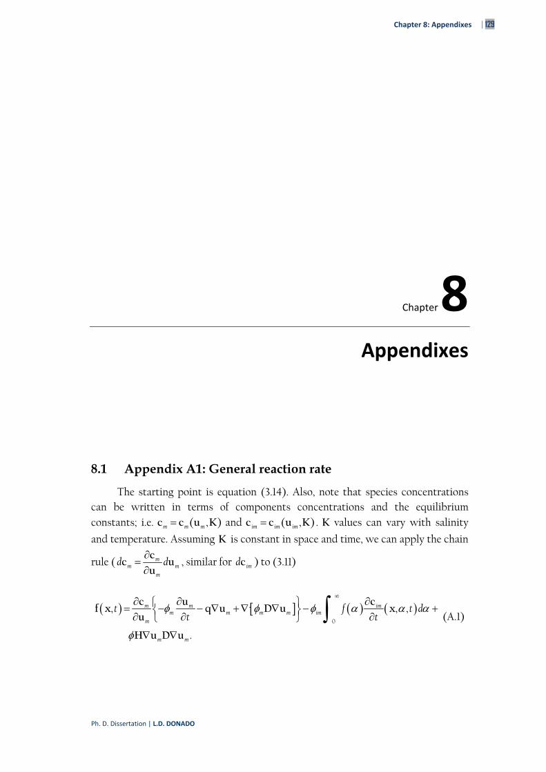
Chapter 8: Appendixes | 129
Ph. D. Dissertation | L.D. DONADO
Chapter 8
Appendixes
8 APPENDIXES
8.1 Appendix A1: General reaction rate
The starting point is equation (3.14). Also, note that species concentrations can be written in terms of components concentrations and the equilibrium constants; i.e. ( , )m m mc c u K and ( , )im im imc c u K . K values can vary with salinity
and temperature. Assuming K is constant in space and time, we can apply the chain
rule ( mm m
m
d d
cc u
u, similar for imdc ) to (3.11)
0
, · , ,
.
m m imm m m m im
m
m m
t f t dt t
c u cf x q u D u x
u
H u D u
(A.1)
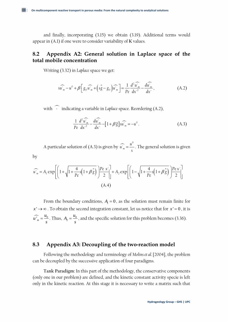
130 | On multicomponent reactive transport in porous media: From the natural complexity to analytical solutions
Hydrogeology Group – GHS | UPC
and finally, incorporating (3.15) we obtain (3.19). Additional terms would appear in (A.1) if one were to consider variability of K values.
8.2 Appendix A2: General solution in Laplace space of the total mobile concentration
Writing (3.32) in Laplace space we get:
2
00 0 2
1 ' '' ' '
' 'm m
m m m
d u dusu u g u s g g u
Pe dx dx , (A.2)
with indicating a variable in Laplace space. Reordering (A.2),
2
02
1 ' '1 '
' 'm m
m
d u dug su u
Pe dx dx . (A.3)
A particular solution of (A.3) is given by 0
'm
uu
s . The general solution is given
by
1 2
4 ' 4 '' exp 1 1 1 exp 1 1 1
2 2m
Pe x Pe xu A s g A s g
Pe Pe
(A.4)
From the boundary conditions, 1 0A , as the solution must remain finite for
'x . To obtain the second integration constant, let us notice that for ' 0x , it is
0'mu
us
. Thus, 02
uA
s , and the specific solution for this problem becomes (3.36).
8.3 Appendix A3: Decoupling of the two-reaction model
Following the methodology and terminology of Molins et al. [2004], the problem can be decoupled by the successive application of four paradigms.
Tank Paradigm: In this part of the methodology, the conservative components (only one in our problem) are defined, and the kinetic constant activity specie is left only in the kinetic reaction. At this stage it is necessary to write a matrix such that
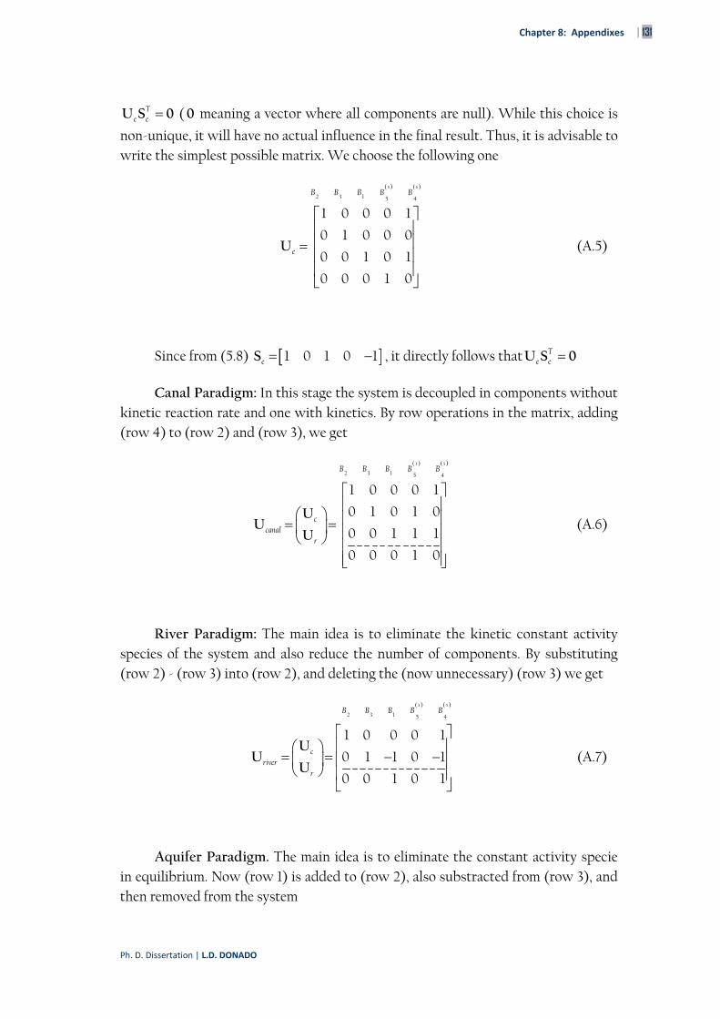
Chapter 8: Appendixes | 131
Ph. D. Dissertation | L.D. DONADO
Te eU S 0 ( 0 meaning a vector where all components are null). While this choice is
non-unique, it will have no actual influence in the final result. Thus, it is advisable to write the simplest possible matrix. We choose the following one
( ) ( )
2 3 1 5 4
1 0 0 0 1
0 1 0 0 0
0 0 1 0 1
0 0 0 1 0
s s
e
B B B B B
U (A.5)
Since from (5.8) 1 0 1 0 1eS , it directly follows that Te eU S 0
Canal Paradigm: In this stage the system is decoupled in components without kinetic reaction rate and one with kinetics. By row operations in the matrix, adding (row 4) to (row 2) and (row 3), we get
( ) ( )
2 3 1 5 4
1 0 0 0 1
0 1 0 1 0
0 0 1 1 1
0 0 0 1 0
s s
ccanal
r
B B B B B
UU
U (A.6)
River Paradigm: The main idea is to eliminate the kinetic constant activity species of the system and also reduce the number of components. By substituting (row 2) - (row 3) into (row 2), and deleting the (now unnecessary) (row 3) we get
( ) ( )
2 3 1 5 4
1 0 0 0 1
0 1 1 0 1
0 0 1 0 1
s s
criver
r
B B B B B
UU
U (A.7)
Aquifer Paradigm. The main idea is to eliminate the constant activity specie in equilibrium. Now (row 1) is added to (row 2), also substracted from (row 3), and then removed from the system
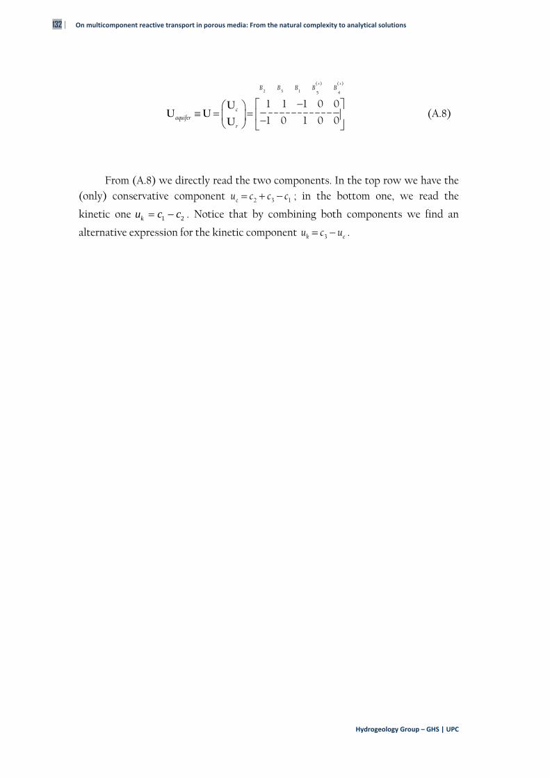
132 | On multicomponent reactive transport in porous media: From the natural complexity to analytical solutions
Hydrogeology Group – GHS | UPC
( ) ( )
2 3 1 5 4
1 1 1 0 0
1 0 1 0 0
s s
caquifer
r
B B B B B
UU U
U (A.8)
From (A.8) we directly read the two components. In the top row we have the (only) conservative component 2 3 1eu c c c ; in the bottom one, we read the
kinetic one 1 2ku c c . Notice that by combining both components we find an
alternative expression for the kinetic component 3k eu c u .

(This page intentionally left blank.)

© 2003 – 2009


